Embed Size (px)
Citation preview
15Eng Sanit Ambient | v.23 n.1 | jan/fev 2018 | 15-25
ABSTRACTThe characterization of sediment input in watersheds is an important
tool for projects that support soil conservation and watershed
management. A spatial and temporal analysis of the sediment
input in an agricultural watershed tributary of Santa Rita River was
performed by means of a geoprocessing simulation in the municipality
of Fernandópolis, São Paulo, Brazil. In order to accomplish this, there
was a simulation of sediment delivery using the Modified Universal
Soil Loss Equation (MUSLE) method for basins, from October
2012 to September 2013. There was a total of 433.87 t of sediments
contributed in the period evaluated, resulting in an average soil loss of
3,635 t.ha-1.yr-1. The period with the greatest amount of sediment input
was from December 2012 to March 2013. 65.1% of all the sediments were
produced at that time. In the most critical month of sediment input,
February 2013, about 15% of the total basin area showed sediment
contributions ranging from 2 to 15 t.ha-1.yr-1. Sugarcane contributed the
most sediment, accounting for 92% of the total, and an average of 6,343
t.ha-1.yr-1.
Keywords: slope; diffuse pollution; water resources; land use and
occupation.
1Specialization in High School Teaching; Technician and Higher Up in Occupational Safety Engineering and in Environmental Quality Management and Control; Technician in Sugar and Alcohol. Microlins Professor at the Fundação Educacional de Fernandópolis and at the Escola Técnica Estadual de Fernandópolis – Fernandópolis (SP), Brazil.2PhD in Agronomy from the Universidade Estadual Paulista “Júlio de Mesquita Filho”. Full Professor in the undergraduate department of Agronomy at the Universidade Camilo Castelo Branco and in the undergraduate department of Environmental and Sanitary Engineering at the Fundação Educacional de Fernandópolis. Coordinator of the Post-graduate Stricto Sensu Program in in Environmental Sciences at the Universidade Camilo Castelo Branco – Fernandópolis (SP), Brazil. Mailing address: Luiz Sergio Vanzela – Avenida Rosalvo Aderaldo, 1729 – Santo Afonso – 15600-000 – Fernandópolis (SP), Brazil – E-mail: [email protected] Received on: 08/25/16 – Accepted on: 12/01/16 – Reg. ABES: 154987
Technical Note
A temporal and spatial simulation of the sediment input in an agricultural basin in the
municipality of Fernandópolis, São Paulo, BrazilSimulação temporal e espacial do aporte de sedimentos em bacia agrícola no município de Fernandópolis (SP)
Elaine Cristina Siqueira1, Luiz Sergio Vanzela2
RESUMOA caracterização do aporte de sedimentos em bacias hidrográficas representa
uma importante ferramenta para subsidiar projetos de conservação do solo
e de manejo de bacias hidrográficas. Assim, neste trabalho realizou-se uma
análise temporal e espacial do aporte de sedimentos em bacia hidrográfica
agrícola afluente do Ribeirão Santa Rita, situada em Fernandópolis, São Paulo,
por meio de simulação com o uso de geoprocessamento. Para isto, realizou-
se a simulação do aporte de sedimentos pelo método da equação universal
de perda de solo modificada para bacias, no período de outubro de 2012 a
setembro de 2013. Verificou-se um aporte total de sedimentos de 433,87 t
no período avaliado, resultando em uma perda média de solo de 3,635 t.ha-1.
ano-1. O período de maior aporte de sedimentos foi de dezembro de 2012 a
março de 2013, quando foram produzidos 65,1% do total de sedimentos do
período avaliado. No mês mais crítico, fevereiro de 2013, cerca de 15% da área
total da bacia apresentou aportes de sedimentos variando de 2 a 15 t.ha-1.ano-1.
A cultura da cana-de-açúcar foi a que mais contribuiu com os aportes de
sedimentos, sendo responsável por 92% do total e com média de 6,343 t.ha-1.ano-1.
Palavras-chave: declividade; poluição difusa; recursos hídricos; uso e
ocupação do solo.
INTRODUCTION
The agricultural occupation of watersheds in the last few decades have caused numerous problems related to the degradation of riparian forests and the precarious conservation of the soil. Consequences of the occupa-tion include the reduction in the availability of water in addition to water quality problems (TUNDISI and TUNDISI, 2010). Among the main fac-tors that cause water degradation is the excessive production of sediment,
which is associated with the processes of displacement, transport, depo-sition and compaction. These processes obey the natural laws of terrain (CARVALHO, 2008, p.73), which are usually strengthened in places with constant modifications in land use and occupation (SCAPIN, 2005).
Vegetative soil covers allows the kinetic energy from rain dropping on surfaces to dissipate, reducing the initial disintegration of the soil particles and, consequently, the sediment concentration in the runoff. Moreover, the soil cover represents a mechanical obstacle to the free
DOI: 10.1590/S1413-41522018154987
16 Eng Sanit Ambient | v.23 n.1 | jan/fev 2018 | 15-25
Siqueira, E.C. & Vanzela, L.S.
surface water runoff, causing a decrease in the velocity and the capacity of disintegration, and the transport of sediments (SILVA et al., 2005). Effects such as these were already verified by Donadio, Galbiatti and Paula (2005), who, evaluating the influence of the remaining natural vegetation and agricultural activities on water quality in four springs, concluded that the sampling periods, as well as the soil characteristics and their different uses, influence the water quality of the sub-basins.
Thus, the rational management of watersheds should allow for the min-imization of the diffuse transport of sediments, since, besides being com-posed of minerals and organic matter, they may have nutrients and defenses, which degrade water quality and the environment (MILLER et al., 2013).
In order to evaluate the impacts of human actions and the proposed solutions (MANGO et al., 2011), the characterization of sediment trans-port in watersheds is of extreme importance for river basin manage-ment plans (OYARZÚN et al., 2011). Among the ways of evaluating the potential of sediments that originated from erosion processes, it is worth highlighting the sediment input, which refers to the total soil loss potential of a watershed (SILVA, SCHULZ; CAMARGO, 2003).
Sediment input can be determined by several methods. The Modified Universal Soil Loss Equation (MUSLE) method stands out. It is estimated
from variables that relate to type, slope, land use and land occupation, as well as surface runoff and flood discharge (CHAVES, PIAU, 2008). Considering that within a watershed these variables are integrated and have great spatial variability, with the use of geoprocessing, it is pos-sible to map the origins of the sediment inputs that are above a toler-able amount, which then allows for the implementation of proposals that mitigate erosive processes.
Thus, the objective of this work was to evaluate the temporal and spatial variability of the sediment input in an agricultural watershed located in the municipality of Fernandópolis, in the Northwest region of São Paulo. It was carried out by means of a simulation and with the use of geoprocessing.
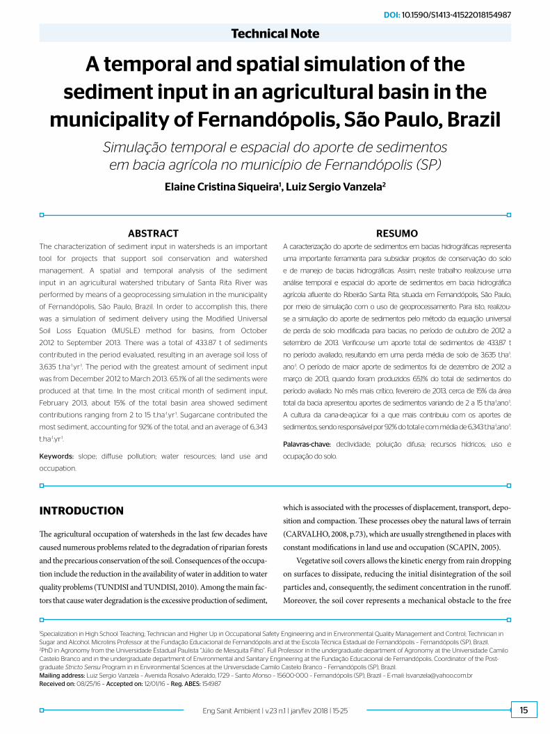
METHODOLOGYThis work was conducted in an agricultural watershed located in the municipality of Fernandópolis, São Paulo. It has a total area of 1,309 km2 and is a tributary of Ribeirão Santa Rita, which is located between the coordinates 20º17’30” and 20º18’15” south, and 50º15’58” and 50º16’51” west (Figure 1).
State of São Paulo
Fernandópolis
Basin 50°15’58”O
20°17’30” S
20°18’15” S
50°16
’51”O
Figure 1 – Map of the location of the basin being studied.
17Eng Sanit Ambient | v.23 n.1 | jan/fev 2018 | 15-25
A simulation of the sediment input in an agricultural basin
MUSCLE was the methodology employed for the simulation of sediment input with the use of geoprocessing, as shown in Equation 1.
( )−
= ⋅ ⋅ ⋅ ⋅ ⋅ ⋅
= ⋅ ⋅− ⋅=+ ⋅
= −
⋅=
= ⋅ ⋅ ⋅
= ⋅+⎝
⎜⎛
⎝⎜⎛
⎝⎜⎛
⎠⎟⎞
⎠⎟⎞
⎠⎟⎞
=⋅
=+
⋅=
⋅=+
=
∑
0,56
3
2
0,5
0,118
0,814
89,6
' 10( 0,2 )'( 0,8 )
25400 254
'
' 0,1667
2 21 1
2π
412
2
1732.921(24,990
)0,0
p
pp
p
e
i i
Y Q q K LS C P
Q Q APP SQP S
SCNq AP
qA
q C i A
CCF C
LFA
CFC A
CA
Titc
LS ⋅ ⋅0,63 1,180984 CV D
(1)
So that,Y is the sediment input in a determined interval of time (t);Q is the volume of surface runoff in a determined interval of time (m3);qp is the maximum flow (m3.s-1);K is the soil erodibility factor (MJ mm ha-1.h-1.year-1);LS is the length factor and degree of slope (dimensionless);C is the management and use factor (dimensionless); andP is the conservationist practices factor (dimensionless).
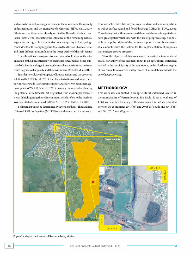
The base material used to obtain all of the coefficients and input variables of the model were the climatic data of the city of Fernandópolis (CIIAGRO, 2014), the software PLÚVIO 2.1 (SILVA
et al., 1999), the soil map (OLIVEIRA et al. al., 1999), the slope map, the watershed map, and the land use and land occupation map (Figure 2).
The sediment input calculations were performed individually for the hydrological units (hu) with an area equivalent to the pixels of a geometric resolution of 2.5 m, that is, with an area of 6.25 m2. These hu are constituted of the combination of type, slope, use and occupa-tion of the land.
Calculating the surface flow volume (step I of the flow chart of Figure 2) was performed by Equation 2.
( )−
= ⋅ ⋅ ⋅ ⋅ ⋅ ⋅
= ⋅ ⋅− ⋅=+ ⋅
= −
⋅=
= ⋅ ⋅ ⋅
= ⋅+⎝
⎜⎛
⎝⎜⎛
⎝⎜⎛
⎠⎟⎞
⎠⎟⎞
⎠⎟⎞
=⋅
=+
⋅=
⋅=+
=
∑
0,56
3
2
0,5
0,118
0,814
89,6
' 10( 0,2 )'( 0,8 )
25400 254
'
' 0,1667
2 21 1
2π
412
2
1732.921(24,990
)0,0
p
pp
p
e
i i
Y Q q K LS C P
Q Q APP SQP S
SCNq AP
qA
q C i A
CCF C
LFA
CFC A
CA
Titc
LS ⋅ ⋅0,63 1,180984 CV D
(2)
So that:Q is the volume of the surface runoff of the pixel (m3);Q’ is the surface runoff (mm); andAP is the area of the pixel (m2).
Y
Q
P
S CN
P5d
UO
qp
Ce
C1 A, L
C2
i
A
KMP
LS
CV
D
C
UO
P
D
Climate Data
Map of land use and occupation
Digital model of the terrain
Soil map
PLÚVIO 2.1
Map of the basin
Map of land use and occupation
Digital model of the terrain
I
II
III
IV
V
VI
Figure 2 – Flowchart of the methodology used to obtain the input data when determining sediment input (Y) in 6 stages (I, II, III, IV, V and VI).
18 Eng Sanit Ambient | v.23 n.1 | jan/fev 2018 | 15-25
Siqueira, E.C. & Vanzela, L.S.
The surface runoff was determined in accordance with the method from Soil Conservation Service (PRUSKI; BRANDÃO; SILVA, 2003), from Equation 3.
( )−
= ⋅ ⋅ ⋅ ⋅ ⋅ ⋅
= ⋅ ⋅− ⋅=+ ⋅
= −
⋅=
= ⋅ ⋅ ⋅
= ⋅+⎝
⎜⎛
⎝⎜⎛
⎝⎜⎛
⎠⎟⎞
⎠⎟⎞
⎠⎟⎞
=⋅
=+
⋅=
⋅=+
=
∑
0,56
3
2
0,5
0,118
0,814
89,6
' 10( 0,2 )'( 0,8 )
25400 254
'
' 0,1667
2 21 1
2π
412
2
1732.921(24,990
)0,0
p
pp
p
e
i i
Y Q q K LS C P
Q Q APP SQP S
SCNq AP
qA
q C i A
CCF C
LFA
CFC A
CA
Titc
LS ⋅ ⋅0,63 1,180984 CV D
(3)
So that:Q’ is the surface runoff (mm);P is the accumulated precipitation in a determined time interval (mm); andS is the maximum capacity for soil storage (mm).
Equation 3 is valid for the situation where P > 0.2S. For the sit-uations where P ≤ 0.2S, the value of Q was equal to 0. The P val-ues were obtained from the data available in the database from the Agrometeorological Information Center of Fernandópolis’ automatic station, which is located 500 m from the studied basin. The value of S was determined by Equation 4.
( )−
= ⋅ ⋅ ⋅ ⋅ ⋅ ⋅
= ⋅ ⋅− ⋅=+ ⋅
= −
⋅=
= ⋅ ⋅ ⋅
= ⋅+⎝
⎜⎛
⎝⎜⎛
⎝⎜⎛
⎠⎟⎞
⎠⎟⎞
⎠⎟⎞
=⋅
=+
⋅=
⋅=+
=
∑
0,56
3
2
0,5
0,118
0,814
89,6
' 10( 0,2 )'( 0,8 )
25400 254
'
' 0,1667
2 21 1
2π
412
2
1732.921(24,990
)0,0
p
pp
p
e
i i
Y Q q K LS C P
Q Q APP SQP S
SCNq AP
qA
q C i A
CCF C
LFA
CFC A
CA
Titc
LS ⋅ ⋅0,63 1,180984 CV D
(4)
So that:S is the maximum capacity of soil storage (mm); andCN is the number of the corrected curves with antecedent soil moisture.
The number of the curve was corrected with the antecedent soil moisture, from the equations:1. CN = 0.0077 CNII
2 + 0.1694CNII + 2.1658 (r² = 0.9978), for the accu-mulated precipitation of the last 5 days (P5d) less than 35.0 mm;
2. CN = CNII, for the accumulated precipitation of the last 5 days (P5d) between 35.0 and 52.5 mm;
3. CN = -0.0067CNII2 + 1.596 CNII + 6.9307 (r² = 0.9000), for
the accumulated precipitation of the last 5 days (P5d) above 52.5 mm.
The values of CNII adopted by the different land use and land occu-pations of the hu are showed in Table 1.
The calculation of maximum flow provided by the hu (stage II of the flow chart of Figure 2) was determined by equation 5.
( )−
= ⋅ ⋅ ⋅ ⋅ ⋅ ⋅
= ⋅ ⋅− ⋅=+ ⋅
= −
⋅=
= ⋅ ⋅ ⋅
= ⋅+⎝
⎜⎛
⎝⎜⎛
⎝⎜⎛
⎠⎟⎞
⎠⎟⎞
⎠⎟⎞
=⋅
=+
⋅=
⋅=+
=
∑
0,56
3
2
0,5
0,118
0,814
89,6
' 10( 0,2 )'( 0,8 )
25400 254
'
' 0,1667
2 21 1
2π
412
2
1732.921(24,990
)0,0
p
pp
p
e
i i
Y Q q K LS C P
Q Q APP SQP S
SCNq AP
qA
q C i A
CCF C
LFA
CFC A
CA
Titc
LS ⋅ ⋅0,63 1,180984 CV D
(5)
So that:qp is the maximum flow of the hu (m3 s-1);qp’ is the maximum flow of the watershed (m3 s-1);AP is the area of the pixel (m2); andA is the drainage area of the basin (m2).
The calculation of the maximum flow of the watershed (qp’) was determined by the rational method (DAEE, 2005), from Equation 6.
( )−
= ⋅ ⋅ ⋅ ⋅ ⋅ ⋅
= ⋅ ⋅− ⋅=+ ⋅
= −
⋅=
= ⋅ ⋅ ⋅
= ⋅+⎝
⎜⎛
⎝⎜⎛
⎝⎜⎛
⎠⎟⎞
⎠⎟⎞
⎠⎟⎞
=⋅
=+
⋅=
⋅=+
=
∑
0,56
3
2
0,5
0,118
0,814
89,6
' 10( 0,2 )'( 0,8 )
25400 254
'
' 0,1667
2 21 1
2π
412
2
1732.921(24,990
)0,0
p
pp
p
e
i i
Y Q q K LS C P
Q Q APP SQP S
SCNq AP
qA
q C i A
CCF C
LFA
CFC A
CA
Titc
LS ⋅ ⋅0,63 1,180984 CV D
(6)
So that:qp is the maximum flow (m3 s-1);C is the surface runoff coefficient;i is the maximum rainfall intensity (mm h-1); andA is the drainage area of the waershed (ha).
The surface runoff coefficient (Ce) of the basin was determined by Equation 7.
( )−
= ⋅ ⋅ ⋅ ⋅ ⋅ ⋅
= ⋅ ⋅− ⋅=+ ⋅
= −
⋅=
= ⋅ ⋅ ⋅
= ⋅+⎝
⎜⎛
⎝⎜⎛
⎝⎜⎛
⎠⎟⎞
⎠⎟⎞
⎠⎟⎞
=⋅
=+
⋅=
⋅=+
=
∑
0,56
3
2
0,5
0,118
0,814
89,6
' 10( 0,2 )'( 0,8 )
25400 254
'
' 0,1667
2 21 1
2π
412
2
1732.921(24,990
)0,0
p
pp
p
e
i i
Y Q q K LS C P
Q Q APP SQP S
SCNq AP
qA
q C i A
CCF C
LFA
CFC A
CA
Titc
LS ⋅ ⋅0,63 1,180984 CV D
(7)
So that:Ce is the surface runoff coefficient of the basin;F is the shape factor of the basin;C1 is the shape coefficient of the basin; eC2 is the volumetric runoff coefficient;
The shape factor (F) was determined by Equation 8.
( )−
= ⋅ ⋅ ⋅ ⋅ ⋅ ⋅
= ⋅ ⋅− ⋅=+ ⋅
= −
⋅=
= ⋅ ⋅ ⋅
= ⋅+⎝
⎜⎛
⎝⎜⎛
⎝⎜⎛
⎠⎟⎞
⎠⎟⎞
⎠⎟⎞
=⋅
=+
⋅=
⋅=+
=
∑
0,56
3
2
0,5
0,118
0,814
89,6
' 10( 0,2 )'( 0,8 )
25400 254
'
' 0,1667
2 21 1
2π
412
2
1732.921(24,990
)0,0
p
pp
p
e
i i
Y Q q K LS C P
Q Q APP SQP S
SCNq AP
qA
q C i A
CCF C
LFA
CFC A
CA
Titc
LS ⋅ ⋅0,63 1,180984 CV D
(8)
So that:F is the shape factor of the basin;A is the drainage area of the watershed (km2); andL is the length of the main talvegue (km).
The shape coefficient (C1) was determined by Equation 9.
( )−
= ⋅ ⋅ ⋅ ⋅ ⋅ ⋅
= ⋅ ⋅− ⋅=+ ⋅
= −
⋅=
= ⋅ ⋅ ⋅
= ⋅+⎝
⎜⎛
⎝⎜⎛
⎝⎜⎛
⎠⎟⎞
⎠⎟⎞
⎠⎟⎞
=⋅
=+
⋅=
⋅=+
=
∑
0,56
3
2
0,5
0,118
0,814
89,6
' 10( 0,2 )'( 0,8 )
25400 254
'
' 0,1667
2 21 1
2π
412
2
1732.921(24,990
)0,0
p
pp
p
e
i i
Y Q q K LS C P
Q Q APP SQP S
SCNq AP
qA
q C i A
CCF C
LFA
CFC A
CA
Titc
LS ⋅ ⋅0,63 1,180984 CV D
(9)
Table 1 – Curve number values (CNII) adopted for the different uses and
occupations in the hydrological units.
Description CNII
Pasture 79
Building area 92
Meadows 79
Woods 52
Perennial crops 76
Sugar cane 76
Paved roads 98
19Eng Sanit Ambient | v.23 n.1 | jan/fev 2018 | 15-25
A simulation of the sediment input in an agricultural basin
The volumetric runoff coefficient (C2) was determined by Equation 10.
( )−
= ⋅ ⋅ ⋅ ⋅ ⋅ ⋅
= ⋅ ⋅− ⋅=+ ⋅
= −
⋅=
= ⋅ ⋅ ⋅
= ⋅+⎝
⎜⎛
⎝⎜⎛
⎝⎜⎛
⎠⎟⎞
⎠⎟⎞
⎠⎟⎞
=⋅
=+
⋅=
⋅=+
=
∑
0,56
3
2
0,5
0,118
0,814
89,6
' 10( 0,2 )'( 0,8 )
25400 254
'
' 0,1667
2 21 1
2π
412
2
1732.921(24,990
)0,0
p
pp
p
e
i i
Y Q q K LS C P
Q Q APP SQP S
SCNq AP
qA
q C i A
CCF C
LFA
CFC A
CA
Titc
LS ⋅ ⋅0,63 1,180984 CV D
(10)
So that:C2 is the volumetric runoff coefficient;Ci is the volumetric runoff coefficient of the use and occupation “i”;Ai is the total area of use and occupation “i” (km2); andA drainage area of the watershed (km2).
The volumetric runoff coefficient (Ci) was assigned for each land use and occupation according to Table 2.
The maximum rain intensity (i) was determined using the equa-tion of intensity, duration, and frequency of rainfall with the aid of the software PLÚVIO 2.1 (SILVA et al., 1999). The equation for the loca-tion of the studied watershed was Equation 11.
Table 2 – Values adopted for the volumetric runoff coefficient (Ci) for
each land use and occupation in the basin.
Description Ci
Pasture 0.25
Building area 0.70
Meadows 0.25
Woods 0.20
Perennial crops 0.30
Sugar cane 0.35
Paved roads 0.70
( )−
= ⋅ ⋅ ⋅ ⋅ ⋅ ⋅
= ⋅ ⋅− ⋅=+ ⋅
= −
⋅=
= ⋅ ⋅ ⋅
= ⋅+⎝
⎜⎛
⎝⎜⎛
⎝⎜⎛
⎠⎟⎞
⎠⎟⎞
⎠⎟⎞
=⋅
=+
⋅=
⋅=+
=
∑
0,56
3
2
0,5
0,118
0,814
89,6
' 10( 0,2 )'( 0,8 )
25400 254
'
' 0,1667
2 21 1
2π
412
2
1732.921(24,990
)0,0
p
pp
p
e
i i
Y Q q K LS C P
Q Q APP SQP S
SCNq AP
qA
q C i A
CCF C
LFA
CFC A
CA
Titc
LS ⋅ ⋅0,63 1,180984 CV D
(11)
So that:i is the maximum rainfall intensity (mm h-1);T is the period of return (years), considered 10 years; andct is the concentration time (min).
The soil erodibility factor (K) (stage III of the flowchart of Figure 2), which was adopted for the entire watershed (considering that these are argisols, according to the pedological map of the state of São Paulo) (OLIVEIRA et al., 1999), was 0.04 MJ mm ha-1.year-1.
The degree factor and slope length (SL) (stage IV of the flow chart from Figure 2) was obtained for the hydrological units, according to Bertoni and Lombardi Neto (1999), using Equation 12.
( )−
= ⋅ ⋅ ⋅ ⋅ ⋅ ⋅
= ⋅ ⋅− ⋅=+ ⋅
= −
⋅=
= ⋅ ⋅ ⋅
= ⋅+⎝
⎜⎛
⎝⎜⎛
⎝⎜⎛
⎠⎟⎞
⎠⎟⎞
⎠⎟⎞
=⋅
=+
⋅=
⋅=+
=
∑
0,56
3
2
0,5
0,118
0,814
89,6
' 10( 0,2 )'( 0,8 )
25400 254
'
' 0,1667
2 21 1
2π
412
2
1732.921(24,990
)0,0
p
pp
p
e
i i
Y Q q K LS C P
Q Q APP SQP S
SCNq AP
qA
q C i A
CCF C
LFA
CFC A
CA
Titc
LS ⋅ ⋅0,63 1,180984 CV D (12)
So that:SL is the factor of the length and degree of the slope (m);FL is the flow path length (m); andD is the declivity (%).
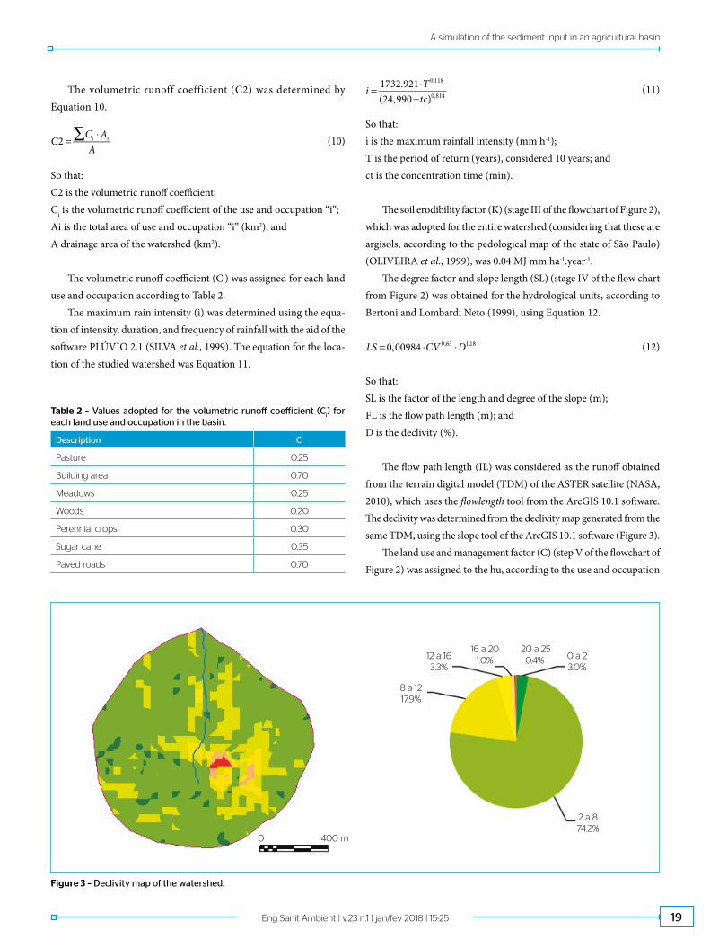
The flow path length (IL) was considered as the runoff obtained from the terrain digital model (TDM) of the ASTER satellite (NASA, 2010), which uses the flowlength tool from the ArcGIS 10.1 software. The declivity was determined from the declivity map generated from the same TDM, using the slope tool of the ArcGIS 10.1 software (Figure 3).
The land use and management factor (C) (step V of the flowchart of Figure 2) was assigned to the hu, according to the use and occupation
2 a 874.2%
0 400 m
12 a 163.3%
16 a 201.0%
20 a 250.4% 0 a 2
3.0%
8 a 1217.9%
Figure 3 – Declivity map of the watershed.
20 Eng Sanit Ambient | v.23 n.1 | jan/fev 2018 | 15-25
Siqueira, E.C. & Vanzela, L.S.
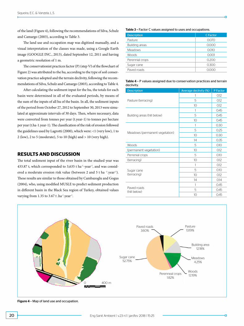
of the land (Figure 4), following the recommendations of Silva, Schulz and Camargo (2003), according to Table 3.
The land use and occupation map was digitized manually, and a visual interpretation of the classes was made, using a Google Earth image (GOOGLE INC., 2013), dated September 12, 2011 and having a geometric resolution of 1 m.
The conservationist practices factor (P) (step VI of the flowchart of Figure 2) was attributed to the hu, according to the type of soil conser-vation practice adopted and the terrain declivity, following the recom-mendations of Silva, Schulz and Camargo (2003), according to Table 4.
After calculating the sediment input for the hu, the totals for each basin were determined in all of the evaluated periods, by means of the sum of the inputs of all hu of the basin. In all, the sediment inputs of the period from October 27, 2012 to September 30, 2013 were simu-lated at approximate intervals of 30 days. Then, where necessary, data were converted from tonnes per year (t.year-1) to tonnes per hectare per year (t.ha-1.year-1). The classification of the risk of erosion followed the guidelines used by Lagrotti (2000), which were: <1 (very low), 1 to 2 (low), 2 to 5 (moderate), 5 to 10 (high) and > 10 (very high).
RESULTS AND DISCUSSIONThe total sediment input of the river basin in the studied year was 433.87 t, which corresponded to 3,635 t ha-1-year-1, and was consid-ered a moderate erosion risk value (between 2 and 5 t ha -1.year-1). These results are similar to those obtained by Cambazoglu and Gogus (2004), who, using modified MUSLE to predict sediment production in different basin in the Black Sea region of Turkey, obtained values varying from 1.35 to 3.67 t .ha-1.year-1.
Table 3 – Factor C values assigned to uses and occupations.
Description C Factor
Pasture 0.070
Building areas 0.000
Meadows 0.010
Woods 0.001
Perennial crops 0.200
Sugar cane 0.300
Paved roads 0.000
Table 4 – P values assigned due to conservation practices and terrain declivity.
Description Average declivity (%) P Factor
Pasture (terracing)
1 0.12
5 0.12
10 0.12
Building areas (hill below)
1 0.45
5 0.45
10 0.45
Meadows (permanent vegetation)
1 0.30
5 0.25
10 0.30
14 0.35
Woods 5 0.10
(permanent vegetation) 10 0.12
Perrenial crops 5 0.10
(terracing) 10 0.12
Sugar cane(terracing)
1 0.12
5 0.10
10 0.12
14 0.14
Paved roads(hill below)
1 0.45
5 0.45
10 0.45
0 400 m
Paved roads3.60%
Sugar cane52.75%
Perenneal crops1.82%
Woods12.19%
Meadows4.25%
Building area12.18%
Pasture13.19%
Figure 4 – Map of land use and occupation.
21Eng Sanit Ambient | v.23 n.1 | jan/fev 2018 | 15-25
A simulation of the sediment input in an agricultural basin
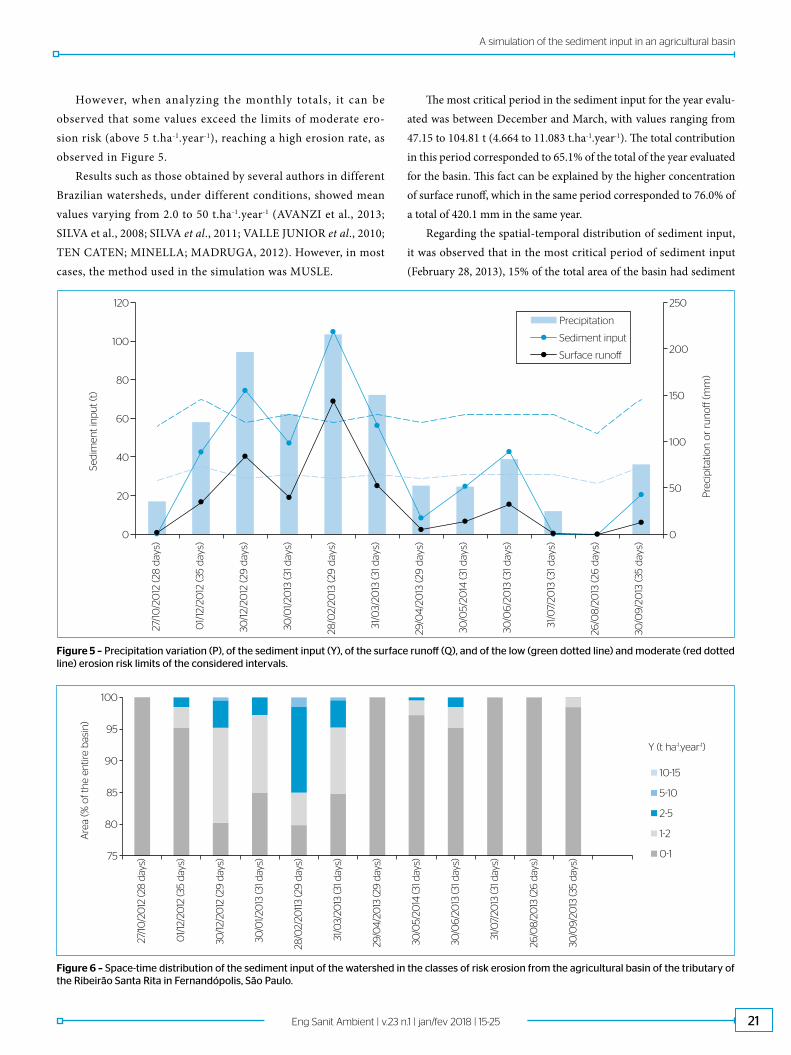
However, when analyzing the monthly totals, it can be observed that some values exceed the limits of moderate ero-sion risk (above 5 t.ha-1.year-1), reaching a high erosion rate, as observed in Figure 5.
Results such as those obtained by several authors in different Brazilian watersheds, under different conditions, showed mean values varying from 2.0 to 50 t.ha-1.year-1 (AVANZI et al., 2013; SILVA et al., 2008; SILVA et al., 2011; VALLE JUNIOR et al., 2010; TEN CATEN; MINELLA; MADRUGA, 2012). However, in most cases, the method used in the simulation was MUSLE.
The most critical period in the sediment input for the year evalu-ated was between December and March, with values ranging from 47.15 to 104.81 t (4.664 to 11.083 t.ha-1.year-1). The total contribution in this period corresponded to 65.1% of the total of the year evaluated for the basin. This fact can be explained by the higher concentration of surface runoff, which in the same period corresponded to 76.0% of a total of 420.1 mm in the same year.
Regarding the spatial-temporal distribution of sediment input, it was observed that in the most critical period of sediment input (February 28, 2013), 15% of the total area of the basin had sediment
0
50
100
150
200
250
0
20
40
60
80
100
120
Pre
cip
itatio
n o
r ru
no
� (m
m)
Sed
imen
t in
pu
t (t
)
Precipitation
Sediment input
Surface runo�
27/1
0/2
012
(28
day
s)
01/
12/2
012
(35
day
s)
30/1
2/20
12 (2
9 d
ays)
30/0
1/20
13 (3
1 day
s)
28/0
2/20
13 (2
9 d
ays)
31/0
3/20
13 (3
1 day
s)
29/0
4/2
013
(29
day
s)
30/0
5/20
14 (3
1 day
s)
30/0
6/2
013
(31 d
ays)
31/0
7/20
13 (3
1 day
s)
26/0
8/2
013
(26
day
s)
30/0
9/2
013
(35
day
s)Figure 5 – Precipitation variation (P), of the sediment input (Y), of the surface runoff (Q), and of the low (green dotted line) and moderate (red dotted line) erosion risk limits of the considered intervals.
75
27/1
0/2
012
(28
days
)
01/
12/2
012
(35
days
)
30/1
2/20
12 (2
9 d
ays)
30/0
1/20
13 (3
1 day
s)
28/0
2/20
113
(29
day
s)
31/0
3/20
13 (3
1 day
s)
29/0
4/20
13 (2
9 d
ays)
30/0
5/20
14 (3
1 day
s)
30/0
6/2
013
(31 d
ays)
31/0
7/20
13 (3
1 day
s)
26/0
8/20
13 (2
6 d
ays)
30/0
9/20
13 (3
5 da
ys)
80
85
90
95
100
Are
a (%
of t
he
entir
e b
asin
)
10-15
5-10
2-5
1-2
0-1
Y (t ha-1.year-1)
Figure 6 – Space-time distribution of the sediment input of the watershed in the classes of risk erosion from the agricultural basin of the tributary of the Ribeirão Santa Rita in Fernandópolis, São Paulo.
22 Eng Sanit Ambient | v.23 n.1 | jan/fev 2018 | 15-25
Siqueira, E.C. & Vanzela, L.S.
inputs varying from 2 to 15 t. ha-1.ano-1 (Figure 6), with 1.52% of the basin showing inputs ranging from high to very high risk of erosion (above 5 t.ha-1.year-1).
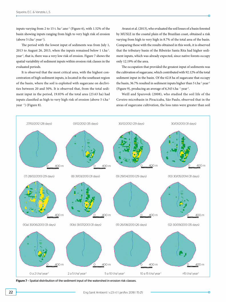
The period with the lowest input of sediments was from July 1, 2013 to August 26, 2013, when the inputs remained below 1 t.ha-1.year-1, that is, there was a very low risk of erosion. Figure 7 shows the spatial variability of sediment inputs within erosion risk classes in the evaluated periods.
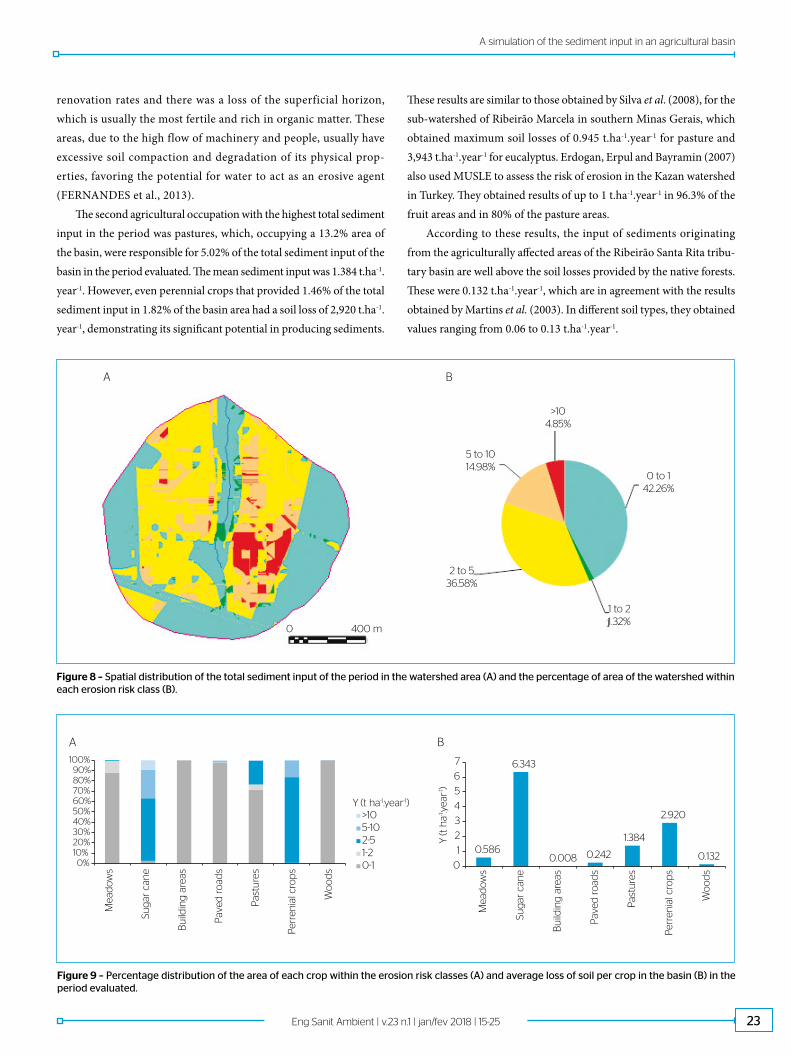
It is observed that the most critical area, with the highest con-centration of high sediment inputs, is located in the southeast region of the basin, where the soil is exploited with sugarcane on declivi-ties between 20 and 50%. It is observed that, from the total sedi-ment input in the period, 19.83% of the total area (23.63 ha) had inputs classified as high to very high risk of erosion (above 5 t.ha-1 year -1) (Figure 8).
>15 t.ha-1.year-1
0 400 m 0 400 m 0 400 m 0 400 m
0 400 m 0 400 m 0 400 m 0 400 m
0 400 m 0 400 m 0 400 m 0 400 m
27/10/2012 (28 days) 01/12/2012 (35 days) 30/12/2012 (29 days) 30/01/2013 (31 days)
(7) 28/02/2013 (29 days) (8) 31/03/2013 (31 days) (9) 29/04/2013 (29 days) (10) 30/05/2014 (31 days)
(10a) 30/06/2013 (31 days) (10b) 31/07/2013 (31 days) (11) 26/08/2013 (26 days) (12) 30/09/2013 (35 days)
0 a 2 t.ha-1.year-1 2 a 5 t.ha-1.year-1 5 a 10 t.ha-1.year-1 10 a 15 t.ha-1.year-1
Figure 7 – Spatial distribution of the sediment input of the watershed in erosion risk classes.
Avanzi et al. (2013), who evaluated the soil losses of a basin forested by MUSLE in the coastal plain of the Brazilian coast, obtained a risk varying from high to very high in 8.7% of the total area of the basin. Comparing these with the results obtained in this work, it is observed that the tributary basin of the Ribeirão Santa Rita had higher sedi-ment inputs, which was already expected, since native forests occupy only 12.19% of the area.
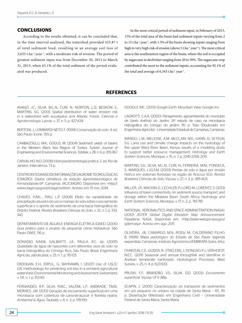
The occupation that provided the greatest input of sediments was the cultivation of sugarcane, which contributed with 92.12% of the total sediment input in the basin. Of the 62.8 ha of sugarcane that occupy the basin, 36.7% resulted in sediment inputs higher than 5 t.ha-1.year-1 (Figure 9), producing an average of 6,343 t.ha -1.year-1.
Weill and Sparovek (2008), who studied the soil life of the Ceveiro microbasin in Piracicaba, São Paulo, observed that in the areas of sugarcane cultivation, the loss rates were greater than soil
23Eng Sanit Ambient | v.23 n.1 | jan/fev 2018 | 15-25
A simulation of the sediment input in an agricultural basin
Figure 9 – Percentage distribution of the area of each crop within the erosion risk classes (A) and average loss of soil per crop in the basin (B) in the period evaluated.
0%10%20%30%40%50%60%70%80%90%
100%
>105-102-51-20-1
Y (t ha-1.year-1)
A B
Mea
do
ws
Sug
ar c
ane
Bu
ildin
g a
reas
Pav
ed r
oad
s
Pas
ture
s
Perr
enia
l cro
ps
Wo
od
s
Mea
do
ws
Sug
ar c
ane
Bu
ildin
g a
reas
Pav
ed r
oad
s
Pas
ture
s
Perr
enia
l cro
ps
Wo
od
s
Y (t
ha-1 .y
ear-1 )
0.586
6.343
0.008 0.242
1.384
2.920
0.1320
1
2
3
4
5
6
7
5 to 1014.98%
A B
0 400 m
2 to 536.58%
1 to 21.32%
0 to 142.26%
>104.85%
Figure 8 – Spatial distribution of the total sediment input of the period in the watershed area (A) and the percentage of area of the watershed within each erosion risk class (B).
renovation rates and there was a loss of the superficial horizon, which is usually the most fertile and rich in organic matter. These areas, due to the high flow of machinery and people, usually have excessive soil compaction and degradation of its physical prop-erties, favoring the potential for water to act as an erosive agent (FERNANDES et al., 2013).
The second agricultural occupation with the highest total sediment input in the period was pastures, which, occupying a 13.2% area of the basin, were responsible for 5.02% of the total sediment input of the basin in the period evaluated. The mean sediment input was 1.384 t.ha-1.year-1. However, even perennial crops that provided 1.46% of the total sediment input in 1.82% of the basin area had a soil loss of 2,920 t.ha-1.year-1, demonstrating its significant potential in producing sediments.
These results are similar to those obtained by Silva et al. (2008), for the sub-watershed of Ribeirão Marcela in southern Minas Gerais, which obtained maximum soil losses of 0.945 t.ha-1.year-1 for pasture and 3,943 t.ha-1.year-1 for eucalyptus. Erdogan, Erpul and Bayramin (2007) also used MUSLE to assess the risk of erosion in the Kazan watershed in Turkey. They obtained results of up to 1 t.ha-1.year-1 in 96.3% of the fruit areas and in 80% of the pasture areas.
According to these results, the input of sediments originating from the agriculturally affected areas of the Ribeirão Santa Rita tribu-tary basin are well above the soil losses provided by the native forests. These were 0.132 t.ha-1.year-1, which are in agreement with the results obtained by Martins et al. (2003). In different soil types, they obtained values ranging from 0.06 to 0.13 t.ha-1.year-1.
24 Eng Sanit Ambient | v.23 n.1 | jan/fev 2018 | 15-25
Siqueira, E.C. & Vanzela, L.S.
CONCLUSIONSAccording to the results obtained, it can be concluded that,
in the time interval analyzed, the watershed provided 433.87 t of total sediment load, resulting in an average soil loss of 3,635 t.ha-1.year-1, with a moderate risk of erosion. The period of greatest sediment input was from December 30, 2012 to March 31, 2013, when 65.1% of the total sediment of the period evalu-ated was produced.
In the most critical period of sediment input, in February of 2013, 15% of the total area of the basin had sediment inputs varying from 2 to 15 t.ha-1.year-1, with 1.5% of the basin showing inputs ranging from high to very high risk of erosion (above 5 t.ha-1.year-1). The most critical area is the southeastern region of the basin, where the soil is occupied by sugarcane in declivities ranging from 20 to 50%. The sugarcane crop contributed the most to the sediment inputs, accounting for 92.1% of the total and average of 6,343 t.ha-1.year-1.
AVANZI, J.C.; SILVA, M.L.N.; CURI, N.; NORTON, L.D.; BESKOW, S.; MARTINS, S.G. (2013) Spatial distribution of water erosion risk in a watershed with eucalyptus and Atlantic Forest. Ciências e Agrotecnologia, Lavras, v. 37, n. 5, p. 427-434.
BERTONI, J.; LOMBARDI NETO, F. (1999) Conservação do solo. 4. ed. São Paulo: Ícone. 355 p.
CAMBAZOGLU, M.K.; GOGUS, M. (2004) Sediment yields of basins in the Western Black Sea Region of Turkey. Turkish Journal of Engineering and Environmental Sciences, Tübitak, v. 28, n. 6, p. 355-367.
CARVALHO, N.O. (2008) Hidrossedimentologia prática. 2. ed. Rio de Janeiro: Interciência. 73 p.
CENTRO INTEGRADO DE INFORMAÇÕES AGROMETEOROLÓGICAS (CIIAGRO). Dados climáticos da estação agrometeorológica de Fernandópolis-SP. Campinas: IAC/CIIAGRO. Disponível em: <http://www.ciiagro.sp.gov.br/ciiagroonline>. Acesso em: 15 nov. 2014.
CHAVES, H.M.L.; PIAU, L.P. (2008) Efeito da variabilidade da precipitação pluvial e do uso e manejo do solo sobre o escoamento superficial e o aporte de sedimento de uma bacia hidrográfica do Distrito Federal. Revista Brasileira Ciências do Solo, v. 32, n. 1, p. 333-343.
DEPARTAMENTO DE ÁGUAS E ENERGIA ELÉTRICA (DAEE). (2005) Guia prático para o projeto de pequenas obras hidráulicas. São Paulo: DAEE. 116 p.
DONADIO, N.M.M.; GALBIATTI, J.A.; PAULA, R.C. de. (2005) Qualidade da água de nascentes com diferentes usos do solo na bacia hidrográfica do Córrego Rico, São Paulo, Brasil. Engenharia Agrícola, Jaboticabal, v. 25, n. 1, p. 115-125.
ERDOGAN, E.H.; ERPUL, G.; BAYRAMIN, İ. (2007) Use of USLE/GIS methodology for predicting soil loss in a semiarid agricultural watershed. Environmental Monitoring and Assessment, Switzerland, v. 131, n. 1, p. 153-161.
FERNANDES, R.P.; SILVA, R.W.C.; SALEMI, L.F.; ANDRADE, T.M.B.; MORAES, J.M. (2013) Geração de escoamento superficial em uma microbacia com cobertura de cana-de-açúcar e floresta ripária. Ambiental & Água, Taubaté, v. 8, n. 3, p. 178-190.
GOOGLE INC. (2013) Google Earth. Mountain View: Google Inc.
LAGROTTI, C.A.A. (2000) Planejamento agroambiental do município de Santo Antônio do Jardim, SP: estudo de caso na microbacia hidrográfica do córrego do jardim. 115 p. Tese (Doutorado em Engenharia Agrícola) – Universidade Estadual de Campinas, Campinas.
MANGO, L.M.; MELESSE, A.M.; McCLAIN, M.E.; GANN, D.; SETEGN, S.G. Land use and climate change impacts on the hydrology of the upper Mara River Basin, Kenya: results of a modeling study to support better resource management. Hidrology and Earth System Sciences, Munique, v. 15, n. 7, p. 2245-2258, 2011.
MARTINS, S.G.; SILVA, M.L.N.; CURI, N.; FERREIRA, M.M.; FONSECA, S.; MARQUES, J.J.G.S.M. (2003) Perdas de solo e água por erosão hídrica em sistemas florestais na região de Aracruz (ES). Revista Brasileira Ciências do Solo, Viçosa, v. 27, n. 3, p. 395-403.
MILLER, J.R.; MACKIN, G.; LECHLER, P.; LORD, M.; LORENTZ, S. (2013) Influence of basin connectivity on sediment source, transport, and storage within the Mkabela Basin, South Africa. Hydrology and Earth System Sciences, Munique, v. 17, n. 2, p. 761-781.
NATIONAL AERONAUTICS AND SPACE ADMINISTRATION (NASA). (2010) ASTER Global Digital Elevation Map Announcement. Pasadena: NASA. Disponível em: <http://asterweb.jpl.nasa.gov/gdem.asp>. Acesso em: ago. 2011.
OLIVEIRA, J.B.; CAMARGO, M.N.; ROSSI, M.; CALDERANO FILHO, B. (1999) Mapa pedológico do Estado de São Paulo: legenda expandida. Campinas: Instituto Agronômico/EMBRAPA Solos. 64 p.
OYARZÚN, C.E.; GODOY, R.; STAELENS, J.; DONOSO, P.J.; VERHOEST, N.E.C. (2011) Seasonal and annual throughfall and stemflow in Andean temperate rainforests. Hydrological Processes, West Sussex, v. 25, n. 4, p. 623-633.
PRUSKI, F.F.; BRANDÃO, V.S.; SILVA, D.D. (2003) Escoamento superficial. Viçosa: UFV. 88p.
SCAPIN, J. (2005) Caracterização do transporte de sedimentos em um pequeno rio urbano na cidade de Santa Maria – RS. 115 p. Dissertação (Mestrado em Engenharia Civil) – Universidade Federal de Santa Maria, Santa Maria.
REFERENCES
25Eng Sanit Ambient | v.23 n.1 | jan/fev 2018 | 15-25
A simulation of the sediment input in an agricultural basin
SILVA, A.M.; MELLO, C.R.; CURI, N.; OLIVEIRA, P.M. (2008) Simulação da variabilidade espacial da erosão hídrica em uma sub-bacia hidrográfica de Latossolos no Sul de Minas Gerais. Revista Brasileira Ciências do Solo, Viçosa, v. 32, n. 5, p. 2125-2134.
SILVA, A.M.; SCHULZ, H.E.; CAMARGO, P.B. (2003) Erosão e hidrossedimentologia em bacias hidrográficas. São Carlos: Rima. 140 p.
SILVA, D.D.; PRUSKI, F.F.; SCHAEFER, C.E.G.R.; AMORIM, R.S.S.; PAIVA, K.W.N. (2005) Efeito da cobertura nas perdas de solo em um argissolo vermelho-amarelo utilizando simulador de chuva. Engenharia Agrícola, Jaboticabal, v. 25, n. 2, p. 409-419.
SILVA, D.D.; VALVERDE, A.D.L.; PRUSKI, F.F.; GONÇALVES, R.A.B. (1999) Estimativa e espacialização dos parâmetros da equação de intensidade-duração-frequência da precipitação para o Estado de São Paulo. Engenharia na Agricultura, Viçosa, v. 7, n. 2, p. 70-87.
SILVA, V.A.; MOREAU, M.S.; MOREAU, A.M.S.; REGO, N.A.C. (2011) Uso da terra e perda de solo na bacia hidrográfica do Rio Colônia, Bahia. Revista Brasileira de Engenharia Agrícola Ambiental, Campina Grande, v. 15, n. 3, p. 310-315.
TEN CATEN, A.; MINELLA, J.P.G.; MADRUGA, P.R.A. (2012) Desintensificação do uso da terra e sua relação com a erosão do solo. Revista Brasileira de Engenharia Agrícola e Ambiental, Campina Grande, v. 16, n. 9, p. 1006-1014.
TUNDISI, J.D.; TUNDISI, T.M. (2010) Impactos potenciais das alterações do Código Florestal nos Recursos Hídricos. Biota Neotropica, São Paulo, v. 10, n. 4, p. 67-76.
VALLE JUNIOR, R.F.; GALBIATTI, J.A.; MARTINS FILHO, M.V.; PISSARRA, T.C.T. (2010) Potencial de erosão da bacia do Rio Uberaba. Engenharia Agrícola, Jaboticabal, v. 30, n. 5, p. 897-908.
WEILL, M.A.M.; SPAROVEK, G. (2008) Estudo da erosão na microbacia do Ceveiro (Piracicaba, SP): II – Interpretação da tolerância de perda de solo utilizando o método do Índice de Tempo de Vida. Revista Brasileira Ciências do Solo, v. 32, n. 2, p. 815-824.
© 2018 Associação Brasileira de Engenharia Sanitária e Ambiental This is an open access article distributed under the terms of the Creative Commons license.