Embed Size (px)
Citation preview
Domain Decomposition-based contour integration
eigenvalue solvers
Vassilis Kalantzisjoint work with
Yousef Saad
Computer Science and Engineering DepartmentUniversity of Minnesota - Twin Cities, USA
SIAM ALA 2015, 10-30-2015
VK, YS (U of M) DD-CINT techniques 10-30-2015 1 / 31
Acknowledgments
Joint work with Eric Polizzi and James Kestyn (UM Amherst).Special thanks to Minnesota Supercomputing Institute for allowingaccess to its supercomputers.Work supported by NSF and DOE (DE-SC0008877).
VK, YS (U of M) DD-CINT techniques 10-30-2015 2 / 31
Contents
1 Introduction
2 The Domain Decomposition framework
3 Domain Decomposition-based contour integration
4 Implementation in HPC architectures
5 Experiments
6 Discussion
VK, YS (U of M) DD-CINT techniques 10-30-2015 3 / 31
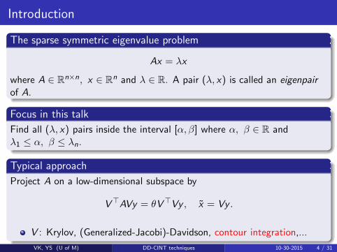
Introduction
The sparse symmetric eigenvalue problem
Ax = λx
where A ∈ Rn×n, x ∈ R
n and λ ∈ R. A pair (λ, x) is called an eigenpair
of A.
Focus in this talk
Find all (λ, x) pairs inside the interval [α, β] where α, β ∈ R andλ1 ≤ α, β ≤ λn.
Typical approach
Project A on a low-dimensional subspace by
V⊤AVy = θV⊤Vy , x̃ = Vy .
V : Krylov, (Generalized-Jacobi)-Davidson, contour integration,...
VK, YS (U of M) DD-CINT techniques 10-30-2015 4 / 31
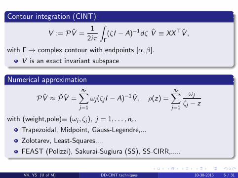
Contour integration (CINT)
V := PV̂ =1
2iπ
∫
Γ(ζI − A)−1dζ V̂ ≡ XX⊤V̂ ,
with Γ → complex contour with endpoints [α, β].
V is an exact invariant subspace
Numerical approximation
PV̂ ≈ P̃V̂ =
nc∑
j=1
ωj(ζj I − A)−1V̂ , ρ(z) =
nc∑
j=1
ωj
ζj − z
with (weight,pole)≡ (ωj , ζj), j = 1, . . . , nc .
Trapezoidal, Midpoint, Gauss-Legendre,...
Zolotarev, Least-Squares,...
FEAST (Polizzi), Sakurai-Sugiura (SS), SS-CIRR,.....
VK, YS (U of M) DD-CINT techniques 10-30-2015 5 / 31
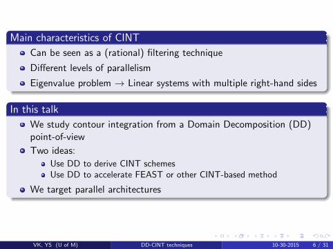
Main characteristics of CINT
Can be seen as a (rational) filtering technique
Different levels of parallelism
Eigenvalue problem → Linear systems with multiple right-hand sides
In this talk
We study contour integration from a Domain Decomposition (DD)point-of-view
Two ideas:
Use DD to derive CINT schemesUse DD to accelerate FEAST or other CINT-based method
We target parallel architectures
VK, YS (U of M) DD-CINT techniques 10-30-2015 6 / 31
Contents
1 Introduction
2 The Domain Decomposition framework
3 Domain Decomposition-based contour integration
4 Implementation in HPC architectures
5 Experiments
6 Discussion
VK, YS (U of M) DD-CINT techniques 10-30-2015 7 / 31
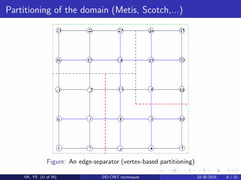
Partitioning of the domain (Metis, Scotch,...)
Figure: An edge-separator (vertex-based partitioning)
VK, YS (U of M) DD-CINT techniques 10-30-2015 8 / 31
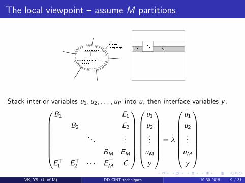
The local viewpoint – assume M partitions
Stack interior variables u1, u2, . . . , uP into u, then interface variables y ,
B1 E1
B2 E2
. . ....
BM EM
E⊤1 E⊤
2 · · · E⊤
M C
u1
u2
...
uM
y
= λ
u1
u2
...
uM
y
VK, YS (U of M) DD-CINT techniques 10-30-2015 9 / 31
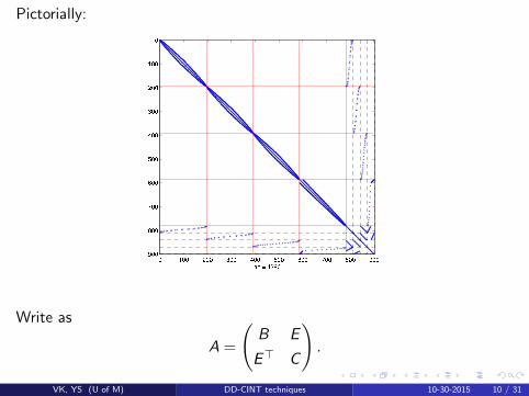
Pictorially:
Write as
A =
(
B E
E⊤ C
)
.
VK, YS (U of M) DD-CINT techniques 10-30-2015 10 / 31
Contents
1 Introduction
2 The Domain Decomposition framework
3 Domain Decomposition-based contour integration
4 Implementation in HPC architectures
5 Experiments
6 Discussion
VK, YS (U of M) DD-CINT techniques 10-30-2015 11 / 31
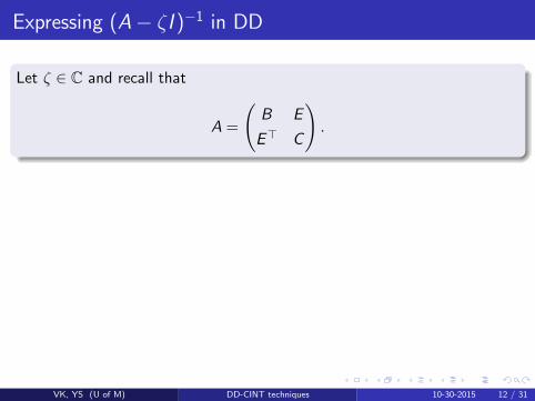
Expressing (A− ζI )−1 in DD
Let ζ ∈ C and recall that
A =
(
B E
E⊤ C
)
.
VK, YS (U of M) DD-CINT techniques 10-30-2015 12 / 31

Expressing (A− ζI )−1 in DD
Let ζ ∈ C and recall that
A =
(
B E
E⊤ C
)
.
Then
(A− ζI )−1 =
(
(B − ζI )−1 + F (ζ)S(ζ)−1F (ζ)⊤ −F (ζ)S(ζ)−1
−S(ζ)−1F (ζ)⊤ S(ζ)−1
)
,
where
F (ζ) = (B − ζI )−1E
S(ζ) = C − ζI − ET (B − ζI )−1E .
VK, YS (U of M) DD-CINT techniques 10-30-2015 12 / 31
Spectral projectors and DD
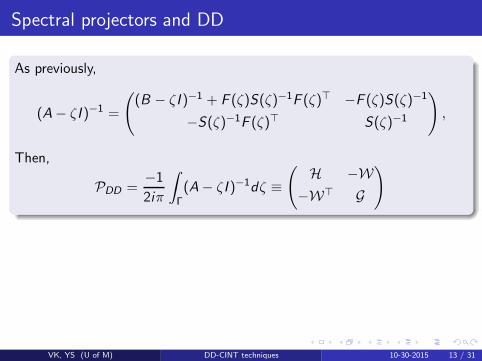
As previously,
(A− ζI )−1 =
(
(B − ζI )−1 + F (ζ)S(ζ)−1F (ζ)⊤ −F (ζ)S(ζ)−1
−S(ζ)−1F (ζ)⊤ S(ζ)−1
)
,
Then,
PDD =−1
2iπ
∫
Γ(A− ζI )−1dζ ≡
(
H −W
−W⊤ G
)
VK, YS (U of M) DD-CINT techniques 10-30-2015 13 / 31
Spectral projectors and DD
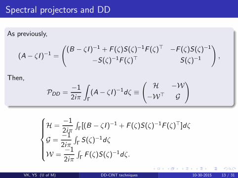
As previously,
(A− ζI )−1 =
(
(B − ζI )−1 + F (ζ)S(ζ)−1F (ζ)⊤ −F (ζ)S(ζ)−1
−S(ζ)−1F (ζ)⊤ S(ζ)−1
)
,
Then,
PDD =−1
2iπ
∫
Γ(A− ζI )−1dζ ≡
(
H −W
−W⊤ G
)
H =−1
2iπ
∫
Γ[(B − ζI )−1 + F (ζ)S(ζ)−1F (ζ)⊤]dζ
G =−1
2iπ
∫
Γ S(ζ)−1dζ
W =−1
2iπ
∫
Γ F (ζ)S(ζ)−1dζ.
VK, YS (U of M) DD-CINT techniques 10-30-2015 13 / 31
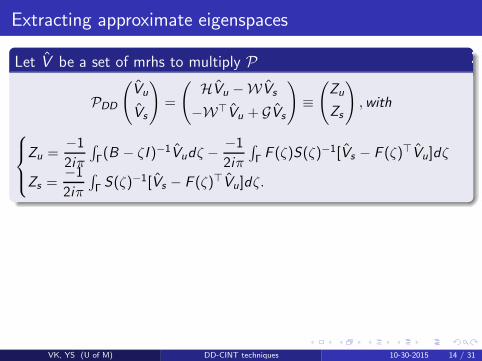
Extracting approximate eigenspaces
Let V̂ be a set of mrhs to multiply P
PDD
(
V̂u
V̂s
)
=
(
HV̂u −WV̂s
−W⊤V̂u + GV̂s
)
≡
(
Zu
Zs
)
,with
Zu =−1
2iπ
∫
Γ(B − ζI )−1V̂udζ −−1
2iπ
∫
Γ F (ζ)S(ζ)−1[V̂s − F (ζ)⊤V̂u]dζ
Zs =−1
2iπ
∫
Γ S(ζ)−1[V̂s − F (ζ)⊤V̂u]dζ.
VK, YS (U of M) DD-CINT techniques 10-30-2015 14 / 31
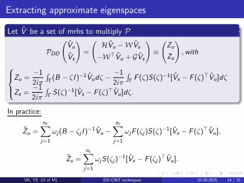
Extracting approximate eigenspaces
Let V̂ be a set of mrhs to multiply P
PDD
(
V̂u
V̂s
)
=
(
HV̂u −WV̂s
−W⊤V̂u + GV̂s
)
≡
(
Zu
Zs
)
,with
Zu =−1
2iπ
∫
Γ(B − ζI )−1V̂udζ −−1
2iπ
∫
Γ F (ζ)S(ζ)−1[V̂s − F (ζ)⊤V̂u]dζ
Zs =−1
2iπ
∫
Γ S(ζ)−1[V̂s − F (ζ)⊤V̂u]dζ.
In practice:
Z̃u =
nc∑
j=1
ωj(B − ζj I )−1V̂u −
nc∑
j=1
ωjF (ζj)S(ζ)−1[V̂s − F (ζ)⊤V̂u],
Z̃s =
nc∑
j=1
ωjS(ζj)−1[V̂s − F (ζj)
⊤V̂u].
VK, YS (U of M) DD-CINT techniques 10-30-2015 14 / 31
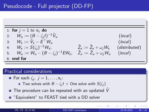
Pseudocode - Full projector (DD-FP)
1: for j = 1 to nc do
2: Wu := (B − ζj I )−1V̂u (local)
3: Ws := V̂s − E⊤Wu (local)4: Ws := S(ζj)
−1Ws ; Z̃s := Z̃s + ωjWs (distributed)5: Wu := Wu − (B − ζj)
−1EWs ; Z̃u := Z̃u + ωjWu (local)6: end for
Practical considerations
For each ζj , j = 1, . . . , nc :
Two solves with B − ζj I + One solve with S(ζj )
The procedure can be repeated with an updated V̂
”Equivalent” to FEAST tied with a DD solver
VK, YS (U of M) DD-CINT techniques 10-30-2015 15 / 31
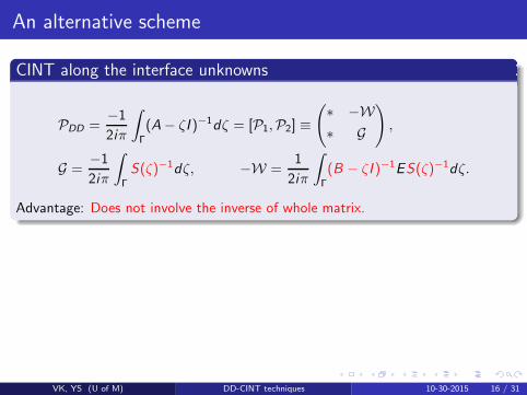
An alternative scheme
CINT along the interface unknowns
PDD =−1
2iπ
∫
Γ
(A− ζI )−1dζ = [P1,P2] ≡
(
∗ −W
∗ G
)
,
G =−1
2iπ
∫
Γ
S(ζ)−1dζ, −W =1
2iπ
∫
Γ
(B − ζI )−1ES(ζ)−1dζ.
Advantage: Does not involve the inverse of whole matrix.
VK, YS (U of M) DD-CINT techniques 10-30-2015 16 / 31
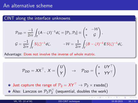
An alternative scheme
CINT along the interface unknowns
PDD =−1
2iπ
∫
Γ
(A− ζI )−1dζ = [P1,P2] ≡
(
∗ −W
∗ G
)
,
G =−1
2iπ
∫
Γ
S(ζ)−1dζ, −W =1
2iπ
∫
Γ
(B − ζI )−1ES(ζ)−1dζ.
Advantage: Does not involve the inverse of whole matrix.
PDD = XX⊤, X =
(
U
Y
)
→ PDD =
(
∗ UY⊤
∗ YY⊤
)
Just capture the range of P2 = XY⊤ → P2 × randn()
Also: Lanczos on P2P⊤2 (sequential, doubles the work)
VK, YS (U of M) DD-CINT techniques 10-30-2015 16 / 31
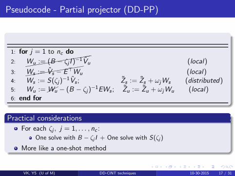
Pseudocode - Partial projector (DD-PP)
1: for j = 1 to nc do
2:✭✭✭✭✭✭✭✭✭✭✭
Wu := (B − ζj I )−1V̂u (local)
3:✭✭✭✭✭✭✭✭✭
Ws := V̂s − E⊤Wu (local)4: Ws := S(ζj)
−1V̂s ; Z̃s := Z̃s + ωjWs (distributed)5: Wu :=✟
✟Wu − (B − ζj)−1EWs ; Z̃u := Z̃u + ωjWu (local)
6: end for
Practical considerations
For each ζj , j = 1, . . . , nc :
One solve with B − ζj I + One solve with S(ζj)
More like a one-shot method
VK, YS (U of M) DD-CINT techniques 10-30-2015 17 / 31
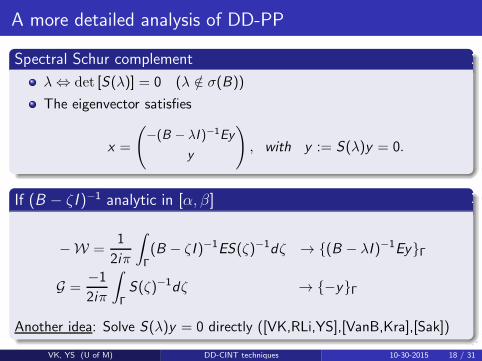
A more detailed analysis of DD-PP
Spectral Schur complement
λ ⇔ det [S(λ)] = 0 (λ /∈ σ(B))
The eigenvector satisfies
x =
(
−(B − λI )−1Ey
y
)
, with y := S(λ)y = 0.
If (B − ζ I )−1 analytic in [α, β]
−W =1
2iπ
∫
Γ(B − ζI )−1ES(ζ)−1dζ → {(B − λI )−1Ey}Γ
G =−1
2iπ
∫
ΓS(ζ)−1dζ → {−y}Γ
Another idea: Solve S(λ)y = 0 directly ([VK,RLi,YS],[VanB,Kra],[Sak])
VK, YS (U of M) DD-CINT techniques 10-30-2015 18 / 31
Contents
1 Introduction
2 The Domain Decomposition framework
3 Domain Decomposition-based contour integration
4 Implementation in HPC architectures
5 Experiments
6 Discussion
VK, YS (U of M) DD-CINT techniques 10-30-2015 19 / 31
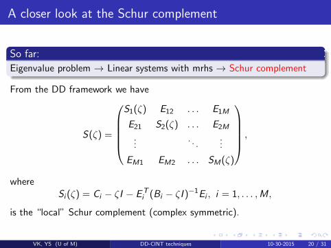
A closer look at the Schur complement
So far:
Eigenvalue problem → Linear systems with mrhs → Schur complement
From the DD framework we have
S(ζ) =
S1(ζ) E12 . . . E1M
E21 S2(ζ) . . . E2M
.... . .
...
EM1 EM2 . . . SM(ζ)
,
whereSi(ζ) = Ci − ζI − ET
i (Bi − ζI )−1Ei , i = 1, . . . ,M,
is the “local” Schur complement (complex symmetric).
VK, YS (U of M) DD-CINT techniques 10-30-2015 20 / 31
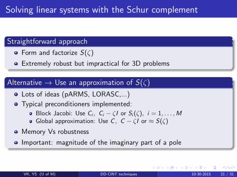
Solving linear systems with the Schur complement
Straightforward approach
Form and factorize S(ζ)
Extremely robust but impractical for 3D problems
Alternative → Use an approximation of S(ζ)
Lots of ideas (pARMS, LORASC,...)
Typical preconditioners implemented:
Block Jacobi: Use Ci , Ci − ζI or Si (ζ), i = 1, . . . ,MGlobal approximation: Use C , C − ζI or ≈ S(ζ)
Memory Vs robustness
Important: magnitude of the imaginary part of a pole
VK, YS (U of M) DD-CINT techniques 10-30-2015 21 / 31
Contents
1 Introduction
2 The Domain Decomposition framework
3 Domain Decomposition-based contour integration
4 Implementation in HPC architectures
5 Experiments
6 Discussion
VK, YS (U of M) DD-CINT techniques 10-30-2015 22 / 31
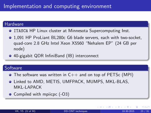
Implementation and computing environment
Hardware
ITASCA HP Linux cluster at Minnesota Supercomputing Inst.
1,091 HP ProLiant BL280c G6 blade servers, each with two-socket,quad-core 2.8 GHz Intel Xeon X5560 “Nehalem EP” (24 GB pernode)
40-gigabit QDR InfiniBand (IB) interconnect
Software
The software was written in C++ and on top of PETSc (MPI)
Linked to AMD, METIS, UMFPACK, MUMPS, MKL-BLAS,MKL-LAPACK
Compiled with mpiicpc (-O3)
VK, YS (U of M) DD-CINT techniques 10-30-2015 23 / 31
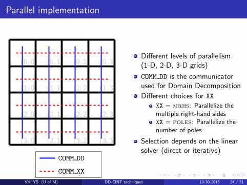
Parallel implementation
(0, 0) (0, 1) (0, 2) (0, 3)
(1, 0) (1, 1) (1, 2) (1, 3)
(2, 0) (2, 1) (2, 2) (2, 3)
(3, 0) (3, 1) (3, 2) (3, 3)
COMM DD
COMM XX
Different levels of parallelism(1-D, 2-D, 3-D grids)
COMM DD is the communicatorused for Domain Decomposition
Different choices for XX
XX = mrhs: Parallelize themultiple right-hand sidesXX = poles: Parallelize thenumber of poles
Selection depends on the linearsolver (direct or iterative)
VK, YS (U of M) DD-CINT techniques 10-30-2015 24 / 31
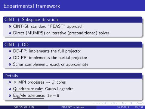
Experimental framework
CINT + Subspace Iteration
CINT-SI: standard ”FEAST” approach
Direct (MUMPS) or iterative (preconditioned) solver
CINT + DD
DD-FP: implements the full projector
DD-PP: implements the partial projector
Schur complement: exact or approximate
Details
# MPI processes → # cores
Quadrature rule: Gauss-Legendre
Eig/vle tolerance: 1e − 8
VK, YS (U of M) DD-CINT techniques 10-30-2015 25 / 31
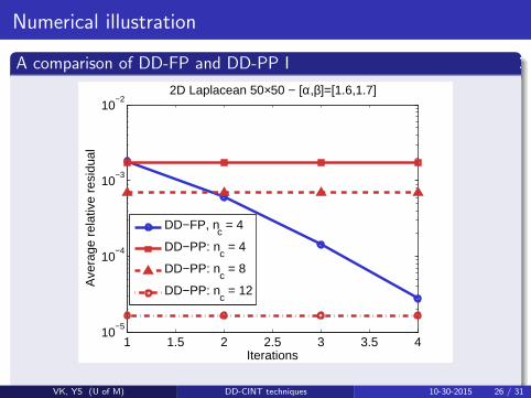
Numerical illustration
A comparison of DD-FP and DD-PP I
1 1.5 2 2.5 3 3.5 410
−5
10−4
10−3
10−2
2D Laplacean 50×50 − [α,β]=[1.6,1.7]
Iterations
Ave
rage
rel
ativ
e re
sidu
al
DD−FP, nc = 4
DD−PP: nc = 4
DD−PP: nc = 8
DD−PP: nc = 12
VK, YS (U of M) DD-CINT techniques 10-30-2015 26 / 31
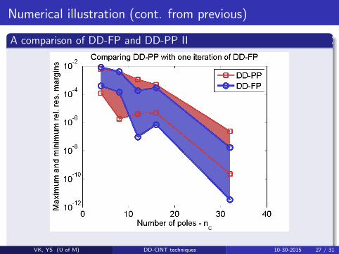
Numerical illustration (cont. from previous)
A comparison of DD-FP and DD-PP II
VK, YS (U of M) DD-CINT techniques 10-30-2015 27 / 31
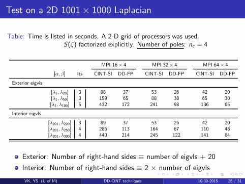
Test on a 2D 1001× 1000 Laplacian
Table: Time is listed in seconds. A 2-D grid of processors was used.S(ζ) factorized explicitly. Number of poles: nc = 4
MPI 16× 4 MPI 32× 4 MPI 64× 4
[α, β] Its CINT-SI DD-FP CINT-SI DD-FP CINT-SI DD-FP
Exterior eigvls
[λ1, λ20] 3 88 37 53 26 42 20[λ1, λ50] 3 159 65 88 38 65 30[λ1, λ100] 5 432 172 241 98 136 65
Interior eigvls
[λ201, λ220] 3 89 37 53 26 42 20[λ201, λ250] 4 286 113 164 67 110 48[λ201, λ300] 4 440 214 245 122 141 84
Exterior: Number of right-hand sides ≡ number of eigvls + 20
Interior: Number of right-hand sides ≡ 2 × number of eigvls
VK, YS (U of M) DD-CINT techniques 10-30-2015 28 / 31
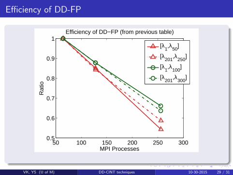
Efficiency of DD-FP
50 100 150 200 250 3000.5
0.6
0.7
0.8
0.9
1R
atio
MPI Processes
Efficiency of DD−FP (from previous table)
[λ1,λ
50]
[λ201
,λ250
]
[λ1,λ
100]
[λ201
,λ300
]
VK, YS (U of M) DD-CINT techniques 10-30-2015 29 / 31
Contents
1 Introduction
2 The Domain Decomposition framework
3 Domain Decomposition-based contour integration
4 Implementation in HPC architectures
5 Experiments
6 Discussion
VK, YS (U of M) DD-CINT techniques 10-30-2015 30 / 31
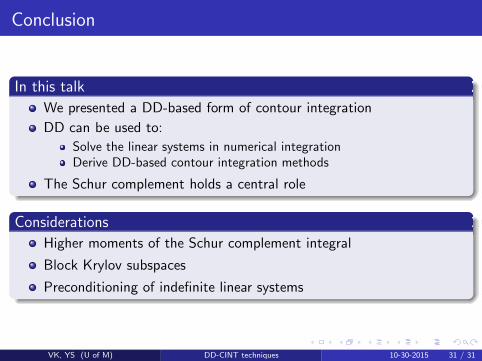
Conclusion
In this talk
We presented a DD-based form of contour integration
DD can be used to:
Solve the linear systems in numerical integrationDerive DD-based contour integration methods
The Schur complement holds a central role
Considerations
Higher moments of the Schur complement integral
Block Krylov subspaces
Preconditioning of indefinite linear systems
VK, YS (U of M) DD-CINT techniques 10-30-2015 31 / 31


![Modified Cholesky Decomposition and Applications McSweeney ... · 2 =nukAk 2 for 100 random matrices of order n= 10 with eigenvalues in [1;10k] and maximum eigenvalue xed as 10k](https://img.pdfslide.net/doc/110x75/5f13e8a24003bc76fb3ba1fe/modiied-cholesky-decomposition-and-applications-mcsweeney-2-nukak-2-for-100.jpg)