DOMINATION AND MATRIX PROPERTIES IN TOURNAMENTS …

DOMINATION AND MATRIX PROPERTIES IN TOURNAMENTS AND

GENERALIZED TOURNAMENTS

by

Dustin J. Stewart

B.S. Mathematics, University of the Pacific, 2001

A thesis submitted to the

University of Colorado at Denver

in partial fulfillment

of the requirements for the degree of

Doctor of Philosophy

Applied Mathematics

2005

This thesis for the Doctor of Philosophy

degree by

Dustin J. Stewart

has been approved

by

J. Richard Lundgren

William E. Cherowitzo

Ellen Gethner

Stanley E. Payne

K. Brooks Reid

Date

Stewart, Dustin J. (Ph.D., Applied Mathematics)

Domination and Matrix Properties in Tournaments and Generalized Tourna-ments

Thesis directed by Professor J. Richard Lundgren

ABSTRACT

In this thesis we examine several matrix properties of tournament matrices.

In particular we look at how domination and related parameters in tournaments

affect these properties in the corresponding matrices. We begin by examin-

ing when a tournament can support an orthogonal matrix. To do so, we first

look at the necessary condition of quadrangularity in tournaments. We classify

tournaments with given properties which meet this necessary condition. We

show how domination effects quadrangularity in regular tournaments and tour-

naments with certain minimum degrees. We also determine for exactly which

orders a quadrangular tournament exists.

In chapter 3, we examine the stronger necessary condition for a digraph to

support an orthogonal matrix of strong quadrangularity. We construct a class

of tournaments which meet this condition. We also show that the 3-cycle is

the unique tournament on ten or fewer vertices which supports an orthogonal

matrix, and discuss a search conducted for a tournament matrix which supports

an orthogonal matrix. In the following chapter we look at which tournament

matrices are fully indecomposable and which are separable, as these properties

iii

are related to a necessary condition for a (0, 1)-matrix to support an orthogonal

matrix. We use our classification to derive a number of matrix and graph theo-

retic corollaries. As the domination graphs of tournaments play a central role in

our classification of separable tournament matrices, we classify the domination

graphs of complete paired comparison digraphs in chapter 5.

Finally, we examine the Boolean, non-negative integer and real ranks of

tournament matrices. We find new bounds for the Boolean rank using results

on dominating sets and related parameters. We determine, for the first time, a

class of tournament matrices in which the real rank is less than the Boolean rank.

We also determine a set theoretic dual to the problem of finding the Boolean row

rank of a tournament matrix, and give some results and conjectures related to

the problem of finding the minimum Boolean rank over all tournament matrices

of order n.

This abstract accurately represents the content of the candidate’s thesis. I

recommend its publication.

SignedJ. Richard Lundgren

iv

DEDICATION

For Melissa, for my family, and for Albion.

ACKNOWLEDGMENT

There are several people in my life that deserve thanks for bringing me to this

point. First, I want to thank my advisor, J. Richard Lundgren. Rich has made

many things possible for me in the last four years, and has taught me a great

deal about mathematics, teaching and life as an academic. I also owe many

thanks my thesis committee Rich, Brooks Reid, Stan Payne, Bill Cherowitzo

and Ellen Gethner. Each have been a great help and influence in their own way.

Thank you as well to the faculty who I had the chance to work with at UCD.

I want to thank the graduate committee and the mathematics department

for the financial support, teaching assistantships and fellowships. None of this

would have been possible without it. Thank you to Marcia Kelly, Liz Lhotka

and Jennifer Thurston. I would not have survived without them. Thanks also

to Lynn Bennethum and Bruce MacMillan for their help and advice on teaching.

My thanks to the UOP mathematics department for preparing me for grad-

uate school, especially to Sarah Merz, Coburn Ward and Vincent Panico. I also

want to thank Sarah for introducing me to graph theory and starting me off

researching in the field.

I am also thankful for my fellow graduate students who have helped me

through the last few years with teaching and research ideas, or by just being

a good distraction. For this, I am happy to thank, among others, Nate, Art,

Ryan, Kevin, Flink, Rob, Tessa, Hank, Sarah and Chris. Special thanks to my

two amazing officemates, Jenny Cowel and Dave Brown, and to Carey Jenkins

and Jeff Matsuo, helpful friends and great fishermen.

I want to thank my parents for everything they have done for me. Especially

for when they sent me to college and started this whole process.

Finally, I want to thank Melissa Cyfers for all her love and support. I could

not have asked for more.

CONTENTS

Figures . . . . . . . . . . . . . . . . . . . . . . . . . . . . . . . . . . . . ix

1. Introduction . . . . . . . . . . . . . . . . . . . . . . . . . . . . . . . . 1

1.1 Background . . . . . . . . . . . . . . . . . . . . . . . . . . . . . . . 1

1.2 Graph and digraph basics . . . . . . . . . . . . . . . . . . . . . . . 4

1.3 Tournament basics . . . . . . . . . . . . . . . . . . . . . . . . . . . 11

1.4 Domination basics . . . . . . . . . . . . . . . . . . . . . . . . . . . 19

1.5 Matrix basics . . . . . . . . . . . . . . . . . . . . . . . . . . . . . . 23

2. Quadrangular Tournaments . . . . . . . . . . . . . . . . . . . . . . . 27

2.1 Definitions and background . . . . . . . . . . . . . . . . . . . . . . 27

2.2 Tournaments which are not strongly connected . . . . . . . . . . . 29

2.3 Tournaments with given minimum degrees . . . . . . . . . . . . . . 34

2.4 Regular and rotational tournaments . . . . . . . . . . . . . . . . . . 38

2.5 Known orders of quadrangular tournaments . . . . . . . . . . . . . 43

3. Strongly Quadrangluar Tournaments . . . . . . . . . . . . . . . . . . 55


3.2 A class of strongly quadrangular tournaments . . . . . . . . . . . . 57

3.3 Nonexistence and searches . . . . . . . . . . . . . . . . . . . . . . . 62

4. Fully Indecomposable Tournament Matrices . . . . . . . . . . . . . . 69


4.2 Fully indecomposable matrices . . . . . . . . . . . . . . . . . . . . . 72

vii

4.3 Separable matrices . . . . . . . . . . . . . . . . . . . . . . . . . . . 74

4.4 Corollaries . . . . . . . . . . . . . . . . . . . . . . . . . . . . . . . . 77

5. Domination Graphs of Complete Paired Comparison Digraphs . . . . 84


5.2 Preliminary results . . . . . . . . . . . . . . . . . . . . . . . . . . . 85

5.3 Complete paired comparison digraphs with no arc weight .5 . . . . 90

5.4 Connected domination graphs . . . . . . . . . . . . . . . . . . . . . 99

5.5 Domination graphs with no isolated vertices . . . . . . . . . . . . . 114

5.6 Isolated vertices in domination graphs . . . . . . . . . . . . . . . . 134

6. Ranks of Tournament Matrices . . . . . . . . . . . . . . . . . . . . . 137


6.2 Rank and domination . . . . . . . . . . . . . . . . . . . . . . . . . 140

6.3 Boolean row rank . . . . . . . . . . . . . . . . . . . . . . . . . . . . 144

6.4 A conjecture about tournament codes . . . . . . . . . . . . . . . . . 152

6.5 A construction for a singular tournament matrix with full Boolean

rank . . . . . . . . . . . . . . . . . . . . . . . . . . . . . . . . . . . 159

Appendix

A. Extra Proofs . . . . . . . . . . . . . . . . . . . . . . . . . . . . . . . . 184

A.1 Normal tournament matrices . . . . . . . . . . . . . . . . . . . . . . 184

A.2 Two new proofs of the real rank of a tournament matrix . . . . . . 185

B. C++ Code . . . . . . . . . . . . . . . . . . . . . . . . . . . . . . . . . 190

References . . . . . . . . . . . . . . . . . . . . . . . . . . . . . . . . . . . 198

viii

FIGURES

Figure

1.1 An example of a Markov model . . . . . . . . . . . . . . . . . . . . 3

1.2 A drawing of a graph . . . . . . . . . . . . . . . . . . . . . . . . . . 5

1.3 A drawing of a digraph . . . . . . . . . . . . . . . . . . . . . . . . . 8

1.4 A 5-tournament . . . . . . . . . . . . . . . . . . . . . . . . . . . . . 11

1.5 An example of a spiked cycle and a caterpillar . . . . . . . . . . . . 23

2.1 A Quadrangular Digraph . . . . . . . . . . . . . . . . . . . . . . . 28

2.2 The 2-tournament, the 3-cycle, and the transitive triple. . . . . . . 37

2.3 The four 4-tournaments with the strong 4-tournament on the far right. 45

3.1 The tree diagram for our algorithm . . . . . . . . . . . . . . . . . . 66

4.1 A bigraph representation of M and M ′ . . . . . . . . . . . . . . . . 71

4.2 Different digraph representations for M and M ′. . . . . . . . . . . . 72

4.3 An example of a cycle factor in a digraph. . . . . . . . . . . . . . . 82

5.1 A pcd and its associated tournament . . . . . . . . . . . . . . . . . 92

5.2 The domination graphs of a pcd and its associated tournament . . 93

5.3 NC7 . . . . . . . . . . . . . . . . . . . . . . . . . . . . . . . . . . . 100

5.4 The arcs with weight x . . . . . . . . . . . . . . . . . . . . . . . . . 101

5.5 The chorded 4-cycle. . . . . . . . . . . . . . . . . . . . . . . . . . . 107

5.6 The bowtie. . . . . . . . . . . . . . . . . . . . . . . . . . . . . . . . 107

5.7 An example of a spiked clique. . . . . . . . . . . . . . . . . . . . . 111

ix

5.8 Some spiked bicliques . . . . . . . . . . . . . . . . . . . . . . . . . 122

6.1 A directed biclique partition . . . . . . . . . . . . . . . . . . . . . . 138

6.2 The network in our feasible flow problem . . . . . . . . . . . . . . . 169

x

1. Introduction

1.1 Background

The two main structures of interest in this thesis are tournaments and tour-

nament matrices. Tournaments are a famous class of digraphs which originally

arose from the model of a round robin competition in which each player plays

against every other. Since this simple beginning, tournaments have been shown

to have a great deal of interesting combinatorial structure, and the tournament

matrix has proven to have many interesting algebraic properties. In this thesis

we look at various problems which bring together these two aspects of tour-

naments and tournament matrices. In chapter 5, we will also study a related

structure, the complete paired comparison digraph (sometimes called a general-

ized tournament).

In chapters 2, 3, and 4, we study three properties which arise from the

question of orthogonal support, and how these properties effect tournaments

and tournament matrices. In chapter 6, we take a look at various matrix rank

problems in tournament matrices. We find that domination plays a role in each

of these problems. Particularly, the domination graphs of tournaments can be

applied to the problems in chapter 2, and will give us our characterization in

chapter 4. Because these play such an important role in some of these problems,

especially in chapter 4, we characterize the domination graphs of complete paired

comparison digraphs in chapter 5.

1

The first problem addressed in this thesis is that of orthogonal support. This

problem comes from an application to quantum physics and quantum comput-

ing. In physics the problem arises in modeling discrete quantum walks, and in

computing it comes from writing quantum algorithms. In both cases, one sets

up the model, much like a Markov chain, by repeatedly applying an orthogo-

nal (or unitary) transition matrix to a state vector. The state vector gives the

original state of the object we wish to model, and after a select number of mul-

tiplications by the transition matrix we return the probable outcomes for our

object. Underlying the transition matrix is a directed graph which maps out the

movements of our object from state to state. We are interested in knowing if

this underlying digraph can be a tournament. We give an example of a Markov

model below.

Suppose six school children are playing a game of catch. The digraph in

Figure 1.1 shows the children as vertices, and the probability that child i will

throw the ball to child j is given by the weight on arc (i, j). If we begin by

giving the ball to child 1, then our model has the transition matrix

M =

.6 .4 0 0 0 00 0 .3 .7 0 00 0 0 0 .4 .61 0 0 0 0 01 0 0 0 0 00 1 0 0 0 0

and state vector v = (1 0 0 0 0 0)>. We then repeatedly multiply v by M to

determine possible outcomes. For example, if we wish to know the probability

child 4 will end up with the ball after 12 throws, then we simply look at the 4th

entry of M12v. For more on Markov chains, the reader is referred to [55].

2

2

3

5

4

6

1

.7

.6

.4

1

1

.3

.6

.41

Figure 1.1: An example of a Markov model

The nature of decoherence in quantum physics requires the transition matrix

in the quantum version of these models to be orthogonal. We want to know when

a tournament can be used in these models, and hence when a tournament is the

digraph underlying an orthogonal matrix. We have three necessary conditions

for a directed graph to be the digraph of an orthogonal matrix. In chapter 2

we study the first of our necessary conditions, quadrangularity. In chapter 3

we study the stronger condition of strong quadrangularity, and discuss some of

our searches for tournaments which are the digraphs of orthogonal matrices. In

chapter 4 we see that an orthogonal matrix needs to be written in a particular

way, and see exactly when a tournament matrix can be written in this way.

In chapter 4 we also characterize exactly which tournaments can be used in a

3

doubly stochastic Markov model.

In chapter 5 we look at the domination graphs of complete paired compar-

ison digraphs. This is one extension of the study of the domination graphs of

tournaments. The domination graphs of tournaments were introduced by Merz,

Fisher, Lundgren, and Reid, in [44], and have been characterized in a series of

papers (see [31], [43], [44], [45], [46]). Domination graphs have been generalized

to tournaments in which ties are allowed, and proper subdigraphs of tourna-

ments by Factor and Factor in [24] and [25]. Another generalization, called

k-domination has also been studied by McKenna, Morton and Sneddon in [41].

We give a generalization of domination graphs for the context of complete paired

comparison digraphs, and essentially characterize this class of graphs.

In chapter 6 we examine some problems involving ranks of tournament ma-

trices. We will look at relationships between the Boolean, non-negative integer,

real, term, and minimal rank of tournament matrices. We see that, as domina-

tion plays a role in the questions addressed in chapters 2, 3, and 4, it also acts

in this context by giving us lower bounds for these ranks. We answer a question

of Siewert [58], by constructing an infinite class of singular tournament matrices

with full Boolean rank. We examine a dual to the Boolean row rank of a tour-

nament matrix which is an extension of Schutte’s problem, and also examine a

dual to the problem of finding the Boolean rank of a tournament matrix.

1.2 Graph and digraph basics

In this section we review the background and notation for graphs and di-

rected graphs necessary for this thesis. Recall first that a graph G is a set of

vertices V (G), together with a set E(G) of unordered pairs of vertices, called

4

edges. If G is a graph such that no edge occurs more than once, and G has no

edge of the form [u, u] for some u ∈ V (G), then G is typically referred to as a

simple graph. In this thesis we have no need to distinguish between graphs and

simple graphs, so we shall assume that all graphs are simple. We also have no

need for infinite graphs, and so shall assume the vertex and edges sets of our

graphs are finite. We typically represent a graph pictorially by representing the

vertices with dots, and connecting two dots with a line segment if there is an edge

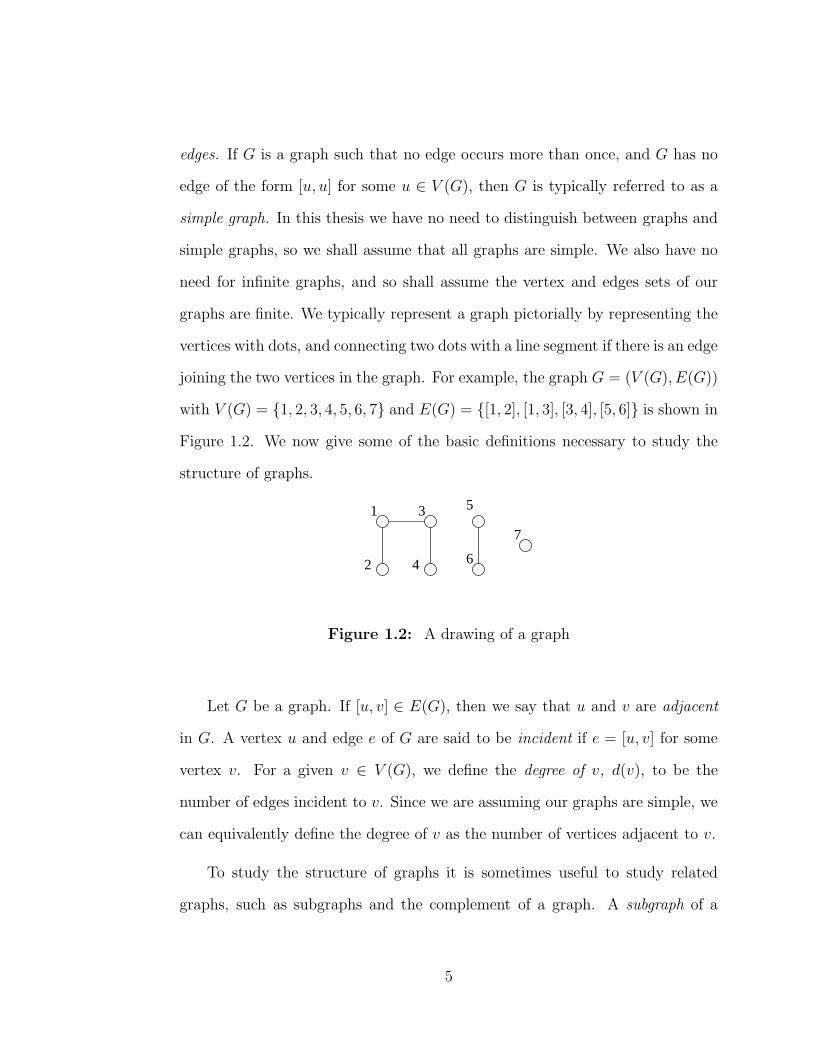
joining the two vertices in the graph. For example, the graph G = (V (G), E(G))

with V (G) = {1, 2, 3, 4, 5, 6, 7} and E(G) = {[1, 2], [1, 3], [3, 4], [5, 6]} is shown in

Figure 1.2. We now give some of the basic definitions necessary to study the

structure of graphs.

1

2 6

7

3

4

5

Figure 1.2: A drawing of a graph

Let G be a graph. If [u, v] ∈ E(G), then we say that u and v are adjacent

in G. A vertex u and edge e of G are said to be incident if e = [u, v] for some

vertex v. For a given v ∈ V (G), we define the degree of v, d(v), to be the

number of edges incident to v. Since we are assuming our graphs are simple, we

can equivalently define the degree of v as the number of vertices adjacent to v.

To study the structure of graphs it is sometimes useful to study related

graphs, such as subgraphs and the complement of a graph. A subgraph of a

5

graph G, is a graph H with V (H) ⊆ V (G) and E(H) ⊆ E(G). Given a set

S ⊆ V (G), the subgraph induced on S, G[S], is the graph with V (G[S]) = S,

and [u, v] ∈ E(G[S]) if and only if u, v ∈ S and [u, v] ∈ E(G). A graph H

is called an induced subgraph of G if H = G[S] for some S ⊆ V (G). The

complement of a graph G is the graph G, with V (G) = V (G) and [u, v] ∈ E(G)

if and only if [u, v] 6∈ E(G).

A path between vertices u and v in a graph G (sometimes called a u, v-

path) is an alternating sequence of vertices and edges of G, beginning with u

and ending with v, such that no vertex or edge is repeated, and each vertex is

incident with the edge immediately preceding and succeeding it in the sequence.

For simplicity, we typically only list the vertices of a path. The length of a path

is defined to be the number of edges in the path. The distance between vertices

u and v is defined to be the length of a shortest u, v-path. Also, a graph G

is said to be connected if there exists a u, v-path for all distinct u, v ∈ V (G).

A graph G which is not connected is called disconnected, and the maximally

connected subgraphs of G are called the connected components or components

of G. A component of order 1 is referred to as an isolated vertex.

Cycles and cliques are important graph structures that come up frequently

in chapter 5. A cycle in a graph G is an alternating sequence of vertices and

edges of G, beginning and ending with the same vertex, such that no edge is

repeated, only the first vertex is repeated, and each vertex is incident to the

edge immediately preceding and succeeding it. If all the vertices and edges of G

are contained in a cycle, we call G a cycle. The length of a cycle is the number

of edges occurring in the cycle, and a cycle of length n is called an n-cycle,

6

typically denoted by Cn. If the length of a cycle is odd or even, then we refer to

the cycle as an odd cycle or even cycle respectively. A complete graph, or clique,

on n vertices, written Kn, is a graph with n vertices, such that [u, v] ∈ E(Kn) for

all distinct u, v ∈ V (Kn). Typically the term clique is reserved for a complete

subgraph of some graph.

Another important class of graphs which come up throughout the thesis are

the bipartite graphs. A graph B is said to be bipartite if V (B) can be partitioned

into two sets X and Y , called a bipartition, such that no two vertices of X are

adjacent and no two vertices of Y are adjacent. A well known result on bipartite

graphs, which proves useful in chapter 5, is that a graph is bipartite if and only

if it contains no odd cycles. A complete bipartite graph, or biclique, is a bipartite

graph B with bipartition X ∪ Y so that [x, y] ∈ E(B) for all x ∈ X and y ∈ Y .

If |X| = r and |Y | = s, then we sometimes denote the biclique on X∪Y by Kr,s.

As with clique, the term biclique is typically reserved for a complete bipartite

subgraph of some graph. Bicliques play an important role in chapter 6 because

of their relationship with rank 1 matrices. We now turn our attention to directed

graphs.

A directed graph, or digraph, D is a set of vertices V (D), together with a set

A(D) of ordered pairs of vertices, called arcs. An orientation of a graph G is a

digraph D obtained from G by letting V (D) = V (G) and for each [u, v] ∈ E(G),

making exactly one of (u, v) or (v, u) an arc of D. Directed graphs are typically

drawn in a manner analogous to graphs, in that each vertex is represented by a

dot, and we draw an arrow from vertex u to vertex v if (u, v) is an arc of of the

digraph. Figure 1.3 shows a drawing of the digraph D = (V (D), A(D)) where

7

V (D) = {1, 2, 3, 4, 5, 6} and A(D) = {(2, 3), (3, 4), (5, 5), (4, 1), (4, 3), (5, 6)}. We

now give some of the necessary definitions and notation to study digraphs in this

thesis.

1 2

4 3 6

5

Figure 1.3: A drawing of a digraph

If (u, v) ∈ A(D), then we typically say that u “beats” v or that u “domi-

nates” v and write this as u → v. We define the outset, OD(v), of a vertex v in

D to be the set of all vertices that v dominates. That is,

OD(v) = {u ∈ V (D) : (v, u) ∈ A(D)}.

Similarly, the inset, ID(v), of a vertex v in D is the set of all vertices which

dominate v. So,

ID(v) = {u ∈ V (D) : (u, v) ∈ A(D)}.

The closed outset and closed inset of a vertex v are defined by OD[v] = OD(v)∪

{v} and ID[v] = I(v) ∪ {v} respectively. If S ⊆ V (D), then we define the

outset of S as the set of all vertices dominated by some vertex in S, written

OD(S). Equivalently, we can define the outset of S by OD(S) = ∪v∈SOD(v).

We denote by OD[S], the closed outset of S, defined by OD[S] = OD(S)∪S. The

8

inset of S and closed inset of S are defined analogously as ID(S) = ∪v∈SI(v)

and ID[S] = I(S) ∪ S respectively. When the context of which digraph we are

referring to is clear we will drop the subscript.

The out-degree of a vertex v in a digraph D, written d+D(v), is defined to

be |OD(v)|. Similarly, the in-degree of v is d−D(v) = |ID(v)|. Again, when

the context is clear, we will drop the subscript. The minimum out-degree of a

digraph D, denoted δ+(D), is defined to be δ+(D) = min{d+(v) : v ∈ V (D)}.

Similarly, the minimum in-degree of D is δ−(D) = min{d−(v) : v ∈ V (D)}. We

define the maximum out-degree and maximum in-degree of a digraph D to be the

values ∆+(D) = max{d+(v) : v ∈ V (D)} and ∆−(D) = max{d−(v) : v ∈ V (D)}

respectively.

Let D be a digraph. A subdigraph of D is a digraph D′ such that V (D′) ⊆

V (D) and A(D′) ⊆ A(D). If S ⊆ V (D), then the subdigraph induced on S is

the digraph D′ with V (D′) = S and (u, v) ∈ A(D′) if and only if u, v ∈ S and

(u, v) ∈ A(D). A digraph D′ is called an induced subdigraph of D if there exists

some S ⊆ V (D) which induces D′.

A directed path in a digraph D is an alternating sequence of vertices and arcs

of D, beginning and ending with vertices, so that no vertex or arc is repeated,

and if (u, v) is an arc in the path, the vertex immediately preceding it must be

u and the vertex immediately succeeding it must be v. A directed path which

begins at a vertex u and ends at a vertex v is called a directed u, v-path. Similar

to the undirected case, the length of a directed path is defined to be the number

of arcs in the path. If D is a directed graph so that there is a directed u, v-path

for every distinct u, v ∈ V (D), then we say D is strongly connected. If D is not

9

strongly connected, then the maximal strongly connected subdigraphs of D are

called the strong components of D.

A directed cycle in a digraph D is an alternating sequence of vertices and

arcs of D which begin and end with the same vertex, repeat no vertices or edges,

and if (u, v) is an arc in the cycle, then the vertex immediately preceding it must

be u and the vertex immediately succeeding it must be v. Similar to undirected

cycles, the length of a directed cycle is the number of arcs in the cycle. A

directed cycle of length n is referred to as a directed n-cycle. Also, as before,

an n-cycle is called a directed odd cycle or directed even cycle if n is odd or even

respectively. If it is clear that we are dealing with a directed context, we will

simply refer to directed cycles and directed paths as cycles and paths.

To study the structure of graphs and digraphs, it is useful to have a concept

of isomorphism in graphs and digraphs. An isomorphism of graphs G and H

is a bijective function φ : V (G) → V (H) such that [u, v] ∈ E(G) if and only

if [φ(u), φ(v)] ∈ E(H). That is, a graph isomorphism is an adjacency preserv-

ing bijection. We say that two graphs are isomorphic if there exists a graph

isomorphism between them. Similarly, we define an isomorphism of digraphs D

and D′ to be a bijection φ : V (D) → V (D′) such that (u, v) ∈ A(D) if and

only if (φ(u), φ(v)) ∈ A(D′). That is, a digraph isomorphism is a dominance

preserving bijection. An isomorphism from a graph to itself (digraph to itself)

is called a graph automorphism (digraph automorphism). We now look at the

class of digraphs studied most in this thesis.

1.3 Tournament basics

10

In this section we review some of the basic terminology and properties of

tournaments. A tournament T is a complete asymmetric digraph. That is, for

every two distinct u, v ∈ V (T ), either (u, v) ∈ A(T ) or (v, u) ∈ A(T ), but not

both, and (v, v) 6∈ A(T ) for all v ∈ V (T ). A tournament with n vertices, is called

an n-tournament. Equivalently, some define an n-tournament as an orientation

of the complete graph Kn. An example of a 5-tournament is shown in Figure 1.4.

Figure 1.4: A 5-tournament

In studying tournament structure, we often want to look at subtournaments

and the dual of a tournament. Given a tournament T , and S ⊆ V (T ), a subtour-

nament of T is the tournament T [S], with V (T [S]) = S, and (u, v) ∈ A(T [S]) if

and only if u, v ∈ S and (u, v) ∈ A(T ). That is, T [S] is the subdigraph induced

on S. Also, for a vertex v ∈ V (T ) or a set of vertices S, we define the subtour-

naments T −v and T −S to be the tournaments T [V (T )−{v}] and T [V (T )−S]

11

respectively. The dual of T is the tournament T r, with V (T r) = V (T ) and

(u, v) ∈ A(T r) if and only if (v, u) ∈ A(T ). We define the dual of a digraph in

the same way, and use the same notation.

One of the most famous results about tournaments is Landau’s Theorem.

The list of out-degrees of the vertices of a tournament is called its score sequence.

In 1953 Landau characterized which lists of n positive integers could be the score

sequence of some tournament.

Theorem 1.1 (Landau’s Theorem) Let s1, s2, . . . , sn be a non-decreasing se-

quence of positive integers. This list is the score sequence for some n-tournament

if and only ifk∑

i=1

si ≥(

k

2

)

for 1 ≤ k ≤ n − 1 andn∑

i=1

si =

(

n

2

)

.

The necessity in Landau’s Theorem is easy to see. Any n-tournament must

have an arc between every two vertices, and hence(

n

2

)

arcs. Further, every sub-

tournament of an n-tournament on k vertices will have(

k

2

)

arcs. The argument

follows by counting arcs in subtournaments in this way, and by counting them

as the sum of the out-degrees of a subset of vertices. The sufficiency in Landau’s

Theorem has been proved in many ways, by many people. It has been proven by

using classic combinatorial methods, using majorization of vectors, using posets,

using network flows, and even using Hall’s Theorem. Some of the many authors

of these proofs include Landau, Ryser, Reid, Thomassen, Fulkerson, and Bang

and Sharp. For a full proof of Landau’s Theorem the reader is referred to [50].

12

Another classic theorem on tournaments involves Hamiltonian paths. Given

a digraph D, a Hamiltonian path is a path which contains every vertex of D.

By taking a path of maximum length in a tournament, one can show, via the

complete asymmetry of the tournament, that there is no vertex not on the path

and it is hence Hamiltonian. We discuss an analogous result about cycles in

strong tournaments below. We now state this theorem.

Theorem 1.2 Every tournament contains a Hamiltonian path.

In this thesis, we are often concerned with when one set in a tournament

completely dominates another. Let T be a tournament and S, S ′ ⊆ V (T ). If

for every u ∈ S and v ∈ S ′, u → v, then we write S ⇒ S ′. In the case

where S = {u} (S ′ = {v}), we write u ⇒ S ′ (S ⇒ v) rather than {u} ⇒ S ′

(S ⇒ {v}). A vertex s ∈ V (T ) such that s ⇒ V (T )−{s} is called a transmitter.

A vertex t ∈ V (T ) such that V (T ) − {t} ⇒ t is called a receiver. The concept

of one set completely dominating another plays an important part in our study

of tournaments and tournament matrices, as it corresponds to large blocks of

ones in the adjacency matrix. Tournaments with transmitters and receivers also

play a part as special cases of some of our results. In particular, when studying

tournaments which are not strongly connected, tournaments with transmitters

or receivers are important special cases.

As with digraphs, we define a tournament T to be strongly connected if for

any two vertices u, v ∈ V (T ) there is a directed path in T from u to v and

another from v to u, and a strong component of a tournament to be a maximal

strongly connected subtournament. We sometimes refer to a strongly connected

13

tournament as a strong tournament. We note that a single vertex is trivially

strongly connected, and that a 2-tournament has exactly one arc, and hence

cannot be strongly connected. So, the smallest non-trivial strong component

which a tournament could have is the 3-cycle. Strong tournaments have been

characterized in terms of their score sequences by replacing the inequalities in

Landau’s Theorem with strict inequalities. The following two theorems are well

known, useful results on the structure of tournaments.

Theorem 1.3 Let T be a strong n-tournament, and let v ∈ V (T ). Then v is

contained on a cycle of length k for k = 3, . . . , n.

Theorem 1.4 Let T be a tournament which is not strongly connected. Then

V (T ) can be partitioned by the strong components of T , and these components

can be labeled T1, T2, . . . , Tm such that Ti ⇒ Tj if and only if i < j.

The strong components T1 and Tm in the previous theorem are called the

initial and terminal strong components of T respectively. The above result has

also been stated as “The condensation of a tournament is transitive.” A tran-

sitive tournament is one in which for all u, v, w ∈ V (T ), if u → v and v → w,

then u → w. There are several equivalencies for the definition of a transitive

tournament. The two others we will most frequently use are that the vertices

can be labeled v1, v2, . . . , vn such that vi → vj if and only if i < j, and that

0, 1, 2, . . . , n − 1 is the score sequence of T . We also note that the transitive

tournament on n vertices is unique up to isomorphism.

The condensation of a tournament T is typically defined to be the tourna-

ment T ′ obtained by representing each strong component of T with a vertex of

14

T ′, and letting u → v if and only if for the corresponding strong components

Tu and Tv we have that Tu ⇒ Tv. Theorem 1.4 above, with this definition, may

also be stated as “The condensation of a tournament is always a transitive tour-

nament.” In this thesis we will adopt the following, more versatile definition of

condensation. Let T be a tournament, and suppose we can partition the vertices

of T as S1, S2, . . . , Sm such that for all i 6= j either Si ⇒ Sj or Sj ⇒ Si. We de-

fine the condensation of T , with respect to this partition, to be the tournament

T ′ with V (T ) = {v1, v2, . . . , vm} with vi → vj in T ′ if and only if Si ⇒ Sj in T .

In the study of tournaments, the extreme examples of many problems tend to

be transitive tournaments and regular tournaments. We discussed the transitive

tournaments above. A regular tournament is one in which every vertex has

the same out-degree. Consequently, every vertex in a regular tournament has

the same in-degree. Thus, for every regular n-tournament, n is odd and the

out-degree and in-degree of every vertex is n−12

. While there are no regular n-

tournaments for n even, we do have an analogous tournament. A near regular

tournament is a tournament in which the out-degrees of any two vertices differs

by at most one. By some counting arguments, one can show that if T is a near

regular n-tournament, then n is even, exactly half of the vertices have out-degree

n2

and exactly half of the vertices have out-degree n2− 1.

Up to isomorphism, there is only one transitive n-tournament, however there

can be many non-isomorphic regular n-tournaments. To better study regular

tournaments we often turn to the class of rotational tournaments. Rotational

tournaments have a nice structure which makes them somewhat easier to work

with, and while not all regular tournaments are rotational, there are typically a

15

large number of rotational n-tournaments for a given n. This makes rotational

tournaments a nice class of regular tournaments to start with when studying

questions about regular tournaments. We give the construction for rotational

tournaments below.

Choose an odd positive integer n, and let S be a subset of {1, 2, . . . , n − 1}

of order n−12

such that i ∈ S if and only if −i (mod n) is not in S. Construct a

digraph T on the vertices {0, 1, 2, . . . , n− 1} with i → j in T if and only if j − i

(mod n) is in S. Since x is in S if and only if −x (mod n) is not, we have that

for any two distinct i, j ∈ V (T ) exactly one of j − i (mod n) or i − j (mod n)

is in S. So we have that i → j or j → i, but not both. Further, since 0 6∈ S, T

has no arcs of the form (i, i). Thus T is a tournament. We call T a rotational

tournament with symbol S.

To see that rotational tournaments are regular choose any vertex i. Then,

O(i) = {i + j (mod n) : j ∈ S}, and so each vertex has the same out-degree.

Another important property of rotational tournaments is that they are vertex

transitive. A vertex transitive tournament T is one in which for every two

vertices u, v in T , there exists an automorphism of T that maps u to v. Given

a rotational tournament T with symbol S, pick i, j ∈ V (T ), and let k ≡ j − i

(mod n). Consider the function φ, defined by φ : a 7→ a + k (mod n). It is easy

to see that φ is a bijection. Further, if a → b in T , then b − a (mod n) is in S,

and φ(b)−φ(a) ≡ b+k− (a+k) ≡ b−a (mod n) which is in S, so φ(a) → φ(b),

and φ is an automorphism of T . Finally, φ(i) = i + (j − i) = j, so φ is an

automorphism which maps i to j, and since i and j were chosen arbitrarily, T

is vertex transitive.

16

An important class of rotational tournaments which come up frequently in

this thesis are the quadratic residue tournaments. Recall from number theory

that an integer a is called a quadratic residue modulo n if there exists some

x such that a ≡ x2 (mod n). For any given odd prime p, we know that there

are p−12

quadratic residues modulo p. Further, given a prime p such that p ≡ 3

(mod 4), we know that i is a quadratic residue if and only if −i is not. (For a

proof of this, and more on quadratic residues see [49].) So, given a prime p ≡ 3

(mod 4), the quadratic residues modulo p form a symbol for a rotational p-

tournament. We call this tournament the quadratic residue tournament of order

p, written QRp. An important, and well known property of quadratic residue

tournaments is that they are arc-transitive. An arc-transitive tournament T is

one in which for any two arcs (i, j) and (h, k) in T , there exists an automorphism

of T which maps i to h and j to k. We now state and prove this property for

completeness.

Theorem 1.5 Quadratic residue tournaments are arc-transitive.

Proof: Let p ≡ 3 (mod 4) be a prime, and choose arc (i, j) and (h, k) in

QRp. Let a = (k − h)(j − i)−1 and b = (hj − ki)(j − i)−1. Note a is a quadratic

residue since k − h and j − i are quadratic residues, and the set of quadratic

residues modulo p form a group under multiplication. Define the function f by

f : x 7→ ax + b (mod p). Since V (QRp) = Zp is a field, f is a bijection from

V (QRp) to V (QRp). To see that f is an automorphism, pick (x, y) ∈ A(QRp).

Then (y − x) is a quadratic residue modulo p, and

f(y) − f(x) = ay + b − (ax + b) = ay − ax = a(y − x).

17

Since a and (y − x) are quadratic residues, a(y − x) is a quadratic residue, and

so f(x) → f(y). So, f preserves dominance and is hence and automorphism.

Also,

f(i) = ai + b

= ((k − h)(j − i)−1)i + (hj − ki)(j − i)−1

= (ki − hi + hj − ki)(j − i)−1

= h(j − i)(j − i)−1

= h,

and

f(j) = aj + b

= ((k − h)(j − i)−1)j + (hj − ki)(j − i)−1

= (kj − hj + hj − ki)(j − i)−1

= k(j − i)(j − i)−1

= k

Thus, QRp is arc-transitive.

The arc-transitivity of quadratic residue tournaments tells us that the tour-

nament induced on O(u)∩O(v) is the same for any two distinct vertices u, v in

QRp. In particular, this tells us that |O(u) ∩ O(v)| is the same for all distinct

u, v ∈ V (QRp). Tournaments with this property are called doubly regular tour-

naments. That is, a tournament T is called a doubly regular tournament if for

all distinct u, v ∈ V (T ), |O(u) ∩ O(v)| = k, for some given k.

18

A doubly regular tournament with |O(u) ∩ O(v)| = k for all distinct u, v

is also a regular tournament on 4k + 3 vertices with d+(v) = 2k + 1 for all

vertices v. Doubly regular tournaments have many nice properties. In particular,

they form extremal cases for many problems in tournaments. While it is not

certain, they also appear to be good candidates for extremal cases in some of

the problems posed in this thesis. For instance, it is our current belief that if

a tournament is going to be the digraph of an orthogonal matrix, the smallest

non-trivial example will be doubly regular. (In fact, the only known example is

the 3-cycle, which is doubly regular with k = 0.) We also believe that doubly

regular tournaments will be the optimal choices when extending tournaments to

create larger tournaments with small Boolean rank. For more on doubly regular

tournaments, the reader is referred to Reid and Brown, [10].

1.4 Domination basics

Given a digraph D, and a set S ⊆ V (D), we say that S is a dominating

set in D if O[S] = V (D). In this section we discuss some of the background

on domination in digraphs and tournaments, and how it relates to the problems

studied in this thesis. Domination in tournaments has been studied by many

people. The original problem appears to be a problem of Schutte, in which he

asks, “For a given k, what is the least n so that there exists an n-tournament

T such that for all S ⊆ V (T ) with |S| = k, there exists a vertex v ∈ V (T )

with v ⇒ S?” Taking the asymmetry of tournaments into account, one can

see that if there is no such vertex for a set S, then S is a dominating set. The

order of a smallest dominating set in D is called the domination number of

D, written γ(D). So, answering Schutte’s problem is equivalent to finding a

19

smallest n-tournament T with γ(T ) > k.

A property related to domination that we will discuss in chapter 6 is irre-

dundance. An irredundant set in a digraph D is a set S such that for all u ∈ S,

there exists a vertex v ∈ V (D) such that v ∈ O[u]−O(S). The size of a smallest

maximal irredundant set in a digraph D is called the lower irredundance number

of D, written ir(D). The size of a largest irredundant set is called the upper

irredundance number, written IR(D). Similarly, the size of a largest minimal

dominating set is called the upper domination number, written Γ(D). A recent

treatment and collection of results on domination and irredundance in tourna-

ments can be found in Hedetniemi, Hedetniemi, McRae, and Reid [34]. The

following useful result of basic bounds on γ, Γ, ir and IR is taken from their

paper.

Theorem 1.6 [34] For every tournament T ,

(i) ir(T ) ≤ γ(T ) ≤ ∆+(T );

(ii) ir(T ) ≤ γ(T ) ≤ Γ(T ) ≤ IR(T );

(iii) γ(T ) ≤ n − ∆+(T );

(iv) γ(T ) ≤ δ−(T ) + 1.

As mentioned in the previous section, doubly regular tournaments form

extremal examples for several problems, and appear to be extremal examples for

some of the problems in this thesis. This also appears to be true when looking

for tournaments with large domination numbers. For instance, the smallest

tournament with domination number 2 is the 3-cycle. The smallest tournament

20

such that every set of 2 vertices is dominated by a third, and hence the smallest

tournament with domination number 3, is QR7 (note this is the only doubly

regular 7-tournament and is hence the unique 7-tournament with domination

number 3). It can also be verified that the smallest tournament with domination

number 4 is QR19 (see [34]). Some of these examples prove quite useful when

we begin relating domination in tournaments to properties in the corresponding

tournament matrices.

One way in which we will relate domination to matrix properties, especially

in chapters 2 and 4 is by studying the structure of dominant pairs in a tourna-

ment. A dominant pair in a tournament is a dominating set of order 2. Given

a tournament T , the domination graph of T is the graph dom(T ) on the same

vertices as T with [u, v] ∈ E(dom(T )) if and only if {u, v} form a dominant pair

in T . As mentioned, the domination graphs of tournaments were introduced by

Merz, Lundgren, Reid, and Fisher in [44], and have since been characterized in

a series of papers.

Our study of the domination graphs of tournaments comes from their rela-

tion to the competition graphs of tournaments. Given a digraph D, the com-

petition graph of D is the graph comp(D) on the same vertices as D with

[u, v] ∈ E(comp(D)) if and only if u 6= v and there exists some w ∈ V (D)

such that u → w and v → w. Recall from the asymmetry of tournaments, that

two vertices will dominate a tournament if and only if there does not exist a

vertex which dominates them both. This is the main idea behind the following

theorem of Merz et. al..

21

Theorem 1.7 [44] The complement of the competition graph of a tournament

is the domination graph of its dual.

If D is a digraph, and M its adjacency matrix, then for i 6= j, the i, j entry

of MM> will be non-zero if and only if row i and row j share a common non-zero

entry. That is, the i, j entry of MM> will be non-zero if and only if vertex i and

vertex j compete in D. So, the non-zero, off diagonal entries of the adjacency

matrix of comp(D) are in direct correspondence with those of MM>. This

relationship together with the above result is the main correspondence between

domination in tournaments and the matrix properties discussed in chapter 2.

We use Merz et. al.’s characterization of the domination graphs of tourna-

ments in chapter 4, along with a characterization of separable matrices in terms

of the competition graphs of the corresponding digraphs, to characterize exactly

which tournament matrices are separable. In chapter 5 we use this characteri-

zation as a jumping off point for our characterization of the domination graphs

of complete paired comparison digraphs. We state the necessary conditions of

the characterization here, but first recall the following definitions.

Recall that a tree is a connected acyclic graph. A caterpillar is a tree such

that the removal of all pendant vertices results in a path. Each caterpillar has

a path of maximum length called a spine. A spiked cycle is a graph such that

the removal of all pendant vertices results in a cycle. If the cycle in a spiked

cycle is odd, then we call it a spiked odd cycle. Note, a spiked cycle need not

have pendants. So, cycles form a subclass of spiked cycles, and odd cycles form

a subclass of spiked odd cycles.

22

Figure 1.5: An example of a spiked cycle and a caterpillar

Theorem 1.8 [44] The domination graph of a tournament is either a caterpil-

lar or a spiked odd cycle.

The sufficient conditions for the characterization of domination graphs of

tournaments vary depending on connectedness restrictions and can be found

in [31], [43], [45], and [46]. We now turn to some necessary background on

(0, 1)-matrices and matrix theory.

1.5 Matrix basics

In this section we cover some basic definitions and background on (0, 1)-

matrices. First, we introduce the notation we shall use for discussing matrices

and vectors. Let M be a matrix. We denote the i, j entry of M by Mi,j. We

use Mi• to represent the ith row of M and Mi to represent the ith column of M .

If v is a vector, then we let vi denote the ith entry of the vector.

A (0, 1)-matrix is a matrix whose every entry is a 0 or 1. We concern

ourselves with square (n × n) (0, 1)-matrices in this thesis. Any square (0, 1)-

matrix can be considered the adjacency matrix of some digraph. Let D be a

23

digraph with V (D) = {1, 2, . . . , n}. The adjacency matrix of D is the n × n

(0, 1)-matrix M defined by

Mi,j =

{

1 if (i, j) ∈ A(D),

0 if (i, j) 6∈ A(D).

In chapters 2, 3, and parts of chapters 4 and 6 we are interested in the

patterns of matrices. Given a matrix A, with arbitrary entries, the pattern of A

is the (0, 1)-matrix M obtained from A by letting

Mi,j =

{

1 if Ai,j 6= 0,

0 if Ai,j = 0.

This has also been called a non-zero pattern by some authors. The digraph D

whose adjacency matrix is the pattern of a matrix A is called the digraph of A.

If M is the pattern of a matrix A, or D the digraph of A, then we sometimes

say that M and D support A.

Just as tournaments are an important class of digraphs to study, tournament

matrices give rise to several interesting problems in the study of (0, 1)-matrices.

A tournament matrix is the adjacency matrix of a tournament. By the complete

asymmetry of tournaments, one could also define a tournament matrix to be a

square (0, 1)-matrix M with 0s on the diagonal and Mi,j = 1 if and only if

Mj,i = 0. A third equivalent definition of tournament matrices is a square

(0, 1)-matrix M such that M + M> = J − I, where J is a matrix of all 1s, and

I the identity matrix.

Some other important classes of matrices which come up are the zero ma-

trices, the class of matrices Jm×n, and the permutation matrices. An m×n zero

24

matrix, Om,n, is an m × n matrix in which every entry is a 0. If m = n, we will

simply write On, or if the dimensions are clear from context, O. We will write a

vector of all zeros as 0. The m×n matrix Jm,n is an m×n matrix of ones. Again,

if m = n, we will simply write Jn, or J if the dimensions are clear from con-

text. We write a vector of all ones as 1. Given a bijection φ from {1, . . . , n} to

{1, . . . , n}, a permutation matrix is a matrix P with Pi,φ(i) = 1 for i = 1, . . . , n,

and Pi,j = 0 otherwise. A well known property of permutation matrices is that

left multiplying a matrix A by a permutation matrix P> will reorder the rows

of A according to the bijection corresponding to P , and right multiplying A by

P will reorder the columns according to the bijection corresponding to P .

If M is the adjacency matrix of some digraph D, and P a permutation ma-

trix, then left and right multiplying M by P> and P respectively, results in

the adjacency matrix of a digraph isomorphic to D. Left and right multiply-

ing M by permutation matrices P and Q results in a permutation equivalent

matrix. Permutation equivalent matrices do not necessarily correspond to iso-

morphic digraphs, but are important for some matrix properties. We study the

permutation equivalence of tournaments in chapter 4.

We denote the standard Euclidean inner product of two vectors x and y by

〈x,y〉. That is, for column vectors x and y, 〈x,y〉 = x>y. We say two vectors x

and y are orthogonal if 〈x,y〉 = 0. An n× n matrix M is said to be orthogonal

if MM> = M>M = I. So, if M is orthogonal, 〈Mi•, Mj•〉 = 0 and 〈Mi, Mj〉 = 0

for all i 6= j, and∑n

j=1 M2i,j =

∑n

i=1 M2i,j = 1, for any i, j.

Two less traditional matrix concepts which arise in chapter 6 are comple-

ments of matrices, and the idea of one matrix being less than another. Given a

25

(0, 1)-matrix, M , we define the complement of M to be the matrix M c, where

M ci,j = 1 if and only if Mi,j = 0. Given two matrices A and M , we say that

A ≤ M if they have the same dimensions and for all i, j, Ai,j ≤ Mi,j. Equiva-

lently, for vectors x and y, we say x ≤ y if xi ≤ yi for all i. We define these

since (0, 1)-matrices and vectors tie in closely with sets when we begin dealing

with Boolean arithmetic in chapter 6. Also, for a set S and subset W of S, we

will also write the complement of W in S as W c.

26

2. Quadrangular Tournaments

2.1 Definitions and background

Recall that an n × n matrix M is defined to be orthogonal if MM> =

M>M = I, where I is the n × n identity matrix. In this chapter we introduce

a basic necessary condition for a digraph to support an orthogonal matrix, and

study the tournaments which meet this condition. Our condition is derived

from combinatorial orthogonality, which originally appeared in a matrix context

in [5]. Given two n-vectors x = (x1, x2, . . . , xn) and y = (y1, y2, . . . , yn) with

entries from any field, we say that x and y are combinatorially orthogonal if

|{i : xiyi 6= 0}| 6= 1. That is, they do not share exactly 1 non-zero entry. We say

a matrix M is combinatorially orthogonal if every two rows are combinatorially

orthogonal and every two columns are combinatorially orthogonal.

To see that this is in fact a necessary condition for a matrix to be orthog-

onal, let M be a matrix with rows Mi• and Mj• which are not combinatorially

orthogonal (a similar argument holds for columns). Then Mi• and Mj• have

exactly one non-zero entry in common, and so 〈Mi•, Mj•〉 is just the product

of these two entries and hence, not zero. As any two rows (or columns) of an

orthogonal matrix must be orthogonal, we see that combinatorial orthogonality

is a necessary condition for a matrix to be orthogonal. Further, since combi-

natorial orthogonality only concerns itself with whether an entry is non-zero or

not, combinatorial orthogonality is a necessary condition for a (0, 1)-matrix to

be the pattern of an orthogonal matrix.

27

A digraph D is called quadrangular if for all distinct u, v ∈ V (D), |O(u) ∩

O(v)| 6= 1 and |I(u) ∩ I(v)| 6= 1. If we only require the restriction on the

outsets or insets separately, we say D is out-quadrangular or in-quadrangular

respectively. Figure 2.1 shows an example of a quadrangular digraph. Note that

Figure 2.1: A Quadrangular Digraph

if A is the adjacency matrix of a digraph, and Ai• and Aj• two rows of A which

correspond to vertices u and v respectively, then 〈Ai•, Aj•〉 = |O(u) ∩ O(v)|.

Similarly, the inner product of two columns is equal to the size of the intersection

of the insets of the corresponding vertices. So, D is a quadrangular digraph, if

and only if its adjacency matrix is a combinatorially orthogonal matrix. Thus,

quadrangularity is a necessary condition for a digraph to support an orthogonal

matrix.

Many of the results in this chapter show that, in certain classes of tour-

naments, there is a relationship between quadrangularity and the domination

number of the tournament or a subtournament. For example, Theorems 2.1,

2.8, and 2.19 all exhibit this relationship. We begin by examining tournaments

which are not strongly connected. We see that in this case quadrangularity of

the tournament can be reduced to the question of quadrangularity in a strong

28

subtournament, or a bound on the domination number of a subtournament. We

then look at cases where we have restrictions on the out-degrees and in-degrees

of the tournament. We finish the chapter by characterizing the orders for which

a quadrangular tournament exists.

2.2 Tournaments which are not strongly connected

Our first result of this section classifies quadrangular tournaments with a

transmitter and a receiver by a bound on the domination number of a subtour-

nament.

Theorem 2.1 Let T be a tournament on 3 or more vertices with a transmitter

s and receiver t. Then T is quadrangular if and only if both γ(T − {s, t}) > 2

and γ((T − {s, t})r) > 2.

Proof: Let T be a tournament with a transmitter s and receiver t. Suppose

that both γ(T−{s, t}) > 2 and γ((T−{s, t})r) > 2. Then, E(dom(T−{s, t})) =

E(dom((T −{s, t})r)) = ∅. Thus the competition graphs of both T −{s, t} and

(T − {s, t})r are complete. That is, for all x, y ∈ V (T ) − {s, t} there exist

w, z ∈ V (T ) such that w → x, w → y, x → z and y → z. Pick distinct

u, v ∈ V (T ). We consider three cases.

Case 1: Suppose u, v 6∈ {s, t}. Then, as noted before, there exist vertices

w, z ∈ V (T − {s, t}) so that z ∈ O(u) ∩ O(v) and w ∈ I(u) ∩ I(v). Also,

s ∈ O(u)∩O(v) and t ∈ I(u)∩I(v). So, |O(u)∩O(v)| ≥ 2 and |I(u)∩I(v)| ≥ 2.

Case 2: Now assume that one of u, or v is t, say u = t. Since O(t) = ∅,

O(t)∩O(v) = ∅, so |O(t)∩O(v)| = 0. Also, I(t) = V (T )−{t}, so I(t)∩ I(v) =

I(v). If v = s, then I(v) = ∅, and |I(t) ∩ I(v)| = 0. So, suppose v 6= s. Since

29

γ(T −{s, t}) ≥ 3, Theorem 1.6 gives us that 2 ≤ γ(T −{s, t}) ≤ δ−(T −{s, t}).

Thus, d−(v) ≥ 2, and since I(v) ⊆ I(t), |I(t) ∩ I(v)| = d−(v) ≥ 2 as desired.

Case 3: Now, assume that one of u, v is s, say u = s. Since I(s) = ∅, I(s)∩I(v) =

∅, so |I(s) ∩ I(v)| = 0. Also, since O(s) = V (T ) − {s}, O(s) ∩ O(v) = O(v).

The case where v = t is covered in case 2, so assume v 6= t. Since γ((T −

{s, t})r) ≥ 3, Theorem 1.6 gives us that 2 ≤ γ((T−{s, t})r) ≤ δ−((T−{s, t})r) =

δ+(T − {s, t}). Thus, d+(v) ≥ 2, and since s is a transmitter, O(v) ⊆ O(s), so

|O(s) ∩ O(v)| = d+(v) ≥ 2.

Conversely assume that T is a quadrangular tournament with both a trans-

mitter s and receiver t. If u, v ∈ V (T ) − {s, t}, then s ∈ O(u) ∩ O(v),

and t ∈ I(u) ∩ I(v). So, since T is quadrangular, |O(u) ∩ O(v)| ≥ 1 and

|I(u) ∩ I(v)| ≥ 1, there must exist vertices w, z in T − {s, t} such that

z ∈ O(u) ∩ O(v) and w ∈ I(u) ∩ I(v). Since w beats u and v they cannot be a

dominant pair in T −{s, t} and since u and v beat z they cannot be a dominant

pair in (T − {s, t})r. Thus, E(dom(T − {s, t})) = E(dom((T − {s, t})r)) = ∅.

Equivalently, γ(T − {s, t}) > 2 and γ((T − {s, t})r) > 2. This completes our

proof.

From Theorem 1.6, and Theorem 2.1 we get the following corollary which

allows for a quick check to see if a tournament with both a transmitter and a

receiver is quadrangular.

Corollary 2.2 Let T be a tournament on 3 or more vertices with a transmitter s

and receiver t. If T is quadrangular, then δ+(T−{s, t}) ≥ 2 and δ−(T−{s, t}) ≥

2.

30

The following results characterize quadrangular tournaments in the case

where the tournament has a transmitter or receiver, but not both, by a bound

on the domination number of a subtournament.

Theorem 2.3 Let T be a tournament with a transmitter s and no receiver.

Then T is quadrangular if and only if, γ(T − s) > 2, T − s is out-quadrangular,

and δ+(T − s) ≥ 2.

Proof: First suppose that γ(T − s) > 2, T − s is out-quadrangular, and

δ+(T − s) ≥ 2. Pick distinct u, v ∈ V (T ). First suppose that u, v ∈ V (T )−{s}.

Since γ(T − s) > 2 there exists x ∈ V (T )−{s} such that x → u and x → v. So,

s, x ∈ I(u)∩I(v) and so |I(u)∩I(v)| ≥ 2. Also, since T −s is out-quadrangular,

|O(u)∩O(v)| 6= 1. Now, suppose that one of u, v is s, say u = s. Since I(s) = ∅,

|I(s) ∩ I(v)| = 0. Also, since δ+(T − s) ≥ 2, |O(s) ∩ O(v)| = |O(v)| ≥ 2, Thus,

T − s is quadrangular as desired.

Now, assume that T is quadrangular. Since O(s) = V (T ) − {s}, |I(u) ∩

I(v)| ≥ 1 for all distinct u, v ∈ V (T ) − {s}. Since T is quadrangular this

means we must have |I(u) ∩ I(v)| ≥ 2 for each u, v ∈ V (T ) − {s}. Thus, for all

u, v ∈ V (T ) − {s}, there must exist some x ∈ V (T ) − {s} such that x → u and

x → v. So, γ(T − s) > 2. Since T has no receiver, |O(v)| ≥ 1 for all v ∈ V (T ).

Since O(s)∩O(v) = O(v) for all v ∈ V (T )−{s}, and T is quadrangular, we must

then have that d+(v) = |O(v)| = |O(s)∩O(v)| ≥ 2. Thus, δ+(T − s) ≥ 2. Now,

pick distinct u, v ∈ V (T ) − {s}. Since T is quadrangular, |O(u) ∩ O(v)| 6= 1, so

T − s is out-quadrangular.

If T is a tournament with a receiver and no transmitter, then it is the dual of

31

a tournament with a transmitter and no receiver. A tournament is quadrangular

if and only if its dual is, so by Theorem 2.3, T is quadrangular if and only if

γ((T − t)r) > 2, (T − t)r is out-quadrangular and δ+((T − t)r) ≥ 2. Since

(T − t)r being out-quadrangular is equivalent to T − t being in-quadrangular,

and δ+((T − t)r) = δ−(T − t) we get the following corollary.

Corollary 2.4 Let T be a tournament with a receiver t and no transmitter.

Then T is quadrangular if and only if γ((T − t)r) > 2, T − t is in-quadrangular,

and δ−(T − t) ≥ 2.

Theorem 1.6 together with Theorem 2.3 and Corollary 2.4 give analogous

results to Corollary 2.2. Namely that if T is a quadrangular tournament with a

transmitter s and no receiver (receiver t and no transmitter), then δ+(T −s) ≥ 2

and δ−(T − s) ≥ 2 (δ+(T − t) ≥ 2 and δ−(T − t) ≥ 2). We finish this section by

characterizing quadrangular tournaments with no transmitter or receiver which

are not strongly connected in terms of properties of their initial and terminal

strong components.

Theorem 2.5 Let T be a tournament with no transmitter or receiver which

is not strongly connected. Then T is quadrangular if and only if the initial

strong component T1 is in-quadrangular with δ−(T1) ≥ 2 and the terminal strong

component Tm is out-quadrangular with δ+(Tm) ≥ 2.

Proof: Let T be a tournament with no transmitter or receiver, which is

not strongly connected. Suppose that T1 is in-quadrangular with δ−(T1) ≥ 2,

and that Tm is out-quadrangular with δ+(Tm) ≥ 2. Note that since T has no

32

transmitter or receiver, T1 and Tm must contain at least 3 vertices each. Pick

distinct u, v ∈ V (T ). We consider 5 cases.

Case 1: Suppose that u and v are in neither T1 nor Tm. Every vertex of T1

beats every vertex in T − T1 and every vertex of Tm is beaten by every vertex

of T − Tm. So,

|O(u) ∩ O(v)| ≥ |V (Tm)| ≥ 3 and |I(u) ∩ I(v)| ≥ |V (T1)| ≥ 3.

Case 2: Suppose that both u, v ∈ T1. Then, since T1 is in-quadrangular, |I(u)∩

I(v)| 6= 1. Also, u and v beat every vertex in T − T1, in particular, V (Tm) ⊆

O(u) ∩ O(v). Thus,

|O(u) ∩ O(v)| ≥ |V (Tm)| ≥ 3.

Case 3: Suppose that both u, v ∈ V (Tm). Then, since Tm is out-quadrangular,

|O(u) ∩ O(v)| 6= 1. Also, |I(u) ∩ I(v)| ≥ |V (T1)| ≥ 3.

Case 4: Suppose that u ∈ V (T1) and v 6∈ V (T1). Since v 6∈ V (T1) we know

that I(u) ⊆ V (T1) ⊆ I(v) and so I(u) ∩ I(v) = I(u). So, since δ−(T1) ≥ 2,

|I(u) ∩ I(v)| = |I(u)| = d−(u) ≥ 2. Also, since u ∈ V (T1) and v 6∈ V (T1),

we know that O(v) ⊆ O(u). Thus, O(u) ∩ O(v) = O(v). If v 6∈ V (Tm), then

V (Tm) ⊆ O(v), and so |O(u)∩O(v)| ≥ |V (Tm)| ≥ 3. So, assume that v ∈ V (Tm).

Then |O(u) ∩ O(v)| = |O(v)| = d+(v) ≥ 2.

Case 5: Suppose that u ∈ V (Tm) and v 6∈ V (Tm). Since v 6∈ V (Tm), O(u) ⊆

V (Tm) ⊆ O(v), and so O(u) ∩ O(v) = O(u). So, since δ+(Tm) ≥ 2, |O(u) ∩

O(v)| = |O(v)| ≥ 2. Now, if v ∈ V (T1) then as in case 4, |I(u) ∩ I(v)| ≥ 2. So,

33

assume that v 6∈ V (T1). Then, every vertex in T1 beats both u and v, and so

|I(u) ∩ I(v)| ≥ |V (T1)| ≥ 3.

Now, assume that T is quadrangular. Since T is quadrangular, if u, v ∈

V (T1), then |I(u) ∩ I(v)| 6= 1, so T1 is in-quadrangular. Also, since T is quad-

rangular, if u, v ∈ V (Tm) then |O(u)∩O(v)| 6= 1, and so Tm is out-quadrangular.

Now, pick u ∈ V (T1) and v ∈ V (Tm). Then, O(u) ∩ O(v) = O(v), and

I(u) ∩ I(v) = I(u). Since T has no receiver, d+(v) ≥ 1, and so we must have

that d+(v) = |O(v)| = |O(u) ∩ O(v)| ≥ 2. Thus, δ+(Tm) ≥ 2. Also, since T has

no transmitter, d−(u) ≥ 1, and so d−(u) = |I(u)| = |I(u) ∩ I(v)| ≥ 2. Thus,

δ−(T1) ≥ 2. These are exactly the conditions from the theorem statement, and

so the result follows.

In studying tournaments which are quadrangular, the previous results allow

us to restrict our attention to strongly connected tournaments. Beyond this,

as we will see in Chapter 4, a necessary condition for a tournament to be the

digraph of an orthogonal matrix is to be strongly connected.

2.3 Tournaments with given minimum degrees

We now look at tournaments with a given minimum out-degree or in-degree.

In the previous section we studied tournaments with minimum out-degree or

in-degree 0. In Theorem 2.8 and Corollary 2.9 we characterize quadrangular

tournaments with minimum in-degree 1 or minimum out-degree 1 respectively.

The following results show that no tournament with a vertex of out-degree or

in-degree 2 or 3 can be quadrangular. First we give some lemmas.

Lemma 2.6 Let T be a quadrangular tournament with a vertex x of out-degree

1. Suppose x → y ,then O(y) = V (T ) − {x, y}

34

Proof: Suppose there exists a vertex v in V (T ) − {x, y} such that v → y.

Then, since O(x) = {y}, |O(x) ∩ O(v)| = |{y}| = 1. This contradicts the

quadrangularity of T .

Applying Lemma 2.6 to the dual of T we obtain the following lemma.

Lemma 2.7 Let T be a quadrangular tournament with a vertex x of in-degree

1. Suppose y → x, then I(y) = V (T ) − {x, y}.

Theorem 2.8 Let T be a tournament on 4 or more vertices with a vertex x of

out-degree 1, and suppose x → y. Then, T is quadrangular if and only if

1. O(y) = V (T ) − {x, y},

2. γ(T − {x, y}) > 2,

3. γ((T − {x, y})r) > 2.

Proof: First, suppose that T is quadrangular. Then, by Lemma 2.6,

O(y) = V (T ) − {x, y}. Now, pick distinct vertices u andv in T − {x, y}. Since

x ∈ O(u) ∩ O(v) there must exist some other vertex w in T − x for which

w ∈ O(u) ∩ O(v). Since O(y) = V (T ) − {x, y}, this vertex w must be in

T −{x, y}. So, there exists w ∈ V (T )−{x, y} such that w ∈ O(u)∩O(v). This

is equivalent to saying γ((T − {x, y})r) > 2. Also, y ∈ I(u) ∩ I(v). So, since T

is quadrangular, there must exist a vertex z in T − y such that z ∈ I(u)∩ I(v).

Since O(x) = {y}, this vertex must be in T −{x, y}. So, we must also have that

γ(T −{x, y}) > 2. Now, if v ∈ V (T )−{x, y} then I(v)∩ I(x) = I(v). So, these

conditions are necessary.

35

Now assume that T is a tournament with a vertex x such that O(x) = y,

and O(y) = V (T ) − {x, y}, γ(T − {x, y}) > 2, and γ((T − {x, y})r) > 2. Pick

distinct u, v ∈ V (T ). We show T is quadrangular using three cases.

Case 1: Suppose u, v ∈ V (T ) − {x, y}. Then, x ∈ O(u) ∩ O(v), and since

γ((T −{x, y})r) > 2, there exits w ∈ V (T )−{x, y} such that w ∈ O(u)∩O(v).

Thus, |O(u) ∩ O(v)| > 1. Also, y ∈ I(u) ∩ I(v), and since γ(T − {x, y}) > 2

there exists z ∈ V (T ) − {x, y} such that z ∈ I(u) ∩ I(v). So, |I(u) ∩ I(v)| > 1.

Case 2: Suppose that u = x. Then O(u) = {y} and since y 6∈ O(v),

|O(u)∩O(v)| = 0. Now, I(u)∩ I(v) = I(v)−{y} since u = x. By Theorem 1.6,

δ−(T −{x, y}) ≥ γ(T −{x, y})− 1 ≥ 2, and so |I(u)∩ I(v)| = |I(v)−{y}| ≥ 2.

Case 3: Suppose that u = y. Then, I(u) = {x} and since x 6∈ I(v),

|I(u)∩ I(v)| = 0. Now, O(u)∩O(v) = O(v)−{x} since u = y. By Theorem 1.6,

δ+(T−{x, y}) ≥ γ((T−{x, y})r)−1 ≥ 2, and so |O(u)∩O(v)| = |O(v)−{x}| ≥ 2.

Thus, T is quadrangular.

Applying Theorem 2.8 to the dual of T we obtain the following corollary.

Corollary 2.9 Let T be a tournament with a vertex x with in-degree 1. Suppose

y → x. Then, T is quadrangular if and only if I(y) = V (T ) − {x, y}, γ(T −

{x, y}) > 2, and γ((T − {x, y})r) > 2.

Theorem 1.6 together with Theorem 2.8 and Corollary 2.9 gives us the fol-

lowing corollary.

Corollary 2.10 Let T be a quadrangular tournament with δ+(T ) = δ−(T ) = 1.

Let x and y be vertices of out-degree and in-degree 1, respectively. Then x → y,

36

O(x) = I(y) = V (T ) − {x, y}, δ+(T − {x, y}) ≥ 2 and δ−(T − {x, y}) ≥ 2.

Theorem 2.11 Let T be an out-quadrangular tournament and choose v ∈

V (T ). Then T [O(v)] contains no vertices of out-degree 1.

Proof: Let T be an out-quadrangular tournament, and choose a vertex

v ∈ V (T ). If x ∈ OT (v), then OT (v) ∩ OT (x) = OT [O(v)](x) and so since T is

out-quadrangular, d+T [O(v)](x) = |OT [O(v)](x)| = |OT (v) ∩ OT (x)| 6= 1.

Applying Theorem 2.11 to the dual of a tournament we get the following

theorem.

Theorem 2.12 Let T be an in-quadrangular tournament and choose v ∈ V (T ).

Then T [I(v)] contains no vertices of in-degree 1.

The only tournaments on 2 or 3 vertices are the single arc, the 3-cycle and

the transitive triple, each of which contain a vertex of out-degree 1 and a vertex

of in-degree 1. Therefore, Theorems 2.11 and 2.12 give us the following four

corollaries.

Figure 2.2: The 2-tournament, the 3-cycle, and the transitive triple.

37

Corollary 2.13 If T is a quadrangular tournament, and v ∈ V (T ), then

d+(v) 6= 2, 3 and d−(v) 6= 2, 3.

Corollary 2.14 If T is an out-quadrangular tournament with δ+(T ) ≥ 2, then

δ+(T ) ≥ 4.

Corollary 2.15 If T is an in-quadrangular tournament with δ−(T ) ≥ 2, then

δ−(T ) ≥ 4.

Corollary 2.16 If T is a quadrangular tournament with δ+(T ) ≥ 2 and

δ−(T ) ≥ 2, then δ+(T ) ≥ 4 and δ−(T ) ≥ 4.

We now turn our attention to regular and rotational tournaments.

2.4 Regular and rotational tournaments

In this section we look at regular tournaments and rotational tournaments,

and how this affects quadrangularity. We see that regularity makes the job of

determining whether or not a tournament is quadrangular a bit easier. We give

a sufficient condition for regular tournaments to be quadrangular based on the

domination number. We also restate the problem of whether or not a rotational

tournament is quadrangular in a more number theoretic context.

Proposition 2.17 Let T be a tournament on n vertices, then T is

in-quadrangular if and only if for all distinct u, v ∈ V (T ), |O[u]∪O[v]| 6= n− 1.

Proof: Note that since T is a tournament I(x) = V (T ) − O[x] for all

x ∈ V (T ). Since T is in-quadrangular if and only if |I(u) ∩ I(v)| 6= 1 for all

distinct u, v ∈ V (T ), we have that T is in-quadrangular if and only if for all

38

distinct u, v ∈ V (T )

1 6= |I(u) ∩ I(v)|

= |(V (T ) − O[u]) ∩ (V (T ) − O[v])|

= |V (T ) − (O[u] ∪ O[v])|

= n − |O[u] ∪ O[v]|.

Thus, T is in-quadrangular if and only if |O[u] ∪ O[v]| 6= n − 1 for all u 6= v ∈

V (T ).

From this proposition, we can restate the property of quadrangularity in

tournaments as “for all distinct u, v ∈ V (T ), |O(u) ∩ O(v)| 6= 1 and |O[u] ∪

O[v]| 6= n − 1.”

Theorem 2.18 A regular tournament is quadrangular if and only if it is out-

quadrangular or in-quadrangular.

Proof: Let T be a regular tournament on n = 2k + 1 vertices. Note that

for any two distinct vertices x and y in T , |O[x]∩O[y]| = |O(x)∩O(y)|+1 since

either x → y or y → x. Thus for any two distinct x, y ∈ V (T ),

|O[x] ∪ O[y]|= 2k + 2 − |O[x] ∩ O[y]|

= n + 1 − |O[x] ∩ O[y]|

= n + 1 − 1 − |O(x) ∩ O(y)|

= n − |O(x) ∩ O(y)|.

Therefore, |O[x] ∪ O[y]| = n − 1 if and only if |O(x) ∩ O(y)| = 1. Thus, T is

out-quadrangular if and only if it is in-quadrangular, and so it is quadrangular

if and only if out-quadrangular or in-quadrangular.

39

The previous theorem can also be taken as a corollary to the linear algebra

folk lore that regular tournament matrices are equivalent to the the class of

tournament matrices which are normal. Note, a matrix M is normal if MM> =

M>M . Graph theoretically, this is equivalent to saying that |O(u) ∩ O(v)| =

|I(u) ∩ I(v)| for any two vertices u, v. A proof of this result can be found in

Appendix A.

Theorem 2.19 If T is a regular tournament with γ(T ) ≥ 4, then T is out-

quadrangular.

Proof: Let T be a regular tournament on 2k + 1 vertices with γ(T ) ≥ 4.

Assume, to the contrary ,that T is not out-quadrangular. Then there exist

distinct u, v ∈ V (T ) such that |O(u) ∩ O(v)| = 1. Let w be the single vertex in

O(u)∩O(v), and without loss of generality assume that u → v. So, |O[u]∪O[v]| =

2k since O(u) ∩ O(v) = {w} and u → v. Thus, there is only one vertex in

T − {u, v} which is not dominated by u or v, call it x. Then every vertex in

T is either one of u, v, x or dominated by one of u, v, x. Hence {u, v, x} is a

dominating set of order 3 in T . This contradicts our assumption that γ(T ) ≥ 4.

Thus, T is out-quadrangular.

Applying Theorem 2.18, we get the following corollary.

Corollary 2.20 If T is a regular tournament with γ(T ) ≥ 4, then T is quad-

rangular.

We denote by Un the rotational tournament whose symbol is {1 ≤ i ≤ n−1 :

i is odd}. In [44], Merz, Fisher, Lundgren, and Reid show that if a tournament

40

on n vertices has an n-cycle as its domination graph, then it is isomorphic to

Un. We use this fact to prove the following result, which helps us obtain our

main result on rotational tournaments.

Theorem 2.21 Let T be a rotational tournament on n = 2k + 1 vertices. If T

is not isomorphic to Un, then for all distinct u, v ∈ V (T ), O(u) ∩ O(v) 6= ∅.

Proof: Let T be a rotational tournament with V (T ) = {0, 1, . . . , 2k}.

Assume there exist distinct vertices u, v ∈ V (T ) such that O(u)∩O(v) = ∅. By

the vertex transitivity of rotational tournaments, we may assume u = 0. Now,

since T is regular and O(u)∩O(v) = ∅, |O[u]∪O[v]| = 2k+2−1−0 = 2k+1 = n.

Thus, u and v form a dominant pair. Since T is rotational, O(u+i)∩O(v+i) = ∅

for all i. This says that {i, i + v (mod n)} forms a dominant pair for all i. This

implies the domination graph of T is a cycle. Thus T is isomorphic to Un.

Pick n ≥ 5. Then for 0, n−32

∈ V (Un), |O(0) ∩ O(n−32

)| = 1. So, Un is not

quadrangular for any n ≥ 5, and we get the following corollary.

Corollary 2.22 If T is an n-tournament, for n ≥ 5, which is both rotational

and quadrangular, then O(u) ∩ O(v) 6= ∅ for all u, v ∈ V (T ).

Theorem 2.23 Let T be a rotational tournament on n ≥ 5 vertices, with

V (T ) = {0, 1, . . . , n − 1} and symbol S. Then, T is quadrangular if and only if

for all integers m with 1 ≤ m ≤ n−12

there exist distinct subsets {i, j}, {k, l} ⊆ S

such that (i − j) ≡ (k − l) ≡ m (mod n).

Proof: Pick u 6= 0 ∈ V (T ), and suppose S has the property stated in the

theorem. We show that |O(u) ∩ O(0)| 6= 1. Then for x ∈ V (T ) we can use the

41

vertex transitivity of T to map x to 0, and as u is arbitrarily chosen, for any

vertex y 6= x we will have |O(x) ∩ O(y)| = |O(0) ∩ O(u)| 6= 1. So T will be

out-quadrangular and hence quadrangular, since T is regular. Now, if u ≤ n−12

there exist sets {i, j}, {k, l} ⊆ S such that (i − j) ≡ (k − l) ≡ u (mod n). So,

i−u ≡ j (mod n) and k−u ≡ l (mod n) Thus, j, l ∈ O(u). Further, j, l ∈ O(0)

since j, l ∈ S. Note j 6= l, for otherwise i = k, contradicting {i, j} and {k, l}

being distinct sets. Thus, |O(u) ∩ O(0)| ≥ 2. If u ≥ n−12

then −u ≤ n−12

and

so there exist sets {i, j}, {k, l} ⊆ S such that (i − j) ≡ (k − l) ≡ −u (mod n).

So, (j − i) ≡ (l − k) ≡ u (mod n), and the argument is the same. Thus T is

quadrangular.

Now assume that T is quadrangular. Then by Corollary 2.22, |O(u)∩O(v)| ≥

1 for all distinct u, v ∈ V (T ). Thus, for all distinct u, v ∈ V (T ), we must

have that |O(u) ∩ O(v)| ≥ 2. In particular, for some m ∈ V (T ) such that

1 ≤ m ≤ n−12

, we must have that |O(0) ∩ O(m)| ≥ 2. Since O(0) = S, there

must be at least 2 elements of S say j, l such that j, l ∈ O(m). So, there must

exist i, k ∈ S such that i−m ≡ j (mod n) and k−m ≡ l (mod n). This makes

{i, j} and {k, l} the sets stated in the theorem, and completes our proof.

This theorem lets us restate the existence question for quadrangular rota-

tional n-tournaments, n ≥ 5, as the following:

For which odd integers n does there exist a set of size n−12

such that if i ∈ S,

−i (mod n) 6∈ S and for all integers 1 ≤ m ≤ n−12

, there exist distinct sets

{i, j}, {k, l} ⊆ S such that (i − j) ≡ (k − l) ≡ m (mod n)?

The smallest such n is 11 with S = {1, 3, 4, 5, 9}. In fact, one can generalize

42

this set and verify that for n ≡ 3 (mod 4) the set

S =

{

i : 1 ≤ i ≤ n − 2, i is odd , i 6=(

n + 3

2

)}

∪{(

n − 3

2

)}

is the symbol for a quadrangular rotational tournament.

2.5 Known orders of quadrangular tournaments

In this section we determine for exactly which n there exists a quadrangular

tournament on n vertices. As we see in the proof of Theorem 2.34, the results

from sections 2.2 and 2.3 show us there are no quadrangular tournaments on

4, 5, 6, 7 or 8 vertices. We give constructions for quadrangular tournaments

on 9, 11, 12, 13, and 14 vertices and a general construction for quadrangular

tournaments on 15 or more vertices. We also show that there is no quadrangular

tournament on 10 vertices in a series of results.

Before beginning, recall that up to isomorphism, there are only four 4-

tournaments. These are shown in Figure 2.3. Of these, the only tournament on

4 vertices with no vertex of out-degree 1 is a 3-cycle together with a receiver.

Similarly, the only tournament on 4 vertices with no vertex of in-degree 1 is a 3-

cycle with a transmitter. Thus, by Theorem 2.11, if a quadrangular tournament

T has a vertex v of out-degree 4, T [O(v)] must be a 3-cycle with a receiver, and

if u has in-degree 4, T [I(u)] must be a 3-cycle with a transmitter.

Theorem 2.24 There does not exist a quadrangular near regular tournament

of order 10.

Proof: Suppose T is such a tournament and pick a vertex x with d+(x) = 5.

So d−(x) = 4. Therefore I(x) must induce a subtournament comprised of a 3-

cycle, and a transmitter. Call this transmitter u. If a vertex y in O(x) has

43

O(y) = I(x), then |O(y) ∩ O(w)| = 1 for all w 6= u in I(x). This contradicts

T being quadrangular, so O(y) 6= I(x) for any y ∈ O(x). Since every vertex in

O(x) beats at most 3 vertices outside of O(x), and since T is near regular we

have that δ+(T [O(x)]) ≥ 1. Thus, by Theorem 2.11, we have δ+(T [O(x)]) ≥ 2.

This means that T [O(x)] must be a regular tournament on 5 vertices.

Consider the vertex u which forms the transmitter in T [I(x)]. Since u ⇒

I[x] − {u}, and T is near regular, u can beat at most one vertex in O(x). If

u → z for any z ∈ O(x), then |O(u) ∩ O(x)| = |{z}| = 1 which contradicts T

being quadrangular. Thus, z → u for all z ∈ O(x).

Since T is near regular, it has exactly 5 vertices of out-degree 5, one of which

is x. So, there can be at most 4 vertices in O(x) with out-degree 5. Thus, there

exists some vertex in O(x) with out-degree 4, call it v. Since x → v, v beats 2

vertices in O(x) and v → u there is exactly one vertex r ∈ I(x)−{u} such that

v → r. Since O(u) = I[x] − {u}, we have |O(v) ∩ O(u)| = |{r}| = 1. Therefore,

T is not quadrangular, and such a tournament does not exist.

The following lemmas and theorem on domination are necessary in showing

that a quadrangular 10-tournament does not exist.

Lemma 2.25 If T is a tournament on 8 vertices with γ(T ) ≥ 3 and γ(T r) ≥ 3,

then T is near regular. Further, if d−(x) = 3, then I(x) induces a 3-cycle, and

if d+(y) = 3, then O(y) induces a 3-cycle.

Proof: Let T be such a tournament. By Theorem 1.6, δ−(T ) ≥ γ(T )−1 =

3−1 = 2. If T has a vertex b with I(b) = {u, v}, where u → v, then {u, b} forms

a dominating set of size 2. So d−T (x) ≥ 3 for all x ∈ V (T ). Similarly, d−

T r(x) ≥ 3

44

for all x ∈ V (T ). Thus,

3 ≤ d−T r(x) = d+

T (x) = 8 − 1 − d−T (x) ≤ 7 − 3 = 4

for all x ∈ V (T ). That is 3 ≤ d+T (x) ≤ 4 for all x ∈ V (T ), and T is near regular.

Now, pick x ∈ V (T ) with d−(x) = 3. If I(x) induces a transitive triple with

transmitter u, then {u, x} would form a dominating set in T . Thus, I(x) must

induce a 3-cycle. By duality we have that O(y) induces a 3-cycle for all y with

d+(y) = 3.

The 4 tournaments on 4 vertices are shown in Figure 2.3. Exactly one

of these is strongly connected. We refer to this tournament as the strong 4-

tournament, and note that it is also the only tournament on 4 vertices without

a vertex of out-degree 3 or 0.

Figure 2.3: The four 4-tournaments with the strong 4-tournament on the farright.

Lemma 2.26 Suppose T is a tournament on 8 vertices with γ(T ) ≥ 3 and

γ(T r) ≥ 3. Then if x ∈ V (T ) with d+(x) = 4, O(x) induces the strong 4-

tournament.

Proof: By Lemma 2.25, T is near regular so pick x ∈ V (T ) with d+(x) = 4,

and let W be the subtournament induced on O(x). If there exists u ∈ V (W )

45

with d+W (u) = 0, then since d+

T (u) ≥ 3, u ⇒ I(x) and {u, x} forms a dominating

set in T . This contradicts γ(T ) ≥ 3, so no such u exists. Now assume there exists

a vertex v ∈ V (W ) with d+W (v) = 3. If d+

T (v) = 4, then v → y for some y ∈ I(x).

So, I(v) = I[x] − {y}. However, I(v) = I[x] − {y} forms a transitive triple, a

contradiction to Lemma 2.25. So d+T (v) = 3. Now, since δ+(W ) > 0, the vertices

of W − v all have out-degree 1 in W . If some z ∈ V (W ) − v has d+T (z) = 4,

then z ⇒ I(x) and {x, z} would form a dominating set of size 2. Therefore, all

z ∈ V (W ) have d+T (z) = 3. Since T is near regular, this implies that every vertex

of I[x] must have out-degree 4. Further, since d+T (v) = 3, O(v) ⊆ O(x) and so

I(x) ⇒ v. So, each vertex of I(x) dominates x, v and another vertex of I(x).

Thus, each vertex of I(x) dominates a unique vertex of O(x) − {v}. Further

each vertex of O(x) − {v} has out-degree 3 in T and so must be dominated by

a unique vertex of I(x). Label the vertices of I(x) as y1, y2, y3 and the vertices

of O(x) − {v} as w1, w2, w3 so that yi → wi, and wi → yj for i 6= j. Since I(x)

and O(x) − {v} form 3-cycles we may also assume that y1 → y2 → y3, y3 → y1,

and w1 → w2 → w3 and w3 → w1. So, O(w1) = {w2, y2, y3} which forms a

transitive triple, a contradiction to Lemma 2.25. Hence, no such v exists and

1 ≤ δ+(W ) ≤ ∆+(W ) ≤ 2 and W is the strong 4-tournament.

Theorem 2.27 Let T be a tournament on 8 vertices. Then γ(T ) ≤ 2 or

γ(T r) ≤ 2.

Proof: Suppose to the contrary that T is a tournament on 8 vertices with

γ(T ) ≥ 3 and γ(T r) ≥ 3. By Lemma 2.25 we know that T is near regular. Let

W be the subtournament of T induced on the vertices of out-degree 4. Choose

46

x in W with d−W (x) ≥ 2. So pick x ∈ V (T ) with d+

T (x) = 4 so that it dominates

at most one vertex of out-degree 4. By Lemma 2.26, O(x) induces the strong

4-tournament. By our choice of x, at least one of the vertices with out-degree

2 in T [O(x)] has out-degree 3 in T . Call this vertex x1. Label the vertices of

O(x1) ∩ O(x) as x2 and x3 so that x2 → x3, and label the remaining vertex

of O(x) as x0. Note since T [O(x)] is the strong 4-tournament, we must have

x3 → x0 and x0 → x1. Since d+T (x1) = 3, x1 must dominate exactly one vertex

in I(x), call it y1. Recall I(x) must induce a 3-cycle by Lemma 2.25, so we

can label the remaining vertices of I(x) as y2 and y3 so that y1 → y2 → y3

and y3 → y1. Note since O(x1) ∩ I(x) = y1, y2 → x1 and y3 → x1. Also, by

Lemma 2.25, O(x1) forms a 3-cycle, so x3 → y1 and y1 → x2.

Now, assume to the contrary that y1 → x0. Then O(y1) = {x0, x2, x, y2}.

Now, since O(x3) ∩ O(x) = {x0}, d+T (x3) = 3 or else x3 ⇒ I(x) and {x, x3} is a

dominating set of size 2. So, x3 dominates exactly one of y2 or y3. If x3 → y2

then y3 → x3 and since y3 → x1, {y1, y3} forms a dominating set of size 2. So,

assume x3 → y3 and y2 → x3. Then x, y3, x1, x3 ∈ O(y2), and {y2, y1} forms a

dominating set of size 2. Thus x0 → y1.

If x3 → y2, then {x3, x} forms a dominating set of size 2, a contradiction.

So, y2 → x3. If x3 → y3, then O(x3) = {y1, y3, x0}. However, y3 → y1 and

x0 → y1 so O(x3) forms a transitive triple, a contradiction to Lemma 2.25.

Thus y3 → x3. Since d+T (y3) ≤ 4 and y1, x, x1, x3 ∈ O(y3), these are all the

vertices in O(y3). So, x0 → y3.

If x0 → y2 then x0 ⇒ I(x) and {x, x0} is a dominating set of size 2, so

y2 → x0. So, x0, y3, x ∈ O(y2) and y1, x2, x3 ∈ O(x1), and so {y2, x1} forms a

47

dominating set of size 2. Therefore, such a tournament cannot exist.

Theorem 2.28 No 9-tournament T with δ+(T ) ≥ 2 is out-quadrangular.

Proof: Assume, to the contrary, T is such a tournament. Since T is

out-quadrangular, and δ+(T ) ≥ 2, by Corollary 2.14, δ+(T ) ≥ 4. Since T is a

9-tournament, this implies T must be regular. Pick a vertex x ∈ V (T ). Then

O(x) must induce a subtournament which is a 3-cycle together with a receiver.

Call the receiver of this subtournament y. Since T is regular, d+(y) = 4. Since

I(y) = O[x] − {y}, this means O(y) = I(x). So, O(y) = I(x) must induce a

subtournament which is a 3-cycle together with a receiver. Call this receiver z.

Since d+(z) = 4, y → z and I(x) − {z} ⇒ z, we have O(z) = O[x] − {y}. Now,

x ⇒ O(x) − {y} and O(x) − {y} is a 3-cycle so T [O(z)] must contain a vertex

of out-degree 1. Hence, by Theorem 2.11, T is not out-quadrangular. Thus no

such tournament exists.

Corollary 2.29 No 9-tournament T with δ−(T ) ≥ 2 is in-quadrangular.

Proof: Let T be a tournament on 9 vertices with δ−(T ) ≥ 2. Then T r is

not out-quadrangular by Theorem 2.28. Thus T is not in-quadrangular.

Corollary 2.30 No quadrangular tournament of order 10 exists.

Proof: By Corollaries 2.4 and 2.16, and by Theorems 2.1, 2.3 and 2.8, a

quadrangular tournament T must satisfy one of the following.

1. δ+(T ) ≥ 4, and hence T is near regular.

2. T has a transmitter s and receiver t such that γ(T − {s, t}) > 2 and

γ((T − {s, t})r) > 2.

48

3. T contains an arc (x, y) such that O(y) = I(x) = V (T ) − {x, y} and

γ(T − {x, y}) > 2 and γ((T − {x, y})r) > 2.

4. T has a transmitter s and T − s is out-quadrangular with δ+(T − s) ≥ 2.

5. T has a receiver t and T − t is in-quadrangular with δ−(T − t) ≥ 2.

Note, Theorem 2.24 implies that case 1 is impossible. If 2 or 3 were satisfied,

then there would be a tournament on 8 vertices such that it and its dual have

domination number at least 3, which contradicts Theorem 2.27. If 4 were satis-

fied, then T − s would be of order 9 and out-quadrangular, a contradiction to

Theorem 2.28. Similarly, 5 contradicts Corollary 2.29. Thus, no quadrangular

tournament on 10 vertices exists.

Theorem 2.31 There exist quadrangular tournaments of order 11, 12 and 13.

Proof: Consider the quadratic residue tournament of order 11, QR11.

Recall QR11 is a doubly regular tournament, so for all u, v ∈ V (QR11), |O(u) ∩

O(v)| = |I(u) ∩ I(v)| = 11−34

= 2. Thus, QR11 is quadrangular. Further,

this implies that for any two vertices u, v ∈ V (QR11) there exists a vertex

which dominates both u and v, so γ(QR11) > 2. Also, since QR11 is regular,

δ+(QR11) = 5 ≥ 2. Let W be the tournament formed by adding a transmitter

to QR11. Then by Theorem 2.3, W is quadrangular.

Now, let T be the rotational tournament on 13 vertices with symbol

S = {1, 2, 3, 5, 6, 9}. The following table gives the subsets of S which satisfy

49

Theorem 2.23. Thus, T is quadrangular.

m subsets1 {2, 1}, {3, 2}2 {3, 1}, {5, 3}3 {5, 2}, {6, 3}4 {6, 2}, {9, 5}5 {6, 1}, {1, 9}6 {9, 3}, {2, 9}

Theorem 2.32 There exists a quadrangular tournament of order 14.

Proof: Construct T of order 14 in the following way. Start with a set V of

14 distinct vertices. Partition V into 7 sets of order 2 labeled V0, V1, V2, . . . , V6.

Place arcs in T so that each Vi induces the 2-tournament, and Vi ⇒ Vj if and

only if j− i (mod 7) is one of 1, 2, 4. We show that the resulting 14-tournament,

T , is quadrangular.

Note that the condensation of T on V0, . . . , V6 is just the quadratic residue

tournament on 7 vertices, QR7. Now, QR7 is doubly regular, so |O(x)∩O(y)| =7−34

= 1 for all x, y ∈ V (QR7). Thus, if u, v ∈ V (T ) such that u ∈ Vi, v ∈ Vj

for i 6= j, |O(u) ∩ O(v)| = 2. Further, since QR7 is regular of degree 3, if

u, v ∈ V (T ) with u, v ∈ Vi then |O(u) ∩ O(v)| = 6. Thus, |O(u) ∩ O(v)| 6= 1

for all u, v ∈ V (T ), and so T is out-quadrangular. Now, since QR7 and the

2-tournament are isomorphic to their duals, a similar argument shows that T is

in-quadrangular and hence quadrangular.

Theorem 2.33 If n ≥ 15, then there exists a quadrangular tournament on n

vertices.

50

Proof: Pick n ≥ 15. Let a1, a2, a3, . . . , al be a sequence of at least 3

integers such that ai ≥ 5 for each i, and

l∑

i=1

ai = n. Pick l regular or near

regular tournaments T1, T2, . . . , Tl such that |V (Ti)| = ai for each i. Let T ′ be

a tournament with V (T ′) = {1, 2, 3, . . . l} such that T ′ has no transmitter or

receiver. Construct the tournament T on n vertices as follows. Start with a

set V of n vertices, and partition V into sets S1, S2, . . . , Sl of size a1, a2, . . . , al

respectively. Place arcs in each Si to form Ti. Now, add arcs such that Si ⇒ Sj

if and only if i → j in T ′. We claim that the resulting tournament, T , is

quadrangular.

Pick u, v ∈ V (T ). We consider two possibilities. First, suppose that u, v ∈ Si

for some i. By choice of T ′, i → j for some j. Thus

|O(u) ∩ O(v)| ≥ |Sj| = aj ≥ 5 > 1.

Now, suppose that u ∈ Si and v ∈ Sj for i 6= j. Since T ′ is a tournament either

i → j or j → i. Without loss of generality, assume that i → j. Then

|O(u) ∩ O(v)| ≥ |O(v) ∩ Sj| ≥|Sj| − 1

2≥ 2 > 1.

This shows that T is out-quadrangular. The proof that T is in-quadrangular is

similar. Thus, T is a quadrangular tournament of order n ≥ 15.

Observe that if T ′ in the construction is strong, then T is strong. Further,

if ai = k for all i and T ′ is regular, then T is regular or near regular depending

on if k is odd or even. We now characterize those n for which there exist a

quadrangular tournament of order n.

51

Theorem 2.34 There exists a quadrangular tournament of order n if and only

if n = 1, 2, 3, 9 or n ≥ 11.

Proof: Note that the single vertex, the single arc, and the 3-cycle are

all quadrangular. Now, recall that the smallest tournament with domination

number 3 is QR7. Further, QR7 is isomorphic to its dual, so γ(QRr7) = 3. This

fact together with Theorems 2.8 and 2.1 tell us that the smallest quadrangular

tournament, T , on n ≥ 4 vertices with δ+(T ) = δ−(T ) = 0 or δ+(T ) = 1 or

δ−(T ) = 1 has order 9.

Theorem 2.3 and Corollary 2.4 together with the fact that QR7 is the small-

est tournament with domination number 3 imply that a quadrangular tourna-

ment with just a transmitter or receiver must have at least 8 vertices. However,

QR7 is the only tournament on 7 vertices with domination number 3 and since

|O(x) ∩ O(y)| = |I(x) ∩ I(y)| = 1 for all x 6= y ∈ V (QR7), QR7 is neither

out-quadrangular nor in-quadrangular. So, QR7 together with a transmitter

or receiver, but not both, is not quadrangular, and hence any quadrangular

tournament with a transmitter or receiver, but not both, must have order 9 or

higher.

Corollary 2.16 states that if δ+(T ) ≥ 2 and δ−(T ) ≥ 2, then δ+(T ) ≥ 4 and

δ−(T ) ≥ 4. The smallest tournament which meets these requirements is a regular

tournament on 9 vertices. Thus, there are no quadrangular tournaments of order

4, 5, 6, 7 or 8. The result now follows from Corollary 2.30 and Theorems 2.31,

2.32 and 2.33.

As it turns out, not only do there exist quadrangular n-tournaments for

52

n = 9 and n ≥ 11, but quadrangularity is a common (asymptotic) property in

tournaments. We finish the chapter with the following probabilistic result.

Theorem 2.35 Almost all tournaments are quadrangular.

Proof: Let P (n) denote the probability that a random tournament on n

vertices contains a pair of distinct vertices x and y so that |O(x) ∩ O(y)| = 1.

We now give an over-count for the number of labeled tournaments on n vertices

which contain such a pair, and show P (n) → 0 as n → ∞.

There are(

n

2

)

ways to pick distinct vertices x and y, and the arc between

them can be oriented so that x → y or y → x. There are n − 2 vertices which

can play the role of z where {z} = O(x) ∩ O(y). For each w 6∈ {x, y, z} there

are 3 ways to orient the arcs from x and y to w, namely w ⇒ {x, y}, w → x

and y → w, or w → y and x → w. Also, there are n − 3 such w. The arcs

between all other vertices are arbitrary. So there are 2(n−22 ) ways to finish the

tournament. When orienting the remaining arcs we may double count some of

these tournaments, so all together there are at most

2

(

n

2

)

(n − 2)3n−32(n−22 )

tournaments containing such a pair of vertices. Now, there are 2(n

2) total labeled

53

tournaments so,

0 ≤ P (n)≤ 2(

n

2

)

(n − 2)3(n−3)2(n−22 )

2(n

2)

=n(n − 1)(n − 2)3(n−3)2(n−2

2 )

2(n−22 )+n−2+n−1

=n(n − 1)(n − 2)3n−3

22n−3

=n(n − 1)(n − 2)3n−3

22(n−3)23

=n(n − 1)(n − 2)

8

(

3

4

)n−3

=18n(n − 1)(n − 2)

(43)n−3

.

Since this value tends to 0 as n tends to ∞, it must be that P (n) → 0 as n → ∞.

From duality we have that the probability that vertices x and y exists such

that |I(x) ∩ I(y)| = 1 also tends to 0 as n tends to ∞. Thus, the probability

that a tournament is not quadrangular tends to 0 as n tends to ∞. That is,

almost all tournaments are quadrangular.

54

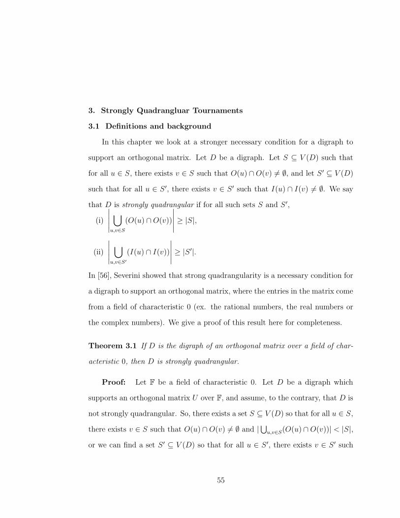
3. Strongly Quadrangluar Tournaments


In this chapter we look at a stronger necessary condition for a digraph to

support an orthogonal matrix. Let D be a digraph. Let S ⊆ V (D) such that

for all u ∈ S, there exists v ∈ S such that O(u) ∩ O(v) 6= ∅, and let S ′ ⊆ V (D)

such that for all u ∈ S ′, there exists v ∈ S ′ such that I(u) ∩ I(v) 6= ∅. We say

that D is strongly quadrangular if for all such sets S and S ′,

(i)

∣

∣

∣

∣

∣

⋃

u,v∈S

(O(u) ∩ O(v))

∣

∣

∣

∣

∣

≥ |S|,

(ii)

∣

∣

∣

∣

∣

⋃

u,v∈S′

(I(u) ∩ I(v))

∣

∣

∣

∣

∣

≥ |S ′|.

In [56], Severini showed that strong quadrangularity is a necessary condition for

a digraph to support an orthogonal matrix, where the entries in the matrix come

from a field of characteristic 0 (ex. the rational numbers, the real numbers or

the complex numbers). We give a proof of this result here for completeness.

Theorem 3.1 If D is the digraph of an orthogonal matrix over a field of char-

acteristic 0, then D is strongly quadrangular.

Proof: Let F be a field of characteristic 0. Let D be a digraph which

supports an orthogonal matrix U over F, and assume, to the contrary, that D is

not strongly quadrangular. So, there exists a set S ⊆ V (D) so that for all u ∈ S,

there exists v ∈ S such that O(u) ∩ O(v) 6= ∅ and |⋃u,v∈S(O(u) ∩ O(v))| < |S|,

or we can find a set S ′ ⊆ V (D) so that for all u ∈ S ′, there exists v ∈ S ′ such

55

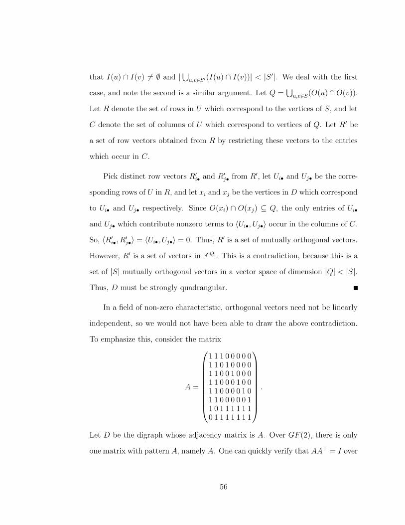
that I(u) ∩ I(v) 6= ∅ and |⋃u,v∈S′(I(u) ∩ I(v))| < |S ′|. We deal with the first

case, and note the second is a similar argument. Let Q =⋃

u,v∈S(O(u)∩ O(v)).

Let R denote the set of rows in U which correspond to the vertices of S, and let

C denote the set of columns of U which correspond to vertices of Q. Let R′ be

a set of row vectors obtained from R by restricting these vectors to the entries

which occur in C.

Pick distinct row vectors R′i• and R′

j• from R′, let Ui• and Uj• be the corre-

sponding rows of U in R, and let xi and xj be the vertices in D which correspond

to Ui• and Uj• respectively. Since O(xi) ∩ O(xj) ⊆ Q, the only entries of Ui•

and Uj• which contribute nonzero terms to 〈Ui•, Uj•〉 occur in the columns of C.

So, 〈R′i•, R

′j•〉 = 〈Ui•, Uj•〉 = 0. Thus, R′ is a set of mutually orthogonal vectors.

However, R′ is a set of vectors in F|Q|. This is a contradiction, because this is a

set of |S| mutually orthogonal vectors in a vector space of dimension |Q| < |S|.

Thus, D must be strongly quadrangular.

In a field of non-zero characteristic, orthogonal vectors need not be linearly

independent, so we would not have been able to draw the above contradiction.

To emphasize this, consider the matrix

A =

1 1 1 0 0 0 0 01 1 0 1 0 0 0 01 1 0 0 1 0 0 01 1 0 0 0 1 0 01 1 0 0 0 0 1 01 1 0 0 0 0 0 11 0 1 1 1 1 1 10 1 1 1 1 1 1 1

.

Let D be the digraph whose adjacency matrix is A. Over GF (2), there is only

one matrix with pattern A, namely A. One can quickly verify that AA> = I over

56

GF (2). If S ⊆ V (D) corresponding to the first 6 rows of A, then |⋃u,v∈S(O(u)∩

O(v))| = 2 < |S|, so D is not strongly quadrangular. So, strong quadrangularity

is only a necessary condition when dealing with fields of characteristic 0. For

this reason we will only deal with fields of characteristic 0 for the rest of the

chapter.

To see that strong quadrangularity is in fact a more restrictive condition,

consider the following tournament. Let T be a tournament with V (T ) =

{0, 1, 2, 3, 4, 5, 6, x, y} so that {0, 1, 2, 3, 4, 5, 6} induces the tournament QR7,

x → y and O(y) = I(x) = V (T ) − {x, y}. In section 2.5, we saw that T is

quadrangular. Now consider the set of vertices S = {0, 1, 5}. Since each of 0, 1, 5

beat x, we have that for all u ∈ S, there exits v ∈ S so that O(u) ∩ O(v) 6= ∅.

Also,∣

∣

∣

∣

∣

⋃

u,v∈S

(O(u) ∩ O(v))

∣

∣

∣

∣

∣

= |(O(0) ∩ O(1)) ∪ (O(0) ∩ O(5)) ∪ (O(1) ∩ O(5))|

= |{2, x} ∪ {2, x} ∪ {2, x}|

= 2

< |S|.

So T is not strongly quadrangular. We now construct a class of strongly quad-

rangular tournaments.

3.2 A class of strongly quadrangular tournaments

In this section we construct a class of strongly quadrangular tournaments.

The following lemma is a well known fact of tournaments. It is a corol-

lary to the fact that every n-tournament contains a transitive (blog2(n)c + 1)-

subtournament. We prove it here for completeness.

57

Lemma 3.2 Let T be a tournament on n ≥ 4 vertices. Then there must exist

distinct a, b ∈ V (T ) such that O(a) ∩ O(b) 6= ∅.

Proof: Pick a vertex a of maximum out-degree in T . As, n ≥ 4, d+(a) ≥ 2.

Pick a vertex b of maximum out-degree in the subtournament W induced on

O(a). As d+(a) ≥ 2, d+W (b) ≥ 1. Thus, |O(a) ∩ O(b)| = d+

W (b) ≥ 1.

Theorem 3.3 Pick l ≥ 1. Let T ′ be a strong tournament on the vertices

{1, 2, . . . , l}, and let T1, T2, . . . , Tl be regular or near-regular tournaments of or-

der k ≥ 5. Construct a tournament T on kl vertices as follows. Let V be a set

of kl vertices. Partition the vertices of V into l subsets V1, . . . , Vl of size k and

place arcs to form copies of T1, T2, . . . , Tl on V1, . . . , Vl respectively. Finally, add

arcs so that Vi ⇒ Vj if and only if i → j in T ′. Then the resulting tournament,

T , is a strongly quadrangular tournament.

Proof: Pick S ⊆ V (T ). Define the set

A = {Vi : ∃u 6= v ∈ S 3 u, v ∈ Vi},

and define the set

B = {Vi : ∃!u ∈ S 3 u ∈ Vi}.

Let α = |A|, and β = |B|. Then, since each Vi has k vertices, kα + β ≥ |S|.

Consider the subtournaments of T ′ induced on the vertices corresponding to A

and B. These are tournaments and so must contain a Hamiltonian path. So,

label the elements of A and B so that A1 ⇒ A2 ⇒ · · · ⇒ Aα and B1 ⇒ B2 ⇒

· · · ⇒ Bβ. By definition of A, each Ai contains at least two vertices of S, and

58

so if x, y ∈ S and x, y ∈ Ai, for i ≤ α − 1, then Ai+1 ⊆ O(x) ∩ O(y). Thus,∣

∣

∣

∣

∣

⋃

u,v∈S

O(u) ∩ O(v)

∣

∣

∣

∣

∣

≥ k(α − 1).

We now consider three cases depending on β.

First assume that β ≥ 2. Consider the vertices of S in B we see that if

x, y ∈ S and x ∈ Bi and y ∈ Bi+1 then O(y) ∩ Bi+1 ⊆ O(x) ∩ O(y). Thus,

|O(x) ∩ O(y)| ≥ k−12

, and so∣

∣

∣

∣

∣

⋃

u,v∈S

O(u) ∩ O(v)

∣

∣

∣

∣

∣

≥ k(α−1)+k − 1

2(β−1) ≥ k(α−1)+2β−2 ≥ k(α−1)+β.

Now, since T ′ is a tournament, either A1 ⇒ B1 or B1 ⇒ A1. If A1 ⇒ B1, then

for vertices x, y ∈ A1 we know B1 ⊆ O(x) ∩ O(y). Since no vertex of B1 had

been previously counted, we have that∣

∣

∣

∣

∣

⋃

u,v∈S

O(u) ∩ O(v)

∣

∣

∣

∣

∣

≥ k(α − 1) + β + k = kα + β ≥ |S|.

So, assume that B1 ⇒ A1. Then for the single vertex of S in B1, u, and a

vertex v of S in A1 O(v) ⊆ O(u)∩O(v). This adds k−12

vertices which were not

previously counted. Also, since T ′ is strong, some Ai ⇒ Vj for some Vj 6∈ A.

We counted at most k−12

vertices in Vj before, and since Ai contains at least

two vertices x, y from S these vertices add at least k+12

vertices which were not

previously counted, so∣

∣

∣

∣

∣

⋃

u,v∈S

O(u) ∩ O(v)

∣

∣

∣

∣

∣

≥ k(α − 1) + β +k − 1

2+

k + 1

2= kα + β ≥ |S|.

Now assume that β = 1. Since T ′ is strong we know that Ai ⇒ Vj for some

Vj 6∈ A. So,∣

∣

∣

∣

∣

⋃

u,v∈S

O(u) ∩ O(v)

∣

∣

∣

∣

∣

≥ kα.

59

Now, if |S| ≤ kα, then we are done, so assume that |S| = kα + 1. So, for every

Ai ∈ A, Ai ⊆ S. So by Lemma 3.2 we can find two vertices of S in A1 which

compete over a vertex of Ai, adding one more vertex to our count, and

∣

∣

∣

∣

∣

⋃

u,v∈S

O(u) ∩ O(v)

∣

∣

∣

∣

∣

≥ kα + 1 = |S|.

For the last case, assume that β = 0. Then since T ′ is strong we once again

have that some Ai ⇒ Vj for some Vj 6∈ A. Thus,

∣

∣

∣

∣

∣

⋃

u,v∈S

O(u) ∩ O(v)

∣

∣

∣

∣

∣

≥ kα ≥ |S|.

Note that the dual of T ′ will again be strong, and the dual of each Ti

will again be regular. Thus, by appealing to duality in T we have that for all

S ⊆ V (T ),∣

∣

∣

∣

∣

⋃

u,v∈S

I(u) ∩ I(v)

∣

∣

∣

∣

∣

≥ |S|,

and so T is a strongly quadrangular tournament.

Recall that strong quadrangularity is a necessary condition for a digraph

to support an orthogonal matrix. To emphasize that strong quadrangularity

is not sufficient, consider the strongly quadrangular tournament, T , which the

construction in the previous theorem gives on 15 vertices. For this tournament,

T1, T2 and T3 are all regular of order 5, and T ′ is the 3-cycle. Note that up

to isomorphism, there is only one regular tournament on 5 vertices, so without

loss of generality, assume that T1, T2 and T3 are the rotational tournament with

symbol {1, 2}. We now show that T cannot be the digraph of an orthogonal

matrix.

60

Recall J5 is the 5 × 5 matrix of all ones, and O5 the 5 × 5 matrix of all 0s.

Set

RT5 =

0 1 1 0 00 0 1 1 00 0 0 1 11 0 0 0 11 1 0 0 0

.

Then the adjacency matrix M of T is

M =

(

RT5 J5 O5

O5 RT5 J5

J5 O5 RT5

)

.

Now, suppose to the contrary that there exists an orthogonal matrix U whose

pattern is M . Observe from the pattern of U that the only entries of U which

contribute to 〈Ui, Uj〉 for i = 1, . . . , 5, j = 6, . . . , 10 are in the first five rows. So,

〈U1, Uj〉 = U4,1U4j + U5,1U5,j for j = 6, . . . , 10. Thus, since 0 = 〈U1, Uj〉 for each

j 6= 1,

U4,1 =−U5,1U5,6

U4,6=

−U5,1U5,7

U4,7=

−U5,1U5,8

U4,8=

−U5,1U5,9

U4,9=

−U5,1U5,10

U4,10.

Since U5,1 6= 0 this gives,

−U4,1

U5,1=

U5,6

U4,6=

U5,7

U4,7=

U5,8

U4,8=

U5,9

U4,9=

U5,10

U4,10.

So, the vectors (U4,6, . . . , U4,10) and (U5,6, . . . , U5,10) are scalar multiples of

each other. Now, note that for j = 6, . . . , 10, we have 0 = 〈U2, Uj〉 =

U1,2U1,j + U5,2U5,j. So, by applying the same argument, we see that the vec-

tor (U5,6, U5,7, U5,8, U5,9, U5,10) is a scalar multiple of (U1,6, U1,7, U1,8, U1,9, U1,10).

So, (U4,6, U4,7, U4,8, U4,9, U4,10) is a scalar multiple of (U1,6, U1,7, U1,8, U1,9, U1,10).

Now, from the pattern of U we see that only the 6th through 10th columns con-

tribute to 〈U1•, U4•〉. So, since linearly dependent vectors cannot be orthogonal,

〈U1•, U4•〉 = 〈(U1,6, U1,7, U1,8, U1,9, U1,10), (U4,6, U4,7, U4,8, U4,9, U4,10)〉 6= 0.

61

This contradicts our assumption that U is orthogonal. So, T is not the digraph

of an orthogonal matrix.

3.3 Nonexistence and searches

The only known tournament which supports an orthogonal matrix is the

3-cycle (This is a permutation matrix, and hence itself an orthogonal matrix).

Otherwise, the problem of determining whether or not there exist tournaments

which support orthogonal matrices has proved to be quite difficult. As we have

seen, for large values of n we can almost always construct examples of tourna-

ments which meet our necessary conditions. Knowing that almost all tourna-

ments are quadrangular and having a construction for an infinite class of strongly

quadrangular tournaments, one may believe that there will exist a tournament

which supports an orthogonal matrix. However, attempting to find an orthog-

onal matrix whose digraph is a given tournament has proved to be a difficult

task. In general, aside from the 3-cycle, the existence of a tournament which

supports an orthogonal matrix is still an open problem. The following result

may lead one to believe non-existence is the answer to this problem.

Theorem 3.4 Other than the 3-cycle, there does not exist a tournament on 10

or fewer vertices which is the digraph of an orthogonal matrix.

Proof: By Theorem 2.34 there exists a quadrangular n-tournament for

n ≤ 10 if and only if n is 1, 2, 3 or 9. Note, in the case n = 1 and n = 2,

the only tournaments are the single vertex and single arc, both of whose ad-

jacency matrices have a column of zeros. Since orthogonal matrices have full

rank, these cannot support an orthogonal matrix. When n = 3, the 3-cycle is

the only quadrangular tournament. The adjacency matrix for this tournament

62

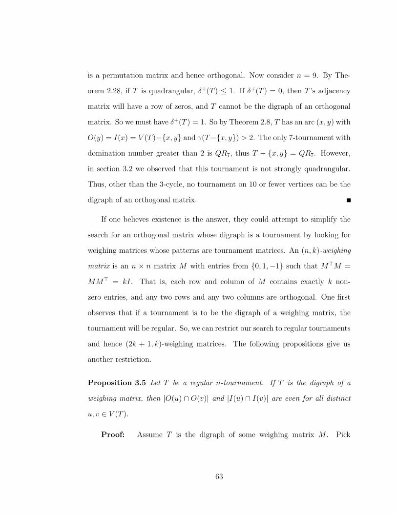
is a permutation matrix and hence orthogonal. Now consider n = 9. By The-

orem 2.28, if T is quadrangular, δ+(T ) ≤ 1. If δ+(T ) = 0, then T ’s adjacency

matrix will have a row of zeros, and T cannot be the digraph of an orthogonal

matrix. So we must have δ+(T ) = 1. So by Theorem 2.8, T has an arc (x, y) with

O(y) = I(x) = V (T )−{x, y} and γ(T−{x, y}) > 2. The only 7-tournament with

domination number greater than 2 is QR7, thus T − {x, y} = QR7. However,

in section 3.2 we observed that this tournament is not strongly quadrangular.

Thus, other than the 3-cycle, no tournament on 10 or fewer vertices can be the

digraph of an orthogonal matrix.

If one believes existence is the answer, they could attempt to simplify the

search for an orthogonal matrix whose digraph is a tournament by looking for

weighing matrices whose patterns are tournament matrices. An (n, k)-weighing

matrix is an n × n matrix M with entries from {0, 1,−1} such that M>M =

MM> = kI. That is, each row and column of M contains exactly k non-

zero entries, and any two rows and any two columns are orthogonal. One first

observes that if a tournament is to be the digraph of a weighing matrix, the

tournament will be regular. So, we can restrict our search to regular tournaments

and hence (2k + 1, k)-weighing matrices. The following propositions give us

another restriction.

Proposition 3.5 Let T be a regular n-tournament. If T is the digraph of a

weighing matrix, then |O(u) ∩ O(v)| and |I(u) ∩ I(v)| are even for all distinct

u, v ∈ V (T ).

Proof: Assume T is the digraph of some weighing matrix M . Pick

63

u, v ∈ V (T ) and let Mu•, Mv• be the rows of M which correspond to u and

v respectively. Note, 0 = 〈Mu•, Mv•〉 = Mu,1Mv,1 + Mu,2Mv,2 + · · · + Mu,nMv,n.

Now, Mu,iMv,i 6= 0 if and only if i ∈ O(u) ∩ O(v). Since 〈Mu•, Mv•〉 = 0, and

every non-zero term of∑n

i=1 Mu,iMv,i is ±1, we have that the number of nega-

tive terms in the sum must equal the number of positive terms. So, the number

of non-zero terms in the sum must be even. Hence, |O(u)∩O(v)| must be even.

Similarly, |I(u) ∩ I(v)| must be even.

Proposition 3.6 Let T be an n-tournament. If T is the digraph of a weighing

matrix, then n ≡ 1 or 3 (mod 8).

Proof: Assume that T is the digraph of some weighing matrix. Note, that

this implies T is a regular tournament. Now, choose u ∈ V (T ), and v ∈ O(u).

By Proposition 3.5, |O(u) ∩ O(v)| is even. Equivalently, d+T [O(u)](v) is even.

Since v was chosen from O(u) arbitrarily, d+T [O(u)](x) is even for all x ∈ O(u).

Thus,(

d+T

(u)2

)

=∑

x∈O(u) d+T [O(u)](x) must be even. So, 2|d

+T

(u)(d+T

(u)−1)

2, and so

4|d+T (u)(d+

T (u) − 1). Since d+T (u) and d+

T (u) − 1 must be relatively prime, we

have that 4|d+T (u) or 4|d+

T (u)−1. Since T is a regular tournament, d+T (u) = n−1

2.

So, 4|n−12

or 4|n−32

, and so 8|n − 1 or 8|n − 3. Hence n ≡ 1 or 3 (mod 8).

The following condition is well known for (n, k)-weighing matrices in which

n is odd. We prove it here for completeness.

Theorem 3.7 [27]If M is an (n, k) weighing matrix with n odd, then k is a

perfect square.

Proof: Let M be an (n, k)-weighing matrix, and assume n is odd. Then

det(M>M) = det(kI) = kn. Since, det(M>) = det(M) and det(M>M) =

64

det(M>) det(M), we have that det(M)2 = kn, and so det(M) = ±√

kn. Since n

is odd, n = 2b + 1 for some b, and so det(M) = ±kb√

k. Now, the determinant

of M is∑

σ∈SnM1,σ(1)M2,σ(2) · · ·Mn,σ(n) (where Sn denotes the symmetric group

of order n). So, since every entry of M is an integer, det(M) must be an integer

as well. Thus, kb√

k ∈ Z, and so√

k ∈ Z. That is, k is a perfect square.

Since a weighing matrix which has a tournament for its digraph will be a

(2k + 1, k)-weighing matrix, the previous theorem tells us we are looking for a

(2a2 + 1, a2)-weighing matrix. By examining cases, we get Proposition 3.6 as

the following corollary to Theorem 3.7.

Corollary 3.8 Let T be a regular n-tournament. If T is the digraph of a weigh-

ing matrix, then n ≡ 1 or 3 (mod 8).

Putting together the fact that we are looking for a (2a2 + 1, a2)-weighing

matrix with Theorem 3.4, we see that the smallest case we can start searching

for is a (19, 9)-weighing matrix. One obvious choice for a tournament to search

is QR19, since this is a regular 19 vertex tournament with the property that the

outsets of every two vertices intersect in exactly 4 vertices. With the aid of Carey

Jenkins, we constructed the following algorithm to search for a (19, 9)-weighing

matrix whose digraph is QR19. A tree diagram of the “branch and bound”

technique used in this algorithm is shown in Figure 3.1. In this diagram, circled

vertices represent the rows our algorithm has currently appended, and dashed

lines show paths which, by design of our algorithm, we need not search.

First construct and store all 29 = 512 possible assignments of −1 to the

65

R

R R

R

R

1,0

2,j2

3,j3

2,0 2,511

R4,j44

3

2

1

Rows

19

RR2,1 2,2

R

R R

18,j18

19,0 19,j19 19,511R

Figure 3.1: The tree diagram for our algorithm

non-zero entries of the first row of the adjacency matrix of QR19,

R1,0 = (0 1 0 0 1 1 1 1 0 1 0 1 0 0 0 0 1 1 0).

Label these as R1,j where j is a number between 0 and 511 which labels each

different assignment of −1s to the vector. Next, construct all cyclic shifts of

these rows. Label each row created in this way so that Ri,j is R1,j shifted i − 1

positions to the right. Since the adjacency matrix of QR19 is circulant, this

creates all possible assignments of −1 to the non-zero positions of row i, for

i = 2, . . . , 19.

We attempt to build a matrix by appending rows. We begin with the first

row R1,0 above. Lemma 3.9 shows why we can leave this row fixed. For j2 = 0,

66

compute 〈R1,0, R2,j2〉. If 〈R1,0, R2,j2〉 = 0, we append R2,j2 and move on to

find R3,j3 which is orthogonal to R1,0 and R2,j2 . If not, increment j2 and repeat.

Continue adding rows in this manner. Assume we have a matrix with i mutually

orthogonal rows,

R1,0

R2,j2...

Ri,ji

.

Set ji+1 = 0, and begin successively checking if Ri+1,ji+1is orthogonal to each

previously selected row, and incrementing ji+1 by 1 if not. If there is some

Ri+1,ji+1which is orthogonal to each of the previously selected rows, then ap-

pend it. If ji+1 reaches 512, and hence there does not exist a Ri+1,ji+1which is

orthogonal to each of the previous rows, then return to row i, increment ji, and

search for a new Ri,jiwhich is orthogonal to each of the previous i − 1 rows.

At each step the algorithm is maintaining a set of mutually orthogonal rows,

so if it finds 19 rows successfully, then it has created a (19, 9)-weighing matrix

whose digraph is QR19. Otherwise, for some k < 19, ji will reach 512 for all

2 ≤ i ≤ k, and we will have completely searched all possible combinations of

the first k rows without finding a set of k mutually orthogonal rows, and the

algorithm terminates showing no such matrix exists.

The C++ code for our implementation of this algorithm can be found in

appendix B. The algorithm was implemented in parallel on the University’s

Beowulf cluster. The search was split by giving the first 16 possible assignments

of row 2 to the first processor, the next 16 to the next processor, and so on.

After approximately 5 minutes, the algorithm terminated showing that QR19 is

not the digraph of a weighing matrix.

67

Lemma 3.9 Let M be an (n, k)-weighing matrix, and let M ′ be the matrix

obtained from M by multiplying any set of the rows of columns by −1. Then M ′

is an (n, k)-weighing matrix.

Proof: Let S ⊆ {1, . . . , n}, be the indices of the columns of M multiplied

by −1 to obtain M ′, and S ′ the indices of the rows multiplied by −1 to obtain

M ′. Let DS be the diagonal matrix whose i, i entry is −1 if i ∈ S and 1 if i 6∈ S.

Define DS′ to be the diagonal matrix whose i, i entry is −1 if i ∈ S ′ and 1 if

i 6∈ S ′. Note since (−1)(−1) = 1 ∗ 1 = 1, DS and DS′ are their own inverses.

Also, M ′ = DS′MDS. So,

M′>M ′ = (DS′MDS)>(DS′MDS)

= D>S M>D>

S′DS′MDS

= DSM>DS′DS′MDS

= DSM>IMDS

= DSM>MDS

= DS(kI)DS

= kDSIDs

= kDSDS

= kI,

and M ′ is an (n, k)-weighing matrix.

68

4. Fully Indecomposable Tournament Matrices


Another combinatorial necessary condition for a matrix to be orthogonal is

that it can be written in block form

A1 O O · · · OO A2 O · · · OO O A3 · · · O...

......

. . ....

O O O · · · Ak

where each Ai is fully indecomposable. This is a combinatorial property, so it is

also required of a (0, 1)-matrix to be the pattern of an orthogonal matrix. So,

in this chapter, we determine exactly which tournaments have adjacency matri-

ces which are fully indecomposable, and characterize the separable tournament

matrices.

Let A be an n × n matrix, n ≥ 2. Then A is called partly decomposable

provided there exist permutation matrices P and Q such that

PAQ =

(

B OD C

)

where O is an r × s matrix of zeros with r + s = n, and B and C are square

matrices other than the zero matrix. If A cannot be permuted into this form,

then we say that A is fully indecomposable. If A has a row or column of zeros,

or we can independently permute the rows and columns of A so that

A =

(

B OO C

)

69

then we say that A is separable. This property has also been called totally

decomposable, by Brualdi, Harary and Miller, [11], and disconnected by Green-

berg, Lundgren, and Maybee, [29]. If a matrix is not separable, we say it is

inseparable.

If we require simultaneous row and column permutations, then we say a

matrix which can be permuted into the form

(

B OD C

)

is reducible, and irreducible

otherwise. If M is the adjacency matrix of a digraph D, it is a well known

result that M is irreducible if and only if D is strongly connected. However,

as mentioned in chapter 1, independent row and column permutations do not

necessarily result in the same digraph. So, it is difficult to determine just what

these properties mean in digraphs.

Since independent row and column permutations do not necessarily result

in isomorphic digraphs, when looking at a matrix property that allows for inde-

pendent row and column permutations, one typically wants to treat the matrix

as a reduced adjacency matrix of a bipartite graph. Given a bipartite graph

B with bipartition X = {x1, . . . , xm} and Y = {y1, . . . , yn}, the reduced adja-

cency matrix of B is the m × n (0, 1)-matrix M with Mi,j = 1 if and only if

[xi, yj] ∈ E(B). By treating a (0, 1)-matrix as the reduced adjacency matrix of

a bipartite graph, independent row and column permutations will result in the

reduced adjacency matrix of an isomorphic bipartite graph. For instance, con-

sider the following matrix M . By exchanging the 5th and 7th rows, and swapping

70

the 1st and 3rd and the 2nd and 5th columns we obtain the matrix M ′.

M =

0 1 0 0 0 0 00 0 0 1 0 0 01 0 0 0 0 0 00 0 1 0 1 1 00 0 0 0 0 0 10 0 0 0 1 0 00 0 0 0 0 1 0

M ′ =

0 0 0 0 1 0 00 0 0 1 0 0 00 0 1 0 0 0 01 1 0 0 0 1 00 0 0 0 0 1 00 1 0 0 0 0 00 0 0 0 0 0 1

Both M and M ′ represent the same bipartite graph B shown in Figure 4.1. How-

ever, M and M ′ represent the digraphs D and D′ respectively from Figure 4.2,

and clearly D and D′ are not isomorphic.

Figure 4.1: A bigraph representation of M and M ′

Despite this problem, we are interested in characterizing tournaments with

properties which require independent row and column permutations. So, we

study how these properties affect digraphs, and in particular, tournaments. For

fully indecomposable digraphs, we look at the matrix before the permutations,

and for separable matrices we look at competition graphs.

We obtain our characterization of separable tournament matrices by utiliz-

ing the characterization of the competition graphs of tournaments via the char-

acterization of the domination graphs of tournaments. We will also use these

71

D D’

Figure 4.2: Different digraph representations for M and M ′.

characterizations to obtain some interesting corollaries about tournaments and

tournament matrices. We see exactly when a tournament matrix has a mini-

mum line cover other than the all rows or all columns cover. We characterize the

tournaments which are the digraphs of doubly-stochastic matrices, and give a

necessary condition for a tournament to be the digraph of an orthogonal matrix.

We also characterize the tournaments for which every arc is contained in a cycle

factor.

4.2 Fully indecomposable matrices

Let M be the adjacency matrix of a digraph D, and suppose M is partly

decomposable. So we can perform independent row and column permutations

to create an r × s block of zeros in M with r + s = n. By permuting the rows

and columns of M back to their original positions, we see that the block of

zeros corresponds to two sets of vertices X and Y , not necessarily disjoint, with

|X| = r and |Y | = s, and there is no arc (x, y) with x ∈ X and y ∈ Y . We

72

use this interpretation of the partly decomposable property to get the following

theorem.

Theorem 4.1 Let T be a tournament on n vertices, and let M be its adjacency

matrix. Then M is fully indecomposable if and only if T is strongly connected

and does not contain a vertex v such that T − v contains a strong component of

order 1.

Proof: Suppose M is partly decomposable. So there exist sets X, Y ⊆

V (T ) so that there is no arc of T from X to Y , and |X| + |Y | = n. Suppose

that |X ∩ Y | ≥ 2. Then there exist distinct vertices u, v ∈ X ∩ Y . Since T is a

tournament either u → v or v → u. Without loss of generality say u → v. This

cannot be since u ∈ X and v ∈ Y . Therefore |X ∩ Y | ≤ 1. We now consider

two cases based on |X ∩ Y |.

Case 1: Suppose |X ∩ Y | = 0. Then since |X| + |Y | = n, X and Y form a

partition of the vertices of T . Thus, since X and Y partition V (T ) and no

vertex in X beats any vertex in Y , T is not strongly connected.

Case 2: Suppose |X ∩ Y | = 1. So X ∩ Y = {u} and X ∪ Y = V (T ) − {v} for

some u 6= v ∈ V (T ). Further, since u ∈ Y , u ⇒ X − {u} and since u ∈ X,

Y − {u} ⇒ u. Finally, since no vertex in X beats any vertex in Y , we have

Y ⇒ X − {u}. Thus, T − v contains a strong component of order 1, namely u.

For the converse, recall that if a tournament is not strongly connected, it can

be partitioned into m ≥ 2 strong components T1, T2, . . . , Tm such that Ti ⇒ Tj if

and only if i < j. So, if T is not strongly connected, then taking X = V (Tm) and

Y = V (T1)∪V (T2)∪· · ·∪V (Tm−1) gives X and Y so that |X|+|Y | = n and there

73

is no arc from X to Y . Now, suppose T contains a vertex v so that T ′ = T − v

is not strongly connected and has a strong component, say T ′i , of order 1. Then

take X = V (T ′i ) ∪ V (T ′

i+1) ∪ · · · ∪ V (T ′m) and Y = V (T ′

1) ∪ V (T ′2) ∪ · · · ∪ V (T ′

i ).

Then |X| + |Y | = n and there is no arc from X to Y .

4.3 Separable matrices

Let M be an n × n (0, 1)-matrix, and let B be a bipartite graph who’s

reduced adjacency matrix is M , and D a digraph who’s adjacency matrix is

M . Then one can quickly verify that M being inseparable is equivalent to B

being connected. Unfortunately, there is no direct connection between M being

inseparable and a connectedness property of D. However, in [29], Greenberg,

Lundgren and Maybee showed that there is a connection between M being

inseparable and connectedness in two more graphs other than B. The row graph

of M is the graph whose vertices correspond to the rows of M , with vertices

i and j adjacent if and only if there exists some k so that Mi,k = Mj,k = 1.

Similarly, the column graph of M is the graph whose vertices correspond to the

columns of M , with vertices i and j adjacent if and only if there exists some k

so that Mk,i = Mk,j = 1. We now state their result.

Theorem 4.2 [29] Let M be an m × n matrix such that each column and row

of M has a non-zero element. Then the following are equivalent.

1) The bipartite graph whose reduced adjacency matrix is M is connected.

2) The row graph of M is connected.

3) The column graph of M is connected.

74

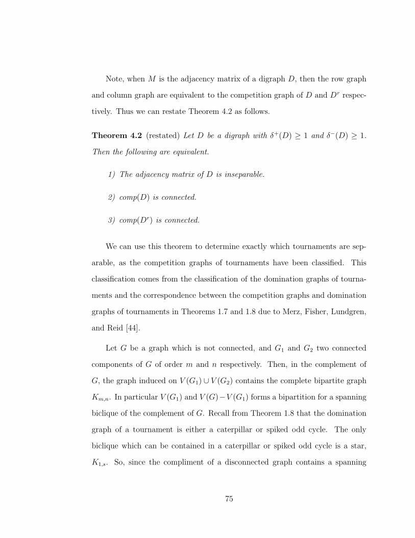
Note, when M is the adjacency matrix of a digraph D, then the row graph

and column graph are equivalent to the competition graph of D and Dr respec-

tively. Thus we can restate Theorem 4.2 as follows.

Theorem 4.2 (restated) Let D be a digraph with δ+(D) ≥ 1 and δ−(D) ≥ 1.

Then the following are equivalent.

1) The adjacency matrix of D is inseparable.

2) comp(D) is connected.

3) comp(Dr) is connected.

We can use this theorem to determine exactly which tournaments are sep-

arable, as the competition graphs of tournaments have been classified. This

classification comes from the classification of the domination graphs of tourna-

ments and the correspondence between the competition graphs and domination

graphs of tournaments in Theorems 1.7 and 1.8 due to Merz, Fisher, Lundgren,

and Reid [44].

Let G be a graph which is not connected, and G1 and G2 two connected

components of G of order m and n respectively. Then, in the complement of

G, the graph induced on V (G1) ∪ V (G2) contains the complete bipartite graph

Km,n. In particular V (G1) and V (G)−V (G1) forms a bipartition for a spanning

biclique of the complement of G. Recall from Theorem 1.8 that the domination

graph of a tournament is either a caterpillar or spiked odd cycle. The only

biclique which can be contained in a caterpillar or spiked odd cycle is a star,

K1,s. So, since the compliment of a disconnected graph contains a spanning

75

biclique, Theorems 4.2, 1.7 and 1.8 tell us that a tournament on n vertices with

no transmitter or receiver has a separable adjacency matrix, if and only if its

dual has a domination graph which contains the star K1,n−1.

Lemma 4.3 Let T be an n-tournament. Then dom(T ) contains K1,n−1 as a

subgraph, if and only if T has a transmitter, or T contains an arc (x, y) so that

O(y) = I(x) = V (T ) − {x, y}.

Proof: Suppose the star K1,n−1 is a subgraph of dom(T ), and let y be

the center of K1,n−1. Suppose there exist distinct u, v ∈ V (T ) such that u → y

and v → y, and without loss of generality, suppose u → v. Then neither y

nor v dominate u, however [y, v] is an edge in dom(T ), a contradiction. Thus,

d+(y) ≥ n − 2. If d+(y) = n − 1, then y is a transmitter and we are done. So

assume d+(y) = n− 2 and hence d−(y) = 1. Let x be the unique vertex in I(y).

Now choose u ∈ V (T ) − {x, y}. Since I(y) = {x}, we have y → u. Also, since

[y, u] is an edge in dom(T ), and x → y we must have u → x. Thus, there exists

an arc (x, y) in T with O(y) = I(x) = V (T ) − {x, y}. So these conditions are

necessary.

For sufficiency, first suppose T has a transmitter s. Pick a vertex v other

than s in V (T ). If u ∈ V (T ) − {s, v} then s → u, so [s, v] ∈ E(dom(T )). Since

v was chosen arbitrarily, the star K1,n−1 is a subgraph of dom(T ) with center s.

Now, assume T contains and arc (x, y) so that O(y) = I(x) = V (T ) − {x, y}.

Choose w ∈ V (T )−{x, y}. If z ∈ V (T )−{x, y, w}, then y → z, and w → x. So,

[y, w] ∈ E(dom(T )) for each w ∈ V (T ) − {x, y}. Further, [x, y] ∈ E(dom(T ))

since y → z for all z ∈ V (T ) − {x, y}. So dom(T ) contains the star K1,n−1 as a

76

subgraph with center y.

By Lemma 4.3 and Theorems 4.2 and 1.7, if T is a tournament with no

transmitter or receiver, T ’s adjacency matrix is separable if and only if T r con-

tains an arc (x, y) with O(y) = I(x) = V (T ) − {x, y}. Note however, if T r

contains such an arc so will T . Also, if T has a transmitter or receiver its adja-

cency matrix has a row or column of zeros, and is separable. This gives us the

following theorem.

Theorem 4.4 Let T be a tournament. Then the adjacency matrix of T is sep-

arable if and only if at least one of the following occur.

1. T has a transmitter.

2. T has a receiver.

3. There exists an arc (x, y) in T such that O(y) = I(x) = V (T ) − {x, y}.

4.4 Corollaries

In this section we give some corollaries due to our characterizations and

previous results about fully indecomposable matrices. Our first result involves

line covers of tournament matrices. A line cover of a matrix, M , is a set of

rows and columns of M which contain every non-zero entry of M . The following

theorem is taken from [14].

Theorem 4.5 A matrix M has a minimum line cover other than the all rows

or all columns cover if and only if M is partly decomposable.

77

The size of a minimum line cover is called the term rank of a matrix. In

Chapter 6 we will see that an n × n tournament matrix can only have real

rank, and hence term rank, n or n − 1. In [22], Doherty, Lundgren and Siewert

show that the tournaments whose adjacency matrices have term rank n− 1 are

exactly those with a strong component of order 1. The following corollary shows

that not only is the class of tournament matrices with term rank n − 1 highly

restricted, the class of tournaments whose adjacency matrices admit a minimum

line cover other than the all rows or all columns cover is fairly restricted.

Corollary 4.6 Let T be a tournament and M its adjacency matrix. Then M

has a minimum line cover other than the all rows or all columns cover if and

only if T is not strongly connected, or T contains a vertex v such that T − v has

a strong component of order 1.

Our remaining results are concerned with when a matrix has the property

that each of its inseparable components is fully indecomposable. Note, when a

matrix contains a row or column of zeros, one of the inseparable components

will be a submatrix of zeros and, hence, not fully indecomposable. So, in the

following theorem, we may assume that our tournaments have no transmitters

or receivers.

Theorem 4.7 Let T be a tournament with δ+(T ) ≥ 1, δ−(T ) ≥ 1, and adja-

cency matrix M . Then each inseparable component of M is fully indecomposable

if and only if

1. T is strongly connected, and

78

2. if T contains a vertex v such that T −v has a strong component of order

1, then T contains an arc (x, y) with O(y) = I(x) = V (T ) − {x, y} and

T − {x, y} does not contain a strong component of order 1.

Proof: If T is not strongly connected, then by Theorem 4.1, M must be

partly decomposable. Further, in this case the only way M could be separable

is for T to have a transmitter or receiver, a contradiction to our assumption

that δ+(T ) ≥ 1 and δ−(T ) ≥ 1. Thus 1. is necessary, and we may assume T is

strongly connected. If M is fully indecomposable we are done, so assume M is

partly decomposable. By Theorem 4.1, M is partly decomposable if and only

if T contains a vertex v such that T − v has a strong component of order 1.

Suppose M is separable. Since T has no transmitter or receiver, Theorem 4.4

says T must have an arc (x, y) such that O(y) = I(x) = V (T ) − {x, y}. Now,

consider the submatrix of M obtained by deleting the row and column of M

corresponding to O(x) and I(y) respectively. This matrix has the form

A =

[

1 11 M ′

]

where M ′ is an (n − 2) × (n − 2) tournament matrix and 1 denotes a vector of

all ones. Let T ′ be a tournament with adjacency matrix M ′. Note, A is partly

decomposable if and only if there exist sets X, Y ⊆ V (T ′) with no arc from X

to Y , and |X|+ |Y | = n − 1. Now, |X ∪ Y | ≤ |V (T ′)| = n − 2 and since T ′ is a

tournament, |X ∩ Y | ≤ 1. So,

n − 1 = |X| + |Y | = |X ∪ Y | + |X ∩ Y | ≤ n − 2 + 1 = n − 1.

Thus, |X ∪Y | = n−2 = |V (T ′)| and |X ∩Y | = 1, which occurs exactly when T ′

has a strong component of order 1. Further, since A contains a row and column

79

of all ones, A cannot be separable. Thus, each inseparable component of M is

fully indecomposable if and only if T is strongly connected and if T contains a

vertex v such that T − v has a strong component of order one, then T contains

a arc (x, y) such that O(y) = I(x) = V (T ) − {x, y} and T − {x, y} does not

contain a strong component of order 1.

In our next two results we look at when tournaments are the digraphs of

doubly-stochastic and orthogonal matrices. A real non-negative n× n matrix is

called doubly-stochastic if every row sum and column sum is 1. The following

theorem is taken from [14].

Theorem 4.8 A (0, 1)-matrix M is the pattern of a doubly-stochastic matrix if

and only if every inseparable component of M is a fully indecomposable matrix.

This theorem together with Theorem 4.7 give us the following corollary.

Corollary 4.9 A tournament T is the digraph of a doubly-stochastic matrix if

and only if,





The following theorem is taken from the linear algebra folklore. We prove

it here for completeness.

80

Theorem 4.10 If M is an orthogonal matrix, then each inseparable component

of M is a fully indecomposable matrix.

Proof: Let M be an n × n orthogonal matrix. Note if M is separable,

then M can be written in the form

A1 O O · · · OO A2 O · · · OO O A3 · · · O...

......

. . ....

O O O · · · Ak

where each Ai is inseparable. Block multiplication shows that if M is orthogonal

each Ai must also be orthogonal. So, we may assume M is inseparable. Now,

suppose to the contrary that M is partly decomposable. Say M can be written

in the form

M =

(

A OB C

)

where O is a p × q matrix of 0s with p + q = n. Then,

In =

(

Ip OO Iq

)

=

(

A OB C

)(

A> B>

O> C>

)

=

(

AA> AB>

BA> (BB> + CC>)

)

.

So, AA> = Ip, and since A is a square matrix, A is invertible. Then since

AB> = O, AB>i• = 0 for all i = 1, . . . q, a contradiction to A being invertible.

Thus, M cannot be partly decomposable and is hence fully indecomposable.

Again, using Theorem 4.7 we get the following corollary.

Corollary 4.11 If a tournament T is the digraph of an orthogonal matrix, then,


81




Note, unlike the previous two corollaries, this did not give us a character-

ization. This result only gives a necessary condition. Recall, as mentioned in

Chapter 3, aside from the 3-cycle, it is unknown if a tournament can be the

digraph of an orthogonal matrix.

Our final corollary is graph theoretic. A cycle factor of a digraph D is a

spanning subdigraph of D composed of vertex disjoint cycles. For example, the

bold arcs form a cycle factor of the digraph in Figure 4.3.

Figure 4.3: An example of a cycle factor in a digraph.

A non-zero diagonal of an n×n matrix M is a set of n non-zero elements of M

no two of which occur in the same row or column. If M is the adjacency matrix

of a digraph D, then the cycle factors of D are in direct correspondence with

non-zero diagonals of M . For example, the following matrix is the adjacency

82

matrix of the digraph in Figure 4.3. The bold ones in this matrix form a non-zero

diagonal and correspond to the bold arcs in the cycle factor in Figure 4.3.

0 1 0 1 1 00 0 1 0 1 11 0 0 1 0 10 1 0 0 1 00 0 1 0 0 11 0 0 1 0 0

The following theorem is taken from [14].

Theorem 4.12 Let M be an n × n (0, 1)-matrix. Then every 1 of M is on a

non-zero diagonal of M if and only if each inseparable component of M is fully

indecomposable.

This theorem together with Theorem 4.7, and the correspondence between

non-zero diagonals and cycle factors give us the following corollary.

Corollary 4.13 Let T be a tournament. Then every arc of T is contained in a

cycle factor if and only if,



1, then T contains an arc x → y with O(y) = I(x) = V (T ) − {x, y} and


83

5. Domination Graphs of Complete Paired Comparison Digraphs


In Chapter 4 we observed how a classification of the domination graphs

of tournaments gave us quite a bit of information about tournament matrices.

A generalized tournament matrix is a non-negative matrix M so that Mi,j +

Mj,i = 1 for all i 6= j, and Mi,i = 0 for all i. In this chapter we characterize

the domination graphs of the digraphs associated with generalized tournament

matrices, which we call complete paired comparison digraphs. A complete paired

comparison digraph, D, is a complete symmetric directed graph so that for each

arc (x, y) we associate a real number between 0 and 1, denoted wxy, such that

wyx = 1−wxy. We also refer to a complete paired comparison digraph as a pcd,

rather than the awkward cpcd.

Like the round robin competition model for tournaments, we can think

of a pcd as a model in which each vertex competes with all others, where if

x, y ∈ V (D), wxy denotes the probability that x will beat y. Based on this we

define a concept of domination in pcds. If D is a pcd, and x, y, z ∈ V (D) we

say that x and y dominate z if wxz + wyz ≥ 1. This is analogous to a dominant

pair in a tournament, when we ask the question as to which pairs of vertices

{x, y} dominate D. We say that vertices x and y form a dominant pair in a

complete paired comparison digraph D if for all z ∈ V (D) − {x, y} we have

wxz + wyz ≥ 1. A tournament can be considered a pcd with arc weights 0 or 1.

84

So, a dominant pair in a tournament is also a dominant pair in the tournament

when it is treated as a pcd.

If D is a pcd, then we define the domination graph of D, denoted dom(D),

on the same vertices of D with [x, y] an edge of dom(D) if and only if {x, y}

is a dominant pair. By studying the domination graphs of pcds, we can get a

feel for who a dominant competitor may be in the model. In [51] Moon and

Pullman also attempt to rank competitors in this model using the eigenvalues

of generalized tournaments.

Surprisingly, there is a distinction between domination graphs of pcds in

which some competitors are equally matched (i.e., the arcs between them have

weight .5) and domination graphs of pcds having no equally matched competi-

tors. We characterize domination graphs of pcds in which wxy 6= .5 for all

x, y ∈ D. We also characterize domination graphs of pcds in which the domina-

tion graphs are connected graphs, and in which the domination graphs have no

isolated vertices.

5.2 Preliminary results

In this section we give some preliminary results that will be used throughout

the chapter. A key to this study is the following lemma.

Lemma 5.1 Let D be a complete paired comparison digraph. For any 2 vertex

disjoint edges in dom(D), say [r, s] and [u, v], we have that in D

wru = wus = wsv = wvr.

Proof: Since {r, s} and {u, v} are dominant pairs in D, we know that

wvr + wur ≥ 1, wrv + wsv ≥ 1, wsu + wru ≥ 1, and wvs + wus ≥ 1. Also, by

85

the definition of a pcd, wru + wur = 1, wus + wsu = 1, wsv + wvs = 1, and

wvr + wrv = 1. Thus,

wru = 1 − wur ≤ wvr = 1 − wrv ≤ wsv = 1 − wvs ≤ wus = 1 − wsu ≤ wru,

and so

wru = wus = wsv = wvr.

Recall Un is the rotational tournament on the vertices {0, 1, 2 . . . , n − 1}

with i → j if and only if j − i is odd modulo n. In [44], Merz et. al. show that

Un is the unique tournament which has an n-cycle as its domination graph. We

now prove a similar result for an analogous pcd. Choose 0 ≤ p ≤ 1. We define

the pcd Un,p on vertex set {1, 2, . . . , n} by wij = p if and only if j − i is odd

modulo n, and wij = 1 − p otherwise.

Lemma 5.2 If n is odd, and Cn is an induced subgraph of the domination graph

of some complete paired comparison digraph D, then the vertices which induce

the cycle in dom(D) induce Un,p in D, for some p, 0 ≤ p ≤ 1.

Proof: We assume V (Cn) = {1, 2, . . . , n} and E(Cn) = {[i, i + 1] : 1 ≤ i ≤

n − 1} ∪ {[n, 1]}. Suppose that n ≥ 5. Consider the arc (1, j), 2 ≤ j ≤ n − 2.

Assume that j − 1 is odd. Let w1j = p. Apply Lemma 5.1 to edges [n, 1] and

[j, j + 1] to see that w1j = wjn = wn(j+1) = w(j+1)1 = p. Apply Lemma 5.1 to

edges [1, 2] and [j + 1, j + 2] to see that w(j+2)1 = w1(j+1) = 1− w(j+1)1 = 1− p.

Thus, w1(j+2) = p, and w1(j+1) = 1− p. This implies that all arc weights w1j are

p when j − 1 is odd and 1 − p when j − 1 is even, 2 ≤ j ≤ n. By an identical

86

argument with i in place of 1, if wij = q for j− i odd, then all arc weights wij are

q when j− i is odd and 1−q when j− i is even. Thus, p = w12 = 1−w21 = 1−q.

So, p + q = 1. Consequently, in D, wij = p if and only if j − i is odd modulo n,

and wij = 1 − p otherwise. Thus, V (Cn) induces Un,p in D.

To complete the proof, suppose that n = 3. Then, since {1, 3}, {1, 2} and

{2, 3} form dominant pairs, w12 + w32 ≥ 1, w13 + w23 ≥ 1, and w21 + w31 ≥ 1.

This means that w12+(1−w23) ≥ 1, w23+(1−w31) ≥ 1, and w31+(1−w12) ≥ 1.

Thus,

w12 ≥ w23 ≥ w31 ≥ w12.

So, the result follows.

Lemma 5.3 Let D be a complete paired comparison digraph with at least 4

vertices. Then, dom(D) = Kn if and only if wxy = .5 for all distinct x, y ∈

V (D).

Proof: Suppose dom(D) = Kn, and pick distinct x, y ∈ V (D). As n ≥ 4,

there are vertex disjoint edges [x, x′] and [y, y′] in dom(D). By Lemma 5.1,

wxy = wyx′ = wx′y′ = wy′x. Now, apply Lemma 5.1 to edges [x, y′] and [x′y]

to see that wyx = wxx′ = wx′y′ = wy′y. Therefore, wxy = wx′y′ = wyx. But

wyx = 1 − wxy, so wxy = wyx = .5, as desired. The converse is immediate.

Note, it was shown in Lemma 5.2 that if D is a pcd with 3 vertices x, y, z so

that wxy = wyz = wzx > .5, then dom(D) = K3. So, sufficiency of Lemma 5.3

requires our pcd have 4 or more vertices.

Theorem 5.4 Let D be a complete paired comparison digraph, and S ⊆ V (D).

87

Let D′ be the pcd induced on S, then the subgraph of dom(D) induced on S is a

subgraph of dom(D′).

Proof: Let {x, y} be a dominant pair in D, with x, y ∈ S. Then, for all

v ∈ V (D)− {x, y}, wxv + wyv ≥ 1. In particular, this is true of all v ∈ S. Thus,

{x, y} form a dominant pair in D′. This proves our result.

If D is a pcd, v ∈ V (D), and S ⊆ V (D), then we define the set O+S (v) by

O+S (v) = {x ∈ S : wvx > .5}.

If S = V (D), then O+V (D)(v) will be abbreviated as O+(v).

Lemma 5.5 Let D be a complete paired comparison digraph, v ∈ V (D), and

S ⊆ V (D). Then, O+S (v) forms an independent set in dom(D).

Proof: Let x, y ∈ O+S (v). Then, wxv < .5, and wyv < .5, so wxv + wyv < 1.

That is, {x, y} does not form a dominant pair.

Lemma 5.6 Let D be a pcd. There exists a pcd D′ on the same vertices as D

such that dom(D′) =dom(D), wxy < 1 for all x, y ∈ V (D′), and wxy is greater

than, less than, or equal to .5 in D′ if and only if it is greater than, less than,

or equal to .5 in D respectively.

Proof: If wxy < 1 for all x, y ∈ V (D), we are done. So, assume wxy = 1

for some x, y ∈ V (D). Let k = min{|wuv − .5| : u, v ∈ V (D), wuv 6= .5}, and

set ε = k2. For simplicity, for the rest of this proof we will let w′

xy denote the

weight of arc (x, y) in D′ and wxy the weight of arc (x, y) in D. We construct

D′ by setting V (D′) = V (D), and for distinct u, v ∈ V (D′) assigning weights

88

to (u, v) as follows. If wuv = .5, set w′uv = .5. If wuv > .5, set w′

uv = wuv − ε,

and if wuv < .5, set w′uv = wuv + ε. So, w′

xy < 1 for all x, y ∈ V (D′), and w′xy

is less than, greater than, or equal to .5 if and only if wxy is. We now show

dom(D′) =dom(D).

Pick [x, y] ∈ E(dom(D)). So, for all z ∈ V (D), wxz + wyz ≥ 1. Choose

z ∈ V (D). If wxz = wyz = .5, then w′xz + w′

yz = .5 + .5 = 1. If exactly one

of wxy and wyz is .5, then the other must be strictly greater than .5 or else

wxz + wyz < .5 + .5 = 1. So, w′xz + w′

yz = wxz + wyz − ε. By our choice of ε,

ε < wxz + wyz − 1, so w′xz + w′

yz ≥ 1. So, assume wxz and wyz are not .5. By a

similar argument, at least one of wxz and wyz must be strictly greater than .5.

So,

w′xz + w′

yz =

{

wxz + ε + wyz − ε, if wxz > .5, wyz < .5,wxz − ε + wyz + ε, if wxz < .5, wyz > .5,wxz + ε + wyz + ε, if wxz > .5, wyz > .5.

In all three cases, w′xz +w′

yz ≥ 1 since wxz +wyz ≥ 1. Thus, [x, y] ∈ E(dom(D′))

Now choose distinct x, y ∈ V (D′) so that [x, y] 6∈ E(dom(D)). So, for some

z ∈ V (D), wxz + wyz < 1. So either wxz < .5 or wyz < .5, or else wxz + wyz ≥ 1.

So,

w′xz + w′

yz =

wxz + wyz + ε, if wxz = .5, wyz < .5,wxz + ε + wyz, if wxz < .5, wyz = .5,wxz + ε + wyz − ε, if wxz > .5, wyz < .5,wxz − ε + wyz + ε, if wxz < .5, wyz > .5,wxz − ε + wyz − ε, if wxz < .5, wyz < .5.

In the first two cases, our choice of epsilon gives ε < 1 − (wxz + wyz), and

so wxz + wyz + ε < 1. In the last three cases, we have w′xz + w′

yz < 1, since

wxz + wyz < 1, and so [x, y] 6∈ E(dom(D)). Thus dom(D) =dom(D′).

The next proposition indicates why a characterization of domination graphs

of pcds is difficult. Consider the situation for tournaments. There are strict

89

requirements on a graph G so that there exist a tournament T for which dom(T )

contains G as an induced subgraph. This is not so in the context of pcds since

any graph will do as seen in the next proposition.

Proposition 5.7 Let G be a graph, then there exists a complete paired compar-

ison digraph D for which dom(D) contains G as an induced subgraph.

Proof: Let G be a graph on n vertices, and construct a pcd D in the

following way. Start with V (D) = V (G). For each x, y ∈ V (G), let wxy = .5.

Now, for each pair {i, j} of nonadjacent distinct vertices in G, add a vertex vij

(same as vji) to V (D), and set wvij i = wvijj = 1. Also, for each z ∈ V (G) with

[i, z] ∈ E(G) or [j, z] ∈ E(G), set wzvij= 1. Set all other weights to .5. We now

show the construction gives the desired result.

Consider two vertices x, y ∈ V (G). Suppose that [x, y] ∈ E(G). If [x, y] 6∈

dom(D), then there is a z ∈ V (D) so that wxz + wyz < 1. Because arc weights

are 0, .5, or 1, this implies that at least one of wxz or wyz is 0. Suppose wxz = 0;

then by construction z = vxk for some vertex k. But, since [x, y] ∈ E(G), the

construction yields wyz = 1. So, wxz + wyz = 1, a contradiction. Hence [x, y] is

in dom(D).

On the other hand, if [x, y] 6∈ E(G), then using z = vxy we see that wxz +

wyz = 0 + 0 = 0 so that {x, y} is not a dominating pair in D. That is, [x, y] 6∈

E(dom(D)). So, G is an induced subgraph of dom(D).

5.3 Complete paired comparison digraphs with no arc weight .5

As Proposition 5.7 shows, characterizing the domination graphs of pcds is

not an easy task. However, the problems seem to arise from equally matched

90

competitors. So, in this section, we will assume that wxy 6= .5 for every arc (x, y)

in our pcd. This is not such a bad assumption for it is rare that two competitors

are truly evenly matched. This assumption also gives a strong relation between

tournaments and pcds, as we shall see.

Let D be a pcd with no arc weight equal to .5. With D we associate a

digraph T defined on the same vertices of D, where x → y in T if wxy > .5.

So for all x, y ∈ V (T ), we have exactly one of x → y or y → x, i.e. T is a

tournament. We refer to T as D’s associated tournament.

Lemma 5.8 Let D be a complete paired comparison digraph with no weight

equal to .5, and T the associated tournament. Then dom(D) is a subgraph of

dom(T ). Furthermore, if D has only two weights, a > .5, and 1 − a, then

dom(D) =dom(T ).

Proof: Let {x, y} be a dominant pair in D. Then for each v ∈ V (D) −

{x, y}, wxv + wyv ≥ 1. So, since wxv 6= .5 and wyv 6= .5, either wxv > .5 or

wyv > .5. This implies that either x → v or y → v in T . Thus, {x, y} is a

dominant pair in T . So, dom(D) is a subgraph of dom(T ).

Now, suppose that D has only two weights, a > .5 and 1 − a. Let {x, y}

be a dominant pair in T . That is, for any other vertex v, x → v or y → v,

i.e. wxv > .5 or wyv > .5. As a > .5, this implies that wxv = a > 1 − a or

wyv = a > 1 − a, so wxv + wyv ≥ a + (1 − a) = 1. This means that {x, y} is a

dominant pair in D. Consequently, dom(D) = dom(T ).

We point out that if the pcd D has more than two weights, we may have

proper containment in the previous lemma. For instance, consider the pcd D

91

in Figure 5.1. Shown next to D is its associated tournament T . As shown in

Figure 5.2, dom(T ) is a spiked 3-cycle, while dom(D) is only a 2-path.

1 2

34

1 2

34

.7

.6 .7

.3

.3

.3

.7

.7.3

.6

.4

.4

D T

Figure 5.1: A pcd and its associated tournament

Recall from Theorem 1.8, that the domination graph of a tournament is

either a spiked odd cycle with or without isolated vertices, or a forest of cater-

pillars. This result together with Lemma 5.8 give us Theorem 5.9.

Theorem 5.9 Let D be a complete paired comparison digraph in which no arc

has weight equal to .5. Then dom(D) is a spiked odd cycle with or without

isolated vertices, or a forest of caterpillars.

Proof: Note that a subgraph of a forest of caterpillars is a forest of

caterpillars. Also, any subgraph of a spiked odd cycle is a either a spiked odd

cycle, or a forest of caterpillars. Hence, the result follows from Lemma 5.8 and

Theorem 1.8.

92

1 2

34

1 2

34

dom(D) dom(T)

Figure 5.2: The domination graphs of a pcd and its associated tournament

We obtain Lemma 5.11 by essentially deleting an edge from the graphs

constructed by Merz et. al. in Theorem 5.10.

Theorem 5.10 [44] Any graph G consisting of a spiked odd cycle with possibly

some isolated vertices is the domination graph of some tournament.

Recall, given a caterpillar G, we define a spine of G as a path of maximum

length in G.

Lemma 5.11 If G is a caterpillar, then there exists a complete paired compar-

ison digraph D in which no arc has weight .5 and dom(D) = G.

Proof: Let C be a caterpillar with a spine v1, v2, . . . , vm. Construct the

spiked odd cycle C ′ by adding to C the edge [vm, v1] if m is odd, or the edge

[vm, v2] if m is even. From Theorem 5.10 we know that there exists a tournament

with C ′ as its domination graph. In particular, the proof of Theorem 5.10 shows

93

that the tournament T formed in the following way has C ′ as its domination

graph. Define T on the same vertices as C ′, and orient the arcs on T so that Um

or Um−1, whichever of m or m − 1 is odd, is the subtournament on v1, . . . , vm

or v2, . . . , vm respectively. Furthermore, if y is pendent to the cycle in C ′ and

[y, x] ∈ E(C ′), then let x → y in T , and for all z in V (C ′) − {y}, let y → z

if z → x and let z → y if x → z. It does not matter which direction the arcs

between the pendant vertices have.

We now construct our pcd D from T . First, let V (D) = V (T ). Choose

.5 < a < 1, and if x → y in T , then set wxy = a, and wyx = 1 − a. Finally,

let a < b < 1 and change wvm−1vm= b, and wvmvm−1 = 1 − b. Then for all

x, y ∈ V (D) − {vm} we know from Lemma 5.8 that [x, y] ∈ E(dom(D)) if and

only if [x, y] ∈ E(dom(T )) since all the arcs except (vm−1, vm) have weight a or

1 − a, and wvm−1vm> a. Furthermore, {vm, vm−1} is a dominating pair, since it

is one in T , and all arcs in A(D) − {(vm, vm−1), (vm−1, vm)} have weight either

a or 1 − a. However, if x 6= vm−1 then, {x, vm} does not form a dominant pair

since wxvm−1 + wvmvm−1 < 1. Since vm is the end of the spine, it has no pendant

vertices in C, and so dom(D) = C.

Before we characterize the domination graphs of pcds with no arc weight .5

we will first do it for the case in which the domination graph is a connected graph.

Theorem 5.12 below is taken from [45]. Comparing this result to Theorem 5.13

below, we see that in pcds, although the domination graph is a subgraph of the

domination graph of some tournament, our characterization is less restrictive.

Theorem 5.12 [45] A connected graph is the domination graph of a tournament

94

if and only if it is a spiked odd cycle, a star, or a caterpillar with a triple end.

Theorem 5.13 If G is a connected graph, then G =dom(D) for some complete

paired comparison digraph D with no arc having weight .5 if and only if G is a

spiked odd cycle or a caterpillar.

Proof: From Theorem 5.12 and Lemma 5.8 we know that for any spiked

odd cycle there exists a pcd with no arc weight .5 whose domination graph is that

spiked odd cycle. Also, from Lemma 5.11 we know that for any caterpillar, there

exists a pcd with no arc weight .5 whose domination graph is that caterpillar.

Also, Theorem 5.9 insures that these are the only possible connected domination

graphs. Thus, the result follows.

For a positive integer n and graph H, we let nH denote the graph which

consists of n disjoint copies of H. In particular, nK1 is a graph consisting of n

isolated vertices.

Theorem 5.14 If G is a collection of isolated vertices, then there exists a pcd

D such that dom(D) = G if and only if G is not 2K1 or 3K1.

Proof: First note that if a pcd has only two vertices, then they vacuously

dominate all other vertices in the pcd. Thus 2K1 cannot be the domination

graph of a pcd. Now suppose there exists a pcd D with dom(D) = 3K1. Let

V (D) = {1, 2, 3}. Then, w12 + w32 < 1, w21 + w31 < 1, w13 + w23 < 1. So,

w12 + w21 + w23 + w32 + w13 + w31 < 3.

But this contradicts the fact that

w12 + w21 + w23 + w32 + w13 + w31 = 3.

95

Thus, no such pcd exists.

Now, assume that G consists of 7 or more isolated vertices. The quadratic

residue tournament on 7 vertices, QR7, has γ(QR7) = 3, and so has no dominant

pairs. Thus the domination graph of QR7 is empty. Consequently, any tourna-

ment of order n ≥ 7 that contains such a subtournament of order 7, all of whose

vertices dominate the remaining n− 7 vertices, has a domination graph consist-

ing of n isolated vertices. So, pick a tournament T with dom(T ) = G, and let D

be a pcd with no arc weight .5 whose associated tournament is T . Since dom(D)

is a subgraph of dom(T ) and dom(T ) has no edges, dom(D) =dom(T ) = G.

We now consider the case where G is 4K1. Let V (G) = {1, 2, 3, v}. Con-

struct a pcd D on the vertices of G in the following way. Let {1, 2, 3} induce

U3,.7 in D and let wvi = .6 for each i ∈ {1, 2, 3}. Then, no pair of vertices {i, j}

from {1, 2, 3} can be dominant, since for each such pair wiv + wjv = .8. Also,

wv(i−1) +wi(i−1) = .6+ .3 = .9 for each i = 1, 2, 3 so v is not part of any dominant

pair. These are all possible combinations, so dom(D) = 4K1.

Now, assume that G = 5K1. Let D be the pcd with V (D) = {1, 2, 3, 4, 5}

and arc weights assigned as follows using addition modulo 5. For each i ∈ V (D)

set wi(i+1) = .6 and wi(i+3) = .7. We now examine all possible pairs of vertices.

Pick i ∈ V (D). Since the pair {i, i + 2} is equivalent to the pair {i, i + 3} and

the pair {i, i + 1} is equivalent to the pair {i, i + 4} we only need to look at the

pairs {i, i + 1} and {i, i + 2}. Then,

wi(i+2) + w(i+1)(i+2) = .3 + .6 = .9

96

and

wi(i+4) + w(i+2)(i+4) = .4 + .3 = .7.

Therefore no two vertices form a dominant pair, and so dom(D) = 5K1.

Now suppose G = 6K1, and let V (G) = {1, 2, 3, 4, 5, v}. Construct a pcd

D on the vertices of G in the following way using addition modulo 5. Let

{1, 2, 3, 4, 5} induce U5,.7 in D and set wvi = .6 for each i ∈ {1, 2, 3, 4, 5}. So,

if i, j ∈ {1, 2, 3, 4, 5} then wiv + wjv = .4 + .4 = .8 so no pair of vertices not

containing v is dominant. Now, if i = 1, 2, 3, 4, or 5 then wv(i−1)+wi(i−1) = .6+.3

and {v, i} is not a dominant pair, as desired. Thus, dom(D) = 6K1. This

completes the proof.

In the proof of Theorem 5.14, none of the pcds we construct have arc weights

of .5. So, this result is also true in the context of pcds having no arc weight .5.

Lemma 5.15 If G is a forest of caterpillars with at least one nontrivial com-

ponent, then there exists a complete paired comparison digraph D with no arc

weight of .5 for which dom(D) = G.

Proof: Let A1, A2, . . . , Ak be the nontrivial caterpillars of G, with spines

v1,1, v1,2, . . . , v1,m1 ; v2,1, . . . , v2,m2 ; · · · ; vk,1, . . . , vk,mkrespectively. Form the spi-

ked odd cycle G′ by adding to G the edges [vi,mi, vi+1,1] for each i = 1, . . . , k−1,

and adding the edge [vk,mk, v1,1] if

∑k

i=1 mi is odd, and the edge [vk,mk, v1,2] if

∑k

i=1 mi is even. Now, let G′′ be the graph which consists of G′ and the isolated

vertices of G. Note from Theorem 5.12, we know that there exists a tournament

T such that dom(T ) = G′′. In particular, we can use the tournament T defined in

the following way. Let V (T ) = V (G), and orient the arcs on the subtournament

97

defined by the vertices on the cycle of G′ to be the rotational tournament Ul,

where l is the number of vertices in the cycle of G′. Now, if y is pendant to the

cycle in G′ at some vertex x, then in T let x → y, and for all z in the cycle in

G′ if x → z in T then let z → y in T , and if z → x in T then let y → z in T . If

v is isolated in G, then let u → v in T for all u ∈ V (G′). Orient arcs between

isolated vertices arbitrarily. One can verify that, dom(T ) = G′′.

We now construct our pcd, D, in the following way. Let V (D) = V (T ). Let

.5 < a < 1, and if x → y in T , then set wxy = a, and wyx = 1 − a. Now, choose

a < b < 1 and for all i = 1, . . . , k set wvi,mi−1vi,mi= b and wvi,mi

vi,mi−1= 1 − b.

Then, for all u, v ∈ V (D)−{vi,mi}, {u, v} is a dominant pair in T if and only if

{u, v} is a dominant pair in D, from Lemma 5.8, since for all arcs incident with u

or v, they either have weight a, 1−a or b > a. Also, {vi,mi−1, vi,mi} is a dominant

pair in D if and only if it is a dominant pair in T , for all i = 1, . . . , k. This follows

from Lemma 5.8 and the fact that for all arcs incident to vi,miand vi,mi−1, other

than (vi,mi−1, vi,mi) and (vi,mi

, vi,mi−1) the weights are either a or 1 − a, for all

i = 1, . . . , k. Furthermore, for all i = 1, . . . , k, if xi 6= vi,mi−1 then, {xi, vi,mi−1}

does not form a dominant pair in D since wxivi,mi−1+ wvi,mi

vi,mi−1< 1. Since

vi,miis the end of a spine for all i = 1, . . . , k, it is incident only to vi,mi−1 in G.

Thus, dom(D) = G.

Theorem 5.16 A graph G is the domination graph of a complete paired com-

parison digraph with no arc having weight .5 if and only if G is a spiked odd

cycle with or without isolated vertices, or a forest of caterpillars other than 2K1

or 3K1.

98

Proof: From Theorem 5.9 we know that G must be a spiked odd cycle with

or without isolated vertices or a forest of caterpillars. From Lemma 5.8 and The-

orem 5.10 there is a pcd with no arc weight of .5 which has any spiked odd cycle

with or without isolated vertices as its domination graph. From Lemma 5.15

and Theorem 5.14, for any forest of caterpillars other than 2K1 and 3K1, we

can find a pcd with no arc weight of .5 which has that forest of caterpillars as

its domination graph. Thus, the result follows.

5.4 Connected domination graphs

Recall from Proposition 5.7 any graph we wish can be an induced subgraph

of a domination graph of a pcd. In the proof of Proposition 5.7 the graphs

we construct have several isolated vertices. So, in our attempt to characterize

the domination graphs of pcds, a logical first step is to see which connected

graphs can be the domination graphs of pcds. This characterization together

with Theorem 5.4 is a large step in characterizing the domination graphs of

pcds.

In the next theorem, we refer to the graph NC7. This is the smallest tree

which is not a caterpillar and is shown in Figure 5.3. One should note that a

tree is a caterpillar if and only if NC7 is not a subgraph.

Theorem 5.17 If G is a connected graph, and G is the domination graph of a

complete paired comparison digraph D, then NC7 is not an induced subgraph of

G.

Proof: Assume to the contrary that NC7 is an induced subgraph of G,

and G is the domination graph of some pcd D. Let {1, 2, . . . , 7} denote the set

99

1 2 3 4 5

6

7

Figure 5.3: NC7

of vertices which induce NC7. By applying Lemma 5.1 to the pairs of dominant

pairs given in the following table in the order they appear, we force the situation

in Figure 5.4, where each arc has weight 0 ≤ x ≤ 1 in D.

step pairs1 {1, 2}, {6, 7}2 {2, 3}, {6, 7}3 {1, 2}, {3, 6}4 {3, 4}, {6, 7}5 {4, 5}, {6, 7}6 {4, 5}, {3, 6}7 {1, 2}, {3, 4}8 {1, 2}, {4, 5}

Now, applying Lemma 5.1 to the pairs [2, 3] and [4, 5] we get that x =

w34 = w43 = 1 − w34 so x = .5. This implies that wij = .5 for each i, j except

perhaps for {i, j} = {1, 2}, {4, 5}, {6, 7}. Since w13 = .5, w31 = .5. As {2, 3} is

a dominant pair, w21 ≥ .5. Similarly, w45 ≥ .5 (as {3, 4} is a dominant pair),

and w67 ≥ .5 (as {3, 6} is a dominant pair). This implies that {4, 2}, {4, 6},

and {2, 6} are dominant pairs, in D[{1, 2, . . . , 7}]. If G has only 7 vertices, then

G 6=dom(D), a contradiction.

Suppose that G has more than 7 vertices. Let v ∈ V (G)−{1, 2, . . . , 7}. Since

100

1 2

3

5

6

7

4

Figure 5.4: The arcs with weight x

G is connected there exists a shortest path P from {1, 2, . . . , 7} to v, where P

is given by u1, . . . , um = v in G, and u1 ∈ {1, 2, . . . , 7}. We next show that

w2v ≥ .5 and w6v ≥ .5.

Consider the case in which u1 6= 3. We show that w2v ≥ .5, w6v ≥ .5 and

w3v ≥ .5 by induction on m ≥ 2. Suppose that m = 2 (so u2 = v). If u1 = 6,

use Lemma 5.1 on edges [2, 3] and [u1, u2] = [6, v] to deduce that w2v = .5

and w3v = .5. Since {3, 6} is a dominating pair and w3v = .5, w6v ≥ .5, as

desired. If u1 = 2 proceed similarly using edges [3, 6] and [2, v]. If u1 6= 2, 3, 6,

use Lemma 5.1 on edges [u1, v] and [2, 3] to deduce w2v = w3v = .5, then use

Lemma 5.1 on edges [u1, v] and [3, 6] to deduce that w6v = .5 as desired.

Now, suppose that m > 2 and that w2ui≥ .5, w6ui

≥ .5 and w3ui≥ .5 for

i = 2, . . . , k− 1, where k ≤ m. Use Lemma 5.1 on [2, 3] and [uk−1, uk] to deduce

w2uk= w3uk−1

≥ .5. Again, use Lemma 5.1 on [3, 6] and [uk−1, uk] to deduce

w6uk= w3uk−1

≥ .5 and w3uk= w6uk−1

≥ .5, as desired. This completes the case

101

in which u1 6= 3.

Now, consider the case in which u1 = 3. We show that w2v = w6v =

w1v = w7v = .5 by induction on m ≥ 2. Suppose m = 2 (so u2 = v). Use

Lemma 5.1 on edges [1, 2] and [3, v] and then on the edges [6, 7] and [3, v] to

deduce that w2v = w1v = w6v = w7v = .5, as required. Now suppose that

w2ui= w1ui

= w6ui= w7ui

= .5 for i = 2, . . . , k − 1, where k ≤ m. Use

Lemma 5.1 on edges [1, 2] and [uk−1, uk] and then on edges [6, 7] and [uk−1, uk]

to deduce that w2uk= w1uk

= .5 (since w1uk−1= .5) and that w6uk

= w7uk= .5

(since w6uk−1= .5). By induction, w2v = w6v = w1v = w7v = .5, as desired.

In particular, w2v + w6v ≥ 1, for all v ∈ V (G) − {2, 6}. Recall that {2, 6}

is a dominant pair in D[{1, 2, . . . , 7}]. Thus, {2, 6} is a dominant pair, but this

means that dom(D) 6= G, a contradiction. This completes the proof.

This result, together with the fact that a tree is a caterpillar if and only if

it has no NC7 as a subgraph gives us the following corollary.

Corollary 5.18 If a tree is the domination graph of a complete paired compar-

ison digraph, then it is a caterpillar.

Our next lemma helps to simplify many of the proofs of the following results.

Lemma 5.19 Let D be a complete paired comparison digraph. Suppose that G

is a subgraph of dom(D) such that for every x ∈ V (G), dG(x) ≥ 2. Also, suppose

that wxy = .5 in D for all distinct x, y in V (G). Let P denote a shortest path

between V (G) and a vertex v in V (dom(D))−V (G) given by u1, u2, . . . , um = v,

where u1 ∈ V (G) and m ≥ 2. Then, for m ≥ 3 and for all x ∈ V (G), wuix = .5

102

for all i = 2, . . . , m, and for m = 2, wu2x = .5 for all x ∈ V (G) − {u1} and

wu1u2 ≥ .5.

Proof: Suppose m = 2 (so v = u2). Pick x ∈ V (G)−{u1}. By assumption

there is a vertex y ∈ V (G) − {u1} so that [x, y] ∈ E(G). Use Lemma 5.1 on

edges [x, y] and [u1, u2] to deduce wvx = wxu1 = wu1y = wyv. Since wxu1 = .5,

wvx = .5. So, wvx = .5 for all x ∈ V (G) − {u1}. As dG(u1) ≥ 2, u1 is adjacent

to some z ∈ V (G). So, {u1, z} is a dominant pair and wzv = .5, so wu1v ≥ .5.

Assume m ≥ 3. Note, [u1, u2] is a shortest path from u2 to V (G). So the

case m = 2 above yields wu2x = .5 for all x ∈ V (G) − {u1}. Since dG(u1) ≥ 2,

we can choose y ∈ V (G) such that [u1, y] ∈ E(G). Applying Lemma 5.1 to the

edges [u1, y] and [u2, u3] we deduce wu2u1 = wu1u3 = wu3y = wyu2 = .5, since

y ∈ V (G) − {u1}. Thus, wu2z = .5 for all z ∈ V (G). Inductively assume that

wuiz = .5 for all z ∈ V (G) and for i = 2, . . . , k − 1, where 3 ≤ k ≤ m. Apply

Lemma 5.1 to edges [x, y] and [uk−1, uk] to deduce wukx = wxuk−1= wuk−1y =

wyuk. Since wuk−1y = .5 by the induction hypothesis, wukx = .5. That is, as x

was arbitrary, wukz = .5 for all z ∈ V (G). So, by induction, for all z ∈ V (G)

and for all i, 2 ≤ i ≤ m, wuix = .5.

Theorem 5.20 If G is a connected graph and G contains an even cycle, C2k,

as an induced subgraph, then G is not the domination graph of any complete

paired comparison digraph.

Proof: Suppose, to the contrary, that some pcd D has G as its domination

graph. Let S = {v1, v2, . . . , v2k} be the set of vertices which induce the even

cycle, and let the cycle be given by [v1, v2], [v2, v3], . . . , [v2k−1, v2k], [v2k, v1]. We

103

first do the case for V (G) = S. If k = 2 then two applications of Lemma 5.1

yields wvivj= .5 for all i 6= j in {1, 2, 3, 4}. As V (G) = S, dom(D) = K4 6=

C4 = G, a contradiction. So, assume that k ≥ 3. Fix a vertex vj. We claim that

wvjvi= wvivj−1

= wvj−1vi−1= wvi−1vj

when i − j (mod 2k) is even. (5.1)

Use induction on i. For i− j = 2 (mod 2k), apply Lemma 5.1 to edges [vj−1, vj]

and [vj+1, vj+2] to deduce wvjvj+2= wvj+2vj−1

= wvj−1vj+1= wvj+1vj

(arithmetic

mod 2k), as desired. Now, suppose that (5.1) holds for i − j even where 2 ≤

i − j < j − 2 (mod 2k). Apply Lemma 5.1 to edges [vj−1, vj] and [vi, vi+1] to

obtain

wvjvi= wvivj−1

= wvj−1vi+1= wvi+1vj

(arithmetic mod 2k), (5.2)

then apply Lemma 5.1 to edges [vj−1, vj] and [vi+1, vi+2] to obtain

wvj−1vi+1= wvi+1vj

= wvjvi+2= wvi+2vj−1

(arithmetic mod 2k). (5.3)

Thus, as wvi+1vjappears in both (5.2) and (5.3),

wvjvi+2= wvi+2vj−1

= wvj−1vi+1= wvi+1vj

.

So, (5.1) holds by induction.

Statement (5.1) implies that

wvjvj+2= wvjvj+4

= · · · = wvjvj−2(arithmetic mod 2k). (5.4)

But, a similar statement is true for vj+2, i.e.

wvj+2vj+4= wvj+2vj+6

= · · · = wvj+2vj(arithmetic mod 2k). (5.5)

104

Apply Lemma 5.1 to edges [vj, vj+1] and [vj+2, vj+3] to deduce

wvjvj+2= wvj+2vj+1

= wvj+1vj+3= wvj+3vj

. (5.6)

Apply Lemma 5.1 to edges [vj+1, vj+2] and [vj+3, vj+4] to deduce

wvj+1vj+3= wvj+3vj+2

= wvj+2vj+4= wvj+4vj+1

. (5.7)

Since wvj+1vj+3appears in both (5.6) and (5.7), wvjvj+2

= wvj+2vj+4. This implies

that all values in (5.4) and (5.5) are equal. In particular, wvjvj+2= wvj+2vj

= .5.

Thus, wvrvs= .5 if r − s (or s − r) is even. Further, if r − s is odd, then by

(5.1), wvrvs= wvr−1vs

= .5 since r − 1 − s is even. Similarly, if s − r is odd,

then wvrvs= .5. In conclusion, wxy = .5 for all x, y ∈ S. So, if V (G) = S,

then all pairs of vertices are dominant in D, and dom(D) = K2k 6= C2k = G, a

contradiction.

So, assume that S is properly contained in V (G). Let z ∈ V (G) − S.

Since G is connected, there exists a shortest path P from S to z, given by

u1, u2, . . . , um = z in G, where u1 ∈ S. By Lemma 5.19, wtz = .5 for all

t ∈ S −{u1}, and wu1z ≥ .5. Now, choose s, t ∈ S such that [s, t] 6∈ E(G). Since

wsz + wtz ≥ .5 + .5 = 1 for all z ∈ V (D), {s, t} must be a dominant pair in D.

Thus, G 6= dom(D), a contradiction.

Lemma 5.21 Let D be a complete paired comparison digraph. If dom(D) is

connected, contains a 3-cycle C, and contains a vertex v of distance at least 2

from C, then C is contained in a larger clique in dom(D). Further, if P is a

path from u to C, then some vertex of V (P )− V (C) is contained in this clique.

105

Proof: Let C be a 3-cycle in dom(D) given by [1, 2], [2, 3] and [3, 1], and

suppose there is a vertex v not on C of distance at least 2 from C. Say, P is a

path of shortest distance from C to v given by u1, u2, . . . , um = v, where m ≥ 3

and u1 ∈ V (C). Use Lemma 5.1 with each edge of C and [u2, u3] to deduce that

wxy = .5 for each x ∈ {1, 2, 3} and y ∈ {u2, u3}. Then, use Lemma 5.1 with

[u1, u2] and [a, b] where a, b ∈ {1, 2, 3} − {u1} to deduce that wau1 = wbu1 = .5.

Also, note that wab = wba = .5 for if wab > .5 then wba + wu1a < 1, but

[b, u1] ∈ E(dom(D)). Thus, wxy = .5 for all x, y ∈ {1, 2, 3, u2}. We show

wu2z ≥ .5 and wiz ≥ .5 for all z ∈ V (dom(D)) − {u2, i} for i = 1, 2, 3. This will

imply that {u2, i} is a dominant pair, so that u2 is adjacent to each vertex of C

in dom(D).

Choose x ∈ V (D) − {1, 2, 3, u2}. From Lemma 5.19, wix ≥ .5 for each

i = 1, 2, 3. If [x, u2] ∈ E(dom(D)), then from Lemma 5.19, wix = .5 for each

i = 1, 2, 3. Also, since {u1, u2} is a dominant pair and wu1x = .5, wu2x ≥ .5.

If [u1, x] ∈ E(dom(D)), then apply Lemma 5.1 to [x, u1] and [u2, u3] to see

that wu2x = wu1u2 . Also from Lemma 5.19, we know that wu1u2 = .5 and so

wu2x = .5. If [x, u1], [x, u2] 6∈ E(dom(D)), then since dom(D) is connected, there

exists a ∈ V (D), a 6= u1, u2 so that [x, a] ∈ E(dom(D)). Applying Lemma 5.1

to [u1, u2] and [x, a] we see that wu2x = wxu1. By Lemma 5.19, wxu1 = .5, so

wu2x = .5. Therefore, for any x ∈ V (D), wu2x + wix ≥ .5 + .5 = 1 as desired.

So, {1, 2, 3, u2} induces K4 in dom(D).

The chorded 4-cycle is the only simple graph on 4 vertices with 5 edges

(shown in Figure 5.5), and is sometimes referred to as a “kite.”

The bowtie is the graph on 5 vertices shown in Figure 5.6.

106

Figure 5.5: The chorded 4-cycle.

1

2

4

35

Figure 5.6: The bowtie.

Theorem 5.22 If D is a complete paired comparison digraph and dom(D) is

connected and contains a 3-cycle C, then either dom(D) is a spiked 3-cycle or

there is a clique of order at least 4 in dom(D) that contains C.

Proof: Let C be given by [1, 2], [2, 3] and [3, 1]. If dom(D) is not a spiked

odd cycle, then in dom(D), either C is contained in a chorded 4-cycle, a bowtie,

or there is a vertex v not on C but of distance at least 2 from C. Lemma 5.21

treats the latter case.

Suppose that C is contained in a bowtie and no vertex v is of distance at

least 2 from C. Let B = {1, 2, 3, 4, 5} be the set of vertices which induce the

bowtie as shown in Figure 5.6. By applying Lemma 5.2 to {1, 2, 3} we know

that w12 = w23 = w31. By applying Lemma 5.1 to [1, 2] and [3, 4], then to [1, 2]

107

and [3, 5], and then to [1, 2] and [4, 5] we see that w31 = w14 = w42 = w23, w31 =

w15 = w52 = w23 and w42 = w25 = w51 = w14. But then, w25 = w42 = w23 = w52.

Thus, w25 = w52 = .5. So, by applying Lemma 5.2 to {3, 4, 5} and Lemma 5.1

to the pairs, [2, 3] and [4, 5] give us that wxy = .5 for all x, y ∈ B. If V (D) = B,

then dom(D) = K5. So, assume there exists another vertex v ∈ V (D). Then, v

is adjacent to some vertex in B, and so by Lemma 5.19, wxv ≥ .5 for all x ∈ B.

Thus, for each x, y ∈ B, wxv + wyv ≥ .5 + .5 = 1. Since v was arbitrary we

deduce that {x, y} is a dominant pair for all x, y ∈ B. Thus, B induces K5 in

dom(D), and C is contained in this K5.

Now, assume that C is contained in a chorded 4-cycle C ′ and no vertex is of

distance at least 2 from C. By applying Lemma 5.1 to the two vertex disjoint

pairs of edges in the 4-cycle we deduce that wxy = .5 for all x, y ∈ C ′. So, if

V (D) = C ′, dom(D) = K4. So, assume there exists another vertex v ∈ V (D).

Then by Lemma 5.19, wxv ≥ .5 for all x ∈ C ′. Thus, wxv + wyv ≥ .5 + .5 = 1 for

all x, y ∈ C ′. Since v was arbitrarily chosen, we deduce that {x, y} is a dominant

pair for all pairs of vertices x, y ∈ C ′, and, so, the vertices of C ′ induce K4 in

dom(D). Thus, C is contained in a larger clique.

Theorem 5.23 If G is a connected graph with an induced cycle, C, of order

n = 2k + 1 ≥ 5, and G =dom(D) for some complete paired comparison digraph

D, then G is a spiked odd cycle.

Proof: Suppose, to the contrary, that there exists a pcd D with dom(D) =

G, and G is not a spiked odd cycle. Then either G contains a vertex v adjacent

to no vertex of C or it does not. If it does not, then either G = C (and we are

108

done) or G contains a vertex x not on C which is on a cycle which shares at

least one vertex with C. Let C ′ be the smallest such cycle. If C ′ is a 3-cycle,

then we use Lemma 5.21 to obtain a contradiction as follows.

Since C has at least 5 vertices, and shares at most two of them with C ′,

there must be a vertex u on C of distance at least 2 from C ′. Take C ′ to be

the 3-cycle, u the vertex, and the path from C ′ to u contained in C to be the

path in Lemma 5.21. This implies that C ′ must be contained in a larger clique,

and this clique contains a vertex of V (C) − V (C ′). Thus, there must be an

edge between every vertex in C ′ and some vertex of C which is not in C ′. Since

V (C) ∩ V (C ′) 6= ∅, some of these edges form chords in C contradicting it being

an induced cycle.

Theorem 5.20 implies that C ′ is not an even cycle. So, suppose C ′ is an odd

cycle of size 5 or greater. If x is the only vertex in C ′ not in C, then there must

be at least three vertices in C which are not on C ′. If there were only one, then

this vertex together with x and the two vertices adjacent to x on C would form

a 4-cycle contradicting the minimality of C ′. If there were only two, then C

would be an even cycle, contradicting the fact that C is an odd cycle. Thus, C ′

is an odd cycle of order at least 5 such that there is a vertex on C not adjacent

to C ′. Taking C ′ as C and this vertex as v we continue the proof.

We now treat the case where G contains a vertex v adjacent to no vertex of

C. Let S be the set of vertices which induces C in G. From Lemma 5.2 we know

that in D, S induces a Un,p, for some 0 ≤ p ≤ 1. We will prove that p = .5.

We assume S = {v1, . . . , vn}, where wvivj= p if and only if j − i is odd modulo

n and wvivj= 1 − p otherwise. Without loss of generality, assume that p ≥ .5.

109

Suppose p > .5. Since G is connected, there is a shortest path P from C to v,

given by u1, u2, . . . , um = v in G, m ≥ 3 with u1 ∈ S. Without loss of generality

we may assume that u1 = v1.

Apply Lemma 5.1 to edges [u1, u2] and [vr, vr+1] (2 ≤ r ≤ n − 1) to deduce

that wu1vr= wu2vr+1. Since {vi : i is even, 2 ≤ i ≤ 2k} ⊆ O+

S (u1), we see that

{vi : i is odd, 3 ≤ i ≤ 2k + 1} ⊆ O+S (u2). That is, for all i, 2 ≤ i ≤ 2k + 1,

wu2vi=

{

p if i is odd,1 − p if i is even.

(5.8)

Since {v2k+1, v1} is a dominant pair, and since wv2k+1u2 = 1 − p, we deduce

that wv1u2 ≥ p. Apply Lemma 5.1 to edges [u2, u3] and [vr, vr+1] (2 ≤ r ≤ n,

arithmetic modulo n) to deduce that wu2vr= wu3vr+1. By (5.8) this implies that

for all i, 2 ≤ i ≤ 2k + 1,

wu3vi=

{

p if i is even,1 − p if i is odd,

(5.9)

and (when i = n) wu3v1 = p. Thus, {v1, v2, v4, . . . , v2k} ⊆ O+S (u3). By

Lemma 5.5, O+S (u3) is an independent set in G that contains edge [v1, v2], a

contradiction. Thus, p = .5.

As n ≥ 5, there exist vertices x, y ∈ S so that x and y are not adjacent

in C. By Lemma 5.19, wxv + wyv = .5 + .5 = 1, for all such vertices v. Also,

by the above argument, wxw + wyw = .5 + .5 = 1 for all w ∈ S − {x, y}. To

show that {x, y} is a dominant pair in D it remains to show that wxz + wyz ≥ 1

for all vertices z adjacent to a vertex of C. Let z be a vertex not on C, but

adjacent to, say, vi on C. If vi 6= x, y, then by Lemma 5.19 (where m = 2, u2 =

z, x 6= u1 6= y), wxz + wyz = .5 + .5 = 1. If vi = x, then by Lemma 5.19 (where

110

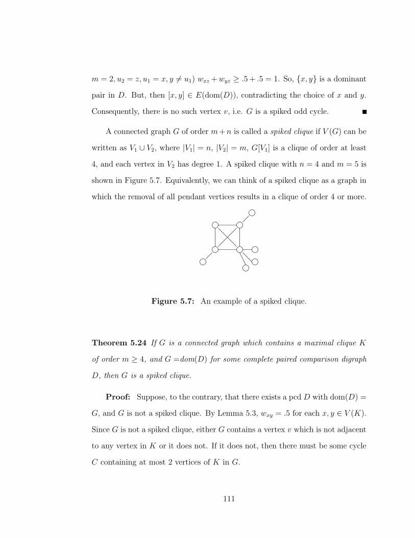
m = 2, u2 = z, u1 = x, y 6= u1) wxz + wyz ≥ .5 + .5 = 1. So, {x, y} is a dominant

pair in D. But, then [x, y] ∈ E(dom(D)), contradicting the choice of x and y.

Consequently, there is no such vertex v, i.e. G is a spiked odd cycle.

A connected graph G of order m+n is called a spiked clique if V (G) can be

written as V1 ∪ V2, where |V1| = n, |V2| = m, G[V1] is a clique of order at least

4, and each vertex in V2 has degree 1. A spiked clique with n = 4 and m = 5 is

shown in Figure 5.7. Equivalently, we can think of a spiked clique as a graph in

which the removal of all pendant vertices results in a clique of order 4 or more.

Figure 5.7: An example of a spiked clique.

Theorem 5.24 If G is a connected graph which contains a maximal clique K

of order m ≥ 4, and G =dom(D) for some complete paired comparison digraph

D, then G is a spiked clique.

Proof: Suppose, to the contrary, that there exists a pcd D with dom(D) =

G, and G is not a spiked clique. By Lemma 5.3, wxy = .5 for each x, y ∈ V (K).

Since G is not a spiked clique, either G contains a vertex v which is not adjacent

to any vertex in K or it does not. If it does not, then there must be some cycle

C containing at most 2 vertices of K in G.

111

First, suppose this cycle has order 3. If C and K share exactly 1 vertex

then C together with any pair of vertices of K form a bowtie. If C and K

share exactly 2 vertices, then C together with any vertex of K forms a chorded

4-cycle. From the proof of Theorem 5.22 we see that any bowtie or chorded

4-cycle must be contained in a clique. However, since the pair or single vertex

which forms the bowtie or chorded 4-cycle were chosen arbitrarily, each vertex

of C is adjacent to every vertex in K, a contradiction to K being maximal.

Now, the cycle cannot be of even length since this contradicts Theorem 5.20.

If the cycle is odd of order at least 5, then Theorem 5.23 assures us that G is

a spiked odd cycle, contradicting the existence of K in G. So, assume that

there exists v ∈ V (G) with v not adjacent to any vertex of K. Then, since G is

connected, there exists a shortest path P from K to v given by u1, u2, . . . , um = v

where m ≥ 3 and u1 ∈ V (K). We now show that {u2, x} is a dominant pair for

every x ∈ K to draw a contradiction.

Pick x ∈ V (K). First note, by Lemma 5.19, that wxy +wu2y = .5+ .5 = 1 for

all y ∈ V (K)−{x}. Now select z ∈ V (G)−V (K). By Lemma 5.19, wxz ≥ .5. We

show wu2z ≥ .5. If [z, u2] ∈ E(G), then since wu1z = .5, Lemma 5.19 and the fact

that {u1, u2} is a dominant pair implies that wu2z ≥ .5. If [u1, z] ∈ E(G), then

apply Lemma 5.1 to [z, u1] and [u2, u3] to see that wu2z = wu1u2 . Lemma 5.19

yields wu1u2 = .5, so wu2z = .5 as desired. Now, if z is not adjacent to u1

or u2 in G, then since G is connected, there exists a ∈ V (G) such that [z, a]

is in G. By applying Lemma 5.1 to the edges [u1, u2] and [z, a] we see that

wu2z = wzu1. By Lemma 5.19, wzu1 = .5 and so wu2z = .5 as desired. Thus, for

each z ∈ V (G) − V (K) wxz + wu2z ≥ .5 + .5 = 1. Thus, {x, u2} is a dominant

112

pair, a contradiction.

The previous two theorems show us that if D is a pcd such that dom(D)

is connected and contains an induced cycle or clique, then dom(D) is a spiked

odd cycle or a spiked clique. This together with the following lemma and some

results from the Section 5.3 will yield a classification of connected domination

graphs of pcds in Theorem 5.26.

Lemma 5.25 If G is a spiked clique, then there exists a complete paired com-

parison digraph D for which dom(D) = G.

Proof: Take the vertex set of D to be V (G). Let S denote the set of

vertices in V (G) that induces the clique in G. If [x, y] ∈ E(G) with x ∈ S and

y ∈ V (G) − S, define wxy = b, where .5 < b ≤ 1 (so, wyx = 1 − b). For all

other pairs of distinct vertices u and v in V (G) define wuv = .5. Pick distinct

x, y in V (G). We check that wxz + wyz ≥ 1 for all z ∈ V (G) − {x, y} if and

only if [x, y] ∈ E(G). Suppose that [x, y] ∈ E(G). If x, y ∈ S, then for all

z ∈ V (G) − {x, y},

wxz + wyz =

{

b + .5 , if z ∈ S and z is adjacent to x or y,.5 + .5 , otherwise.

If exactly one of x, y is in S, say x ∈ S and y 6∈ S, then for all z ∈ V (G)−{x, y},

wxz + wyz =

{

b + .5 , if [z, x] ∈ E(G), z 6∈ S,.5 + .5 , otherwise.

Since b > .5, wxz + wyz ≥ 1 for all z ∈ V (G) − {x, y}, as desired.

On the other hand, suppose that [x, y] 6∈ E(G). Since G is a spiked clique,

at least one of x, y is not in S, say y 6∈ S. Now, choose z ∈ S such that

113

[y, z] ∈ E(G). Then wyz = 1 − b, and since z ∈ S, wxz ≤ .5. So, wxz + wyz ≤

.5 + (1 − b) < .5 + .5 = 1. Thus, {x, y} is not a dominant pair, as desired.

Together, Lemma 5.25, and Theorems 5.13, 5.17, 5.20, 5.22, 5.23 and 5.24,

give us the following theorem classifying which connected graphs are the dom-

ination graphs of complete paired comparison digraphs. In comparison to the

analogous result for tournaments, Theorem 5.12, we see that there are several

new connected graphs which are the domination graphs of complete paired com-

parison digraphs, namely caterpillars without triple ends and spiked cliques.

Theorem 5.26 Let G be a connected graph. Then there exists a complete paired

comparison digraph D such that dom(D) = G if and only if G is a spiked odd

cycle, a caterpillar, or a spiked clique.

5.5 Domination graphs with no isolated vertices

Proposition 5.7 tells us that any graph can be an induced subgraph of the

domination graph of a pcd. However, in the proof, we essentially are carving

the desired graph from a clique, and leaving an isolated vertex in the graph for

each edge we delete. In this section we determine the graphs which comprise

the connected components of the domination graphs which contain no isolated

vertices, adding to the classes of the previous section the class of spiked bicliques.

We also show exactly which combinations of these classes are possible.

In light of Proposition 5.7, the results of this section essentially characterize

the basic graphs which can be the domination graphs of pcds. In the following

section we expand slightly on these results with some counting arguments for

114

obtaining graphs outside of this classification. We now open the section with

two results which limit the number of spiked cliques our graphs can contain.

Lemma 5.27 Let D be a complete paired comparison digraph. If K is a clique

of order 3 or more in dom(D) and [u, v] ∈ E(dom(D)) which is vertex disjoint

from K, then wzu = wzv = .5 for all z ∈ V (K).

Proof: Let K be a clique of order 3 or more in dom(D), and [u, v] ∈

E(dom(D)) which is vertex disjoint from K. Choose distinct vertices x, y, z ∈

V (K). Since K is a clique, [x, y], [y, z], [x, z] ∈ E(dom(D)). So, by Lemma 5.1,

wxu = wuy = wyv = wvx,

wxu = wuz = wzv = wvx, and

wuy = wyv = wvz = wzu.

So, wzv = wxu = wyv = wvz = 1−wzv, and so wuz = wzv = .5. Since x, y, z were

chosen arbitrarily from V (K), the result holds.

Theorem 5.28 Let D be a complete paired comparison digraph such that

dom(D) has no isolated vertices. Then, dom(D) does not contain more than

one maximal clique of size at least four.

Proof: Suppose to the contrary that there exist two maximal cliques of

size 4 or more. Let K1 and K2 denote the sets of vertices which induce these

cliques. Let D1 and D2 be the pcds induced on K1 and K2 respectively. Since

K1 and K2 induce cliques in dom(D), by Theorem 5.4, dom(D1) and dom(D2)

must also be cliques. So, by Lemma 5.3, wxy = .5 for all x, y ∈ K1 and x, y ∈ K2.

We show wxy = .5 for all x, y ∈ K1 ∪ K2.

115

If K1 ∩K2 = ∅, then by Lemma 5.27, wxy = .5 for each x ∈ K1 and y ∈ K2,

and so wxy = .5 for each x, y ∈ K1∪K2. So, assume K1∩K2 6= ∅. First consider

when |K1 ∩ K2| = 1. Let a be the unique vertex in K1 ∩ K2. Then K1 − {a}

and K2 − {a} induce disjoint cliques of order 3 or more. So, by Lemma 5.27,

wxy = .5 for all x ∈ K1 − {a} and y ∈ K2 − {a}. So, since wxa = wya = .5,

for all x ∈ K1 and y ∈ K2, wxy = .5 for all x ∈ K1, and y ∈ K2. Now,

assume |K1 ∩ K2| ≥ 2. Choose distinct vertices b, c ∈ K1 ∩ K2, x ∈ K1 − K2

and y ∈ K2 − K1. Then [x, b] and [y, c] are disjoint edges in dom(D), and

so by Lemma 5.1 wxy = wyb = wbc = wcx. Since b ∈ K2, wyb = .5, and so

wxy = .5. Since x and y were chosen arbitrarily, wxy = .5 for all x ∈ K1 − K2

and y ∈ K2 − K1. Thus, wxy = .5 for all x, y ∈ K1 ∪ K2.

If V (D) = K1 ∪ K2 then wxz + wyz = 1 for all x, y, z ∈ V (D), so {x, y} is

a dominant pair for all x, y ∈ V (D), and dom(D) is a complete graph, contra-

dicting dom(D) having two maximal cliques. So, assume V (D) 6= K1 ∪K2, and

let v ∈ V (D) − (K1 ∪ K2). Since dom(D) has no isolated vertices, there exists

u ∈ V (D) such that [u, v] ∈ E(dom(D)). If u ∈ K1 ∪ K2, then by Lemma 5.19

(with m = 2), wva = .5 for all a ∈ K1∪K2−{u} and wuv ≥ .5. If [u, v] is disjoint

from K1 ∪ K2, then by Lemma 5.27, wxv = .5 for all x ∈ K1 and wyv = .5 for

all y ∈ K2. Thus, wxv + wyv ≥ .5 + .5 = 1 for all x, y ∈ K1 ∪ K2. Since v was

chosen arbitrarily, this is true for all v ∈ K1∪K2. Further, since wxy = .5 for all

x, y ∈ K1 ∪ K2, wxz + wyz = 1 for all x, y, z ∈ K1 ∪ K2. Thus, K1 ∪ K2 induces

a clique in dom(D), a contradiction to K1 and K2 inducing maximal cliques in

dom(D).

116

Theorem 5.29 Let D be a complete paired comparison digraph, and let G be

a component of dom(D). Let D′ be the complete paired comparison digraph

induced on the vertices of G. If G is not a spiked odd cycle or a caterpillar, then

dom(D′) is a spiked clique.

Proof: From Theorem 5.4, Theorem 5.26 and the fact that G is connected,

we know that dom(D) must be a subgraph of a spiked odd cycle, a caterpillar,

or a spiked clique. Subgraphs of spiked odd cycles and caterpillars are spiked

odd cycles and caterpillars. So, if G is neither of these, we must have dom(D′)

is a spiked clique.

Lemma 5.30 Let D be a complete paired comparison digraph such that some

component S of dom(D) contains an odd cycle C, and let [x, y] be an edge of

dom(D) which is vertex disjoint from C. Then in D, wvx = wvy = .5 for each

v ∈ V (S).

Proof: Pick a vertex in C and call it c1, then trace all other vertices in C

in a clockwise order, labeling them c2, c3, . . . , c2k+1. From Lemma 5.1 applied to

the edges [x, y] and [c1, c2], wxc1 = wc1y = wyc2 = wc2x. Also, Lemma 5.1 applied

to [c2, c3] and [x, y] gives wc2x = wxc3 = wc3y = wyc2. Now choose i and assume

that for each odd j < i,

wxc1 = wxcj= wcjy = wycj+1

= wcj+1x.

Then, by Lemma 5.1 applied to [x, y] and [ci−1, ci],

wxc1 = wci−1x = wxci= wciy = wyci−1

.

117

So, by induction,

wxc1 = wxci= wciy = wyci+1

= wci+1x

for all odd i. In particular, wxc2k+1= wxc1, and from Lemma 5.1 applied to [x, y]

and [c2k+1, c1] we have that

wxc2k+1= wxc1 = wc1y = wyc2k+1

= wc2k+1x = 1 − wxc2k+1.

Thus, wxc1 = wc1x = .5, and so wxv = wyv = .5 for all v ∈ C.

If V (C) = V (S) we are done, so assume that there exists a vertex v ∈

V (S) − V (C). Then, since S is a connected component of dom(D), there is

a shortest path P from C to v given by u1, u2, . . . , um where um = v. From

Lemma 5.1 applied to the pairs [x, y] and [u1, u2],

.5 = wxc1 = wxu1 = wu1y = wyu2 = wu2x.

Now, assume that wxuj= wyuj

= .5 for all j ≤ i. Then Lemma 5.1 applied to

the pairs [ui, ui+1] and [x, y] yields

wxui+1= wui+1y = wyui

= .5

and so wyui+1= 1 − wui+1y = 1 − .5 = .5. Thus, for all ui, wxui

= wyui= .5.

In particular, wxv = wyv = .5. Since v was arbitrary, this holds for all v ∈

V (S) − V (C). Thus, wvx = wvy = .5 for all v ∈ V (S).

Theorem 5.31 Let G be a graph with no isolated vertices, which contains a

component S which contains an odd cycle, and S is not a spiked odd cycle or

spiked clique. There does not exist a complete paired comparison digraph D such

that dom(D) = G.

118

Proof: Suppose to the contrary, that there exists a pcd D such that

dom(D) = G. If G = S, then from Theorem 5.26 the result follows, so suppose

G has more than one component. Let D′ be the pcd induced on V (S). Then,

from Theorem 5.29, dom(D′) is a spiked clique. Let H be the subset of vertices

of S which are not pendant in dom(D′). Then, for all x, y ∈ H, wxy = .5, by

Lemma 5.3, and since [x, y] ∈ E(dom(D′)), wxz + wyz ≥ 1 for all x, y ∈ H, and

z ∈ V (S).

Now, choose v ∈ V (G) − V (S). Since G has no isolated vertices there

exists u ∈ V (G) − V (S) such that [u, v] ∈ E(G). From Lemma 5.30 we know

that wus = wvs = .5 for all s ∈ V (S). So, for each x, y ∈ H, we have that

wxv + wyv ≥ 1 for all v ∈ V (G) − {x, y}. Thus, H induces a clique in dom(D).

By Theorem 5.4, S is a subgraph of dom(D′). So, since dom(D′) is a spiked

clique, with its clique induced on H, and H induces a clique in dom(D), S must

be a spiked clique when |H| ≥ 4, and a spiked 3-cycle when |H| = 3. This

contradicts the choice of S, so no such pcd exists.

Recall a graph is bipartite if and only if it contains no odd cycles. This gives

the following corollary.

Corollary 5.32 Let D be a complete paired comparison digraph. If dom(D)

has no isolated vertices, then any component which is not a spiked odd cycle or

spiked clique is bipartite.


dom(D) has no isolated vertices and dom(D) contains a component which is

not a caterpillar, spiked odd cycle, or spiked clique. Then dom(D) has at least

119

two bipartite components.

Proof: Let S be the component which is neither a caterpillar, spiked odd

cycle, or spiked clique. From Theorem 5.26 we know that dom(D) must have

another component, and from Corollary 5.32 we know that S is bipartite. So,

suppose to the contrary, that no other component is bipartite. Then every other

component of dom(D) contains an odd cycle. Since S is connected, for each

x ∈ V (S) there exists a y in S such that [x, y] ∈ E(S). So, since all components

of dom(D) other than S contain an odd cycle, wxv = .5 for all x ∈ V (S) and

v 6∈ V (S) by Lemma 5.30. Now, from Theorem 5.29 we know that the pcd D′

induced on S has a spiked clique as its domination graph. Let H denote the

vertices which form the clique in dom(D′). Note |H| ≥ 4 by definition of spiked

clique. Then wxv +wyv ≥ 1 for all x, y ∈ H and v ∈ V (S). Thus, for all x, y ∈ H

and v ∈ V (D), wxv + wyv ≥ 1, and so H is a clique in dom(D). A contradiction

to S being bipartite. Thus, there must exist some other component of dom(D)

which does not contain an odd cycle, and so dom(D) contains at least 2 bipartite

components.

Lemma 5.34 Let D be a complete paired comparison digraph. Suppose that

dom(D) contains a bipartite component B. Let X ∪ Y be the bipartition of B,

and u, v ∈ X. Then, wuz = wvz for each vertex z ∈ V (D)− V (B) such that z is

not isolated in dom(D). Also, wac = wbc for each a, b ∈ Y , and c ∈ V (D)−V (B)

such that c is not isolated in dom(D).

Proof: Choose u, v ∈ X and z ∈ V (D)−V (B) such that z is not isolated.

Since z is not an isolated vertex in dom(D), B is a component and z 6∈ V (B),

120

there must exist a y ∈ V (D) − V (B) such that [y, z] is an edge of dom(D).

Since B is connected, there exists a path P from u to v in dom(D) given by

u1, u2, . . . , um where u = u1 and um = v. Since B is bipartite, for all odd i,

ui ∈ X and ui+1 ∈ Y . Note, since v ∈ X, m is odd. Now, from Lemma 5.1,

wuz = wzu2 = wu2y = wyu1. So, assume that for each odd i, wuz = wuiz =

wzui+1= wui+1y = wyui

. Lemma 5.1 applied to [z, y] and [ui+1, ui+2] gives wuz =

wui+1y = wyui+2= wui+2z. Thus, for all odd i, wuiz = wuz. So, wvz = wuz. Since

z was chosen arbitrarily wuz = wvz for all u, v ∈ X, and v 6∈ V (B) with v not

isolated. By symmetry, wac = wbc for each a, b ∈ Y , and c ∈ V (D)− V (B) such

that c is not isolated in dom(D). This completes the proof.

Theorem 5.35 Let D be a complete paired comparison digraph, and let G and

H be non-trivial bipartite components of dom(D) with bipartitions V (G) = G1 ∪

G2 and V (H) = H1 ∪ H2. Then for i, j ∈ {1, 2}, for all distinct u, u′ ∈ Gi, and

for all distinct v, v′ ∈ Hj, wuv = wu′v′ .

Proof: Pick i, j ∈ {1, 2}. From Lemma 5.34 we know that wuz = wu′z for

all u, u′ ∈ Gi and z ∈ V (H). Furthermore, wvz = wv′z for each v, v′ ∈ Hj and

z ∈ V (G). Thus,

wuv = 1 − wvu = 1 − wv′u = wuv′ = wu′v′

for all u, u′ ∈ Gi and v, v′ ∈ Hj.

We define a spiked biclique as a graph G such that the graph obtained

by removing all pendant vertices of G is a biclique. Some examples of spiked

bicliques are shown in Figure 5.8. Note bicliques themselves are spiked bicliques.

So, the smallest spiked biclique is the single edge.

121

Figure 5.8: Some spiked bicliques


dom(D) contains no isolated vertices. Any component of dom(D) which is not

a spiked odd cycle, spiked clique or caterpillar, is a spiked biclique.

Proof: Let G be a component of dom(D) which is not a spiked odd cycle,

spiked clique or caterpillar. From Corollary 5.32 we know that G is bipartite with

bipartition X∪Y . Now, dom(D) must contain another component for otherwise

dom(D) = G, a contradiction to Theorem 5.26. Let H be the subgraph of G

formed by removing the pendant vertices of G. Note H is connected, and if

|V (H)| > 1, H is a bipartite graph, with bipartition (X ∩ V (H))∪ (Y ∩ V (H)).

Suppose, to the contrary, [x, y] 6∈ E(H) for some x ∈ X ∩ V (H) and y ∈

Y ∩ V (H). So there must be some vertex of D, call it v, so that wxv + wyv < 1.

Let D′ be the pcd induced on V (G). Since G is not a spiked odd cycle or

caterpillar, dom(D′) is a spiked clique by Theorem 5.29. Since H is obtained

by removing the pendant vertices of G, V (H) is contained within the vertices

of dom(D′) which induce the clique. Hence, wxu + wyu ≥ 1 for all x, y ∈ V (H)

and v ∈ V (G). So, v ∈ V (D) − V (G). By Lemma 5.30, if u is in a component

of dom(D) containing an odd cycle wxu + wyu = .5 + .5 = 1. So, v must be in

122

some bipartite component, K, of dom(D).

By Lemma 5.34, wxv = wx′v′ for all x′ ∈ X∩V (H) and v′ ∈ V (K). Similarly,

wyv = wy′v′ for all y′ ∈ Y ∩ V (H) and v′ ∈ V (K). Thus, since wxv + wyv < 1,

wx′v′ + wy′v′ < 1 for all x′ ∈ X ∩ V (H), y′ ∈ Y ∩ V (H), and v′ ∈ X0. So,

E(H) = ∅. Since H is a connected graph, H must be a single vertex. Since H

is the graph obtained from G by removing the pendant vertices of G, G must

be a star. However, this implies that G is a caterpillar, a contradiction to our

choice of G. Thus, [x, y] ∈ E(H) for all x ∈ X ∩ V (H) and y ∈ Y ∩ V (H), and

so G is a spiked biclique.

The spiked biclique is an interesting new class which not only increases

the kinds of graphs which can can be domination graphs of pcds from the last

section, but puts quite a bit of distance between the domination graphs of pcds

and the domination graphs of tournaments. Recall that a tournament cannot

have an even cycle or NC7 in its domination graph. However, since the 4-cycle

is a biclique, it can be the domination graph of a pcd. Also, NC7 is a spiked

biclique (in fact, it is the graph on the right in Figure 5.8), so NC7 can be the

domination graph of a pcd. So, the trees which are the domination graphs of

pcds do not necessarily need to be caterpillars. However, trees which are not

caterpillars must be spiked bicliques, and hence are fairly restricted.

Lemma 5.37 Let G be a star on n ≥ 3 vertices with center u. Then there exists

a complete paired comparison digraph, D, such that O+(u) 6= V (D) − {u} and

dom(D) = G.

Proof: We construct D as follows. Let V (D) = V (G). Let p and p′ be

123

real numbers so that .5 < p′ < p < 1. Choose v ∈ V (D)−{u}, and set wvu = p′,

and wuv = 1 − p′. For x ∈ V (D) − {u, v} set wux = p and wxu = 1 − p, and set

wxv = p′ and wvx = 1 − p′. For each x, y ∈ V (D) − {u, v} set wxy = p or 1 − p

arbitrarily, to create a pcd. We claim dom(D) = G.

Let x, y ∈ V (D)−{u, v}. If x 6= y then wuy + wxy is p + (1− p) or p + p. In

either case wuy + wxy ≥ 1, since p > .5. Also, wuv + wxv = 1 − p′ + p′ = 1. So,

[u, x] ∈ E(dom(D)) for each x ∈ V (D) − {u, v}. Now, wux + wvx = p + p′ > 1

for each x ∈ V (D) − {u, v}, so [u, v] ∈ E(dom(D)). So, E(G) ⊆ E(dom(D)).

By Lemma 5.5, O+(u) = V (D) − {u, v} is an independent set in dom(D). So,

we need only show that [v, x] is not an edge for x ∈ V (D)−{u, v}. This follows

since wvu + wxu = p′ + 1 − p = 1 − (p − p′) < 1. So, dom(D) = G.

Lemma 5.38 Let G be a spiked odd cycle or caterpillar on 3 or more vertices.

There exists a complete paired comparison digraph D so that dom(D) = G, and

if u ∈ V (D) there is some v ∈ V (D) so that wuv < .5.

Proof: Suppose that no such pcd exists. By Theorem 5.26, there exists

a pcd D so that dom(D) = G. So for every such D there must be some vertex

u ∈ V (D) so that O+(u) = V (D) − {u}. By Lemma 5.5, V (D) − {u} forms an

independent set in dom(D). So, since G is a caterpillar or spiked odd cycle, G

must be a star centered at u. So, for every pcd such that dom(D) is a star on

n ≥ 3 vertices, O+(u) = V (D) − {u}, where u is the center of the star. This is

a contradiction to Lemma 5.37. So such a pcd must exist.

Lemma 5.39 Let G be a graph with no isolated vertices whose connected com-

ponents form some collection of the following:

124

1. At most one spiked clique.

2. Spiked odd cycles.

3. Caterpillars on 3 or more vertices.

Then, there exists a complete paired comparison digraph D such that dom(D) =

G. Further, for each vertex u of D not contained in the spiked clique, there

exists a vertex v so that wuv < .5.

Proof: We construct D as follows. Let V (D) = V (G). Let C1, . . . , Ck

denote the caterpillars of G. Let K denote the spiked clique in G. Let

S1, . . . , Sm denote the spiked odd cycles of G. Note we only require at

least one of C1, . . . , Ck, K, S1, . . . , Sm exist. By Theorem 5.26, there exists

a pcd DK such that dom(DK) = K. Also, by Lemma 5.38 there exist

pcds DC1 , . . . , DCk, DS1, . . . , DSm

so that for i = 1, . . . , k and j = 1, . . . , m

dom(DCi) = Ci and for every vertex u of DCi

there exists a vertex v of DCi

so that wuv < .5, and dom(DSj) = Sj and for each x ∈ V (DSj

) there exists a

y ∈ V (DSj) so that wxy < .5. Weight the arcs in D so that V (K) induces DK,

V (Ci) induces DCifor i = 1, . . . , k and V (Sj) induces DSj

for j = 1, . . . , m.

Give the remaining arcs of D weight .5. We claim dom(D) = G.

Let D′ ∈ {DC1 , . . . , DCk, DK, DS1 , . . . , DSm

}. If [x, y] ∈ E(dom(D′)), then

wxv+wyv ≥ 1 for all v ∈ V (D′). Also, wxz+wyz = .5+.5 = 1 for each z 6∈ V (D′).

If [x, y] 6∈ E(dom(D′)), then by Theorem 5.4, [x, y] 6∈ E(dom(D)). So each of

C1, . . . , Ck, K, S1, . . . , Sm are induced subgraphs of dom(D). Note, if G has only

one component we are done. So, assume G has 2 or more components, and pick

u, v ∈ V (D) so that u and v are in separate components of G. So, at most one

125

of u, v can be in K, and without loss of generality, say u is not in K. So u is in

one of C1, . . . , Ck, S1, . . . , Sm. Let D′′ ∈ {DC1 , . . . , DCk, DK, DS1 , . . . , DSm

} so

that u ∈ V (D′′). By Lemma 5.38, there is some t ∈ V (D′′) so that wut < .5.

Thus, wvt + wut < .5 + .5 = 1, and [u, v] 6∈ E(dom(D)). Thus, dom(D) = G.

Note that in proving the construction above we did not require the existence

of any particular component.

Lemma 5.40 Let G be a graph with exactly two components, one of which is

a spiked clique and the other is a single edge. There does not exist a complete

paired comparison digraph whose domination graph is G.

Proof: Suppose there exists a pcd, D, with dom(D) = G. Let K be

the set of vertices which induce the spiked clique in dom(D), and {u, v} the

set of vertices which induce the single edge. Without loss of generality, assume

wuv ≥ wvu. Let K ′ be the set of vertices in K which induce the clique. By

Lemma 5.27, wxu = wxv = .5 for all x ∈ K ′. If y ∈ K − K ′, and z is the vertex

adjacent to y in dom(D), then z ∈ K and by Lemma 5.1, wuy = wyv = wvz = .5.

So, wut = wvt = .5 for all t ∈ K. So, wus + wts ≥ 1 for all t ∈ K and

s ∈ V (D) − {u, t}. Thus, [u, t] ∈ E(dom(D)) for each t ∈ K, and dom(D) is

connected, a contradiction. Thus no such pcd exists.

Lemma 5.41 Let G be a graph with exactly two components, one of which is

a spiked odd cycle, and the other is a single edge. Then there exists a complete

paired comparison digraph D so that dom(D) = G.

Proof: Construct D as follows. Let V (D) = V (G). Let S denote the

spiked odd cycle of G, and let [u, v] be the single edge component of G. By

126

Lemma 5.38, there exists a pcd D1 so that dom(D1) = S, and for all u ∈ V (D1)

there exists a v ∈ V (D1) so that wuv < .5. Let V (S) induce D1 and set all other

arc weights to .5. We claim dom(D) = G.

Pick [x, y] ∈ E(S). Then wxz + wyz ≥ 1 for all z ∈ V (D1), and wxa + wya =

.5 + .5 = 1 for each a 6∈ V (D1). Thus [x, y] ∈ E(dom(D)). If [s, t] 6∈ E(S),

then [s, t] 6∈ E(dom(D1)), and so [s, t] 6∈ E(dom(D)) by Theorem 5.4. Now, for

each z ∈ V (D1), wuz + wvz = .5 + .5 = 1, and since V (D1) = V (D) − {u, v},

[u, v] ∈ E(dom(D)). Also, if b ∈ V (D1), there exists c ∈ V (D1) so that wbc < .5.

So, wuc+wbc = wvc+wbc < 1, and [u, b], [v, b] 6∈ E(dom(D)). Thus, dom(D) = G.

Lemma 5.42 Let G be a graph with at least two components each of which is

a spiked biclique. Then there exists a complete paired comparison digraph D so

that for all u ∈ V (D) there exists some v ∈ V (D) such that wuv < .5, and

dom(D) = G.

Proof: Construct D as follows. Let V (D) = V (G). Let S1, . . . , Sk be the

components of G, and let Xi∪Yi be the bipartition of Si for i = 1, . . . , k. Choose

.5 < p < 1. For i < j weight the arcs of D as follows. For x ∈ Xi, x′ ∈ Xj,

y ∈ Yi and y′ ∈ Yj set

wxx′ = p, wx′x = 1 − p,

wyy′ = p, wy′y = 1 − p,

wy′x = p, wxy′ = 1 − p,

wx′y = p, and wyx′ = 1 − p.

127

For each i = 1, . . . , k let S ′i denote the biclique of Si. For each i = 1, . . . , k,

and each distinct u, v ∈ V (S ′i), set wuv = .5. For each a ∈ V (Si) − V (S ′

i) let

b be its unique neighbor in Si, and set wba = p, wab = 1 − p, and wau = .5 for

each u 6= b in Si. Note from our construction, for each u ∈ V (Si), there is some

vertex v ∈ V (Sj) with i 6= j so that wuv = 1 − p < .5. So, for each u ∈ V (D)

there is some v ∈ V (D) such that wuv < .5. We finish by showing dom(D) = G.

Let [u, v] ∈ E(G), and say [u, v] ∈ E(Sj). Pick z ∈ V (D)− {u, v}. Suppose

z ∈ V (Sj). If z is not a pendant vertex adjacent to either of u or v in Sj, then

wuz + wvz = .5 + .5 = 1. If z is a pendant vertex adjacent to one of u or v in Sj,

then wuz + wvz = .5 + p > 1. Now suppose z 6∈ V (Sj). Since Sj is bipartite, one

of u, v is in Xj and the other is in Yj. Without loss of generality, assume u ∈ Xj

and v ∈ Yj. Since z 6∈ V (Sj), z ∈ V (Si) for some i 6= j. Since Si is bipartite,

z ∈ Xi or z ∈ Yi. If z ∈ Xi, then wuz + wvz = (1 − p) + p = 1 for i < j and

wuz +wvz = p+(1− p) = 1 for i > j. If z ∈ Yi, then wuz +wvz = p+(1− p) = 1

for i < j and wuz + wvz = (1 − p) + p = 1 for i > j. Thus, [u, v] ∈ E(dom(D)),

and E(G) ⊆ E(dom(D)).

Now pick [u′, v′] 6∈ E(G). First suppose u′, v′ ∈ V (Si) for some i. Suppose

u′ and v′ are in the same bipartition of Si. If u′, v′ ∈ Xi, then for every a ∈ Xq

and b ∈ Yr, with q < i < r, u′, v′ ∈ O+(a) and u′, v′ ∈ O+(b). Note, since

G has at least two components, at least one of Xq and Yr must exist. So,

[u′, v′] 6∈ E(dom(D)) by Lemma 5.5. So, assume u′ and v′ are in different

bipartitions of Si. Then either u′ or v′ is a pendant vertex of Si. Without loss

of generality, assume v′ is the pendant, and c is its unique neighbor in Si. Since

[u, v] 6∈ E(Si), c 6= u, so wuc + wvc = .5 + (1 − p) < 1. So, [u′, v′] 6∈ E(dom(D)).

128

Now suppose u′ ∈ V (Si) and v′ ∈ V (Sj) for some i < j. If u′ ∈ Xi and v′ ∈ Xj,

then since Yj must be non-empty there is some y ∈ Yj so that wu′y + wv′y =

(1 − p) + .5 < 1. If u′ ∈ Yi and v′ ∈ Yj, then there is some x ∈ Xj, so that

wu′x+wv′x = (1−p)+ .5 < 1. If u′ ∈ Xi and v′ ∈ Yj, then there is some y ∈ Yi so

that wu′y +wv′y = .5+ (1− p) < 1. Finally, if u′ ∈ Yi, and v′ ∈ Xj, then there is

some x ∈ Xi so that wu′x + wv′x = .5 + (1− p) < 1. Thus, [u′, v′] 6∈ E(dom(D)),

and dom(D) = G.

Lemma 5.43 Let G be a graph with at least two components, each of which is a

caterpillar or a spiked biclique. Then there exists a complete paired comparison

digraph D so that dom(D) = G, and for each u ∈ V (D), there exists v ∈ V (D)

so that wuv < .5.

Proof: Note, if every component of G is a caterpillar, then the result

follows from Lemma 5.15, so assume G has at least one component which is a

spiked biclique. Construct D as follows. Let V (D) = V (G). Let S1, . . . , Sm be

the spiked bicliques of G including single edges, but not stars. Let C1, . . . , Ck be

the caterpillars of G including stars, but not including single edges. We consider

two cases. By Lemma 5.39, there exists a pcd, DC , so that for each u ∈ V (DC)

there exists a v ∈ V (DC) so that wuv < .5 and dom(DC) = C1 ∪ C2 ∪ · · · ∪ Ck.

Let q = max{wab : a, b ∈ V (DC)}. Note, by Lemma 5.6 we may assume q < 1.

Weight the arcs of D so that V (C1), . . . , V (Ck) induce DC . We consider two

cases. In the first m ≥ 2, and in the second m = 1 and k ≥ 1. If m ≥ 2, then

by Lemma 5.42, there exists a pcd DS so that dom(DS) = S1 ∪ S2 ∪ · · · ∪ Sm.

Weight the arcs of D so that V (S1) ∪ V (S2) ∪ · · · ∪ V (Sm) induce DS. In the

129

case where m = 1, let S ′1 denote the biclique of S1. For each x, y ∈ V (S ′

1) set

wxy = .5. Let l be a real number such that .5 < l < 1. If a ∈ V (S1)−V (S ′1), let

b be its unique neighbor in S1 and set wba = l, wab = 1 − l and set wac = .5 for

each c ∈ V (S1) − {a, b}.

For both the case m = 1 and m ≥ 2, let Xi ∪ Yi denote the bipartition of Si

for i = 1, . . . , m, and let X ′j ∪ Y ′

j denote the bipartition of Cj for j = 1, . . . , k.

Choose a real number p with q < p < 1. For i = 1, . . . , m, j = 1, . . . , k, x ∈ Xi,

x′ ∈ X ′j, y ∈ Yi and y′ ∈ Y ′

j , set

wx′x = p, wxx′ = 1 − p,

wy′y = p, wyy′ = 1 − p

wxy′ = p, wy′x = 1 − p

wyx′ = p, and wx′y = 1 − p

So, if u ∈ V (Si) for some i, then there is some v ∈ V (DC) so that wuv < .5. So,

for all u ∈ V (D) there exists some v ∈ V (D) so that wuv < .5, and if u ∈ V (DC)

there exists v ∈ V (DC) so that wuv < .5 by Lemma 5.39. We finish the proof

by showing dom(D) = G.

Pick [u, v] ∈ E(G). First suppose [u, v] ∈ E(Cj) for some j. Then, since

dom(DC) = C1 ∪ C2 ∪ · · · ∪ Ck, wuz + wvz ≥ 1 for each z ∈ V (DC). Also, if

z 6∈ V (DC), then z ∈ V (Si) for some i, and so wuz + wvz = p + (1 − p) = 1,

and [u, v] ∈ E(dom(D)). Now suppose [u, v] ∈ E(Si) for some i. If m ≥ 2,

then since dom(DS) = S1 ∪ · · · ∪ Sm, wuz + wvz ≥ 1 for each z ∈ V (DS), and

wuz′ + wvz′ = p + (1 − p) for each z′ ∈ V (DC), so [u, v] ∈ E(dom(D)). Now,

consider when m = 1. Pick z ∈ V (S1). If z is not a pendant vertex adjacent to

130

either of u or v in S1, then wuz + wvz = .5 + .5 = 1. If z is a pendant vertex

adjacent to one of u or v in Sj, then wuz + wvz = .5 + l > 1. If z′ 6∈ V (S1), then

wuz′+wvz′ = p+(1−p) = 1. Thus, [u, v] ∈ E(dom(D)). So E(G) ⊆ E(dom(D)).

Now pick distinct u′, v′ ∈ V (D) so that [u′, v′] 6∈ E(G). If u′, v′ ∈ V (DC),

then [u′, v′] 6∈ E(dom(D)) by Theorem 5.4. Similarly, in the case where m ≥ 2,

if u′, v′ ∈ V (DS), then [u′, v′] 6∈ E(dom(D)) by Theorem 5.4. Consider the

case where m = 1. If u′, v′ ∈ V (S1), then since [u′, v′] 6∈ E(S1), either u′ and

v′ are in the same bipartition of S1 or one of u′ or v′ is pendant in S1. If u′

and v′ are in the same bipartition of S1 then there is some x ∈ V (DC) so that

wu′x + wv′x = 1 − p + 1 − p < 1. So, without loss of generality, assume v ′ is a

pendant in S1, and y is its unique neighbor in S1. Then since [u, v] 6∈ E(S1),

y 6= u and wu′y + wv′y = .5 + (1 − l) < 1. So, [u′, v′] 6∈ E(dom(D)). Now, for

both cases, assume u′ ∈ V (Si) for some i and v′ ∈ V (Cj) for some j. If u′ ∈ Xi

and v′ ∈ X ′j, then since Yj must be non-empty there is some y ∈ Yj so that

wu′y + wv′y = .5+ (1− p) < 1. If u′ ∈ Yi and v′ ∈ Y ′j , then there is some x ∈ Xi,

so that wu′x + wv′x = .5 + (1 − p) < 1. If u′ ∈ Xi and v′ ∈ Y ′j , then there is

some x ∈ X ′j so that wu′x + wv′x ≤ q + (1 − p) < 1. Finally, if u′ ∈ Yi, and

v′ ∈ X ′j, then there is some y ∈ Y ′

j so that wu′y + wv′y ≤ (1 − p) + q < 1. Thus,

[u′, v′] 6∈ E(dom(D)), and dom(D) = G.

Lemma 5.44 Let G be a graph with no isolated vertices and at least 3 compo-

nents which form some collection of the following.

1. At most one spiked clique.

2. Spiked odd cycles.

131

3. At least two bipartite graphs consisting of spiked bicliques and caterpil-

lars.

There exists a complete paired comparison digraph D so that dom(D) = G.

Proof: Construct D on the vertices of G by assigning weights in the

following ways. Let G1 be the induced subgraph of G which consists of the

spiked clique and spiked odd cycles of G. By Lemma 5.39, there exists a pcd

D1 so that dom(D1) = G1. Let G2 be the induced subgraph of G which consists

of spiked bicliques and caterpillars. If G2 = ∅, then the result follows from

Lemma 5.39. So, assume G2 6= ∅. By Lemmas 5.38, 5.42 and 5.43, (depending

on if G contains a just caterpillars, just spiked bicliques, or both) there exists

a pcd D2 so that for each u ∈ V (D2) there exists a vertex v ∈ V (D2) such

that wuv < .5, and dom(D2) = G2. Note, if G1 = ∅, the result follows from

Lemma 5.38, 5.42 or 5.43. So, assume G1 6= ∅. Weight the arcs of D so that

V (G1) induces D1, V (G2) induces D2 and wxy = .5 for all x ∈ V (G1) and

y ∈ V (G2). We claim dom(D) = G.

Pick [u, v] ∈ E(G). If u, v ∈ V (G1), then since dom(D1) = G1, wuz+wvz ≥ 1

for all z ∈ V (G1) − {u, v}. Also, if z 6∈ V (G1), wuz + wvz = .5 + .5 = 1.

So, [u, v] ∈ E(dom(D)). By a symmetric argument, if u, v ∈ V (G2), then

[u, v] ∈ E(dom(D)). So, E(G) ⊆ E(dom(D)). Now, pick u′, v′ ∈ V (D) so

that [u′, v′] 6∈ E(G). If u′, v′ ∈ V (G1), then [u′, v′] 6∈ E(dom(D1)), and so

[u′, v′] 6∈ E(dom(D)) by Theorem 5.4. If u′, v′ ∈ V (G2), then by a similar

argument, [u′, v′] 6∈ E(dom(D)). So, assume u′ ∈ V (G1) and v′ ∈ V (G2). By

our construction, there exists some z ∈ V (G2) so that wv′z < .5. So, wu′z+wv′z <

132

.5 + .5 = 1. So, [u′, v′] 6∈ E(dom(D)), and dom(D) = G.

We now state our main results.

Theorem 5.45 Let G be a graph with exactly two components and no isolated

vertices. Then there exists a complete paired comparison digraph D such that

dom(D) = G if and only if the components of G are one of the following.

1. two spiked odd cycles,

2. a spiked odd cycle and a caterpillar,

3. two caterpillars,

4. two spiked bicliques,

5. a spiked clique and a spiked odd cycle,

6. a spiked clique and a caterpillar other than a single edge,

7. a caterpillar and a spiked biclique.

Proof: The necessary conditions follow from Theorems 5.28, 5.33, and

5.36, and Lemma 5.40. Sufficiency follows from Lemmas 5.39, 5.41 5.42, and

5.43.

Theorem 5.46 Let G be a graph with n ≥ 3 non-trivial components and no

isolated vertices. There exists a complete paired comparison digraph D with

dom(D) = G if and only if G is one of the following:

1. A spiked clique together with any collection of n − 1 spiked odd cycles

and caterpillars.

133

2. Any collection of n spiked odd cycles and caterpillars.

3. A spiked clique, any collection of spiked odd cycles, and a set of two or

more bipartite graphs containing only spiked bicliques and caterpillars.

4. Any collection of spiked odd cycles, and a set of two or more bipartite

graphs containing only spiked bicliques and caterpillars.

Proof: The necessary conditions come from Theorems 5.28, 5.33, and 5.36.

The sufficient conditions come from Lemmas 5.39 and 5.44.

5.6 Isolated vertices in domination graphs

We have a characterization of the graphs which can be the domination

graphs of complete paired comparison digraphs when we do not allow isolated

vertices in the domination graph. We have also seen that any graph can be

an induced subgraph of the domination graph of a complete paired compari-

son digraph. We conclude this chapter with a lower bound on the number of

isolated vertices necessary in the domination graph of a pcd in order to have

a graph which did not appear in the previous section’s characterization in the

domination graph.

Recall from Lemma 5.5, that for a vertex v in a pcd, O+(v) forms an indepen-

dent set in the domination graph. An independent set in a graph G corresponds

to a clique in the complement of G. So if we want to carve G out of a spiked

clique, we are essentially looking to remove cliques from G using O+(v) for var-

ious vertices v. With this strategy we obtain our lower bound using the edge

clique cover number of the complement of G. A clique covering of a graph H is

134

a collection of cliques Q1, Q2, . . . , Qm contained in H such that each edge of H

is in some Qi. The edge clique cover number of a graph H, denoted θ(H), is the

size of a minimum clique covering of H.

Theorem 5.47 Let G be a connected graph which is not a spiked clique, spiked

odd cycle, caterpillar or spiked biclique. Let H be the graph obtained from G

by removing the pendant vertices from G. If G is a component of dom(D) for

some complete paired comparison digraph D, then dom(D) contains at least θ(H)

isolated vertices.

Proof: Let D′ be the pcd induced on V (G). By Theorem 5.29, dom(D′)

is a spiked clique. Pick u, v ∈ V (H) so that [u, v] 6∈ E(H). By Theorem 5.4,

[u, v] ∈ E(dom(D′)), so there must be some x 6∈ V (G) so that wux + wvx < 1.

We show that x must be an isolated vertex in two cases. First, suppose G is

not bipartite. So G, and hence H contains an odd cycle. By Lemma 5.30, if

x is in a connected component of dom(D), then wux + wvx = .5 + .5 = 1. So,

wux + wvx 6< 1, and hence x must be isolated in dom(D).

Now suppose G, and hence H, is bipartite, and x is in a connected compo-

nent of dom(D). If x is in a component containing an odd cycle, then since G is a

connected component of dom(D), wyx = .5 for all y ∈ V (G). So, wux +wvx = 1.

So, assume that x is in a bipartite component of dom(D). Let X ∪ Y be the

bipartition of H, and assume, without loss of generality, that u ∈ X and v ∈ Y .

By Theorem 5.35, wux = wu′x and wvx = wv′x for all u′ ∈ X and v′ ∈ Y . So,

if wux + wvx < 1, then wu′x + wv′x < 1 for all u′ ∈ X and v′ ∈ Y , and so

E(H) = ∅. This contradicts H being a connected graph. Thus, x must be an

isolated vertex.

135

By Lemma 5.5, given a vertex v, O+(v) is an independent set. To obtain

G in dom(D), we must remove edges from the clique of dom(D′) to obtain H.

The above argument shows that we must do so using isolated vertices. Since an

independent set in H corresponds to a clique in H, we need at least θ(H) vertices

to remove edges from the clique of dom(D′) and obtain H. Thus, dom(D) must

contain at least θ(H) isolated vertices in order to contain G as a connected

component.

136

6. Ranks of Tournament Matrices


Let R denote the real numbers, Z+ the non-negative integers, and B the set

{0, 1} under Boolean arithmetic (addition and multiplication as usual with the

exception that 1+1 = 1). Let M be an m×n (0, 1)-matrix and S ∈ {R, Z+,B}.

The Schein rank of M over S, written rS(M), is the least integer k such that M

is the product of an m× k and k × n matrix with entries from S. Equivalently,

it is the least k such that M can be written as the sum of k rank one matrices

in S. We call rR(M) the real rank of M , rZ+(M) the non-negative integer rank

of M , and rB(M) the Boolean rank of M .

A directed biclique is an orientation of a biclique with bipartition X ∪ Y so

that X ⇒ Y . A rank one matrix, M , is a matrix with rS(M) = 1. That is, M

can be written as xy> for some vectors x and y over S. Pick X ⊆ {1, . . . , n}

and Y ⊆ {1, . . . , n}, and let x and y be (0, 1)-vectors with a 1 in the ith position

of x if and only if i ∈ X, and a 1 in the ith position of y if and only if i ∈ Y .

Then, xy> is the adjacency matrix of the directed biclique X ⇒ Y . So the

square, rank one (0, 1)-matrices are in direct correspondence with the adjacency

matrices of directed bicliques. Thus, for a given directed graph D with adjacency

matrix M , the problem of finding rZ+(M) is equivalent to finding a minimum set

of directed bicliques which partition the arcs of D, and the problem of finding

rB(M) is equivalent to finding a minimum set of directed bicliques which cover

137

the arcs of D. For example, the sum of rank one matrices below corresponds to

the directed biclique partition shown in Figure 6.1.

0 1 0 0 10 0 0 0 00 0 0 0 00 1 0 0 10 0 0 0 0

+

0 0 0 0 00 0 0 0 00 1 0 1 00 0 0 0 00 1 0 1 0

+

0 0 0 0 00 0 1 1 10 0 0 0 00 0 0 0 00 0 0 0 0

=

0 1 0 0 10 0 1 1 10 1 0 1 00 1 0 0 10 1 0 1 0

1

2

3

4 5

1

2

3

4 5

1

2

3

4 5

1

2

3

4 5

PSfrag replacements

⋃⋃

Figure 6.1: A directed biclique partition

Recall, a line cover of M is a set of rows and columns of M which contain

all the non-zero entries of M . The term rank of M , t(M), is the minimum size

of a line cover of M . Note, by Konig’s theorem, the problem of finding the term

rank of M is equivalent to finding a maximum set of ones, no two of which occur

in the same row or column. Such a set of ones is called a set of independent

ones.

A set of isolated ones of a (0, 1)-matrix M is a set of independent ones, such

that no two occur in a submatrix of the form(

1 11 1

)

.

We let is(M) denote the size of a largest set of isolated ones. It was observed by

Gregory, Jones, Lundgren and Pullman, [30], that is(M) ≤ rB(M). The proof

138

of this follows by noting that a rank one (0, 1)-matrix can have at most one

isolated one.

The graph theoretic interpretation of the ranks discussed in this chapter

gives the following inequalities for a (0, 1)-matrix M ,

rB(M) ≤ rZ+(M) ≤ t(M).

We get the first inequality since a partition is a cover. A line of a matrix

corresponds to the outset or inset of a vertex. So, the arcs involved form the

directed biclique v ⇒ O(v) or I(v) ⇒ v respectively. By assigning an overlapped

arc arbitrarily to one of the lines which contain it, a line cover corresponds to

a specific directed biclique partition. This gives us the last inequality. Also, by

taking advantage of the fact that Z+ ⊆ R, we get the following inequality,

rR(M) ≤ rZ+(M) ≤ t(M).

In this chapter we examine these inequalities in tournament matrices. In

section 6.5 we examine the relationship between the real and Boolean ranks of

tournament matrices. For general (0, 1)-matrices, one can find several examples

where the Boolean rank is less than the real rank, and several examples where

the real rank is less than the Boolean rank (see [48]). It is a well known result

that the real rank of an n × n tournament matrix is either n or n − 1 (see

[19] or [57]). In appendix A we give two new proofs of this fact. In general,

singular tournament matrices tend to be rare. At the same time it is somewhat

easier to construct a tournament matrix with less than full Boolean rank. This

has lead some to believe that for tournament matrices, the Boolean rank is less

139

than the real rank. This would allow us to merge the two inequalities above,

and make rank problems for tournament matrices slightly easier. However, in

section 6.5 we show that there exist singular tournament matrices with full

Boolean rank, and hence no relationship exists between the real and Boolean

ranks of tournament matrices.

In section 6.2 we show how to extend these inequalities to involve domination

parameters. In particular, we show how to use irredundance in a tournament

as a lower bound for the ranks of the corresponding tournament matrix. We

do so by looking at the minimum rank of a matrix. In section 6.3, we show

how to formulate the dual of the problem of finding the Boolean row rank of

a tournament matrix as an extension of Schutte’s problem, and in section 6.4

we examine a dual of the problem of finding the minimum Boolean rank of a

tournament matrix.

6.2 Rank and domination

For a tournament T , recall that a set of vertices S is called dominating if

O[S] = V (T ), and S is called irredundant if for all u ∈ S there exists v ∈ V (T )

so that v ∈ O[u], and v 6∈ O[S − u]. We call this vertex, v, a private neighbor of

u, and note that we may have v = u. We denote by γ(T ) the size of a smallest

dominating set in T , and by Γ(T ), the size of a largest minimal dominating set

in T . Also, we denote the size of a smallest maximal irredundant set and the

size of a largest irredundant set by ir(T ) and IR(T ) respectively. In this section,

we show how an irredundant set in a tournament corresponds to a sub-identity

matrix in its adjacency matrix. We show that this submatrix gives us a lower

140

bound on the minimum rank of a matrix, and so this gives us a lower bound on

both the real and Boolean ranks.

Let M be a (0, 1)-matrix. Let S be the set of all matrices whose pattern is

M . Then the minimum rank of M is defined to be

mr(M) = min{rR(A) : A ∈ S}.

Obviously, mr(M) ≤ rR(M). We can equivalently define the Boolean rank as

rB(M) = min{rZ+(A) : A ∈ S+},

where S+ is the set of all matrices with non-negative integer entries and pattern

M . This alternate definition of Boolean rank gives us that mr(M) ≤ rB(M).

The equivalence of this definition is discussed below. The result following this

discussion gives a lower bound for the minimum rank of a matrix. For more on

the minimum rank of a matrix the reader is referred to [32].

Choose an m × n (0, 1)-matrix M , with rB(M) = k, and min{rZ+(A) : A ∈

S+} = l, where S+ is the set of all matrices with non-negative integer entries

and pattern M . To see, as claimed above, that k = l, let F and G be m×k and

k×n matrices so that M = FG under Boolean arithmetic. Let M ′ = FG using

integer arithmetic. Then M ′ ∈ S+, and rZ+(M ′) ≤ k. So, l ≤ k. Now, choose

A ∈ S+ with rZ+(A) = l, and let B and C be m × l and l × n matrices with

non-negative integer entries such that A = BC. Let B ′ and C ′ be the patterns

of B and C respectively. Let A′ = B′C ′ under Boolean arithmetic. Since every

entry of B and C is non-negative, Ai,j > 0 if and only if A′ = 1. So A′ = M ,

and so k ≤ l. Thus k = l, as desired.

141

Lemma 6.1 Let M be a (0, 1)-matrix. Let S be a set of independent ones in

M such that every two occur together in a submatrix of the form

(

1 00 1

)

or

(

0 11 0

)

.

Then mr(M) ≥ |S|.

Proof: Let A be a matrix whose pattern is M . Permute the rows and

columns of A so that the entries of S form a |S| × |S| diagonal submatrix of A.

By performing elementary row operations on A, one can easily verify that the

entries of S are pivots for A. So rR(A) ≥ |S|. Since A was chosen arbitrarily,

mr(M) ≥ |S|.

We now show how to build a set of ones of the form in Lemma 6.1 from an

irredundant set.

Lemma 6.2 Let D be a digraph with adjacency matrix M . Let S be an irre-

dundant set in D, and let W ⊆ S be the set of vertices which are not their own

private neighbors. Then M contains a set of |W | ones such that each two occur

in a submatrix of the form

(

1 00 1

)

or

(

0 11 0

)

.

Proof: For each u ∈ W , let u′ be a private neighbor of u. By our choice of

W , we may assume that u′ 6= u. We claim that the ones in M which correspond

to the set of the arcs of the form (u, u′) in D is our desired set of ones. Suppose

they do not. Then there exist distinct u, v ∈ W with private neighbors u′ and

v′ respectively, so that the ones corresponding to (u, u′) and (v, v′) are not the

only two ones in the submatrix whose rows are indexed by u and v and columns

142

are indexed by u′ and v′. So, there must exist another arc in D of either the

form (u, v′) or (v, u′).u′ v′

uv

(

1 ∗∗ 1

)

Without loss of generality, suppose (u, v′) is an arc of D. Then v′ ∈ O(u) ⊆

O[S − v], a contradiction to v′ being a private neighbor of v. Thus, these arcs

correspond to the desired set of ones in M .

Let T be a tournament. Suppose S is an irredundant set in T , and u ∈ S

is its own private neighbor. Then u 6∈ O[S − u]. Since T is a tournament, this

implies that u ⇒ S − {u}, and u is a transmitter in T [S]. Since a tournament

can have at most one transmitter, u is the only vertex of S which is its own

private neighbor. So, any irredundant set in a tournament has at most one

vertex which is its own private neighbor. That is, for a tournament, the set W

in Lemma 6.2 differs from S by at most one vertex. So, Lemmas 6.1 and 6.2

give us the following theorem.

Theorem 6.3 Let T be a tournament with adjacency matrix M . Then,

IR(T ) − 1 ≤ mr(M) ≤ rR(M) ≤ rZ+(M) ≤ t(M)

and

IR(T ) − 1 ≤ mr(M) ≤ rB(M) ≤ rZ+(M) ≤ t(M).

We can also add in the inequality in Theorem 1.6 to get the inequalities

ir(T )− 1 ≤ γ(T )− 1 ≤ Γ(T )− 1 ≤ IR(T )− 1 ≤ mr(M) ≤ rR(M) ≤ rZ+(M) ≤

t(M) and ir(T )− 1 ≤ γ(T )− 1 ≤ Γ(T )− 1 ≤ IR(T )− 1 ≤ mr(M) ≤ rB(M) ≤

rZ+(M) ≤ t(M). One should note, that while this does give an interesting tie

143

between domination, irredundance, minimum rank, and the four ranks, it does

not give the best lower bound. In [34], Hedetniemi, Hedetniemi, McRae and

Reid show that IR(T ) ≤ n/2 for an n-tournament T .

In the following section we look at Boolean row rank. We see that almost

all tournaments have full Boolean row rank, and show how to express the dual

of the problem of finding an n-tournament with minimum Boolean row rank as

an extension of Schutte’s problem.

6.3 Boolean row rank

In this section we explore the Boolean row ranks, and Boolean column ranks

of tournament matrices. The Boolean row rank of a (0, 1)-matrix M , br(M) is

the size of a smallest set S of rows of M such that every every row of M can

be written as a Boolean sum of rows in S. The Boolean column rank is defined

analogously. Boolean row rank has been studied in many situations (see [6],

[30], [32], and [35]). Boolean row and column rank are not as well behaved as

the real rank or the Boolean rank of a matrix as defined in section 6.1. For

instance, unlike with the real rank of a matrix, the Boolean row and column

rank of a matrix are not necessarily equal. For a thorough treatment of the

algebra behind Boolean row and column rank, the reader is referred to [35].

Let D be a digraph with V (D) = {1, . . . , n} and M its adjacency matrix.

If there exists a row of M , say Mi•, and set of row indices S, such that Mi• =

∑

j∈S Mj•, then in D, O(i) =⋃

j∈S O(j) = O(S). Thus, M has full Boolean

rank if and only if there does not exist a vertex v ∈ V (D) and set S ⊆ V (D)

such that O(v) = O(S). In particular, O(v) = O(S) implies that for all u ∈ S,

O(u) ⊆ O(v).

144

A king in a tournament T is a vertex u such that for each v ∈ V (T ) − {u},

either u → v or there exists some w ∈ V (T ), such that u → w and w → v. So, a

vertex u is not a king if and only if there exists some v such that O(u) ⊆ O(v).

An all kings tournament is one in which every vertex is a king. So, for no two

vertices u, v in an all kings tournament is O(u) ⊆ O(v). Hence an all kings

tournament has an adjacency matrix with full Boolean row rank.

Proposition 6.4 The adjacency matrix of an all kings tournament has full

Boolean row rank.

Kings and all kings tournaments have been studied by several people. For

a collection of results on kings in tournaments the reader is referred to [52].

The following probabilistic result is due to Maurer, which gives us the following

corollary on Boolean row rank.

Theorem 6.5 [39] Almost all tournaments are all kings tournaments.

Corollary 6.6 Almost all tournament matrices have full Boolean row rank.

We now look at the minimum possible Boolean row rank of an n×n tourna-

ment matrix, and construct our dual to this problem in Theorem 6.9. To do this

we consider the following, specific, Boolean factorization. Let M be an n × n

(0, 1)-matrix with rB(M) = k, and let F and G be n × k and k × n matrices

so that M = FG under Boolean arithmetic. If we can permute the rows and

columns of F , so that F contains a k × k sub-identity matrix, then the rows

of G must be rows of M . This tells us that every row of M can be written as

a Boolean sum of the rows of G (which are rows of M), and so br(M) ≤ k.

145

Further, if we know that br(M) = k, then we can write M as FG where G are

rows of M , and F contains a k × k identity matrix as a submatrix. Since this is

a special case of a Boolean factorization, rB(m) ≤ br(M) for any (0, 1)-matrix

M .

Let M be an n×n tournament matrix, and suppose that br(M) = k. So we

can write M = FG where F and G are n × k and k × n respectively. Further,

we can permute the rows and columns of F so that the first k rows form a k×k

identity matrix. So, we can write F and G in block form as

F =

[

Ik

A

]

, G = [Tk B ]

where Tk is a k× k tournament matrix, and A and B are arbitrary. We use this

interpretation of Boolean row rank to attack the following problem.

For a given n, let

br(n) = min{br(M) : M is an n × n tournament matrix}.

What are the values of br(n)?

In the following section we will look at a similar parameter, b(n), the mini-

mum Boolean rank of any n × n tournament matrix. An upper bound on b(n)

was found by Bain, Lundgren, and Maybee in [4]. They show that, asymptoti-

cally, b(n) ≤ n23 . They obtain this bound by a construction. In particular their

construction gives the (m3 + m2 + m) × (m3 + m2 + m) tournament matrix T

with factorization

T =

Tk

Qn−1

Qn−2...

Q1

[

Ik Q>1 Q2 Q>

1 Q3 · · · Q>1 Tk

]

146

where Ik is the (m2 + m + 1) × (m2 + m + 1) identity matrix, each Qi is a sum

of permutation matrices, and Tk is an (m2 + m + 1)× (m2 + m + 1) tournament

matrix. For a proof that T is in fact a tournament matrix, the reader is referred

to [4]. So, T> can be written in the form FG where the first (m2 + m + 1) rows

of F form an identity matrix. Thus, Bain et. al.’s construction gives us the

following.

Theorem 6.7 For a given n,

br(n) ≤ n23 .

The only lower bound on br(n) is b(n) which has as its current best lower

bound n1√

log2(n) . We now show how the dual of the problem of finding br(n) is

an extension of Schutte’s problem. While this interpretation of the dual has yet

to improve the lower bound for br(n), the nature of the problem does lead us to

believe that br(n) should be much larger than n1√

log2(n) .

Let T be a k-tournament, and let F be a set of subsets of V (T ). We say

that F is a Schutte family if for all S ∈ F , |S| ≥ 2, T [S] contains no transmitter,

and for all distinct S and S ′ in F , there exists u ∈ S such that u ⇒ S ′ or there

exists v ∈ S ′ such that v ⇒ S. We denote by Sc(T ) the size of a largest Schutte

family in a tournament T , and let Sc(k) = max{Sc(T ) : T is a k-tournament}.

We show that finding b(n) is equivalent to finding Sc(k), but first need the

following lemma.

Lemma 6.8 There exists an n × n tournament matrix M , with a row and col-

umn of zeros, such that br(M) = br(n).

147

Proof: Note, for n ≥ 2, the adjacency matrix of the transitive tournament

gives an example of a tournament matrix with Boolean row rank less than n,

and so for n ≥ 2, br(n) < n. Now choose n, and let M be a tournament matrix

with br(M) = br(n). Let S be a minimum set of rows so that every row of M

is a Boolean sum of rows in S. We now show that if M does not have a row or

column of zeros, then we can replace one of its rows or columns with a row or

column of zeros.

A row of zeros would simply be an empty sum of the rows of S, so we can

append a row of zeros to M without changing br(M). If we add a column of n

ones with a zero in the new zero row, then each non-zero row will have a one

in its new entry, and the rows of S can still be used to generate the remaining

rows of M . So, we can create an (n + 1) × (n + 1) tournament matrix with a

row of zeros and Boolean row rank br(M). Now, select a row of M not in S.

Say the ith row. Create M ′ by removing the ith row and column of M . Then

br(M ′) ≤ br(M), since S can still be used to generate the remaining rows of M ′.

Now, create M ′′ by appending a row of zeros and a column of n − 1 ones. By

the above argument, br(M ′′) = br(M ′) ≤ br(M) = br(n). Since M ′′ is n × n we

have the br(M ′′) = br(n), and M ′′ is an n× n tournament matrix with a row of

zeros.

Now, assume M does not contain a column of zeros. If the rows of S cannot

be used to create a row of ones, then there must be some entry in which every

row of S has a zero. Since all rows of M are sums of rows in S, this implies that

M has a column of zeros, a contradiction. So, we can append a row of ones to

M without raising the Boolean row rank. Appending a column of zeros to M

148

will not change the fact that all rows of M are sums of rows of S, since this will

leave a zero in the same entry for all rows. So, we can create an (n+1)× (n+1)

tournament matrix with a column of zeros and Boolean row rank br(n). This

together with an argument similar to the one above, allows us to replace a row

and column of M with a row of n − 1 ones and a column of zeros without

changing the Boolean row rank. Thus, we can find an n×n tournament matrix

with a row and column of zeros, and Boolean row rank br(n).

Theorem 6.9 Choose k and let n = k + Sc(k) + 2. Then br(n) = k.

Proof: Let M be an n × n tournament matrix with br(M) = br(n) = k.

By Lemma 6.8, we may assume M contains a row and column of zeros. So,

M = FG for n × k and k × n matrices F and G, with

F =

Ik

A0>

1>

, and G = [Tk B1 0 ] . (6.1)

So,

M = FG =

Tk B 0 1ATk AB 0 11> 1> 0 10> 0> 1 0

.

Let T be the k-tournament with V (T ) = {1, 2, . . . , k} whose adjacency matrix

is Tk. For i = 1, . . . , n−k−2, let Si be the set with j ∈ Si if and only if Ai,j = 1.

We claim that {S1, . . . , Sn−k−2} is a Schutte family, and that any Schutte family

can be used to produce matrices F and G of the form in (6.1).

Note that Ai•Tk is the Boolean sum of the rows of Tk,∑

{j:Ai,j=1}(Tk)j•.

This results in a row vector with a 1 in the j position if and only if j ∈ O(Si).

Since M is a tournament matrix, we have that (ATk)> = Bc. So, Bj,i = 0 if and

149

only if (ATk)i,j = 1. Thus, Bj,i = 0 if and only if j ∈ O(Si). So, Bi is a column

vector with a 1 in the jth position if and only if j ∈ O(Si)c.

Since M is a tournament matrix, (AB)i,j = 1 if and only if (AB)j,i = 0.

So, Ai•Bj = 1 if and only if Aj•Bi = 0. The inner product of two Boolean

vectors is 0 if and only if the sets corresponding to the vectors have an empty

intersection, so we can rewrite the above equivalence as Si ∩ O(Sj)c 6= ∅ if and

only if Sj ∩ O(Si)c = ∅. Since T is a tournament, Si ∩ O(Sj)

c 6= ∅ if and only

if there is some v ∈ Si such that v ⇒ Sj. If there exists v ∈ Si so that v ⇒ Sj,

then there cannot exist u ∈ Sj so that u ⇒ Si or else we would have u → v and

v → u. Thus, the statement “Si ∩ O(Sj)c 6= ∅ if and only if Sj ∩ O(Sj)

c = ∅”

is equivalent to the statement “there exists v ∈ Si such that v ⇒ Sj or there

exists u ∈ Sj such that u ⇒ Si.” Thus “(AB)i,j = 1 if and only if (AB)j,i = 0”

is equivalent to the statement “there exists v ∈ Si such that v ⇒ Sj or there

exists u ∈ Sj such that u ⇒ Si.”

Now, since M is a tournament matrix, (AB)i,i = 0. Further (AB)i,i = 0, if

and only if Ai•Bi = 0, if and only if Si ∩ O(Si)c = ∅. This is true if and only if

for all u ∈ Si there exists v ∈ Si such that v → u, which is equivalent to saying

δ−(T [Si]) ≥ 1, or T [Si] has no transmitter. Thus {S1, . . . , Sn−k−2} is a Schutte

family in T .

Now, suppose F is a Schutte family of size n − k − 2 in a k-tournament

T . Construct the n × k matrix F ′ so that the first k rows of F ′ form Ik, the

last two rows of F ′ are 0> and 1>, and for k + 1 ≤ i ≤ n − 2, F ′i,j = 1 if

and only if j ∈ Si−k. Construct G′ by letting the first k columns induce the

adjacency matrix of T , letting the last two columns of G′ be 1 and 0, and for

150

k + 1 ≤ j ≤ n − 2 setting G′i,j = 1 if and only if i ∈ O(Sj)

c. By the above

equivalencies, one can easily verify that FG is an n × n tournament matrix.

Thus each Boolean factorization of a tournament matrix of the form in equation

(6.1), is equivalent to a Schutte family in a subtournament. So, br(n) = k if and

only if n = k + Sc(k) + 2.

In looking for Schutte families we have found that they tend to be somewhat

small. There are several extra, natural restrictions that occur. For instance, if F

is a Schutte family in a tournament T , and Si ∈ F , then |Si| ≥ 3. This follows,

for otherwise T [Si] would be the 2-tournament and have a transmitter. We must

also have that Si ⊆ O(v) for some v ∈ V (T ). This tells us that |Si| ≤ ∆+(T ).

While this is not a great upper bound for |Si|, in practice we have found that

tournaments with large maximum out-degree tend to have a smaller values of

Sc(T ). We find that Sc(T ) seems to be larger in regular tournaments, and

conjecture that Sc(k) is maximized, when k ≡ 3 (mod 4), by a doubly-regular

tournament.

We finish this section with the following open problems. The third is moti-

vated by the fact that the construction of Bain et. al. in [4] is our current best

upper bound for both b(n) and br(n).

Open Problem 6.10 Study how the structure of a given tournament T affects

Sc(T ).

Open Problem 6.11 Find values or bounds for Sc(k).

Open Problem 6.12 Is br(n) = b(n)?

151

6.4 A conjecture about tournament codes

In this section we expand on some of the ideas presented in the previous

section. In particular we show how finding the Boolean rank of a tournament

matrix is related to covering a smaller digraph with a large number of directed

bicliques. Recall that we define b(n) to be

b(n) = min{rB(M) : M is an n × n tournament matrix}.

We prove our problem is in fact a dual, and give some results on the structure of

the directed biclique cover of the smaller digraph. Finally we use these to make

a conjecture about b(n), but first we discuss a different dual to this problem.

In [3], Bain, Lundgren, and Maybee show that a dual to the problem of

finding b(n) is the problem of finding a tournament code of length k with max-

imum size. A tournament code length k is a set of codewords of length k from

the set {0, 1, ∗} such that if a and b are distinct codewords then exactly one of

the following is true:

1. there exists j such that (aj, bj) = (0, 1),

2. there exists j such that (aj, bj) = (1, 0).

Tournament codes get their name from the fact that if one defines a digraph

whose vertices are the codewords, and letting a → b if there is some j such that

(aj, bj) = (0, 1) then the digraph is a tournament. For a given k we define

tc(k) = max{|C| : C is a tournament code of length k}.

Tournament codes have been studied by van Lint in [60] and by Tang, Golumb

and Graham in [59]. Each have independently shown that that tc(k) ≥ k32 , and

152

that tc(k) < klog2(k). In [4], Bain et. al., also proved the lower bound using

Boolean rank and the following equivalences.

Theorem 6.13 [3]Let C be a tournament code of length k and |C| = n. Let T

be the tournament associated with the code C, and let M be the adjacency matrix

of T . Then M = FG where F is n × k and G is k × n, where the arithmetic is

Boolean.

Theorem 6.14 [3] Let M be an n × n tournament matrix with Boolean fac-

torization M = FG where F is n × k and G is k × n. Then there exists a

tournament code C of length k with |C| = n.

These two theorems show that b(n) = k if and only if tc(k) = n. In this

section we give yet another dual to the problem of determining b(n). We do

so by examining the factorization of a tournament matrix M into the product

FG. In particular, we show that the product GF is the adjacency matrix of an

oriented graph (recall that we assume all graphs are simple for this thesis). So,

if M is an n × n tournament matrix with rB(M) = k, and M = FG with F an

n × k matrix and G a k × n matrix, then M ′ = GF is a k × k matrix whose

digraph can be covered with n directed bicliques.

In the following results and proofs, the equivalence between directed biclique

covers of a digraph and the Boolean rank of its adjacency matrix is a useful tool.

Due to this, we want to be able to move back and forth easily between graph

theoretic techniques and matrix theoretic techniques. To do so, we introduce

the following notation. Let M be an n × n (0, 1)-matrix. We define D(M) to

be the digraph whose adjacency matrix is M .

153

Theorem 6.15 Let M be an n×n (0, 1)-matrix such that D(M) is an oriented

graph, and suppose M = FG where F is n × k with no zero columns and G is

k × n with no zero rows, and the arithmetic is Boolean. Then A = GF is the

adjacency matrix of an oriented graph. That is,

1. Ai,i = 0 for all i = 1, . . . , k, and

2. if Ai,j = 1, then Aj,i = 0.

Further, Ai,j = Aj,i = 0 for some i 6= j, if and only if the corresponding directed

biclique cover of D(M) contains two directed bicliques Xi ⇒ Yi and Xj ⇒ Yj

such that Xi ∩ Yj = ∅ and Xj ∩ Yi = ∅.

Proof: Let A = GF , and suppose Ai,i = 1 for some i. Then Gi•Fi = 1,

and so Gi,m = Fm,i = 1 for some m. However, M =∑k

j=1 FjGj•. So, if

Fm,i = Gi,m = 1, then Mi,i =∑k

j=1 Fj,iGi,j = Fm,iGi,m = 1, a contradiction to

the fact that Mi,i = 0 for all i. Thus, Ai,i = 0 for all i = 1, . . . , k.

Now, assume to the contrary that Ai,j = Aj,i = 1 for some i 6= j. So,

Gi•Fj = Gj•Fi = 1.

Consider the product of the rank one matrices FjGj• and FiGi•. This gives

(FiGi•)(FjGj•) = Fi(Gi•Fj)Gj•

= Fi(1)Gj•

= FiGj•.

Since F has no zero columns and G has no zero rows, FiGj• is not the zero matrix.

Let Xi ⇒ Yi and Xj ⇒ Yj be the directed bicliques defined by D(FiGi•) and

154

D(FjGj•) respectively, and let D be the digraph with vertices Xi ∪ Yi ∪Xj ∪ Yj

and whose arcs are only those appearing in these two directed bicliques. Then,

since FiGj• is not the zero matrix, the above equation implies that there is a

directed walk of length 2 in D from some x ∈ Xi to some y ∈ Yj. Let v be the

interior vertex of this walk. Then v ∈ Yi and v ∈ Xj. A symmetric argument

shows that there is a directed walk of length 2 from some x′ ∈ Xj to some

y′ ∈ Yi. Let u be the interior vertex of this walk. So, u ∈ Yj and u ∈ Xi. Since

v ∈ Xj and u ∈ Yj, v → u. Also, since u ∈ Xi and v ∈ Yi, u → v. However,

u and v are also vertices of D(M), a contradiction to D(M) being an oriented

graph. Thus, if Ai,j = 1, then Aj,i = 0.

Now, suppose Ai,j = Aj,i = 0. Again, we consider the product of the rank

one matrices FiGi• and FjGj•. This gives,

(FiGi•)(FjGj•) = Fi(Gi•Fj)Gj•

= Fi(0)Gj•

= On×n,

and similarly,

(FjGj•)(FiGi•) = On×n.

As before, let Xi ⇒ Yi and Xj ⇒ Yj be the directed bicliques defined by

D(FiGi•) and D(FjGj•) respectively, and let D be the digraph with vertices

Xi ∪ Yi ∪ Xj ∪ Yj and whose arcs are only those appearing in these directed

bicliques. Then, these equations state that there are no walks of length 2 from

Xi to Yj or from Xj to Yi in D. Thus, Xj ∩ Yi = ∅, and Yj ∩ Xi = ∅.

155

Conversely, suppose the directed biclique cover of D(M) which is defined

by F and G contains two directed bicliques Xi ⇒ Yi and Xj ⇒ Yj such that

Xi ∩ Yj = ∅ and Xj ∩ Yi = ∅. Let these bicliques correspond to D(FiGi•) and

D(FjGj•) respectively. Since, Xi ∩ Yj = ∅ and Xj ∩ Yi = ∅, there is no walk

of length 2 in the digraph D defined on the vertices and arcs of these directed

bicliques. So,

(FiGi•)(FjGj•) = On×n.

Letting a = Gi•Fj we have that

aFiGj• = FiaGj• = Fi(Gi•Fj)Gj• = On×n.

since Fi and Gj• are non-empty, FiGj• 6= On×n, and so Gi•Fj = a = 0. Similarly,

we must have that Gj•Fi = 0.

In particular, if M in Theorem 6.15 is a tournament matrix, then A is an

oriented graph. Theorem 6.15 also gives us a dual to the problem of finding b(n).

Given k, let D be a k vertex oriented graph. Let f(D) be the size of a largest

directed biclique cover of D such that for any two directed bicliques Xi ⇒ Yi

and Xj ⇒ Yj of C, either Xi ∩ Yj 6= ∅ or Xj ∩ Yi 6= ∅. Let f(k) = max{f(D) :

D is a k vertex oriented graph}. Then by Theorem 6.15, f(k) = n if and only

if b(n) = k.

Let M be a tournament matrix. Suppose M can be factored as M = FG,

and M ′ = GF . Let C be the directed biclique cover of M ′ defined by GF . That

is,

C = {D(GiFi•) : i = 1, . . . , n}.

The following two results tell us more about the structure of C.

156

Theorem 6.16 Let M be an n × n tournament matrix and suppose M = FG

where F is n × k and G is k × n. Let M ′ = GF . Let C be the directed biclique

cover of M ′ defined by GF . Then, for any i 6= j, D(GiFi•) 6⊆ D(GjFj•).

Proof: Suppose, to the contrary, that for some i 6= j, D(GiFi•) ⊆

D(GjFj•). Then, since D(GiFi•) and D(GjFj•) are directed bicliques, we must

have that Gi ≤ Gj and Fi• ≤ Fj•. Now, since M = FG has a zero di-

agonal, we have that Fj•Gj = 0. Thus, Mj,i = Fj•Gi ≤ Fj•Gj = 0, and

Mi,j = Fi•Gj ≤ Fj•Gj = 0. This is a contradiction to M being a tournament

matrix. Thus, for all i 6= j, D(GiFi•) 6⊆ D(GjFj•).

Theorem 6.17 Let M be an n × n tournament matrix and suppose M = FG

where F is n × k and G is k × n. Let M ′ = GF . Let C be the directed biclique

cover of M ′ defined by GF . If X1 ⇒ Y1, X2 ⇒ Y2, . . . , Xm ⇒ Ym are in C, then

⋃m

i=1 Xi ∪ Yi is not a directed biclique.

Proof: Choose m ≥ 2 elements of C. Without loss of generality, assume

these are D(G1F1•), D(G2F2•), . . . , D(GmFm•). Assume to the contrary that the

union of these form a directed biclique. Then it will have bipartition (⋃m

i=1 Xi)∪

(⋃m

i=1 Yi). So, the directed biclique will be D((G1+G2+· · ·+Gm)(F1•+F2•+· · ·+

Fm•)). Since C is a cover of D(M ′), this implies that (G1 +G2 + · · ·+Gm)(F1•+

F2•+ · · ·+Fm•) ≤ M ′. So,∑

1≤i,j≤m GiFj• ≤ M ′. Choose i 6= j. Since M = FG

is a tournament matrix, Fi•Gj = 0 if and only if Fj•Gi = 1. Without loss of

generality, assume that Fj•Gi = 1. So, GiFj• must have a 1 on the diagonal. So,

∑

1≤i,j≤m GiFj• has a 1 on the diagonal. However,∑

1≤i,j≤m GiFj• ≤ M ′ and

157

M ′ has a zero diagonal by Lemma 6.15, a contradiction. Thus,⋃m

i=1 Xi ∪ Yi is

not a directed biclique.

It is our current belief that if D is a directed graph, and C a directed biclique

cover of the arcs of D subject to the conditions in Theorems 6.16 and 6.17, then

one can find a system of distinct representatives of arcs for the directed bicliques

in C. This would imply that |C| ≤ |A(D)|. If D is an oriented graph on k

vertices, then the maximum number of arcs D could have is(

k

2

)

, and we would

have |C| ≤(

k

2

)

. So, we would have k2 − k − 2|C| ≥ 0. Since, as a function of

k, this is an increasing function for k ≥ 12, and is equal to 0 for k =

1+√

1+8|C|2

,

we would have that k ≥ 1+√

1+8|C|2

. By the dual provided by Theorem 6.15, this

would imply that b(n) ≥ 1+√

1+8n

2. This gives us the following conjecture about

the Boolean rank of tournament matrices, and tournament codes.

Conjecture 6.18√

n ≤ b(n) ≤ n23 ,

and

k32 ≤ tc(k) ≤ k2.

If Conjecture 6.18 is true, then it will be a serious improvement over the

previous lower bound on b(n) of n1√

log2(n) , and previous upper bound on tc(k) of

klog2(k).

6.5 A construction for a singular tournament matrix with full

Boolean rank

158

In this section we answer the question of Siewert [58], “Does there exist a

singular tournament matrix with full Boolean rank?” The following 9×9 matrix

answers the question in the positive.

0 1 0 0 1 1 1 1 10 0 1 1 0 1 1 1 11 0 0 1 1 0 1 1 11 0 0 0 0 1 0 1 10 1 0 1 0 0 1 0 10 0 1 0 1 0 1 1 00 0 0 1 0 0 0 1 00 0 0 0 1 0 0 0 10 0 0 0 0 1 1 0 0

It is easy to see that this is a tournament matrix. Further, one can verify that

the vector (111111− 1− 1− 1)> is a null vector for this matrix, so it is singular.

Finally, the bolded ones form a set of 9 isolated ones, and so the matrix has full

Boolean rank. We generalize this example by giving a method for constructing

tournament matrices with full Boolean rank in Theorem 6.22, and showing how

to choose singular matrices from this class in Theorem 6.23. The following three

lemmas will let us consider the tournament matrix in our construction in block

form to show it has a full set of isolated ones, and hence full Boolean rank.

Lemma 6.19 Let M be a matrix which has block form

(

A BO C

)

. If A and C

have a full set of isolated ones, then M has a full set of isolated ones.

Proof: Let SA and SC denote the sets of isolated ones in A and C re-

spectively. We claim SA ∪ SC is a set of isolated ones in M . Pick two entries

Mi,j, Mk,l ∈ SA ∪ SC . If Mi,j and Mk,l are both in SA or both in SC , then they

occur in different rows and columns, and do not appear in a submatrix of the

form

(

1 11 1

)

by choice of SA and SC . So, without loss of generality, assume

159

Mi,j ∈ SA and Mk,l ∈ SC . Then they obviously do not occur in the same row

or column, and since the lower left block is O, they occur together in a 2 × 2

submatrix which is a submatrix of

(

1 10 1

)

. Thus, SA ∪SC forms a set of isolated

ones, and since SA and SC are full sets of isolated ones for A and C, SA ∪ SC is

a full set of isolated ones for M .

Lemma 6.20 Pick k odd, and let P be the permutation matrix which corre-

sponds to the permutation i 7→ i + 1 (mod k). Then the matrix M =∑

k−12

i=1 P i

has full Boolean rank. Further, the entries from P in M form a set of k isolated

ones.

Proof: Pick Mi,i+1 and Mj,j+1 (arithmetic modulo k with congruences

classes from {1, . . . , k}). Obviously these entries are not in the same row or

column. Now, by our construction of M , Mc,d = 1 if and only if d 6= c and

(d− c) modulo k is less than or equal to k−12

. Since exactly one of (j +1− i) and

(i+1− j) modulo k is less than or equal to k−12

, we have that the 2×2 principal

submatrix containing Mi,i+1 and Mj,j+1 must be

(

1 10 1

)

or its transpose. Thus

the entries from P form a set of k isolated ones in M .

Lemma 6.21 Pick odd k, and let S ⊆ {1, 2, . . . , k}. Let P be the k × k per-

mutation matrix which corresponds to the permutation i 7→ i + 1 (mod k). Let

A = Ok +∑

i∈S

P i, and B =

k−12∑

i=1

P i. Let M be the 2k × 2k tournament matrix

which has block form

(

B AAc B>

)

. Then the entries from P in the upper left block

and from P> in the lower right block form a set of 2k isolated ones in M .

Proof: By Lemma 6.20, then entries from P in B and P> in B> form a set

160

of isolated ones in B and B> respectively. We now show that these together form

a set of isolated ones in M . Choose Mi,i+1 with 1 ≤ i ≤ k (arithmetic modulo k

with congruence classes from {1, . . . , k}). If this entry appears in a submatrix

of the form

(

1 11 1

)

with some Mj,j−1 with k + 1 ≤ j ≤ 2k (arithmetic modulo k

with congruence classes from {k+1, . . . , 2k}), then the other entries of this sub-

matrix must be Mj,i+1 = Acj−k,i+1 and Mi,j−1 = Ai,j−k−1. So, Ac

j−k,i+1 = 1 and

Acj−k−1,i = 0. By our construction of A, Ac

j−k−1,i = 0 implies that Acj−k,i+1 = 0

(arithmetic modulo k with congruence classes from {1, . . . , k}), a contradiction.

Thus, the entries from P in B and P> in B> form a set of 2k isolated ones.

We now use the previous three lemmas to construct a class of tournament

matrices with full Boolean rank. Following this result, we will show, in The-

orem 6.23, how to set up a problem for finding singular matrices of the form

constructed in Theorem 6.22. We then show how this problem, in a specific

instance, is equivalent to a network flow problem. We finish the section by

showing that all of our formulations of this network flow problem have solu-

tions, and hence there exist an infinite number of singular tournament matrices

with full Boolean rank.

Theorem 6.22 Pick m ∈ Z and odd k ∈ Z. For 1 ≤ i < j ≤ m, and i + j

odd, let Si,j ⊆ {1, 2, . . . , k} (we will allow Si,j to be empty). Let P be the k × k

permutation matrix which corresponds to the permutation i 7→ i + 1 (mod k).

For 1 ≤ i < j ≤ m, define the matrix Xi,j by Xi,j = Ok +∑

l∈Si,j

P l. Define the

matrix A by A =

k−12∑

j=1

P j. Define the mk × mk matrix M to have the m × m

161

block form M ′ given by,

M ′i,j =

A if i = j and i is odd,A> if i = j and i is even,Jk if i + j is even and i < j,Ok if i + j is even and j < i,

Xi,j if i + j is odd and i < j,Xc

j,i if i + j is odd and j < i.

Then M has full Boolean rank.

Proof: We show M has a set of mk isolated ones, and hence full Boolean

rank. Let S be the set of entries formed by taking the entries of P in the i, i

block of M for i odd, and the entries of P> in the i, i block of M for i even.

Now, if two entries of S occur in the same block, then by Lemma 6.20, they are

not in the same row or column, and do not appear in a 2 × 2 submatrix of all

ones. For entries in different blocks we consider two cases. First suppose the two

entries come from blocks whose positions on the block diagonal have the same

parity. Then the entries are contained in the upper left and lower right blocks of

a block submatrix of the form

(

A JO A

)

. So, by Lemma 6.19, they do not appear

in the same row or column, and do not occur together in a 2×2 submatrix of all

ones. Now suppose the entries come from blocks whose positions on the block

diagonal have different parity. Then they occur in the upper left and lower right

blocks of a block submatrix of the form

(

A XXc A>

)

, where X = Ok +∑

j∈S P j

for some S ⊆ {1, . . . , k}. So, by Lemma 6.21, the entries do not occur in the

same row or column, or in a 2 × 2 submatrix of all ones. Thus S forms a set of

mk isolated ones and M has full Boolean rank.

Let us construct an example of the matrix M in Theorem 6.22 when m =

162

k = 7. In this case, P is the permutation matrix,

P =

0 1 0 0 0 0 00 0 1 0 0 0 00 0 0 1 0 0 00 0 0 0 1 0 00 0 0 0 0 1 00 0 0 0 0 0 11 0 0 0 0 0 0

.

Choose the sets Si,j as follows. Let S1,2 = {1, 2, 4}, S2,3 = {1}, S1,4 = S3,4 =

{1, 2, 3, 5, 7}, S1,6 = S2,5 = S2,7 = {1, 2, 3, 4}, and S3,6 = S4,5 = S4,7 = S5,6 =

S6,7 = ∅. (Note, we have many choices for each Si,j, we just use these for the

example.) So our blocks will be

• A = P + P 2 + P 3,

• X1,2 = P + P 2 + P 4,

• X2,3 = P ,

• X1,4 = X3,4 = P + P 2 + P 3 + P 5 + I,

• X1,6 = X2,5 = X2,7 = P + P 2 + P 3 + P 4, and

• X3,6 = X4,5 = X4,7 = X5,6 = X6,7 = Ok,

and our matrix will have block form

M =

A X1,2 J X1,4 J X1,6 JXc

1,2 A> X2,3 J X2,5 J X2,7

O Xc2,3 A X3,4 J X3,6 J

Xc1,4 O Xc

3,4 A> X4,5 J X4,7

O Xc2,5 O Xc

4,5 A X5,6 JXc

1,6 O Xc3,6 O Xc

5,6 A> X6,7

O Xc2,7 O Xc

4,7 O Xc6,7 A

. (6.2)

163

Note that the matrix at the beginning of this section is also an example of our

construction in which m = k = 3, and S1,2 = S2,3 = {1, 2}. We now show how

to use our construction to find singular tournament matrices with full Boolean

rank.

Theorem 6.23 Choose m ∈ Z and odd k ∈ Z. For 1 ≤ i < j ≤ m, i + j odd,

let xi,j be an integer between 0 and k. Let M be the m × m matrix defined as

follows.

Mi,j =

k−12

if i = j,k if i + j is even and i < j,0 if i + j is even and j < i,

xi,j if i + j is odd and i < j,k − xj,i if i + j is odd and j < i.

Construct an mk × mk tournament matrix T as in Theorem 6.22 by choosing

each Si,j such that |Si,j| = xi,j. If M is singular, then T is a singular tournament

matrix with full Boolean rank.

Proof: By Theorem 6.22, T has full Boolean rank. We show T is singular

if M is singular. Suppose Mv = 0, for some v. Let v1, v2, . . . , vm denote the

entries of v. Let vi be the k-vector whose every entry is vi. Let v be the

mk-vector defined by vi = (v>1 ,v>

2 , . . . ,v>m)>. Then,

Tv =

A X1,2 J X1,3 · · ·Xc

1,2 A> X2,3 J · · ·O Xc

2,3 A X3,4 · · ·...

......

.... . .

v

=

Av1 + X1,2v2 + Jv3 + X1,3v4 + · · ·Xc

1,2v1 + A>v2 + X2,3v2 + Jv4 + · · ·Ov1 + Xc

2,3v2 + Av3 + X3,4v4 + · · ·...

.

Now, Av1 + X1,2v2 + Jv3 + X1,3v4 + · · · is a k-vector whose every entry is

k−12

v1+x1,2v2 +kv3 +x1,3v4 + · · · , which is the first entry of Mv. Similarly, every

164

entry of Xc1,2v1+A>v2+X2,3v2+Jv4+· · · is (k−x1,2)v1+

k−12

v2+x2,3v3+kv4+· · · ,

the second entry of Mv. Every entry of Ov1 + Xc2,3v2 + Av3 + X3,4v4 + · · · is

0v1 + (k − x2,3)v2 + k−12

v3 + x3,4v4 + · · · , the third entry of Mv, and so on. So,

since Mv = 0, Each of the above is 0, and so Tv = 0, and T is singular.

We now examine a particular example of our result. Consider the 7 × 7

matrix

3 3 7 5 7 4 74 3 1 7 4 7 40 6 3 5 7 0 72 0 2 3 0 7 00 3 0 7 3 0 73 0 7 0 7 3 00 3 0 7 0 7 3

.

This fits the description of the matrix in the statement of Theorem 6.23, and one

can verify that it has a null vector of (1111− 1− 1− 1)>. So, from this singular

matrix we can construct a singular tournament matrix with full Boolean rank

of order 49. This matrix has x1,2 = 3, x2,3 = 1, x3,4 = 5, x4,5 = x5 = x6,7 = 0,

x1,4 = 5, x2,5 = 4, x3,6 = x4,7 = 0, and x1,6 = x2,7 = 4. So, we choose subsets

S1,2, S1,4, S1,6, S2,3 . . . from {1, . . . , 7} such that |Si,j| = xi,j. Note, that the sets

we chose in the example above meet these conditions. Thus, the matrix M in

equation (6.2) is an example of a matrix constructed by Theorem 6.23. That

is, it is a 49 × 49 tournament matrix with full Boolean rank, and a null vector

whose first 28 entries are 1 and whose last 21 entries are −1. We now show how

to set up the problem of choosing the xi,j for the construction in Theorem 6.23

as a network flows problem, but to do so we need to select a null vector.

Null vectors for tournament matrices have been studied by Maybee and

Pullman in [40] and Shader in [57]. These authors give several necessary condi-

165

tions for a vector to be the null vector of a tournament matrix. One of the best

known of these is a condition of Shader [57], which states that a null vector v

must satisfy v>v = v>1. (A proof of this result can be found in appendix A.) In

[57], Shader shows that the k2-vector whose first(

k+12

)

entries are 1 and whose

last(

k−12

)

entries are −1 is the null vector of some tournament matrix.

Choose odd m = k, and let v be the k-vector whose first k+12

entries are 1

and last k−12

entries are −1. Treating the xi,j in the matrix M of Theorem 6.23

as variables, we will show how to solve the equation by Mv = 0 for each

xi,j in {xi,j : 1 ≤ i < j ≤ k, i + j odd}. Then the matrix T constructed by

Theorem 6.23 will be a k2 × k2 tournament matrix with full Boolean rank and

the k2-null vector constructed by Shader.

We outline the process of our problem by examining the case k = 5. So, with

M as constructed in Theorem 6.23, and v the 5-vector v = (1 1 1 − 1 − 1)>,

we are looking to solve Mv = 0, equivalently

2 x1,2 5 x1,4 55 − x1,2 2 x2,3 5 x2,5

0 5 − x2,3 2 x3,4 55 − x1,4 0 5 − x3,4 2 x4,5

0 5 − x2,5 0 5 − x4,5 2

111−1−1

=

00000

,

for the xi,j. This gives us the following system of linear equations,

2 + x1,2 + 5 − x1,4 − 5 = 05 − x1,2 + 2 + x2,3 − 5 − x2,5 = 00 + 5 − x2,3 + 2 − x3,4 − 5 = 05 − x1,4 + 0 + 5 − x3,4 − 2 − x4,5 = 00 + 5 − x2,5 + 0 − (5 − x4,5) − 2 = 0

.

This reduces to

x1,2 −x1,4 =−2−x1,2 +x2,3 −x2,5 =−2

−x2,3 −x3,4 =−2−x3,4 −x4,5 −x1,4 =−8

x4,5 −x2,5 = 2

. (6.3)

166

Let D be the digraph with vertex set {1, 2, 3, 4, 5} with i → j if and only if i < j

and i + j is odd. The adjacency matrix of D is

0 1 0 1 00 0 1 0 10 0 0 1 00 0 0 0 10 0 0 0 0

.

Note that the ones in the adjacency matrix of D are in the same positions as

the xi,j positions of M . Let E denote the incidence matrix of D. So,

E =

1 0 0 0 1 0−1 1 0 0 0 1

0 −1 1 0 0 00 0 −1 1 −1 00 0 0 −1 0 −1

.

Let D1 be the 5 × 5 diagonal matrix with ones in the first 3 diagonal positions

and −1s in the last 2, and D2 be the 6 × 6 diagonal matrix with ones in the

first, second and fourth positions and −1s in the third, fifth and sixth positions.

Consider the matrix

D1ED2 =

1 0 0 0−1 0−1 1 0 0 0−1

0−1 −1 0 0 00 0−1 −1 −1 00 0 0 1 0−1

.

A quick inspection shows that equation (6.3) is equivalent to the matrix equation

D1ED2x = b

where x = (x1,2, x2,3, x3,4, x4,5, x1,4, x2,5)> and b = (−2,−2,−2,−8, 2)>. Noting

that D1 is its own inverse we get the following matrix equation

ED2x = D1b = (−2,−2,−2, 8,−2)>. (6.4)

167

Multiplying E by D2 will multiply the third, fourth and fifth columns of E by

−1. As an incidence matrix, this corresponds to reversing the orientation of

arcs (3, 4), (1, 4) and (2, 5) in D. Let D′ be the digraph obtained from D by

reversing these arcs. Then ED2 is the incidence matrix of D′

A solution to equation (6.4) will provide us with xi,j for the construction in

Theorem 6.23, provided that each xi,j is an integer between 0 and 5. So, we are

looking for a solution to the following problem,

Determine x = (x1,2, x2,3, . . . , x2,5)>

subject to

ED2x = b,

xi,j ∈ Z and 0 ≤ xi,j ≤ 5.

It is a well known result of network flows that a network flow with integer

constraints has an integer solution (see [1]). So, since ED2 is the incidence

matrix of D′, this problem is the matrix formulation of the feasible flow problem

below. A feasible flow on a network is one which satisfies the constraints of the

network. The network N in this problem can be seen in Figure 6.2.

Find a feasible flow for the following network: N = (V (N), A(N)) with

V (N) = {1, 2, 3, 4, 5} and (i, j) ∈ A(N) if and only if i + j is odd and one

of the following is true, i < j ≤ 3, 3 ≤ i < j or j ≤ 3 < i. Assign to

each arc (i, j) of N a capacity of ui,j = 5, and the give the vertices supplies

b(1) = b(2) = b(3) = b(5) = −2 and b(4) = 8.

168

u =5

u =5

u =5

u =5

u =5

u =5

4,5

1,2

2,3

4,3

4,1

5,2

5 b(5)=−2

1b(1)=−2

2

b(2)=−2

3b(3)=−2

b(4)=84

Figure 6.2: The network in our feasible flow problem

In Theorem 6.26 we show how to set up our problem of finding {xi,j : 1 ≤

i < j ≤ m, i + j odd} for the construction in Theorem 6.23 as a feasible flow

problem for any odd k, and m = k. To do so, we deal with calculations for the

variables and constants separately in Lemmas 6.24 and 6.25 respectively. Once

we have shown the desired equivalence for all odd k, we present two algorithms

which solve our feasible flow problem. We use two algorithms, for as it turns out

we need to consider separate networks for k ≡ 1 (mod 4) and k ≡ 3 (mod 4).

Lemmas 6.28 and 6.29 show that our algorithms do in fact construct feasible

flows for our two networks. This leads to our main result that there exists a

k2 × k2 singular tournament matrix with full Boolean rank for all odd k ≥ 3.

We note that our method of construction lets us generalize our class quite

easily. Our two algorithms will construct an infinite class of the desired tour-

nament matrices. However, our algorithms take advantage of the equivalence of

169

the feasible flow problem to a maximum flow problem on an augmented network,

and there are several algorithms which can solve a maximum flow problem. For

example, we could use the labeling algorithm, the preflow push algorithm, and

the network simplex algorithm. Each of these algorithms can be found in [1].

Since we know the desired solution exists, running any of these algorithms to

solve our feasible flow problem should result in different feasible flows. From any

of these flows we have several choices for the sets Si,j, and hence this method

allows us to create several of our desired tournament matrices for a given order.

Lemma 6.24 Choose a positive odd integer k. Let X be the k × k matrix with

Xi,j =

{

0 if i + j is even,xi,j if i + j is odd and i < j,

−xj,i if i + j is odd and j < i,

where each xi,j is an indeterminate. Let v be the k-vector whose first k+12

entries

are 1 and whose last k−12

entries are −1. Let D be the digraph with V (D) =

{1, 2, . . . , k} and (i, j) ∈ A(D) if and only if i < j and i + j is odd. Let

n = (k+12

)k − (k+12

)2 and let E be the k × n incidence matrix of D. Let D1

be the k × k diagonal matrix whose first k+12

diagonal entries are 1 and whose

last k−12

diagonal entries are −1. Let D2 be the n × n diagonal matrix whose

diagonal entries are ±1 with the m, m entry of D2 equal to −1 if and only if the

mth arc of D (as listed in E) is of the form (i, j) where i < k+32

≤ j. Let x be

the n-vector whose entries are xi,j listed in the same order as the arcs (i, j) are

listed in E. Then

Xv = D1ED2x.

Proof: Pick i and define the sets S1, S2, . . . , S6 by

170

• S1 = {j : 2 - (i + j) and 1 ≤ j < i ≤ k+12},

• S2 = {j : 2 - (i + j) and 1 ≤ i < j ≤ k+12},

• S3 = {j : 2 - (i + j) and 1 ≤ i ≤ k+12

< j},

• S4 = {j : 2 - (i + j) and 1 ≤ j < k+32

≤ i ≤ k},

• S5 = {j : 2 - (i + j) and k+32

≤ j < i ≤ k}, and

• S6 = {j : 2 - (i + j) and k+32

≤ i < j ≤ k}.

We show the ith entry of Xv is equal to the ith entry of D1ED2x in two cases.

First, consider the ith entry of Xv. For i ≤ k+12

, this is

−∑

j∈S1

xj,i +∑

j∈S2

xi,j −∑

j∈S3

xi,j,

and for i ≥ k+32

, this is

−∑

j∈S4

xj,i +∑

j∈S5

xj,i −∑

j∈S6

xi,j.

Now consider the ith entry of D1ED2x. First assume i ≤ k+12

, so D1 does

not affect the entry. So, this is the ith entry of ED2x. Since E is an incidence

matrix, we are summing over the vertices in OD(i) and subtracting the vertices

in ID(i). However, by our construction of D2, we need to flip the sign of our

entries for j ≥ k+32

. So, the ith entry of ED2x is

∑

{j∈OD(i):j≤ k+12

}

xi,j −∑

{j∈ID(i):j≤ k+12

}

xj,i −∑

{j∈OD(i):j> k+12

}

xi,j +∑

{j∈ID(i):j> k+12

}

xj,i.

By our construction of D, j ∈ OD(i) if i < j and i + j is odd, and j ∈ ID(i)

if j < i and i + j is odd. So, in the above equation, the last summand is

171

0, and S2 = {j ∈ OD(i) : j ≤ k+12}, S1 = {j ∈ ID(i) : j ≤ k+1

2}, and

S3 = {j ∈ OD(i) : j ≥ k+32}. So, the sum is

∑

j∈S2

xi,j −∑

j∈S1

xj,i −∑

j∈S3

xi,j,

which is equal to the ith entry of Xv.

Now assume i ≥ k+32

. Then the ith entry of D1ED2x is the negative of the

ith entry of ED2x. First, note that ith entry of ED2 in this case is

∑

{j∈OD(i):j< k+32

}

xi,j +∑

{j∈ID(i):j< k+32

}

xj,i +∑

{j∈OD(i):j≥ k+32

}

xi,j −∑

{j∈ID(i):j≥ k+32

}

xj,i.

So, the ith entry of D1ED2x is

−∑

{j∈OD(i):j< k+32

}

xi,j −∑

{j∈ID(i):j< k+32

}

xj,i −∑

{j∈OD(i):j≥ k+32

}

xi,j +∑

{j∈ID(i):j≥ k+32

}

xj,i.

By our construction of D and since i ≥ k+32

, the first sum in this equation

is 0, and S4 = {j ∈ ID(i) : j ≤ k+12}, S6 = {j ∈ OD(i) : j ≥ k+3

2}, and

S5 = {j ∈ ID(i) : j ≥ k+32}. Thus, the total sum is

−∑

j∈S4

xj,i −∑

j∈S6

xi,j +∑

j∈S5

xj,i.

Thus, Xv = D1ED2x, as desired.

Lemma 6.25 Choose an odd integer k ≥ 3. Let S be the set of even integers

between 1 and k. Let T be the rotational k-tournament with symbol S, and let A

be the adjacency matrix of T . Let M ′ = kA+ k−12

I. Let v be the k-vector whose

first k+12

entries are 1 and last k−12

entries are −1. Then, for k ≡ 1 (mod 4),

M ′v =

(

k − 1

2,k − 1

2, . . . ,

k − 1

2

∣

∣

∣

∣

3k + 1

2,−k − 1

2, . . . ,

3k + 1

2,−k − 1

2

)>,

172

and for k ≡ 3 (mod 4)

M ′v =

(

−k + 1

2,3k − 1

2, . . . ,−k + 1

2,3k − 1

2

∣

∣

∣

∣

k + 1

2,k + 1

2, . . . ,

k + 1

2

)>.

In both cases, the bar separates the first k+12

entries from the last k−12

.

Proof: The ith entry of M ′v is

k+12∑

j=1

M ′i,j −

k∑

j= k+32

M ′i,j. (6.5)

To calculate these values we first count the number of ones occurring in vari-

ous blocks of A. We do so since every value of M ′ off of the diagonal is a k

corresponding to a 1 in A. We make our counts by first considering the subtour-

naments W and W ′ of T whose adjacency matrices are the principle submatrices

of A induced on the first k+12

rows and columns, and induced on the last k−12

rows

and columns respectively. We then count the number of ones in the remaining

two blocks by counting the number of odd and even positive integers less than

k+32

and between k+32

and k. For all these counts we need to consider the cases

k ≡ 1 (mod 4) and k ≡ 3 (mod 4) separately.

First consider the subtournament W of T induced on the first k+12

vertices.

If k ≡ 1 (mod 4), then k+12

is odd, and so j − i (mod k+12

) is even if and only

if j − i (mod k) is even. So, in this case, W is regular, and d+W (i) = k−1

4for

each i. When k ≡ 3 (mod 4), k+32

is odd, and so the subtournament induced on

the first k+32

vertices is regular. So, the subtournament induced on the first k+12

vertices, W , is near regular, and by examining the inset of the k+32

rdvertex we

see that d+W (i) = k+1

4if i is even and d+

W (i) = k+14

− 1 if i is odd.

173

By applying the vertex transitivity of T , in particular using the automor-

phism φ : x 7→ x − k+12

, we may use a similar argument to show that the

subtournament W ′ induced on the last k−12

vertices, k+32

, k+52

, . . . , k, is regular

when k ≡ 3 (mod 4), and d+W ′(i) = k−3

4for each i. Also, vertex transitivity and

a similar argument will show that W ′ is near regular when k ≡ 1 (mod 4), and

will have d+W ′(i) = k−1

4for i odd, and d+

W ′(i) = k−14

− 1 for i even.

Now suppose k ≡ 1 (mod 4), and let u = k−14

. The number of even integers

j with k+32

≤ j ≤ k is |{2u + 2, 2u + 4, . . . , 4u}| = 4u−(2u+2)2

+ 1 = u − 1 +

1 = u = k−14

. Similarly, the number of odd integers j with k+32

≤ j ≤ k is

|{2u + 3, 2u + 5, . . . , 4u + 1}| = 4u+1−(2u+3)2

+ 1 = u − 1 + 1 = u = k−14

. The

number of positive even j ≤ k+12

is |{2, 4, . . . , 2u}| = u = k−14

, and the number

of positive odd j ≤ k+12

is |{1, 3, . . . , 2u + 1}| = u + 1 = k+34

.

Now, suppose k ≡ 3 (mod 4), and let u = k−34

. The number of even integers

j with k+32

≤ j ≤ k is |{2u+4, 2u+6, . . . , 4u+2}| = 4u+2−(2u+4)2

+1 = u = k−34

.

The number of odd integers j with k+32

≤ j ≤ k is |{2u+3, 2u+5, . . . , 4u+3}| =4u+3−(2u+3)

2+ 1 = u + 1 = k−3

4+ 1 = k+1

4. The number of positive even j ≤ k+1

2

is |{2, 4, . . . , 2u + 2}| = u + 1 = k+14

, and the number of positive odd j ≤ k+12

is

|{1, 3, . . . , 2u + 1}| = u + 1 = k+14

.

We now calculate the values in M ′v. First, assume k ≡ 1 (mod 4). If

i ≤ k+12

, then the ith entry of M ′v, the value in equation (6.5), is

k − 1

2+

∑

j∈OW (i)

k

−∑

{ k+32

≤j≤k:2|(j−i)}

k =k − 1

2+ k

(

k − 1

4

)

− k

(

k − 1

4

)

=k − 1

2.

174

If i ≥ k+32

and i is even, then the ith entry of M ′v is

∑

{j≤ k+12

:2-j}

k −

k − 1

2+

∑

j∈OW ′(i)

k

= k

(

k + 3

4

)

−(

k − 1

2+ k

(

k − 1

4− 1

))

=k2 + 3k − k2 + k

4− k − 1

2+ k

= 2k − k − 1

2

=3k + 1

2.

If i ≥ k+32

and i is odd, then the ith entry of M ′v is

∑

{j≤ k+12

:2|j}

k −

k − 1

2+

∑

j∈OW ′(i)

k

= k

(

k − 1

4

)

−(

k − 1

2+ k

(

k − 1

4

))

=−k − 1

2.

So the result holds for k ≡ 1 (mod 4).

Now assume that k ≡ 3 (mod 4). First assume i ≥ k+34

. Then the ith entry

of M ′v, the value in equation (6.5), is

∑

{j≤ k+12

:2-(j−i)}

k −

k − 1

2+

∑

j∈OW ′(i)

k

= k

(

k + 1

4

)

−(

k − 1

2− k

(

k − 3

4

))

=k2 + k − k2 + 3k

4− k − 1

2

= k − k − 1

2

=k + 1

2.

175

If i ≤ k+12

and i is even, then the ith entry of M ′v is

k − 1

2+

∑

j∈OW (i)

k

−∑

{ k+32

≤j≤k:2|j}

k =k − 1

2+ k

(

k + 1

4

)

− k

(

k − 3

4

)

=k − 1

2+ k

=3k − 1

2.

If i ≤ k+12

and i is odd, then the ith entry of M ′v is

k − 1

2+

∑

j∈OW (i)

k

−∑

{ k+32

≤j≤k:2-j}

k =k − 1

2+ k

(

k + 1

4− 1

)

− k

(

k + 1

4

)

=k − 1

2− k

=−k + 1

2.

So, the result holds for k ≡ 3 (mod 4).

With the calculations made in Lemmas 6.24 and 6.25, we are now ready

to show how our problem of finding appropriate xi,j for the construction in

Theorem 6.23 is equivalent to a feasible flow problem on a particular network.

For k ≡ 1 (mod 4) and k ≡ 3 (mod 4) our problem requires two different

networks defined on the same digraph. We define these networks, N1 and N2,

below.

Choose k ≥ 3. Let D be the digraph with V (D) = {1, 2, . . . , k} and A(D) =

{(i, j) : 2 - (i + j), i < j ≤ k+12} ∪ {(i, j) : 2 - (i + j), k+3

2≤ i < j} ∪ {(i, j) : 2 -

(i+j), j ≤ k+12

< i}. Form the network N1 (for k ≡ 1 (mod 4)) from D by giving

each arc of N1 a capacity of ui,j = k, and assigning the following supplies, b(i),

to the vertices. For i = 1, . . . , k+12

, set b(i) = −k−12

. For i = k+32

, k+72

, . . . , k, set

176

b(i) = 3k+12

. For i = k+52

, k+92

, . . . , k − 1 set b(i) = −k−12

. Form the network N2

(for k ≡ 3 (mod 4)) from D by giving each arc of N2 a capacity of ui,j = k, and

assigning the following supplies to the vertices. For i = k+32

, k+52

, . . . , k − 1, k,

set b(i) = k+12

. For i = 1, 3, . . . , k−12

set b(i) = k+12

, and for i = 2, 4, . . . , k+12

set

b(i) = −3k−12

.

Theorem 6.26 Choose odd k ≥ 3. Let v be the k-vector whose first k+12

entries

are 1 and whose last k−12

entries are −1. There exist integers xi,j with 0 ≤ xi,j ≤

k, so that the k × k matrix M defined by

Mi,j =

k−12

if i = j,k if i + j is even and i < j,0 if i + j is even and j < i,

xi,j if i + j is odd and i < j,k − xj,i if i + j is odd and j < i,

has v as a null vector if and only if there is a feasible flow on N1 for k ≡ 1

(mod 4), and a feasible flow on N2 for k ≡ 3 (mod 4).

Proof: Let X be as defined in Lemma 6.24, and let M ′ be the matrix

defined in Lemma 6.25. Then M = M ′ + X. Let D′ be the digraph with

V (D′) = {1, 2, . . . , k} and (i, j) ∈ A(D′) if and only if i < j and i + j is odd.

Let n = (k+12

)k − (k+12

)2 and let E ′ be the k × n incidence matrix of D′. Let D1

be the k × k diagonal matrix whose first k+12

diagonal entries are 1 and whose

last k−12

diagonal entries are −1. Let D2 be the n × n diagonal matrix whose

diagonal entries are ±1 with the m, m entry of D2 equal to −1 if and only if the

mth arc of D′ (as listed in E ′) is of the form (i, j) where i < k+32

≤ j. Let x be

the n-vector whose entries are xi,j listed in the same order as the arcs (i, j) are

listed in E. So, by Lemmas 6.24 and 6.25, Mv = D1E′D2x + M ′v.

177

Now, Mv = 0 if and only if D1E′D2x = −M ′v. We show that this sec-

ond equation, together with some added constraints, is equivalent to a fea-

sible flow problem on N1 or N2. First, note D1 is its own inverse, so we

can rewrite the above equation as E ′D2x = −D1M′v. Also, right multi-

plication of E ′ by D2 reverses the orientation of the arcs (i, j) of D′ with

i < k+12

≤ j. This means that E ′D2 is the incidence matrix of the digraph

D in our networks N1 and N2. Let E be the incidence matrix of D. So,

Mv = 0 if and only if Ex = −D1M′v. Now, assume that k ≡ 1 (mod 4).

So, M ′v = (k−12

, k−12

, . . . , k−12|3k+1

2,−k−1

2, . . . , 3k+1

2,−k−1

2)>. So, −D1M

′v =

(−k−12

,−k−12

, . . . ,−k−12|3k+1

2,−k−1

2, . . . , 3k+1

2,−k−1

2)>. So, when k ≡ 1 (mod 4),

Mv = 0 if and only if Ex is equal to(

−k − 1

2,−k − 1

2, . . . ,−k − 1

2

∣

∣

∣

∣

3k + 1

2,−k − 1

2, . . . ,

3k + 1

2,−k − 1

2

)>.

Similarly, when k ≡ 3 (mod 4),

−D1M′v =

(

k + 1

2,−3k − 1

2, . . . ,

k + 1

2,−3k − 1

2

∣

∣

∣

∣

k + 1

2,k + 1

2, . . . ,

k + 1

2

)>,

and so Mv = 0 if and only if

Ex =

(

k + 1

2,−3k − 1

2, . . . ,

k + 1

2,−3k − 1

2

∣

∣

∣

∣

k + 1

2,k + 1

2, . . . ,

k + 1

2

)>.

With the added constraint that xi,j ∈ Z and 0 ≤ xi,j ≤ k for each i, j, these are

the matrix formulations for feasible flow problems on the networks N1 and N2

respectively. So, if such an M exists, we can solve these feasible flow problems.

Further, since a network flow problem with integer constraints has an integer so-

lution if and only if it has a solution, there exists such an M if the corresponding

feasible flow problem has a solution.

178

A feasible flow problem on a network can be solved by solving a maximum

flow problem on a particular augmented network. Let N be the network on

which we are trying to solve the feasible flow problem and create the augmented

network N ′ as follows. Set V (N ′) = V (N) ∪ {s, t}. For each i ∈ V (N) with

b(i) > 0, add the arc (s, i) with capacity us,i = b(i). For each i ∈ V (N) with

b(i) < 0 add the arc (i, t) with capacity ui,t = −b(i). Given a maximum flow on

N ′ which saturates every new arc, the flow restricted to N solves the feasible flow

problem. We give two algorithms which solve the feasible flow problem on N1

and N2 by solving the maximum flow problem on the corresponding augmented

networks. First we need the following definitions.

Let N be a network, and x a flow on N . We define the residual network R of

N to be the network obtained from N by deleting an arc (i, j) if xi,j = ui,j, and

in which every arc has an updated capacity of ri,j = ui,j −xi,j. The capacities in

a residual network are called residual capacities. In the following algorithms we

begin by creating the residual network for a flow of 0, pushing a certain amount

of flow along a given path, and then updating the residual network.

Algorithm 1

• Create the augmented network N ′1 for N1 and the residual network R of

N ′1 with flow 0.

• Order the vertices of N1 by s, k+32

, k+52

, . . . , k, 1, 2, 3, . . . , k+12

, t.

• Choose an s, t-path, P , of length 3 from s to t with vertices chosen pref-

erentially from our ordering.

179

• Augment min{ri,j : (i, j) ∈ P} units of flow along P .

• Update the residual network R.

• Repeat until R contains no s, t-paths of length 3.

• Choose an s, t-path, P , of length 4 of the form s, x, y, (y + 1), t, where

x ≥ k+32

> y and x and y are chosen preferentially from our ordering.

• Augment min{ri,j : (i, j) ∈ P} units of flow along P .

• Update the residual network.

• Continue until no s, t-paths of this form exist in R.

To prove Lemmas 6.28 and 6.29 we need to introduce the concept of an

s, t-cut in a network. Let N be a network and s, t distinct vertices in N . An

s, t-cut in N is a set of arcs S so that the there is no path from s to t in the

network obtained from N by removing the arcs in S. The capacity of an s, t-

cut, S is defined to be∑

(i,j)∈S ui,j. A minimum s, t-cut is one with minimum

capacity. One of the best known results of network flows is the “Max-flow Min-

cut” theorem, which we state below. Proofs of this result can be found in [1]

and [26].

Theorem 6.27 [26] Let N be a network, and s, t ∈ V (N). The size of a maxi-

mum flow from s to t is equal to the size of a minimum s, t-cut.

Lemma 6.28 Algorithm 1 produces a maximum flow from s to t in the aug-

mented network N ′1 of N1 of value 3k2−2k−1

8.

180

Proof: We claim that algorithm 1 terminates without saturating any arcs

of the form (i, j) where i, j 6∈ {s, t}. So, if the algorithm terminates with this

property, then it did so by saturating every arc of the form (s, i) or every arc of

the form (i, t). Since∑

i∈O(s) us,i = 3k2−2k−18

, and {(s, i) : i ∈ O(s)} is an s, t-cut

for N ′1, this will imply we have a maximum flow of value 3k2−2k−1

8.

Choose an arc of the form (x, y) with x ≥ k+32

. This arc is used at most

once in a path of length 3 chosen by algorithm 1, otherwise we would have

used the path s, x, y, t twice. This contradicts the fact that algorithm 1 will

augment min{rs,x, rx,y, ry,t} along this path and saturate one of its arcs. This

arc will be used at most once in a path of length 4 chosen by the algorithm.

To see this, consider a similar argument as before. Once we have augmented

min{rs,x, rx,y, ry,y+1, ry+1,t} units of flow along the path s, x, y, (y+1), t, we must

saturate one of the arcs, and remove it from R. This is the only path of length 4

containing (x, y) that algorithm 1 will choose, and this path will not exist in the

residual network once we augment along the path. Since min{rs,x, rx,y, ry,t} ≤k−12

and min{rs,x, rx,y, ry,y+1, ry+1,t} ≤ k−12

, we augment a maximum of 2k−12

<

k = ux,y units of flow on (x, y).

Now consider an arc of the form (y, y+1) for y ≤ k+12

. Any flow pushed along

this arc by algorithm 1 will be pushed along a path of the form s, x, y, (y +1), t.

Since we can push at most k−12

units of flow on (y + 1, t), we will push at most

k−12

units on (y, y+1). No other arcs will be chosen by algorithm 1. This proves

our claim and hence the result.

Algorithm 2

181

• Create the augmented network N ′2 for N2, and the residual network R of

N ′2 with flow 0.

• Choose a path s, i, (i + 1), t where i ≤ k+12

and i is odd, and augment k+12

units of flow along this path.

• Update the residual network R.

• Repeat until R contains no paths of this form.

• Choose a path s, (k+12

+ i), 1, (i + 2), t, for i = 2, 4, . . . , k−32

, and augment

k+12



• Continue until no paths of this form exist in R.

• Choose a path s, i, j, t in R where i ≥ k+32

and i odd, and augment k+12



• Continue until no paths of this form exist in R.

Lemma 6.29 Algorithm 2 produces a maximum flow from s to t in the aug-

mented network N ′2 of N2 of value 3k2+2k−1

8.

Proof: We claim that algorithm 2 terminates without saturating any arcs

of the form (i, j) where i, j 6∈ {s, t}. Since each arc of the form (s, i), i ∈ O(s),

appears in some path used by algorithm 2, and us,i = k+12

for each i ∈ O(s), our

claim implies we will have pushed∑

i∈O(s) us,i = (k+12

)(k−12

+ k+14

) = 3k2+2k−18

182

units of flow from s to t. Since {(s, i) : i ∈ O(s)} is an s, t-cut in N ′2, this flow

will be maximum.

Since k+12

< k, we prove our claim by showing each arc (i, j) with i, j 6∈ {s, t}

is used at most once by algorithm 2. Pick an arc (i, j) with i, j, 6∈ {s, t}. First

suppose i ≤ k+12

. If i ≥ 2, and (i, j) is selected by the algorithm, then it will

appear in a path of the form s, i, (i + 1), t. So j = i + 1, and it is easy to

see that for distinct i we have distinct j. If i = 1, then the algorithm will

select the arcs (i, j) for each even j ≤ k+12

. Each of these are also, obviously,

distinct. So, an arc (i, j) with i ≤ k+12

is used at most once. Now assume that

i ≥ k+32

. If i is even, the the algorithm selects the arc (i, 1) in a path of the form

s, i, 1, (i − k+12

+ 2), t. Such arcs are all distinct, since each i is distinct. If i is

odd, then the algorithm selects exactly one arc (i, j) for each i, and these arcs

will also all be distinct, as each begins with a distinct i. Thus algorithm 2 uses

each arc (i, j) with i, j 6∈ {s, t} at most once. Thus algorithm 2 never saturates

an arc (i, j) with i, j 6∈ {s, t}. This proves our claim and hence the result.

One can verify that the sum of the supplies in N1 is equal to the sum of the

demands, which is equal to 3k2−2k−18

, and that the sum of the supplies in N2 is

equal to the sum of the demands, which is equal to 3k2+2k−18

. So, Lemma 6.28

shows that for any k ≡ 1 (mod 4), N1 has a feasible flow, and Lemma 6.29

shows that for k ≡ 3 (mod 4), N2 has a feasible flow. So, Theorems 6.23

and 6.26 together with Lemmas 6.28 and 6.29 give us our main result.

Theorem 6.30 If k ≥ 3 is odd, then there exists a k2 ×k2 singular tournament

matrix with full Boolean rank.

183

Appendix A. Extra Proofs

A.1 Normal tournament matrices

In this section we provide a proof that a tournament matrix is normal if and

only if it is regular. We denote by M ∗ the complex conjugate transpose of M .

Theorem A.1 An n × n tournament matrix is normal if and only if it is a

regular tournament matrix.

Proof: Let M be and n × n regular tournament matrix, and let T be the

n-tournament whose adjacency matrix is M . Then (MM>)i,j = |O(i)∩O(j)| =

|O(i)|+ |O(j)| − |O(i)∪O(j)| = n−12

+ n−12

− |O(i)∪O(j)| = (n− 1)− |V (T )−

(I[i]∩I[j])| = (n−1)−(n−|I[i]∩I[j]|) = −1+(|I(i)∩I(j)|+1) = |I(i)∩I(j)| =

(M>M)i,j. So M is normal.

Now, assume M is an n × n normal tournament matrix. By the complex

spectral theorem, this is equivalent to M having an orthonormal basis B of

eigenvectors in Cn. Let x and y be distinct vectors in B, associated with (not

necessarily distinct) eigenvalues λ and µ. Then 0 = 0 + 0 = µx∗y + λx∗y =

x∗µy + (λx)∗y = x∗(My) + (Mx)∗y = x∗My + x∗M>y = x∗(M + M>)y =

x∗(J − I)y = x∗Jy − x∗Iy = x∗11∗y − x∗y = (x∗1)(1∗y). So, (x∗1) = 0, or

(1∗y) = 0. Since it cannot be that all of the vectors in B are orthogonal to 1,

we must have some v ∈ B such that v∗1 6= 0. By applying the above equation

to v and x for all x 6= v in B we see that x∗1 = 0 for all x 6= v in B. This

implies that the span of B − {v} is the orthogonal complement of 1. So, since

v is orthogonal to every element of B − {v}, v must be a scalar multiple of 1.

184

So, 1 is an eigenvector of M , which implies that the row sums of M must all be

equal, and hence M is a regular tournament matrix.

A.2 Two new proofs of the real rank of a tournament matrix

In this section we provide two new proofs that the real rank of an n × n

tournament matrix is n or n−1. The first utilizes the Lemma A.2 of Shader [57].

The second uses a result on the rank of the complement of a matrix due to

Brualdi, Manber and Ross [13]. This together with a result on the eigenvalues

of a tournament matrix taken from Brauer and Gentry [9], give us our second

proof. We note that the second proof also gives us the result of Shader [57], that

a tournament matrix is singular if and only if 1 is not in its column space. For

completeness, we will provide proofs of cited results as well.

Lemma A.2 [57] Let M be an n×n singular tournament matrix and x a vector

in null(M). Then (x>1)2 = x>x.

Proof: Since

0 = 0x + x>0

= (Mx)>x + x>Mx

= x>M>x + x>Mx

= x>(M> + M)x

= x>(J − I)x

= x>Jx − x>Ix

= x>11>x − x>x

= (x>1)2 − x>x,

185

(x>1)2 = x>x.

We now give our first new proof.

Theorem A.3 Let M be an n × n tournament matrix. Then the rank of M is

at least n − 1.

Proof: Suppose, to the contrary, that the rank of M is less than n − 1.

So, the dimension of null(M) is at least 2. Choose orthonormal vectors x and

y in null(M). Then,

0 = 0y + x>0

= x>M>y + x>My

= x>(M> + M)y

= x>(J − I)y

= x>Jy − x>Iy

= x>11>y − x>y

= (x>1)(y>1) − 0

= (±√

x>x)(±√

y>y)

= (±√

1)(±√

1)

= ±1,

where the eighth equality comes from Lemma A.2. However, 0 = ±1 is an

obvious contradiction, and so the rank of M is no less than n − 1.

Lemma A.4 [13] Let A be an m × n (0, 1)-matrix. Then rR(A) and rR(Ac)

differ by at most 1, and rR(A) = rR(Ac) if and only if the following condition

186

holds:

1 is a linear combination of the columns of A if and only if 1 is a linear combi-

nation of the columns of Ac.

Proof: Note Ac = Jm,n − A, and A = Jm,n − Ac. Suppose A has real

rank r. So, A can be written as A = X1 + X2 + · · ·Xr where each Xi is a rank

one matrix. So, Ac = Jm,n − X1 − X2 − · · · − Xr. Thus, rR(Ac) ≤ rR(A) + 1.

Similarly, rR(A) ≤ rR(Ac) + 1. So, rR(Ac) − 1 ≤ rR(A) ≤ rR(Ac) + 1 as desired.

For equality recall that elementary row and column operations do not change

the rank of a matrix. So, if 1 is a linear combination of the columns of A and

of Ac, then by adding 1 to each column of −A we see that rR(A) = rR(−A) =

rR(Jm,n − A) = rR(Ac). Similarly, if 1 is a linear combination of the columns of

Ac, rR(Ac) = rR(A). Now if 1 is not a linear combination of the columns of A,

then the span of the columns of Ac = J − A contains each column of A, and 1.

Since 1 is not a linear combination of the columns of A, this span has dimension

at least one greater than the column space of A. So, rR(A) < rR(Ac). Similarly,

if 1 is not a linear combination of the columns of Ac, then rR(Ac) < rR(A).

For a complex number z we denote the real part of z by Re(z).

Lemma A.5 [9] Let M be a tournament matrix of order n, and let λ be an

eigenvalue of M with an associated eigenvector v. Then

−1

2≤ Re(λ) ≤ n − 1

2

with Re(λ) = −1

2if and only if 1∗v = 0 and Re(λ) =

n − 1

2only if M is the

adjacency matrix of a regular tournament.

187

Proof: Since M is a tournament matrix M + M> = J − I, so v∗(M +

M>)v = v∗(J − I)v. Now,

v∗Mv + v∗M>v = v∗(Mv) + (Mv)∗v = v∗λv + λv∗v = 2Re(λ)|v|2.

Also,

v∗Jv − v∗Iv = v∗11∗v − v∗v = (1∗v)∗(1∗v) − v∗v = |1∗v|2 − |v|2.

So, 2Re(λ)|v|2 = |1∗v|2 − |v|2, and so (2Re(λ) + 1)|v|2 = |1∗v|2. Hence,

Re(λ) =|1∗v|22|v|2 − 1

2.

Since|1∗v|22|v|2 ≥ 0,

Re(λ) ≥ −1

2,

as desired. Notice also that because|1∗v|22|v|2 ≥ 0, this statement holds with

equality when|1∗v|22|v|2 = 0. Thus, this holds with equality exactly when |1∗v|2 =

0, i.e. when 1∗v = 0.

To show that Re(λ) ≤ n − 1

2, recall from the previous paragraph that

(2Re(λ) + 1)|v|2 = |1∗v|2. By the Cauchy-Schwarz Inequality, |1∗v| ≤ |1||v|,

with equality if and only if v is a scalar multiple of 1. So |1∗v|2 = |1|2|v|2.

Further, |1|2 =∑n

i=1 1 = n. So,

(2Re(λ) + 1)|v|2 ≤ n|v|2.

Thus,

Re(λ) ≤ n − 1

2.

188

To see equality holds only when M is the adjacency matrix of a regular tour-

nament, recall that equality holds only when v is a scalar multiple of 1. This

implies that 1 is an eigenvector of M . Thus, M1 = a1 for some scalar a. Now,

the ith entry of M1 is∑n

j=1 Mi,j. So, the row sum of each row of M must be

equal, and so M must be the adjacency matrix of a regular tournament.

Lemma A.6 If M is a tournament matrix, then M c is non-singular.

Proof: Let M be an n × n tournament matrix. So, M + M> = Jn − In.

Thus, M c = M> + In. Now, if M c were singular, there would exist some x

such that (M> + I)x = 0, and hence x would be an eigenvector of M> with

eigenvalue −1. Since M> is a tournament matrix, this contradicts Lemma A.5.

So, M c is non-singular.

Theorem A.7 Let M be an n × n tournament matrix. Then rR(M) ≥ n − 1,

and rR(M) = n if and only if 1 is in the column space of M .

Proof: By Lemma A.4 and Lemma A.6, rR(M) ≥ rR(M c) − 1 = n − 1.

Further, by Lemma A.4, since M c is non-singular, rR(M) = rR(M c) = n if and

only if 1 is in the column space of M .

189

Appendix B. C++ Code

The following is the C++ code used for the search in chapter 3. It was

designed by the author and Carey Jenkins. It was parallelized, for use on the

departments Beowulf cluster, and implemented by Carey Jenkins.

#include <iostream.h>

#include "mpi.h"

#include <stdio.h>

int pattern[19] = {0,1,0,0,1,1,1,1,0,1,0,1,0,0,0,0,1,1,0};

// first: row, second: s, third: entry

int possible_rows[19][512][19];

void sprinkle_first_row (int rows[19][512][19], int temp_row[19],

int passed_entry, int &s, int &max_ints);

void find_em (int rows[19][512][19], int &so_far,

int partial[19]);

int main(int argc, char** argv) {

MPI_Init(&argc, &argv);

190

int rank;

MPI_Comm_rank(MPI_COMM_WORLD, &rank);

//generate all sprinkles of row 1

// a vector storing partially constructed sprinkle

int temp_row[19];

// init this vector

for (int i = 0; i <= 18; i++)

temp_row[i] = 0;

// to start recursive first_row sprinkle generation

int root_entry = -1;

// this corresponds to the second index of possible rows

int stew = -1;

// only 9 integers will be placed in temp_row;

// this var counts them int max_ints = 0;

sprinkle_first_row(possible_rows, temp_row,

root_entry, stew, max_ints);

/*

//output sprinkles of row 1

cout << endl << endl;

for (int s = 0; s <= 511; s++) {

cout << s << ": ";

191

for (int entry = 0; entry <= 18; entry++)

cout << possible_rows[0][s][entry];

cout << endl;

}

*/

//cycle all sprinkles of row 1 to

//generate sprinkles of remaining rows

for (int row = 1; row <= 18; row++)

for (int s = 0; s <= 511; s++)


possible_rows[row][s][entry] =

possible_rows[0][s][(entry + row) % 19];

/*

//for a fixed s, let’s view cyclic shifts of rows

for (int row = 0; row <= 18; row++) {


cout << possible_rows[row][1][entry];

cout << endl;

}

*/

//search for desired matrices

192

// the number of rows succesfully constructed

int rows_so_far;

// contains the matrix’s partial construction

//information via s only

int partial[19];

partial[0] = 0;

int dot;

//only use 32 processors

if (rank >= 0 && rank <= 31)

for (int S = rank * 16; S < (rank + 1) * 16; S++) {

partial[1] = S;

rows_so_far = 2;

//check dot product of row 1 and row 2

dot = 0;

for (int a = 0; a <= 18; a++)

dot = dot + possible_rows[0][0][a] * possible_rows[1][S][a];

//a little feedback please

if (dot == 0) {

printf("Processor %d is now working on S = %d.\n", rank, S);

find_em(possible_rows, rows_so_far, partial);

}

}

MPI_Finalize();

}

193

void sprinkle_first_row(int rows[19][512][19],

int temp_row[19], int passed_entry, int &s, int &max_ints) {

for (int entry = passed_entry + 1; entry <= 18; entry++)

if (pattern[entry] == 1) {

max_ints++;

temp_row[entry] = 1;

if (entry < 18)

sprinkle_first_row(possible_rows, temp_row, entry, s, max_ints);

if (max_ints == 9) {

s++;

for (int e = 0; e <= 18; e++)

rows[0][s][e] = temp_row[e];

}

temp_row[entry] = -1;

if (entry < 18)

sprinkle_first_row(possible_rows, temp_row, entry, s, max_ints);

if (max_ints == 9) {

s++;

for (int e = 0; e <= 18; e++)

rows[0][s][e] = temp_row[e];

}

max_ints--;

194

}

}

void find_em (int rows[19][512][19], int &so_far,

int partial[19]) {

//the passed variable so_far represents the

//number of rows that have been appended

//to partial before entering the recursive node.

//note that if so_far = 3, then only

//entries 0, 1, and 2 of partial are current

int dot_out;

//some feedback

if (so_far > 7) {

cout << "so_far: " << so_far << endl;

for (int i = 0; i < so_far; i++) {

cout << "s: " << partial[i] << ": ";

for (int j = 0; j <= 18; j++)

cout << rows[i][partial[i]][j] << " ";

cout << endl << endl;

}

}

195

//if we’ve reached 19, we’re successful and show output

if (so_far == 19) {

cout << endl << endl << "Hey we found a matrix!!!" << endl;

for (int i = 0; i <= 18; i++) { // rows correspond to i

for (int j = 0 ; j <= 18; j++) // entries correspond to j

cout << rows[i][partial[i]][j] << " ";

cout << endl;

}

}

else

//try each sprinkling of row being considered

//the row under consideration is rows[so_far]

for (int s = 0; s <= 511; s++) {

//init dot product here so that

//if there are no rows so far, first s appended

dot_out = 0;

//check dot product to previous rows

for (int r = 0; r < so_far; r++) {

for (int a = 0; a <= 18; a++)

196

dot_out = dot_out + rows[r][partial[r]][a] * rows[so_far][s][a];

if (dot_out != 0)

break;

}

//if dot product is zero, append successful rows and look deeper

if (dot_out == 0) {

partial[so_far] = s;

so_far++;

find_em(rows, so_far, partial);

so_far--;

}

}

}

197

REFERENCES

[1] Ravinda K. Ahuja, Thomas L. Magnanti, and James B. Orlin, NetworkFlows: Theory, Algorithms and Applications, Prentice Hall, Upper SaddleRiver, New Jersey, 1993.

[2] J. Amilhastre, M. C. Vilarem, and P. Janssen, Complexity of minimumbiclique cover and minimum biclique decomposition for bipartite domino-free graphs, Discrete Applied Mathematics 86 (1998), 125–144.

[3] Greg Bain, J. Richard Lundgren, and John Maybee, Minimum boolean fac-torizations of tournament codes, Congressus Numerantium 78 (1990), 61–70.

[4] , Minimum boolean rank of tournament matrices, Congressus Nu-merantium 91 (1992), 55–62.

[5] LeRoy B. Beasley, Richard A. Brualdi, and Bryan L. Shader, Combinatorialorthogonality, Combinatorial and Graph-Theoretical Problems in LinearAlgebra (Richard A. Brualdi, Shmuel Friedland, and Victor Klee, eds.),The IMA Volumes in Mathematics and its Applications, vol. 50, Springer-Verlag, New York, 1993, pp. 207–218.

[6] LeRoy B. Beasley and Norman J. Pullman, Semiring rank versus columnrank, Linear Algebra and its Applications 101 (1988), 33–48.

[7] Lowell W. Beineke and K. B. Reid, Tournaments, Selected Topics in GraphTheory (Lowell W. Beineke and Robin J. Wilson, eds.), Academic press,New york, 1978, pp. 169–204.

[8] Lowell W. Beineke and Robin J. Wilson, A survey of recent results ontournaments, Recent Advances in Graph Theory, 1975, pp. 31–48.

[9] Alfred Brauer and Ivey C. Gentry, On the characteristic roots of tournamentmatrices, Bulletin of the American Mathematical Society 74 (1968), 1133–1134.

[10] Ezra Brown and K.B. Reid, Doubly regular tournaments are equivalent toskew hadamard matrices, Journal of Combinatorial Theory, Series A 12(1972), 332–338.

198

[11] Richard A. Brualdi, Frank Harary, and Zevi Miller, Bigraphs versus digraphsvia matrices, Journal of Graph Theory 4 (1980), 51–73.

[12] Richard A. Brualdi and Stephen Kirkland, Aztec diamonds and digraphs,and hankel determinants of schroder numbers, preprint.

[13] Richard A. Brualdi, Rachel Manber, and Jeffery A. Ross, On the minimumrank of regular classes of matrices of zeros and ones, Journal of Combina-torial Theory, Series A 41 (1986), 32–49.

[14] Richard A. Brualdi and Herbert J. Ryser, Combinatorial Matrix Theory,Cambridge University Press, New York, 1991.

[15] G.-S. Cheon, C. R. Johnson, S.-G. Lee, and E. J. Pribble, The possiblenumbers of zeros in an orthogonal matrix, The Electronic Journal of LinearAlgebra 5 (1999), 19–23.

[16] Gi-Sang Cheon and Bryan L. Shader, How sparse can a matrix with or-thogonal rows be, Journal of Combinatorial Theory, Series A 85 (1999),29–40.

[17] , Sparsity of orthogonal matrices with restrictions, Linear Algebraand its Applications 306 (2000), 33–44.

[18] Han Hyuk Cho, Suh-Ryung Kim, and J. Richard Lundgren, Dominationgraphs of regular tournaments, Discrete Mathematics 252 (2002), 57–71.

[19] D. deCaen, The ranks of tournament matrices, The American MathematicalMonthly 98 (1991), no. 9, 829–831.

[20] D. deCaen, D.A. Gregory, S.J. Kirkland, and N.J. Pullman, Algebraic mul-tiplicity of the eigenvalues of a tournament matrix, Linear Algebra and itsApplications 169 (1992), 179–193.

[21] Jeffrey H. Dinitz and Douglas R. Stinson (eds.), Contemporary Design The-ory, John Wiley and Sons, Inc., New York, 1992.

[22] Faun C. C. Doherty, J. Richard Lundgren, and Daluss J. Siewert, Bicliquecovers and partitions of bipartite graphs and digraphs and related ranks of(0, 1)-matrices, Congressus Numerantium 136 (1999), 73–96.

[23] Carolyn Eschenbach, Frank Hall, Rohan Hemasinha, Stephen J. Kirkland,Zhongshan Li, Bryan L. Shader, Jeffery L. Stuart, and James R. Weaver, Onalmost regular tournament matrices, Linear Algebra and its Applications306 (2000), 103–121.

199

[24] Jim Factor and Kim Factor, Partial domination graphs of extended tourna-ments, Congressus Numerantium 158 (2002), 119–130.

[25] Kim Factor, Domination graphs of compressed tournaments, CongressusNumerantium 157 (2002), 63–78.

[26] L. R. Ford and D. R. Fulkerson, Flows in Networks, Princeton UniversityPress, Princeton, New Jersey, 1962.

[27] Anthony V. Geramita and Jennifer Seberry, Orthogonal Designs: QuadraticForms and Hadamard Matrices, Dekker, New York, 1979.

[28] Peter M. Gibson and Gou-Hui Zhang, Combinatorially orthogonal matricesand related graphs, Linear Algebra and its Applications 282 (1998), 83–95.

[29] Harvey J. Greenberg, J. Richard Lundgren, and John S. Maybee, Graphtheoretic methods for the qualitative analysis of rectangular matrices, SIAMJournal on Algebraic and Discrete Methods 2 (1981), 227–239.

[30] David A. Gregory, Kathryn F. Jones, J. Richard Lundgren, and Norman J.Pullman, Biclique coverings of regular bigraphs and minimum semiringranks of regular matrices, Journal of Combinatorial Theory, Series B 51(1991), no. 1, 73–89.

[31] David Guichard, David C. Fisher, J. Richard Lundgren, Sarah K. Merz,and K. B. Reid, Domination graphs with nontrivial components, Graphsand Combinatorics 17 (2001), 227–236.

[32] Frank J. Hall, Zhongshan Li, and Bhaskara Rao, From boolean to signpattern matrices, Linear Algebra and its Applications 393 (2004), 233–251.

[33] Frank Harary and Leo Moser, The theory of round robin tournaments, TheAmerican Mathematical Monthly 73 (1996), no. 3, 231–246.

[34] S. M. Hedetniemi, S. T. Hedetniemi, A. A. McRae, and K. B. Reid, Dom-ination and irredundance in tournaments, Australasian Journal of Combi-natorics 29 (2004), 157–172.

[35] Hang Kim, Boolean Matrix Theory and Applications, Marcel Dekker, Inc.,New York, 1982.

[36] Stephen J. Kirkland and Bryan L. Shader, Tournament matrices with ex-tremal spectral properties, Linear Algebra and its Applications 196 (1994),1–17.

200

[37] Steve Kirkland, Hypertournament matrices, score vectors and eigenvalues,Linear and Multilinear Algebra 30 (1991), 261–274.

[38] Larry Langley, Sarah Merz, Dustin Stewart, and Coburn Ward, α-Domination in tournaments, Congressus Numerantium 157 (2002), 213–218.

[39] S. B. Maurer, The king chicken theorems, Mathematics Magazine 53 (1980),67–80.

[40] John S. Maybee and Norman J. Pullman, Tournament matrices and theirgeneralizations, i., Linear and Multilinear Algebra 28 (1990), 57–70.

[41] Patricia McKenna, Margaret Morton, and Jamie Sneddon, New domina-tion conditions for tournaments, Australasian Journal of Combinatorics 26(2002), 171–182.

[42] Sarah Merz and Dustin Stewart, Gallai-type theorems and domination pa-rameters in digraphs, Congressus Numerantium 154 (2002), 31–41.

[43] Sarah K. Merz, David C. Fisher, J. Richard Lundgren, and K. B. Reid,Domination graphs of tournaments and digraphs, Congressus Numerantium108 (1995), 97–107.

[44] , The domination and competition graphs of a tournament, Journalof Graph Theory 29 (1998), 103–110.

[45] , Connected domination graphs of tournaments, Congressus Numer-antium 31 (1999), 169–176.

[46] , Connected domination graphs of tournaments, Journal of Combi-natorial Mathematics and Combinatorial Computing 31 (1999), 169–176.

[47] T. S. Michael, The ranks of tournament matrices, The American Mathe-matical Monthly 102 (1995), no. 7, 637–639.

[48] Sylvia D. Monson, Norman J. Pullman, and Rolf Rees, A survey of cliqueand biclique coverings and factorizations of (0, 1)-matrices, Bulletin of theICA 14 (1995), 17–86.

[49] Hugh L. Montgomery, Ivan Niven, and Herbert S. Zuckerman, An Intro-duction to the Theory of Numbers, John Wiley and Sons, Inc, New York,1991.

201

[50] John W. Moon, Topics on Tournaments, Holt Rinehart and Winston, NewYork, 1968.

[51] J.W. Moon and N.J. Pullman, On generalized tournament matrices, SIAMReview 12 (1970), 384–399.

[52] K. B. Reid, Tournaments: Scores, kings, generalizations and special topics,Congressus Numerantium 115 (1996), 171–211.

[53] , Tournaments, The Handbook of Graph Theory (J. L. Gross andJ. Yellen, eds.), CRC Press, Boca Raton, Fl., 2004, pp. 156–184.

[54] K. B. Reid and C. Thomassen, Edge sets contained in circuits, Israel Journalof Math 24 (1976), 305–319.

[55] Fred S. Roberts, Discrete Mathematical Models, Prentice Hall, New Jersey,1976.

[56] Simone Severini, On the digraph of a unitary matrix, SIAM Journal ofMatrix Analysis and Applications 25 (2003), 295–300.

[57] Bryan Shader, On tournament matrices, Linear Algebra and its Applica-tions 162-164 (1992), 335–368.

[58] Daluss J. Siewert, Biclique covers and partitions of bipartite graphs anddigraphs and related ranks of {0, 1}-matrices, Ph.D. thesis, University ofColorado at Denver, Denver, Colorado, May 2000.

[59] B. Tang, S. W. Golumb, and R. L. Graham, A new result on comma freecodes of even word length, Canadian Journal of Mathematics 39 (1987),513–526.

[60] J. H. vanLint, {0, 1, ∗} distance problems in combinatorics, Surveys in Com-binatorics 1985 (Ian Anderson, ed.), London Mathematical Society Lec-ture Note Series, vol. 103, Cambridge University Press, Cambridge, 1985,pp. 113–135.

202

Documents

DOMINATION AND MATRIX PROPERTIES IN TOURNAMENTS …