Embed Size (px)
Citation preview

remote sensing
Article
Double-Branch Network with Pyramidal Convolution andIterative Attention for Hyperspectral Image Classification
Hao Shi 1, Guo Cao 1,* , Zixian Ge 1, Youqiang Zhang 2 and Peng Fu 1
�����������������
Citation: Shi, H.; Cao, G.; Ge, Z.;
Zhang, Y.; Fu, P. Double-Branch
Network with Pyramidal
Convolution and Iterative Attention
for Hyperspectral Image
Classification. Remote Sens. 2021, 13,
1403. https://doi.org/
10.3390/rs13071403
Academic Editor: Pedro Melo-Pinto
Received: 19 March 2021
Accepted: 2 April 2021
Published: 6 April 2021
Publisher’s Note: MDPI stays neutral
with regard to jurisdictional claims in
published maps and institutional affil-
iations.
Copyright: © 2021 by the authors.
Licensee MDPI, Basel, Switzerland.
This article is an open access article
distributed under the terms and
conditions of the Creative Commons
Attribution (CC BY) license (https://
creativecommons.org/licenses/by/
4.0/).
1 School of Computer Science and Engineering, Nanjing University of Science and Technology, Nanjing 210094,China; [email protected] (H.S.); [email protected] (Z.G.); [email protected] (P.F.)
2 School of Internet of Things, Nanjing University of Posts and Telecommunications, Nanjing 210003, China;[email protected]
* Correspondence: [email protected]
Abstract: Deep-learning methods, especially convolutional neural networks (CNN), have become thefirst choice for hyperspectral image (HSI) classification to date. It is a common procedure that smallcubes are cropped from hyperspectral images and then fed into CNNs. However, standard CNNsfind it difficult to extract discriminative spectral–spatial features. How to obtain finer spectral–spatialfeatures to improve the classification performance is now a hot topic of research. In this regard, theattention mechanism, which has achieved excellent performance in other computer vision, holdsthe exciting prospect. In this paper, we propose a double-branch network consisting of a novelconvolution named pyramidal convolution (PyConv) and an iterative attention mechanism. Eachbranch concentrates on exploiting spectral or spatial features with different PyConvs, supplementedby the attention module for refining the feature map. Experimental results demonstrate that ourmodel can yield competitive performance compared to other state-of-the-art models.
Keywords: hyperspectral; deep learning; convolutional neural network; attention mechanism
1. Introduction
Hyperspectral remote sensing, containing a rich triad of spatial, radiometric andspectral information, is a frontier area of remote-sensing technology. The hyperspectralremote sensor with remarkable features of high spectral resolution (5~10 nm) and widespectral range (0.4 µm~2.5 µm) can use dozens or even hundreds of narrow spectralbands to collect information. All the bands can be arranged together to form a continuousand complete spectral curve, which covers the full range of electromagnetic radiationfrom the visible to the near-infrared wavelength. Hyperspectral image (HSI) implementsthe effective integration of spatial and spectral information of remote-sensing data andthus addresses important remote-sensing applications, e.g., agriculture [1], environmentalmonitoring [2], and physics [3].
Traditional spectral-based methods such as k-nearest neighbors [4], multinomiallogistic regression (MLR) [5], and support vector machines (SVM) [6], tend to treat the rawpixels directly as input. However, given the large number of spectral bands in HSI, theclassifier must deal with these features in a high-dimensional space. Due to the numerousspectral bands in HSI, the classifier is confronted with high-dimensional features and thelimited samples makes it difficult to train a classifier with high accuracy. This problem isknown as the curse of dimensionality or the Hughes phenomenon. To tackle this problem,dimensionality reduction such as feature selection [7] or feature extraction [8] is a commontactic. Moreover, considering that neighboring pixels probably belong to the same class,another line of research aims at focusing on spatial information. Gu et al. [9] and Fanget al. [10] used SVM as a classifier with a multiple kernel learning strategy to process theHSI data and obtained the desired results. In [11], the original HSI data was fused withmulti-scale superpixel segmentation maps and then fed into SVM for processing. Methods
Remote Sens. 2021, 13, 1403. https://doi.org/10.3390/rs13071403 https://www.mdpi.com/journal/remotesensing

Remote Sens. 2021, 13, 1403 2 of 23
of this sort essentially implement feature engineering with the help of spectral–spatialinformation on the HSI and then create a classification map.
However, the aforementioned approaches can be considered to be traditional featureengineering, which means that the performance depends on the handcrafted features. Fur-thermore, as these methods belong to shallow models, the generated features should alsobe regarded as shallow features, which are unable to capture the essential characteristics ofthe observed object and therefore tend to underperform in sophisticated scenarios [12].
Due to the impressive ability to automatically extract non-linear hierarchical features,deep learning (DL) has gradually supplanted numerous traditional algorithms in recentyears, gaining an overwhelming advantage in many computer vision tasks includingobjection detection [13], semantic segmentation [14], and image generation [15]. Naturally,HSI classification, as a typical classification task, is constantly benefiting from the state-of-the-art deep-learning techniques. Several deep-learning-based methods have beenproposed for HSI classification. In [16], Chen et al. introduced a stacked autoencoder(SAE) to extract abundant features for HSI classification. Zhao et al. [17] also leveraged astacked sparse autoencoder to derive hierarchical more abstract and deeper features fromspectral vectors, spatial vectors and spectral–spatial vectors. Li et al. [18] investigated deepbelief networks (DBNs) for spectral–spatial features extraction, improving the accuracyof HSI classification. Zhong et al. [19] improved prior diversity during pre-training andfine-tuning of the DBN model, resulting in improved HSI classification performance.
Among the DL-based methods, the convolutional neural network (CNN) [20] is thepredominant formulation for extracting spectral–spatial features by virtue of its local per-ception and parameter sharing characteristics. Mei et al. [21] proposed a CNN modelincorporating spectral features with spatial context by computing the mean of the pixelneighborhood and the mean and standard deviation of each spectral band in that neigh-borhood. Similarly, Lee et al. [22] presented a contextual deepCNN (CDCNN) for featureextraction. Moreover, Zhao and Du [23] combined a spatial feature extraction processwith a spectral feature extraction process based on the CNN model. Concretely, the localdiscriminative embedding is performed first, followed by stacked features and classifi-cation. Although these methods employ different techniques to extract spectral–spatialinformation separately apart from CNN, they do not fully leverage the joint spectral–spatialinformation. In view of the fact that hyperspectral data can be represented in a 3D cubeformat, 3D convolution in spectral and spatial dimensions can naturally be a ‘silver bullet’in simultaneously extracting the spectral–spatial features of HSI [24,25]. Furthermore,inspired by the deeper network such as residual network (ResNet) [26] and the dense con-volutional network (DenseNet) [27], Zhang et al. [28] proposed a spectral–spatial residualnetwork (SSRN), which stacks the spectral and spatial residual blocks consecutively. Wanget al. [29] employed DenseNet in their fast dense spectral–spatial convolution (FDSSC)algorithm.
On the other hand, it is worth noting that different spectral bands and different spatialpatches in the HSI cube may make different contributions to feature extraction. Accord-ingly, there has been a surge of interest in the attention mechanism [30–32]. By focusingon important features and suppressing unnecessary features, attention mechanisms canaugment model sensitivity to informative spectral bands and spatial positions. Thus,Ma et al. [33] designed a double-branch multi-attention mechanism network (DBMA),obtaining desirable results. Furthermore, based on DBMA and dual-attention network(DANet) [34], Li et al. [35] proposed the double-branch dual-attention mechanism network(DBDA) for HSI classification.
In this paper, inspired by these advanced techniques, we propose an attention-aidedspectral–spatial CNN model for hyperspectral image classification. Instead of followingthe traditional approach of using standard 3D convolution to extract features from HSI, weapply the pyramidal convolution which can extract hierarchical features. Furthermore, alatest attention mechanism is adopted to refine the features for better classification. Ournew deep model is composed of two branches, which extract spectral and spatial features,
Remote Sens. 2021, 13, 1403 3 of 23
respectively. In each branch, pyramidal convolution is introduced to exploit abundantfeatures at different scales. Then, a novel iterative attention mechanism is applied to refinethe feature maps. By concatenating or using weighted addition, we fuse the double-branchfeatures. Finally, the fused spectral–spatial features are fed into the fully connected layerto obtain classification results with the SoftMax function. The main contributions of thisarticle are as follows:
(1) A new double-branch model based on pyramidal 3D convolution is proposed forHSI classification. Two branches can separately extract spatial features and spectralfeatures efficiently.
(2) A new iterative attention mechanism, expectation-maximization attention (EMA), isintroduced to HSI classification. It can refine the feature map by highlighting relevantbands or pixels and suppressing the interference of irrelevant bands or pixels.
(3) Some effective techniques, such as the new activation function Mish, dynamicallyvarying learning rates and early stopping, are applied in the proposed model andsatisfactory results are obtained.
The rest of this paper is organized as follows: In Section 2, we briefly describe the re-lated work. Our proposed architecture is described in detail in Section 3. In Sections 4 and 5,we conduct several experiments and analyze the experimental results. Finally, conclusionsand future work are presented in Section 6.
2. Related Work
In this section, we briefly review several highly correlated techniques before introduc-ing the proposed HSI classification framework, which is pyramidal convolution (PyConv),ResNet and DenseNet, and attention mechanism.
2.1. A Multi-Scale 3D Convolution—PyConv
As mentioned in the preceding section, the 3D-CNN-based approach has carved outa niche for itself in HSI classification. Considering that the spectral dimension of HSIis abundant with detailed information of land covers, 3D convolution is an appealingoperation in exploiting the spatial and spectral information in HSI for classification.
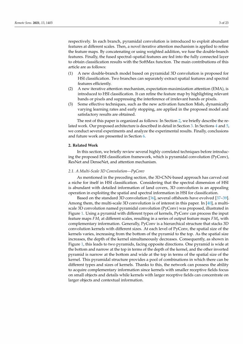
Based on the standard 3D convolution [36], several offshoots have evolved [37–39].Among them, the multi-scale 3D convolution is of interest in this paper. In [40], a multi-scale 3D convolution named pyramidal convolution (PyConv) was proposed, illustrated inFigure 1. Using a pyramid with different types of kernels, PyConv can process the inputfeature maps FMi at different scales, resulting in a series of output feature maps FMo withcomplementary information. Generally, PyConv is a hierarchical structure that stacks 3Dconvolution kernels with different sizes. At each level of PyConv, the spatial size of thekernels varies, increasing from the bottom of the pyramid to the top. As the spatial sizeincreases, the depth of the kernel simultaneously decreases. Consequently, as shown inFigure 1, this leads to two pyramids, facing opposite directions. One pyramid is wide atthe bottom and narrow at the top in terms of the depth of the kernel, and the other invertedpyramid is narrow at the bottom and wide at the top in terms of the spatial size of thekernel. This pyramidal structure provides a pool of combinations in which there can bedifferent types and sizes of kernels. Thanks to this, the network can possess the abilityto acquire complementary information since kernels with smaller receptive fields focuson small objects and details while kernels with larger receptive fields can concentrate onlarger objects and contextual information.

Remote Sens. 2021, 13, 1403 4 of 23Remote Sens. 2021, 13, x FOR PEER REVIEW 4 of 24
Figure 1. Pyramidal convolution (PyConv).
2.2. ResNet and DenseNet
Deep networks can lead to better performance, but optimizing deep networks is very
difficult. To combat this dilemma, ResNet and DenseNet are powerful tools.
Inspired by residual representations in image recognition, ResNet introduces
shortcut connections to the network. As shown in Figure 2(a), 𝐻 denotes hidden layers,
including convolution layers, activation function layers, and batch normalization (BN)
layers. In the original text of ResNet, shortcut connections simply perform identity
mapping, enabling information or gradient to pass directly without travelling through
intermediate layers. To mathematically formalize residual learning, identity mapping by
shortcuts is integrated into a basic block in ResNet, which can be defined as:
𝑥𝑙 = 𝐻𝑙(𝑥𝑙−1) + 𝑥𝑙−1 (1)
Based on ResNet, DenseNet connect all layers directly with each other to ensure
maximum information flow through the network all the time. To maintain the feed-
forward nature, each layer concatenates the outputs of all previous layers as inputs in the
channel dimension and transmits its own feature maps to all subsequent layers. Figure
2(b) illustrates this layout. Accordingly, the input 𝑥𝑙 of 𝑙𝑡ℎ layer can be formulated as:
𝑥𝑙 = 𝐻𝑙([𝑥0, 𝑥1, ⋯ , 𝑥𝑙−1]) (2)
where 𝐻𝑙 refers to a module consists of convolution layers, activation layers, and BN
layers, and [𝑥0, 𝑥1, ⋯ , 𝑥𝑙−1] denotes the concatenation of the feature maps generated by
all preceding layers.
Figure 1. Pyramidal convolution (PyConv).
2.2. ResNet and DenseNet
Deep networks can lead to better performance, but optimizing deep networks is verydifficult. To combat this dilemma, ResNet and DenseNet are powerful tools.
Inspired by residual representations in image recognition, ResNet introduces shortcutconnections to the network. As shown in Figure 2a H, denotes hidden layers, includingconvolution layers, activation function layers, and batch normalization (BN) layers. In theoriginal text of ResNet, shortcut connections simply perform identity mapping, enablinginformation or gradient to pass directly without travelling through intermediate layers. Tomathematically formalize residual learning, identity mapping by shortcuts is integratedinto a basic block in ResNet, which can be defined as:
xl = Hl(xl−1) + xl−1 (1)Remote Sens. 2021, 13, x FOR PEER REVIEW 5 of 24
Figure 2. (a)The core block of residual network (ResNet) and (b) dense convolutional network
(DenseNet).
2.3. Attention Mechanism
Given that the recognition ability of the different bands varies, the same object tends
to show different spectral responses to different bands. Plus, different areas of the data
cube contain different semantic information. Such prior information can facilitate the
competence of the model once when it is fully exploited. The attention mechanism is
exactly the powerful technique that meets the demands. The essence of the attention
mechanism is to obtain a new representation with linear weighting based on the
correlations between objects, which can be interpreted as a method of feature
transformation. To date, the attention mechanism has been successfully applied to various
tasks, such as video classification [41], machine translation [42] and scene segmentation
[43].
Among the diverse attention models, the self-attention [42] is popular, which
computes a weighted summation of location contexts. Non-local [40] first introduced the
self-attention mechanism to computer vision tasks. DANet [34] treated the Non-local
operation as the spatial attention, and further proposed the channel attention, integrating
two branches as an overall framework. 𝐴2net [44] used a dual-attention block to gather
crucial features from entire spatio-temporal spaces into a compact set and then adaptively
distribute them to each position.
However, these methods tend to drive each pixel to capture global information,
resulting in attention maps with high time and space complexity. Motivated by the
success of attention in the above works, EMANet [45] rethought the attention mechanism
from the perspective of the expectation-maximization (EM) algorithm and computed
attention maps in an iterative manner, significantly alleviating the burden of computation.
As shown in Figure 3, a set of bases representing the input feature is initialized first, then
with the EM algorithm, the update of the attention maps is executed in 𝐸 step and the
update of bases is executed in 𝑀 step. Two steps are conducted alternately until
convergence. Such mechanism can be integrated into a unit called Expectation-
Maximization Attention Unit (EMAU), which can be conveniently inserted to CNNs.
Figure 2. (a)The core block of residual network (ResNet) and (b) dense convolutional network(DenseNet).

Remote Sens. 2021, 13, 1403 5 of 23
Based on ResNet, DenseNet connect all layers directly with each other to ensuremaximum information flow through the network all the time. To maintain the feed-forward nature, each layer concatenates the outputs of all previous layers as inputs in thechannel dimension and transmits its own feature maps to all subsequent layers. Figure 2billustrates this layout. Accordingly, the input xl of lth layer can be formulated as:
xl = Hl([x0, x1, · · · , xl−1]) (2)
where Hl refers to a module consists of convolution layers, activation layers, and BNlayers, and [x0, x1, · · · , xl−1] denotes the concatenation of the feature maps generated byall preceding layers.
2.3. Attention Mechanism
Given that the recognition ability of the different bands varies, the same object tendsto show different spectral responses to different bands. Plus, different areas of the datacube contain different semantic information. Such prior information can facilitate thecompetence of the model once when it is fully exploited. The attention mechanism isexactly the powerful technique that meets the demands. The essence of the attentionmechanism is to obtain a new representation with linear weighting based on the correlationsbetween objects, which can be interpreted as a method of feature transformation. To date,the attention mechanism has been successfully applied to various tasks, such as videoclassification [41], machine translation [42] and scene segmentation [43].
Among the diverse attention models, the self-attention [42] is popular, which computesa weighted summation of location contexts. Non-local [40] first introduced the self-attentionmechanism to computer vision tasks. DANet [34] treated the Non-local operation as thespatial attention, and further proposed the channel attention, integrating two branches asan overall framework. A2 net [44] used a dual-attention block to gather crucial featuresfrom entire spatio-temporal spaces into a compact set and then adaptively distribute themto each position.
However, these methods tend to drive each pixel to capture global information,resulting in attention maps with high time and space complexity. Motivated by the successof attention in the above works, EMANet [45] rethought the attention mechanism fromthe perspective of the expectation-maximization (EM) algorithm and computed attentionmaps in an iterative manner, significantly alleviating the burden of computation. As shownin Figure 3, a set of bases representing the input feature is initialized first, then with theEM algorithm, the update of the attention maps is executed in E step and the update ofbases is executed in M step. Two steps are conducted alternately until convergence. Suchmechanism can be integrated into a unit called Expectation-Maximization Attention Unit(EMAU), which can be conveniently inserted to CNNs.
Suppose an input feature map is X ∈ RN×C and the bases are initialized as B ∈ RK×C.In E step, we use bases to generate the attention maps Y ∈ RN×K according to the followingformulations:
ynk =K(xn, βk)
∑Ki=1 K(xn, βi)
(3)
Z = softmax(
XBT)
(4)
where ynk represents the weight of the contribution of the k-th base βk to the n-th pixelxn. Equation (4) is the matrix calculation version of Equation (3), which is the actuallyapplication in the experiment.
In M step, the attention maps are used to update the bases:
βk =∑N
n=1 ynkxn
∑Nn=1 ynk
(5)
Remote Sens. 2021, 13, 1403 6 of 23
where the bases B is the weighted sum of X to keep both in the same representation space,aiming to guarantee the robustness of iterations.
Remote Sens. 2021, 13, x FOR PEER REVIEW 6 of 24
Figure 3. Expectation-maximization (EM) attention operation.
Suppose an input feature map is 𝑋 ∈ 𝑅𝑁×𝐶 and the bases are initialized as ℬ ∈ 𝑅𝐾×𝐶 .
In E step, we use bases to generate the attention maps 𝑌 ∈ 𝑅𝑁×𝐾 according to the
following formulations:
𝑦𝑛𝑘 =K(𝑥𝑛 , 𝛽𝑘)
∑ K(𝑥𝑛 , 𝛽𝑖)𝐾𝑖=1
(3)
Z = softmax(Xℬ𝑇) (4)
where 𝑦𝑛𝑘 represents the weight of the contribution of the 𝑘-th base 𝛽𝑘 to the 𝑛-th pixel
𝑥𝑛. Equation (4) is the matrix calculation version of Equation (3), which is the actually
application in the experiment.
In M step, the attention maps are used to update the bases:
𝛽𝑘 =∑ 𝑦𝑛𝑘
𝑁𝑛=1 𝑥𝑛
∑ 𝑦𝑛𝑘𝑁𝑛=1
(5)
where the bases ℬ is the weighted sum of 𝑋 to keep both in the same representation
space, aiming to guarantee the robustness of iterations.
After two steps are executed alternately for 𝑇 times, ℬ and 𝑌 could converge
approximately, which is guaranteed by the property of the EM algorithm. Experimental
results also demonstrate that the number of iterations 𝑇 is a small constant, i.e.,
expectation-maximization attention can converge quickly. Then, the final ℬ and 𝑌 are
used to reconstruct 𝑋. The new 𝑋, notated as �̃�, can be formulated as:
�̃� = 𝑌ℬ (6)
here �̃� can be deemed as a low-rank version of 𝑋.
3. Methodology
This section is structured as follows. First, we introduce the framework of the
proposed method. Second, two branches respectively focusing on spectral information
and spatial information are described in detail. Third, fusion operations of spectral and
spatial branches are discussed. Finally, several techniques aimed at boosting the network
performance are covered.
3.1. Framework of the Proposed Model
The flowchart in Figure 4 depicts the proposed model for HSI classification.
Generally, it consists of two branches: the spectral branch and the spatial branch.
Moreover, Expectation-Maximization attention modules are incorporated into both
branches to apply attention-based feature refinement. Concatenation or weighted sum are
implemented subsequently to fuse bipartite features. Finally, classification is performed
with the SoftMax function.
Figure 3. Expectation-maximization (EM) attention operation.
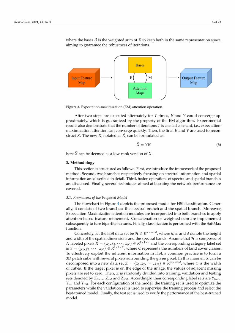
After two steps are executed alternately for T times, B and Y could converge ap-proximately, which is guaranteed by the property of the EM algorithm. Experimentalresults also demonstrate that the number of iterations T is a small constant, i.e., expectation-maximization attention can converge quickly. Then, the final B and Y are used to recon-struct X. The new X, notated as X̃, can be formulated as:
X̃ = YB (6)
here X̃ can be deemed as a low-rank version of X.
3. Methodology
This section is structured as follows. First, we introduce the framework of the proposedmethod. Second, two branches respectively focusing on spectral information and spatialinformation are described in detail. Third, fusion operations of spectral and spatial branchesare discussed. Finally, several techniques aimed at boosting the network performance arecovered.
3.1. Framework of the Proposed Model
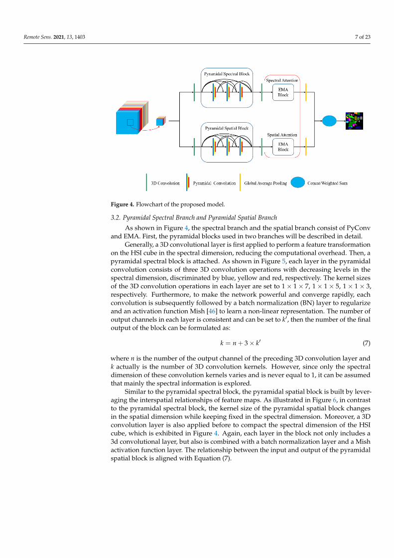
The flowchart in Figure 4 depicts the proposed model for HSI classification. Gener-ally, it consists of two branches: the spectral branch and the spatial branch. Moreover,Expectation-Maximization attention modules are incorporated into both branches to applyattention-based feature refinement. Concatenation or weighted sum are implementedsubsequently to fuse bipartite features. Finally, classification is performed with the SoftMaxfunction.
Concretely, let the HSI data set be H ∈ Rh×w×d, where h, w and d denote the heightand width of the spatial dimensions and the spectral bands. Assume thatH is composed ofN labeled pixels X = {x1, x2, · · · , xN} ∈ R1×1×d and the corresponding category label setis Y = {y1, y2, · · · , xN} ∈ R1×1×C, where C represents the numbers of land cover classes.To effectively exploit the inherent information in HSI, a common practice is to form a3D patch cube with several pixels surrounding the given pixel. In this manner, X can bedecomposed into a new data set Z = {z1, z2, · · · , zN} ∈ Rw×w×d, where w is the widthof cubes. If the target pixel is on the edge of the image, the values of adjacent missingpixels are set to zero. Then, Z is randomly divided into training, validation and testingsets denoted by Ztrain, Zval and Ztest. Accordingly, their corresponding label sets are Ytrain,Yval and Ytest. For each configuration of the model, the training set is used to optimize theparameters while the validation set is used to supervise the training process and select thebest-trained model. Finally, the test set is used to verify the performance of the best-trainedmodel.
Remote Sens. 2021, 13, 1403 7 of 23Remote Sens. 2021, 13, x FOR PEER REVIEW 7 of 24
Figure 4. Flowchart of the proposed model.
Concretely, let the HSI data set be ℋ ∈ 𝑅ℎ×𝑤×𝑑 , where ℎ , 𝑤 and 𝑑 denote the
height and width of the spatial dimensions and the spectral bands. Assume that ℋ is
composed of 𝑁 labeled pixels 𝑋 = {𝑥1, 𝑥2, ⋯ , 𝑥𝑁} ∈ 𝑅1×1×𝑑 and the corresponding
category label set is 𝑌 = {𝑦1, 𝑦2, ⋯ , 𝑥𝑁} ∈ 𝑅1×1×𝐶, where 𝐶 represents the numbers of land
cover classes. To effectively exploit the inherent information in HSI, a common practice is
to form a 3D patch cube with several pixels surrounding the given pixel. In this manner,
𝑋 can be decomposed into a new data set 𝑍 = {𝑧1, 𝑧2, ⋯ , 𝑧𝑁} ∈ 𝑅𝑤×𝑤×𝑑, where 𝑤 is the
width of cubes. If the target pixel is on the edge of the image, the values of adjacent
missing pixels are set to zero. Then, 𝑍 is randomly divided into training, validation and
testing sets denoted by 𝑍𝑡𝑟𝑎𝑖𝑛, 𝑍𝑣𝑎𝑙 and 𝑍𝑡𝑒𝑠𝑡. Accordingly, their corresponding label sets
are 𝑌𝑡𝑟𝑎𝑖𝑛, 𝑌𝑣𝑎𝑙 and 𝑌𝑡𝑒𝑠𝑡 . For each configuration of the model, the training set is used to
optimize the parameters while the validation set is used to supervise the training process
and select the best-trained model. Finally, the test set is used to verify the performance of
the best-trained model.
3.2. Pyramidal Spectral Branch and Pyramidal Spatial Branch
As shown in Figure 4, the spectral branch and the spatial branch consist of PyConv
and EMA. First, the pyramidal blocks used in two branches will be described in detail.
Generally, a 3D convolutional layer is first applied to perform a feature
transformation on the HSI cube in the spectral dimension, reducing the computational
overhead. Then, a pyramidal spectral block is attached. As shown in Figure 5, each layer
in the pyramidal convolution consists of three 3D convolution operations with decreasing
levels in the spectral dimension, discriminated by blue, yellow and red, respectively. The
kernel sizes of the 3D convolution operations in each layer are set to 1 × 1 × 7, 1 × 1 × 5,
1 × 1 × 3, respectively. Furthermore, to make the network powerful and converge rapidly,
each convolution is subsequently followed by a batch normalization (BN) layer to
regularize and an activation function Mish [46] to learn a non-linear representation. The
number of output channels in each layer is consistent and can be set to 𝑘′ , then the
number of the final output of the block can be formulated as:
𝑘 = 𝑛 + 3 × 𝑘′ (7)
where 𝑛 is the number of the output channel of the preceding 3D convolution layer and
𝑘 actually is the number of 3D convolution kernels. However, since only the spectral
dimension of these convolution kernels varies and is never equal to 1, it can be assumed
that mainly the spectral information is explored.
Figure 4. Flowchart of the proposed model.
3.2. Pyramidal Spectral Branch and Pyramidal Spatial Branch
As shown in Figure 4, the spectral branch and the spatial branch consist of PyConvand EMA. First, the pyramidal blocks used in two branches will be described in detail.
Generally, a 3D convolutional layer is first applied to perform a feature transformationon the HSI cube in the spectral dimension, reducing the computational overhead. Then, apyramidal spectral block is attached. As shown in Figure 5, each layer in the pyramidalconvolution consists of three 3D convolution operations with decreasing levels in thespectral dimension, discriminated by blue, yellow and red, respectively. The kernel sizesof the 3D convolution operations in each layer are set to 1× 1× 7, 1× 1× 5, 1× 1× 3,respectively. Furthermore, to make the network powerful and converge rapidly, eachconvolution is subsequently followed by a batch normalization (BN) layer to regularizeand an activation function Mish [46] to learn a non-linear representation. The number ofoutput channels in each layer is consistent and can be set to k′, then the number of the finaloutput of the block can be formulated as:
k = n + 3× k′ (7)
where n is the number of the output channel of the preceding 3D convolution layer andk actually is the number of 3D convolution kernels. However, since only the spectraldimension of these convolution kernels varies and is never equal to 1, it can be assumedthat mainly the spectral information is explored.
Similar to the pyramidal spectral block, the pyramidal spatial block is built by lever-aging the interspatial relationships of feature maps. As illustrated in Figure 6, in contrastto the pyramidal spectral block, the kernel size of the pyramidal spatial block changesin the spatial dimension while keeping fixed in the spectral dimension. Moreover, a 3Dconvolution layer is also applied before to compact the spectral dimension of the HSIcube, which is exhibited in Figure 4. Again, each layer in the block not only includes a3d convolutional layer, but also is combined with a batch normalization layer and a Mishactivation function layer. The relationship between the input and output of the pyramidalspatial block is aligned with Equation (7).

Remote Sens. 2021, 13, 1403 8 of 23Remote Sens. 2021, 13, x FOR PEER REVIEW 8 of 24
Figure 5. Pyramidal spectral block.
Similar to the pyramidal spectral block, the pyramidal spatial block is built by
leveraging the interspatial relationships of feature maps. As illustrated in Figure 6, in
contrast to the pyramidal spectral block, the kernel size of the pyramidal spatial block
changes in the spatial dimension while keeping fixed in the spectral dimension. Moreover,
a 3D convolution layer is also applied before to compact the spectral dimension of the HSI
cube, which is exhibited in Figure 4. Again, each layer in the block not only includes a 3d
convolutional layer, but also is combined with a batch normalization layer and a Mish
activation function layer. The relationship between the input and output of the pyramidal
spatial block is aligned with Equation (7).
Figure 6. Pyramidal spatial block.
3.3. Expectation-Maximization Attention Block
After attaching the pyramidal spectral or spatial block, a 3D convolutional layer is
needed to ‘resize’ intermediate feature maps for subsequent input to the EMA block. Then,
the EMA block follows to refine feature maps. In view of the fact that for the same object,
the spectral response may vary dramatically on different bands. In addition, different
positions of the extracted feature maps can provide different semantic information for HSI
classification. The performance for HSI classification can be improved if such prior
information can be properly taken into account. Therefore, the EMA block is introduced.
Two EMA blocks located in the spectral and spatial branches are designed with a similar
structure. The EMA block located in the spectral branch iterates the attention map along
the spectral dimension (denoted as spectral attention), while the EMA block located in the
Figure 5. Pyramidal spectral block.
Remote Sens. 2021, 13, x FOR PEER REVIEW 8 of 24
Figure 5. Pyramidal spectral block.
Similar to the pyramidal spectral block, the pyramidal spatial block is built by
leveraging the interspatial relationships of feature maps. As illustrated in Figure 6, in
contrast to the pyramidal spectral block, the kernel size of the pyramidal spatial block
changes in the spatial dimension while keeping fixed in the spectral dimension. Moreover,
a 3D convolution layer is also applied before to compact the spectral dimension of the HSI
cube, which is exhibited in Figure 4. Again, each layer in the block not only includes a 3d
convolutional layer, but also is combined with a batch normalization layer and a Mish
activation function layer. The relationship between the input and output of the pyramidal
spatial block is aligned with Equation (7).
Figure 6. Pyramidal spatial block.
3.3. Expectation-Maximization Attention Block
After attaching the pyramidal spectral or spatial block, a 3D convolutional layer is
needed to ‘resize’ intermediate feature maps for subsequent input to the EMA block. Then,
the EMA block follows to refine feature maps. In view of the fact that for the same object,
the spectral response may vary dramatically on different bands. In addition, different
positions of the extracted feature maps can provide different semantic information for HSI
classification. The performance for HSI classification can be improved if such prior
information can be properly taken into account. Therefore, the EMA block is introduced.
Two EMA blocks located in the spectral and spatial branches are designed with a similar
structure. The EMA block located in the spectral branch iterates the attention map along
the spectral dimension (denoted as spectral attention), while the EMA block located in the
Figure 6. Pyramidal spatial block.
3.3. Expectation-Maximization Attention Block
After attaching the pyramidal spectral or spatial block, a 3D convolutional layer isneeded to ‘resize’ intermediate feature maps for subsequent input to the EMA block. Then,the EMA block follows to refine feature maps. In view of the fact that for the same object,the spectral response may vary dramatically on different bands. In addition, differentpositions of the extracted feature maps can provide different semantic information forHSI classification. The performance for HSI classification can be improved if such priorinformation can be properly taken into account. Therefore, the EMA block is introduced.Two EMA blocks located in the spectral and spatial branches are designed with a similarstructure. The EMA block located in the spectral branch iterates the attention map alongthe spectral dimension (denoted as spectral attention), while the EMA block located in thespatial branch iterates the attention map along the spatial dimension (denoted as spatialattention).
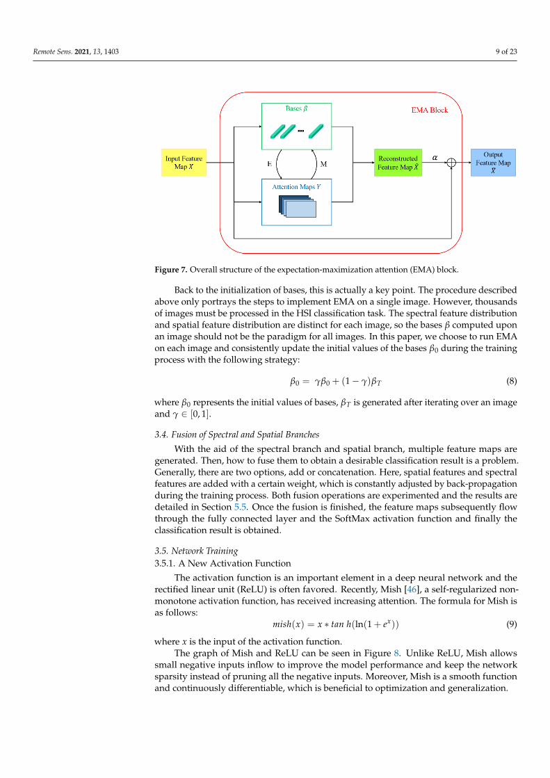
As shown in Figure 7, given an intermediate feature map X as input, a compact baseset is initialized with Kaiming’s initialization [47]. Then, attention maps can be generatedin E step and the base set can be updated in M step, as described in Section 2.3. After a fewiterations, with the converged bases and attention maps, a new refined feature map X̂ canbe obtained. Instead of outputting X̂ directly, a small factor α is adopted to equilibrate Xwith X̂. Multiplying X̂ by α and then adding it to X, the final output X is generated. Thisoperation facilitates the stability of the training and empirical performance validates thepotency.
Remote Sens. 2021, 13, 1403 9 of 23
Remote Sens. 2021, 13, x FOR PEER REVIEW 9 of 24
spatial branch iterates the attention map along the spatial dimension (denoted as spatial
attention).
As shown in Figure 7, given an intermediate feature map 𝑋 as input, a compact base
set is initialized with Kaiming’s initialization [47]. Then, attention maps can be generated
in 𝐸 step and the base set can be updated in 𝑀 step, as described in Section 2.3. After a
few iterations, with the converged bases and attention maps, a new refined feature map
�̂� can be obtained. Instead of outputting �̂� directly, a small factor 𝛼 is adopted to
equilibrate 𝑋 with �̂�. Multiplying �̂� by 𝛼 and then adding it to 𝑋, the final output �̅� is
generated. This operation facilitates the stability of the training and empirical
performance validates the potency.
Back to the initialization of bases, this is actually a key point. The procedure described
above only portrays the steps to implement EMA on a single image. However, thousands
of images must be processed in the HSI classification task. The spectral feature
distribution and spatial feature distribution are distinct for each image, so the bases 𝛽
computed upon an image should not be the paradigm for all images. In this paper, we
choose to run EMA on each image and consistently update the initial values of the bases
𝛽0 during the training process with the following strategy:
𝛽0 = 𝛾𝛽0 + (1 − 𝛾)𝛽𝑇 (6)
where 𝛽0 represents the initial values of bases, 𝛽𝑇 is generated after iterating over an
image and 𝛾 ∈ [0,1].
Figure 7. Overall structure of the expectation-maximization attention (EMA) block.
3.4. Fusion of Spectral and Spatial Branches
With the aid of the spectral branch and spatial branch, multiple feature maps are
generated. Then, how to fuse them to obtain a desirable classification result is a problem.
Generally, there are two options, add or concatenation. Here, spatial features and spectral
features are added with a certain weight, which is constantly adjusted by back-
propagation during the training process. Both fusion operations are experimented and the
results are detailed in Section 5.5. Once the fusion is finished, the feature maps
subsequently flow through the fully connected layer and the SoftMax activation function
and finally the classification result is obtained.
3.5. Network Training
3.5.1. A New Activation Function
The activation function is an important element in a deep neural network and the
rectified linear unit (ReLU) is often favored. Recently, Mish [46], a self-regularized non-
Figure 7. Overall structure of the expectation-maximization attention (EMA) block.
Back to the initialization of bases, this is actually a key point. The procedure describedabove only portrays the steps to implement EMA on a single image. However, thousandsof images must be processed in the HSI classification task. The spectral feature distributionand spatial feature distribution are distinct for each image, so the bases β computed uponan image should not be the paradigm for all images. In this paper, we choose to run EMAon each image and consistently update the initial values of the bases β0 during the trainingprocess with the following strategy:
β0 = γβ0 + (1− γ)βT (8)
where β0 represents the initial values of bases, βT is generated after iterating over an imageand γ ∈ [0, 1].
3.4. Fusion of Spectral and Spatial Branches
With the aid of the spectral branch and spatial branch, multiple feature maps aregenerated. Then, how to fuse them to obtain a desirable classification result is a problem.Generally, there are two options, add or concatenation. Here, spatial features and spectralfeatures are added with a certain weight, which is constantly adjusted by back-propagationduring the training process. Both fusion operations are experimented and the results aredetailed in Section 5.5. Once the fusion is finished, the feature maps subsequently flowthrough the fully connected layer and the SoftMax activation function and finally theclassification result is obtained.
3.5. Network Training3.5.1. A New Activation Function
The activation function is an important element in a deep neural network and therectified linear unit (ReLU) is often favored. Recently, Mish [46], a self-regularized non-monotone activation function, has received increasing attention. The formula for Mish isas follows:
mish(x) = x ∗ tan h(ln(1 + ex)) (9)
where x is the input of the activation function.The graph of Mish and ReLU can be seen in Figure 8. Unlike ReLU, Mish allows
small negative inputs inflow to improve the model performance and keep the networksparsity instead of pruning all the negative inputs. Moreover, Mish is a smooth functionand continuously differentiable, which is beneficial to optimization and generalization.

Remote Sens. 2021, 13, 1403 10 of 23
Remote Sens. 2021, 13, x FOR PEER REVIEW 10 of 24
monotone activation function, has received increasing attention. The formula for Mish is
as follows:
𝑚𝑖𝑠ℎ(𝑥) = 𝑥 ∗ 𝑡𝑎𝑛 ℎ(𝑙𝑛(1 + 𝑒𝑥)) (7)
where 𝑥 is the input of the activation function.
Figure 8. The graph of Mish and ReLU.
The graph of Mish and ReLU can be seen in Figure 8. Unlike ReLU, Mish allows small
negative inputs inflow to improve the model performance and keep the network sparsity
instead of pruning all the negative inputs. Moreover, Mish is a smooth function and
continuously differentiable, which is beneficial to optimization and generalization.
3.5.2. Other Training Tricks
To mitigate the overfitting problem, dropout [48] is a typical strategy. Given a
percentage 𝑝, which is selected as 0.5 in the proposed model, the network would drop
out hidden or visible units temporarily. In the case of stochastic gradient descent, a new
network is trained in each mini-batch due to the property of random dropping. Moreover,
dropout can make only a few units in the network possess high activation ability, which
is conducive to the sparsity of the network. In our framework, a dropout layer is applied
after the EMA block.
In addition, the early stopping strategy, and the dynamic learning rate adjustment
method are also adopted to accelerate the network training. Specifically, early stopping
means stopping the training if the loss function no longer decreases in a couple of training
epochs (which is 20 in our method). Dynamic learning rate means that we adjust the
learning rate during the training process to avoid the model trapped in a local optimum.
Herein, we use the cosine annealing [49] strategy, which is formulated as follows:
𝜂t = 𝜂𝑚𝑖𝑛𝑖 +
1
2(𝜂𝑚𝑎𝑥
𝑖 − 𝜂𝑚𝑖𝑛𝑖 ) (1 + cos (
𝑇𝑐𝑢𝑟
𝑇𝑖
𝜋)) (8)
where 𝜂t is the learning rate for the 𝑖-th run while 𝜂𝑚𝑖𝑛𝑖 and 𝜂𝑚𝑎𝑥
𝑖 are ranges for the
learning rate. 𝑇𝑐𝑢𝑟 denotes how many epochs have been executed since the last restart
and 𝑇𝑖 represents the number of epochs in one restart cycle.
4. Experiment
4.1. Datasets Description
Figure 8. The graph of Mish and ReLU.
3.5.2. Other Training Tricks
To mitigate the overfitting problem, dropout [48] is a typical strategy. Given a percent-age p, which is selected as 0.5 in the proposed model, the network would drop out hiddenor visible units temporarily. In the case of stochastic gradient descent, a new network istrained in each mini-batch due to the property of random dropping. Moreover, dropout canmake only a few units in the network possess high activation ability, which is conducive tothe sparsity of the network. In our framework, a dropout layer is applied after the EMAblock.
In addition, the early stopping strategy, and the dynamic learning rate adjustmentmethod are also adopted to accelerate the network training. Specifically, early stoppingmeans stopping the training if the loss function no longer decreases in a couple of trainingepochs (which is 20 in our method). Dynamic learning rate means that we adjust thelearning rate during the training process to avoid the model trapped in a local optimum.Herein, we use the cosine annealing [49] strategy, which is formulated as follows:
ηt = ηimin +
12
(ηi
max − ηimin
)(1 + cos
(Tcur
Tiπ
))(10)
where ηt is the learning rate for the i-th run while ηimin and ηi
max are ranges for the learningrate. Tcur denotes how many epochs have been executed since the last restart and Tirepresents the number of epochs in one restart cycle.
4. Experiment4.1. Datasets Description
In the experiments, four publicly available datasets, the Pavia University (UP)dataset,the Indian Pines (IP) dataset, the Salinas Valley (SV) dataset, and the Botswana dataset (BS),are applied to conduct a series of experiments.
Pavia University (UP): captured by the reflective optics imaging spectrometer (ROSIS-3)sensor at the University of Pavia, northern Italy, the Pavia University dataset is comprisedof 103 bands with spatial resolution of 1.3 mpp in the wavelength ranging from 0.43 µm to0.86 µm. The spatial size is 610× 340 pixels and 9 land cover classes are involved.
Indian Pines (IP): captured by the Airborne Visible/Infrared Imaging Spectrometer(AVIRIS) sensor in the north-western Indiana, the Indian Pines dataset is comprised of
Remote Sens. 2021, 13, 1403 11 of 23
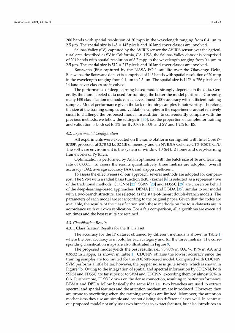
200 bands with spatial resolution of 20 mpp in the wavelength ranging from 0.4 µm to2.5 µm. The spatial size is 145× 145 pixels and 16 land cover classes are involved.
Salinas Valley (SV): captured by the AVIRIS sensor the AVIRIS sensor over the agricul-tural area described as SV in California, CA, USA, the Salinas Valley dataset is comprisedof 204 bands with spatial resolution of 3.7 mpp in the wavelength ranging from 0.4 µm to2.5 µm. The spatial size is 512× 217 pixels and 16 land cover classes are involved.
Botswana (BS): captured by the NASA EO-1 satellite over the Okavango Delta,Botswana, the Botswana dataset is comprised of 145 bands with spatial resolution of 20 mppin the wavelength ranging from 0.4 µm to 2.5 µm. The spatial size is 1476× 256 pixels and14 land cover classes are involved.
The performance of deep-learning-based models strongly depends on the data. Gen-erally, the more labeled data used for training, the better the model performs. Currently,many HSI classification methods can achieve almost 100% accuracy with sufficient trainingsamples. Model performance given the lack of training samples is noteworthy. Therefore,the size of the training samples and validation samples in the experiments are set relativelysmall to challenge the proposed model. In addition, to conveniently compare with theprevious methods, we follow the settings in [35], i.e., the proportion of samples for trainingand validation is both set to 3% for IP, 0.5% for UP and SV and 1.2% for BS.
4.2. Experimental Configuration
All experiments were executed on the same platform configured with Intel Core i7-8700K processor at 3.70 GHz, 32 GB of memory and an NVIDIA GeForce GTX 1080Ti GPU.The software environment is the system of window 10 (64 bit) home and deep-learningframeworks of PyTorch.
Optimization is performed by Adam optimizer with the batch size of 16 and learningrate of 0.0005. To assess the results quantitatively, three metrics are adopted: overallaccuracy (OA), average accuracy (AA), and Kappa coefficient.
To assess the effectiveness of our approach, several methods are adopted for compari-son. The SVM with a radial basis function (RBF) kernel [6] is selected as a representativeof the traditional methods. CDCNN [22], SSRN [28] and FDSSC [29] are chosen on behalfof the deep-learning-based approaches. DBMA [33] and DBDA [35], similar to our modelwith a two-branch structure, are selected as the state-of-the-art double-branch models. Theparameters of each model are set according to the original paper. Given that the codes areavailable, the results of the classification with these methods on the four datasets are inaccordance with our own replication. For a fair comparison, all algorithms are executedten times and the best results are retained.
4.3. Classification Results4.3.1. Classification Results for the IP Dataset
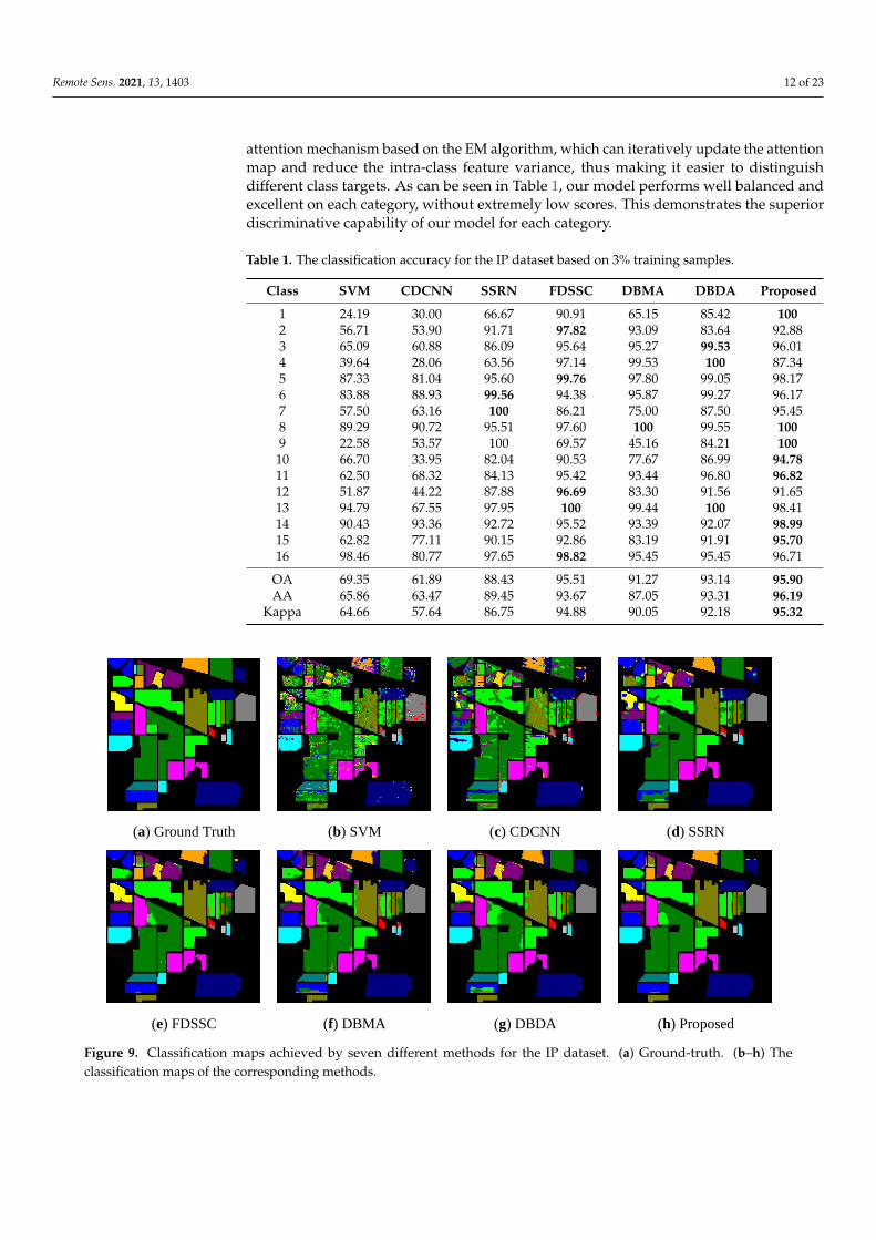
The accuracy for the IP dataset obtained by different methods is shown in Table 1,where the best accuracy is in bold for each category and for the three metrics. The corre-sponding classification maps are also illustrated in Figure 9.
The proposed model yields the best results, i.e., 95.90% in OA, 96.19% in AA and0.9532 in Kappa, as shown in Table 1. CDCNN obtains the lowest accuracy since thetraining samples are too limited for the 2DCNN-based model. Compared with CDCNN,SVM performs a little better; however, the pepper noise is quite severe, which is shown inFigure 9b. Owing to the integration of spatial and spectral information by 3DCNN, bothSSRN and FDSSC are far superior to SVM and CDCNN, exceeding them by almost 20% inOA. Furthermore, FDSSC draws on the dense connection, resulting in better performance.DBMA and DBDA follow basically the same idea i.e., two branches are used to extractspectral and spatial features and the attention mechanism are introduced. However, theyare prone to overfitting when the training samples are limited. Moreover, the attentionmechanisms they use are simple and cannot distinguish different classes well. In contrast,our proposed model not only uses two branches to extract features, but also introduces an
Remote Sens. 2021, 13, 1403 12 of 23
attention mechanism based on the EM algorithm, which can iteratively update the attentionmap and reduce the intra-class feature variance, thus making it easier to distinguishdifferent class targets. As can be seen in Table 1, our model performs well balanced andexcellent on each category, without extremely low scores. This demonstrates the superiordiscriminative capability of our model for each category.
Table 1. The classification accuracy for the IP dataset based on 3% training samples.
Class SVM CDCNN SSRN FDSSC DBMA DBDA Proposed
1 24.19 30.00 66.67 90.91 65.15 85.42 1002 56.71 53.90 91.71 97.82 93.09 83.64 92.883 65.09 60.88 86.09 95.64 95.27 99.53 96.014 39.64 28.06 63.56 97.14 99.53 100 87.345 87.33 81.04 95.60 99.76 97.80 99.05 98.176 83.88 88.93 99.56 94.38 95.87 99.27 96.177 57.50 63.16 100 86.21 75.00 87.50 95.458 89.29 90.72 95.51 97.60 100 99.55 1009 22.58 53.57 100 69.57 45.16 84.21 100
10 66.70 33.95 82.04 90.53 77.67 86.99 94.7811 62.50 68.32 84.13 95.42 93.44 96.80 96.8212 51.87 44.22 87.88 96.69 83.30 91.56 91.6513 94.79 67.55 97.95 100 99.44 100 98.4114 90.43 93.36 92.72 95.52 93.39 92.07 98.9915 62.82 77.11 90.15 92.86 83.19 91.91 95.7016 98.46 80.77 97.65 98.82 95.45 95.45 96.71
OA 69.35 61.89 88.43 95.51 91.27 93.14 95.90AA 65.86 63.47 89.45 93.67 87.05 93.31 96.19
Kappa 64.66 57.64 86.75 94.88 90.05 92.18 95.32
Remote Sens. 2021, 13, x FOR PEER REVIEW 12 of 24
The accuracy for the IP dataset obtained by different methods is shown in Table 1,
where the best accuracy is in bold for each category and for the three metrics. The
corresponding classification maps are also illustrated in Figure 9.
Table 1. The classification accuracy for the IP dataset based on 3% training samples.
Class SVM CDCNN SSRN FDSSC DBMA DBDA Proposed
1 24.19 30.00 66.67 90.91 65.15 85.42 100
2 56.71 53.90 91.71 97.82 93.09 83.64 92.88
3 65.09 60.88 86.09 95.64 95.27 99.53 96.01
4 39.64 28.06 63.56 97.14 99.53 100 87.34
5 87.33 81.04 95.60 99.76 97.80 99.05 98.17
6 83.88 88.93 99.56 94.38 95.87 99.27 96.17
7 57.50 63.16 100 86.21 75.00 87.50 95.45
8 89.29 90.72 95.51 97.60 100 99.55 100
9 22.58 53.57 100 69.57 45.16 84.21 100
10 66.70 33.95 82.04 90.53 77.67 86.99 94.78
11 62.50 68.32 84.13 95.42 93.44 96.80 96.82
12 51.87 44.22 87.88 96.69 83.30 91.56 91.65
13 94.79 67.55 97.95 100 99.44 100 98.41
14 90.43 93.36 92.72 95.52 93.39 92.07 98.99
15 62.82 77.11 90.15 92.86 83.19 91.91 95.70
16 98.46 80.77 97.65 98.82 95.45 95.45 96.71
OA 69.35 61.89 88.43 95.51 91.27 93.14 95.90
AA 65.86 63.47 89.45 93.67 87.05 93.31 96.19
Kappa 64.66 57.64 86.75 94.88 90.05 92.18 95.32
(a) Ground Truth
(b) SVM
(c) CDCNN
(d) SSRN
(e) FDSSC
(f) DBMA
(g) DBDA
(h) Proposed
Figure 9. Classification maps achieved by seven different methods for the IP dataset. (a) Ground-truth. (b–h) The classification
maps of the corresponding methods.
The proposed model yields the best results, i.e., 95.90% in OA, 96.19% in AA and
0.9532 in Kappa, as shown in Table 1. CDCNN obtains the lowest accuracy since the
training samples are too limited for the 2DCNN-based model. Compared with CDCNN,
SVM performs a little better; however, the pepper noise is quite severe, which is shown in
Figure 9b. Owing to the integration of spatial and spectral information by 3DCNN, both
SSRN and FDSSC are far superior to SVM and CDCNN, exceeding them by almost 20%
in OA. Furthermore, FDSSC draws on the dense connection, resulting in better
performance. DBMA and DBDA follow basically the same idea i.e., two branches are used
Figure 9. Classification maps achieved by seven different methods for the IP dataset. (a) Ground-truth. (b–h) Theclassification maps of the corresponding methods.

Remote Sens. 2021, 13, 1403 13 of 23
4.3.2. Classification Results for the UP Dataset
The accuracy for the UP dataset obtained by different methods is shown in Table 2,where the best accuracy is in bold for each category and for the three metrics. The corre-sponding classification maps are also illustrated in Figure 10.
Table 2. The classification accuracy for the UP dataset based on 0.5% training samples.
Class SVM CDCNN SSRN FDSSC DBMA DBDA Proposed
1 80.27 87.17 99.35 95.79 90.10 94.43 93.782 86.95 93.59 96.14 97.46 98.52 98.52 99.213 71.74 43.80 95.99 99.67 74.93 98.86 99.724 96.45 86.71 99.56 99.81 95.10 98.46 97.815 90.85 98.67 100 99.63 99.70 99.55 99.926 77.03 83.76 96.08 97.57 97.93 97.90 99.157 69.71 90.17 73.41 100 98.35 97.61 1008 67.31 67.51 79.25 79.27 84.75 83.57 91.529 99.89 97.18 100 99.25 98.82 99.45 99.57
OA 83.08 87.00 94.23 95.65 94.52 96.31 97.60AA 82.24 83.17 93.31 96.49 93.13 96.48 97.85
Kappa 77.07 82.71 92.31 94.19 92.72 95.08 96.82Remote Sens. 2021, 13, x FOR PEER REVIEW 14 of 24
(a) Ground Truth (b) SVM (c) CDCNN (d) SSRN
(e) FDSSC (f) DBMA (g) DBDA (h) Proposed
Figure 10. Classification maps achieved by seven different methods for the UP dataset. (a) Ground-truth. (b–h) The classification
maps of the corresponding methods.
4.3.3. Classification Results for the SV Dataset
The accuracy for the SV dataset obtained by different methods is shown in Table 3,
where the best accuracy is in bold for each category and for the three metrics. The
corresponding classification maps are also illustrated in Figure 11.
Again, the proposed model obtains the best results with 98.33% OA, 98.91% AA, and
0.9814 Kappa. On the class 15, none of the methods achieves over 90% accuracy except
ours. This can be observed in Figure 11. If we concentrate on the yellow area and the gray
area in the upper left corner of classification maps, it can be found that these two areas
interfere with each other terribly in all the models except ours.
Figure 10. Classification maps achieved by seven different methods for the UP dataset. (a) Ground-truth. (b–h) Theclassification maps of the corresponding methods.
Remote Sens. 2021, 13, 1403 14 of 23
As shown in Table 2, our method achieves the best results on the three metrics. Inparticular, the average improvement over the second-best model, DBDA, is +1.29%, +1.37%,1.74% for OA, AA, and Kappa metrics, respectively. Specifically, for each class, the bestresults are obtained by our method in 5 out of 9 classes. In addition, it is worth noting thatin class 8, which is the most difficult to classify, only our model exceeds 90% in classificationaccuracy. Class 8 is represented by the dark gray line in Figure 10a, which is too slenderfor models to capture. Please note that only DBMA, DBDA and our method achieve theaccuracy over 80 % on category 8. This illustrates the advantage of the attention mechanismin capturing fine features. Moreover, the accuracy of our method exceeds 90%, indicatingthat the attention mechanism adopted by our model stands out.
4.3.3. Classification Results for the SV Dataset
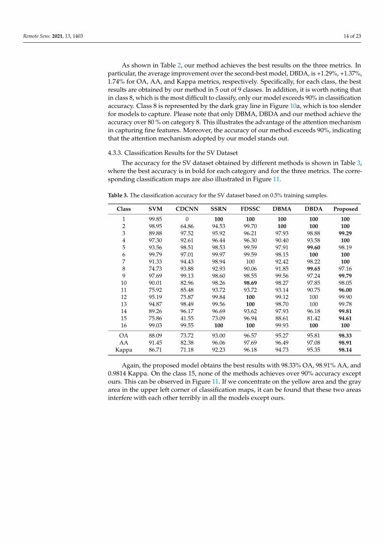
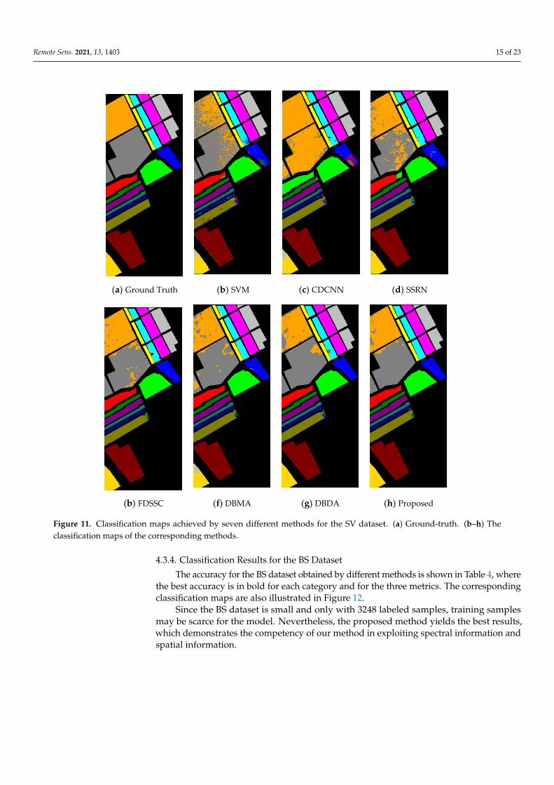
The accuracy for the SV dataset obtained by different methods is shown in Table 3,where the best accuracy is in bold for each category and for the three metrics. The corre-sponding classification maps are also illustrated in Figure 11.
Table 3. The classification accuracy for the SV dataset based on 0.5% training samples.
Class SVM CDCNN SSRN FDSSC DBMA DBDA Proposed
1 99.85 0 100 100 100 100 1002 98.95 64.86 94.53 99.70 100 100 1003 89.88 97.52 95.92 96.21 97.93 98.88 99.294 97.30 92.61 96.44 96.30 90.40 93.58 1005 93.56 98.51 98.53 99.59 97.91 99.60 98.196 99.79 97.01 99.97 99.59 98.15 100 1007 91.33 94.43 98.94 100 92.42 98.22 1008 74.73 93.88 92.93 90.06 91.85 99.65 97.169 97.69 99.13 98.60 98.55 99.56 97.24 99.79
10 90.01 82.96 98.26 98.69 98.27 97.85 98.0511 75.92 85.48 93.72 93.72 93.14 90.75 96.0012 95.19 75.87 99.84 100 99.12 100 99.9013 94.87 98.49 99.56 100 98.70 100 99.7814 89.26 96.17 96.69 93.62 97.93 96.18 99.8115 75.86 41.55 73.09 96.94 88.61 81.42 94.6116 99.03 99.55 100 100 99.93 100 100
OA 88.09 73.72 93.00 96.57 95.27 95.81 98.33AA 91.45 82.38 96.06 97.69 96.49 97.08 98.91
Kappa 86.71 71.18 92.23 96.18 94.73 95.35 98.14
Again, the proposed model obtains the best results with 98.33% OA, 98.91% AA, and0.9814 Kappa. On the class 15, none of the methods achieves over 90% accuracy exceptours. This can be observed in Figure 11. If we concentrate on the yellow area and the grayarea in the upper left corner of classification maps, it can be found that these two areasinterfere with each other terribly in all the models except ours.
Remote Sens. 2021, 13, 1403 15 of 23
Remote Sens. 2021, 13, x FOR PEER REVIEW 15 of 24
Table 3. The classification accuracy for the SV dataset based on 0.5% training samples.
Class SVM CDCNN SSRN FDSSC DBMA DBDA Proposed
1 99.85 0 100 100 100 100 100
2 98.95 64.86 94.53 99.70 100 100 100
3 89.88 97.52 95.92 96.21 97.93 98.88 99.29
4 97.30 92.61 96.44 96.30 90.40 93.58 100
5 93.56 98.51 98.53 99.59 97.91 99.60 98.19
6 99.79 97.01 99.97 99.59 98.15 100 100
7 91.33 94.43 98.94 100 92.42 98.22 100
8 74.73 93.88 92.93 90.06 91.85 99.65 97.16
9 97.69 99.13 98.60 98.55 99.56 97.24 99.79
10 90.01 82.96 98.26 98.69 98.27 97.85 98.05
11 75.92 85.48 93.72 93.72 93.14 90.75 96.00
12 95.19 75.87 99.84 100 99.12 100 99.90
13 94.87 98.49 99.56 100 98.70 100 99.78
14 89.26 96.17 96.69 93.62 97.93 96.18 99.81
15 75.86 41.55 73.09 96.94 88.61 81.42 94.61
16 99.03 99.55 100 100 99.93 100 100
OA 88.09 73.72 93.00 96.57 95.27 95.81 98.33
AA 91.45 82.38 96.06 97.69 96.49 97.08 98.91
Kappa 86.71 71.18 92.23 96.18 94.73 95.35 98.14
(a) Ground Truth (b) SVM (c) CDCNN (d) SSRN
Remote Sens. 2021, 13, x FOR PEER REVIEW 16 of 24
(b) FDSSC (f) DBMA (g) DBDA (h) Proposed
Figure 11. Classification maps achieved by seven different methods for the SV dataset. (a) Ground-truth. (b–h) The classification
maps of the corresponding methods.
4.3.4. Classification Results for the BS Dataset
The accuracy for the BS dataset obtained by different methods is shown in Table 4,
where the best accuracy is in bold for each category and for the three metrics. The
corresponding classification maps are also illustrated in Figure 12.
Since the BS dataset is small and only with 3248 labeled samples, training samples
may be scarce for the model. Nevertheless, the proposed method yields the best results,
which demonstrates the competency of our method in exploiting spectral information and
spatial information.
Table 4. The classification accuracy for the BS dataset based on 1.2% training samples.
Class SVM CDCNN SSRN FDSSC DBMA DBDA Proposed
1 100 91.96 99.62 97.41 98.13 97.72 99.62
2 70.71 80.20 100 74.24 89.91 98.99 100
3 84.11 90.50 98.68 100 100 100 100
4 69.96 96.97 95.87 86.83 91.63 92.95 91.67
5 82.63 72.40 83.92 85.92 94.59 96.97 87.46
6 65.71 65.51 69.25 92.78 77.92 85.62 100
7 78.78 71.65 100 100 86.64 87.54 100
8 65.88 90.00 97.51 92.45 100 100 100
9 75.19 77.74 92.11 84.05 95.24 100 99.34
10 69.82 90.95 83.99 86.83 83.56 86.52 98.78
11 95.50 83.90 97.34 100 99.32 100 100
12 93.10 88.24 100 86.70 99.44 100 100
13 76.25 71.51 100 100 100 100 100
14 90.41 68.86 100 100 100 100 100
OA 78.63 79.84 92.86 92.00 93.11 95.35 98.10
AA 79.57 81.46 94.16 91.94 94.03 96.17 98.35
Kappa 76.88 78.13 92.26 91.34 92.53 94.97 97.94
Figure 11. Classification maps achieved by seven different methods for the SV dataset. (a) Ground-truth. (b–h) Theclassification maps of the corresponding methods.
4.3.4. Classification Results for the BS Dataset
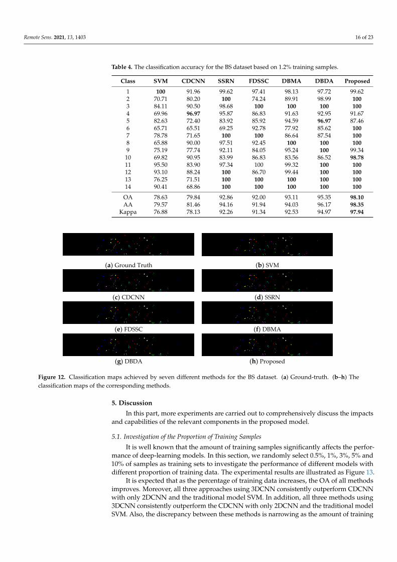
The accuracy for the BS dataset obtained by different methods is shown in Table 4, wherethe best accuracy is in bold for each category and for the three metrics. The correspondingclassification maps are also illustrated in Figure 12.
Since the BS dataset is small and only with 3248 labeled samples, training samplesmay be scarce for the model. Nevertheless, the proposed method yields the best results,which demonstrates the competency of our method in exploiting spectral information andspatial information.
Remote Sens. 2021, 13, 1403 16 of 23
Table 4. The classification accuracy for the BS dataset based on 1.2% training samples.
Class SVM CDCNN SSRN FDSSC DBMA DBDA Proposed
1 100 91.96 99.62 97.41 98.13 97.72 99.622 70.71 80.20 100 74.24 89.91 98.99 1003 84.11 90.50 98.68 100 100 100 1004 69.96 96.97 95.87 86.83 91.63 92.95 91.675 82.63 72.40 83.92 85.92 94.59 96.97 87.466 65.71 65.51 69.25 92.78 77.92 85.62 1007 78.78 71.65 100 100 86.64 87.54 1008 65.88 90.00 97.51 92.45 100 100 1009 75.19 77.74 92.11 84.05 95.24 100 99.34
10 69.82 90.95 83.99 86.83 83.56 86.52 98.7811 95.50 83.90 97.34 100 99.32 100 10012 93.10 88.24 100 86.70 99.44 100 10013 76.25 71.51 100 100 100 100 10014 90.41 68.86 100 100 100 100 100
OA 78.63 79.84 92.86 92.00 93.11 95.35 98.10AA 79.57 81.46 94.16 91.94 94.03 96.17 98.35
Kappa 76.88 78.13 92.26 91.34 92.53 94.97 97.94
Remote Sens. 2021, 13, x FOR PEER REVIEW 17 of 24
(a) Ground Truth (b) SVM
(c) CDCNN (d) SSRN
(e) FDSSC (f) DBMA
(g) DBDA (h) Proposed
Figure 12. Classification maps achieved by seven different methods for the BS dataset. (a) Ground-truth. (b–h) The classification
maps of the corresponding methods.
5. Discussion
In this part, more experiments are carried out to comprehensively discuss the impacts
and capabilities of the relevant components in the proposed model.
5.1. Investigation of the Proportion of Training Samples
It is well known that the amount of training samples significantly affects the
performance of deep-learning models. In this section, we randomly select 0.5%, 1%, 3%,
5% and 10% of samples as training sets to investigate the performance of different models
with different proportion of training data. The experimental results are illustrated as
Figure 13.
It is expected that as the percentage of training data increases, the OA of all methods
improves. Moreover, all three approaches using 3DCNN consistently outperform
CDCNN with only 2DCNN and the traditional model SVM. In addition, all three methods
using 3DCNN consistently outperform the CDCNN with only 2DCNN and the traditional
model SVM. Also, the discrepancy between these methods is narrowing as the amount of
training samples increases. Please note that our proposed method obtains the best results
regardless of the proportion, especially when the samples are not sufficient.
(a) IP (b) UP
40
50
60
70
80
90
100
0.50% 1% 3% 5% 10%
OA
(%)
Percentage of training samples(%)
DBDA SVM CDCNN FDSSC Ours
80
82
84
86
88
90
92
94
96
98
100
0.50% 1% 3% 5% 10%
OA
(%)
Percentage of training samples(%)
DBDA SVM CDCNN FDSSC Ours
Figure 12. Classification maps achieved by seven different methods for the BS dataset. (a) Ground-truth. (b–h) Theclassification maps of the corresponding methods.
5. Discussion
In this part, more experiments are carried out to comprehensively discuss the impactsand capabilities of the relevant components in the proposed model.
5.1. Investigation of the Proportion of Training Samples
It is well known that the amount of training samples significantly affects the perfor-mance of deep-learning models. In this section, we randomly select 0.5%, 1%, 3%, 5% and10% of samples as training sets to investigate the performance of different models withdifferent proportion of training data. The experimental results are illustrated as Figure 13.
It is expected that as the percentage of training data increases, the OA of all methodsimproves. Moreover, all three approaches using 3DCNN consistently outperform CDCNNwith only 2DCNN and the traditional model SVM. In addition, all three methods using3DCNN consistently outperform the CDCNN with only 2DCNN and the traditional modelSVM. Also, the discrepancy between these methods is narrowing as the amount of training

Remote Sens. 2021, 13, 1403 17 of 23
samples increases. Please note that our proposed method obtains the best results regardlessof the proportion, especially when the samples are not sufficient.
Remote Sens. 2021, 13, x FOR PEER REVIEW 17 of 24
(a) Ground Truth (b) SVM
(c) CDCNN (d) SSRN
(e) FDSSC (f) DBMA
(g) DBDA (h) Proposed
Figure 12. Classification maps achieved by seven different methods for the BS dataset. (a) Ground-truth. (b–h) The classification
maps of the corresponding methods.
5. Discussion
In this part, more experiments are carried out to comprehensively discuss the impacts
and capabilities of the relevant components in the proposed model.
5.1. Investigation of the Proportion of Training Samples
It is well known that the amount of training samples significantly affects the
performance of deep-learning models. In this section, we randomly select 0.5%, 1%, 3%,
5% and 10% of samples as training sets to investigate the performance of different models
with different proportion of training data. The experimental results are illustrated as
Figure 13.
It is expected that as the percentage of training data increases, the OA of all methods
improves. Moreover, all three approaches using 3DCNN consistently outperform
CDCNN with only 2DCNN and the traditional model SVM. In addition, all three methods
using 3DCNN consistently outperform the CDCNN with only 2DCNN and the traditional
model SVM. Also, the discrepancy between these methods is narrowing as the amount of
training samples increases. Please note that our proposed method obtains the best results
regardless of the proportion, especially when the samples are not sufficient.
(a) IP (b) UP
40
50
60
70
80
90
100
0.50% 1% 3% 5% 10%
OA
(%)
Percentage of training samples(%)
DBDA SVM CDCNN FDSSC Ours
80
82
84
86
88
90
92
94
96
98
100
0.50% 1% 3% 5% 10%
OA
(%)
Percentage of training samples(%)
DBDA SVM CDCNN FDSSC OursRemote Sens. 2021, 13, x FOR PEER REVIEW 18 of 24
(c) SV (d) BS
Figure 13. The OA of SVM, CDCNN, FDSSC, DBDA and our method with different proportions of training samples on the (a) IP,
(b) UP, (c) SV and (d) BS.
5.2. Investigation of the Attention Mechanism
Our model integrates spectral attention and spatial attention. In this section, we will
test the effectiveness of these attention modules. Specifically, we consider a PyConv-only
network without any attention module as a baseline (denoted as Plain). It is a simple
double-branch model that extracts spatial and spectral features separately. Moreover, we
denote the three derivatives: the subnetwork integrated with spectral attention, the
subnetwork integrated with spatial attention and the subnetwork integrated with both as
Plain+SpeAtt, Plain+SpaAtt and Plain+SSAtt, respectively.
Figure 14 shows the comparison of the classification results of different networks in
terms of OA, AA and Kappa. Different colors indicate different subnetworks. From the
figure, we can see that either spectral attention or spatial attention, once integrated into
the network, can contribute to the performance of the original network. This confirms the
effectiveness of the proposed attention module. In addition, we can observe that the
Plain+SSAt outperforms all the other subnetworks. This implies that spectral attention
and spatial attention can complement each other to contribute more to the final
classification decision.
(a) IP (b) UP
75
80
85
90
95
100
0.50% 1% 3% 5% 10%
OA
(%)
Pecentage of training samples(%)
DBDA SVM CDCNN FDSSC Ours
70
75
80
85
90
95
100
0.50% 1% 3% 5% 10%
OA
(%)
Percentage of training samples(%)
DBDA SVM CDCNN FDSSC OURS
0.86 0.88 0.9 0.92 0.94 0.96 0.98
OA
AA
Kappa
Plain Plain + SpaAtt
Plain + SpeAtt Plain + SSAtt
0.82 0.84 0.86 0.88 0.9 0.92 0.94 0.96 0.98 1
OA
AA
Kappa
Plain Plain + SpaAtt
Plain + SpeAtt Plain + SSAtt
Figure 13. The OA of SVM, CDCNN, FDSSC, DBDA and our method with different proportions of training samples on the(a) IP, (b) UP, (c) SV and (d) BS.
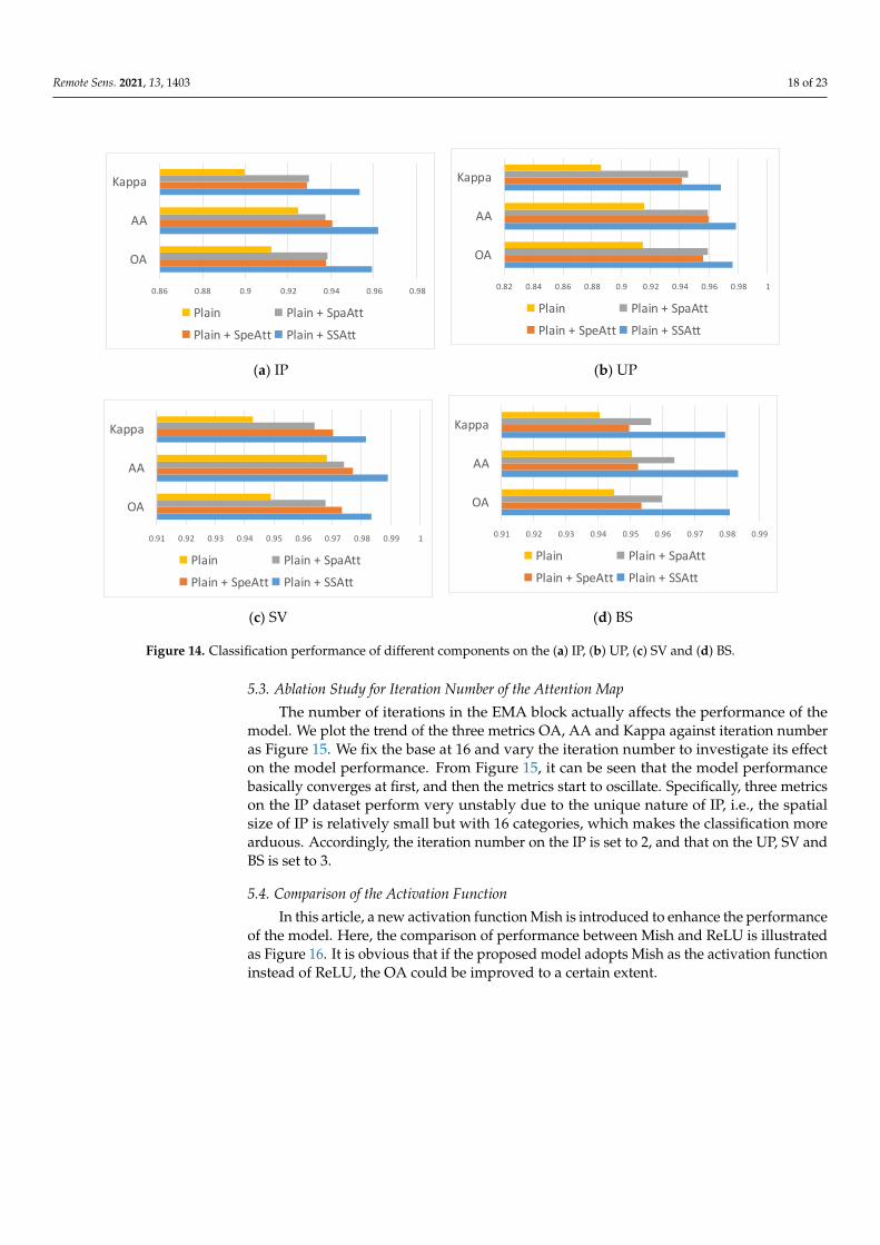
5.2. Investigation of the Attention Mechanism
Our model integrates spectral attention and spatial attention. In this section, we willtest the effectiveness of these attention modules. Specifically, we consider a PyConv-onlynetwork without any attention module as a baseline (denoted as Plain). It is a simpledouble-branch model that extracts spatial and spectral features separately. Moreover,we denote the three derivatives: the subnetwork integrated with spectral attention, thesubnetwork integrated with spatial attention and the subnetwork integrated with both asPlain + SpeAtt, Plain + SpaAtt and Plain + SSAtt, respectively.
Figure 14 shows the comparison of the classification results of different networks interms of OA, AA and Kappa. Different colors indicate different subnetworks. From thefigure, we can see that either spectral attention or spatial attention, once integrated intothe network, can contribute to the performance of the original network. This confirms theeffectiveness of the proposed attention module. In addition, we can observe that the Plain+ SSAt outperforms all the other subnetworks. This implies that spectral attention andspatial attention can complement each other to contribute more to the final classificationdecision.
Remote Sens. 2021, 13, 1403 18 of 23
Remote Sens. 2021, 13, x FOR PEER REVIEW 18 of 24
(c) SV (d) BS
Figure 13. The OA of SVM, CDCNN, FDSSC, DBDA and our method with different proportions of training samples on the (a) IP,
(b) UP, (c) SV and (d) BS.
5.2. Investigation of the Attention Mechanism
Our model integrates spectral attention and spatial attention. In this section, we will
test the effectiveness of these attention modules. Specifically, we consider a PyConv-only
network without any attention module as a baseline (denoted as Plain). It is a simple
double-branch model that extracts spatial and spectral features separately. Moreover, we
denote the three derivatives: the subnetwork integrated with spectral attention, the
subnetwork integrated with spatial attention and the subnetwork integrated with both as
Plain+SpeAtt, Plain+SpaAtt and Plain+SSAtt, respectively.
Figure 14 shows the comparison of the classification results of different networks in
terms of OA, AA and Kappa. Different colors indicate different subnetworks. From the
figure, we can see that either spectral attention or spatial attention, once integrated into
the network, can contribute to the performance of the original network. This confirms the
effectiveness of the proposed attention module. In addition, we can observe that the
Plain+SSAt outperforms all the other subnetworks. This implies that spectral attention
and spatial attention can complement each other to contribute more to the final
classification decision.
(a) IP (b) UP
75
80
85
90
95
100
0.50% 1% 3% 5% 10%
OA
(%)
Pecentage of training samples(%)
DBDA SVM CDCNN FDSSC Ours
70
75
80
85
90
95
100
0.50% 1% 3% 5% 10%
OA
(%)
Percentage of training samples(%)
DBDA SVM CDCNN FDSSC OURS
0.86 0.88 0.9 0.92 0.94 0.96 0.98
OA
AA
Kappa
Plain Plain + SpaAtt
Plain + SpeAtt Plain + SSAtt
0.82 0.84 0.86 0.88 0.9 0.92 0.94 0.96 0.98 1
OA
AA
Kappa
Plain Plain + SpaAtt
Plain + SpeAtt Plain + SSAttRemote Sens. 2021, 13, x FOR PEER REVIEW 19 of 24
(c) SV (d) BS
Figure 14. Classification performance of different components on the (a) IP, (b) UP, (c) SV and (d) BS.
5.3. Ablation Study for Iteration Number of the Attention Map
The number of iterations in the EMA block actually affects the performance of the
model. We plot the trend of the three metrics OA, AA and Kappa against iteration number
as Figure 15. We fix the base at 16 and vary the iteration number to investigate its effect
on the model performance. From Figure 15, it can be seen that the model performance
basically converges at first, and then the metrics start to oscillate. Specifically, three
metrics on the IP dataset perform very unstably due to the unique nature of IP, i.e., the
spatial size of IP is relatively small but with 16 categories, which makes the classification
more arduous. Accordingly, the iteration number on the IP is set to 2, and that on the UP,
SV and BS is set to 3.
(a) IP (b) UP
(c) SV (d) BS
Figure 15. OA, AA and Kappa of the proposed model with different iteration number on the (a) IP, (b) UP, (c) SV and (d)
BS.
0.91 0.92 0.93 0.94 0.95 0.96 0.97 0.98 0.99 1
OA
AA
Kappa
Plain Plain + SpaAtt
Plain + SpeAtt Plain + SSAtt
0.91 0.92 0.93 0.94 0.95 0.96 0.97 0.98 0.99
OA
AA
Kappa
Plain Plain + SpaAtt
Plain + SpeAtt Plain + SSAtt
0.7
0.75
0.8
0.85
0.9
0.95
1
1 2 3 4 5 6 7 8 9 10
Iteration number
OA AA KAPPA
0.7
0.75
0.8
0.85
0.9
0.95
1
1 2 3 4 5 6 7 8 9 10
Iteration number
OA AA KAPPA
0.7
0.75
0.8
0.85
0.9
0.95
1
1 2 3 4 5 6 7 8 9 10
Iteration number
OA AA KAPPA
0.7
0.75
0.8
0.85
0.9
0.95
1
1 2 3 4 5 6 7 8 9 10
Iteration number
OA AA KAPPA
Figure 14. Classification performance of different components on the (a) IP, (b) UP, (c) SV and (d) BS.
5.3. Ablation Study for Iteration Number of the Attention Map
The number of iterations in the EMA block actually affects the performance of themodel. We plot the trend of the three metrics OA, AA and Kappa against iteration numberas Figure 15. We fix the base at 16 and vary the iteration number to investigate its effecton the model performance. From Figure 15, it can be seen that the model performancebasically converges at first, and then the metrics start to oscillate. Specifically, three metricson the IP dataset perform very unstably due to the unique nature of IP, i.e., the spatialsize of IP is relatively small but with 16 categories, which makes the classification morearduous. Accordingly, the iteration number on the IP is set to 2, and that on the UP, SV andBS is set to 3.
5.4. Comparison of the Activation Function
In this article, a new activation function Mish is introduced to enhance the performanceof the model. Here, the comparison of performance between Mish and ReLU is illustratedas Figure 16. It is obvious that if the proposed model adopts Mish as the activation functioninstead of ReLU, the OA could be improved to a certain extent.

Remote Sens. 2021, 13, 1403 19 of 23
Remote Sens. 2021, 13, x FOR PEER REVIEW 19 of 24
(c) SV (d) BS
Figure 14. Classification performance of different components on the (a) IP, (b) UP, (c) SV and (d) BS.
5.3. Ablation Study for Iteration Number of the Attention Map
The number of iterations in the EMA block actually affects the performance of the
model. We plot the trend of the three metrics OA, AA and Kappa against iteration number
as Figure 15. We fix the base at 16 and vary the iteration number to investigate its effect
on the model performance. From Figure 15, it can be seen that the model performance
basically converges at first, and then the metrics start to oscillate. Specifically, three
metrics on the IP dataset perform very unstably due to the unique nature of IP, i.e., the
spatial size of IP is relatively small but with 16 categories, which makes the classification
more arduous. Accordingly, the iteration number on the IP is set to 2, and that on the UP,
SV and BS is set to 3.
(a) IP (b) UP
(c) SV (d) BS
Figure 15. OA, AA and Kappa of the proposed model with different iteration number on the (a) IP, (b) UP, (c) SV and (d)
BS.
0.91 0.92 0.93 0.94 0.95 0.96 0.97 0.98 0.99 1
OA
AA
Kappa
Plain Plain + SpaAtt
Plain + SpeAtt Plain + SSAtt
0.91 0.92 0.93 0.94 0.95 0.96 0.97 0.98 0.99
OA
AA
Kappa
Plain Plain + SpaAtt
Plain + SpeAtt Plain + SSAtt
0.7
0.75
0.8
0.85
0.9
0.95
1
1 2 3 4 5 6 7 8 9 10
Iteration number
OA AA KAPPA
0.7
0.75
0.8
0.85
0.9
0.95
1
1 2 3 4 5 6 7 8 9 10
Iteration number
OA AA KAPPA
0.7
0.75
0.8
0.85
0.9
0.95
1
1 2 3 4 5 6 7 8 9 10
Iteration number
OA AA KAPPA
0.7
0.75
0.8
0.85
0.9
0.95
1
1 2 3 4 5 6 7 8 9 10
Iteration number
OA AA KAPPA
Figure 15. OA, AA and Kappa of the proposed model with different iteration number on the (a) IP, (b) UP, (c) SV and (d) BS.
Remote Sens. 2021, 13, x FOR PEER REVIEW 20 of 24
(a) IP
(b) UP
(c) SV
(d) BS
Figure 15. OA, AA and Kappa of the proposed model with different iteration number on the (a) IP, (b) UP, (c) SV and (d) BS.
5.4. Comparison of the Activation Function
In this article, a new activation function Mish is introduced to enhance the
performance of the model. Here, the comparison of performance between Mish and ReLU
is illustrated as Figure 16. It is obvious that if the proposed model adopts Mish as the
activation function instead of ReLU, the OA could be improved to a certain extent.
Figure 16. Comparison of OA with activation functions Mish and ReLU on different datasets.
5.5. Comparison of Different Feature Fusion
As illustrated in Figure 17, concatenation outperforms overall. This is as expected, as
the spectral and spatial features are in the independent feature space. If addition operation
0.7
0.75
0.8
0.85
0.9
0.95
1
1 2 3 4 5 6 7 8 9 10
Iteration number
OA AA KAPPA
0.7
0.75
0.8
0.85
0.9
0.95
1
1 2 3 4 5 6 7 8 9 10
Iteration number
OA AA KAPPA
0.7
0.75
0.8
0.85
0.9
0.95
1
1 2 3 4 5 6 7 8 9 10
Iteration number
OA AA KAPPA
0.7
0.75
0.8
0.85
0.9
0.95
1
1 2 3 4 5 6 7 8 9 10
Iteration number
OA AA KAPPA
0.91 0.92 0.93 0.94 0.95 0.96 0.97 0.98 0.99
IP
UP
SV
BS
OA
Mish ReLU
Figure 16. Comparison of OA with activation functions Mish and ReLU on different datasets.
5.5. Comparison of Different Feature Fusion
As illustrated in Figure 17, concatenation outperforms overall. This is as expected,as the spectral and spatial features are in the independent feature space. If additionoperation is adopted instead of concatenation, information from different domains tendsto be intermixed or even interfere with each other. However, we can see that the additionoperation outperforms the concatenation operation on the IP dataset. At first it is attributedto a coincidence, nonetheless, the results remain the same after repeated experiments. Suchexperimental results may be caused by the specificity of the IP dataset, which has beenmentioned in Section 5.3. In contrast to the concatenation operation, weighted addition can

Remote Sens. 2021, 13, 1403 20 of 23
use weights to adjust the influence of spectral and spatial information on the classificationresults. This property is probably more useful for the IP dataset, since its spatial size issmallest while the numbers of spectral bands categories are large.
Remote Sens. 2021, 13, x FOR PEER REVIEW 21 of 24
is adopted instead of concatenation, information from different domains tends to be
intermixed or even interfere with each other. However, we can see that the addition
operation outperforms the concatenation operation on the IP dataset. At first it is
attributed to a coincidence, nonetheless, the results remain the same after repeated
experiments. Such experimental results may be caused by the specificity of the IP dataset,
which has been mentioned in Section 5.3. In contrast to the concatenation operation,
weighted addition can use weights to adjust the influence of spectral and spatial
information on the classification results. This property is probably more useful for the IP
dataset, since its spatial size is smallest while the numbers of spectral bands categories are
large.
Figure 17. Comparison of OA with different feature fusion operations.
5.6 Investigation of Running Time
A decent method should achieve a favorable accuracy-efficiency trade-off. In this
section, we will compare the time costs of the seven algorithms on the IP, UP, SV, and BS
datasets. Tables 5–8 show the training time and test time of seven methods on the four
datasets.
Table 5. The running time of seven methods on the IP dataset.
Dataset Algorithm Training Time (s) Testing Time (s)
IP
SVM 21.50 1.15
CDCNN 11.25 1.69
SSRN 82.98 3.45
FDSSC 122.94 4.51
DBMA 47.36 8.56
DBDA 64.64 7.98
Proposed 61.34 4.51
Table 6. The running time of seven methods on the UP dataset.
Dataset Algorithm Training Time (s) Testing Time (s)
UP
SVM 3.69 2.94
CDCNN 8.39 6.28
SSRN 20.45 10.18
FDSSC 53.84 12.78
DBMA 32.06 22.79
DBDA 16.03 21.09
Proposed 38.72 12.49
0.945 0.95 0.955 0.96 0.965 0.97 0.975 0.98 0.985 0.99
IP
UP
SV
BS
OA
Weighted addition Concatenation
Figure 17. Comparison of OA with different feature fusion operations.
5.6. Investigation of Running Time
A decent method should achieve a favorable accuracy-efficiency trade-off. In thissection, we will compare the time costs of the seven algorithms on the IP, UP, SV, and BSdatasets. Tables 5–8 show the training time and test time of seven methods on the fourdatasets.
Table 5. The running time of seven methods on the IP dataset.
Dataset Algorithm Training Time (s) Testing Time (s)
IP
SVM 21.50 1.15CDCNN 11.25 1.69
SSRN 82.98 3.45FDSSC 122.94 4.51DBMA 47.36 8.56DBDA 64.64 7.98
Proposed 61.34 4.51
Table 6. The running time of seven methods on the UP dataset.
Dataset Algorithm Training Time (s) Testing Time (s)
UP
SVM 3.69 2.94CDCNN 8.39 6.28
SSRN 20.45 10.18FDSSC 53.84 12.78DBMA 32.06 22.79DBDA 16.03 21.09
Proposed 38.72 12.49
From Tables 5–8, it can be observed that SVM spends less training time and test-ing time than DL-based methods in most cases. Furthermore, since 2D convolution ismore parameter- and computation-conserving than 3D convolution, CDCNN, as a rep-resentative of 2D-CNN-based methods, is more time-conserving than 3D-CNN-basedmethods. Among these five 3D-CNN-based methods, the training time and testing time ofour method are moderate. Considering the accuracy of our method is promising, it canbe concluded that the proposed method strikes a better balance between accuracy andefficiency.
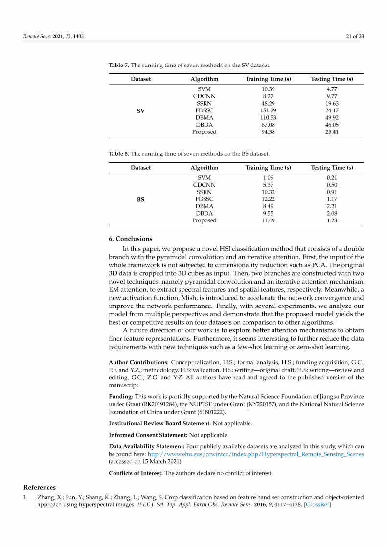
Remote Sens. 2021, 13, 1403 21 of 23
Table 7. The running time of seven methods on the SV dataset.
Dataset Algorithm Training Time (s) Testing Time (s)
SV
SVM 10.39 4.77CDCNN 8.27 9.77
SSRN 48.29 19.63FDSSC 151.29 24.17DBMA 110.53 49.92DBDA 67.08 46.05
Proposed 94.38 25.41
Table 8. The running time of seven methods on the BS dataset.
Dataset Algorithm Training Time (s) Testing Time (s)
BS
SVM 1.09 0.21CDCNN 5.37 0.50
SSRN 10.32 0.91FDSSC 12.22 1.17DBMA 8.49 2.21DBDA 9.55 2.08
Proposed 11.49 1.23
6. Conclusions
In this paper, we propose a novel HSI classification method that consists of a doublebranch with the pyramidal convolution and an iterative attention. First, the input of thewhole framework is not subjected to dimensionality reduction such as PCA. The original3D data is cropped into 3D cubes as input. Then, two branches are constructed with twonovel techniques, namely pyramidal convolution and an iterative attention mechanism,EM attention, to extract spectral features and spatial features, respectively. Meanwhile, anew activation function, Mish, is introduced to accelerate the network convergence andimprove the network performance. Finally, with several experiments, we analyze ourmodel from multiple perspectives and demonstrate that the proposed model yields thebest or competitive results on four datasets on comparison to other algorithms.
A future direction of our work is to explore better attention mechanisms to obtainfiner feature representations. Furthermore, it seems interesting to further reduce the datarequirements with new techniques such as a few-shot learning or zero-shot learning.
Author Contributions: Conceptualization, H.S.; formal analysis, H.S.; funding acquisition, G.C.,P.F. and Y.Z.; methodology, H.S; validation, H.S; writing—original draft, H.S; writing—review andediting, G.C., Z.G. and Y.Z. All authors have read and agreed to the published version of themanuscript.
Funding: This work is partially supported by the Natural Science Foundation of Jiangsu Provinceunder Grant (BK20191284), the NUPTSF under Grant (NY220157), and the National Natural ScienceFoundation of China under Grant (61801222).
Institutional Review Board Statement: Not applicable.
Informed Consent Statement: Not applicable.
Data Availability Statement: Four publicly available datasets are analyzed in this study, which canbe found here: http://www.ehu.eus/ccwintco/index.php/Hyperspectral_Remote_Sensing_Scenes(accessed on 15 March 2021).
Conflicts of Interest: The authors declare no conflict of interest.
References1. Zhang, X.; Sun, Y.; Shang, K.; Zhang, L.; Wang, S. Crop classification based on feature band set construction and object-oriented
approach using hyperspectral images. IEEE J. Sel. Top. Appl. Earth Obs. Remote Sens. 2016, 9, 4117–4128. [CrossRef]

Remote Sens. 2021, 13, 1403 22 of 23
2. Stuart, M.B.; McGonigle, A.J.S.; Willmott, J.R. Hyperspectral imaging in environmental monitoring: A review of recent develop-ments and technological advances in compact field deployable systems. Sensors 2019, 19, 3071. [CrossRef] [PubMed]
3. Carter, G.A.; Lucas, K.L.; Blossom, G.A.; Holiday, C.L.L.; Mooneyhan, D.S.; Fastring, D.R.; Holcombe, T.R.; Griffith, J.A. Remotesensing and mapping of tamarisk along the colorado river, USA: A comparative use of summer-acquired hyperion, thematicmapper and quickbird data. Remote Sens. 2009, 1, 318–329. [CrossRef]
4. Tu, B.; Wang, J.; Kang, X.; Zhang, G.; Ou, X.; Guo, L. KNN-based representation of superpixels for hyperspectral imageclassification. IEEE J. Sel. Top. Appl. Earth Obs. Remote Sens. 2018, 11, 4032–4047. [CrossRef]
5. Li, J.; Bioucas-Dias, J.M.; Plaza, A. Spectral-spatial hyperspectral image segmentation using subspace multinomial logisticregression and markov random fields. IEEE Trans. Geosci. Remote Sens. 2012, 50, 809–823. [CrossRef]
6. Melgani, F.; Bruzzone, L. Classification of hyperspectral remote sensing images with support vector machines. IEEE Trans. Geosci.Remote Sens. 2004, 42, 1778–1790. [CrossRef]
7. Fauvel, M.; Zullo, A.; Ferraty, F. Nonlinear parsimonious feature selection for the classification of hyperspectral images. InProceedings of the 6th Workshop on Hyperspectral Image and Signal Processing: Evolution in Remote Sensing (WHISPERS),Lausanne, Switzerland, 24–27 June 2014; pp. 1–4. [CrossRef]
8. Khan, Z.; Shafait, F.; Mian, A. Joint group sparse PCA for compressed hyperspectral imaging. IEEE Trans. Image Process. 2015, 24,4934–4942. [CrossRef]
9. Gu, Y.; Wang, C.; You, D.; Zhang, Y.; Wang, S.; Zhang, Y. Representative multiple kernel learning for classification in hyperspectralimagery. IEEE Trans. Geosci. Remote Sens. 2012, 50, 2852–2865. [CrossRef]
10. Fang, L.; Li, S.; Duan, W.; Ren, J.; Benediktsson, J.A. Classification of hyperspectral images by exploiting spectral-spatialinformation of superpixel via multiple kernels. IEEE Trans. Geosci. Remote Sens. 2015, 53, 6663–6674. [CrossRef]
11. Yu, H.; Gao, L.; Liao, W.; Zhang, B.; Pizurica, A.; Philips, W. Multiscale superpixel-level subspace-based support vector machinesfor hyperspectral image classification. IEEE Geosci. Remote Sens. Lett. 2017, 14, 2142–2146. [CrossRef]
12. Zhang, L.; Zhang, L.; Du, B. Deep learning for remote sensing data: A technical tutorial on the state of the art. IEEE Geosci. RemoteSens. Mag. 2016, 4, 22–40. [CrossRef]
13. Tan, M.; Pang, R.; Le, Q.V. EfficientDet: Scalable and efficient object detection. In Proceedings of the IEEE Computer SocietyConference on Computer Vision and Pattern Recognition, San Juan, PR, USA, 14–19 June 2020. [CrossRef]
14. Zhao, H.; Shi, J.; Qi, X.; Wang, X.; Jia, J. Pyramid scene parsing network. In Proceedings of the 30th IEEE Conference on ComputerVision and Pattern Recognition, CVPR 2017, Honolulu, HI, USA, 21–26 July 2017. [CrossRef]
15. Karras, T.; Laine, S.; Aila, T. A Style-Based Generator Architecture for Generative Adversarial Networks. In Proceedings ofthe IEEE Computer Society Conference on Computer Vision and Pattern Recognition, Long Beach, CA, USA, 16–20 June 2019.[CrossRef]
16. Chen, Y.; Lin, Z.; Zhao, X.; Wang, G.; Gu, Y. Deep learning-based classification of hyperspectral data. IEEE J. Sel. Top. Appl. EarthObs. Remote Sens. 2014, 7, 2094–2107. [CrossRef]
17. Zhao, C.; Wan, X.; Zhao, G.; Cui, B.; Liu, W.; Qi, B. Spectral-spatial classification of hyperspectral imagery based on stacked sparseautoencoder and random forest. Eur. J. Remote Sens. 2017, 50, 47–63. [CrossRef]
18. Li, T.; Zhang, J.; Zhang, Y. Classification of hyperspectral image based on deep belief networks. In Proceedings of the 2014 IEEEInternational Conference on Image Processing, ICIP 2014, Paris, France, 27–30 October 2014; pp. 5132–5136. [CrossRef]
19. Zhong, P.; Gong, Z.; Li, S.; Schonlieb, C.B. Learning to diversify deep belief networks for hyperspectral image classification. IEEETrans. Geosci. Remote Sens. 2017, 55, 3516–3530. [CrossRef]
20. Yu, C.; Zhao, M.; Song, M.; Wang, Y.; Li, F.; Han, R.; Chang, C.I. Hyperspectral image classification method based on cnnarchitecture embedding with hashing semantic feature. IEEE J. Sel. Top. Appl. Earth Obs. Remote Sens. 2019, 12, 1866–1881.[CrossRef]
21. Mei, S.; Ji, J.; Bi, Q.; Hou, J.; Du, Q.; Li, W. Integrating spectral and spatial information into deep convolutional neural networksfor hyperspectral classification. In Proceedings of the International Geoscience and Remote Sensing Symposium (IGARSS),Beijing, China, 10–15 July 2016; pp. 5067–5070. [CrossRef]
22. Lee, H.; Kwon, H. Going deeper with contextual CNN for hyperspectral image classification. IEEE Trans. Image Process. 2017, 26,4843–4855. [CrossRef]
23. Zhao, W.; Du, S. Spectral-spatial feature extraction for hyperspectral image classification: A dimension reduction and deeplearning approach. IEEE Trans. Geosci. Remote Sens. 2016, 54, 4544–4554. [CrossRef]
24. Ben Hamida, A.; Benoit, A.; Lambert, P.; Ben Amar, C. 3-D deep learning approach for remote sensing image classification. IEEETrans. Geosci. Remote Sens. 2018, 56, 4420–4434. [CrossRef]
25. Zhong, S.; Chen, S.; Chang, C.-I.; Zhang, Y. Fusion of spectral-spatial classifiers for hyperspectral image classification. IEEE Trans.Geosci. Remote Sens. 2020, 1–20. [CrossRef]
26. He, K.; Zhang, X.; Ren, S.; Sun, J. Deep residual learning for image recognition. In Proceedings of the IEEE Conference onComputer Vision and Pattern Recognition, Las Vegas, NV, USA, 26 June–1 July 2016; pp. 770–778. [CrossRef]
27. Huang, G.; Liu, Z.; Van Der Maaten, L.; Weinberger, K.Q. Densely connected convolutional networks. In Proceedings of the IEEEConference on Computer Vision and Pattern Recognition, Honolulu, HI, USA, 21–26 July 2017; pp. 4700–4708. [CrossRef]
28. Zhong, Z.; Li, J.; Luo, Z.; Chapman, M. Spectral-spatial residual network for hyperspectral image classification: A 3-D deeplearning framework. IEEE Trans. Geosci. Remote Sens. 2018, 56, 847–858. [CrossRef]
Remote Sens. 2021, 13, 1403 23 of 23
29. Fang, B.; Li, Y.; Zhang, H.; Chan, J.C.W. hyperspectral images classification based on dense convolutional networks withspectral-wise attention mechanism. Remote Sens. 2019, 11, 159. [CrossRef]
30. Zheng, Y.; Li, J.; Li, Y.; Guo, J.; Wu, X.; Chanussot, J. Hyperspectral pansharpening using deep prior and dual attention residualnetwork. IEEE Trans. Geosci. Remote Sens. 2020, 58, 8059–8076. [CrossRef]
31. Haut, J.M.; Paoletti, M.E.; Plaza, J.; Plaza, A.; Li, J. Visual attention-driven hyperspectral image classification. IEEE Trans. Geosci.Remote Sens. 2019, 57, 8065–8080. [CrossRef]
32. Sun, H.; Zheng, X.; Lu, X.; Wu, S. Spectral-spatial attention network for hyperspectral image classification. IEEE Trans. Geosci.Remote Sens. 2020, 58, 3232–3245. [CrossRef]
33. Ma, W.; Yang, Q.; Wu, Y.; Zhao, W.; Zhang, X. Double-branch multi-attention mechanism network for hyperspectral imageclassification. Remote Sens. 2019, 11, 1307. [CrossRef]
34. Fu, J.; Liu, J.; Tian, H.; Li, Y.; Bao, Y.; Fang, Z.; Lu, H. Dual attention network for scene segmentation. In Proceedings of theIEEE Computer Society Conference on Computer Vision and Pattern Recognition, Long Beach, CA, USA, 16–20 June 2019;pp. 3141–3149. [CrossRef]
35. Li, R.; Zheng, S.; Duan, C.; Yang, Y.; Wang, X. Classification of hyperspectral image based on double-branch dual-attentionmechanism network. Remote Sens. 2020, 12, 582. [CrossRef]
36. Tran, D.; Bourdev, L.; Fergus, R.; Torresani, L.; Paluri, M. Learning spatiotemporal features with 3d convolutional networks.In Proceedings of the IEEE International Conference on Computer Vision, ICCV 2015, Santiago, Chile, 7–13 December 2015;pp. 4489–4497. [CrossRef]
37. Ying, X.; Wang, L.; Wang, Y.; Sheng, W.; An, W.; Guo, Y. Deformable 3D convolution for video super-resolution. IEEE Signal.Process. Lett. 2020, 27, 1500–1504. [CrossRef]
38. Molchanov, P.; Yang, X.; Gupta, S.; Kim, K.; Tyree, S.; Kautz, J. Online detection and classification of dynamic hand gestures withrecurrent 3D convolutional neural networks. In Proceedings of the IEEE Computer Society Conference on Computer Vision andPattern Recognition, CVPR 2016, Las Vegas, NV, USA, 27–30 June 2016. [CrossRef]
39. Ge, C.; Qu, Q.; Gu, I.Y.H.; Store Jakola, A. 3D multi-scale convolutional networks for glioma grading using MR images. InProceedings of the International Conference on Image Processing(ICIP), Athens, Greece, 7–10 October 2018. [CrossRef]
40. Duta, I.C.; Liu, L.; Zhu, F.; Shao, L. Pyramidal convolution: Rethinking convolutional neural networks for visual recognition.arXiv 2020, arXiv:2006.11538, 1–16.
41. Wang, X.; Girshick, R.; Gupta, A.; He, K. Non-local neural networks. In Proceedings of the IEEE Conference on Computer Visionand Pattern Recognition, CVPR 2017, Honolulu, HI, USA, 21–26 July 2017; pp. 7794–7803. [CrossRef]
42. Vaswani, A.; Shazeer, N.; Parmar, N.; Uszkoreit, J.; Jones, L.; Gomez, A.N.; Kaiser, Ł.; Polosukhin, I. Attention is all you need.arXiv 2017, arXiv:1706.03762, 5999–6009.
43. Zhao, H.; Zhang, Y.; Liu, S.; Shi, J.; Loy, C.C.; Lin, D.; Jia, J.; Zhao, H.; Zhang, Y.; Liu, S.; et al. PSANet: Point-wise spatial attentionnetwork for scene parsing—Supplementary material. In Proceedings of the European Conference on Computer Vision (ECCV),Munich, Germany, 8–14 September 2018; pp. 267–283.
44. Chen, Y.; Kalantidis, Y.; Li, J.; Yan, S.; Feng, J. A2-Nets: Double attention networks. arXiv 2018, arXiv:1810.11579, 352.45. Li, X.; Zhong, Z.; Wu, J.; Yang, Y.; Lin, Z.; Liu, H. Expectation-maximization attention networks for semantic segmentation. In
Proceedings of the IEEE/CVF International Conference on Computer Vision, ICCV 2019, Seoul, Korea, 27 October–2 November2019; pp. 9166–9175. [CrossRef]
46. Misra, D. Mish: A self regularized non-monotonic neural activation function. arXiv 2019, arXiv:1908.08681.47. He, K.; Zhang, X.; Ren, S.; Sun, J. Delving deep into rectifiers: Surpassing human-level performance on imagenet classification. In
Proceedings of the IEEE Conference on Computer Vision and Pattern Recognition, CVPR 2015, Boston, MA, USA, 7–12 June 2015.[CrossRef]
48. Srivastava, N.; Hinton, G.; Krizhevsky, A.; Sutskever, I.; Salakhutdinov, R. Dropout: A simple way to prevent neural networksfrom overfitting. J. Mach. Learn. Res. 2014, 15, 1929–1958.
49. Loshchilov, I.; Hutter, F. SGDR: Stochastic gradient descent with warm restarts. In Proceedings of the 5th International Conferenceon Learning Representations, ICLR 2017—Conference Track Proceedings, Toulon, France, 24–26 April 2017.