INVESTIGATING THE PRODUCTIVITY MIRACLE USING

MULTINATIONALS

Nick Bloom1, Raffaella Sadun2 and John Van Reenen2 1 Stanford, Centre for Economic Performance and NBER 2 London School of Economics and Centre for Economic Performance

August 2006

Abstract

Productivity growth in sectors that intensively use information technologies (IT) appears to have accelerated much faster in the US than in Europe since 1995, leading to the US “productivity miracle”. If this was partly due to the superior management or organization of US firms (rather than simply the advantages of being located in the US geographically) we would expect to see a stronger association of productivity with IT for US multinationals (compared to non-US multinationals) located in Europe. We examine a large panel of UK establishments and provide evidence that US owned establishments do indeed have a stronger relationship between productivity and IT capital than either non-US multinationals or domestic establishments. Indeed, the differential effect of IT appears to account for almost all the difference in total factor productivity between US-owned and all other establishments. This finding holds in the cross section, when including fixed effects and even when we examine a sample of establishments taken over by US multinationals. We find that the US multinational effect on IT is particularly strong in the sectors that intensively use information technologies (such as retail and wholesale): the very same industries that accounted for the US-European productivity growth differential since the mid 1990s. Key words: Productivity, IT, multinationals, organization. JEL classification: E22, O3, O47, O52 Acknowledgments We would like to thank Tony Clayton for support and helpful discussions and Mary O’ Mahony for providing the NIESR Industry data. We would like to thank the Department of Trade and Industry and the Economic and Social Research Council for financial support. Helpful comments have been given by Tim Bresnahan, Eric Brynjolfsson, John Haltiwanger, Rupert Harrison, Jonathan Haskel, Dale Jorgensen, Rob Moffitt, Nick Oulton, Mark Schankerman, Paul Seabright, Johannes von Biesebroeck, Manuel Trajtenberg and participants at a range of seminars. This work contains statistical data from the Office of National Statistics (ONS) which is Crown copyright and reproduced with the permission of the controller of HMSO and Queens Printer for Scotland. The use of the ONS statistical data in this work does not imply the endorsement of the ONS in relation to the interpretation or analysis of the statistical data.

2

I. INTRODUCTION

“The 1995-2001 acceleration [in US productivity] may be plausibly accounted for by a

pickup in capital services per hour worked and by increases in organizational capital, the

investments businesses make to reorganize and restructure themselves, in this instance in

response to newly installed information technology”

Economic Report of the President, February 2006, p.26

One of the most startling economic facts of the last decade has been the reversal in the long-

standing catch-up of European countries’ productivity with the US. After slowing down after 174,

American Labour productivity growth accelerated after 1995 whereas Europe’s did not (see Figure

1). Decompositions of US productivity growth show that the great majority has occurred in those

sectors that either intensively use or produce IT (information technologies)1. Figure 2 shows that

US IT intensity appears to be consistently higher in the US than Europe and this gap has widened

over time. Closer analysis has shown that European countries had a similar productivity

acceleration as the US in IT producing sectors but failed to achieve the spectacular levels of

productivity growth in the sectors that used IT intensively (predominantly market service sectors

include retail, wholesale and financial intermediation). We show this in Figure 3. Given the

common availability of IT throughout the world at broadly similar prices, it is a major puzzle to

explain why these IT related productivity effects have not been more widespread.

Assuming that the difference in Europe’s relative productivity performance is not simply mis-

measurement2, then at least two explanations are possible. First, there are some “natural

advantages” to the environment in which US plants operate that enables them to take better

advantage of the opportunity of rapidly falling IT prices. These natural advantages could be tougher

product market competition, lower regulation in the product and labour markets, better access to

1 See, for example, Stiroh (2002). Jorgenson (2001), Oliner and Sichel (2001). In the 2002-2004 period Oliner and Sichel (2004) find that the US productivity growth remained strong, but there was a more widespread increase in productivity growth across sectors. See Gordon (2004) for a general discussion. 2 One explanation is simply differences in the way we measure productivity across countries (Blanchard, 2004). This is possible, but the careful work of O’Mahony and Van Ark (2003) and others who focus on the same sectors in the US and EU, use US-style adjustments for hedonic prices, software capitalization and aggregate demand conditions, still find a difference.

3

risk capital, more educated workers, larger market size, more geographical space or a host of other

factors. A second class of explanations stresses that it is not the US environment per se that matters

but rather the internal organization (the depth of “organizational capital”) of US firms that has

enabled better exploitation of IT. For example, US firms may be simply better managed or they

have adopted features that are better at exploiting IT (e.g. more decentralization or flatter

hierarchies)3.

Although these explanations are not mutually exclusive, one way to test whether “US firm

organization” hypotheses has any validity is to examine the IT performance of American owned

organizations in a non-US environment. Assuming that US multinationals at least partially export

their business models outside the US – and a walk into McDonalds or Starbucks anywhere in

Europe suggests that this is not an entirely unreasonable assumption – then analyzing the IT

performance of US multinational establishments in Europe should be informative. If we still

observe a systematically better use of IT in a non-US environment then this is consistent with the

“US firm organization” model. We return to the origins of differences in European vs. US

organizational forms in the conclusion.

In this paper we examine the productivity of IT in a panel of establishments located in the UK,

examining the differences in IT intensity and productivity between plants owned by US

multinationals, plants owned by non-US multinationals and domestic plants. The UK poses a useful

testing ground because (a) it has not experienced a US-style productivity acceleration since 1995 (as

Basu et al (2003) show); (b) it is a large recipient of foreign direct investment so we are able to

compare across many types of ownership; and (c) it has high levels of mergers and acquisition

activity producing frequent establishment ownership change. A key comparison group for US

multinationals are “statistically similar” non-US multinationals (i.e. establishments in the same

industry, of a similar age, size and factor intensity). We report evidence that the key difference in

understanding productivity differences is the ability of US multinationals to gain a higher

productivity impact from IT than non-US multinationals (and domestic plants). This effect is

strongest in precisely those industries that experienced the largest relative productivity gains in the

3 Bresnahan, Brynjolfsson and Hitt (2002) and Caroli and Van Reenen (2001) both find that internal organization and other complementary factors such as skills are important in generating significant returns to ICT.

4

US after 1995 (the sectors that intensively used IT). This finding is robust to a number of tests

including examining British plants before and after they have been taken over by a US

multinational compared to US takeovers (compared to being taken by a non-US multinational or

other kind of firm). In short, we conclude that the higher productivity of IT in the US is not just the

US environment, but also has something to do with the internal organization of US firms.

Some preliminary evidence on the importance of different internal organization of US firms can be

seen in Figures 4 and 5. This uses data on the internal organizational of over 700 firms in the US

and Europe. Figure 4a shows that, on average, firms operating in the US are more decentralized

than those operating in Europe4. In Figure 4b, we break down the latter into purely Domestic

European firms, subsidiaries of European multinationals and subsidiaries of US multinationals.

Interestingly, the degree of decentralization of US multinational subsidiaries in Europe is similar to

US firms as a whole and is significantly higher than the degree of decentralization of European

multinationals (and domestic European firms). In Figure 5 we use a composite measure of

management best practices (see Bloom and Van Reenen, 2006, for details). A similar picture

emerges – management quality is higher in the US and higher for US multinational subsidiaries in

Europe than European subsidiaries.

Although our focus is in accounting for the difference in macro productivity trends using micro

data, our paper related to three other literatures. First, there is a large literature on the impact of IT

on productivity, but most of this is based on data aggregated to the industry or macro-economic

level. Even the pioneering work of Brynjolfsson5 and his co-authors focuses at the firm level which

may conceal much heterogeneity between plants within firms. In this paper we provide, for the first

time, estimates for the level and the productivity impact of IT capital stocks for a panel of around

11,000 establishments, probably the largest micro-based sample in the world for this kind of

exercise. Our database, unlike the US LRD, also covers the non-manufacturing sector, which is

important as the majority of sectors that use IT intensively are in services.

4 Decentralization was measured in the same way as Bresnahan et al (2002) using questions related to task allocation and pace setting in order to indicate the degree of employee autonomy. See notes to the Figures for details. 5 Brynjolfsson and Hitt (1995, 2003), Brynjolfsson, Hitt and Yang (2002). Brynjolfsson and Yang (1996) or Stiroh (2004) survey the evidence.

5

Second, in a reversal of the Solow Paradox, the firm level productivity literature has found returns

to IT that are larger than one would expect under the standard growth accounting assumptions.

Brynjolfsson and Hitt (2003) argue that this is due to complementary investments in “organizational

capital” that are reflected in the coefficients on IT capital. Almost all of these studies are on US

firms, however, and the data used is generally prior to the post 1995 acceleration in productivity

growth. Examining UK firms that may have made fewer complementary investments we might

expect to see lower returns (Basu et al, 2003).

Thirdly, there is a literature on the productivity of multinationals compared to similar non-

multinational establishments. The first wave of research that compared domestic plants with

multinationals was clearly misleading as multinationals are a self-selected group that have some

additional efficiency as signaled by their ability to operate overseas. But comparing across different

multinationals it appears that US plants are more productive whether based geographically in the

US (Doms and Jensen, 1998) or in other parts of the world such as the UK (e.g. Criscuolo and

Martin, 2005). Our paper suggests that the major reason for this American multinational

productivity advantage is the way in which US multinationals are able to use new technologies

more effectively than other multinationals.

In summary, we do find significant impacts of IT on productivity. We also find that we can account

for almost all of the higher productivity of US multinationals by the higher productivity impact of

their use of IT. Furthermore, this US advantage is strongest in the sectors that intensively use IT:

precisely those sectors that account for the faster productivity growth in the US than Europe since

1995. This suggests that at least some of the differential performance of productivity between the

US and the EU since the mid 1990s is due to the internal organization of US firms. Drawing on

some of our other work we show that there is evidence for significant differences in the

“organizational capital” of US firms relative to British and other European firms, even when these

US firms operate in Europe.

The structure of this paper is as follows. Section II discusses the empirical framework, section III

the data and section IV gives the main results. In section V we sketch a simple model that can

account for the stylized facts we see in the data. Finally, section VI offers some conclusions.

6

II. EMPRICIAL MODELLING STRATEGY

II.A. Basic Approach

We assume that the basic production function can be written as follows

itCitit

Kitit

Litit

Mititit cklmaq ~~~~~~ αααα ++++= (1)

where titit XXx lnln~ −≡ is the logarithmic deviations from the year-specific industry mean (which

control for input and output prices).6 Q is gross output, A is an establishment specific productivity

factor, M is materials, L is labor, K is non-IT fixed capital and C is computer/IT capital.

We are particularly interested in the role of IT capital and whether the impact of computers on

productivity is systematically higher for the plants belonging to US firms in the sectors that

intensively use IT and that appear to have been responsible for the bulk of the US productivity

acceleration since the mid 1990s. Consider parameterizing the output elasticities in equation (1) as:

MNEit

MNEJh

USAit

USAJh

Jh

Jit DD ,,0, αααα ++= (2)

where USAitD denotes that the establishment is owned by a US firm in year t and MNE

itD denotes that

the establishment is owned by a non-US multinational enterprise (the base case is that firm is a non-

multinational purely domestic firm), the sub-script h denotes sector (e.g. industries that use IT

intensively vs. non-IT intensive sectors) and the super-script J indicates a particular factor of

production (M, L, K, C). We further assume that total plant specific efficiency can be written as:

ithithMNEit

MNEh

USAit

USAhhiit uzDDaa ,

0 ~'~ +++++= γδδδ (3)

6 See Klette (1999) for a detailed discussion of this approach.

7

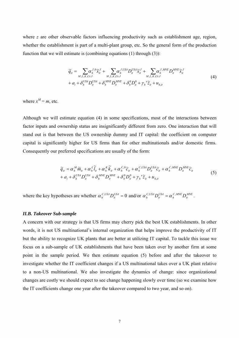
where z are other observable factors influencing productivity such as establishment age, region,

whether the establishment is part of a multi-plant group, etc. So the general form of the production

function that we will estimate is (combining equations (1) through (3)):

ithithithMNEit

MNEh

USAit

USAhi

JCKLM

Jit

MNEit

MNEJh

JCKLM

Jit

USAit

USAJh

JCKLM

Jit

Jhit

uzDDDa

xDxDxq

,00

,,,

,

,,,

,

,,,

0,

~'

~~~~

++++++

++= ∑∑∑∈∈∈

γδδδ

ααα (4)

where xM = m, etc.

Although we will estimate equation (4) in some specifications, most of the interactions between

factor inputs and ownership status are insignificantly different from zero. One interaction that will

stand out is that between the US ownership dummy and IT capital: the coefficient on computer

capital is significantly higher for US firms than for other multinationals and/or domestic firms.

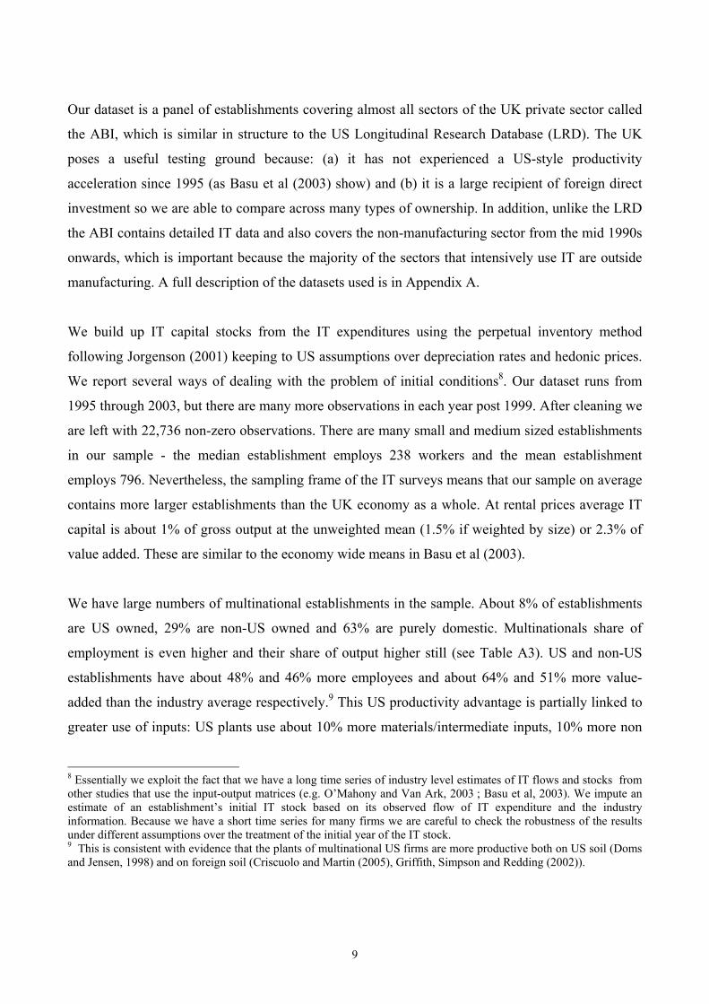
Consequently our preferred specifications are usually of the form:

ithithithMNEit

MNEh

USAit

USAhi

itMNEit

MNEChit

USAit

USAChit

Chit

Khit

Lhit

Mhit

uzDDDa

cDcDcklmq

,00

,,0,

~'

~~~~~~~

++++++

+++++=

γδδδ

αααααα (5)

where the key hypotheses are whether 0, =USAit

USACh Dα and/or MNE

itMNEC

hUSAit

USACh DD ,, αα = .

II.B. Takeover Sub-sample

A concern with our strategy is that US firms may cherry pick the best UK establishments. In other

words, it is not US multinational’s internal organization that helps improve the productivity of IT

but the ability to recognize UK plants that are better at utilizing IT capital. To tackle this issue we

focus on a sub-sample of UK establishments that have been taken over by another firm at some

point in the sample period. We then estimate equation (5) before and after the takeover to

investigate whether the IT coefficient changes if a US multinational takes over a UK plant relative

to a non-US multinational. We also investigate the dynamics of change: since organizational

changes are costly we should expect to see change happening slowly over time (so we examine how

the IT coefficients change one year after the takeover compared to two year, and so on).

8

The identification assumption here is not that establishments who are taken are the same as

establishments who are not taken over (the taken over tend to be less productive). Rather, we are

assuming that US multinationals are not systematically better than non-US multinationals at

successfully predicting (pre-takeover) the higher productivity of IT two or three years hence for

statistically identical British establishments. We regard this as a plausible assumption, but if US

managers did possess such foresight (and we will show that it is only for IT that the US takeovers

appear to be different than non-Us multinationals), it is not identified from the more general

organizational superiority of American firms.

II.C. Unobserved Heterogeneity

In all specifications we allow for a general structure of the error term that allows for arbitrary

heteroscedacity and autocorrelation over time. But there could still be establishment specific

unobserved heterogeneity. So we also generally include a full set of establishment level fixed

effects (the “within groups” estimator). The fixed effects estimators are more rigorous as there may

be many unobservable omitted variables correlated with IT that generate an upwards bias to the

coefficient on computer capital. On the other hand, attenuation bias (caused by measurement error

in IT and other right hand side variables) will be exacerbated by including fixed effects generating a

bias towards zero7.

II.D. Endogeneity of the Factor Inputs

We also want to allow for endogeneity of the factor inputs and take several approaches to dealing

with this issue. Our preferred measure is to use the “System GMM” estimator of Blundell and Bond

(1998) but we also compare this to a version of the Olley Pakes (1996) estimator. These methods

are detailed in Appendix A.

III. DATA

7 See Griliches and Mairesse (1998) for a general discussion of this problem with production functions and Brynjolfsson and Hitt, 1995, 1996, 2003) for a discussion specifically on IT.

9

Our dataset is a panel of establishments covering almost all sectors of the UK private sector called

the ABI, which is similar in structure to the US Longitudinal Research Database (LRD). The UK

poses a useful testing ground because: (a) it has not experienced a US-style productivity

acceleration since 1995 (as Basu et al (2003) show) and (b) it is a large recipient of foreign direct

investment so we are able to compare across many types of ownership. In addition, unlike the LRD

the ABI contains detailed IT data and also covers the non-manufacturing sector from the mid 1990s

onwards, which is important because the majority of the sectors that intensively use IT are outside

manufacturing. A full description of the datasets used is in Appendix A.

We build up IT capital stocks from the IT expenditures using the perpetual inventory method

following Jorgenson (2001) keeping to US assumptions over depreciation rates and hedonic prices.

We report several ways of dealing with the problem of initial conditions8. Our dataset runs from

1995 through 2003, but there are many more observations in each year post 1999. After cleaning we

are left with 22,736 non-zero observations. There are many small and medium sized establishments

in our sample - the median establishment employs 238 workers and the mean establishment

employs 796. Nevertheless, the sampling frame of the IT surveys means that our sample on average

contains more larger establishments than the UK economy as a whole. At rental prices average IT

capital is about 1% of gross output at the unweighted mean (1.5% if weighted by size) or 2.3% of

value added. These are similar to the economy wide means in Basu et al (2003).

We have large numbers of multinational establishments in the sample. About 8% of establishments

are US owned, 29% are non-US owned and 63% are purely domestic. Multinationals share of

employment is even higher and their share of output higher still (see Table A3). US and non-US

establishments have about 48% and 46% more employees and about 64% and 51% more value-

added than the industry average respectively.9 This US productivity advantage is partially linked to

greater use of inputs: US plants use about 10% more materials/intermediate inputs, 10% more non

8 Essentially we exploit the fact that we have a long time series of industry level estimates of IT flows and stocks from other studies that use the input-output matrices (e.g. O’Mahony and Van Ark, 2003 ; Basu et al, 2003). We impute an estimate of an establishment’s initial IT stock based on its observed flow of IT expenditure and the industry information. Because we have a short time series for many firms we are careful to check the robustness of the results under different assumptions over the treatment of the initial year of the IT stock. 9 This is consistent with evidence that the plants of multinational US firms are more productive both on US soil (Doms and Jensen, 1998) and on foreign soil (Criscuolo and Martin (2005), Griffith, Simpson and Redding (2002)).

10

IT capital and 27% more IT capital than non-US multinationals. Hence, US multinationals are

notably more IT intensive than other multinational subsidiaries.

We started by running a wide range of investigative OLS, GMM system and Olley-Pakes

production function estimations, displayed in full in Appendix A4. In summary, the different

estimators produced estimates of the elasticity of output with respect to IT in the range of 0.02 to

0.04. It is reassuring that productivity does indeed have a positive and significant association with

IT capital, consistent with the findings from several micro studies in the US and elsewhere.

Although the coefficient is larger than the share of IT capital in output (which is about 1% for our

firms) the difference is not as dramatic as has been found in other studies such as Brynjolfsson and

Hitt (2003)10. We will discuss possible reasons for this below, but an obvious reason is that IT

impacts may be heterogeneous between US firms and non-US firms.

We also considered several experiments changing our assumptions concerning the construction of

the IT capital stock. First, there is uncertainty over the exact depreciation rate for IT capital, so we

experimented with a number of alternatives including the extreme case of 100% depreciation and

just working with the flows. Second, we do not know the initial IT capital stock for ongoing firms

the first time they enter the sample. Our base method is to impute the initial year’s IT stock using as

a weight the firm’s observed IT investment relative to the industry IT investment. An alternative is

to assume that the plant’s share of the industry IT stock is the same as its share of employment in

the industry. In both cases this affected the magnitude of the coefficient on IT, but it always

remained positive and significant. In the results section below we analyze a third method where we

use an entirely different measure of IT use based on the number of workers in the establishment

using computers (from a different survey). This also gives similar results.

10 There are a number of possible reasons for the differences. Most obviously, Brynjolfsson’s data is from the US whereas ours is from the UK- we show that there appears to be larger IT coefficients for US firms than for UK firms. Other differences include (a) we are using more disaggregated data (establishments rather than worldwide accounts of firms); (b) our measure of IT capital is constructed in the standard way from flows of expenditure whereas Brynjolfsson and Hitt use a measure based on pricing different pieces of IT equipment; (c) our sample is much larger and covers a more recent time period and (d) our estimation techniques are different. We investigate some of these below.

11

IV. RESULTS IV.A. US Multinationals, IT and productivity

Table 1 contains the key results for the paper which is the productivity advantage of US

multinationals is linked to the use of IT. Column (1) estimates the basic production function

including a dummy variables for whether or not the plant was owned by a US multinational

(“USA”) or a non-US multinational (“MNE”) with plants who are domestic being the omitted base.

US establishments are 8.5% more productive than UK domestic establishments and non-US

multinationals are 4.8% more productive. The difference between the US and non US MNE

coefficients is also significant at the 1% level (p-value =0.001).

The second column of Table 1 includes the IT hardware measure which enters significantly and

reduces the coefficients on the ownership dummies. US plants are more IT intensive than other

plants and this explains some of the productivity gap. But it only accounts for about 12% of the

initial gap, i.e. about one percentage point of initial 8.5% productivity gap. Column (3) includes two

interaction terms: one between IT capital and the US dummy and the other between IT capital and

the non-US multinational dummy. These turn out to be very revealing. The interaction between the

US dummy and IT capital is positive and significant at conventional levels. According to column

(3) doubling the hardware stock is associated with an increase in productivity of 5.2% for a US

MNE but only 4.1% for a domestic firm. Non-US multinationals are insignificantly different from

domestic UK firms in this respect: we cannot reject that the coefficients on IT are equal for

domestic UK firms and non-US multinationals. It is the US firms that are distinctly different. In

fact, the linear US dummy is now insignificantly different from zero. Interpreted literally, this

means that we can “account” for all of the US MNE advantage by their superior use of IT.

Hypothetically, US plants that have less than about £1,000 of IT capital (i.e. ln(C) = 0) are no more

productive than their UK counterparts (no US plants in the sample have IT spending this low, of

course).

To investigate the industries that appear to account for the majority of the productivity acceleration

in the US we split the sample into “highly IT using intensive sectors” in column (4) and “low IT

12

using intensive sectors” in column (5). Sectors that use IT intensively include retail, wholesale and

printing/publishing.11 The US interaction with IT capital is much stronger in the IT intensive

sectors, being insignificantly different from zero in the less IT intensive sectors (even though there

are twice as many firms in these industries). The final three columns include a full set of

establishment fixed effects. The earlier pattern of results is repeated with a higher value of the

interaction than in the non-fixed effects results. In particular, column (7) demonstrates that US

plants appear to have significantly higher productivity of their IT capital stocks than domestic firms

or other multinationals12. A doubling of the IT capital stock is associated with 2% higher

productivity for a domestic plant, 2.5% for a non-US multinational but 5% higher productivity for a

plant owned by a US multinational.

The reported US*IT interaction tests for significant differences in the IT productivity impact

between US multinationals and UK domestic firms. However, note that in our key specifications the

IT coefficient for US multinationals is significantly different from the IT coefficient for other

multinationals. The last row of Table 1 reports the p-value of a tests on the equality between the

US*IT and the MNE*IT coefficient.

IV.B. Robustness Tests

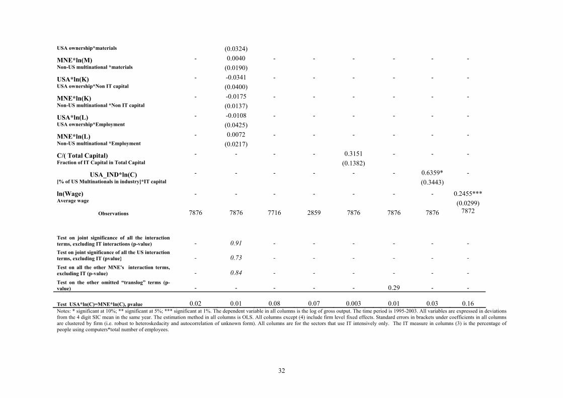
Table 2 presents a series of tests showing the robustness of the main results - we focus on the fixed

effects specification in the IT intensive sectors which are the most demanding specifications. The

first column represents our baseline results from column (7) in Table 1. Column (2) simply re-

iterates what we have already observed in Table 1 by estimating the production function with a full

set of interactions between the US dummy and all the factor inputs. None of the additional non-IT

factor input interactions are individually significant and the joint test at the base of the column of

the additional interactions shows that they are insignificant (for example the joint test of the all the

US interactions except the IT interaction has a p-value of 0.73). We cannot reject the specification

in column (1) as a good representation of the data against the more general interactive models of

11 See Appendix Table A1 for a full list, which are the same as those in Figure 2. We follow the same definitions of the sectors that intensively use IT as Van Ark et al (2002) who follow Stiroh (2002). Table A5 presents the results of the fixed effects regressions on the separately for wholesale, retail and the rest of the IT intensive sectors. 12 The p-value on the test of the coefficients US*IT = MNE*IT is 0.02 for the specification in column (7).

13

Table 1.13 If, for example, the productivity advantage of the US was due to differential mark-ups

then we would expect to see significantly different coefficients on all the factor inputs, not just on

the IT variable (Klette and Griliches, 1996).

A concern is that we may be underestimating the true IT stock of US multinationals in the initial

year generating our interaction term due to greater measurement error of IT capital for the US

establishments. We approach this issue in two ways. First, we use an alternative measure of IT

capital (built from our data using employment weights to build the initial condition for the IT

capital stocks), and we still find a positive and significant interaction (column 3). Second, we turn

to an alternative IT survey (the E-commerce Survey, described in the Appendix) that has data on the

proportion of workers in the establishment who are using computers. This is a pure “stock” measure

so is unaffected by the initial conditions concern14. In Column (4) we replace our IT capital stock

measure with this proxy. Reassuringly we still find a positive and significant US ownership

interaction. The fifth column of Table 2 implements an alternative way of examining whether the IT

productivity impact is higher for US multinationals by aggregating IT and non-IT capital into total

capital and including an additional variables for the proportion of IT capital in the total capital stock

and its interactions with the ownership dummies. All terms are positive and the US interaction with

IT is significantly different from zero at the 1% level. Another concern is that the US*IT interaction

reflects some other non-linearity in the production function. We tried including a much fuller set of

interactions and higher order terms (a “translog” specification), but these were insignificant.

Column (6) shows the results of including all the pairwise interactions of materials, labour, IT

capital and non-IT capital and the square of each of these factors. The additional terms are jointly

insignificant (p-value = 0.29) and the US interaction with the linear IT term remains basically

unchanged. Column (7) presents a value added based specification instead of an output based

specification. The results are similar to using gross output (although the coefficients are larger of

course).

13 We also investigated whether the coefficients in the production function regressions differ by ownership type and sector (IT intensive or not). Running the 6 separate regressions (3 ownership types by two broad sectors) we found the F-test rejected at the 1% pooling of the US multinationals with the other firms in the IT intensive sectors. In the non-IT intensive sectors, by contrast, the pooling restrictions were not rejected. Details on request from the authors. 14 Our IT stock measure is more appropriate theoretically as it is built in an entirely analogous way to the non-IT stock and comparable to best practice existing work. The E-Commerce Survey is available for three years (2001 to 2003), but the vast majority of the sample is observed only for one period, so we do not control for fixed effects.

14

Another possible explanation for the higher productivity of IT in US firms is that US multinationals

may be disproportionately represented in specific industries in which the IT coefficient is

particularly high. The interaction of IT capital with the US dummy would then capture omitted

industry characteristics rather than a “true” effect linked to US ownership. To test for this potential

bias we included in our regression as an additional control the percentage of US multinationals in

the specific four-digit industry (“USA_IND”)15. We also construct a similar industry level variable

for the non-US multinationals (“MNE_IND”). The IT elasticity is higher in sectors with a larger US

MNE presence (see column (8)) and this is significant at the 10% level, but the coefficient on the

IT*US interaction remains largely unchanged. Next, we considered the role of skills. Our main

control for labour quality in Table 1 is the inclusion of establishment specific fixed effects which,

so long as the labour quality does not change too much over time, should control for the omitted

human capital variable. As an alternative, we assume that wages reflect marginal products of

workers so that conditioning on the average wage in the firm is sufficient to control for human

capital16. The average wage is highly significant, but the interaction between the average wage and

IT capital was positive but insignificant. The interaction between the US dummy and average wages

in the plant were also insignificant (p-value =0.512)17.

We also implemented a large number of other robustness tests including alternative econometric

estimation techniques, different versions of dealing with measurement error in the capital stocks and

more flexible specifications of the production function. One issue is that US firms may be more

productive in the UK because the US is geographically further away than the other multinationals

(mainly European countries) and only the most productive firms are able to overcome the fixed

costs of distance. To test this we divided the non-US multinational dummy into European vs. non-

European firms. Under the distance argument, the non-European firms would have to be more 15 The variable is constructed as an average between 1995 and 2003 and is built using the whole ARD population. 16 The problem is that wages may control for “too much” as some proportion of wages is almost certainly related to other factors apart from human capital. For example, in many models, firms with high productivity will reward even homogenous workers with higher wages (see Van Reenen (1996) on rent sharing). 17 As an alternative we matched in education information at the industry-region level from an individual level survey, the Labor Force Survey. In the specifications without fixed effects, there was some evidence for a positive and significant interaction between skills and IT consistent with complementarity between technology and human capital. The US*IT capital interaction remained significant. Including fixed effects, however, renders the skills variables and

15

productive to be able to set up plant in the UK. In the event, the European and non-European

multinationals were statistically indistinguishable from each other – it was again the US

multinationals that appeared different18. We were also concerned that the US firm advantage may

simply be due to their larger size. We did not find that the US firms were larger at the median

compared to non-US multinationals, however. Furthermore, interactions of total firm (or total

establishment) size with IT were insignificant.

IV.C. US Multinational Takeovers of UK establishments

One possible explanation for our results is that US firms “cherry pick” the best establishments with

the highest potential productivity impact from IT. This would generate the positive interaction we

find but it would be entirely due to selection on unobserved heterogeneity rather than higher IT

productivity due to US ownership. To look at this issue we examined the sub-sample of

establishments who were, at some point in our sample period taken over by another firm,

considering both US and non-US acquirers. Because of the high rate of M&A activity in the UK,

this is a large sample (5,718 observations). In columns (1) and (2) of Table 3 we start by estimating

our standard production functions (with and without IT respectively) for all establishments that are

eventually taken over in their pre-takeover years (this is labeled “before takeover). The coefficients

on the observable factor inputs are very similar to those for the whole sample in columns (1) and (2)

of Table 1. Unlike the full sample, however, the US and non-US ownership dummies are also

insignificant, suggesting the establishments that multinationals take over are not ex ante more

productive than those acquired by domestic UK firms.

In column (3) of Table 3 we interact the IT capital stock with a US and a non-US multinational

ownership dummy, again estimated on the pre-takeover data. We see that neither interaction is

significant – that is before establishments are taken over by US firms they do not show a

their interactions insignificant (even though US*IT interaction remains significant). Interactions between the US dummy and skills were insignificant in all specifications. 18 In specifications of column (2) Table 1 the European dummy was 0.042 compared to 0.040 for the non-European, non-US multinational dummy (the US dummy was 0.075). All were significantly more productive than domestic establishments. The interactions of these extra dummies with IT capital were always insignificant (e.g. In the specification of Table 1 column (3) the coefficient on the non-US non-EU multinational interaction with IT capital was 0.006 with a standard error of 0.006 whereas the US interaction was 0.011 with a standard error of 0.005).

16

significantly higher IT productivity impact. So, US firms also do not appear to be selecting

establishments which provide a higher IT productivity. In columns (4) and (5) we run a similar

production function check on the post-takeover sample and again observe very similar coefficients

to columns (1) and (2) in Table 1, suggesting that these post takeover establishments are also

similar to the rest of the sample. This time, however, the non-US and US multinational ownership

coefficients are positive and significant. Thus, a transfer of ownership from domestic to

multinational production is associated with an increase in productivity, particularly for a move to

US ownership.

Column (6) is a key result for Table 3. It estimates a specification allowing the IT capital stock

coefficient to vary by ownership for the post takeover sample. In this group we do indeed see a

higher IT productivity impact for US firms, which is significant at the 10% level, but not for non-

US owned establishments. Hence, after a takeover by a US MNE establishments significantly

increase their IT productivity impact, but not after a takeover by a non-US MNE. The inclusion of

this US interaction also drives the coefficient on the linear US multinational term into

insignificance, suggesting the main reason for the improved performance of establishments after a

US takeover is linked to the increased IT productivity.

The final column of Table 3 breaks down the post takeover period into the first year after the

takeover and the subsequent years (throughout the table we drop the takeover year itself as there is

likely to be restructuring in that period). The greater productivity of IT capital in establishments

taken over by US multinationals is only revealed two and three years after takeover (the interaction

is significant at the 5% level whereas the interaction in after the first year is insignificant). This is

consistent with the idea that US firms take a couple of years to get the organizational capital of the

firm in place before obtaining higher productivity gains from IT. Domestic and other multinationals

again reveal no pattern with all dummies and interactions remaining insignificant.

Table 4 explores this idea further by running IT investment equations for the establishments that

have been taken over at some point. The first column focuses on the pre-takeover period and shows

that the establishments who were subsequently taken over by US firms were no more IT intensive

than other establishments taken over by non-US multinationals or domestic UK firms. The second

17

column contains the results from the post-takeover period. Again, there is evidence that US

establishments invest significantly more in IT than other statistically similar establishments taken

over by other firms. The final column splits the takeover period into the first year post-takeover and

then the second and third. As with productivity, the boost to IT in US takeovers takes more than just

one year to occur with the increase in IT capital being a gradual process.

As another cut on the cherry-picking concept we ran a probit of US takeovers where the dependent

variable is equal to unity for establishments who are taken over by a US firm and otherwise. We

find that IT intensity is insignificant in this regression. Hence, US firms do not appear to target

establishments that are particularly IT intensive prior to the takeover, but instead increase the IT

intensity of these establishments post-takeover. 19

Finally Table 5 investigates a little further the sectors driving the higher returns to IT for US firms

in the IT intensive sector by breaking out its two largest sectors groups – Retail and Wholesale - and

comparing these to the remaining sectors. In column (1) we simply represent the results from

column (7) in table 1 to provide the baseline of all IT intensive sectors. In columns (2), (3) and (4)

we see that the coefficients on the US interaction are remarkably similar across Retail, Wholesale

and all other IT intensive sectors. It also highlights the role that Retail and Wholesale play given

their large share of total output in the IT intensive sector.

IV.D. Further Investigations

Could the higher IT coefficient simply be due to greater software intensity in US firms? We have

some information of software expenditure that we can use to build analogous measures of the

software IT stock. When included in the specifications these stocks are positive and significant, but

the hardware coefficient is only slightly reduced. Using the same specification as Table 1 column

(2) when the software stock is included it has a coefficient of 0.0138 and a standard error of 0.0038.

Conditional on this software stock the hardware coefficient is 0.0284 with a standard error of

0.0049. The hardware interaction with the US remains positive and significant when software is

included. For example in column (3) of Table 1 the hardware interaction has a coefficient of 0.0.370

19 After a take-over by a US multinational establishments increase their IT capital per head by 30%, which is significantly different from takeovers by non-US multinational establishments at the 5% level.

18

with a standard error of 0.0166. One concern with comparing software data for multinationals

versus domestic firms may be that some multinational software development happens in the home

country, which is not fully measured through transfer pricing, so that multinational subsidiary

software expenditure under-reports total software inputs. This emphasizes the importance, however,

of comparing US multinationals to non-US multinationals that should have similar “underreporting”

issues to the extent these occur. As noted above, whether or not we include these software

measures, US multinationals still obtain a significantly higher productivity from IT inputs than

either domestic firms or other non-US multinationals.

V. A SIMPLE THEORETICAL MODEL OF IT AND PRODUCTIVITY

In this section we consider a formal model that can rationalize the macro stylized facts and the

results that we see in the empirical analysis. We base this theory on the costs of making

organizational changes as this seems to be consistent with a range of information from case studies

and other papers. We readily concede that this is not the only model that could rationalize some of

the facts (see sub-section V.B below), but we think that it is a compelling model to fit the general

facts in our empirical study and the more general literature.

V.A. Basic Model

Consider two representative firms, one in the US and one in the EU. To keep things as simple as

possible we assume that technology, prices and all parameters (except organizational adjustment

costs) are globally common in the two regions. Firms in the US and EU are always optimizing - i.e.

European firms are not making systematic “mistakes” by choosing a different organizational form,

but reacting optimally given their different adjustment costs.

The firms produces output (Q) by combining IT (C) inputs, non-IT physical capital inputs (K) and

labor inputs (L), with all other inputs assumed zero for simplicity, and is defined as follows:

Q = A Cα+σO Kβ -σO L1-α-β

19

Organizational structure is denoted O and is normalized on a scale from zero as Taylorist

“centralized” production to unity as modern re-organized (or “decentralized”) production20. The α,

β and σ are production function parameters where 0 < α+ β < 1 and 0 < σ < β. This specification of

the production function is a simple way of capturing the notion that IT and re-organized production

are complementary as σ > 0.21 Second, we have modeled O as having only adjustment costs, there is

no “price” of a level of organizational capital nor is there always a positive marginal product of

output with respect to O. This implies that the optimal organizational form will depend on the

relative prices of the factor inputs and technology. In earlier eras the higher price of IT meant that

firms were more intensive in physical capital (K), which gave no advantage to positive levels of O.

The firm sells its output into a market with iso-elastic demand elasticity e ( >1) so that P = BQ-1/e

where P is the output price and B is a demand shock parameter.

Combining the production and demand functions together we can write revenue as

PQ = Z(Cα+σO Kβ -σO L1-α-β) 1 -1/e

where Z = BA1-1/e is an arbitrary constant (since A and B are arbitrary sizing constants), defining

ω = α(1-1/e), µ= β(1-1/e), γ = (1-α- β)(1-1/e) and λ = σ(1-1/e) we combine together the production

function parameters and the demand parameters to re-write revenue as22

γλµλω LKCPQ OO −+=

Flow profits can then be defined as follows:

20 We choose centralization/decentralization based on some of the case study evidence, but to some extent this is just labelling. What matters is that the optimal organizational form changes with IT and that there are costs associated with making this change. 21 The restriction that σ > 0 does not guarantee that C and O will be Hicks-Allen complements, but it certainly makes this more likely. Although we label O as an index of decentralization it obviously captures a much broader notion of organization that are better for increasing the relative productivity of IT. 22 For simplicity we have not allowed O to also enter in the exponent of L. Nothing fundamental would change from allowing– what matters is the strength of the positive interaction between lnC and O is stronger than it is with the other two factors.

20

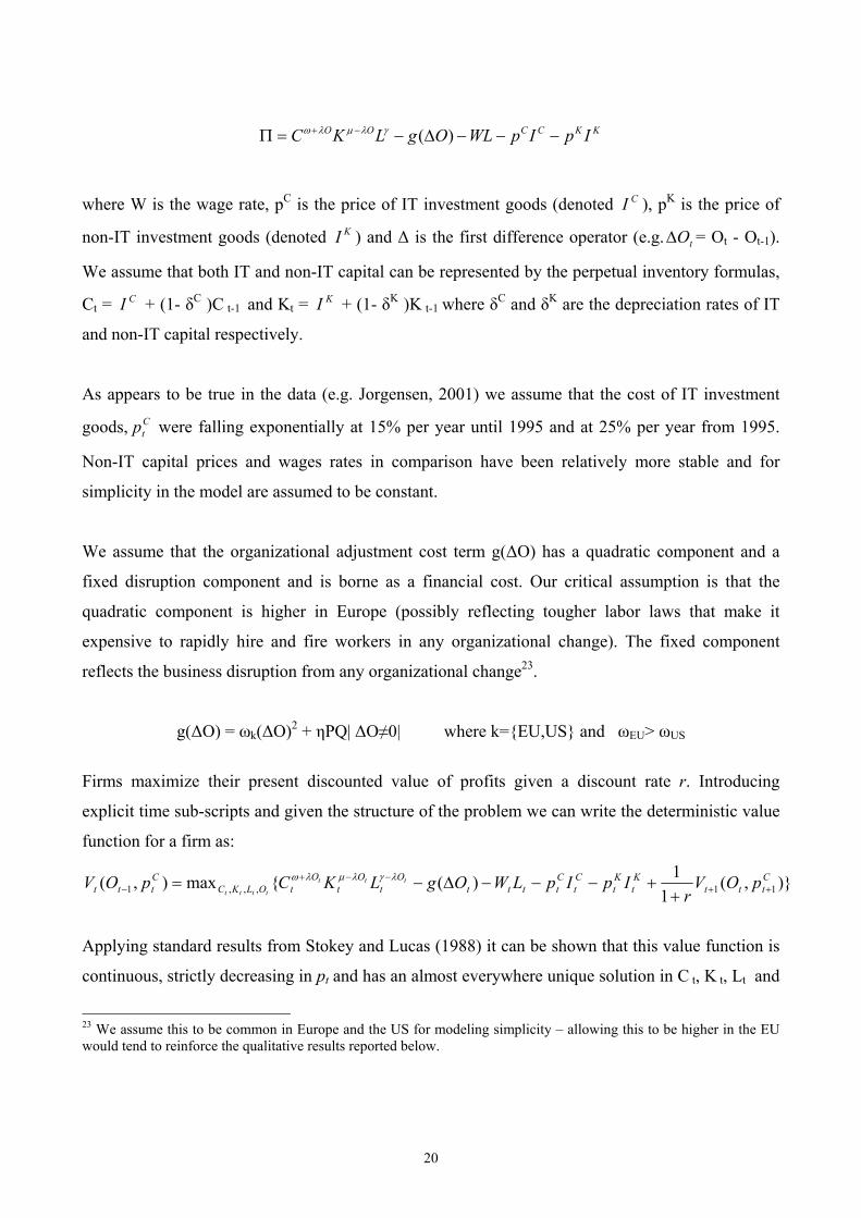
KKCCOO IpIpWLOgLKC −−−∆−=Π −+ )(γλµλω

where W is the wage rate, pC is the price of IT investment goods (denoted CI ), pK is the price of

non-IT investment goods (denoted KI ) and ∆ is the first difference operator (e.g. tO∆ = Ot - Ot-1).

We assume that both IT and non-IT capital can be represented by the perpetual inventory formulas,

Ct = CI + (1- δC )C t-1 and Kt = KI + (1- δK )K t-1 where δC and δK are the depreciation rates of IT

and non-IT capital respectively.

As appears to be true in the data (e.g. Jorgensen, 2001) we assume that the cost of IT investment

goods, Ctp were falling exponentially at 15% per year until 1995 and at 25% per year from 1995.

Non-IT capital prices and wages rates in comparison have been relatively more stable and for

simplicity in the model are assumed to be constant.

We assume that the organizational adjustment cost term g(∆O) has a quadratic component and a

fixed disruption component and is borne as a financial cost. Our critical assumption is that the

quadratic component is higher in Europe (possibly reflecting tougher labor laws that make it

expensive to rapidly hire and fire workers in any organizational change). The fixed component

reflects the business disruption from any organizational change23.

g(∆O) = ωk(∆O)2 + ηPQ| ∆O≠0| where k=EU,US and ωEU> ωUS

Firms maximize their present discounted value of profits given a discount rate r. Introducing

explicit time sub-scripts and given the structure of the problem we can write the deterministic value

function for a firm as:

),(1

1)(max),( 11,,,1Cttt

Kt

Kt

Ct

Ctttt

Ot

Ot

OtOLKC

Cttt pOV

rIpIpLWOgLKCpOV ttt

tttt ++−−+

− ++−−−∆−= λγλµλω

Applying standard results from Stokey and Lucas (1988) it can be shown that this value function is

continuous, strictly decreasing in pt and has an almost everywhere unique solution in C t, K t, Lt and

23 We assume this to be common in Europe and the US for modeling simplicity – allowing this to be higher in the EU would tend to reinforce the qualitative results reported below.

21

Ot. Given any initial conditions for Cp0 and O0 the policy correspondence functions can be used

iteratively to solve the time path of Ct, K t, Lt and Ot .

The long-run qualitative features are reasonably obvious. As the price of IT continues to fall the

steady state optimal organizational form is complete decentralization for all firms (O equal to

unity). The interesting question, however, is the transitional dynamics and how this differs between

the US and Europe. Although the model has a well-behaved analytical solution in order to derive

numerical values for any particular set of parameter values, however, we need to use numerical

methods.

To do this we defined the parameter values as follow. We set: α = 0.025 reflecting a 2.5% revenue

share for IT, β = 0.3 reflecting a 30% revenue share for non-IT capital, and e = 3 reflecting a 50%

mark-up over marginal costs, mc, ((P-mc)/mc = 1/(1-e)). The parameter λ has no obvious value, so

we set this at λ = ω so that full “decentralization” (moving from O equal zero to O equal unity)

doubles the value or the marginal product of IT and reduces the value of the marginal product of

capital by just under 10% . Picking larger or smaller values of λ while holding the scaling on O

constant increases or reduces the degree of complementarity between O and λ. The discount rate is

set at r = 10%, the IT depreciation rate at δC = 30% (Basu et al, 2003), the non-IT depreciation rate

of δK = 10% and the wage rate is normalized to unity (W = 1). The fixed cost of adjustment are set

at η = 0.2 percent of sales selected on the evidence for the fixed costs of capital investments (see

Bloom, 2006) given the lack of any direct evidence on the cost of organizational adjustment costs.

The quadratic adjustment cost parameter is set so adjustment costs are four times as high in Europe

as in the US (i.e. ωUS/ωEU = 4, roughly similar to the differences in the OECD’s labor regulation

indices in Nicoletti et al, 2000). The starting values for Cp0 and O0 are taken as Cp0 = 0.075 and O0

= 0 in 1965, with the price process then exponentially decaying (as outlined above) until 2025 at

which point prices stop falling any further. The first and last ten years of the simulation are then

discarded to abstract from any initial and terminal restrictions24.

24 The code is written in MATLAB and is available on request from the authors.

22

The model has several intuitive predictions that are consistent with the stylized facts and also

contains some novel predictions. First, we trace out the decentralization decisions of firms in Figure

6. We see that US firms start to decentralize first (in the late 1980s in the baseline case) and are on

average more decentralized than European firms throughout the period under consideration (the

representative EU firm begins to decentralize about 19 years after the American firm). The US

decentralizes first because of its lower adjustment costs. The fixed costs implies that firms always

change O in discrete “chunks” and the cost of making any given jump will always be greater for

European firms because of their higher adjustment costs25.

Figure 7 examines the pattern of IT per unit of capital in logarithms (ln(C/K)). Unsurprisingly this

is rising in both regional blocs due to the global fall in IT prices. IT intensity grows at an identical

rate in the two regions until the US starts to decentralize and at this point American firms start to

become more IT intensive than European firms. This is because of the complementarity underlying

the production function (higher O implies higher optimal IT investment). Labour productivity

(Q/L) is shown in Figure 8. Unsurprisingly, the higher IT intensity translates through into higher

labor productivity which accelerates from the mid 1990s.

These findings are consistent with the broad macro facts as discussed earlier. We now discuss

extensions to fit the micro data results.

V.B. Extensions to the basic model

(a) Multinationals

We now consider multinational companies who operate several plants at least one of which is on

foreign soil. We extend the modeling framework to consider an additional cost in maintaining

different organizational forms in different plants. Multinationals appear to operate globally similar

management and organizational structures (e.g. Bartlett and Ghoshal, 1999) as this makes it much

easier to integrate senior managers, human resource systems, software, etc. At different ends of the

25 Without any fixed costs, O will be changed in infinitesimally small increments due to the quadratic adjustment costs. In this case the higher quadratic adjustment costs of European firms gives them an incentive to smooth adjustment more than US firms which will mean that European firms start to decentralize first. In the limit when US adjustment costs are zero, US firms will adjust in a single period when optimal C/K = 1. Before this point European firms will be more decentralized, more IT intensive and have higher labor productivity. After this point the opposite is true. This shows the importance of allowing for fixed adjustment costs in matching the stylized facts.

23

skills spectrum both McKinsey and Starbucks are recognizably similar in Cambridge,

Massachusetts and Cambridge, England. To formalize this we allow an additional quadratic

adjustment cost which has to be born if there is a difference between the organization of the plant i

(Oi) and its parent ( kO ), ik

i PQOO )()( 2−φ

Consider the case of a US firm purchasing a European plant (in the period after US firms have

started to decentralize). The purchased plant will start to become more decentralized than identical

plants owned by domestic firms (or European multinationals operating solely in Europe). It will

also start increasing IT intensity and labor productivity at a faster rate than European owned plants.

The degree to which the plant resembles its American parent will depend on the size of φ relative

to the adjustment cost differential EUω . The larger is φ the more the establishment will start to

resemble its US parent26. Note that the presence of adjustment costs, however, suggests that this

change will not be immediate so after an American firm takes over a European establishment the IT

intensity and productivity will be, for some periods, below than of longer-established US affiliates.

The middle line in Figure 9 shows the simulation results for a hypothetical British plant taken over

by a US multinational in 2003. The calibration assumes iφ =1. Under this scenario, the taken over

firm initially converges to within 0.1 of the organizational structure of the US parent company five

years after the take over year.

These are the key testable predictions that we take to the micro data – is it the case that US

multinationals not only perform more IT than EU multinationals but also appear to obtain higher

productivity from their IT capital stock? When US firms takeover European establishments do we

see these patterns emerge in the data?

(b) Industry Heterogeneity

26 This raises questions about the reasons for takeovers. Why should a US firm ever take over a European plant if it has to bear greater adjustment costs than a European multinational? One reason is that the US parent may have higher TFP from some firm-specific advantage that it can diffuse to the affiliate (such as better technology or management).

24

The fall in the price of IT has opened up the possibility of IT-enabled innovations to a greater extent

in some industries than others. Baker and Hubbard (2004) for example describe how on-board

computers have altered business methods in the trucking industry. In our model we can capture this

by allowing a different degree of complementarity between IT and organization in some industries

than others (i.e. a higher σ). Those sectors in Figure 2 that Stiroh and others have labeled “intensive

in IT using” would have a higher σ and therefore follow the patterns analyzed above. Other sectors

with low σ would not and for these industries US and EU productivity experience should be similar

as both regions enjoy the benefits of faster productivity growth. This is what we find in the micro

data – the differences between US and EU firms are much stronger in the intensive IT using sectors.

(c) Adjustment Costs for IT capital

For simplicity we abstracted away from adjustment costs in IT capital and other factors of

production. Consider a simple extension of the model where we also have quadratic adjustment

costs in IT capital, but assume that these are the same across countries. Obviously this will slow

down the accumulation of IT and O, but the qualitative findings discussed above will still go

through27. One difference, however, is that measured TFP will grow more quickly in the US than in

the EU as decentralization occurs under this model. Under the baseline model the share of IT capital

in revenue is still equal to Oλω + in every period so the “weight” on IT capital in the measured

TFP formula will be correct. Once we allow for adjustment costs in IT, by contrast, the empirical

share of IT in revenues will always be below its steady state level (in the period when O is greater

than zero and less than unity). This will mean that measured TFP will exceed actual TFP (A) and

that measured TFP in the US will exceed that of the EU in the transition.

(d) Permanent Differences in Management Quality?

An alternative model to the one we have presented could be one were US firms have always been

better managed/organized than European firms and that this better management is complementary

with IT. This could be due to tougher competition, culture, less family run firms, etc. Under this

27 For an analysis of mixed fixed and quadratic adjustment costs with two factors see Bloom, Bond and Van Reenen (2006) or Bloom (2006).

25

model “O” would enter as an additional factor input in the production function with an exogenously

lower price in the US than in Europe. For example,

Q = A OχCα+σO Kβ -σO L1-α-β-χ

This set-up would rationalize most of the findings presented in the paper except one. We found in

Table 1 and elsewhere that the linear US multinational dummy was insignificantly different from

zero once we have accounted for the higher coefficient on IT capital for US firms. In the extended

equation above, then, we find σ>0 but χ = 0. Consequently, we have some preference for the more

parsimonious model presented here. It is the flexibility of the US economy in adapting to the

challenges of major changes (such as the IT revolution) that gives it productivity advantage, not its

permanent superiority in all states of the world. Of course, if we have moved into a stage of

development where turbulence is inherently greater, then the US will retain an edge over Europe for

the foreseeable future.

VI. CONCLUSIONS

Using a large and original establishment level panel dataset we find robust evidence that IT has a

positive and significant correlation with productivity even after controlling for many factors such as

fixed effects. We estimate that a doubling of the IT stock is associated with an increase in

productivity of between 2% and 4%. The most novel result is that we can account for the US

multinational advantage in conventionally measured TFP by their higher productivity impact of IT

capital. Furthermore, the stronger association of IT with productivity for US firms is confined to the

same “IT using intensive” industries that largely accounted for the US “productivity miracle” since

the mid 1990s. US firms in the UK were able to get significantly more productivity out of their IT

than other multinational (and domestic British) firms, even in the context of a UK environment.

This suggests that part of the IT-related productivity gains in the US may be due to the

management/organizational capital of firms rather than simply the “natural advantages”

(geographical, institutional or otherwise) of the US environment.

26

A major research tasks remain in understanding why US firms are able to achieve these “IT

friendly” organizational forms and their European counterparts cannot. It could be due to timing –

US firms where closer to the development of the new wave of IT producers and so were the first to

learn about them. In this scenario European firms will quickly catch up (although there is little

evidence of this happening so far). A second explanation is that US firms are “leaner and meaner”

than their European counterparts due to tougher competitive conditions in their domestic markets

and are therefore intrinsically quicker to adapt to revolutionary new technologies. Alternatively, US

firms may be more organizationally devolved for historical reasons due to their greater supply of

college levels skills, relative absence of family owned firms and/or their history of technological

leadership (see Acemoglu et al, 2006), rendering them better equipped to adopt new IT

technologies. Under these scenarios Europe will resume the catching up process with a much longer

lag than is conventionally thought.

27

REFERENCES

Acemoglu, D., Aghion, P., Lelarge, C., Van Reenen, J. and Zilibotti, F. (2005) “Technology, Information and the Decentralization of the firm”, LSE mimeo Arellano, M. and Bond, S. (1991), “Some tests of specification for panel data: Monte Carlo evidence and an application to employment functions”, Review of Economic Studies, 58, 277-297 Bartlett and Ghoshal (1999) Managing Across Borders: The Transnational Solution, Harvard: Harvard University Press Baker, George and Thomas Hubbard (2004) “Contractability and Asset Ownership: On board computers and governance in US trucking” Quarterly Journal of Economics, 119, 1443-79 Basu, Susanto, Fernald, John G., Oulton, Nicholas, Srinivasan, Sylaja (2003) “The Case of the Missing Productivity Growth: Or, Does information technology explain why productivity accelerated in the United States but not the United Kingdom?” NBER Macro-economics Annual Blanchard, Olivier (2004) “The Economic Future of Europe” Journal of Economic Perspectives, 18,4, 3-26 Bloom, Nick (2006) “The Impact of Uncertainty shocks: Firm level estimation and a 9/11 Simulation” Centre for Economic Performance Working Paper No. 12383 Bloom, Nick and Van Reenen, John (2006), “Measuring and explaining management practices across firms and countries”, Centre for Economic Performance Working Paper No. 716 Bloom, Nick, Bond, Steve and Van Reenen, John (2006) “Uncertainty and company investment dynamics: Empirical Evidence for UK firms” NBER Discussion Paper Blundell, Richard and Bond, Steve (1998) “Initial Conditions and Moment Restrictions in dynamic

panel data models” Journal of Econometrics, volume 88, 115-143. Blundell, Richard and Bond, Steve (2000) “GMM Estimation with persistent panel data: an

Application to production functions” Econometric Reviews, 19(3), 321-340. Bresnahan, Tim, Brynjolfsson, Erik and Hitt, Lorin (2002) “Information Technology, Workplace Organization and the Demand for skilled labor” Quarterly Journal of Economics, 117(1), 339-376 Brynjolfsson, Erik and Hitt, Lorin (2000) “Beyond Computation: Information Technology, Organisational Transformation and Business Performance.” Journal of Economic Perspectives, Vol. 14 No. 4, 23-48

Brynjolfsson, Erik Hitt, Lorin and Yang, Shinkyu (2002) “Intangible Assets: Computers and Organizational Capital.” MIT Sloan, Paper 138

28

Brynjolfsson, Erik and Hitt, Lorin (2003) “Computing Productivity : Firm Level Evidence” Review of Economics and Statistics, 85 4, 793-808 Caroli, Eve, and Van Reenen, J. (2001) “Skill biased organizational change? Evidence from British and French establishments" Quarterly Journal of Economics CXVI, No. 4, 1449-1492 Chennells, Lucy, and John Van Reenen, ” (2002) “The effects of technical change on skills, wages and employment: A Survey of the Micro-econometric evidence” Chapter 5 in L’Horty, Y. and Greenan, N., and Mairesse, J. Productivity, Inequality and the Digital Economy MIT Press 175-225

Colecchia, A. and Schreyer (2002) “ICT Investment and Economic Growth in the 1990s : Is this United States a Unique Case ? ” Review of Economic Dynamics, 408-442

Crepon, B. and Heckel, T. (2002) “Computerization in France : an Evaluation based on individual company data” Review of Income and Wealth, 1, 1-22

Criscuolo, Chiara and Martin, Ralf (2004) “Multinationals and US Productivity Leadership: Evidence from Great Britain” ,Centre for Economic Performance Discussion Paper No. 672 Doms, M., Dunn, W., Oliner, S., Sichel, D. (2004) ”How Fast Do Personal Computers Depreciate? Concepts and New Estimates ”, NBER Working Paper No. 10521 Doms, M. and Jensen, J. (1998) “Comparing Wages, skills and productivity between domestically owned manufacturing establishments in the United States” in Robert Baldwin, R.E.L. and Richardson,. (eds) Geography and Ownership as bases for economic accounting, 235-258, Chicago: University of Chicago Feenstra, R. and Knittel, C. (2004) “Re-assessing the US quality adjustment to computer prices: The role of durability and changing software” NBER Working Paper 10857 Geske, Ramey and Shapiro (2004) “Why do computers depreciate?” NBER Working Paper 10831 Gordon, R. (2004) “Why was Europe left at the station when America’s Productivity Locomotive departed?” NBER Working Paper No. 10661 Griffith, R., Simpson, H. and Redding, S. (2002) “Productivity Convergence and Foreign Ownership at the Establishment Level ” Centre for Economic Policy Research Discussion Paper No. 2765 Griliches, Zvi, and Jacques Mairesse (1998) "Production functions: The Search for Identification" in Scott Ström (ed.), Essays in Honour of Ragnar Frisch, Econometric Society Monograph Series, (Cambridge: Cambridge University Press, 1998). Haltiwanger, J., Jarmin, R. and Schank, T. (2003) “Productivity, Investment in ICT and market experimentation: Micro evidence from Germany and the U.S” Center for Economic Studies Discussion Paper 03-06

29

Klette, Tor Jakob (1999) “Market power, scale economies and productivity: Estimates from a panel of establishment data”, Journal of Industrial Economics, 47, 451-76. Klette, Tor and Griliches, Zvi (1996) “The inconsistency of Common Scale estimators when output prices are unobserved and endogenous” Journal of Applied Econometrics, 11, 343-361

Jorgenson, Dale and Stiroh, Kevin (2000) “Raising the Speed Limit: US Economic Growth in the Information Age.” Brookings Papers on Economic Activity, 1 :125-211 Jorgenson, D. W. (2001) “Information technology and the U. S. economy”, American Economic Review, 91(1), 1-32.

Nicoletti, Giuseppi, Scarpetta, Stefano and Boyland, O. (2000) “Summary Indicators of Product Market Competition with an extension to Employment Protection” OECD Working Paper No. 226, OECD: Paris Oliner, Stephen and Sichel, Daniel (2000). “The resurgence of growth in the late 1990s: is information technology the story? ” Journal of Economic Perspectives, 14(4), 3-22 Oliner, Stephen and Sichel, Daniel (2005). “The resurgence of growth in the late 1990s: Update” , mimeo Federal Reserve Bank, Washington

Olley, G. Steven, Pakes, Ariel (1996) “The Dynamics of Productivity in the Telecommunications Industry.” Econometrica Vol. 64, No. 6, 1263-1297 O'Mahony, Mary and van Ark, Bart, eds. (2003), EU Productivity and Competitiveness: An Industry Perspective Can Europe Resume the Catching-up Process?, Office for Official Publications of the European Communities, Luxembourg, 2003. Stiroh, Kevin (2002), “Information Technology and the U.S. Productivity Revival: What Do the Industry Data Say?”, American Economic Review, 92(5), December, 1559-1576. Stiroh, Kevin, (2004) “Reassessing the Role of IT in the Production Function: A Meta analysis”, mimeo, Federal Reserve Bank of New York Stokey, N., Lucas, R. and Prescott, E. (1988) Recursive Methods in Economic Dynamics, Harvard: Harvard University Press

Van Ark, Bart, Inklaar, Robert, and McGuckin Robert H. (2002) “’Changing Gear.’ Productivity, ICT and Service Industries: Europe and the United States.” Research Memorandum GD-60 University of Groningen , Groningen Growth and Development Centre Van Reenen, J (1996) “The Creation and Capture of Economic Rents: Wages and Innovation in a Panel of UK Companies” Quarterly Journal of Economics (February 1996) CXI, 443, 195-226

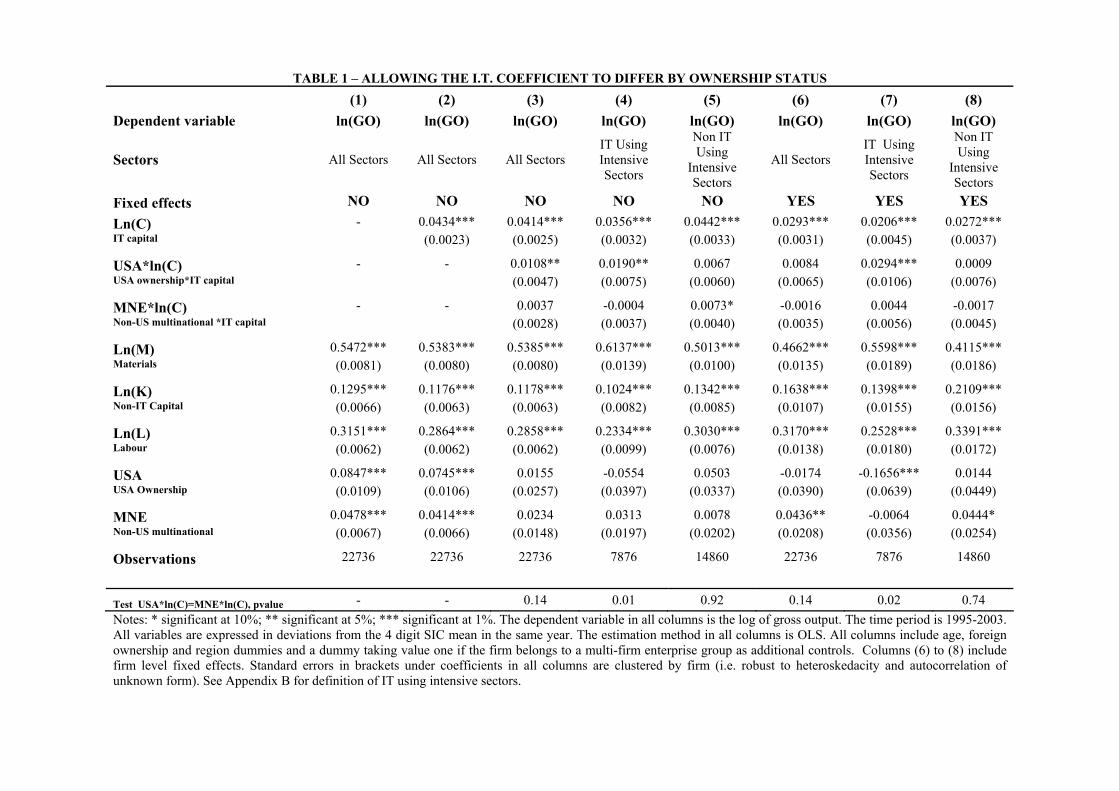
Notes: * significant at 10%; ** significant at 5%; *** significant at 1%. The dependent variable in all columns is the log of gross output. The time period is 1995-2003. All variables are expressed in deviations from the 4 digit SIC mean in the same year. The estimation method in all columns is OLS. All columns include age, foreign ownership and region dummies and a dummy taking value one if the firm belongs to a multi-firm enterprise group as additional controls. Columns (6) to (8) include firm level fixed effects. Standard errors in brackets under coefficients in all columns are clustered by firm (i.e. robust to heteroskedacity and autocorrelation of unknown form). See Appendix B for definition of IT using intensive sectors.

TABLE 1 – ALLOWING THE I.T. COEFFICIENT TO DIFFER BY OWNERSHIP STATUS

(1) (2) (3) (4) (5) (6) (7) (8) Dependent variable ln(GO) ln(GO) ln(GO) ln(GO) ln(GO) ln(GO) ln(GO) ln(GO)

Sectors All Sectors All Sectors All Sectors IT Using Intensive Sectors

Non IT Using

Intensive Sectors

All Sectors IT Using Intensive Sectors

Non IT Using

Intensive Sectors

Fixed effects NO NO NO NO NO YES YES YES Ln(C) - 0.0434*** 0.0414*** 0.0356*** 0.0442*** 0.0293*** 0.0206*** 0.0272*** IT capital (0.0023) (0.0025) (0.0032) (0.0033) (0.0031) (0.0045) (0.0037)

USA*ln(C) - - 0.0108** 0.0190** 0.0067 0.0084 0.0294*** 0.0009 USA ownership*IT capital (0.0047) (0.0075) (0.0060) (0.0065) (0.0106) (0.0076)

MNE*ln(C) - - 0.0037 -0.0004 0.0073* -0.0016 0.0044 -0.0017 Non-US multinational *IT capital (0.0028) (0.0037) (0.0040) (0.0035) (0.0056) (0.0045)

Ln(M) 0.5472*** 0.5383*** 0.5385*** 0.6137*** 0.5013*** 0.4662*** 0.5598*** 0.4115*** Materials (0.0081) (0.0080) (0.0080) (0.0139) (0.0100) (0.0135) (0.0189) (0.0186)

Ln(K) 0.1295*** 0.1176*** 0.1178*** 0.1024*** 0.1342*** 0.1638*** 0.1398*** 0.2109*** Non-IT Capital (0.0066) (0.0063) (0.0063) (0.0082) (0.0085) (0.0107) (0.0155) (0.0156)

Ln(L) 0.3151*** 0.2864*** 0.2858*** 0.2334*** 0.3030*** 0.3170*** 0.2528*** 0.3391*** Labour (0.0062) (0.0062) (0.0062) (0.0099) (0.0076) (0.0138) (0.0180) (0.0172)

USA 0.0847*** 0.0745*** 0.0155 -0.0554 0.0503 -0.0174 -0.1656*** 0.0144 USA Ownership (0.0109) (0.0106) (0.0257) (0.0397) (0.0337) (0.0390) (0.0639) (0.0449)

MNE 0.0478*** 0.0414*** 0.0234 0.0313 0.0078 0.0436** -0.0064 0.0444* Non-US multinational (0.0067) (0.0066) (0.0148) (0.0197) (0.0202) (0.0208) (0.0356) (0.0254)

Observations 22736 22736 22736 7876 14860 22736 7876 14860

Test USA*ln(C)=MNE*ln(C), pvalue - - 0.14 0.01 0.92 0.14 0.02 0.74

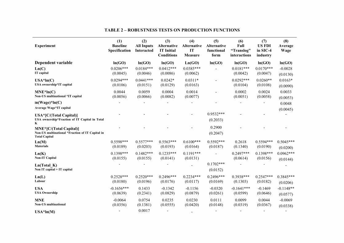
TABLE 2 – ROBUSTNESS TESTS ON PRODUCTION FUNCTIONS (1) (2) (3) (4) (5) (6) (7) (8) Experiment Baseline

Specification All Inputs Interacted

Alternative IT Initial

Conditions

Alternative IT

Measure

Alternative functional

form

Full “Translog” interactions

US FDI in SIC-4 industry

Average Wage

Dependent variable ln(GO) ln(GO) ln(GO) Ln(GO) ln(GO) ln(GO) ln(GO) ln(GO) Ln(C) 0.0206*** 0.0184*** 0.0412*** 0.0385*** - 0.0181*** 0.0170*** -0.0028 IT capital (0.0045) (0.0046) (0.0086) (0.0062) (0.0042) (0.0047) (0.0130) USA*ln(C) 0.0294*** 0.0441*** 0.0242* 0.0311* - 0.0292*** 0.0260** 0.0163* USA ownership*IT capital (0.0106) (0.0151) (0.0129) (0.0163) (0.0104) (0.0108) (0.0090) MNE*ln(C) 0.0044 0.0059 0.0004 0.0014 - 0.0002 0.0024 0.0033 Non-US multinational *IT capital (0.0056) (0.0066) (0.0082) (0.0077) (0.0051) (0.0058) (0.0053) ln(Wage)*ln(C) - - - - - - - 0.0048 Average Wage*IT capital (0.0045) USA*[C/(Total Capital)] - - - - 0.9532*** - - - USA ownership*Fraction of IT Capital in Total K

(0.2033)

MNE*[C/(Total Capital)] - - - - 0.2900 - - - Non-US multinational *Fraction of IT Capital in Total Capital

(0.2047)

Ln(M) 0.5598*** 0.5577*** 0.5563*** 0.6100*** 0.5592*** 0.2618 0.5594*** 0.5045*** Materials (0.0189) (0.0203) (0.0193) (0.0164) (0.0187) (0.1340) (0.0190) (0.0200) Ln(K) 0.1398*** 0.1482*** 0.1235*** 0.1191*** - 0.2497*** 0.1398*** 0.0962*** Non-IT Capital (0.0155) (0.0155) (0.0141) (0.0131) (0.0614) (0.0156) (0.0144) Ln(Total_K) - - - - 0.1702*** - - - Non IT capital + IT capital (0.0152) Ln(L) 0.2528*** 0.2520*** 0.2496*** 0.2234*** 0.2496*** 0.3938*** 0.2547*** 0.3845*** Labour (0.0180) (0.0196) (0.0176) (0.0117) (0.0169) (0.1303) (0.0182) (0.0206) USA -0.1656*** 0.1433 -0.1342 -0.1156 -0.0320 -0.1641*** -0.1469 -0.1148** USA Ownership (0.0639) (0.2341) (0.0829) (0.0879) (0.0261) (0.0599) (0.0646) (0.0577) MNE -0.0064 0.0754 0.0235 0.0230 0.0111 0.0099 0.0044 -0.0069 Non-US multinational (0.0356) (0.1381) (0.0555) (0.0420) (0.0148) (0.0319) (0.0367) (0.0338) USA*ln(M) - 0.0017 - - - - - -

32

USA ownership*materials (0.0324)

MNE*ln(M) - 0.0040 - - - - - - Non-US multinational *materials (0.0190)

USA*ln(K) - -0.0341 - - - - - - USA ownership*Non IT capital (0.0400) MNE*ln(K) - -0.0175 - - - - - - Non-US multinational *Non IT capital (0.0137)

USA*ln(L) - -0.0108 - - - - - - USA ownership*Employment (0.0425)

MNE*ln(L) - 0.0072 - - - - - - Non-US multinational *Employment (0.0217) C/( Total Capital) - - - - 0.3151 - - - Fraction of IT Capital in Total Capital (0.1382)

USA_IND*ln(C) - - - - - - 0.6359* - [% of US Multinationals in industry]*IT capital (0.3443)

ln(Wage) - - - - - - - 0.2455*** Average wage (0.0299)

Observations 7876 7876 7716 2859 7876 7876 7876 7872

Test on joint significance of all the interaction terms, excluding IT interactions (p-value) - 0.91 - - - - - - Test on joint significance of all the US interaction terms, excluding IT (pvalue - 0.73 - - - - - - Test on all the other MNE's interaction terms, excluding IT (p-value) - 0.84 - - - - - - Test on the other omitted “translog” terms (p-value) - - - - - 0.29 - -

Test USA*ln(C)=MNE*ln(C), pvalue 0.02 0.01 0.08 0.07 0.003 0.01 0.03 0.16 Notes: * significant at 10%; ** significant at 5%; *** significant at 1%. The dependent variable in all columns is the log of gross output. The time period is 1995-2003. All variables are expressed in deviations from the 4 digit SIC mean in the same year. The estimation method in all columns is OLS. All columns except (4) include firm level fixed effects. Standard errors in brackets under coefficients in all columns are clustered by firm (i.e. robust to heteroskedacity and autocorrelation of unknown form). All columns are for the sectors that use IT intensively only. The IT measure in columns (3) is the percentage of people using computers*total number of employees.

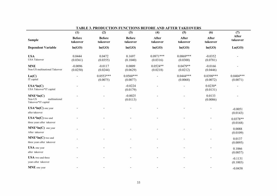
33

TABLE 3. PRODUCTION FUNCTIONS BEFORE AND AFTER TAKEOVERS

(1) (2) (3) (4) (5) (6) (7)

Sample Before takeover

Before takeover

Before takeover

After takeover

After takeover

After takeover

After takeover

Dependent Variable ln(GO) ln(GO) ln(GO) ln(GO) ln(GO) ln(GO) Ln(GO) USA 0.0444 0.0472 0.1697 0.0971*** 0.0869*** -0.0352 - USA Takeover (0.0361) (0.0355) (0.1040) (0.0316) (0.0300) (0.0781)

MNE -0.0096 -0.0117 0.0009 0.0524** 0.0479** -0.0166 - Non-US multinational Takeover (0.0250) (0.0244) (0.0629) (0.0218) (0.0212) (0.0446)

Ln(C) - 0.0553*** 0.0560*** - 0.0444*** 0.0398*** 0.0404*** IT capital (0.0075) (0.0077) (0.0068) (0.0072) (0.0071)

USA*ln(C) - - -0.0224 - - 0.0230* - USA Takeover*IT capital (0.0179) (0.0131)

MNE*ln(C) - - -0.0025 - - 0.0133 - Non-US multinational Takeover*IT capital

(0.0113) (0.0086)

USA*ln(C) one year - - - - - - -0.0051 after takeover (0.0143) USA*ln(C) two and - - - - - - 0.0378** three years after takeover (0.0168) MNE*ln(C) one year - - - - - - 0.0088 After takeover (0.0109) MNE*ln(C) two and - - - - - - 0.0137 three years after takeover (0.0095) USA one year - - - - - - 0.1066 after takeover (0.0857) USA two and three - - - - - - -0.1131 years after takeover (0.1003) MNE one year - - - - - - -0.0438

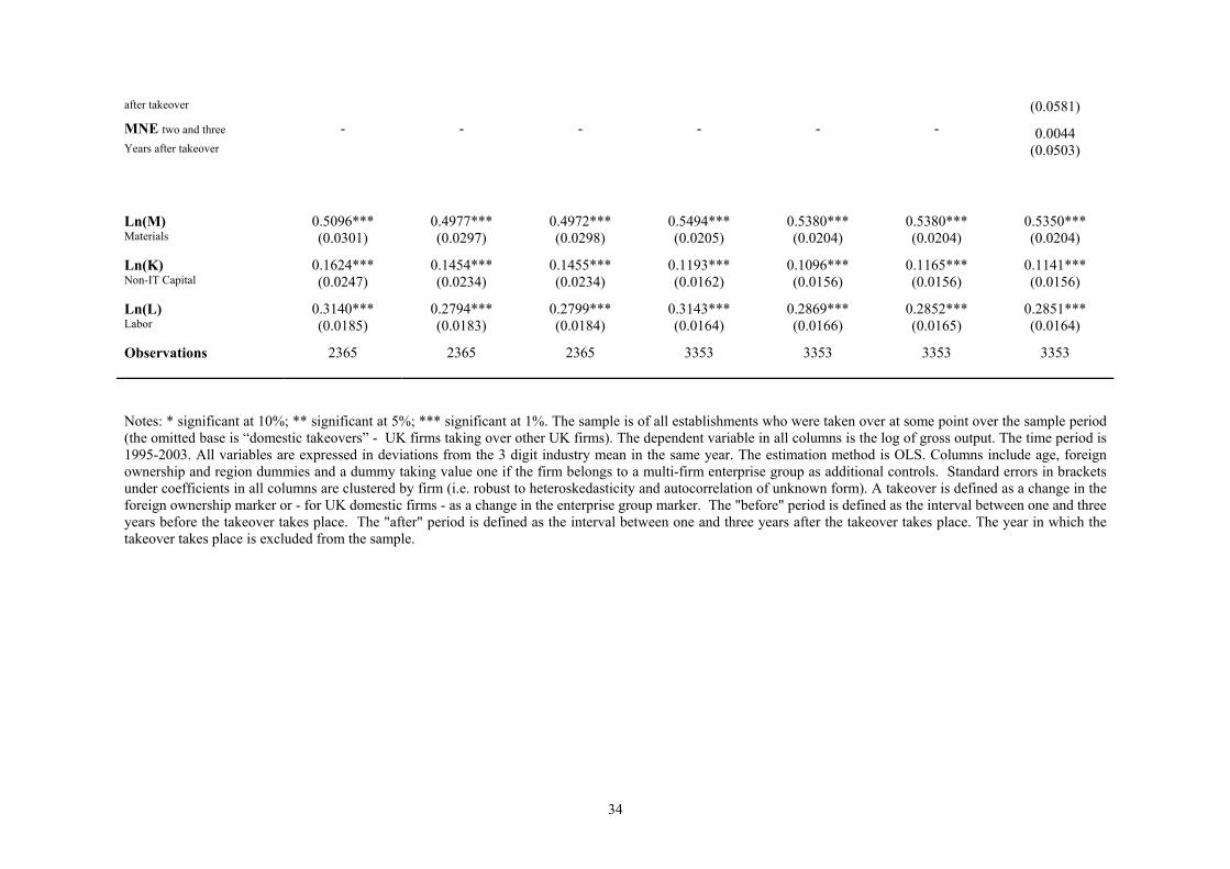
34

after takeover (0.0581) MNE two and three - - - - - - 0.0044 Years after takeover (0.0503)

Ln(M) 0.5096*** 0.4977*** 0.4972*** 0.5494*** 0.5380*** 0.5380*** 0.5350*** Materials (0.0301) (0.0297) (0.0298) (0.0205) (0.0204) (0.0204) (0.0204)

Ln(K) 0.1624*** 0.1454*** 0.1455*** 0.1193*** 0.1096*** 0.1165*** 0.1141*** Non-IT Capital (0.0247) (0.0234) (0.0234) (0.0162) (0.0156) (0.0156) (0.0156)

Ln(L) 0.3140*** 0.2794*** 0.2799*** 0.3143*** 0.2869*** 0.2852*** 0.2851*** Labor (0.0185) (0.0183) (0.0184) (0.0164) (0.0166) (0.0165) (0.0164)

Observations 2365 2365 2365 3353 3353 3353 3353

Notes: * significant at 10%; ** significant at 5%; *** significant at 1%. The sample is of all establishments who were taken over at some point over the sample period (the omitted base is “domestic takeovers” - UK firms taking over other UK firms). The dependent variable in all columns is the log of gross output. The time period is 1995-2003. All variables are expressed in deviations from the 3 digit industry mean in the same year. The estimation method is OLS. Columns include age, foreign ownership and region dummies and a dummy taking value one if the firm belongs to a multi-firm enterprise group as additional controls. Standard errors in brackets under coefficients in all columns are clustered by firm (i.e. robust to heteroskedasticity and autocorrelation of unknown form). A takeover is defined as a change in the foreign ownership marker or - for UK domestic firms - as a change in the enterprise group marker. The "before" period is defined as the interval between one and three years before the takeover takes place. The "after" period is defined as the interval between one and three years after the takeover takes place. The year in which the takeover takes place is excluded from the sample.

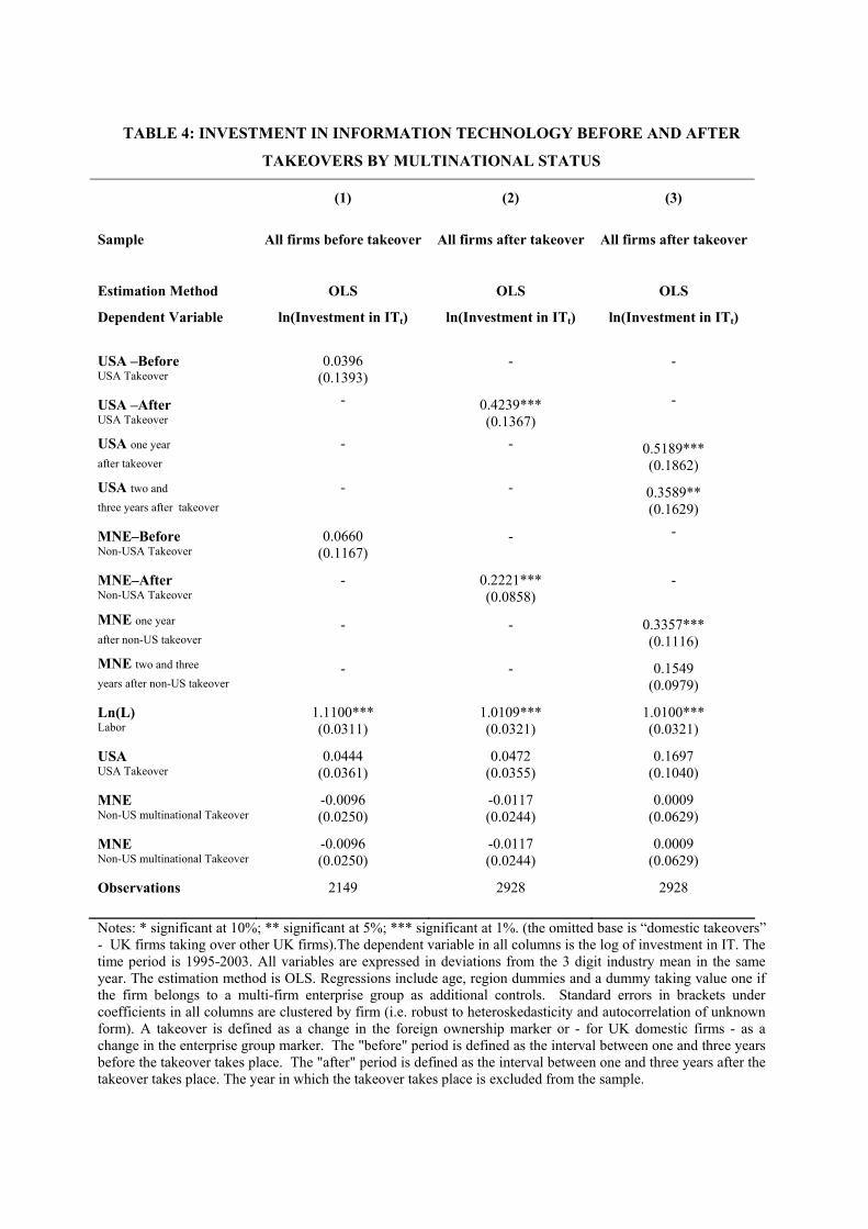
TABLE 4: INVESTMENT IN INFORMATION TECHNOLOGY BEFORE AND AFTER

TAKEOVERS BY MULTINATIONAL STATUS

(1) (2) (3)

Sample All firms before takeover All firms after takeover All firms after takeover

Estimation Method OLS OLS OLS

Dependent Variable ln(Investment in ITt) ln(Investment in ITt) ln(Investment in ITt) USA –Before 0.0396 - - USA Takeover (0.1393)

USA –After - 0.4239*** - USA Takeover (0.1367) USA one year - - 0.5189*** after takeover (0.1862) USA two and - - 0.3589** three years after takeover (0.1629)

MNE–Before 0.0660 - - Non-USA Takeover (0.1167)

MNE–After - 0.2221*** - Non-USA Takeover (0.0858) MNE one year - - 0.3357*** after non-US takeover (0.1116) MNE two and three - - 0.1549 years after non-US takeover (0.0979)

Ln(L) 1.1100*** 1.0109*** 1.0100*** Labor (0.0311) (0.0321) (0.0321)

USA 0.0444 0.0472 0.1697 USA Takeover (0.0361) (0.0355) (0.1040)

MNE -0.0096 -0.0117 0.0009 Non-US multinational Takeover (0.0250) (0.0244) (0.0629)

MNE -0.0096 -0.0117 0.0009 Non-US multinational Takeover (0.0250) (0.0244) (0.0629)

Observations 2149 2928 2928 Notes: * significant at 10%; ** significant at 5%; *** significant at 1%. (the omitted base is “domestic takeovers” - UK firms taking over other UK firms).The dependent variable in all columns is the log of investment in IT. The time period is 1995-2003. All variables are expressed in deviations from the 3 digit industry mean in the same year. The estimation method is OLS. Regressions include age, region dummies and a dummy taking value one if the firm belongs to a multi-firm enterprise group as additional controls. Standard errors in brackets under coefficients in all columns are clustered by firm (i.e. robust to heteroskedasticity and autocorrelation of unknown form). A takeover is defined as a change in the foreign ownership marker or - for UK domestic firms - as a change in the enterprise group marker. The "before" period is defined as the interval between one and three years before the takeover takes place. The "after" period is defined as the interval between one and three years after the takeover takes place. The year in which the takeover takes place is excluded from the sample.

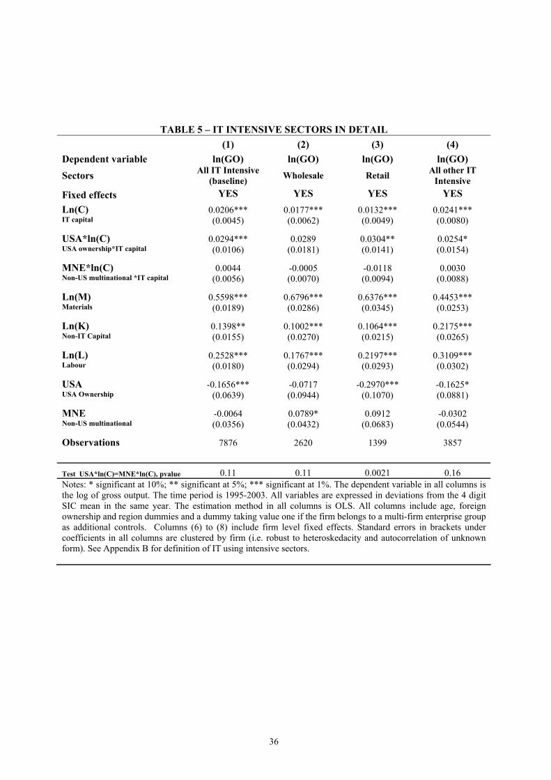
36

TABLE 5 – IT INTENSIVE SECTORS IN DETAIL (1) (2) (3) (4) Dependent variable ln(GO) ln(GO) ln(GO) ln(GO) Sectors All IT Intensive

(baseline) Wholesale Retail All other IT Intensive

Fixed effects YES YES YES YES Ln(C) 0.0206*** 0.0177*** 0.0132*** 0.0241*** IT capital (0.0045) (0.0062) (0.0049) (0.0080)

USA*ln(C) 0.0294*** 0.0289 0.0304** 0.0254* USA ownership*IT capital (0.0106) (0.0181) (0.0141) (0.0154)

MNE*ln(C) 0.0044 -0.0005 -0.0118 0.0030 Non-US multinational *IT capital (0.0056) (0.0070) (0.0094) (0.0088)

Ln(M) 0.5598*** 0.6796*** 0.6376*** 0.4453*** Materials (0.0189) (0.0286) (0.0345) (0.0253)

Ln(K) 0.1398** 0.1002*** 0.1064*** 0.2175*** Non-IT Capital (0.0155) (0.0270) (0.0215) (0.0265)

Ln(L) 0.2528*** 0.1767*** 0.2197*** 0.3109*** Labour (0.0180) (0.0294) (0.0293) (0.0302)

USA -0.1656*** -0.0717 -0.2970*** -0.1625* USA Ownership (0.0639) (0.0944) (0.1070) (0.0881)

MNE -0.0064 0.0789* 0.0912 -0.0302 Non-US multinational (0.0356) (0.0432) (0.0683) (0.0544)

Observations 7876 2620 1399 3857

Test USA*ln(C)=MNE*ln(C), pvalue 0.11 0.11 0.0021 0.16 Notes: * significant at 10%; ** significant at 5%; *** significant at 1%. The dependent variable in all columns is the log of gross output. The time period is 1995-2003. All variables are expressed in deviations from the 4 digit SIC mean in the same year. The estimation method in all columns is OLS. All columns include age, foreign ownership and region dummies and a dummy taking value one if the firm belongs to a multi-firm enterprise group as additional controls. Columns (6) to (8) include firm level fixed effects. Standard errors in brackets under coefficients in all columns are clustered by firm (i.e. robust to heteroskedacity and autocorrelation of unknown form). See Appendix B for definition of IT using intensive sectors.

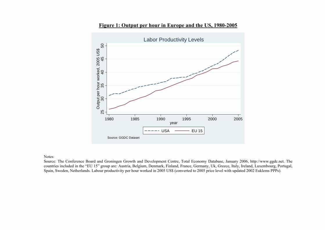
Figure 1: Output per hour in Europe and the US, 1980-2005

2530

3540

4550

Out

put p

er h

our w

orke

d, 2

005

US

$

1980 1985 1990 1995 2000 2005year

USA EU 15

Source: GGDC Dataset

Labor Productivity Levels

Notes: Source: The Conference Board and Groningen Growth and Development Centre, Total Economy Database, January 2006, http://www.ggdc.net. The countries included in the “EU 15” group are: Austria, Belgium, Denmark, Finland, France, Germany, Uk, Greece, Italy, Ireland, Luxembourg, Portugal, Spain, Sweden, Netherlands. Labour productivity per hour worked in 2005 US$ (converted to 2005 price level with updated 2002 Euklems PPPs).

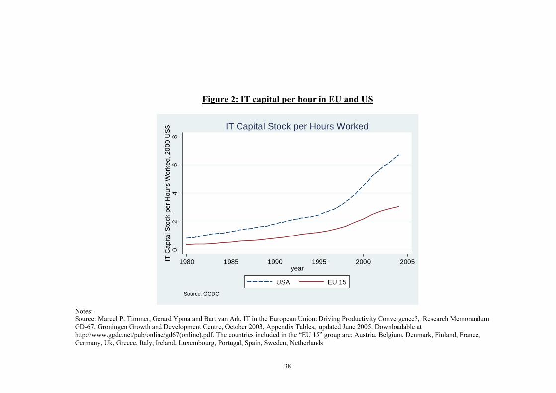
38

Figure 2: IT capital per hour in EU and US

02

46

8IT

Cap

ital S

tock

per

Hou

rs W

orke

d, 2

000

US

$

1980 1985 1990 1995 2000 2005year

USA EU 15

Source: GGDC

IT Capital Stock per Hours Worked

Notes: Source: Marcel P. Timmer, Gerard Ypma and Bart van Ark, IT in the European Union: Driving Productivity Convergence?, Research Memorandum GD-67, Groningen Growth and Development Centre, October 2003, Appendix Tables, updated June 2005. Downloadable at http://www.ggdc.net/pub/online/gd67(online).pdf. The countries included in the “EU 15” group are: Austria, Belgium, Denmark, Finland, France, Germany, Uk, Greece, Italy, Ireland, Luxembourg, Portugal, Spain, Sweden, Netherlands

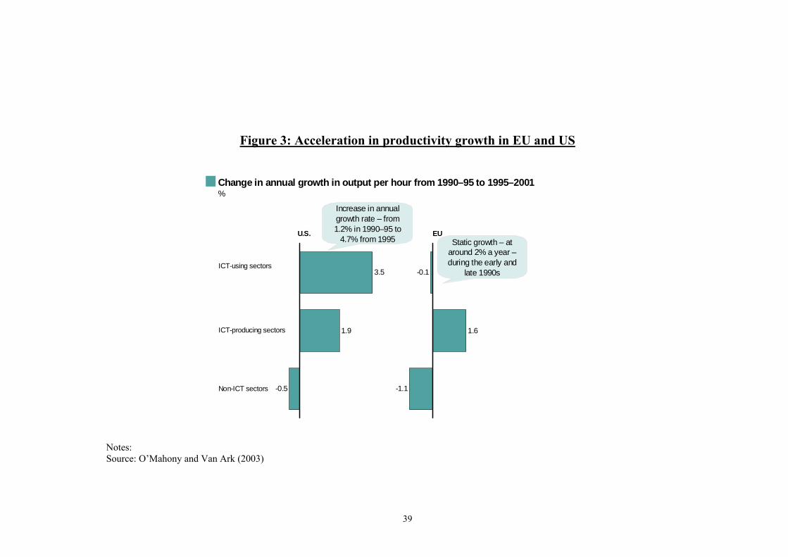
39

Figure 3: Acceleration in productivity growth in EU and US

Notes: Source: O’Mahony and Van Ark (2003)

Change in annual growth in output per hour from 1990–95 to 1995–2001%

3.5

1.9

-0.5

ICT-using sectors

ICT-producing sectors

Non-ICT sectors

U.S.

-0.1

1.6

-1.1

EU

Increase in annual growth rate – from 1.2% in 1990–95 to

4.7% from 1995 Static growth – at around 2% a year –during the early and

late 1990s

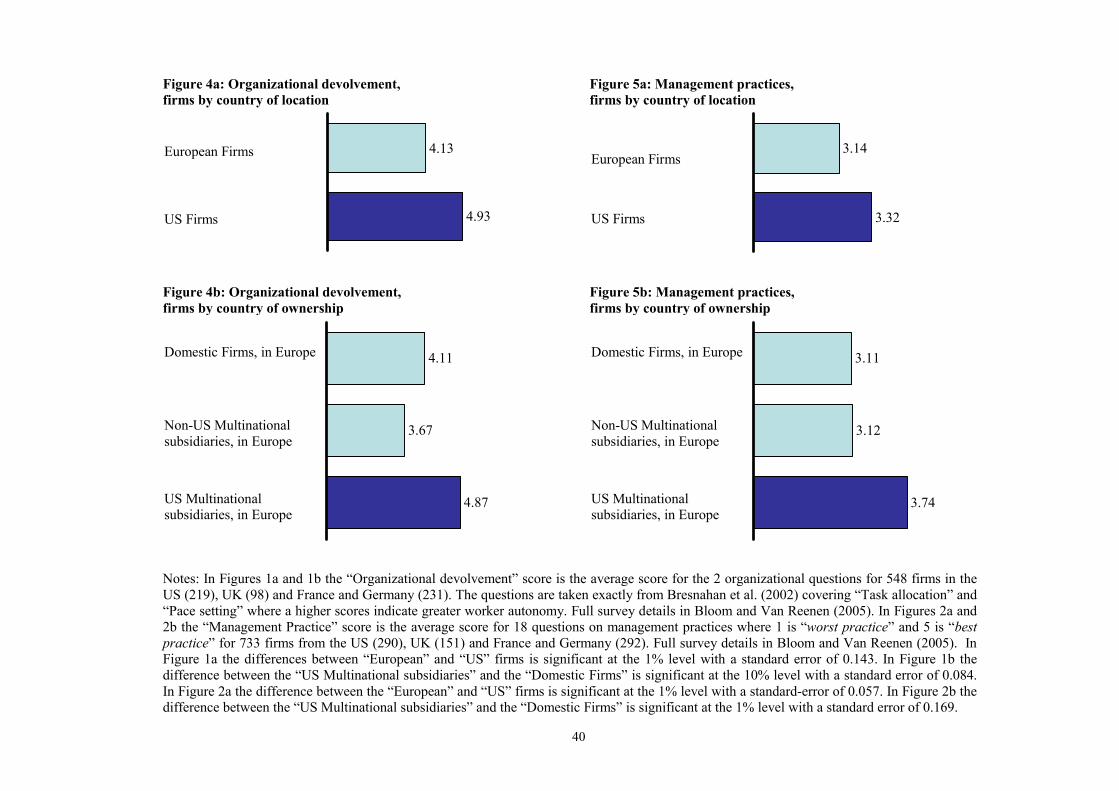
40

European Firms

3.74

3.12

3.11

Notes: In Figures 1a and 1b the “Organizational devolvement” score is the average score for the 2 organizational questions for 548 firms in the US (219), UK (98) and France and Germany (231). The questions are taken exactly from Bresnahan et al. (2002) covering “Task allocation” and “Pace setting” where a higher scores indicate greater worker autonomy. Full survey details in Bloom and Van Reenen (2005). In Figures 2a and 2b the “Management Practice” score is the average score for 18 questions on management practices where 1 is “worst practice” and 5 is “best practice” for 733 firms from the US (290), UK (151) and France and Germany (292). Full survey details in Bloom and Van Reenen (2005). In Figure 1a the differences between “European” and “US” firms is significant at the 1% level with a standard error of 0.143. In Figure 1b the difference between the “US Multinational subsidiaries” and the “Domestic Firms” is significant at the 10% level with a standard error of 0.084. In Figure 2a the difference between the “European” and “US” firms is significant at the 1% level with a standard-error of 0.057. In Figure 2b the difference between the “US Multinational subsidiaries” and the “Domestic Firms” is significant at the 1% level with a standard error of 0.169.

Domestic Firms, in Europe

Figure 4a: Organizational devolvement, firms by country of location

Figure 5a: Management practices, firms by country of location

3.32

3.14European Firms

4.13

4.93US Firms

Domestic Firms, in Europe

Non-US Multinational subsidiaries, in Europe

US Multinational subsidiaries, in Europe

Figure 4b: Organizational devolvement, firms by country of ownership

US Firms

Figure 5b: Management practices, firms by country of ownership

Non-US Multinational subsidiaries, in Europe

US Multinational subsidiaries, in Europe

4.87

3.67

4.11

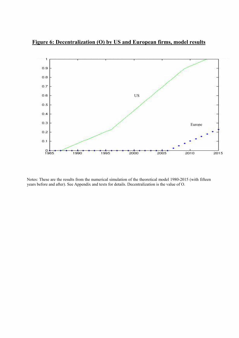
Figure 6: Decentralization (O) by US and European firms, model results

Notes: These are the results from the numerical simulation of the theoretical model 1980-2015 (with fifteen years before and after). See Appendix and texts for details. Decentralization is the value of O.

US

Europe

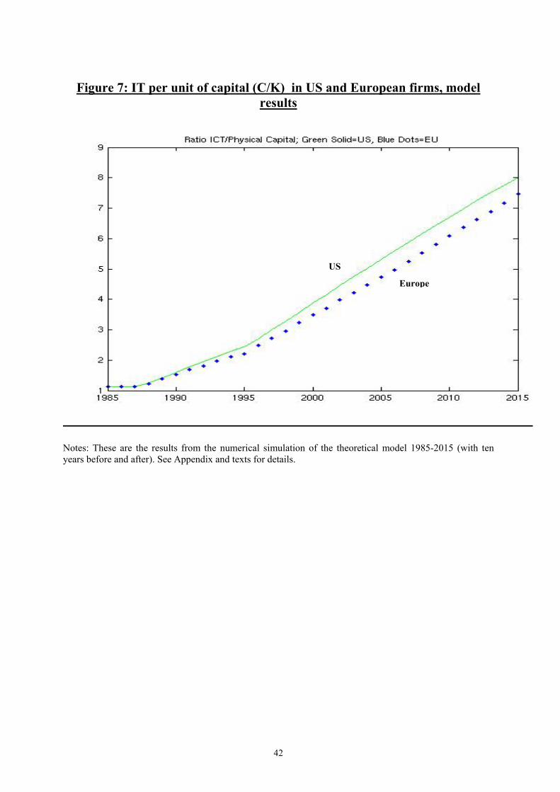
42

Figure 7: IT per unit of capital (C/K) in US and European firms, model results

Notes: These are the results from the numerical simulation of the theoretical model 1985-2015 (with ten years before and after). See Appendix and texts for details.

US

Europe

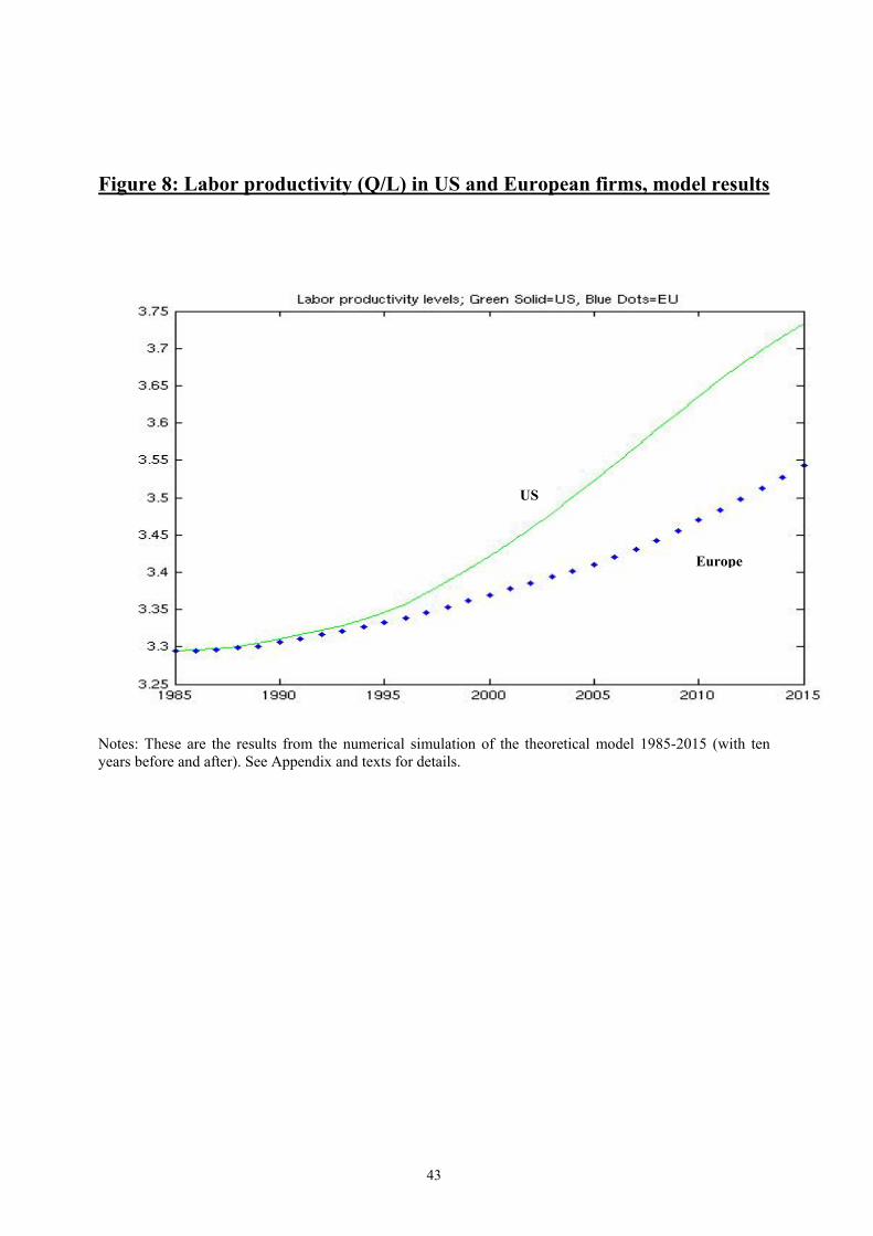
43

Figure 8: Labor productivity (Q/L) in US and European firms, model results

Notes: These are the results from the numerical simulation of the theoretical model 1985-2015 (with ten years before and after). See Appendix and texts for details.

US

Europe

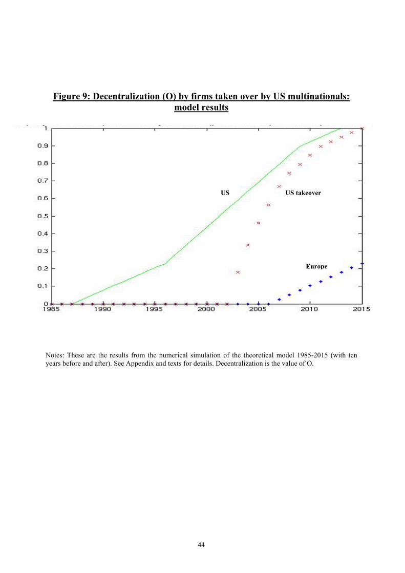
44

Figure 9: Decentralization (O) by firms taken over by US multinationals: model results

Notes: These are the results from the numerical simulation of the theoretical model 1985-2015 (with ten years before and after). See Appendix and texts for details. Decentralization is the value of O.

US US takeover

Europe

45

APPENDIX A: DATA AND ADDITIONAL RESULTS

A1 ESTABLISHMENT DATASET ABI The Annual Business Inquiry (ABI) is the major source of establishment level data in the UK. It underlies the construction of aggregate output and investment in the national accounts and is conducted by the Office of National Statistics (ONS) the UK equivalent of the US Census Bureau. The ABI is a stratified random sample: sampling probabilities are higher for large establishments (e.g. 100% for all establishments with more than 250 employees). Each establishment has a unique “reporting unit reference number” (RUREF) which does not change when a plant is taken over by a new firm. Data on the production sector (including manufacturing) is in the ABI which has a long time series element (from 1980 and before in some cases). Data on the non-production sector (services) is available for a much shorter time period (from 1997 onwards). The sample is large: in 1998 there are 28,765 plants in the production sector alone. The questionnaire sent out on the ABI is extensive and covers all the variables needed to estimate basic production functions. In particular it includes have gross output, value added, employment, wage bill, investment and total materials (this includes all intermediate inputs – energy, materials, etc.). The response rates to the ABI are high because it is illegal not to return the forms to the Office of National Statistics. A2 INFORMATION TECHNOLOGY DATASETS Overview Working closely with statisticians and data collectors at ONS we combined the four major IT surveys and matched this into the ABI establishment data using the common establishment code (the Inter-Departmental Business Register, or IDBR). The three IT hardware surveys were not designed to cover exactly the same establishments as contained in the ABI survey, but because there is over-sampling of the larger establishments in all surveys the overlap is substantial, especially for the larger plants. The main IT surveys include the Business Survey into Capitalized Items (BSCI), the Quarterly Inquiry into Capital Expenditure (QICE) and the Fixed Asset Register (FAR). The ABI also has additional questions on software included since 2000. These surveys are compiled at the reporting unit level, and contain information on the value (in thousands of pounds) of software and hardware acquisitions and disposals. Once the stocks are built within each different survey, we combine them across surveys and, for hardware and software separately, we build across-surveys stocks.28 We have some concerns about the accuracy of the plant reports of software expenditure (we are currently investigating these), so we focus in the main part of the paper on the IT hardware stocks. 28 We are careful to check for differences in coefficients due to the IT measures coming from different surveys. We could not reject the assumption that there were no significant differences in the IT coefficients arising from the fact that the IT stocks were built from different surveys.

46

In the following paragraphs we first describe the different surveys; we then illustrate the details of the Perpetual Inventory Method used for the construction of the capital stocks and the procedure followed to build across-surveys variables. Data Sources Business Survey into Capitalized Items (BSCI). The BSCI asks for detail of acquisitions and disposals of capital in more than 100 categories, including computer hardware and software. The survey is annual and runs between 1998 and 2003; we dropped the 1998 cross section due to concerns over reliability expressed by the data collectors. There is 100% sampling frame for the businesses with more than 750 employees and a stratified random sample of medium sized businesses (between 100 and 750 workers). The BSCI contributes about 1,500 to 2,000 observations for each year between 1999 and 2003. Quarterly Inquiry into Capital Expenditure (QICE). The QICE provides information on hardware and software investments from 2000Q1 until 2003Q4. The inquiry selects 32,000 establishments each quarter. Of these 32,000 companies, all establishments with over 300 employees are selected each quarter. Businesses with fewer employees are selected for the inquiry randomly. Each quarter one fifth of the random sample is rotated out of the sample and a new fifth is rotated in. The quarterly data have been annualized in several alternative ways and we checked the robustness of the results across these. First, we extrapolated within year for establishments with missing quarters29. As a second alternative, we constructed an indicator that gives the number of non-missing values that exist for each year and establishment and included this as an additional control in the regressions. Third, we dropped observations constructed from less than four full quarters. The results were quite robust across all three methods and the Tables report results based on the first method. Fixed Asset Register (FAR). The FAR asks for the historic cost (gross book value) of the fixed assets held on the firms’ asset register, broken down by the years of acquisition. The survey provides information on IT hardware assets only, and covers the years 1995 up to 2000. The survey provides information for about 1,000 hardware observations. Annual Business Inquiry (ABI). The ABI contains a question on software expenditures from 2000 onwards. There are approximately 20,000 non-zero returned values for software investments in each year. Estimation of IT capital stocks We build stocks of IT capital applying the Perpetual Inventory Method (PIM) to the IT investment data (and the non-IT investment data) described above. The basic PIM equation is:

( ) hit

hhit

hit KIK 11 −−+= δ (B1)

where h

tI represents real investment of asset type h (e.g. computer hardware, CtI ) and h

tδ is the asset specific depreciation rate. To construct real investment we deflate nominal investments using the economy-wide (asset specific) hedonic price indices for software and hardware

29 The extrapolation was done by simple averaging, but we also tried more sophisticated quarterly models taking into account the quarter surveyed. This made practically no difference.

47

provided by the NIESR (which are based on Jorgensen’s US price deflators). We rebased to the year 2000 for consistency with the other PPI deflators (see below). Estimation of TFP and capital services To calculate the user cost (e.g. ρC is the rental price of IT capital) we use the Hall-Jorgensen formulation:

ht

ht

ht

ht

htth

t

th

ht ppppr

TA )]/)(([

11

11 −−−−+−−

= δρ (B2)

where ρh is the rental price of asset class h, r is the nominal interest rate, δ is the depreciation rate of the asset, and p h is the asset price. The tax parameters are given by A which is the present-discounted value of depreciation allowances, and T which is the rate of corporate profits tax. We obtained user costs from the data underlying Oulton and Srinivasan (2004) kindly provided by the authors. These are economy wide We can then calculate total profits as30

ithh

th

it Kρ∑=Π (B3)

The share of each asset class in revenue is then

itt

it

it

ithh

tit

hht

h

ithh

th

ithh

thit Yp

KpY

K

KK

sΠ

Π==

∑∑

ρρ

ρρ

(B4)

that is used in calculating measured TFP in equation (7) and elsewhere. Zeros Both the BSCI and the QICE code missing values as zeros. While in the BSCI we are able to identify actual zero investments through a specific coding, for the QICE this is not possible. In the construction of the capital stocks we treated the zero investments observations as actual absence of IT investments. In the regressions we drop observations with zero IT capital stocks Interpolations In order to maximize the number of observations over which we could apply the PIM, we interpolated net investment observations for a single year of data if we observed investment the year before and the year afterwards. This affected only 2.8% of the observations in the regression sample and results are robust to dropping these observations. Initial Conditions

30 Note that empirically there are alternative ways to approach equation (B3). Our preferred method is to calculate

itt

it

it

ithh

thit Qp

Ks

ΠΠ

=ˆρ

where itΠ is taken from equation (B3) and itΠ is taken as the residual of revenues less

materials and the wage bill.

48

In order to apply the PIM methodology, we need to approximate a starting value to start the recursion. We apply a similar methodology as the one devised by Martin (2005) to construct establishment level capital stocks in the ARD. For each firm, we first build two digit industry-specific IT Investment/Capital ratios using the NISEC02 industry level data-set provided by the NIESR, which contains separate time-series data on hardware and software capital stocks and runs up to 2001 (these are based on the input-output tables starting in 1975). We then use the ratio of the establishment’s IT investment flow to the industry investment flow (denoted

Aitw for method “A”) to impute the IT capital stock (i.e. we are assuming that the

establishment’s share of the IT capital stock in the industry is equal to the establishment’s share of IT investment in the industry in the initial year). More precisely, we assume that for t = 0 only the initial plant level IT capital stock A

iC 0 is:

w; C w Ait

Ait0 ⎟

⎟⎠

⎞⎜⎜⎝

⎛=∈∀= C

jt

Cit

jtA

i II

jiC

where j represents an industry so a j sub-script represents an industry total – i.e. CjtI is total

industry IT investment and jtC is the total IT capital stock in time t. We apply this approximation to determine our initial condition in the first year that the establishment appears in our sample. For greenfield sites this is not an issue as their capital stock is zero. After the first year, we simply apply the PIM method. Some of the establishments that we observe only for the first time may be investing systematically at a different rate from the industry average. To check whether our results were driven by the methodology used to build the initial conditions, we considered an alternative methodology based on employment weights (method “B”). For the first time we observed a plant in our sample we assumed that:

( )

1

1

11

110

jiLL

w

ICwC

j

itBit

Citjt

Bit

Bi

∈∀=

+−=

−

−−

−− δ

So this is assuming that the establishment’s share of the industry IT stock in the initial period is equal to the establishment’s share of employment. Results are presented in Table A5 below and are consistent with the baseline method. Depreciation For all IT capital (software and hardware) we chose a depreciation rate of 36%. This choice is consistent with the analysis by methodology followed by the BEA which, in turn, derives from the study by Doms, Dunn, Oliner and Sichel (2004). In this study, the depreciation rate for PC’s is estimated at approximately 50%, this value including both obsolescence and reevaluation effects. Since – as the BEA - we use real IT investments we have to use a lower depreciation rate to avoid double counting of the revaluation effect, included in the price deflators. Basu et al (2003) argue that the true geometric rate of depreciation should be, in fact, approximately 30%. The significance and the magnitude of the coefficient obtained for both hardware and software are not affected by the exact choice of the alternative depreciation rate.

49

We also experimented with the extreme assumption of 100% depreciation rate for IT, thus working directly with the flows. Results are in Table A5 which shows a significant coefficient with a lower point estimate than in the main table (discussed below). Across-Survey Stocks Following the steps described above, we obtain hardware and software stocks within each different survey. We then matched our IT dataset with the ABI sample with non missing observations on other inputs and outputs (value added and gross output). In order to simplify the empirical analysis, we combined all the information of the different the surveys constructing overall across-surveys IT stocks for both hardware and software. Our strategy is to use the BSCI measure as the most reliable observation (as recommended by the data collectors). We then build our synthetic measure using the QICE stocks if the BSCI observation is missing or equal to zero and the QICE is different from zero. We finally use the FAR if both QICE and BSCI are missing and/or equal to zero and the FAR is not. For the software capital stock we also use the ABI information, following the same order described above. The sources of the aggregate capital stocks are summarized in the following table:

Source Hardware Capital Software Capital BSCI 3,704 2,387 QICE 17,517 13,049 FAR 686 881 ABI - 43,735

In order to keep track of the possible measurement error introduced using this procedure, we introduce in all the IT regressions a dummy that identifies the provenience of the observation for both the hardware and the software stocks. These dummies and their interactions with the IT coefficients are not significantly different from zero. A small portion of the firms included in our dataset responded to more than one survey. We use some of this overlapping sample to get a better understanding of the measurement error in the data. By comparing the reports from the same establishments we calculate that there is much more measurement error for software than for hardware, which is why we currently focus on hardware. We did not find any evidence that the measurement error for hardware was different for US firms than other firms, however, which is reassuring. A3 OTHER DATA PPI deflators We deflate gross output using the PPI deflators 2000 based provided by the ONS. For the manufacturing sector, the deflators are usually available at the 4 SIC digits level (MM17 PPI deflators). Whenever this was not the case, we used a general deflator for the 2 digit industry

50

or a deflator relative to the overall manufacturing sector. For the service sector we used a set of experimental deflators generated by the ONS. These deflators refer to a limited number of 5 SIC digits industries. For all the other industries we use the general deflator for the overall service sector. Skills In our analysis we use industry and/or region and/or year specific skills measures built using the Labour Force Survey data set. Our preferred measure of skills is the proportion of people in the sample having as a highest qualification a degree or equivalent and/or a title defined as “higher education” by the standard LFS classifications (post GSE A levels), even though the results are not qualitatively different once we use only the proportion of people with a degree. We use LFS data from 1993 to 2003. First, we keep only observations referring to people between 24 and 64 years. We drop observations for which no information is available on education. The cells over which the proportion is computed are defined by two digit industry, one digit region and year (we also considered four and three digit industry and area-only definitions). For each index, we drop observations that are based on less than 50 observations. We use the number of observations of the LFS cells as weights for the skills regressions. We also constructed similar datasets, containing information on education as well as wages and hours worked. These indexes are built only for observations having non-missing values for these additional variables. Alternative IT measure from the E-Commerce Survey The E-Commerce Survey was conducted in 2001, 2002 and 2003 with around 2,500 establishments in each cross section. Unfortunately these were random cross-sections so the overlap between years is minimal (preventing us from performing serious panel data analysis) Plant managers were directly asked “What proportion of your employees use a computer, workstation or terminal”. To construct an estimate of the number of employees using IT we multiplied this proportion by the number of workers in the establishment. Although this is conceptually much cruder than the IT capital stock, it has the advantage that we do not have to rely so much on assumptions concerning the initial conditions. In Table 2 we discuss the results from this measure, showing very similar results to those obtained from using the IT capital measure. A4 CLEANING We used standard procedures to clean the ABI and the IT data. First, we dropped all observations with negative value added and/or capital stock. Secondly we dropped the top and

bottom percentile of the distribution of XX∆ for employment and gross value added. Thirdly,

we dropped extreme values of total capital stock per employee and gross value added per employee. This step of the cleaning procedure was performed on the overall ARD sample. We applied a similar cleaning procedure also to our across surveys IT variables. For hardware IT variables (investments and capital stocks) we dropped the top and bottom percentiles of the ratio of the variables on gross value added31.

31 The results of the regression are qualitatively similar if the IT data are cleaned using the ratio of investments per employee or stocks per employee.

51

A5 DEFINITION OF I.T. INTENSIVE USING INDUSTRIES We focus on “IT intensive” sectors that are defined to be those that use IT intensively according to (Van Ark et al, 2002) who base their definitions on Stiroh (2002). The basic splits between industries that are intensive in “IT use” are based on the proportion of IT capital services in total capital services. This uses US data to calculate the service flows as these are more accurate than service flow calculations based on UK data. The industries are split based on the median proportion of IT capital service flows in total capital service flows. The IT intensive using sectors are listed in Table A1. Note that the other “non-IT intensive” sectors include the sectors that produce IT intensively. We also considered these as a separate category but found in relation to their IT coefficients they were significantly different from the sectors that used IT intensively. All industries are based on ISIC Revision 3. A6. TAKEOVERS The identification of takeovers consists of three basic steps. First, for all the available years (1980-2003 for manufacturing and 1997-2003 for services) we combine all the raw ARD data relative to selected and non selected firms. We thus create a register file that allows us to keep track of the whole history of each firm, and exploit the uniqueness of the reporting unit reference number to correct for obvious reporting problems (i.e. firms that disappear in one year, and appear again after some time). Second, for each firm we keep track of changes in the foreign ownership information and the enterprise group reference number to identify foreign and domestic takeovers32. Third, to control for measurement error in the takeover identification, we drop from the sample firms that are subject to more than three takeovers during their whole history and firms that experience consecutive takeovers within a three year time period.

A7 ADDITIONAL ECONOMETRIC RESULTS

Table A4 gives some additional production function results comparing alternative econometric techniques. These alternative methods attempt to control for endogeneity of the regressors in the presence of correlated unobserved heterogeneity (the within group estimates in the main text treat the inputs as strictly exogenous). The econometric methods are System GMM (GMM-SYS) of Blundell and Bond (2000) and the Olley Pakes (1996) method. Column (1) of Table A4 presents the results without fixed effects, but all other columns control for fixed effects. Across all specifications, all the factor inputs, including IT capital are positive and significant. In column (1) the sum of the coefficients on the factor shares is 0.99, very close to constant returns to scale. Column (2) includes a full set of 11,000 establishment specific fixed effects. The coefficients all remain significant at conventional levels. The coefficient on IT capital falls from 0.04 to 0.03, the coefficient on materials falls from 0.54 to 0.47. By contrast the coefficient on non-IT capital increases from 0.12 to 0.16 and the 32 Foreign takeovers are observed if a firm experiences a change in the foreign ownership marker. Domestic takeovers are observed if a UK firm changes its enterprise reference number. See Griffith et al (2002) for more details on the methodology.

52

coefficient on labor rises from 0.29 to 0.32. Compared to many other results in the micro production function literature33 the results here are reasonably stable when including fixed effects34. To implement the GMM system estimates we need to condition on a sample where we have at least three continuous time series observations (the OLS estimates keep all observations, even if we only observe an establishment for a single period). Column (3) conditions on the same sub-sample that we will estimate our GMM results on and re-runs the within groups estimate of column (2). The estimates are stable even after throwing away about three quarters of the sample. Column (4) presents the equivalent specification using GMM-SYS. The absence of higher order serial correlation and the failure of the Hansen-Sargan test to reject are consistent with the hypothesis that the instruments are valid. The coefficients on materials and non-IT capital fall and the coefficients on labour and IT capital rise compared to column (3). Column (5) implements a general dynamic model including lags of all the independent variables and the dependent variable. We then impose the common factor (COMFAC) restrictions by minimum distance and present these restricted estimates in the final column (note that we cannot reject the COMFAC restrictions as indicated by the diagnostics at the base of column (6)). The coefficient on IT (and the other factors) remains positive and significant with a coefficient of about 0.04 (similar to OLS levels in fact). Finally, column (6) implements a version of the Olley Pakes method. Although all the variables are significant at conventional levels this produces the lowest coefficient on IT capital in Table A4: 0.02.

33 Griliches and Mairesse (1997), Olley and Pakes (1996) or Levinsohn and Petrin (2003) 34 The transformation of variables into deviations from the industry mean helps stability and it may be that there is much less measurement error in this mandatory establishment survey than the typical firm study using accounting data.

53

TABLE A1: BREAKDOWN OF INDUSTRIES We concentrate on sectors that had a higher than median ICT capital services proportion of total capital services. We denote these the “IT intensive using sectors” (Group 1) and choose an identical typology to those in Van Ark et al (2002) who follow Stiroh (2002). These can be sub-divided into manufacturing and services (we found similar results in both IT intensive manufacturing and IT intensive services). The other two broad sectors are IT producing sectors (Group 2) and non-IT intensive sectors (Group 3). (Group 1) Sectors that intensively use ICT (“IT intensive using sectors”) IT-using manufacturing 18 Wearing apparel, dressing and dying of fur 22 Printing and publishing 29 Machinery and equipment 31, excl. 313 Electrical machinery and apparatus, excluding insulated wire 33, excl. 331 Precision and optical instruments, excluding IT instruments 351 Building and repairing of ships and boats 353 Aircraft and spacecraft 352+359 Railroad equipment and transport equipment 36-37 miscellaneous manufacturing and recycling IT-using services 51 Wholesale trades 52 Retail trade 71 Renting of machinery and equipment 73 Research and development 741-743 Professional business services (Group 2) Sectors that intensively produce ICT IT-producing manufacturing 30 Office Machinery 313 Insulated wire 321 Electronic valves and tubes 322 Telecom equipment 323 radio and TV receivers 331 scientific instruments IT producing services 64 Communications 72 Computer services and related activity (Group 3) Non- IT Intensive Sectors) Non-IT intensive manufacturing 15-16 Food drink and tobacco

54

17 Textiles 19 Leather and footwear 20 wood 21pulp and paper 23 mineral oil refining, coke and nuclear 24 chemicals 25 rubber and plastics 26 non-metallic mineral products 27 basic metals 28 fabricated metal products 34 motor vehicles Non-IT Services 50 sale, maintenance and repair of motor vehicles 55 hotels and catering 60 Inland transport 61 Water transport 62 Air transport 63 Supporting transport services, travel agencies 70 Real estate 749 Other business activities n.e.c. Non-IT intensive other sectors 10-14 Mining and quarrying 50-41 Utilities 45 Construction Notes This is the same three way division underlying Figure 2. Not all industries are represented because the ABI does not cover the public sector and the financial sector. Due to the dominance of state provision we also drop all industries relating to health and education.

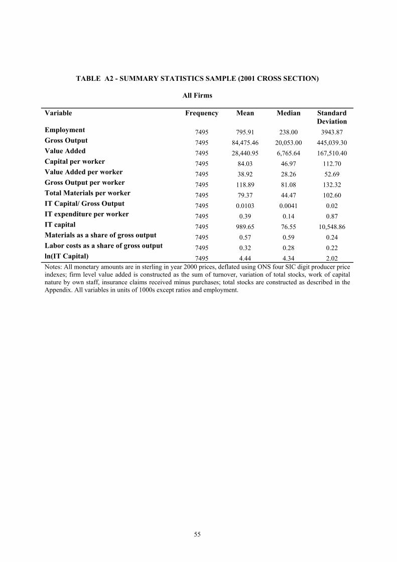
55

TABLE A2 - SUMMARY STATISTICS SAMPLE (2001 CROSS SECTION)

All Firms

Variable Frequency Mean Median Standard Deviation

Employment 7495 795.91 238.00 3943.87 Gross Output 7495 84,475.46 20,053.00 445,039.30 Value Added 7495 28,440.95 6,765.64 167,510.40 Capital per worker 7495 84.03 46.97 112.70 Value Added per worker 7495 38.92 28.26 52.69 Gross Output per worker 7495 118.89 81.08 132.32 Total Materials per worker 7495 79.37 44.47 102.60 IT Capital/ Gross Output 7495 0.0103 0.0041 0.02 IT expenditure per worker 7495 0.39 0.14 0.87 IT capital 7495 989.65 76.55 10,548.86 Materials as a share of gross output 7495 0.57 0.59 0.24 Labor costs as a share of gross output 7495 0.32 0.28 0.22 ln(IT Capital) 7495 4.44 4.34 2.02 Notes: All monetary amounts are in sterling in year 2000 prices, deflated using ONS four SIC digit producer price indexes; firm level value added is constructed as the sum of turnover, variation of total stocks, work of capital nature by own staff, insurance claims received minus purchases; total stocks are constructed as described in the Appendix. All variables in units of 1000s except ratios and employment.

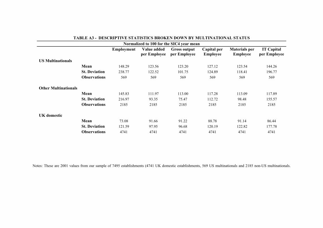
TABLE A3 - DESCRIPTIVE STATISTICS BROKEN DOWN BY MULTINATIONAL STATUS Normalized to 100 for the SIC4 year mean

Employment Value added per Employee

Gross output per Employee

Capital per Employee

Materials per Employee

IT Capital per Employee

US Multinationals Mean 148.29 123.56 123.20 127.12 123.54 144.26 St. Deviation 238.77 122.52 101.75 124.89 118.41 196.77 Observations 569 569 569 569 569 569 Other Multinationals Mean 145.83 111.97 113.00 117.28 113.09 117.89 St. Deviation 216.97 93.35 75.47 112.72 98.48 155.57 Observations 2185 2185 2185 2185 2185 2185 UK domestic Mean 73.08 91.66 91.22 88.78 91.14 86.44 St. Deviation 121.59 97.95 96.68 120.19 122.82 177.78 Observations 4741 4741 4741 4741 4741 4741

Notes: These are 2001 values from our sample of 7495 establishments (4741 UK domestic establishments, 569 US multinationals and 2185 non-US multinationals.

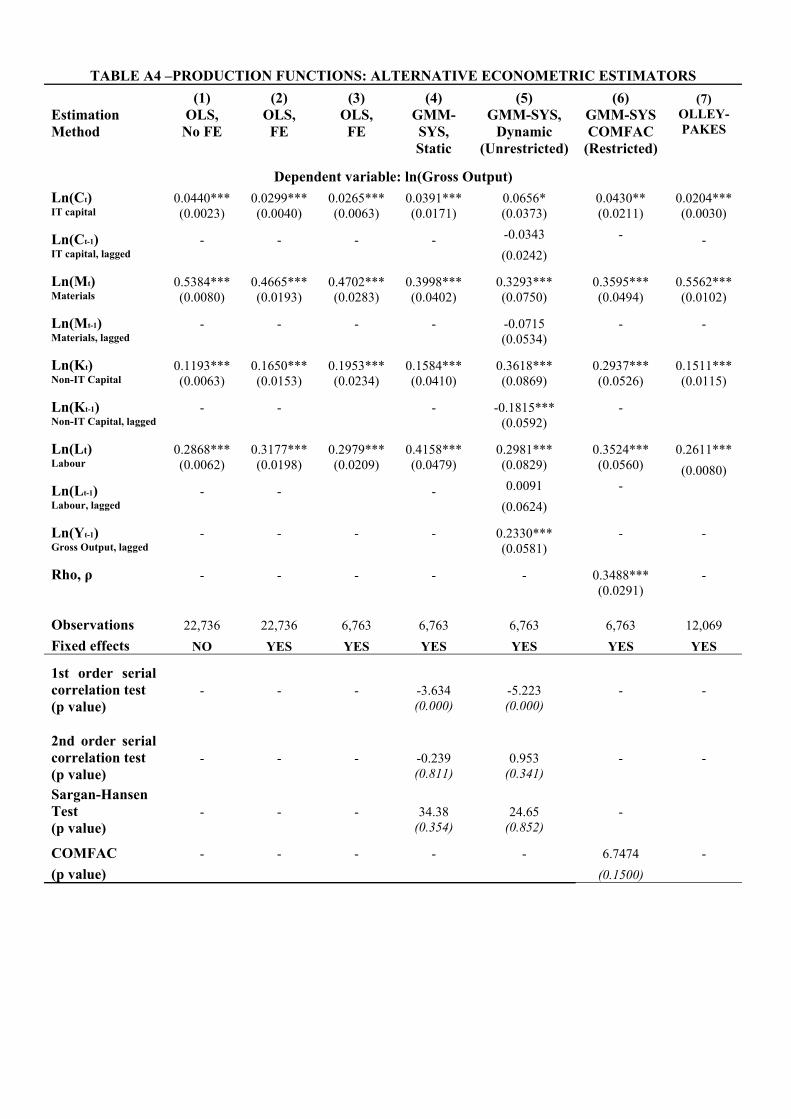
TABLE A4 –PRODUCTION FUNCTIONS: ALTERNATIVE ECONOMETRIC ESTIMATORS

(1) (2) (3) (4) (5) (6) (7) Estimation Method

OLS, No FE

OLS, FE

OLS, FE

GMM-SYS, Static

GMM-SYS, Dynamic

(Unrestricted)

GMM-SYS COMFAC

(Restricted)

OLLEY-PAKES

Dependent variable: ln(Gross Output) Ln(Ct) 0.0440*** 0.0299*** 0.0265*** 0.0391*** 0.0656* 0.0430** 0.0204*** IT capital (0.0023) (0.0040) (0.0063) (0.0171) (0.0373) (0.0211) (0.0030)

Ln(Ct-1) - - - - -0.0343 - - IT capital, lagged (0.0242)

Ln(Mt) 0.5384*** 0.4665*** 0.4702*** 0.3998*** 0.3293*** 0.3595*** 0.5562*** Materials (0.0080) (0.0193) (0.0283) (0.0402) (0.0750) (0.0494) (0.0102)

Ln(Mt-1) - - - - -0.0715 - - Materials, lagged (0.0534)

Ln(Kt) 0.1193*** 0.1650*** 0.1953*** 0.1584*** 0.3618*** 0.2937*** 0.1511*** Non-IT Capital (0.0063) (0.0153) (0.0234) (0.0410) (0.0869) (0.0526) (0.0115)

Ln(Kt-1) - - - -0.1815*** - Non-IT Capital, lagged (0.0592)

Ln(Lt) 0.2868*** 0.3177*** 0.2979*** 0.4158*** 0.2981*** 0.3524*** 0.2611*** Labour (0.0062) (0.0198) (0.0209) (0.0479) (0.0829) (0.0560) (0.0080) Ln(Lt-1) - - - 0.0091 - Labour, lagged (0.0624)

Ln(Yt-1) - - - - 0.2330*** - - Gross Output, lagged (0.0581)

Rho, ρ - - - - - 0.3488*** - (0.0291)

Observations 22,736 22,736 6,763 6,763 6,763 6,763 12,069 Fixed effects NO YES YES YES YES YES YES

1st order serial correlation test - - - -3.634 -5.223 - - (p value) (0.000) (0.000)

2nd order serial correlation test - - - -0.239 0.953 - - (p value) (0.811) (0.341) Sargan-Hansen Test - - - 34.38 24.65 - (p value) (0.354) (0.852)

COMFAC - - - - - 6.7474 - (p value) (0.1500)

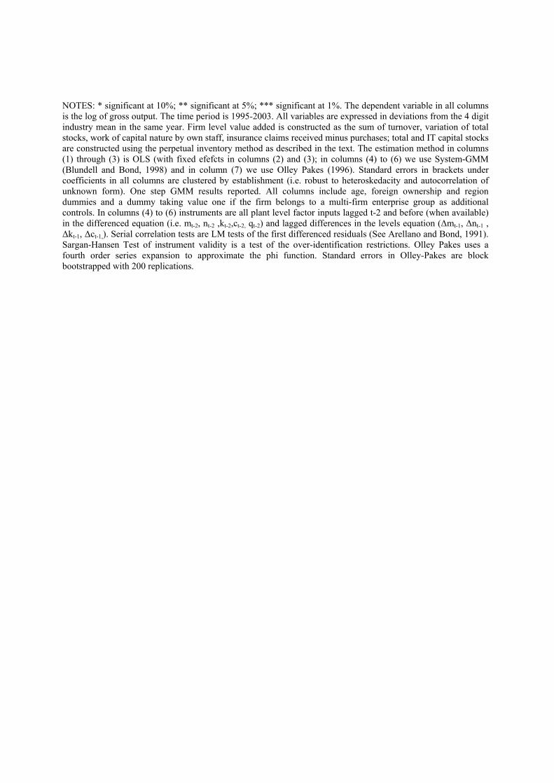
NOTES: * significant at 10%; ** significant at 5%; *** significant at 1%. The dependent variable in all columns is the log of gross output. The time period is 1995-2003. All variables are expressed in deviations from the 4 digit industry mean in the same year. Firm level value added is constructed as the sum of turnover, variation of total stocks, work of capital nature by own staff, insurance claims received minus purchases; total and IT capital stocks are constructed using the perpetual inventory method as described in the text. The estimation method in columns (1) through (3) is OLS (with fixed efefcts in columns (2) and (3); in columns (4) to (6) we use System-GMM (Blundell and Bond, 1998) and in column (7) we use Olley Pakes (1996). Standard errors in brackets under coefficients in all columns are clustered by establishment (i.e. robust to heteroskedacity and autocorrelation of unknown form). One step GMM results reported. All columns include age, foreign ownership and region dummies and a dummy taking value one if the firm belongs to a multi-firm enterprise group as additional controls. In columns (4) to (6) instruments are all plant level factor inputs lagged t-2 and before (when available) in the differenced equation (i.e. mt-2, nt-2 ,kt-2,ct-2, qt-2) and lagged differences in the levels equation (∆mt-1, ∆nt-1 , ∆kt-1, ∆ct-1,). Serial correlation tests are LM tests of the first differenced residuals (See Arellano and Bond, 1991). Sargan-Hansen Test of instrument validity is a test of the over-identification restrictions. Olley Pakes uses a fourth order series expansion to approximate the phi function. Standard errors in Olley-Pakes are block bootstrapped with 200 replications.

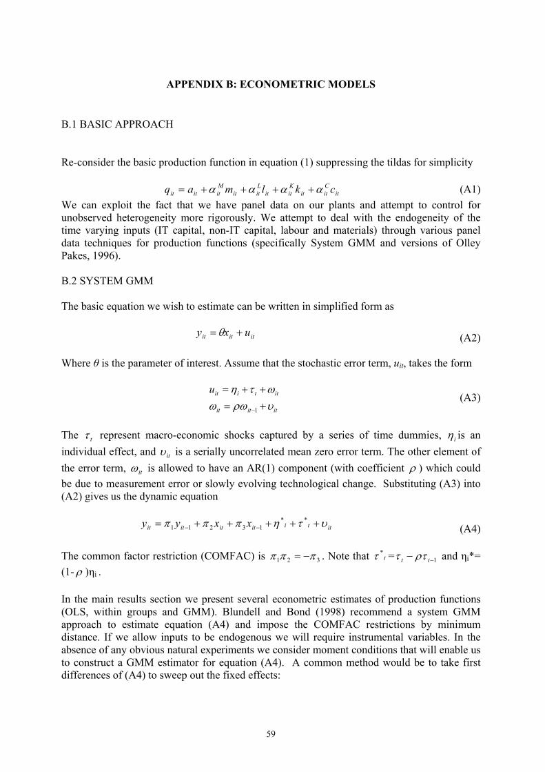
59

APPENDIX B: ECONOMETRIC MODELS B.1 BASIC APPROACH Re-consider the basic production function in equation (1) suppressing the tildas for simplicity

itCitit

Kitit

Litit

Mititit cklmaq αααα ++++= (A1)

We can exploit the fact that we have panel data on our plants and attempt to control for unobserved heterogeneity more rigorously. We attempt to deal with the endogeneity of the time varying inputs (IT capital, non-IT capital, labour and materials) through various panel data techniques for production functions (specifically System GMM and versions of Olley Pakes, 1996). B.2 SYSTEM GMM The basic equation we wish to estimate can be written in simplified form as

ititit uxy += θ (A2) Where θ is the parameter of interest. Assume that the stochastic error term, uit, takes the form

ititit

ittiituυρωωωτη

+=++=

−1

(A3)

The tτ represent macro-economic shocks captured by a series of time dummies, iη is an individual effect, and itυ is a serially uncorrelated mean zero error term. The other element of the error term, itω is allowed to have an AR(1) component (with coefficient ρ ) which could be due to measurement error or slowly evolving technological change. Substituting (A3) into (A2) gives us the dynamic equation

ittiitititit xxyy υτηπππ +++++= −−**

13211 (A4) The common factor restriction (COMFAC) is 321 πππ −= . Note that t

*τ = 1−− tt ρττ and ηi*= (1- ρ )ηi . In the main results section we present several econometric estimates of production functions (OLS, within groups and GMM). Blundell and Bond (1998) recommend a system GMM approach to estimate equation (A4) and impose the COMFAC restrictions by minimum distance. If we allow inputs to be endogenous we will require instrumental variables. In the absence of any obvious natural experiments we consider moment conditions that will enable us to construct a GMM estimator for equation (A4). A common method would be to take first differences of (A4) to sweep out the fixed effects:

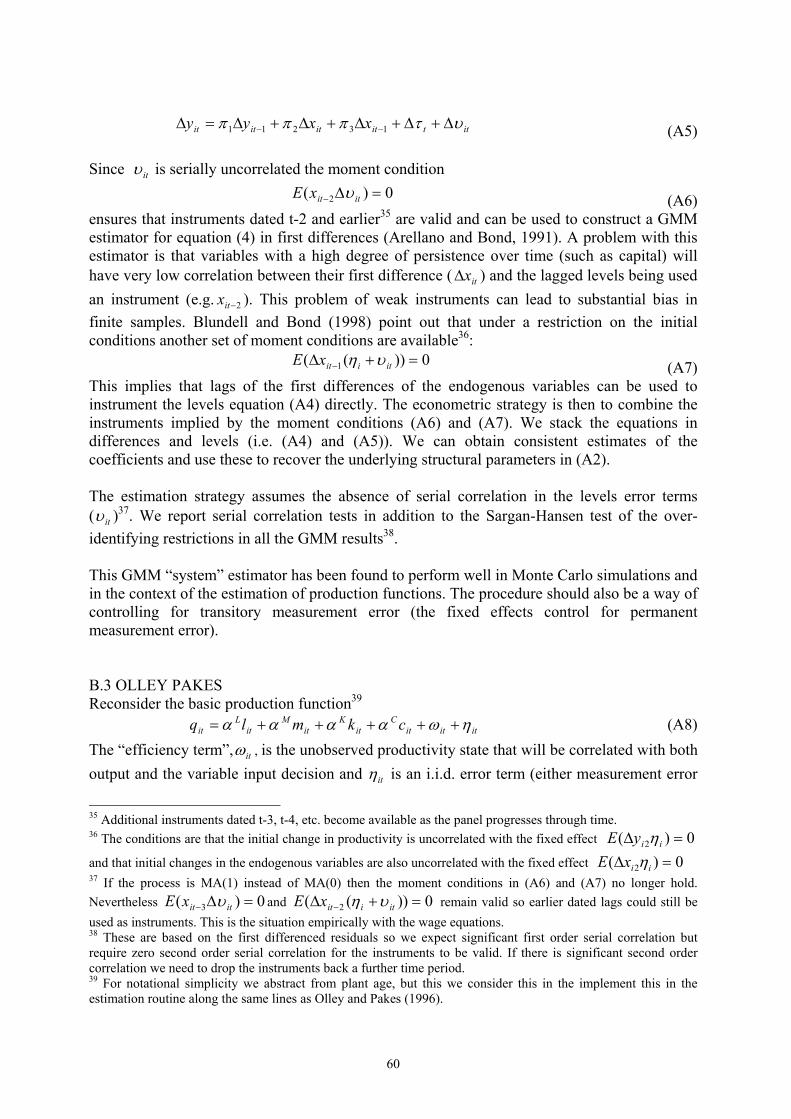
60

ittitititit xxyy υτπππ ∆+∆+∆+∆+∆=∆ −− 13211 (A5) Since itυ is serially uncorrelated the moment condition

0)( 2 =∆− ititxE υ (A6) ensures that instruments dated t-2 and earlier35 are valid and can be used to construct a GMM estimator for equation (4) in first differences (Arellano and Bond, 1991). A problem with this estimator is that variables with a high degree of persistence over time (such as capital) will have very low correlation between their first difference ( itx∆ ) and the lagged levels being used an instrument (e.g. 2−itx ). This problem of weak instruments can lead to substantial bias in finite samples. Blundell and Bond (1998) point out that under a restriction on the initial conditions another set of moment conditions are available36:

0))(( 1 =+∆ − itiitxE υη (A7) This implies that lags of the first differences of the endogenous variables can be used to instrument the levels equation (A4) directly. The econometric strategy is then to combine the instruments implied by the moment conditions (A6) and (A7). We stack the equations in differences and levels (i.e. (A4) and (A5)). We can obtain consistent estimates of the coefficients and use these to recover the underlying structural parameters in (A2). The estimation strategy assumes the absence of serial correlation in the levels error terms ( itυ )37. We report serial correlation tests in addition to the Sargan-Hansen test of the over-identifying restrictions in all the GMM results38. This GMM “system” estimator has been found to perform well in Monte Carlo simulations and in the context of the estimation of production functions. The procedure should also be a way of controlling for transitory measurement error (the fixed effects control for permanent measurement error). B.3 OLLEY PAKES Reconsider the basic production function39

itititC

itK

itM

itL

it ckmlq ηωαααα +++++= (A8) The “efficiency term”, itω , is the unobserved productivity state that will be correlated with both output and the variable input decision and itη is an i.i.d. error term (either measurement error

35 Additional instruments dated t-3, t-4, etc. become available as the panel progresses through time. 36 The conditions are that the initial change in productivity is uncorrelated with the fixed effect 0)( 2 =∆ iiyE η

and that initial changes in the endogenous variables are also uncorrelated with the fixed effect 0)( 2 =∆ iixE η 37 If the process is MA(1) instead of MA(0) then the moment conditions in (A6) and (A7) no longer hold. Nevertheless 0)( 3 =∆− ititxE υ and 0))(( 2 =+∆ − itiitxE υη remain valid so earlier dated lags could still be used as instruments. This is the situation empirically with the wage equations. 38 These are based on the first differenced residuals so we expect significant first order serial correlation but require zero second order serial correlation for the instruments to be valid. If there is significant second order correlation we need to drop the instruments back a further time period. 39 For notational simplicity we abstract from plant age, but this we consider this in the implement this in the estimation routine along the same lines as Olley and Pakes (1996).

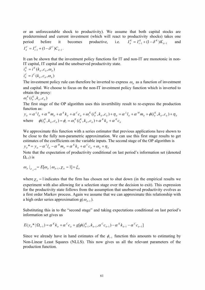
61

or an unforecastable shock to productivity). We assume that both capital stocks are predetermined and current investment (which will react to productivity shocks) takes one period before it becomes productive, i.e. 11 )1( −− −+= it

KKt

Kit KII δ and

11 )1( −− −+= itCC

tCit CII δ .

It can be shown that the investment policy functions for IT and non-IT are monotonic in non-IT capital, IT capital and the unobserved productivity state.

),,( itititKK

it ckii ω= ),,( ititit

CCit ckii ω=

The investment policy rule can therefore be inverted to express itω as a function of investment and capital. We choose to focus on the non-IT investment policy function which is inverted to obtain the proxy:

),,( ititKit

Kt ckiω

The first stage of the OP algorithm uses this invertibility result to re-express the production function as:

itititKitit

Mit

Lititit

Kit

Ktit

Cit

Kit

Mit

Lit ckimlckickmly ηφααηωαααα +++=+++++= ),,(),,(

where itK

itK

ititKit

Kttitit

Kit ckckicki ααωφφ ++== ),,(),,(

We approximate this function with a series estimator that previous applications have shown to be close to the fully non-parametric approximation. We can use this first stage results to get estimates of the coefficients on the variable inputs. The second stage of the OP algorithm is

itititC

itK

itM

itL

itit ckmlyy ηωαααα +++=−−=* Note that the expectation of productivity conditional on last period’s information set (denoted Ωt-1) is

ititititit Eit

ξχωωω χ +== −=]1,|[| 11

where 1=itχ indicates that the firm has chosen not to shut down (in the empirical results we experiment with also allowing for a selection stage over the decision to exit). This expression for the productivity state follows from the assumption that unobserved productivity evolves as a first order Markov process. Again we assume that we can approximate this relationship with a high order series approximation g( 1−itω ). Substituting this in to the “second stage” and taking expectations conditional on last period’s information set gives us

]),,([)|*( 111111 −−−−−− −−++=Ω itC

itK

itC

itKitit

Cit

Ktit ckckigckyE αααφαα

Since we already have in hand estimates of the 1−tφ function this amounts to estimating by Non-Linear Least Squares (NLLS). This now gives us all the relevant parameters of the production function.

62

There are numerous extensions to the basic Olley-Pakes methodology that have been suggested. One we considered was the additional selection correction originally suggested by the authors, but this made little difference to the results so the tables report the non-selectivity corrected results.