1

Downside market risk of carry trades

Victoria Dobrynskaya1

First version: March 2010

This version: March 2013

Abstract

Carry trades consistently generate high excess returns with high Sharpe ratios. I

propose a new factor - the downside market factor - to explain the high currency

returns. I show that carry trades crash systematically in the worst states of the

world, when the stock market plunges or a disaster happens. High-interest

currencies have significantly high downside market betas and significantly

negative coskewness with the stock market, while low-interest currencies can

serve as a hedging instrument against the downside market risk. The downside

market factor can explain the returns to currency portfolios, sorted by the forward

discount, better than other factors previously proposed in the literature. GMM

estimates of the downside beta premium are similar in the currency and stock

markets, statistically significant and close to its theoretical value. Therefore, the

high returns to carry trades are a fair compensation for their high downside market

risk.

JEL classification: G12, G15, F31

Keywords: carry trades, currency risk, downside risk, downside beta, coskewness,

crash risk

*London School of Economics, Houghton St. London WC2A 2AE, v.v.dobrynskaya@lse.ac.uk.

I am very grateful to Christian Julliard, Christopher Polk, Andrea Vedolin, Mungo Wilson, Sergei Guriev, Adien

Verdelhan, Craig Burnside, Philippe Mueller, Marcela Valenzuela and seminar participants at London School of

Economics, International College of Economics and Finance, New Economic School, London Business School,

Multinational Finance Society meeting and the Annual Congress of the European Economic Association for their

comments and suggestions. I thank Lucio Sarno for providing the data on their volatility factor. Colm O‟Sullivan

provided excellent research assistance.

This study was carried out within the National Research University Higher School of Economics‟ Academic Fund

Program in 2009-2010, research grant No.10-01-0069.

2

1. INTRODUCTION

One of the puzzles in international finance, which challenges the traditional theory, is the

forward premium puzzle, or the violation of the Uncovered Interest Parity (UIP). According to the

UIP, free capital mobility ensures that investments in different currencies with different levels of

local interest rates do not consistently generate excess returns, because a negative interest rate

differential should be compensated by the expected exchange rate appreciation of the target

currency, or the forward premium. In reality, though, this does not happen, but the opposite is

observed quite often: high-interest currencies tend to appreciate while low-interest currencies tend

to depreciate, on average (Fama, 1984). Then, investments in high-interest currencies consistently

generate higher expected returns than investments in low-interest currencies. This empirical

„anomaly‟ has led to the growing popularity of carry trades – an investment strategy where an

investor borrows in low-interest currencies and invests into high-interest currencies.

The aim of this paper is to answer the question: Are the high returns to carry trades a fair

compensation for their risk? Brunnermeier at al. (2008) show that high-interest currencies tend to

crash occasionally and their returns are negatively skewed2. But nonsystematic crashes should not

matter for a diversifying investor and, hence, cannot rationalize high returns. What should matter is

the systematic covariance of carry trade returns with the stochastic discount factor. There is an

ongoing debate whether carry trade portfolios have significant covariances (or betas) with the

stochastic discount factor and whether these covariances can explain the cross-section of currency

returns. Lustig and Verdelhan (2007) suggest that consumption CAPM can explain the returns to

carry trades because higher interest rate currencies have higher consumption betas. However,

Burnside (2011) argues that consumption betas of currency portfolios are statistically insignificant

and economically too small to rationalize high carry trade returns and concludes that consumption

risk explains none of the cross-sectional variation in the expected returns of currency portfolios.

Burnside (2012) studies whether traditional factor models, the CAPM, the Fama-French three factor

model and the CAPM with industrial production, can explain the returns to carry trades. He finds

that they cannot, because the returns to carry trade portfolios are either uncorrelated with the US

market factors, or the market betas are too small and the models estimated for currency and stock

portfolios jointly are rejected. He concludes that “there is no unifying risk based explanation of

returns in these two markets”.

In this paper I show that once we look at the downside market risk of currency portfolios,

everything falls into place. High interest rate currencies have significantly higher downside market

2 A number of papers quantify the crash risk of carry trades and estimate the crash risk premium (e.g. Fahri et al., 2009,

Jurek, 2009, Chernov et al., 2012).

3

risk, measured by downside beta or coskewness, while low interest rate currencies have zero

downside risk and, hence, can serve as a hedging instrument. Whereas consumption betas or market

betas of carry trade portfolios are small and sometimes insignificant, downside market betas are

several times higher and statistically significant, especially if we measure them in the worst states of

the world, e.g. when there is a market crash or a disaster event.

Downside risk is a better measure of risk because it shows the covariance of an asset‟s return

with the market in the worst states of the world when the overall market performs poorly and the

marginal utility of investors is high. If an asset performs poorly in such states, it is highly

unattractive and should provide high expected returns. Ang, Chen and Xing (2006) show that this is

the case in the stock market. They provide an asset pricing model with downside and upside betas

and show that the downside beta has higher explanatory power than the average beta while the

upside beta is not priced at all. In an alternative asset pricing model – the three-moment CAPM by

Harvey and Siddique (2000), assets with lower coskewness with the market should provide higher

expected returns because they perform poorly in states of high market volatility. The authors show

that adding coskewness to the asset pricing regressions improves their explanatory power in the

cross-section of stock returns. Coskewness can be considered as another measure of downside risk

because high market volatility is usually observed on the downside.

I show that the spread in the downside market betas and coskewness across interest-rate-

sorted currency portfolios is sufficient to justify the spread in their returns. The GMM estimates of

the downside beta and coskewness premiums in the currency market are highly significant.

Estimation of the downside beta or coskewness CAPM for currency and stock portfolios jointly

produces a good fit of the models, while the traditional CAPM is rejected on several grounds. The

spread in the traditional market betas across currency portfolios is insufficient, the estimate of the

market beta premium is too high compared to its theoretical value and the overall fit of the model is

worse in both currency and stock markets. The downside risk, measured by the downside beta or

coskewness, has much higher explanatory power for the cross-section of returns in the both

markets. The downside risk premiums are similar in the both markets and close to the theoretical

value of 1 percent per month. In fact, I cannot reject the hypothesis that the downside risk is priced

similarly in the currency and stock markets. I conclude that the high excess returns to carry trades

are not a free lunch but rather a fair compensation for their high downside market risk.

The results are robust to different levels of diversification within carry trade portfolios,

different estimation methods employed (GMM with identity and efficient weighting matrices and

Fama-MacBeth with time-varying betas), different cut-off levels for the downside betas, and

different samples of countries (the whole sample of developed and emerging economies, and a sub-

4

sample of developed countries). The downside market risk factor also wins the „horse race‟ between

alternative risk factors, previously proposed in the literature on carry trades. The results are even

stronger in the first decade of the 21st century – the period of rising popularity of carry trades among

institutional investors.

The co-movement of several major currencies with the stock market has already been

explored in Campbell et al. (2010) and Ronaldo and Söderlind (2010). Campbell et al. (2010) find a

positive correlation of the Australian dollar and the Canadian dollar with the global equity markets

and a negative correlation of the euro and the Swiss franc (the Japanese yen, the British pound and

the US dollar fall in the middle of the two extremes). A high-frequency analysis in Ronaldo and

Söderlind (2010) uncovers a similar pattern: the Swiss franc and the Japanese yen (and to a lesser

extent the euro) appreciate when the US stock market goes down, while the opposite is observed for

the British pound. The “safe haven” properties of the Swiss franc and the Japanese yen are

confirmed in periods of political, natural or financial disasters. Although these two studies do not

look at carry trades explicitly, their findings suggest that there is a particular relationship between

local interest rates and the hedging properties of the currencies. In both papers, the currencies which

go against the stock market are the ones which are the most common funding currencies for carry

trades (the Japanese yen and the Swiss franc), while the currencies with the highest exposure to the

stock market are the usual target currencies. Hence, carry trades may be prone to high stock market

risk, and this idea is explored thoroughly in my paper.

Instead of looking at single currencies, I form portfolios of currencies sorted by the forward

discount. This allows me to diversify away the idiosyncratic risk and to concentrate on those

properties which are attributable to currencies with different levels of interest rates. I include 42

developed and emerging economies in the sample, and hence I provide evidence for a much wider

spectrum of currencies than in the papers cited above. I show that there is a systematic positive

relationship between the market risk of a currency and the level of the local interest rate, and this

relationship is stronger for currencies of emerging markets. Moreover, this relationship is even

stronger if we measure the market risk on the downside. High-interest currencies tend to crash

together with the stock market while low-interest currencies are a „safe haven‟.

The rest of the paper is organized as follows. In section 2 I briefly review the related

empirical literature on currency returns and motivate the study of the downside risk by describing

theoretical asset pricing models with downside risk. Section 2.3 is devoted to the description of data

and currency portfolio formation. In section 3 I present the portfolio statistics and the main results

of estimation of alternative asset-pricing models by GMM. I also compare the downside risk pricing

in the currency and stock markets and run „horse races‟ between alternative risk factors. In section 4

5

I do a number of robustness tests. I consider different cut-off levels for the downside market beta

and disaster beta, I study alternative sets of currency portfolios, I look at the period of active carry

trades separately, and I use alternative estimation techniques. Section 5 concludes.

2. RELATED LITERATURE AND DATA

2.1. Empirical literature on currency returns

Several asset-pricing models have been proposed to explain the returns to carry trades. Lustig

and Verdelhan (2007) were the first who proposed sorting currencies by the level of nominal

interest rate into portfolios and study the cross-section of returns to these carry trade portfolios.

They look at carry trades through the consumption CAPM lenses and find that returns of high-

interest currencies co-move with US non-durable and durable consumption growth, while returns of

low-interest currencies serve as hedge against the domestic consumption risk. Hence, they

conclude, the high average returns of carry trades are a compensation for the consumption risk

because carry trades yield low returns when consumption growth is low and the marginal utility of

wealth is high. The relevance of the consumption CAPM framework for explaining currency returns

was also confirmed by De Santis and Fornari (2008) for several European countries.

Burnside (2011), in his comment on Lustig and Verdelhan‟s paper, argues that the

consumption risk explains none of the cross-sectional variation in carry trade returns. He finds that

while the consumption betas of carry trade portfolios increase with the level of interest rate, they are

all statistically not different from zero, and there is no statistically significant spread in these betas.

If the rank of betas is low, perhaps zero, there are problems with weak identification of the beta

premium. Moreover, the estimates of the consumption risk premium in the second pass regressions

in Lustig and Verdelhan (2007) do not account for the fact that the betas are generated regressors.

Burnside (2011) shows that the estimates of the consumption risk premium are statistically

insignificant once the standard errors are appropriately corrected (Shanken, 1992, or GMM). Also,

the consumption CAPM performs poorly (low R2) if the constant is restricted to zero. So, the

consumption CAPM is rejected on many grounds.

In their reply to Burnside, Lustig and Verdelhan (2011) provide additional evidence in favor

of the consumption CAPM. They show that their results are particularly visible during the global

financial crisis of 2008 when carry trades crashed, and the consumption growth was low. They

show that the OLS consumption beta of the HML3 currency portfolio is significant and that the

3HML here stands for “high-minus-low” currency portfolio which has a long position in high interest rate currencies

and a short position in low interest rate currencies. This term was brought to currency literature by Lustig, Roussanov

and Verdelhan (2011).

6

constant becomes small if they consider long-short carry trade portfolios, which are immune to the

dollar risk. By looking at data with higher frequency, they show that the consumption risk factor

loadings of carry returns vary over time and tend to increase during recessions and other crisis

episodes. Therefore, their estimates of consumption betas on quarterly data understate the true risk.

They also provide some evidence on the US stock market risk of carry trades and show that the

correlation with the stock market increases during financial crisis episodes. Overall, they conclude

that “the forward premium puzzle has a risk-based explanation”.

Burnside (2012) still does not believe this. He studies whether the CAPM, the Fama-French

three factor model, and models with industrial production and stock market volatility can explain

the returns to carry trades. He analyses only two carry trade portfolios: EW is an equally-weighted

portfolio of all currencies, and HML is a portfolio with a long position in high-interest currencies

and a short position in low-interest currencies. He finds that the US market betas of these two

portfolios are too small to rationalize their returns. He estimates the asset-pricing models using the

25 Fama-French stock portfolios and the two currency portfolios together, and finds that the pricing

errors for the currency portfolios are significant and the models are rejected. He concludes that the

traditional risk factors, which explain stock returns, cannot explain the returns to carry trades. A

discussion of his estimation methods is given in section 3.3 of this paper.

In the meanwhile, other risk factors have been proposed to explain the currency returns. These

risk factors are derived from currency portfolios themselves, sorted by some characteristics.

Examples are the HML carry factor (Lustig et al., 2011), global currency volatility factor

(Menkhoff et al., 2012a), global currency skewness factor (Rafferty, 2011), FX correlation risk

factor (Mueller et al., 2012), dollar factor (Verdelhan, 2012). Although these risk factors are

successful in explaining the carry trade returns, they fail to explain stock portfolio returns (e.g.

Burnside, 2012). Hence, Burnside argues, “there is no unifying risk-based explanation of returns in

these two markets”.

In this paper I provide ample evidence in favor of the market risk-based explanation of carry

trade returns. But rather than using the traditional market betas as a risk measure, I use downside

betas and coskewness, which condition on the market return being low or the market volatility

being high. These measures of downside risk concentrate on the worst states of the world when the

marginal utility of wealth is high and asset returns are particularly important. These measures of

downside risk proved to have higher explanatory power in the stock market (Ang, Chen and Xing,

2006, and Harvey and Siddique, 2000), and they explain the cross-section of returns of carry trade

portfolios better. In fact, I show that the downside risk is priced similarly in the currency and stock

markets. I also contribute to the debate between Lustig and Verdelhan (2007, 2011) and Burnside

7

(2011) about the explanatory power of the consumption CAPM in the currency market. I show that

the downside consumption risk of carry trades is much stronger, but still insufficient to explain the

cross-section of currency returns.

In a recent independent study, Lettau et al. (2013) also look at the downside risk CAPM in the

cross-section of currency, equity, bond and commodity portfolios. Our papers agree that the model

with the downside market factor has better explanatory power than the traditional CAPM. However,

our papers are different in several respects. First, we employ different methodologies (Lettau et al.

(2013) use Fama-MacBeth (1973) estimates, and I use GMM estimates, which take into account the

fact that betas are generated regressors). Second, in addition to the downside market beta, I consider

other measures of downside risk (downside consumption beta, coskewness, „extreme‟ downside

beta and „disaster‟ beta), and I show that the „extreme‟ downside risk measures have even higher

explanatory power for carry trades. Third, I compare the downside market factor to other currency

risk factors proposed in the literature and run „horse races‟. I also study a period of active carry

trades by institutional investors separately, and I show that all the results are stronger in this period,

thereby providing empirical support for the Basak and Pavlova (2012) model of the effects of

institutional trading.

2.2. Asset pricing models with downside risk

2.2.1. Three-moment CAPM with beta and coskewness

Since currency returns are distributed asymmetrically (Brunnermeier at al., 2008), we should

call for a model where the third moment is priced – the three-moment CAPM. The three-moment

CAPM goes back to Kraus and Litzenberger (1976), where there is preference for systematic

skewness. But for a diversifying investor, it is coskewness with the market which is important.

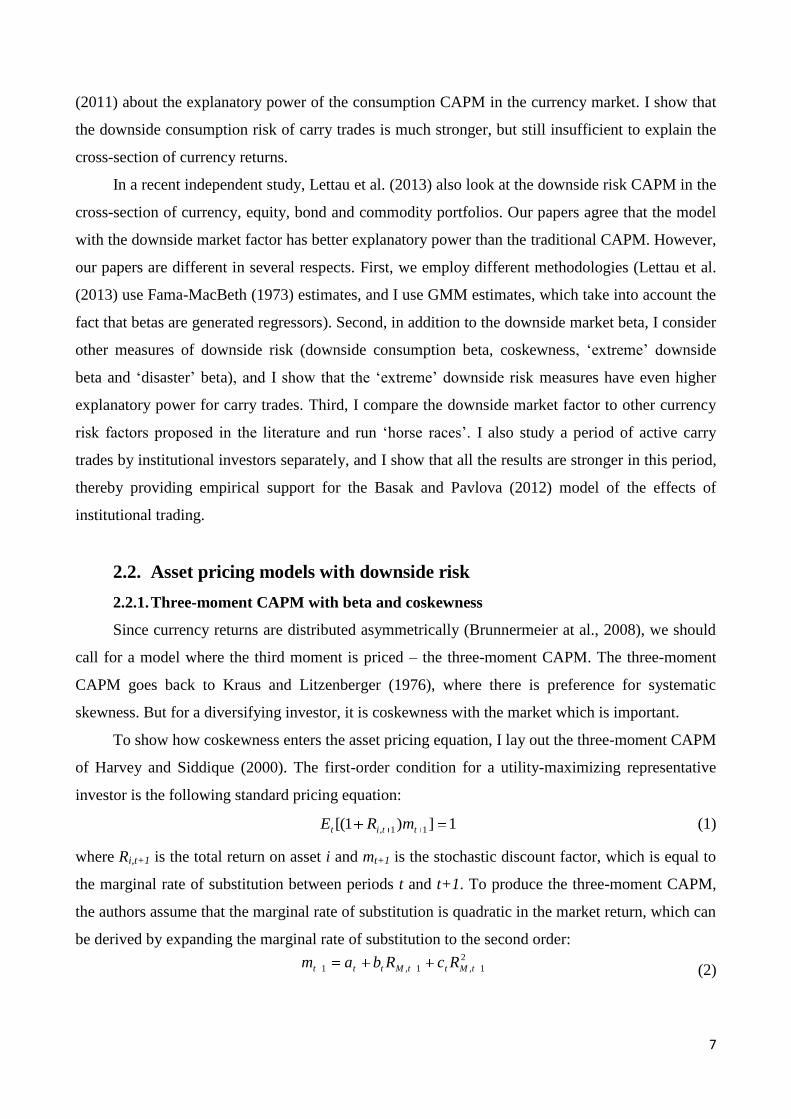
To show how coskewness enters the asset pricing equation, I lay out the three-moment CAPM

of Harvey and Siddique (2000). The first-order condition for a utility-maximizing representative

investor is the following standard pricing equation:

1])1[( 11, ttit mRE (1)

where Ri,t+1 is the total return on asset i and mt+1 is the stochastic discount factor, which is equal to

the marginal rate of substitution between periods t and t+1. To produce the three-moment CAPM,

the authors assume that the marginal rate of substitution is quadratic in the market return, which can

be derived by expanding the marginal rate of substitution to the second order: 2

1,1,1 tMttMttt RcRbam (2)

8

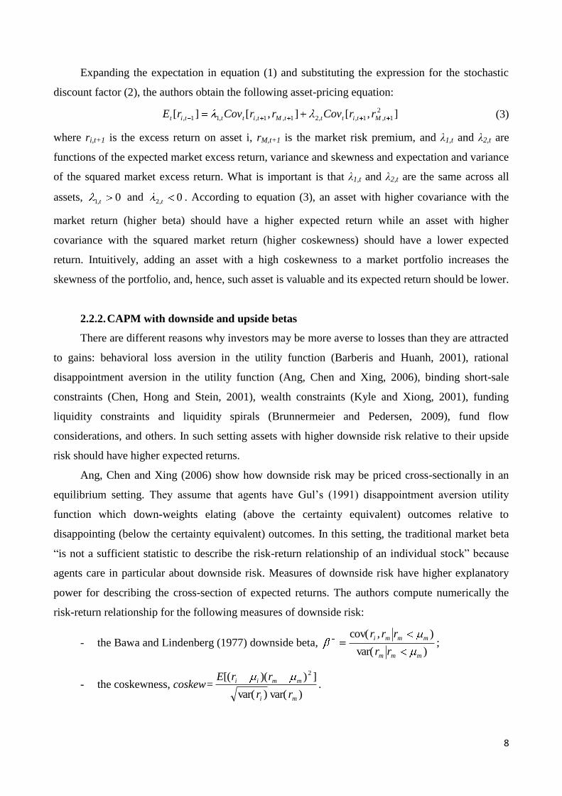
Expanding the expectation in equation (1) and substituting the expression for the stochastic

discount factor (2), the authors obtain the following asset-pricing equation:

],[],[][ 2

1,1,,21,1,,11, tMtitttMtitttit rrCovrrCovrE (3)

where ri,t+1 is the excess return on asset i, rM,t+1 is the market risk premium, and λ1,t and λ2,t are

functions of the expected market excess return, variance and skewness and expectation and variance

of the squared market excess return. What is important is that λ1,t and λ2,t are the same across all

assets, 0,1 t and 0,2 t . According to equation (3), an asset with higher covariance with the

market return (higher beta) should have a higher expected return while an asset with higher

covariance with the squared market return (higher coskewness) should have a lower expected

return. Intuitively, adding an asset with a high coskewness to a market portfolio increases the

skewness of the portfolio, and, hence, such asset is valuable and its expected return should be lower.

2.2.2. CAPM with downside and upside betas

There are different reasons why investors may be more averse to losses than they are attracted

to gains: behavioral loss aversion in the utility function (Barberis and Huanh, 2001), rational

disappointment aversion in the utility function (Ang, Chen and Xing, 2006), binding short-sale

constraints (Chen, Hong and Stein, 2001), wealth constraints (Kyle and Xiong, 2001), funding

liquidity constraints and liquidity spirals (Brunnermeier and Pedersen, 2009), fund flow

considerations, and others. In such setting assets with higher downside risk relative to their upside

risk should have higher expected returns.

Ang, Chen and Xing (2006) show how downside risk may be priced cross-sectionally in an

equilibrium setting. They assume that agents have Gul‟s (1991) disappointment aversion utility

function which down-weights elating (above the certainty equivalent) outcomes relative to

disappointing (below the certainty equivalent) outcomes. In this setting, the traditional market beta

“is not a sufficient statistic to describe the risk-return relationship of an individual stock” because

agents care in particular about downside risk. Measures of downside risk have higher explanatory

power for describing the cross-section of expected returns. The authors compute numerically the

risk-return relationship for the following measures of downside risk:

- the Bawa and Lindenberg (1977) downside beta, )var(

),cov(

mmm

mmmi

rr

rrr;

- the coskewness, coskew=)var()var(

]))([( 2

mi

mmii

rr

rrE.

9

They show that the traditional CAPM alpha is increasing in the downside beta and is decreasing in

coskewness. This means that assets should have higher expected returns if they have higher

downside betas and lower coskewness, because such assets perform poorly in bad states of the

world when the marginal utility of wealth is high. Assets with high upside betas are, on the

contrary, attractive and should have lower expected returns, ceteris paribus. Since the marginal

utility of wealth decreases when the overall market goes up (concave utility function), the upside

beta is not as important risk measure as the downside beta.

2.3. Data and portfolio formation

The data covers the period from January 1990 until April 2009 at a monthly frequency.

Earlier years are not analyzed due to the predominance of fixed exchange rate regimes and capital

controls in many developing countries in the sample. The sample of countries consists of 42

developed and emerging economies. Compared to Burnside‟s (2012) sample of 20 countries, my

sample includes many emerging market economies, some of which are popular targets of carry

trades because of their very high local interest rates. I also consider a sub-sample of 15 developed

countries. The full list of countries is provided in appendix 1.

I take a perspective of a US investor in order for my results to be comparable to those in

Lustig and Verdelhan (2007) and Burnside (2012). For each country, I collect the spot and forward

exchange rates against the US dollar. An increase in the exchange rate means an appreciation of the

respective currency against the US dollar. The exchange rate data is corrected for denominations

and periods of the fixed exchange rate regimes are dropped out because, otherwise, the currency

risk would be artificially lower.

The US non-durable real consumption is used to calculate the consumption risk, and the

MSCI all-country (AC) World index is used to calculate the stock market risk of currency

portfolios. This index aggregates the stock market performance in 45 countries. I use the global

stock market index as a proxy for the market portfolio because the main carry trade investors are

institutional investors which invest globally4.

The sources of data are Datastream and the Global Financial Database. I also collect data on

NYSE stock returns from CRSP.

Following Lustig et al. (2011), I sort currencies by the forward discount and form 5, 10 and

25 equally weighted currency portfolios in order to consider different levels of diversification

within portfolios. The portfolios are rebalanced monthly. When the covered interest parity is

4 The global market index has the correlation coefficient of 0.89 with the US stock market index, and considering the

US stock market index instead does not affect the results (not reported).

10

satisfied, the forward discount is approximately equal to the interest rate differential. Hence,

portfolio 1 always consists of currencies with the lowest local interest rates, portfolio 2 consists of

the next basket of currencies in the ranking, and portfolios 5, 10 and 25 always contain currencies

with the highest interest rates. Obviously, 5 portfolios are mostly diversified, while 25 portfolios are

rather noisy. The monthly rebalancing ensures that the portfolios resemble carry trade portfolios,

the composition of which changes over time as the forward discounts change. It should be noted

that currencies do move across portfolios quite often.

I also form the HML portfolio which has a long position in portfolio 10 (or 5, in case of 5

portfolios) and a short position in portfolio 1. This portfolio can be considered as the most

aggressive carry trade strategy, because it exploits the highest interest rate differential.

For the sub-sample of developed countries, the 15 currencies are sorted by the forward

discount into 5 portfolios. These portfolios are analyzed in sections 3.3 and 4.2.1.

3. RESULTS

3.1. Return and risk characteristics of currency portfolios

Figure 1 illustrates the relationships between the average excess returns to 10 currency

portfolios and their traditional, downside and upside betas. Here, all betas are estimated by OLS,

and the downside and upside betas are estimated in the following time-series regression with a

dummy variable:

mttjmtjjjt rdummyrr *

where jtr is total return of portfolio j, mtr is the global stock market return,0,1

0,0

mt

mt

tr

rdummy , j

is the estimate of the downside beta, and jj is the estimate of the upside beta. As here defined,

the downside beta measures the sensitivity of an asset‟s return to the market return in the states

when the market return is negative. Other cut-off levels for the downside beta are considered in

section 4.1.

[Figure 1]

Figure 1 shows that the spread of the downside betas (the middle panel) across portfolios is

wider than the spread in the traditional betas (the top panel), and the downside betas have greater

explanatory power in the cross-section of portfolio returns. There is insignificant negative

relationship between the upside betas (the bottom panel) and portfolio returns. The downside and

upside betas do not have symmetric relationship with portfolio expected returns, as the theoretical

11

model of Ang, Chen and Xing (2006) predicts. Hence, separating the beta into its upside and

downside components should improve the validity of the CAPM in the currency market.

Table 1 presents the returns and various risk characteristics of these 10 currency portfolios5.

The first row shows the average annualized excess returns of the portfolios. Although portfolios of

higher rank do seem to depreciate more against the US dollar than the lower-rank portfolios, the

exchange rate depreciation does not offset the gain from the interest rate differential, as predicted by

the UIP, so that the total portfolio excess returns are generally increasing with the portfolio rank.

The HML portfolio, the most aggressive carry trade portfolio which involves investments in high-

interest high-inflation emerging markets, generated the average return of 23.7 percent per annum

during the studied period6. This illustrates the profitability of carry trades.

[Table 1]

Portfolios of higher rank have higher return standard deviation and lower skewness7.

Although the relationship between portfolio returns and skewness is not completely monotonic,

generally it confirms the findings of Brunnermeier et al. (2008). The seven currencies considered in

Brunnermeier et al. (2008) are in portfolios 1-5, and I show that the negative relationship between

currency returns and skewness is more general in a bigger sample of developed and emerging

economies.

The subsequent rows of Table 1 show the efficient GMM estimates of consumption and

market betas of the currency portfolios8. The portfolio betas and beta premiums are estimated

jointly by GMM using a similar system of moment conditions as in Cochrane (2005):

0)(

0)(

0)(

jjt

ttjjjt

tjjjt

brE

ffbarE

fbarE

(4)

wheretf is either a factor or a vector of factors, jtr is the excess return on portfolio j, bj is a factor

beta, λ is a risk premium and γ is a constant (pricing error). The first two moments estimate factor

betas of each portfolio, and the third moment estimates the factor risk premium. I use both the

5 The characteristics of 5 and 25 portfolios have the same pattern and are not reported.

6 Returns do not take into account transaction costs.

7 If instead of rebalancing the portfolios monthly, I sort currencies just once, I do not find any relationship between the

portfolio rank and skewness. 8 The efficient GMM estimates of betas in Table 1 are not exactly the same as the OLS estimates in Figure 1 because of

the joint estimation of betas and beta premiums using the efficient weighting matrix. The OLS estimates are generally

higher and more statistically significant. They are available upon request

12

efficient and the identity weighting matrices in the estimation, but table 1 reports only the efficient

GMM estimates, and the first-step GMM estimates are very similar.

The consumption betas of all portfolios are statistically insignificant, which confirms the

Burnside‟s criticism of the relevance of the consumption CAPM for the currency market. The

downside consumption betas of all portfolios are much higher and statistically significant, although

the spread in them across portfolios is still insignificant to account for the cross-section of returns.

The stock market betas are increasing with the portfolio rank from 0.08 for portfolio 1 to 0.21

for portfolio 10. They are all statistically significant, but very similar across portfolios to explain the

differences in the portfolio returns.

The downside market betas are also increasing with the portfolio rank from 0.02 for portfolio

1 to 0.40 for portfolio 109. The spread in the downside betas across portfolios is much wider than

the spread in the traditional betas. The downside betas are close to zero and statistically

insignificant for portfolios 1 and 2, which means that these portfolios are immune to the stock

market downturns and can serve as a „safe haven‟. Portfolios 9 and 10, on the contrary, have high

and statistically significant downside betas, which means that these portfolios have significantly

negative returns in the bad states of the world. The downside betas of these portfolios are almost

twice as high as their traditional betas. Therefore, while the average covariance of the high-interest

currencies with the market is modest, it rises significantly during the market downturns. Hence,

carry trades tend to crash exactly when the stock market goes down.

Unlike the downside betas, the upside betas are decreasing with the portfolio rank. When the

stock market goes up, the low-interest currencies tend to provide higher returns than the high-

interest currencies. Although the upside betas of almost all portfolios are statistically significant,

they are not much different from each other.

Figure 3 shows the relationship between the traditional market betas, the downside betas and

the upside betas of the 10 currency portfolios. Because the downside betas are increasing with the

portfolio rank and the upside betas are decreasing, and because the traditional betas are the

weighted averages of the downside and the upside betas, the pattern of traditional betas across

portfolios is rather flat. The traditional market betas cannot explain the returns to carry trades

because they are not informative about the actual risks of the currency portfolios. By separating the

traditional beta into the upside beta and the downside beta, we obtain much more information about

the performance of the carry trade portfolios.

9 If the currencies are sorted into portfolios by their downside betas instead of the forward discounts, the similar

monotonic relationship between the downside betas and portfolio returns is observed.

13

The last row of table 1 reports coskewness of portfolio returns with the global stock market,

which is estimated in a time series regression of returns on squared market returns. Similarly to

skewness, coskewness is positive for portfolio 1, is almost monotonically decreasing with the

portfolio rank and is significantly negative for the high-interest portfolios. A significant negative

coskewness indicates that a portfolio has negative returns in periods of high stock market volatility,

and investing in such a portfolio increases the crash risk for the investor. The same conclusion has

been drawn in Menkhoff et. al (2012a), Ronaldo et al. (2009) and Clarida et al. (2009) by looking at

conditional currency returns using different proxies for volatility. But coskewness as a measure of

risk has not been analyzed previously in the currency literature.

According to the three-moment CAPM, it is the coskewness which is important for a

diversifying investor, rather than nonsystematic skewness. The close relationship between skewness

and coskewness of the ten currency portfolios indicates that if a currency portfolio crashes, it

crashes in periods of high stock market volatility. But high stock market volatility is usually

observed on the downside. Therefore, the coskewness and the downside beta can be considered as

alternative measures of the downside market risk. Indeed, the downside betas are strongly

correlated with the coskewness across portfolios (the correlation coefficient -0.999) and it is hard to

separate them from each other.

Overall, Table 1 suggests that the high returns to carry trades is a compensation for their high

downside market risk, which cannot be diversified away because the market portfolio performs

poorly in such states. This hypothesis is tested formally in the next section.

3.2. Downside risk pricing in the currency market

In this section I test the validity of alternative asset pricing models for the cross-section of 10

currency portfolios of developed and developing countries. I consider the following models:

consumption CAPM, consumption CAPM with the downside beta, CAPM, downside beta CAPM,

upside beta CAPM and coskewness CAPM.

The models are estimated by GMM, using the moment conditions in (4). GMM minimizes the

weighted sum of these moments, and the covariance matrix between the two sets of moments

captures the effect of generated regressors on the standard errors of the risk premiums. The GMM

estimation is preferable to the commonly used in the literature Fama-MacBeth two-step procedure,

because the GMM standard errors of the coefficients account for the fact that the betas are

generated regressors. Following the Fama-MacBeth procedure, we are more likely to falsely accept

the model, because the standard errors are generally lower. This is one of Burnside‟s (2011) major

14

criticisms of Lustig and Verdelhan‟ (2007) test of the consumption CAPM model. Burnside shows

that once the standard errors are estimated properly using the GMM, the consumption risk premium

for the currency portfolios is insignificant and, hence, the consumption risk is not priced.

For each specification, I estimate both the first-step GMM with the identity weighting matrix

and the iterated GMM with the efficient weighting matrix, which assigns more weight to the

moments which are estimated more precisely.

The GMM estimates of the risk premiums and various fit statistics for the alternative

specification are reported in table 2.

[Table 2]

First, the consumption CAPM is rejected on all grounds. Not only the consumption betas in

table 1 are insignificant, the consumption beta premiums are all statistically insignificant too (as in

Burnside, 2011). The model is also rejected by the test for the overidentifying restrictions in case of

the identity weighting matrix, and the mean sum of squared errors (MSSE) is higher than for some

other models. The consumption CAPM with the downside consumption betas performs better in

terms of the overall fit of the model. But the downside consumption risk premiums are still

statistically insignificant. Non-durable consumption is just not volatile enough for the consumption

betas to be measured precisely, and consumption betas cannot account for the cross-sectional spread

of carry trade returns.

Second, the upside beta CAPM is also rejected. The upside beta premiums are negative and

statistically insignificant. This goes in line with the predictions of Ang, Chen and Xing (2006)

model, that in the good states of the world, the marginal utility of wealth is low, and assets which

perform well in such states are not particularly valuable.

Third, the traditional beta premiums, the downside beta premiums and the coskewness

premiums are all statistically significant and have the correct signs, all intercepts are close to zero

and the three models are not rejected by the T*J statistics. Therefore, the market risk is priced in the

currency market.

Forth, the downside beta CAPM wins the horse race. Comparing the CAPM and the downside

beta CAPM, the downside beta premium is about three times as low as the beta premium because

the spread in the downside betas across the currency portfolios is about three times as wide as the

spread in betas. As Lewellen, Nagel and Shanken (2010) point out, to make the correct judgment

about an asset-pricing model, we should look not only at the statistical significance of risk

premiums, but also at their magnitude and economic meaning. Whereas the estimates of the

15

traditional beta premium are 10-19 percent, the estimates of the downside beta premium are 4-6

percent, which is closer to the average market excess return in this period. Also, the downside beta

premium is measured more precisely and the MSSE is lower. The coskewness premium is also

highly significant, but the coskewness CAPM has higher MSSE. Therefore, the downside beta

CAPM fits the data better than other models. The high returns to carry trades are just a

compensation for their high downside market risk.

Lustig et al. (2011) propose two factors – EW (level) and HML (slope) – to explain the

returns to the currency portfolios. They show that the currency portfolios, sorted by the forward

discounts, load differently on the HML factor, and the spread of these loadings accounts for the

spread of the portfolio returns. But the HML portfolio itself has high loading on the downside

market factor. For example, the HML strategy considered in this paper (10-1 portfolio) has the

downside beta of 0.38 and highly statistically significant. Because higher-interest currency

portfolios load more on the downside market factor, they load more on the HML factor. The two

factors are closely linked, and their explanatory power in the cross-section regressions is similar.

See section 3.4 for the „horse races‟ between alternative factors.

My findings go at odds with Burnside‟s (2012) claim that the stock market risk cannot explain

the returns to carry trades. He argues, that the market betas of carry trade portfolios are too small to

rationalize their high returns, and once a traditional market-risk-based model is estimated for

currency and stock portfolios together, it is rejected due to high pricing errors for the currency

portfolios. Why do I arrive at the opposite conclusion to Burnside‟s (2012)?

Let us consider his first reason first. Burnside has a much smaller sample of countries than

mine (he does not consider many emerging countries which I consider), and forms only two carry

trade portfolios: EW is an equally-weighted portfolio of all currencies and HML is a portfolio with

long positions in 20% of the highest-interest currencies and short positions in 20% of the lowest-

interest currencies. His EW portfolio would be similar to an equally-weighted combination of my

10 portfolios, and his HML portfolio is similar to my HML portfolio by construction except for the

fact that we have different currencies in our HML portfolios. His OLS estimates of the market betas

of EW and HML portfolios are 0.03 (insignificant) and 0.16 (significant), respectively. My OLS

estimates of the market betas are higher, especially for the HML portfolio (0.2610

), because my

HML portfolio has a long position in high-interest emerging countries which Burnside does not

consider. In fact, Burnside‟s HML portfolio is similar by its characteristics to my “9-1” portfolio

10

The OLS estimates are only shown in Figure 1. They are available upon request.

16

which has a long position in portfolio 9 and a short position in portfolio 1. But once we consider

more emerging countries, the market risk of the HML carry trade strategy is higher.

Moreover, if we measure the market risk on the downside, it is higher for the high-interest

currencies and lower for the low-interest currencies, so that the spread is much wider. The OLS

downside beta of my “9-1” portfolio is 0.31 and that of my HML portfolio is 0.58. So, the market

risk of carry trades is almost twice as high, when measured on the downside.

Now let us consider Burnside‟s second reason. He does not estimate the asset-pricing models

for currency portfolios because he has only two portfolios. Instead, he estimates the models for 25

Fama-French portfolios plus the two currency portfolios. I believe that this is an inappropriate

exercise. Even in case of the identity weighting matrix, the weight of the stock portfolios is much

higher (25/27) than the weight of the currency portfolios (2/27) in the estimation. So, the models are

in fact estimated for the stock portfolios, and then he checks whether the currency portfolios „fit‟

these models. But we know that the Fama-French portfolios can be priced by the Fama-French

factors. Not surprisingly, he finds that the Fama-French model is the only model which is not

rejected. But why would the Fama-French factors price the currency portfolios? They would not,

and he finds that the pricing errors are significant indeed11

. Therefore, Burnside concludes, that

“there is no unifying risk based explanation of returns in these two markets”.

In this section, I show that the asset pricing models with downside market risk fit the cross-

section of currency portfolio returns well. In the next section, I estimate the same models for the

currency and stock portfolios together, and I arrive at the same conclusion. I just treat the currency

and stock portfolios equally and use more comparable sets of portfolios.

3.3. Comparison of currency and stock markets

Is the downside risk priced similarly in the currency and stock markets? The efficient GMM

estimate of the downside risk premium is 6 percent for the 10 currency portfolios of developed and

developing countries. Regarding the evidence from the stock market, Ang, Chen and Xing (2006)

estimate the downside beta premium between 2.8 and 6.9 percent (statistically significant) in the

Fama-MacBeth (1973) regressions for individual NYSE stock returns during 1963-2001. But the

Fama-MacBeth estimates are not directly comparable to the efficient GMM estimates. Therefore, I

estimate the market risk premiums for currency and stock portfolios jointly by GMM. But instead

of considering the Fama-French portfolios, as in Burnside (2012), I consider stock portfolios sorted

11

The efficient GMM makes the „fit‟ of the currency portfolios even worse because it attaches even higher weight to the

stock moments which are measured more precisely.

17

by the downside beta, because these portfolios have clear downside risk-return relationship (Ang,

Chen and Xing, 2006), while other risks are diversified away within the portfolios.

I collect monthly total return data for all NYSE stocks for the period from January 1990 until

December 2008 from CRSP. Following Ang, Chen and Xing (2006), I restrict the sample to NYSE

stocks to minimize the illiquidity effect of small firms12

. Stocks with less than 25 time series

observations are excluded from the sample due to the low number of observations to estimate the

downside beta properly. This leaves me with 3,349 stocks in the sample.

The stock portfolios are formed as follows. For each stock, I estimate its downside market

beta in a 5-year rolling window. Every month, all stocks are sorted by their downside betas,

estimated prior to the sort date, into 5 equally-weighted portfolios. Portfolio 1 always contains 20

percent of stocks with the lowest pre-ranking downside betas and portfolio 5contains20 percent of

stocks with the highest downside betas. Since the number of stocks in the sample is very large, all

portfolios are highly diversified, and this sorting procedure allows concentrating on the downside

risk of the portfolios.

I consider two sets of currency portfolios. The first set includes 5 currency portfolios of

developed and developing countries, sorted by the forward discount. These portfolios are formed

from the same currencies as in the previous section, but they are more diversified. Each portfolio

consists of seven currencies, on average. The second set of 5 portfolios is formed from currencies of

developed countries only. The portfolios are sorted by the forward discount. Each portfolio consists

of three currencies, on average.

I estimate alternative asset pricing models for 5 currency and 5 stock portfolios together13

,

using the moment conditions (4). It is important to have the same number of currency and stock

portfolios in the estimation, so that the first-step GMM treats currencies and stocks equally a priori.

Then the efficient GMM will amend the weights, but they will be based on asset-pricing

considerations.

Table 3 reports the efficient GMM estimates of risk premiums and various test statistics for

the downside beta CAPM, the coskewness CAPM and the traditional CAPM for 5 currency and 5

stock portfolios. The first-step GMM estimates are very similar and are not reported.

[Table 3]

12

Ang, Chen and Xing (2006) show that the validity of the downside beta is confirmed in a wider sample of NYSE,

AMEX and NASDAQ firms. 13

I also estimated the models for 10 currency and 10 stock portfolios, sorted in the same manner. The results are very

similar and are not reported.

18

No matter which set of currency portfolios is used (all countries or developed countries only),

the results are very similar. The downside beta premium, the traditional beta premium and the

coskewness premium are all highly statistically significant. None of the models is rejected by the

test for the overidentifying restrictions. The MSSE for the currency moments are even lower than

the errors in table 2. Hence, adding stock portfolios does not worsen the fit of the models. But the

MSSE for the stock moments are all higher due to generally higher volatility of stock returns. The

downside beta CAPM and the coskewness CAPM have lower T*J statistics and MSSE than the

traditional CAPM, and hence they are superior for both currency and stock portfolios.

The downside beta premium, estimated for the currency and stock portfolios jointly (2

percent), is lower than the downside beta premium estimated for the currency portfolios in table 2

(6 percent)14

. Although the downside risk is priced in the both markets, the price of risk seems to be

higher in the currency market. This can be a consequence of underpricing of the currencies of high-

interest emerging economies. These currencies have too high returns relative to their downside

betas and drive the downside beta premium upwards15

. But if we consider currencies of developed

countries only, the estimate of the downside beta premium is lower (1 percent). A more detailed

analysis of currencies of developed countries is presented in section 4.2.1.

Figure 2 plots the downside risk-return relationship for 5 currency (triangles) and 5 stock

(round dots) portfolios. Currencies of all countries are plotted in the top panel and currencies of

developed countries are plotted in the bottom panel. We see that portfolio C5 in the top panel,

which consists of currencies of high-interest emerging markets, is an outlier. Once we exclude this

portfolio or restrict the sample of currencies to developed countries, the currency and stock

portfolios lie closely to the security market line with very high R2.

[Figure 2]

The same conclusion can be drawn for the coskewness CAPM. Apart from portfolio C5 in the

top-right panel, all other currency and stock portfolios satisfy the same coskewness-return

relationship.

14

The same applies to coskewness. 15

Why don‟t capital flows eliminate this underpricing? These countries have very high country risk, measured by Fitch

sovereign rating (see appendix 2). There is a lot of uncertainty associated with investments in these currencies, in some

cases there were (are) explicit or implicit capital controls and insufficient liquidity. Institutional investors may set

country limits to prevent position-taking in currencies of high-risk countries and hence, country risk is a natural limit to

arbitrage. Menkhoff et al. (2012b) find that high country risk may be a reason why arbitrageurs do not also fully exploit

high currency momentum returns.

19

Overall, the currency portfolios have lower downside risk (lower downside betas and higher

coskewness) and lower expected returns than the stock portfolios, but the downside risk premiums

in the currency and stock markets are similar. We just cannot reject the hypothesis, that the

downside risk is priced similarly in the currency and stock markets.

Is the risk premium of 1-2 percent per month a fair compensation for the downside risk?

According to the traditional CAPM, the expected market excess return is a fair compensation for the

overall market risk. According to the Kahneman and Tversky (1979) prospect theory, people are

approximately 2.5 times more averse to losses than to gains, and hence we may expect the downside

risk premium to be about 2 times higher. Since the market excess return was about 6 percent per

annum during the studied period, the fair downside risk premium should be about 12 percent per

annum.

Another approach to identify the fair downside risk premium is to construct the downside

market factor-mimicking portfolio. The risk price of the factor should be equal to the mean return

on this traded portfolio so that the no-arbitrage condition is satisfied. I follow the two-step

methodology of Breeden et al. (1989) and Menkhoff et al. (2012a). First, I regress the downside

market factor on the five currency portfolio excess returns and obtain the betas16

. Then I use the

betas as the weights of the currency portfolios to construct the factor-mimicking portfolio. The

average annual return to this factor-mimicking portfolio is 11 percent.

The two approaches suggest that the fair downside risk price is about 1 percent per month,

and this is what I find in the cross-section of developed currencies and stock portfolios. Therefore,

the high returns to carry trades are a fair compensation for their high downside market risk.

However, currencies of emerging markets provide a higher risk premium perhaps due to the limits

to arbitrage involved in trading these currencies.

3.4. ‘Horse races’ between alternative factors

In this paper I claim that the downside market factor (or the downside beta) and market

volatility factor (or the coskewness) both can explain the cross-section of carry trade returns well.

The two factors are highly correlated (the correlation coefficient is -0.71) and it is difficult to

separate their effects, because high market volatility is usually observed on the downside.

Therefore, I consider the both factors as the downside risk factors.

Among other risk factors which have proved to have high explanatory power for carry trades

are the Lustig et al. (2011) HML factor and the Menkhoff et al. (2012a) global currency volatility

16

These betas are monotonically increasing in the portfolio rank.

20

innovation factor. These two factors are derived from currency returns themselves and are both

highly correlated with the second principal component of carry trade portfolios, which is shown to

explain a great proportion of currency return variance.

In this section I ran „horse races‟ between the four alternative factors in one-factor and

multifactor settings. I use my own HML factor, which is a little bit different from the Lustig et al.

(2011) HML factor due to the different samples of countries, and I use Menkhoff et al. (2012a)

currency volatility factor (VOL).

First of all, the currency factors (HML and VOL) are not highly correlated with the downside

market factor and the market volatility factor (the correlation coefficient is 0.35-0.39 by the

absolute value). The second principal component (which together with the first principal component

explains 91% of variance) has the highest correlation with the HML factor17

and the lowest

correlation with the VOL factor. The market factors are in between.

I also construct the factor-mimicking portfolios for the downside market factor, the market

volatility factor and the currency volatility factor by regressing each factor on the five currency

portfolio returns, and using the obtained betas as the weights of the currency portfolios in the factor-

mimicking portfolios. Interestingly, the three factor-mimicking portfolios are almost perfectly

correlated (the correlation coefficient is 0.99 by the absolute value), because the currency portfolios

load similarly on the factors (portfolio 1 has the lowest loading on the factors and portfolio 5 has the

highest loading). The second principal component correlates similarly with the three factor-

mimicking portfolios.

Table 4 reports the efficient GMM estimation results for the five portfolios of all currencies18

.

I columns 1-4 I compare one-factor models. All four factors are highly statistically significant, their

premiums have the correct signs, all intercepts are statistically insignificant, and none of the models

is rejected by the T*J-statistics. So, all factors are doing well in explaining the currency returns. But

the model with the HML factor has the lowest MSSE, and the model with the market volatility

factor has the lowest T*J-statistics. The currency volatility factor, on the contrary, has the highest

MSSE and T*J-statistics, hence, this factor provides the greatest pricing errors.

[Table 4]

17

This is not surprising given that they are constructed in approximately the same way. 18

The results for the 10 portfolios of all currencies, for the 5 portfolios of currencies of developed countries, and for the

5 currency and 5 stock portfolios are similar.

21

In columns 5-9 I consider two-factor specifications and in columns 10-11 three-factor

specifications. When both the downside market factor and the market volatility factor are included

(column 5), none of them loses the statistical significance. Since the two factors are highly

multicollinear, it is difficult to disentangle their effects. The downside beta premium falls from 7 to

4 percent and is closer to the theoretical value.

When I consider the downside market factors and the VOL factor (columns 6, 8 and 10), the

market factors remain significant (at 10 percent level) while the VOL factor does not. The VOL

premium even becomes positive. Whereas the VOL factor alone can explain the carry trade returns,

its explanatory power is swiped off by the downside market factors. Menkhoff et al. (2012a)

provide ample evidence in favour of their currency volatility factor, but they never control for the

market factors in their specifications.

When I consider the downside market factors and the HML factor (columns 7, 9 and 11), the

HML factor remains significant, while the downside market factor and the market volatility factor

become insignificant19

. Menkhoff et al. (2012a) also find that the VOL factor becomes insignificant

when they control for the HML factor. So, the HML factor has the highest appeal to explain the

currency returns. But the HML factor is not “exogenous” to these portfolios, it is constructed form

these portfolios in the first place. Therefore, it is not surprising that it has such a high explanatory

power.

Unfortunately, the HML factor cannot be considered as a unifying risk factor because it does

not price stock portfolios. Table 5 shows the efficient GMM estimates for the 5 stock portfolios

considered in the previous section. Although none on the factors is rejected by the T*J-statistics,

only the downside market factor and the market volatility factor are statistically significant. The

HML and the VOL factors do not have significant explanatory power in the stock market. Burnside

(2012) also finds that the HML factor (and other currency factors) cannot explain the returns to the

25 Fama-French portfolios sorted on size and value.

[Table 5]

While the currency factors (HML and VOL) have high explanatory power in the currency

market, they have low explanatory power in the stock market. But the downside market factors have

high explanatory power in the both stock and currency markets. Lettau et al. (2013) also show the

validity of the downside market risk in the bond and commodity markets. The downside market

19

The same holds if the factor-mimicking portfolios are used instead of the factors themselves.

22

factors also have theoretical grounds, as discussed in section 2.2. Therefore, the downside market

risk wins the „horse race‟ and can be considered as a unifying explanation of returns in various asset

markets.

4. ROBUSTNESS TESTS

4.1. Extreme downside risk and disaster risk

In the previous sections, the downside betas are estimated conditioning of the market return

being negative. Another common way to estimate downside betas in the literature is to condition on

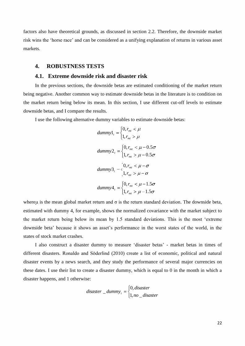
the market return being below its mean. In this section, I use different cut-off levels to estimate

downside betas, and I compare the results.

I use the following alternative dummy variables to estimate downside betas:

mt

mt

tr

rdummy

,1

,01

5.0,1

5.0,02

mt

mt

tr

rdummy

mt

mt

tr

rdummy

,1

,03

5.1,1

5.1,04

mt

mt

tr

rdummy

where is the mean global market return and σ is the return standard deviation. The downside beta,

estimated with dummy 4, for example, shows the normalized covariance with the market subject to

the market return being below its mean by 1.5 standard deviations. This is the most „extreme

downside beta‟ because it shows an asset‟s performance in the worst states of the world, in the

states of stock market crashes.

I also construct a disaster dummy to measure „disaster betas‟ - market betas in times of

different disasters. Ronaldo and Söderlind (2010) create a list of economic, political and natural

disaster events by a news search, and they study the performance of several major currencies on

these dates. I use their list to create a disaster dummy, which is equal to 0 in the month in which a

disaster happens, and 1 otherwise:

disasterno

disasterdummydisaster t

_,1

,0_

23

The economic disasters include famous financial crises, defaults or bankruptcies, the political

disasters include wars, terrorism and bombings, and the natural disasters include hurricanes,

tornado, tsunami and earthquakes. The full list of disasters and the dates is provided in appendix 3.

Table 6 reports the efficient GMM estimates of the „extreme downside betas‟ and „disaster

betas‟, estimated with dummy 4 and disaster dummy, respectively (panel A)20

, and the estimates of

the alternative downside beta premiums and the „disaster beta‟ premium (panel B).

[Table 6]

The „extreme downside betas‟ are all higher than the downside betas in table 1, and they are

all highly statistically significant. The „disaster betas‟ are even higher. Therefore, the carry trades

perform disproportionally worse in the states of stock market crashes or disasters. But even the low-

interest currency portfolios have statistically significant „extreme downside betas‟ and „disaster

betas‟. It means that all currencies generally depreciate against the US dollar in times of the global

market crashes or disasters. This confirms the „safe haven‟ properties of the US dollar as a reserve

currency, documented by Maggiori (2011).

Turning to panel B, all downside beta premiums and the „disaster beta‟ premium are highly

statistically significant and very similar to each other and to the downside beta premium in table 2.

All specifications have very similar test statistics. The intercepts are statistically significant in cases

of dummy 4 and disaster dummy, reflecting the „safe haven‟ properties of the dollar in times of the

extreme stock market downturns or economic, political or natural disasters. This intercept reflects

the „dollar safety premium‟.

Overall, varying the cut-off level for the downside beta and considering the „disaster beta‟ as

an alternative risk measure does not change the result that carry trades perform poorly in states of

high marginal utility of wealth, and the high returns to carry trades are a compensation for this.

4.2. Other sets of currency portfolios

4.2.1. Sub-sample of developed countries

I study a sub-sample of developed countries separately for two reasons. First, some of the

emerging countries may not have had sufficiently liquid futures market in the earlier years or some

currencies were pegged to the US dollar, and hence their exchange rate risks were artificially lower.

20

The downside betas estimated with dummies 1, 2 and 3 are similar to the ones in table 1 and are not reported.

24

Therefore, the downside beta premium, obtained for the whole sample, may be overestimated.

Secondly, the most popular carry trade currencies are still currencies of developed countries, and

institutional investors limit their exposure to emerging markets despite their high returns. Again, the

downside risk premium, obtained for the whole sample, may be higher than in other markets

because of such limits to arbitrage. Easily-accessible currencies of developed countries are better

test assets for the comparison of the currency and stock markets, as shown in section 3.3.

Table 7 presents the return and risk characteristics of 5 currency portfolios (panel A) and the

efficient GMM estimates of various risk premiums (panel B). Portfolios of higher rank have higher

returns and return standard deviations and somewhat lower (negative) skewness. However, the

pattern of skewness is non-monotonic, as for the whole sample. The efficient GMM estimates of the

consumption betas and the downside consumption betas are all statistically insignificant. The

consumption betas are even decreasing in the portfolio rank. The consumption beta premium and

the downside consumption beta premium are both statistically insignificant. There is no evidence

that the consumption risk can explain the cross-section of these currency portfolio returns.

[Table 7]

All global stock market betas (the traditional beta, the downside beta, the „extreme downside

beta‟, the „disaster beta‟ and the upside beta) are monotonically increasing with portfolio rank from

close to zero and insignificant values for portfolio 1 to rather high and significant values for

portfolio 5. The spread in the market betas across the portfolios is highly significant. If we look at

“5-1” HML portfolio, its market beta is 0.18, its downside beta is 0.23, its „extreme downside beta‟

is 0.26 and its „disaster beta‟ is 0.41.

These values are lower than in case of 10 portfolios of all currencies, except for the „disaster

beta‟. The „disaster beta‟ is higher here because portfolio 1 of currencies of developed countries

has lower „disaster beta‟ than portfolio 1 of all currencies. In times of economic, political and

natural disasters all currencies generally depreciate against the US dollar, except for the low-interest

currencies of developed countries (e.g. the Japanese yen or the Swiss franc). Therefore, the US

dollar and the low-interest currencies of other developed countries possess the „safe haven‟

properties (as in Ronaldo and Söderlind, 2010). But the „disaster betas‟ of high-interest currencies

of developed countries are comparable in magnitude to the „disaster betas‟ of high-interest

currencies of developing countries (portfolios 9 and 10). Hence, no matter which sample of

currencies we consider, carry trades crash in times of disasters or stock market downturns.

25

Whereas the traditional beta premium is insignificant (panel B), the downside beta premium

and especially the „extreme downside beta‟ premium and the „disaster beta‟ premium are

statistically significant. The downside risk premiums, obtained in the sub-sample of developed

countries, are lower in magnitude and similar to the premiums, obtained for the stock market. The

„extreme downside beta‟ CAPM and the „disaster beta‟ CAPM have the highest explanatory power

again.

The upside betas in table 7 are increasing in the portfolio rank, but the spread in them across

portfolios is not so significant. The upside beta premium is positive, but statistically insignificant as

before.

Although coskewness is decreasing in portfolio rank, it is statistically insignificant for all

portfolios, and the coskewness premium is insignificant too, unlike in case of all currencies. It

follows that currencies of developed countries are not prone to volatility risk, and the coskewness

CAPM cannot explain their returns.

4.2.2. 25 less-diversified portfolios of developed and developing countries

In this section I consider another set of currency portfolios – 25 portfolios, formed from all

currencies in the sample. These are also carry trade portfolios, but they are much less diversified

and hence are rather noisy. Each portfolio consists of 1.4 currencies, on average.

The market betas of these portfolios are not reported because the general patterns are the same

as for the 10 portfolios, considered previously. The consumption betas are all statistically

insignificant. All market betas are statistically significant, and they are monotonically increasing

with the portfolio rank. The market betas range from 0.04 to 0.25, the downside betas range from

0.04 to 0.37, and the coskewness ranges from -0.35 to -2.53 (all for portfolios 1 and 25,

respectively).

[Table 8]

Table 8 reports the efficient GMM estimates of risk premiums. All risk premiums have the

same signs as in case of 10 portfolios, are a little higher in magnitude and are highly statistically

significant. The traditional CAPM has implausibly high risk premium and higher MSSE. Therefore,

it loses the „horse race‟ to the models with downside risk. The models with downside risk have

more economically meaningful risk premiums and better overall fit.

26

4.3. Period of active carry trades by institutional investors: 2000-2009

Early 90s are the years of soaring interest rates, capital controls, political instability and the

related currency crashes in several emerging countries in the sample. This was reflected in the

extreme behavior of the top portfolios, such as their very high returns and high skewness. At the

end of 90s, after the financial crises in East Asia and Russia, the economic situation in most

emerging countries stabilized. Also we observed a tremendous growth of carry trade activities,

which started in late 90s (Galati et al., 2007) and continued until the financial crisis of 2008, when

they crashed. In this section I study the latest period from January 2000 until April 2009 – the

period of active carry trades.

Table 9 reports the return and risk characteristics of 10 portfolios of all currencies and 5

portfolios of currencies of developed countries (panel A), as well as the efficient GMM estimates of

risk premiums for the two sets of portfolios (panel B).

[Table 9]

All market betas and coskewness are highly statistically significant in the recent period. All

currencies co-vary stronger with the global stock market, especially on the downside, and this can

actually be a consequence of active institutional trading in currencies in the last decade, as the

model of Basak and Pavlova (2012) predicts. The market betas, the downside betas and the „disaster

betas‟ of the high-interest portfolios are higher now.

The increase in the market betas is greater for the high-interest portfolios of developed

countries, particularly if we consider the „extreme downside betas‟ (0.42 versus 0.26). The

coskewness of portfolio 5 also decreased significantly from -0.89 to -2.1 and became significant. A

carry trade strategy which involves only developed countries has significantly higher downside

market risk in 2000-2009.In fact, no matter which set of currencies we consider, the carry trade

long-short portfolios have similar downside market risk whereas, previously, the downside risk of

currencies of emerging markets was much higher. High-interest currencies of developed and

developing countries tend to crash equally in states of adverse stock market conditions or political

and natural disasters. This is the evidence of the „asset-class effect‟ in the currency market, since

these currencies are the most popular target currencies of carry traders. As Basak and Pavlova

(2012) show theoretically, assets which institutions trade exhibit a greater degree of co-movement.

As before, the spread in the downside betas is wider than the spread in the traditional betas

across the both sets of portfolios, and the spreads in the „extreme downside beta‟ and „disaster

27

betas‟ are even wider. The traditional beta premium and the coskewness premium are insignificant

in the sub-sample of currencies of developed countries, whereas the downside beta premium, the

„extreme downside beta‟ premiums and the „disaster beta‟ premium are statistically significant for

the both samples of currencies. None of the models is rejected by the test for the overidentifying

restrictions, but the downside beta CAPM, the „extreme downside beta‟ CAPM and the „disaster

beta‟ CAPM have the lowest mean sum of squared errors (MSSE).

As before, the estimates of the downside risk premium, obtained for the whole sample of

currencies, are higher than the estimates, obtained for the sub-sample of currencies of developed

countries. The price of downside risk is higher for the currencies of emerging markets, perhaps, due

to the limits institutions set for their exposure to emerging markets. Such limits and the high

sovereign risk of these countries prevent capital flows to arbitrage away the excess returns in the

emerging markets.

The estimate of the downside risk premium, obtained for the sub-sample of currencies of

developed countries, is similar to that in the stock market, 1-2 percent per month. This premium

makes economic sense. Therefore, the downside market risk is priced fairly in the currency market.

4.4. Time-varying market betas and Fama-MacBeth estimation

While in the previous sections betas were assumed constant in the sample, in this section, I

allow betas to vary over time. I follow the two-step Fama-MacBeth (1973) procedure where, in the

first step, betas are estimated in a five-year rolling window, and in the second step, the cross-section

regression of portfolio returns on betas in the preceding five years is estimated. Hence, this is an

out-of-sample test. I concentrate on the latest period from January 1999 until April 2009 when the

stock market risk of currency portfolios seems to be more important. Since the first set of betas is

estimated during the period from January 1999 until December 2003, the first cross-section

regression is run for January 2004. Then the rolling window moves by one month and the procedure

is repeated. This generates a time series of beta premiums, from which I find the average beta

premium and its statistics.

Lustig and Verdelhan (2011) find significant time variation of betas of their currency

portfolios, with betas increasing dramatically during crisis periods. I also find some variation in the

estimated upside and downside betas over time, although the overall pattern is more monotonic

(generally, all stock market betas have monotonically increased over time in the studied period).

The cross-section relationship of time-varying betas of 10 currency portfolios of developed

and developing countries is the same as before. The lowest-interest currency portfolio downside

28

beta is always negative with the average value of -0.08 and little time variation. The downside beta

of the highest-interest portfolio is always the highest in the cross-section with the average value of

0.59 and the maximum and minimum values of 0.79 and 0.18, respectively (OLS estimates). The

downside betas of all portfolios, except portfolio 1, increased significantly during the financial

crisis in October 2008 – April 2009, when carry trades crashed dramatically. There is a particularly

visible positive relationship between portfolio rank and the downside beta in this period.

In the Fama-MacBeth cross-section regressions for 10 currency portfolios, the downside beta

premium is 12 percent per annum with a t-statistic of 2.12, while the upside beta premium is -0.02

and insignificant, as before. The two betas explain 43 percent of portfolio excess returns, on

average, while the traditional beta explains only 32 percent of returns. Generally, the conclusion

that the downside market risk can explain the returns to carry trades is robust when betas are time-

varying and estimated by OLS.

5. CONCLUSION

In this paper, I look at the downside market risk of currencies as the explanation for the high

excess returns of carry trades, which have consistently been observed empirically, and due to which

the popularity of the strategy has increased dramatically among both institutional and private

investors. I study portfolios of currencies sorted by the forward discount to diversify away

idiosyncratic risk and to concentrate on those properties of currencies which are specific to

countries with different levels of interest rates.

I find that the market risk of currency portfolios is monotonically increasing in the level of the

local interest rate. The returns of high-interest (investment) currencies have significant negative

skewness and coskewness with the stock market, high downside stock market betas and high

downside consumption betas, while the returns of low-interest (funding) currencies, on the contrary,

have positive skewness and coskewness and insignificant downside betas. This suggests that returns

to carry trades are asymmetrically distributed with a high crash risk, and the crashes happen exactly

in the worst states of the world, when the stock market goes down significantly and the marginal

utility of wealth is high.

I run „horse races‟ between alternative asset-pricing models to explain the cross-section of

currency portfolio returns. I find that the downside market beta has a much greater explanatory

power than the traditional market beta, and that the coskewness is also highly significant. The

GMM estimates of the downside beta and coskewness premiums are highly significant, similar in

the currency and stock markets and close to the theoretical values. The downside risk is priced

29

similarly in different markets, and the high returns to carry trades are a fair compensation for their

high downside market risk.

The results are robust to the use of different sets of currency portfolios and different methods

of estimation, and they are even stronger if we consider the „extreme‟ downside risk and disaster

risk or the latest period of active carry trades. The downside risk of investment currencies is even

higher in the recent period, no matter whether these currencies belong to developed or developing

countries, and the explanatory power of the downside risk in the cross-section is greater. This

suggests that there is a closer link between the currency and stock markets now. The rising volume

of carry trade activity by institutional investors might have contributed to this trend. According to

the head of Britain‟s financial regulator Adair Turner, the carry trade could be destructive to some

economies, and “if the trades were reduced the world would be a better place”21

.

References

1. Ang, Andrew, Joseph Chen, and Yuhang Xing, 2006. Downside risk. Review of Financial

Studies, 19(4), 1191-1239.

2. Barberis, N., M. Huang, and T. Santos, 2001. Prospect theory and asset prices. Quarterly

Journal of Economics, 116, 1-53.

3. Basak, Suleyman, and Anna Pavlova, 2012. Asset prices and institutional investors. American

Economic Review, forthcoming.

4. Brunnermeier, Markus K., Stefan Nagel, and Lasse H. Pedersen, 2008. Carry trades and

currency crashes. NBER Macroeconomics Annual, 313-347.

5. Brunnermeier, Markus K., and Lasse H. Pedersen, 2009. Market liquidity and funding

liquidity. Review of Financial Studies, 22(6), 2201-2238.

6. Burnside, Craig, 2011. The Cross-Section of Foreign Currency Risk Premia and Consumption

Growth Risk: Comment, American Economic Review 101(7), 2011, 3456-76.

7. Burnside, Craig, 2012. Carry Trades and Risk, in Jessica James, Ian W. Marsh and

LucioSarno, eds., Handbook of Exchange Rates. Hoboken: John Wiley & Sons, 2012.

8. Campbell, John Y., KarineSerfaty-De Medeiros, and Luis M. Viceira, 2010. Global currency

hedging. Journal of Finance, vol. 65(1), pages 87-121, 02.

9. Chen, J., Hong, H., and J. Stein, 2001. Forecasting crashes: Trading volume, past returns and

conditional skewness in stock prices, Journal of Financial Economics, 61, 345–381.

21

“Davos: FSA chief turns on „valueless‟ carry trade”, The Times, 30 January 2010.

30

10. Chernov, Mikhail, Jeremy Graveline, and Irina Zviadadze, 2012. Crash risk in currency

returns. London School of Economics, working paper.

11. Clarida, Richard, Josh Davis, and Niels Pedersen, 2009. Currency carry trade regimes:

Beyond the Fama regression. Journal of International Money and Finance, 28(8), 1375-1389.

12. Cochrane, John H., 2005. Asset pricing. Princeton University Press.

13. De Santis, Roberto A., and Fabio Fornari, 2008. Does business cycle risk account for

systematic returns from currency positioning? The international perspective. European Central

Bank, working paper.

14. Fama, Eugene, 1984. Forward and spot exchange rates. Journal of Monetary Economics 14,

319–338.

15. Fama, Eugene, and James D. MacBeth, 1973. Risk, Return, and Equilibrium: Empirical Tests,

Journal of Political Economy, 81(3), 607-636.

16. Farhi, Emmanuel, Samuel P. Fraiberger, Xavier Gabaix, Romain Ranciere, and

AdrienVerdelhan, 2009. Crash risk in currency markets. Working Paper.

17. Galati, Gabriele, Alexandra Heath, and Patrick McGuire, 2007. Evidence of carry trade

activity. BIS Quarterly Review, September.

18. Gul, F., 1991. A theory of disappointment aversion, Econometrica, 59, 667–686.

19. Harvey, Campbell R., and AkhtarSiddique, 2000. Conditional skewness in asset pricing tests.

Journal of Finance, vol. LV, #3, 1263-1295.

20. Jurek, Jakub W., 2009. Crash-neutral currency carry trades. Working Paper.

21. Kahneman, D., and A. Tversky, 1979. Prospect Theory: An Analysis of Decision under Risk,

Econometrica, XLVII (1979), 263-291.

22. Kraus, Alan, and Robert Litzenberger, 1976. Skewness preference and the valuation of risk

assets. Journal of Finance, 31, 1085-1100.

23. Kyle, A. W., and W. Xiong, 2001. Contagion as a wealth effect of financial intermediaries,

Journal of Finance, 56, 1401–1440.

24. Lettau, Martin, Matteo Maggiori, and Michael Weber, 2013. Conditional risk premia in

currency markets and other asset classes. Working paper.

25. Lewellen, Jonathan, Stefan Nagel, and Jay Shanken, 2010. A skeptical appraisal of asset

pricing tests. Journal of Financial Economics, 96(2), pages 175-194.

26. Lustig, Hanno, and Adrien Verdelhan, 2007. The cross-section of foreign currency risk

premia and consumption growth risk. American Economic Review, 97(1), 89-117.

27. Lustig, Hanno, and Adrien Verdelhan, 2011. The cross-section of foreign currency risk

premia and consumption growth risk: Reply. American Economic Review, Vol. 101, 3477-3500.

31

28. Lustig, Hanno, Nick Roussanov, and Adrien Verdelhan, 2011. Common Risk Factors in

Currency Markets. Review of Financial Studies, November 2011, Vol. 24 (11), pp. 3731-3777.

29. Maggiori, Matteo, 2011. The U.S. dollar safety premium. New York University, working

paper.

30. Menkhoff, Lukas, Lucio Sarno, Maik Schmeling, and Andreas Schrimpf, 2012a. Carry trades

and global foreign exchange volatility. Journal of Finance, 67, 681-718.

31. Menkhoff, Lukas, Lucio Sarno, Maik Schmeling, and Andreas Schrimpf, 2012b. Currency

momentum strategies. Journal of Financial Economics, 106, 620-684.

32. Mueller, Philippe, Andreas Stathopoulos, and Andrea Vedolin, 2012. International correlation

risk. London School of Economics, working paper.

33. Rafferty, Barry, 2011. Currency returns, skewness and crash risk. Duke University, working

paper.

34. Ronaldo, Angelo, Charlotte Christiansen, and Paul Söderlind, 2009. The time-varying

systematic risk of carry trade strategies. Working paper.

35. Ronaldo, Angelo, and Paul Söderlind, 2010. Safe haven currencies. Review of Finance, 14

(3): 385-407.

36. Shanken, Jay, 1992. On the estimation of beta-pricing models. Review of Financial Studies,

5(1), 1-33.

37. Verdelhan, Adrien, 2012. The share of systematic variation in bilateral exchange rates. MIT

Sloan School of Management, working paper, November 2012.

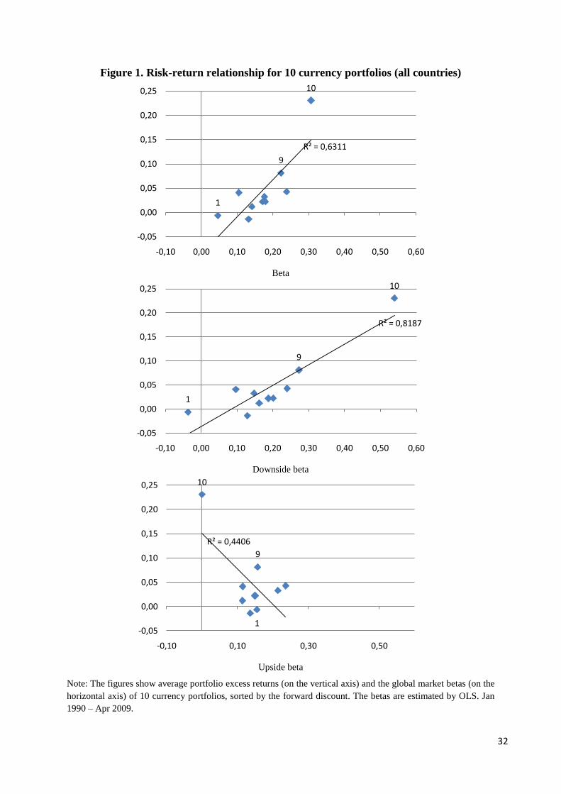
32

Figure 1. Risk-return relationship for 10 currency portfolios (all countries)

Beta

Downside beta

Upside beta

Note: The figures show average portfolio excess returns (on the vertical axis) and the global market betas (on the

horizontal axis) of 10 currency portfolios, sorted by the forward discount. The betas are estimated by OLS. Jan

1990 – Apr 2009.

1

9

10

R² = 0,6311

-0,05

0,00

0,05

0,10

0,15

0,20

0,25

-0,10 0,00 0,10 0,20 0,30 0,40 0,50 0,60

1

9

10

R² = 0,8187

-0,05

0,00

0,05

0,10

0,15

0,20

0,25

-0,10 0,00 0,10 0,20 0,30 0,40 0,50 0,60

1

9

10

R² = 0,4406

-0,05

0,00

0,05

0,10

0,15

0,20

0,25

-0,10 0,10 0,30 0,50

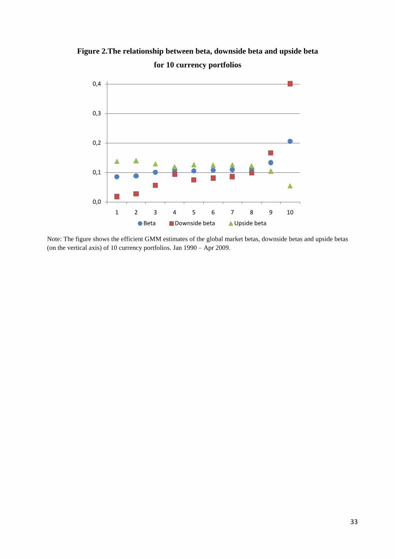
33

Figure 2.The relationship between beta, downside beta and upside beta

for 10 currency portfolios

Note: The figure shows the efficient GMM estimates of the global market betas, downside betas and upside betas

(on the vertical axis) of 10 currency portfolios. Jan 1990 – Apr 2009.

0,0

0,1

0,2

0,3

0,4

1 2 3 4 5 6 7 8 9 10

Beta Downside beta Upside beta

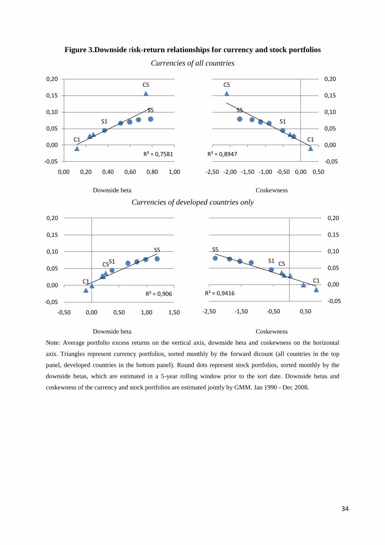
34

Figure 3.Downside risk-return relationships for currency and stock portfolios

Currencies of all countries

Downside beta

Coskewness

Currencies of developed countries only

Downside beta Coskewness

Note: Average portfolio excess returns on the vertical axis, downside beta and coskewness on the horizontal

axis. Triangles represent currency portfolios, sorted monthly by the forward dicount (all countries in the top

panel, developed countries in the bottom panel). Round dots represent stock portfolios, sorted monthly by the

downside betas, which are estimated in a 5-year rolling window prior to the sort date. Downside betas and

coskewness of the currency and stock portfolios are estimated jointly by GMM. Jan 1990 - Dec 2008.

C1

C5

S1

S5

R² = 0,7581-0,05

0,00

0,05

0,10

0,15

0,20

0,00 0,20 0,40 0,60 0,80 1,00

C1

C5

S1

S5

R² = 0,8947-0,05

0,00

0,05

0,10

0,15

0,20

-2,50 -2,00 -1,50 -1,00 -0,50 0,00 0,50

C1

C5S1

S5

R² = 0,906

-0,05

0,00

0,05

0,10

0,15

0,20

-0,50 0,00 0,50 1,00 1,50

C1

C5S1

S5

R² = 0,9416-0,05

0,00

0,05

0,10

0,15

0,20

-2,50 -1,50 -0,50 0,50

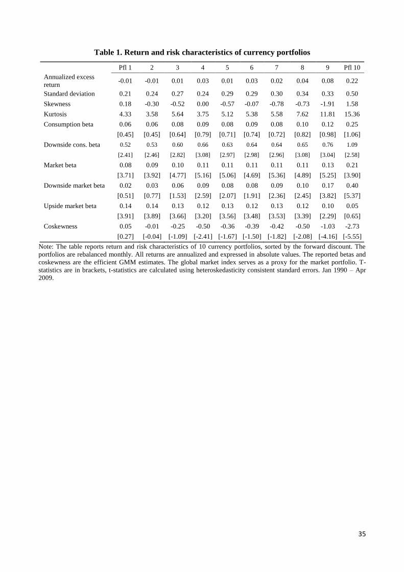
35

Table 1. Return and risk characteristics of currency portfolios

Pfl 1 2 3 4 5 6 7 8 9 Pfl 10

Annualized excess

return -0.01 -0.01 0.01 0.03 0.01 0.03 0.02 0.04 0.08 0.22

Standard deviation 0.21 0.24 0.27 0.24 0.29 0.29 0.30 0.34 0.33 0.50

Skewness 0.18 -0.30 -0.52 0.00 -0.57 -0.07 -0.78 -0.73 -1.91 1.58

Kurtosis 4.33 3.58 5.64 3.75 5.12 5.38 5.58 7.62 11.81 15.36

Consumption beta 0.06 0.06 0.08 0.09 0.08 0.09 0.08 0.10 0.12 0.25

[0.45] [0.45] [0.64] [0.79] [0.71] [0.74] [0.72] [0.82] [0.98] [1.06]

Downside cons. beta 0.52 0.53 0.60 0.66 0.63 0.64 0.64 0.65 0.76 1.09

[2.41] [2.46] [2.82] [3.08] [2.97] [2.98] [2.96] [3.08] [3.04] [2.58]

Market beta 0.08 0.09 0.10 0.11 0.11 0.11 0.11 0.11 0.13 0.21

[3.71] [3.92] [4.77] [5.16] [5.06] [4.69] [5.36] [4.89] [5.25] [3.90]

Downside market beta 0.02 0.03 0.06 0.09 0.08 0.08 0.09 0.10 0.17 0.40

[0.51] [0.77] [1.53] [2.59] [2.07] [1.91] [2.36] [2.45] [3.82] [5.37]

Upside market beta 0.14 0.14 0.13 0.12 0.13 0.12 0.13 0.12 0.10 0.05

[3.91] [3.89] [3.66] [3.20] [3.56] [3.48] [3.53] [3.39] [2.29] [0.65]

Coskewness 0.05 -0.01 -0.25 -0.50 -0.36 -0.39 -0.42 -0.50 -1.03 -2.73

[0.27] [-0.04] [-1.09] [-2.41] [-1.67] [-1.50] [-1.82] [-2.08] [-4.16] [-5.55]

Note: The table reports return and risk characteristics of 10 currency portfolios, sorted by the forward discount. The

portfolios are rebalanced monthly. All returns are annualized and expressed in absolute values. The reported betas and

coskewness are the efficient GMM estimates. The global market index serves as a proxy for the market portfolio. T-

statistics are in brackets, t-statistics are calculated using heteroskedasticity consistent standard errors. Jan 1990 – Apr

2009.

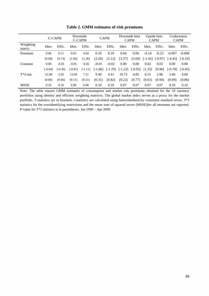
36

Table 2. GMM estimates of risk premiums

C-CAPM

Downside

C-CAPM CAPM

Downside beta

CAPM

Upside beta

CAPM

Coskewness

CAPM

Weighting

matrix Iden. Effic. Iden. Effic. Iden. Effic. Iden. Effic. Iden. Effic. Iden. Effic.

Premium 0.06 0.11 0.03 0.04 0.10 0.19 0.04 0.06 -0.14 -0.23 -0.007 -0.008

[0.08] [0.74] [1.06] [1.36] [2.20] [2.12] [3.57] [5.69] [-1.45] [-0.97] [-4.45] [-6.19]

Constant 0.00 -0.01 -0.01 -0.02 -0.01 -0.02 0.00 0.00 0.02 0.03 0.00 0.00

[-0.04] [-0.36] [-0.81] [-1.11] [-1.86] [-1.70] [-1.23] [-0.95] [1.35] [0.96] [-0.78] [-0.45]

T*J-stat 25.98 5.92 13.06 7.21 9.40 4.41 10.72 4.85 6.31 2.96 5.66 4.00

(0.00) (0.66) (0.11) (0.51) (0.31) (0.82) (0.22) (0.77) (0.61) (0.94) (0.69) (0.86)

MSSE 0.10 0.10 0.08 0.08 0.10 0.10 0.07 0.07 0.07 0.07 0.10 0.10

Note: The table reports GMM estimates of consumption and market risk premiums obtained for the 10 currency

portfolios using identity and efficient weighting matrices. The global market index serves as a proxy for the market

portfolio. T-statistics are in brackets, t-statistics are calculated using heteroskedasticity consistent standard errors. T*J

statistics for the overidentifying restrictions and the mean sum of squared errors (MSSE)for all moments are reported.

P-value for T*J statistics is in parentheses. Jan 1990 – Apr 2009.

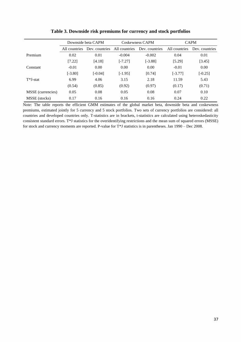
37

Table 3. Downside risk premiums for currency and stock portfolios

Downside beta CAPM Coskewness CAPM CAPM

All countries Dev. countries All countries Dev. countries All countries Dev. countries

Premium 0.02 0.01 -0.004 -0.002 0.04 0.01

[7.22] [4.18] [-7.27] [-3.88] [5.29] [3.45]

Constant -0.01 0.00 0.00 0.00 -0.01 0.00

[-3.80] [-0.04] [-1.95] [0.74] [-3.77] [-0.25]

T*J-stat 6.99 4.06 3.15 2.18 11.59 5.43

(0.54) (0.85) (0.92) (0.97) (0.17) (0.71)

MSSE (currencies) 0.05 0.08 0.05 0.08 0.07 0.10

MSSE (stocks) 0.17 0.16 0.16 0.16 0.24 0.22

Note: The table reports the efficient GMM estimates of the global market beta, downside beta and coskewness

premiums, estimated jointly for 5 currency and 5 stock portfolios. Two sets of currency portfolios are considered: all

countries and developed countries only. T-statistics are in brackets, t-statistics are calculated using heteroskedasticity

consistent standard errors. T*J statistics for the overidentifying restrictions and the mean sum of squared errors (MSSE)

for stock and currency moments are reported. P-value for T*J statistics is in parentheses. Jan 1990 – Dec 2008.

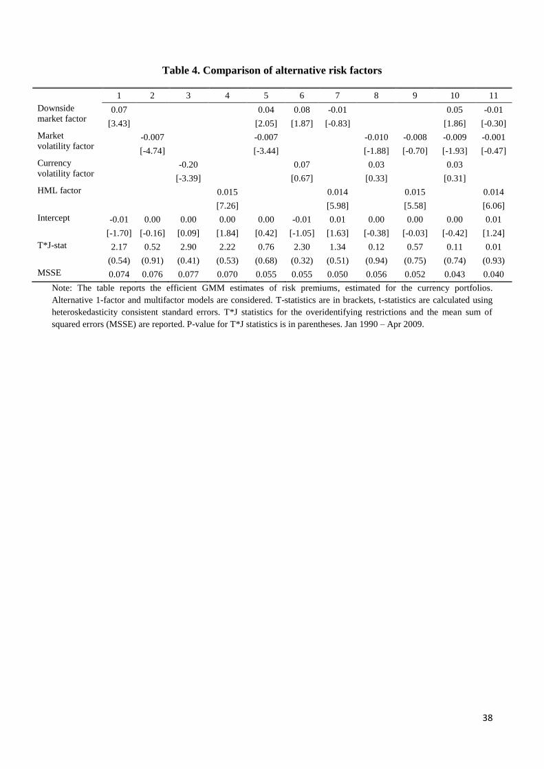
38

Table 4. Comparison of alternative risk factors

1 2 3 4 5 6 7 8 9 10 11

Downside

market factor 0.07

0.04 0.08 -0.01

0.05 -0.01

[3.43]

[2.05] [1.87] [-0.83]

[1.86] [-0.30]

Market

volatility factor -0.007

-0.007

-0.010 -0.008 -0.009 -0.001

[-4.74]

[-3.44]

[-1.88] [-0.70] [-1.93] [-0.47]

Currency

volatility factor -0.20

0.07

0.03

0.03

[-3.39]

[0.67]

[0.33]

[0.31]

HML factor

0.015

0.014

0.015

0.014

[7.26]

[5.98]

[5.58]

[6.06]

Intercept -0.01 0.00 0.00 0.00 0.00 -0.01 0.01 0.00 0.00 0.00 0.01

[-1.70] [-0.16] [0.09] [1.84] [0.42] [-1.05] [1.63] [-0.38] [-0.03] [-0.42] [1.24]

T*J-stat 2.17 0.52 2.90 2.22 0.76 2.30 1.34 0.12 0.57 0.11 0.01

(0.54) (0.91) (0.41) (0.53) (0.68) (0.32) (0.51) (0.94) (0.75) (0.74) (0.93)

MSSE 0.074 0.076 0.077 0.070 0.055 0.055 0.050 0.056 0.052 0.043 0.040

Note: The table reports the efficient GMM estimates of risk premiums, estimated for the currency portfolios.

Alternative 1-factor and multifactor models are considered. T-statistics are in brackets, t-statistics are calculated using

heteroskedasticity consistent standard errors. T*J statistics for the overidentifying restrictions and the mean sum of

squared errors (MSSE) are reported. P-value for T*J statistics is in parentheses. Jan 1990 – Apr 2009.

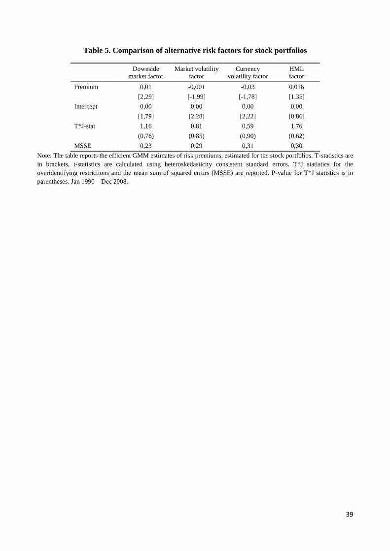
39

Table 5. Comparison of alternative risk factors for stock portfolios

Downside

market factor

Market volatility

factor

Currency

volatility factor

HML

factor

Premium 0,01 -0,001 -0,03 0,016

[2,29] [-1,99] [-1,78] [1,35]

Intercept 0,00 0,00 0,00 0,00

[1,79] [2,28] [2,22] [0,86]

T*J-stat 1,16 0,81 0,59 1,76

(0,76) (0,85) (0,90) (0,62)

MSSE 0,23 0,29 0,31 0,30

Note: The table reports the efficient GMM estimates of risk premiums, estimated for the stock portfolios. T-statistics are

in brackets, t-statistics are calculated using heteroskedasticity consistent standard errors. T*J statistics for the

overidentifying restrictions and the mean sum of squared errors (MSSE) are reported. P-value for T*J statistics is in

parentheses. Jan 1990 – Dec 2008.

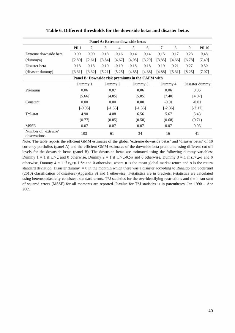
40

Table 6. Different thresholds for the downside betas and disaster betas

Panel A: Extreme downside betas

Pfl 1 2 3 4 5 6 7 8 9 Pfl 10

Extreme downside beta 0,09 0,09 0,13 0,16 0,14 0,14 0,15 0,17 0,23 0,48

(dummy4) [2,89] [2,61] [3,84] [4,67] [4,05] [3,29] [3,85] [4,66] [6,78] [7,49]

Disaster beta 0.13 0.13 0.19 0.19 0.18 0.18 0.19 0.21 0.27 0.50

(disaster dummy) [3.31] [3.32] [5.21] [5.25] [4.85] [4.38] [4.88] [5.31] [8.25] [7.07]

Panel B: Downside risk premiums in the CAPM with

Dummy 1 Dummy 2 Dummy 3 Dummy 4 Disaster dummy

Premium 0.06 0.07 0.06 0.06 0.06

[5.66] [4.85] [5.85] [7.40] [4.07]

Constant 0.00 0.00 0.00 -0.01 -0.01

[-0.95] [-1.55] [-1.36] [-2.86] [-2.17]

T*J-stat 4.90 4.08 6.56 5.67 5.48

(0.77) (0.85) (0.58) (0.68) (0.71)

MSSE 0.07 0.07 0.07 0.07 0.06

Number of 'extreme'

observations 103 61 34 16 41

Note: The table reports the efficient GMM estimates of the global „extreme downside betas‟ and „disaster betas‟ of 10

currency portfolios (panel A) and the efficient GMM estimates of the downside beta premiums using different cut-off

levels for the downside betas (panel B). The downside betas are estimated using the following dummy variables:

Dummy 1 = 1 if rm> and 0 otherwise, Dummy 2 = 1 if rm> -0.5σ and 0 otherwise, Dummy 3 = 1 if rm> -σ and 0

otherwise, Dummy 4 = 1 if rm> -1.5σ and 0 otherwise, where is the mean global market return and σ is the return

standard deviation; Disaster dummy = 0 in the monthin which there was a disaster according to Ranaldo and Soderlind

(2010) classification of disasters (Appendix 3) and 1 otherwise. T-statistics are in brackets, t-statistics are calculated

using heteroskedasticity consistent standard errors. T*J statistics for the overidentifying restrictions and the mean sum

of squared errors (MSSE) for all moments are reported. P-value for T*J statistics is in parentheses. Jan 1990 – Apr

2009.

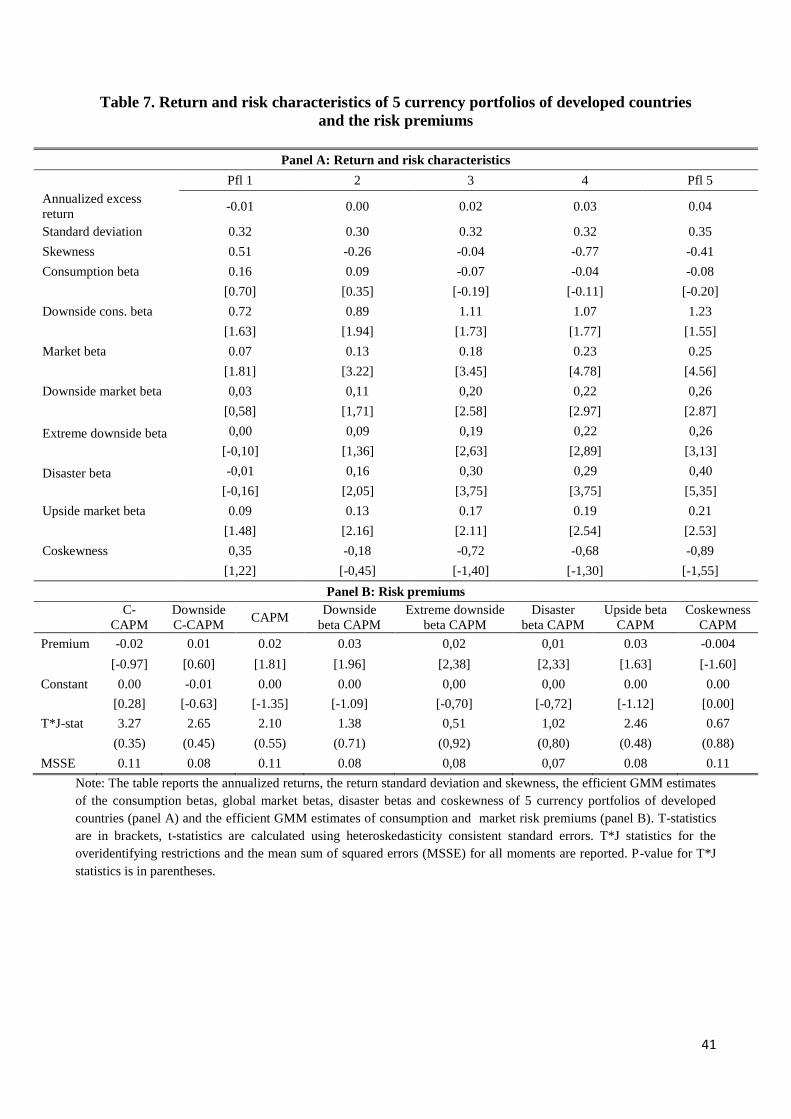
41

Table 7. Return and risk characteristics of 5 currency portfolios of developed countries

and the risk premiums

Panel A: Return and risk characteristics

Pfl 1 2 3 4 Pfl 5

Annualized excess

return -0.01 0.00 0.02 0.03 0.04

Standard deviation 0.32 0.30 0.32 0.32 0.35

Skewness 0.51 -0.26 -0.04 -0.77 -0.41

Consumption beta 0.16 0.09 -0.07 -0.04 -0.08

[0.70] [0.35] [-0.19] [-0.11] [-0.20]

Downside cons. beta 0.72 0.89 1.11 1.07 1.23

[1.63] [1.94] [1.73] [1.77] [1.55]

Market beta 0.07 0.13 0.18 0.23 0.25

[1.81] [3.22] [3.45] [4.78] [4.56]

Downside market beta 0,03 0,11 0,20 0,22 0,26

[0,58] [1,71] [2.58] [2.97] [2.87]

Extreme downside beta 0,00 0,09 0,19 0,22 0,26

[-0,10] [1,36] [2,63] [2,89] [3,13]

Disaster beta -0,01 0,16 0,30 0,29 0,40

[-0,16] [2,05] [3,75] [3,75] [5,35]

Upside market beta 0.09 0.13 0.17 0.19 0.21

[1.48] [2.16] [2.11] [2.54] [2.53]

Coskewness 0,35 -0,18 -0,72 -0,68 -0,89

[1,22] [-0,45] [-1,40] [-1,30] [-1,55]

Panel B: Risk premiums

C-

CAPM

Downside

C-CAPM CAPM

Downside

beta CAPM

Extreme downside

beta CAPM

Disaster

beta CAPM

Upside beta

CAPM

Coskewness

CAPM

Premium -0.02 0.01 0.02 0.03 0,02 0,01 0.03 -0.004

[-0.97] [0.60] [1.81] [1.96] [2,38] [2,33] [1.63] [-1.60]

Constant 0.00 -0.01 0.00 0.00 0,00 0,00 0.00 0.00

[0.28] [-0.63] [-1.35] [-1.09] [-0,70] [-0,72] [-1.12] [0.00]

T*J-stat 3.27 2.65 2.10 1.38 0,51 1,02 2.46 0.67

(0.35) (0.45) (0.55) (0.71) (0,92) (0,80) (0.48) (0.88)

MSSE 0.11 0.08 0.11 0.08 0,08 0,07 0.08 0.11

Note: The table reports the annualized returns, the return standard deviation and skewness, the efficient GMM estimates

of the consumption betas, global market betas, disaster betas and coskewness of 5 currency portfolios of developed

countries (panel A) and the efficient GMM estimates of consumption and market risk premiums (panel B). T-statistics

are in brackets, t-statistics are calculated using heteroskedasticity consistent standard errors. T*J statistics for the

overidentifying restrictions and the mean sum of squared errors (MSSE) for all moments are reported. P-value for T*J

statistics is in parentheses.

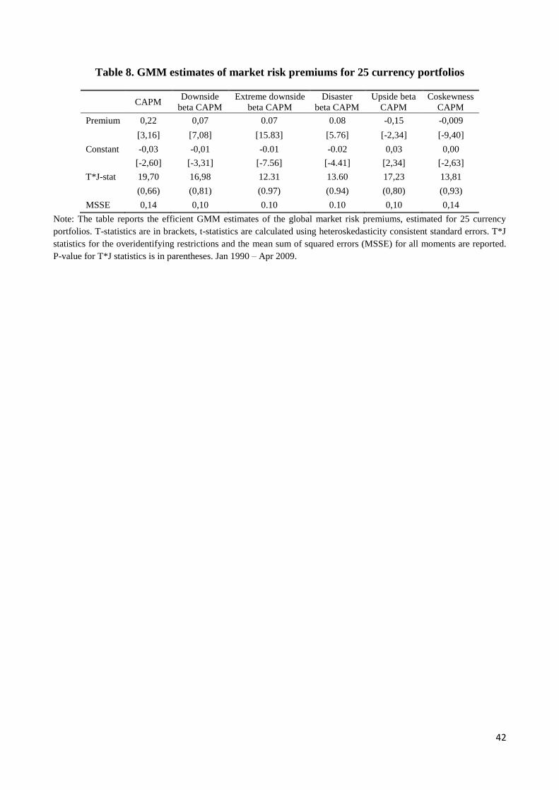
42

Table 8. GMM estimates of market risk premiums for 25 currency portfolios

CAPM

Downside

beta CAPM

Extreme downside

beta CAPM

Disaster

beta CAPM

Upside beta

CAPM

Coskewness

CAPM

Premium 0,22 0,07 0.07 0.08 -0,15 -0,009

[3,16] [7,08] [15.83] [5.76] [-2,34] [-9,40]

Constant -0,03 -0,01 -0.01 -0.02 0,03 0,00

[-2,60] [-3,31] [-7.56] [-4.41] [2,34] [-2,63]

T*J-stat 19,70 16,98 12.31 13.60 17,23 13,81

(0,66) (0,81) (0.97) (0.94) (0,80) (0,93)

MSSE 0,14 0,10 0.10 0.10 0,10 0,14

Note: The table reports the efficient GMM estimates of the global market risk premiums, estimated for 25 currency

portfolios. T-statistics are in brackets, t-statistics are calculated using heteroskedasticity consistent standard errors. T*J

statistics for the overidentifying restrictions and the mean sum of squared errors (MSSE) for all moments are reported.

P-value for T*J statistics is in parentheses. Jan 1990 – Apr 2009.

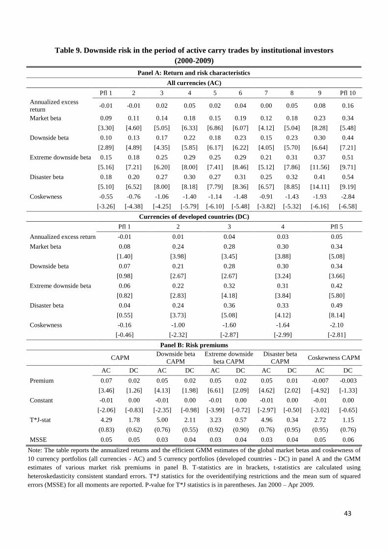
43

Table 9. Downside risk in the period of active carry trades by institutional investors

(2000-2009)

Panel A: Return and risk characteristics

All currencies (AC)

Pfl 1 2 3 4 5 6 7 8 9 Pfl 10

Annualized excess

return -0.01 -0.01 0.02 0.05 0.02 0.04 0.00 0.05 0.08 0.16

Market beta 0.09 0.11 0.14 0.18 0.15 0.19 0.12 0.18 0.23 0.34

[3.30] [4.60] [5.05] [6.33] [6.86] [6.07] [4.12] [5.04] [8.28] [5.48]

Downside beta 0.10 0.13 0.17 0.22 0.18 0.23 0.15 0.23 0.30 0.44

[2.89] [4.89] [4.35] [5.85] [6.17] [6.22] [4.05] [5.70] [6.64] [7.21]

Extreme downside beta 0.15 0.18 0.25 0.29 0.25 0.29 0.21 0.31 0.37 0.51

[5.16] [7.21] [6.20] [8.00] [7.41] [8.46] [5.12] [7.86] [11.56] [9.71]

Disaster beta 0.18 0.20 0.27 0.30 0.27 0.31 0.25 0.32 0.41 0.54

[5.10] [6.52] [8.00] [8.18] [7.79] [8.36] [6.57] [8.85] [14.11] [9.19]

Coskewness -0.55 -0.76 -1.06 -1.40 -1.14 -1.48 -0.91 -1.43 -1.93 -2.84

[-3.26] [-4.38] [-4.25] [-5.79] [-6.10] [-5.48] [-3.82] [-5.32] [-6.16] [-6.58]

Currencies of developed countries (DC)

Pfl 1 2 3 4 Pfl 5

Annualized excess return -0.01 0.01 0.04 0.03 0.05

Market beta 0.08 0.24 0.28 0.30 0.34

[1.40] [3.98] [3.45] [3.88] [5.08]

Downside beta 0.07 0.21 0.28 0.30 0.34

[0.98] [2.67] [2.67] [3.24] [3.66]

Extreme downside beta 0.06 0.22 0.32 0.31 0.42

[0.82] [2.83] [4.18] [3.84] [5.80]

Disaster beta 0.04 0.24 0.36 0.33 0.49

[0.55] [3.73] [5.08] [4.12] [8.14]

Coskewness -0.16 -1.00 -1.60 -1.64 -2.10

[-0.46] [-2.32] [-2.87] [-2.99] [-2.81]

Panel B: Risk premiums

CAPM

Downside beta

CAPM

Extreme downside

beta CAPM

Disaster beta

CAPM Coskewness CAPM

AC DC AC DC AC DC AC DC AC DC

Premium 0.07 0.02 0.05 0.02 0.05 0.02 0.05 0.01 -0.007 -0.003

[3.46] [1.26] [4.13] [1.98] [6.61] [2.09] [4.62] [2.02] [-4.92] [-1.33]

Constant -0.01 0.00 -0.01 0.00 -0.01 0.00 -0.01 0.00 -0.01 0.00

[-2.06] [-0.83] [-2.35] [-0.98] [-3.99] [-0.72] [-2.97] [-0.50] [-3.02] [-0.65]

T*J-stat 4.29 1.78 5.00 2.11 3.23 0.57 4.96 0.34 2.72 1.15

(0.83) (0.62) (0.76) (0.55) (0.92) (0.90) (0.76) (0.95) (0.95) (0.76)

MSSE 0.05 0.05 0.03 0.04 0.03 0.04 0.03 0.04 0.05 0.06

Note: The table reports the annualized returns and the efficient GMM estimates of the global market betas and coskewness of

10 currency portfolios (all currencies - AC) and 5 currency portfolios (developed countries - DC) in panel A and the GMM

estimates of various market risk premiums in panel B. T-statistics are in brackets, t-statistics are calculated using

heteroskedasticity consistent standard errors. T*J statistics for the overidentifying restrictions and the mean sum of squared

errors (MSSE) for all moments are reported. P-value for T*J statistics is in parentheses. Jan 2000 – Apr 2009.

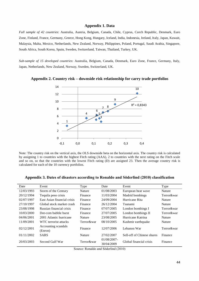
44

Appendix 1. Data

Full sample of 42 countries: Australia, Austria, Belgium, Canada, Chile, Cyprus, Czech Republic, Denmark, Euro

Zone, Finland, France, Germany, Greece, Hong Kong, Hungary, Iceland, India, Indonesia, Ireland, Italy, Japan, Kuwait,

Malaysia, Malta, Mexico, Netherlands, New Zealand, Norway, Philippines, Poland, Portugal, Saudi Arabia, Singapore,

South Africa, South Korea, Spain, Sweden, Switzerland, Taiwan, Thailand, Turkey, UK.

Sub-sample of 15 developed countries: Australia, Belgium, Canada, Denmark, Euro Zone, France, Germany, Italy,

Japan, Netherlands, New Zealand, Norway, Sweden, Switzerland, UK.

Appendix 2. Country risk – downside risk relationship for carry trade portfolios

Note: The country risk on the vertical axis, the OLS downside beta on the horizontal axis. The country risk is calculated

by assigning 1 to countries with the highest Fitch rating (AAA), 2 to countries with the next rating on the Fitch scale

and so on, so that the countries with the lowest Fitch rating (D) are assigned 23. Then the average country risk is

calculated for each of the 10 currency portfolios.

Appendix 3. Dates of disasters according to Ronaldo and Söderlind (2010) classification

Date Event Type Date Event Type

12/03/1993 Storm of the Century Nature 01/08/2003 European heat wave Nature

20/12/1994 Tequila peso crisis Finance 11/03/2004 Madrid bombings Terror&war

02/07/1997 East Asian financial crisis Finance 24/09/2004 Hurricane Rita Nature

27/10/1997 Global stock market crash Finance 26/12/2004 Tsunami Nature

23/08/1998 Russian financial crisis Finance 07/07/2005 London bombings I Terror&war

10/03/2000 Dot-com bubble burst Finance 27/07/2005 London bombings II Terror&war

04/06/2001 2001 Atlantic hurricane Nature 23/08/2005 Hurricane Katrina Nature

11/09/2001 WTC terrorist attacks Terror&war 08/10/2005 Kashmir earthquake Nature

02/12/2001 Accounting scandals

(Enron) Finance 12/07/2006 Lebanon War Terror&war

01/11/2002 SARS Nature 27/02/2007 Sell-off of Chinese shares Finance

20/03/2003 Second Gulf War Terror&war 01/08/2007-

30/04/2009 Global financial crisis Finance

Source: Ronaldo and Söderlind (2010)

1

23

4 56

7 8

9

10

R² = 0,8343

0

2

4

6

8

10

12

14

-0,1 0,0 0,1 0,2 0,3 0,4