Embed Size (px)
Citation preview

DOWNSLOPE PIPELINE WALKING AND SOIL
VARIABLES
by
Adriano Condez Gondarém Castelo
B.E., MSc
A thesis submitted for the degree of
Doctor of Philosophy
at
The University of Western Australia
Centre for Offshore Foundation Systems
School of Civil and Resource Engineering
February 2020


Downslope pipeline walking and soil variables
i
ABSTRACT
Operational loading cycles of startup and shutdown phases have a major impact on a
pipeline’s behaviour over its lifetime. Some pipelines are long enough to generate a soil
reaction that anchors the pipeline in an overall fixed position on the seabed. For these
pipelines, the loading cycles generate symmetric expansion and contraction at the ends
of the pipeline caused by variations in temperature and pressure. A related phenomenon
named “pipeline walking” causes the pipeline to migrate globally in one direction.
Pipeline walking occurs whenever a pipeline extension is shorter than necessary thereby
leading to axial instability associated with an asymmetry between expansions and
contractions over the total length of the pipeline.
Current analytical methodologies used during early design stages of pipelines, provide
results to estimate the pipe walking susceptibility and the corresponding walking pattern
for rigid-plastic soils. However, the basic rigid-plastic soil assumption of these
methodologies leads to an overestimation of the walking response. As a result, protracted
and costly finite element analyses need to be performed, so that a more realistic walking
prediction may be achieved. Further, while it is common practice in the industry to
assume an elastic-perfectly-plastic soil reaction, field and laboratory tests show that soils
may behave very differently from elastic-perfectly-plastic. To account for these
differences, the industry assumes two different conditions of elastic-perfectly-plasticity:
the “Stiff Fit” and the “Soft Fit”. They represent the lower and upper bounds to create a
case envelope of soil resistance. Thus, there is a demand to improve the accuracy, the
cost- and time-effectiveness of the current analyses.
This thesis starts by assuming an elastic-perfectly-plastic idealization for elastic-plastic
soils followed by the analysis of the non-linear elastic-plastic soil models. For these soil
considerations, a number of innovative analytical solutions for pipeline walking are
proposed and benchmarked against finite element analyses. The reasons for the difference
between the new and the current solutions are explored and corrections to the current
analytical methodologies are proposed to make them applicable to all types of soil
conditions (elastic-plastic soils with a linear or a non-linear behaviour). These corrections
reduce time and financial demands of a project since finite element analyses are no longer
required.

Downslope pipeline walking and soil variables
ii
However, field and laboratory tests show that some soils may present a breakout peak
resistance. For instance, for clayey soils the peak breakout resistance depends largely on
the over consolidation ratio and for sandy soils it depends on dilatancy. The loading
process, potentially even including intermittent consolidation cycles, may also influence
peak resistance occurrence. These particularities of loading processes complicate the soil
reaction models considered by this research.
In this thesis, breakout peak resistance was initially idealized as a tri-linear peaky spring
to account for peak resistance. Two different cases were investigated: (1) peak breakout
resistance for the loading and unloading steps; and (2) peak breakout for just the loading
step. These two cases represent the variability that soils may impose on pipe-soil
interaction behaviours, when breakout resistance must be accounted for. Based on our
elastic-plastic modelling, finite element models were used as a general platform to
numerically determine how to correct the rigid-plastic analytical solution to account for
the breakout resistance. The corrections were then used to account for tri-linear soil
behaviours to accurately calculate the walking rates.
A more detailed approach was then taken to consider the non-linearities of a peak
breakout resistance soil model thereby further improving the peaky soil model and the
interpretation of the impact of the non-linearities of peaky soils. The numerical results
were used to establish the necessary corrections for the walking rate calculations resulting
in a valid correction – similar to the non-linear elastic-plastic – of the original rigid-plastic
solution.
The influence of different slope geometries was investigated, given the fact that real
pipelines traverse routes that often slope continuously down, but at a varying pace.
Numerical results were used to show that an average slope throughout the entire route
can be assumed so that the previous findings could still be successfully applied for these
bathymetric conditions.
Overall, this thesis presents a significant improvement to commonly applied methods for
estimating pipeline walking rates. Using the proposed solutions, realistic walking patterns
are now quickly and easily obtained. The methodology presented can optimize any
pipeline project by reducing turn-around time, costs and increasing the accuracy of the
walking patterns estimated.

February 2020
February 2020
February 2020
February 2020
February 2020
February 2020

February 2020
February 2020
February 2020
February 2020
February 2020
Thesis Declaration
v
I, Adriano Condez Gondarém Castelo, certify that:
This thesis has been substantially accomplished during enrolment in this degree.
This thesis does not contain material which has been submitted for the award of any other
degree or diploma in my name, in any university or other tertiary institution.
In the future, no part of this thesis will be used in a submission in my name, for any other
degree or diploma in any university or other tertiary institution without the prior approval
of The University of Western Australia and where applicable, any partner institution
responsible for the joint-award of this degree.
This thesis does not contain any material previously published or written by another
person, except where due reference has been made in the text and, where relevant, in the
Authorship Declaration that follows.
This thesis does not violate or infringe any copyright, trademark, patent, or other rights
whatsoever of any person.
This thesis contains published work and/or work prepared for publication, some of which
has been co-authored.
Signature:
Date: February 2020
Downslope pipeline walking and soil variables
vi
ACKNOWLEDGEMENTS
First of all, I would like to express my gratitude to my PhD supervisors Dave, Yinghui,
Mark and Christophe, without your help this thesis would never be achieved.
I also thank my MSc supervisor and evaluator, Nelson and Gilberto, for all the help
provided during the PhD application process.
Thanks also to the friends from UWA for touch rugby, soccer and uncountable hours of
lunch, discussions (technical or not) and fun. Special mentions to Colm, Simon, Dunja
and Wensong – all from Room 2.63; along with Liang, Susie, Dana, Lisa, Yuxia, Behnaz,
Charlie, Andrew, Diego, Fillippo, Jiayue, João, Maria, Manu, Mark, Max, Mike, Mirko,
Nicole, Pauline, Raffa, Serena, Tao, Youkou and Yusuke.
I couldn’t fail to mention some people, who we met in Perth; and made life here a lot
easier: Alex & Mickle, CC, Daniel & Rô, Edu & Monique, Flávio & Marcinha, Francisco
& Olivia, Gabriel & Andrea, Laerte & Luana, Leo & Lu, Luiz & Raquel, Marcelo &
Aline, Murray & Patrica, Shelley and Tiago & Sara.
Finally, my deepest thanks to my parents, Paulo and Guiomar, for giving me the best start
in life one could ever ask for and your constant support.
This thesis is dedicated to an incredible woman, whom I have the pleasure and honour
to refer to as “my dearest and beloved wife”, Lorena.
This research was supported by an Australian Government Research Training Program (RTP) Scholarship.
“Dans un axiome que vous appliquez à vos sciences: il n'y a pas d'effet sans cause.
Cherchez la cause de tout ce qui n'est pas l'oeuvre de l'homme, et votre raison vous
répondra.”
⸻ Allan Kardec, Le Livre Des Esprits

Downslope pipeline walking and soil variables
vii
TABLE OF CONTENTS
Abstract ............................................................................................................................ i
Publications arising from this thesis ............................................................................ iii
Acknowledgements ........................................................................................................ vi
Table of contents ........................................................................................................... vii
List of tables ................................................................................................................. xiii
List of figures ................................................................................................................ xv
Nomenclature ............................................................................................................... xix
Chapter 1. Introduction ................................................................................................. 1
1.1 Pipeline walking ................................................................................................ 2
1.2 Thesis objectives ............................................................................................... 5
1.3 Thesis organisation ............................................................................................ 5
Chapter 2. Literature review ......................................................................................... 8
2.1 Pipelines and pipeline walking .......................................................................... 9
2.2 Current analytical method ............................................................................... 11
2.2.1 Mathematical Shortcuts .................................................................. 13
2.3 Axial Pipe-soil Interaction ............................................................................... 13
2.3.1 Axial pipe-soil interaction models ................................................. 15
2.4 Possible Mitigation Strategies ......................................................................... 18
2.5 Final Remarks .................................................................................................. 22
Chapter 3. Simple solutions for downslope pipeline walking on elastic-perfectly-
plastic soils ..................................................................................................................... 31
3.1 Abstract ........................................................................................................... 32
3.2 Introduction ..................................................................................................... 32
3.3 Background to pipeline walking ...................................................................... 34
3.4 Problem Definition .......................................................................................... 35
3.5 Rigid-plastic analytical solutions .................................................................... 36
3.6 Finite element analyses methodology ............................................................. 37
3.7 Finite element analyses comparison with rigid-plastic solution ..................... 39
3.8 Xab for elastic-perfectly-plastic soil ................................................................. 40
3.9 ΔSS for elastic-perfectly-plastic soil ................................................................ 40
3.9.1 δx Boundary Conditions .................................................................. 41
3.9.2 Effective Axial Force Boundary Conditions .................................. 41
3.9.3 Effective Axial Force Pipe Differential Equation .......................... 42
3.9.4 ΔSS Revision ................................................................................... 43
Downslope pipeline walking and soil variables
viii
3.10 Walking rate for elastic-perfectly-plastic soil ................................................. 43
3.11 Finite element analyses parametric study ....................................................... 44
3.12 Conclusions & final remarks ........................................................................... 46
Chapter 4. Solving downslope pipeline walking on non-linear elastic-plastic
soils ................................................................................................................................. 60
4.1 Abstract ........................................................................................................... 61
4.2 Introduction ..................................................................................................... 61
4.3 Background to pipeline walking ..................................................................... 62
4.3.1 Downslope mechanism .................................................................. 62
4.3.2 Pipe-soil response ........................................................................... 63
4.4 Problem definition ........................................................................................... 63
4.5 Elastic-perfectly-plastic solution for pipeline walking ................................... 65
4.6 Finite element methodology ............................................................................ 66
4.6.1 Introduction .................................................................................... 66
4.6.2 Dual-spring pipe-soil interaction model ......................................... 67
4.6.3 Multi-spring pipe-soil interaction model ........................................ 67
4.6.4 Loads .............................................................................................. 67
4.7 Finite element analysis results and comparison with elastic-perfectly-
plastic solution ................................................................................................ 67
4.8 New analytical solutions for non-linear elastic-plastic soil ............................ 68
4.8.1 Displacement profile ...................................................................... 68
4.8.2 Displacement boundary conditions ................................................ 69
4.8.3 Effective axial force boundary conditions ..................................... 69
4.8.4 Effective axial force profile ............................................................ 71
4.8.5 Analytical solution for walking rate ............................................... 72
4.9 Revised solution for the distance between stationary points for non-linear
elastic-plastic soil - XAB,NLEP ............................................................................ 73
4.10 Revised solution for walking rate for non-linear elastic-plastic soil –
WRNLEP............................................................................................................. 73
4.11 Equivalent mobilisation distance – δmobEQ ...................................................... 74
4.12 Finite element analyses parametric study for dual-spring strategy ................. 74
4.12.1 Equivalent mobilisation distance – δmobEQ ..................................... 75
4.12.2 Distance between stationary points for non-linear elastic-plastic
soil – Xab,NLEP ................................................................................................... 77

Downslope pipeline walking and soil variables
ix
4.12.3 Walking rate for non-linear elastic-plastic soil – WRNLEP .............. 78
4.13 Finite element analysis for multi-spring strategy ............................................ 78
4.13.1 Rigid-plastic preliminary calculations ............................................ 78
4.13.2 Non-linear elastic-plastic calculations ............................................ 78
Equivalent mobilisation distance – δmobEQ ....................................................... 78
Distance between stationary points for non-linear elastic-plastic soil –
Xab,NLEP 78
Walking rate for non-linear elastic-plastic soil – WRNLEP ............................... 79
4.13.3 Non-linear elastic-plastic finite element model results .................. 79
Distance between stationary points from finite element analysis – Xab,FEM .... 79
Walking rate from finite element analysis – WRFEM ....................................... 79
4.14 Conclusions & final remarks ........................................................................... 79
Chapter 5. Solutions for downslope pipeline walking on peaky tri-linear soils ..... 93
5.1 Abstract ........................................................................................................... 94
5.2 Introduction ..................................................................................................... 94
5.3 Background to pipeline walking ...................................................................... 96
5.3.1 Downslope mechanism ................................................................... 96
5.3.2 Pipe-soil response ........................................................................... 96
5.4 Problem definition ........................................................................................... 96
5.5 Elastic-perfectly-plastic solution for pipeline walking ................................... 98
5.6 Finite element methodology ............................................................................ 99
5.6.1 Peaky tri-linear pipe-soil interaction models ................................ 100
5.6.2 Loads ............................................................................................ 100
5.7 Finite element analysis results and comparison with rigid-plastic solution .. 100
5.8 Revised analytical solution for the distance between stationary points for
peaky tri-linear soils – Xab,3L .......................................................................... 101
5.9 Revised analytical solution for the walking rate for peaky tri-linear soils –
WR3L .............................................................................................................. 102
5.10 Ideal mobilisation distance - δmob’ ................................................................. 102
5.11 Finite element analyses parametric study for peaky tri-linear pipe-soil
interaction ...................................................................................................... 104
5.11.1 Ideal mobilisation distance - δmob’ ................................................ 104
5.11.2 Distance between stationary points for peaky tri-linear soil –
Xab,3L 104

Downslope pipeline walking and soil variables
x
5.11.3 Walking rate for peaky tri-linear soil – WR3L .............................. 105
5.12 Observations about the effective axial force variation over the distance
between stationary points for peaky tri-linear soils – ΔSS,3L ......................... 106
5.13 Conclusions & final remarks ......................................................................... 106
Chapter 6. Solving downslope pipeline walking on non-linear soil with brittle
peak strength and strain softening ........................................................................... 117
6.1 Abstract ......................................................................................................... 118
6.2 Introduction ................................................................................................... 119
6.2.1 Pipeline walking mechanisms ...................................................... 119
6.2.2 Walking phenomenon on a rigid-plastic basis ............................. 120
6.2.3 Walking consequences ................................................................. 121
6.2.4 Axial pipe-soil non-linearity ........................................................ 122
6.3 Problem definition ......................................................................................... 123
6.3.1 General Properties of Study-Case ................................................ 123
6.3.2 Variations in axial pipe-soil response .......................................... 124
6.4 Rigid-plastic analytical solutions .................................................................. 125
6.4.1 Calculations .................................................................................. 125
6.4.2 Rigid-plastic analytical results ..................................................... 125
6.5 NLBPSS FEM solution ................................................................................. 126
6.5.1 FEM architecture .......................................................................... 126
Loads 126
Pipe-soil interaction representation ............................................................... 127
6.5.2 FEM results .................................................................................. 128
FEM results ................................................................................................... 128
6.5.3 Axial displacement ....................................................................... 129
FEM results crosscheck ................................................................................. 129
FEM results summary ................................................................................... 130
6.6 Results comparison ....................................................................................... 131
6.6.1 Effective axial force ..................................................................... 131
6.6.2 Stationary points ........................................................................... 131
6.6.3 Axial displacements & walking rates ........................................... 132
6.7 Equivalent mobilisation distance .................................................................. 133
Downslope pipeline walking and soil variables
xi
6.7.1 Back evaluation ............................................................................ 133
6.8 Conclusions & final remarks ......................................................................... 134
Chapter 7. Gravity-driven pipeline walking on variable slopes ............................ 147
7.1 Abstract ......................................................................................................... 148
7.2 Introduction ................................................................................................... 148
7.3 Background to pipeline walking .................................................................... 149
7.3.1 Downslope walking mechanisms ................................................. 149
7.3.2 Route topography ......................................................................... 150
7.4 Problem definition ......................................................................................... 150
7.5 Elastic-perfectly-plastic solution for pipeline walking on single slope ........ 152
7.6 Finite element methodology .......................................................................... 152
7.7 Range of parametric studies .......................................................................... 154
7.7.1 Dual slope – convex ..................................................................... 154
7.7.2 Dual slope – concave .................................................................... 155
7.7.3 Triple slope – flat-slope-flat ......................................................... 157
7.7.4 Triple slope – flat-slope-flat ......................................................... 158
7.8 Finite element model results .......................................................................... 159
7.9 Conclusions & final remarks ......................................................................... 164
Chapter 8. Concluding remarks ................................................................................ 170
8.1 Principal findings and contributions .............................................................. 171
8.1.1 Pipe-soil interaction models ......................................................... 171
Elastic-perfectly-plastic ................................................................................. 171
Non-linear elastic-plastic ............................................................................... 172
Tri-linear with a peak .................................................................................... 172
Non-linear with a peak .................................................................................. 172
General notes ................................................................................................. 173
8.1.2 Variable slopes ............................................................................. 173
8.1.3 A new assessment of downslope pipeline walking ...................... 173
8.2 Further research recommendations ............................................................... 175

Downslope pipeline walking and soil variables
xii
REFERENCES ........................................................................................................... 176
Appendix A ................................................................................................................. 180
Appendix B .................................................................................................................. 184
Appendix C ................................................................................................................. 185
Appendix D ................................................................................................................. 190

Downslope pipeline walking and soil variables
xiii
LIST OF TABLES
Table 2.1: Summary of possible walking mitigation strategies (Rong et al., 2009).
................................................................................................................... 21
Table 2.2: Summary of causes of uncertainty and thesis chapters. ................................ 24
Table 3.1: Preliminary example properties. ................................................................... 36
Table 3.2: Rigid-plastic analytical results. ..................................................................... 37
Table 3.3: Elastic-perfectly-plastic FEA results. ............................................................ 39
Table 3.4: Pipeline zoning. ............................................................................................. 41
Table 3.5: EAF boundary conditions.............................................................................. 42
Table 3.6: FEA parametric variables. ............................................................................. 44
Table 4.1: Preliminary example properties – Dual-Spring UEL. ................................... 64
Table 4.2: Preliminary example properties – Multi-Spring UEL. .................................. 65
Table 4.3: Elastic-perfectly-plastic analytical results. .................................................... 66
Table 4.4: Elastic-perfectly-plastic general results. ....................................................... 68
Table 4.5: Pipeline zoning. ............................................................................................. 69
Table 4.6: Mobilisation distance, δmob, combination cases. ........................................... 75
Table 4.7: Resultant equivalent mobilisation distance, δmobEQ. ...................................... 76
Table 4.8: Resultant non-walking mobilisation distance, δnull. ...................................... 77
Table 5.1: General properties. ........................................................................................ 97
Table 5.2: Case properties. ............................................................................................. 97
Table 5.3: Tri-linear finite element analysis results for soil case ii. ............................. 101
Table 5.4: Rigid-plastic calculation results. ................................................................. 101
Table 5.5: Analytical results. ........................................................................................ 103
Table 5.6: Tri-linear finite element analyses results. ................................................... 105
Table 6.1: Pipeline properties. ...................................................................................... 123
Table 6.2: Axial pipe-soil interaction model parameters. ............................................ 124
Table 6.3: Analytical results. ........................................................................................ 125
Table 6.4: Key aspects from rigid-plastic solution. ...................................................... 126
Table 6.5: EAF notable results. .................................................................................... 129

Downslope pipeline walking and soil variables
xiv
Table 6.6: δx notable results. ........................................................................................ 129
Table 6.7: FEM crosscheck results. ............................................................................. 130
Table 6.8: FEM summary results. ................................................................................ 130
Table 6.9: EAF comparison. ........................................................................................ 131
Table 6.10: SPs comparison. ........................................................................................ 131
Table 6.11: Walking rates for different soil approaches. ............................................. 132
Table 6.12: Equations (6.9) and (6.11) results. ............................................................ 133
Table 7.1: Environmental properties ............................................................................ 151
Table 7.2: Operational properties ................................................................................. 151
Table 7.3: Physical pipeline properties ........................................................................ 151
Table 7.4: Dual slope convex model properties ........................................................... 154
Table 7.5: Dual slope concave model properties ......................................................... 156
Table 7.6: Triple slope flat-slope-flat model properties ............................................... 157
Table 7.7: Triple slope slope-flat-slope model properties ............................................ 158
Table 7.8: Dual slope – Convex model results ............................................................. 159
Table 7.9: Dual slope – Concave model results ........................................................... 160
Table 7.10: Triple slope flat-slope-flat model results .................................................. 162
Table 7.11: Triple slope slope-flat-slope model results ............................................... 163
Table 8.1: Preliminary example properties. ................................................................. 173
Table B.1: Base cases comparison ............................................................................... 184
Table C.1: Mesh sensitivity checks .............................................................................. 185
Table D.1: Lateral buckling check ............................................................................... 190

Downslope pipeline walking and soil variables
xv
LIST OF FIGURES
Figure 1.1: Axial stability design stairs ............................................................................ 7
Figure 2.1: Example for field architecture of infield pipelines and production
infrastructure units from White (2011). ..................................................... 25
Figure 2.2: Effective axial force diagrams for start-up and shutdown loading
phases. ........................................................................................................ 25
Figure 2.3: Axial displacement diagrams for start-up and shutdown loading
phases. ........................................................................................................ 26
Figure 2.4: Rigid-plastic soil behaviour. ........................................................................ 27
Figure 2.5: Axial friction curves (no peak) – adapted from White et al. (2011)............ 27
Figure 2.6: Axial friction curve (peak in one direction) – adapted from Hill and
Jacob (2008). .............................................................................................. 28
Figure 2.7: Different soil resistance behaviours. ............................................................ 28
Figure 2.8: Walking mitigation devices from Frazer et al. (2007). ................................ 29
Figure 2.9: Pipeline walking accumulated displacement from Frankenmolen et al.
(2017). ........................................................................................................ 29
Figure 2.10: Pipe-clamping mattress from Frankenmolen et al. (2017). ....................... 30
Figure 2.11: Post pipe-clamping mattresses installation walking monitoring from
Frankenmolen et al. (2017). ....................................................................... 30
Figure 3.1: EAF diagrams for SUp and SDown phases. ................................................ 47
Figure 3.2: δx diagrams for SUp and SDown phases. ..................................................... 48
Figure 3.3: Rigid-plastic & elastic-plastic soil responses. ............................................. 49
Figure 3.4: Finite element model sketch. ....................................................................... 49
Figure 3.5: EAF plot (zoom). ......................................................................................... 50
Figure 3.6: δx plot for Stiff Fit (zoom). .......................................................................... 51
Figure 3.7: δx plot for Soft Fit (zoom). ........................................................................... 51
Figure 3.8: x coordinate for the stationary points. .......................................................... 52
Figure 3.9: Xab,EP results against δmob. ............................................................................ 52
Figure 3.10: Schematic plot accounting physical boundaries. ....................................... 53
Figure 3.11: Schematic EAF plot with the partial areas highlight. ................................ 53
Figure 3.12: Xab,EP results for 1° slope. .......................................................................... 54
Downslope pipeline walking and soil variables
xvi
Figure 3.13: Xab,EP results – numerical & calculated for 1° slope. ................................. 54
Figure 3.14: Xab,EP results for 2° slope. .......................................................................... 55
Figure 3.15: Xab,EP results – numerical & calculated for 2° slope. ................................. 55
Figure 3.16: Xab,EP results for 3° slope. .......................................................................... 56
Figure 3.17: Xab,EP results – numerical & calculated for 3° slope. ................................. 56
Figure 3.18: WREP results for 1° slope. .......................................................................... 57
Figure 3.19: WREP results – numerical & calculated for 1° slope. ................................. 57
Figure 3.20: WREP results for 2° slope. .......................................................................... 58
Figure 3.21: WREP results – numerical & calculated for 2° slope. ................................. 58
Figure 3.22: WREP results for 3° slope. .......................................................................... 59
Figure 3.23: WREP results – numerical & calculated for 3° slope. ................................. 59
Figure 4.1: Effective axial force diagrams for start-up and shutdown phases. .............. 81
Figure 4.2: Axial displacement diagrams for start-up and shutdown phases. ................ 82
Figure 4.3: Rigid-plastic, elastic-perfectly-plastic and non-linear elastic-plastic
soil responses. ............................................................................................ 83
Figure 4.4: Dual-spring finite element analysis methodology (as per values from
Table 4.1). .................................................................................................. 83
Figure 4.5: Multi-spring finite element analysis methodology (as per values from
Table 4.2). .................................................................................................. 84
Figure 4.6: Effective axial force for non-linear elastic-plastic soil – dual-spring
(zoom). ....................................................................................................... 85
Figure 4.7: Axial displacement for non-linear elastic-plastic soil – dual-spring
(zoom). ....................................................................................................... 86
Figure 4.8: x coordinate for the stationary points – dual-spring. ................................... 86
Figure 4.9: Effective axial force for non-linear elastic-plastic soil – multi-spring
(zoom). ....................................................................................................... 87
Figure 4.10: Axial displacement for non-linear elastic-plastic soil – multi-spring
(zoom). ....................................................................................................... 88
Figure 4.11: x coordinate for the stationary points – multi-spring. ................................ 88
Figure 4.12: Schematic plot accounting physical boundaries. ....................................... 89
Figure 4.13: Schematic plot accounting physical boundaries. ....................................... 89
Figure 4.14: Mobilisation distance, δmob, combination spectrum. .................................. 90

Downslope pipeline walking and soil variables
xvii
Figure 4.15: Non-linear elastic correction results. ......................................................... 90
Figure 4.16: Walking rate from finite element models, WRFEM, results for selected
cases. .......................................................................................................... 91
Figure 4.17: Distance between stationary points results. ............................................... 91
Figure 4.18: Walking rate results. .................................................................................. 92
Figure 5.1: Effective axial force diagrams for start-up and shutdown phases. ............ 108
Figure 5.2: Axial displacement diagrams for start-up and shutdown phases. .............. 109
Figure 5.3: Tri-linear soil responses. ............................................................................ 110
Figure 5.4: Tri-linear soil responses for cyclic movements. ........................................ 111
Figure 5.5: Effective axial force for tri-linear strategy case ii – EqualPeaks
(Zoom). .................................................................................................... 112
Figure 5.6: Axial displacement for tri-linear strategy case ii – EqualPeaks (Zoom).
................................................................................................................. 113
Figure 5.7: Effective axial force for tri-linear strategy case ii – NoSUpPeak
(Zoom). .................................................................................................... 114
Figure 5.8: Axial displacement for tri-linear strategy case ii– NoSUpPeak (Zoom).
................................................................................................................. 115
Figure 5.9: Tri-linear correction results........................................................................ 115
Figure 5.10: Distance between stationary points results. ............................................. 116
Figure 5.11: Walking rate results. ................................................................................ 116
Figure 6.1: EAF diagram and sketch of acting loads. .................................................. 135
Figure 6.2: EAF diagrams for start-up and shutdown. ................................................. 135
Figure 6.3: Axial displacement – 1st cycle. .................................................................. 136
Figure 6.4: Axial displacement – further cycles. .......................................................... 137
Figure 6.5: Axial PSI non-linear approach. .................................................................. 138
Figure 6.6: Axial PSI boundaries. ................................................................................ 139
Figure 6.7: Analytical EAF plot. .................................................................................. 139
Figure 6.8: Schematic behaviours plot. ........................................................................ 140
Figure 6.9: Subroutine flowchart. ................................................................................. 141
Figure 6.10: EAF results for Cases A and B. ............................................................... 142
Figure 6.11: EAF zoom for Cases A and B. ................................................................. 143

Downslope pipeline walking and soil variables
xviii
Figure 6.12: δx results for Cases A and B..................................................................... 144
Figure 6.13: δx zoom for Cases A and B. ..................................................................... 145
Figure 6.14: Obtaining δmobEQ – for Cases A and B. .................................................... 146
Figure 7.1: Effective axial force diagrams ................................................................... 166
Figure 7.2: Axial displacement diagrams ..................................................................... 166
Figure 7.3: Finite element model sketch ...................................................................... 167
Figure 7.4: User element behavior ............................................................................... 167
Figure 7.5: Dual slope general shapes .......................................................................... 168
Figure 7.6: Triple slope general shapes ........................................................................ 168
Figure 7.7: Walking rate results ................................................................................... 169

Downslope pipeline walking and soil variables
xix
NOMENCLATURE
The nomenclature has been selected in an effort to retain consistency with previously
published work.

Downslope pipeline walking and soil variables
xx
Latin Symbols
A pipeline steel cross-sectional area
AUnload-Reload unload-reload area
A1 parabola 1 factor A
A2 parabola 2 factor A
A3 parabola 3 factor A
B1 parabola 1 factor B
B2 parabola 2 factor B
B3 parabola 3 factor B
CorrEP elastic correction
CorrNLEP non-linear elastic correction
Corr3L tri-linear correction
C1 parabola 1 factor C
C2 parabola 2 factor C
C3 parabola 3 factor C
D water depth
E steel Young’s modulus
FA mobilised axial resistance force
FElastic elastic limit force
FP soil peak elastic force
FR soil residual plastic force
F1 soil spring limiting force 1
F2 soil spring limiting force 2
F3 soil spring limiting force 3
F4 soil spring limiting force 4
FS1 plastic force for spring S1
FS2 plastic force for spring S2
Downslope pipeline walking and soil variables
xxi
FS3 plastic force for spring S3
FS4 plastic force for spring S4
FS5 plastic force for spring S5
FTotal total spring plastic force
FS_m final mobilised axial soil spring force
FS_Ref initial mobilised axial soil spring force
KSoil tangential soil stiffness
K1 differential equation constant 1
K2 differential equation constant 2
L pipeline physical length
LTotal total pipeline physical length
L1 partial pipeline physical length 1
L2 partial pipeline physical length 2
L3 partial pipeline physical length 3
OD cross section steel outside diameter
R2 coefficient of determination
s distance to stationary point
t steel wall thickness
UA_m final node axial position
UA_Ref initial node axial position
W pipeline operational submerged weight
Wcomp pipeline operational submerged weight longitudinal component
WR walking rate
x longitudinal axis along pipe length
x12 physical boundary between Z1 and Z2
x23 physical boundary between Z2 and Z3
x34 physical boundary between Z3 and Z4

Downslope pipeline walking and soil variables
xxii
x45 physical boundary between Z4 and Z5
x56 physical boundary between Z5 and Z6
Xab distance between stationary points

Downslope pipeline walking and soil variables
xxiii
Greek Symbols
steel thermal expansion coefficient
β seabed slope angle
βave average seabed slope angle
β1 partial seabed slope angle 1
β2 partial seabed slope angle 2
β3 partial seabed slope angle 3
δ general displacement
mob mobilisation distance
mobEQ equivalent mobilisation distance
mobP peak elastic force mobilisation distance
mobR residual plastic force mobilisation distance
mobS1 mobilisation distance for spring S1
mobS2 mobilisation distance for spring S2
mobS3 mobilisation distance for spring S3
mobS4 mobilisation distance for spring S4
mobS5 mobilisation distance for spring S5
mobSoft mobilisation distance for “Soft Fit”
mobStiff mobilisation distance for “Soft Fit”
mob’ ideal mobilisation distance
null non-walking mobilisation distance
x axial displacement
δ1 limiting displacement 1
δ2 limiting displacement 2
δ3 limiting displacement 3
δ4 limiting displacement 4

Downslope pipeline walking and soil variables
xxiv
FR variation in residual friction
p pressure variation
P change in fully constrained force
Ss change in effective axial force over Xab
T temperature variation
Mech mechanical strain
Thermal thermal strain
Total total strain
soil axial residual friction coefficient
WZ1 soil resistance in Z1
WZ2 soil resistance in Z2
WZ3 soil resistance in Z3
WZ4 soil resistance in Z4
WZ5 soil resistance in Z5
WZ6 soil resistance in Z6
steel Poisson coefficient
exponential factor
Downslope pipeline walking and soil variables
xxv
Abbreviations
Calc calculated
CAPEX capital expenditure
COFS Centre for Offshore Foundation Systems
EP elastic-perfectly-plastic
EAF effective axial force
EPCorr elastic-perfectly-plastic correction
EqualPeaks soil behaviour with equal peaks for both loading phases – start-up
and shutdown.
FE finite element
FEA finite element analysis
FEM finite element model
FxD soil force-displacement curve
HPHT high pressure high temperature
JIP joint industry project
KP kilometre post
NLEP non-linear elastic-plastic
NLBPSS non-linear soil with brittle peak strength and strength softening
NoSUpPeak soil behaviour with no peak for start-up phases, while peaky for
shutdown phases
OPEX operating expenses
PCM pipe-clamping mattress
PSI pipe-soil interaction
PW pipeline walking
RP rigid-plastic
SCR steel catenary riser
SDown shutdown phase
Downslope pipeline walking and soil variables
xxvi
SUp start-up phase
SP stationary point
S1 partial spring S1
S2 partial spring S2
S3 partial spring S3
S4 partial spring S4
S5 partial spring S5
UEL user-element
UWA The University of Western Australia
VAS virtual anchor section
WR walking rate
Z1 pipeline zone 1
Z2 pipeline zone 2
Z3 pipeline zone 3
Z4 pipeline zone 4
Z5 pipeline zone 5
Z6 pipeline zone 6
3L tri-linear peaky soil idealization


Introduction
1
CHAPTER 1. INTRODUCTION
Chapter context: This chapter introduces the research topic of this thesis highlighting
its importance and impact for the engineering community. The objectives and
organisation of this thesis are also presented.
Chapter 1
2
1.1 PIPELINE WALKING
Hydrocarbon fluids need to be transported from their natural reservoirs to consumption
centres. There are two main methods of transporting hydrocarbons: in a ship’s tank or in
a pipeline. Although pipelines require a large capital investment and are a fixed asset,
they present advantages when compared to voyages of cargo, which demand high
operating costs and represent a higher risk to the environment (Palmer and King, 2008).
Offshore pipelines became important as the hydrocarbon sources become more difficult
to be reached. Pipelines became an essential facility for the oil and gas industry when the
North Sea area arose as a major hydrocarbons producer in the 1970s (Kyriakides and
Corona, 2007).
As exemplified by Kumar and Mcshane (2009); Palmer and Croasdale (2012); Leckie et
al. (2016); and Azevedo et al. (2018), some hydrocarbon resources could not be feasible
for production without the presence of pipelines in areas such as the Gulf of Mexico, the
Arctic, the Australian Northwest Shelf, and the Brazilian Pre-Salt.
Given the relevance of pipelines, it is understandable that pipeline stability is a major
issue for both pipeline and geotechnical engineering (through the pipe-soil interaction).
Pipeline stability is determined by hydrodynamic loads and the effects of expansion and
contraction triggered by the high pressure/ high temperature operational conditions.
These two characteristics constitute the major focus of geotechnical design for pipelines.
Unlike other types of engineered solutions for foundations, pipelines can support some
movements across the seabed without exceeding a limit state (exceptions must be made
for regions where pipelines are connected to other structures). Hence, pipelines may be
designed to not be stable at the position at which they were installed; but in these cases,
it is necessary to predict and assess all movements that may occur during a pipeline
operational lifetime.
These movements may occur in the vertical plane, as a progressive burial or exposure of
the pipeline, and in the horizontal plane, as lateral or axial sliding (White and Cathie,
2011). These movements may be combined in many different ways, that have been
studied (isolated and combined) by many authors – (Palmer and Baldry, 1974; Tornes et
al., 2000; Carr et al., 2003; Bruton et al., 2008, 2009; Randolph and White, 2008; Sinclair
et al., 2009; Watson et al., 2010; Bruton et al., 2010; Bruton and Carr, 2011b, 2011a;
Watson et al., 2011; White et al., 2011; Smith and White, 2014).

Introduction
3
The movements may be related to different phenomena, which mainly are: lateral
buckling, upheaval buckling and pipeline walking. Other phenomena examples are: route
curve pull-out and lateral ratcheting. These phenomena are called global buckling
(DNVGL, 2018), which together form the general pipeline response to internal pressure
and temperature cycles. This thesis addresses the axial sliding movement that relates to
the pipeline walking phenomenon that can affect pipelines under thermal and pressure
cyclical loads.
Tornes et al. (2000), based on Konuk (1998), developed the concept of “axial creeping”,
which is the phenomenon of the net axial displacement of pipelines induced by thermal
and pressure increments and decrements associated with the operational cycles, after
monitoring operating offshore pipelines in the North Sea when this anomaly was first
observed. Later, the “axial creeping” phenomenon was renamed “pipeline walking”,
which is induced by the same principles as axial creeping, but with a broader
understanding of its causes, effects and consequences (Carr et al., 2003).
Different causes of pipeline walking have been understood (Bruton et al., 2010); but now
it is important to better understand the relationship between the pipeline subjected to
walking and the seabed soil.
Figure 1.1 illustrates the current industry methodology for pipeline walking assessment.
It shows a staircase with multiple steps representing the different steps of the design
procedure applied to the assessment of pipeline walking. The first step represents the
input data set; a step where basic information should be gathered to support the
assessments. General information such as pipeline route and fluid characterization are
considered to be given. The second step highlights the analytical solutions. The analytical
assessments are to be performed according to Carr et al. (2003). If the pipeline is not
proved stable, the third step of the methodology should be applied: simple Finite Element
Model (FEM). Simple finite element models account for simplified route geometry,
simplified flow assurance, and pipe-soil interaction models; which represent more basic
data. Even though simplified data deliver basic pipeline walking results, these results are
reliable and robust for the level of simplifications applied to the assessment. In case the
pipeline could not be proved stable by the simple finite element analyses, the fourth step
of the methodology is applied: a detailed finite element model. These models require
detailed data such as flow assurance, detailed tri-dimensional route geometry, realistic
pipe-soil interaction models and detailed pipeline geometry so that a design digital twin

Chapter 1
4
could be generated, and the assessment provides a final answer for the pipeline walking
evaluation. For cases that the detailed finite element analyses cannot prove the pipeline
stable, a mitigation design should be prepared. The mitigation design is the fifth step in
the axial stability design stairs. The mitigation is an engineered solution to prevent
pipeline walking from occurring and to eliminate any related issue to axial stability. The
next step is where all construction data come together to enable a finite element model
that should account for every construction detail in order to forecast the walking
behaviour. Finally, the last step of additional intervention is a safety net which allows
rectification in case discrepancies are found between operational surveys and as-built
forecast.
When results inform that mitigation is required, different types of apparatus have been
used to provide an additional resistance to axial displacement, which aims to cease
pipeline walking. Various anchoring structures, that provide the additional resistance,
have been used to moor different pipelines to their installation position on the seabed
(Rong et al., 2009; Carneiro and Murphy, 2011; Perinet and Simon, 2011). Regardless of
the method of choice, the methods proposed by these authors increase the axial resistance
available. However, they all consider some sort of intervention in the pipeline, which
increases costs and time requirements.
Thus, an evaluation of the previous design steps can be performed to assess potential
improvements that could assist to avoid the mitigation step. To do so, it is mandatory to
look for improvements in the previous models (analytical and computational) and how
they can be adjusted. Especially when the relationship between soil and pipeline (i.e.
pipe-soil interaction) is considered, which is the main source of uncertainty of this type
of assessment.
The traditional analytical solution considers an idealized pipe-soil interaction model
commonly called “rigid-plastic” (Carr et al., 2006). This idealization clearly opposes the
realistic pipe-soil interaction behaviour observed in various published sample tests
(White and Cathie, 2011; White et al., 2011, 2012; Hill et al., 2012). Therefore, this thesis
aims to extend the validity of analytical techniques by generating alternative solutions
that are shown to properly represent more complex and realistic soil conditions than the
idealized rigid-plastic interaction.
Introduction
5
By extending the validity of analytical solutions, this thesis also contributes to cheaper
and quicker engineering assessments because it sits in a lower step of the investment
staircase (Figure 1.1) when compared to other solutions (finite element analyses).
1.2 THESIS OBJECTIVES
This thesis’s goal is to extend the analytical solutions so that cost and time efficient
assessments could be done reliably. This thesis improves the quality of analytical and
numerical models for pipeline walking assessments by accounting for an extended range
of potential soil conceptualizations and also evaluates the impact of different slope
geometries on pipeline walking as many pipelines are deployed in such conditions
(Leckie et al., 2016).
To successfully improve our understanding of pipeline walking, the following
intermediate goals are defined: (i) establish a perfectly elastic-plastic soil spring and
investigate its influence on pipeline walking, (ii) develop a non-linear elastic-plastic soil
model and inspect its impact on walking pattern, (iii) elaborate and investigate the
consequences of the use of a tri-linear peaky soil on the walking rates, (iv) create a non-
linear peaky soil behaviour and understand its effect on the pipeline walking phenomenon
and (v) investigate the effects of different slope geometries on pipeline walking.
1.3 THESIS ORGANISATION
This thesis has 8 chapters, including the Introduction (Chapter 1), Literature Review
(Chapter 2) and the Conclusion (Chapter 8). Chapter 2 provides an extended literature
review covering concepts associated with pipeline walking and engineering topics
essential for the research presented in this thesis.
In Chapter 3, perfectly elastic-plastic soils are treated and their impact on pipeline
walking is explored, by establishing how such soil springs can be mimicked and by
investigating its influence on pipeline walking.
Chapter 4 considers a non-linear non-peaky behaviour (non-linear elastic-plastic soil
models). The non-linear elastic-plastic soil models are developed and their influence on
pipeline walking is inspected.
In Chapter 5, peaky linear soils are treated (peaky tri-linear); while Chapter 6 considers
a non-linear soil approach (non-linear peaky). In such chapters the soil models are created

Chapter 1
6
to mimic peaky soil behaviour and their impact on pipeline walking could be understood,
for the peaky tri-linear and non-linear peaky soil behaviours, respectively.
Chapter 7 investigates the impact variable slopes have on pipeline walking, regardless
the pipe-soil interaction model.
Chapter 8 concludes this thesis by covering the research findings generated in the
previous chapters and presenting some suggestions for future research.
Appendix A gives more details on the pile/ pipe equivalence as stated by Section 3.9
accordingly with Randolph (1977).
Appendix B helps a better understanding by providing a base case comparison in one
(cheat) sheet for all pipe-soil interaction models used in this thesis (Chapters 3, 4, 5, and
6).
Appendix C provides some additional information about finite element model details.
Appendix D provides the calculation check for lateral buckling for all models used in this
thesis (Chapters 3, 4, 5, 6 and 7). Although the coupled problem of walking and lateral
buckling is not the aim of this thesis, these calculations are provided here in order to show
that some cases studied are not susceptible to lateral buckling; whilst some other cases
are. Therefore, it can be understood that even illustration cases (i.e. cases that could suffer
lateral buckling) of the different soil characterization still have value for practical and
real situations. All cases (with or without lateral buckling susceptibility) follow through
the patterns established by this study.

Introduction
7
FIGURES
Figure 1.1: Axial stability design stairs

Chapter 2
8
CHAPTER 2. LITERATURE REVIEW
Chapter context: Pipeline walking is a complex and a relatively new phenomenon that
is yet not fully understood. This chapter reviews the relevant literature on pipeline
walking, including relevant information on supporting topics, such as offshore
geotechnics experimental investigations, numerical modelling and industry adopted
strategies/ mitigation measures, among others.

Literature review
9
2.1 PIPELINES AND PIPELINE WALKING
Since the 1970s, offshore pipelines became increasingly essential facilities for
hydrocarbon production (Kyriakides and Corona, 2007) and nowadays they are seen as
the arteries of offshore oil and gas production systems (Palmer and King, 2008).
For various reasons, certain hydrocarbon resources need a complex production network
as exemplified in Figure 2.1. Despite having many different parts and pieces of
infrastructure, this type of production network became very usual in areas such as the
Gulf of Mexico, Australasia, Offshore Brazil and West Africa (Jayson et al., 2008;
Carneiro and Castelo, 2011; Roberts et al., 2018). Such arrangements of production
network require short pipelines, typically in the vicinity of 2km (Carr et al., 2003; Carr
et al., 2006); while, export pipelines are significantly longer. For example, Solano et al.
(2014) and Charnaux et al. (2015) reported pipeline lengths of approximately 40km.
In 2000 (Tornes et al., 2000), unpredicted pipeline movements were noticed in a few
short infield pipelines in the North Sea – UK Sector. These movements occurred while
operating under high pressure and high temperature conditions and could potentially have
caused an environmental disaster. This phenomenon was named pipeline walking (Carr,
et al., 2003), and represents a major challenge to pipelines’ operations.
Pipeline walking consists of a global axial migration of the pipeline. This migration is a
progressive pattern of movements that accumulates over the operational design life of a
pipeline. The movements are induced by asymmetries in expansion and contraction
cycles due to start-up and shutdown loading stages.
Further, industry based research found more information on this engineering topic, which
established the foundation for following designs and applications (Bruton et al., 2010).
Four distinct mechanisms have been identified to date to incite pipeline walking:
1. Thermal transients along the line (Tornes et al., 2000);
2. Tension at the end of the flowline (Carr et al., 2003);
3. Seabed slopes along the pipeline route (Carr et al., 2006);
4. Multiphase fluid behaviour during restart operations (Bruton et al., 2010).
The tension at the end of the flowline causes the pipeline to walk towards the tensioned
end (Carr et al., 2003). For example, this tension might be created by a riser directly
connected to the pipeline. Direct connections are normally avoided by including some
infrastructure piece to the connection. In Figure 2.1 it can be seen that the pipeline system
Chapter 2
10
includes holdback suction anchors (near the spar platform) and the pipeline end
termination structures (near the floating production, storage and offloading, FPSO, unit).
Thermal transient is the mechanism originally reported by Tornes et al. (2000) and occurs
when the operational conditions imposed a variable temperature profile along the length
of the pipeline. Although this is a common issue in operating pipelines, in assessments
the temperature variation along the entire length could generally be approximated to the
steady state operational temperature variation.
The multiphase fluid behaviour during restart operations is related to not so trivial
operational conditions where gasses and liquids are conveyed together in the same
pipeline (Bruton et al., 2010). The problem arises when the pipeline is shutdown and the
fluids separate due to different individual densities. The separation creates a variation of
total weight along the line, which increases the chances of pipeline walking.
The seabed slopes mechanism generates a weight component along the longitudinal
pipeline axis thereby increasing the likelihood of the pipeline walking occurrence (Carr
et al., 2006). This weight component modifies the pipe-soil interaction behaviour in a
way that allows the pipeline to slip downhill. The seabed slopes mechanism is the most
commonly observed cause of pipeline walking, and as such it is the focus of the research
developed in this thesis.
Changes in temperature and pressure can lead to unexpected pipeline movements caused
by physical expansion and contraction. In start-up phases, increments in temperature and
pressure generate a pipeline axial expansion. Pipe-soil interaction resists this expansion,
resulting in effective compression of the pipeline. During shutdown phases, decrements
in temperature and pressure can cause physical contraction; inducing effective tension
due to the physical contraction of the pipeline.
For pipelines in which these cycles of compression and tension do not cancel each other,
pipeline walking may occur as a result of asymmetric effective axial force along the
pipeline. Each of the four mechanisms is capable of creating the referred unbalance in
axial displacements and the asymmetric pipeline effective axial force. Therefore, pipeline
walking appears because of the pipeline effective axial force asymmetry, causing unequal
pipeline displacements between cycles of start-up and shutdown loading phases.
Industry research (Carr et al., 2003) also highlights two categories of pipelines regarding
downslope pipeline walking:

Literature review
11
1. “Long” pipelines;
2. “Short” pipelines;
These categories are not exclusively related to the pipeline physical length because they
also involve pipe-soil interaction characteristics (e.g., friction factors and mobilisation
distances). As an example, the exact same pipeline may behave as “long” for a certain set
of pipe-soil interaction, while it may behave as “short” for another set of pipe-soil
interaction. The soil resistance would help determine conditions in which the pipeline
would behave as “long” or “short”.
For “long” pipelines, the soil provides resistance so that the effective compression build-
up occurs along a sufficient length to induce enough mechanical strain to fully
compensate for the thermo-mechanical expansion during the hot stages. For “short”
pipelines, the compression build-up, due to soil resistance, is not sufficient to fully
compensate for the expansion.
When “short” pipelines are located on a sloping seabed and are not anchored, cycles of
expansion and contraction may cause the pipelines to move with geometric asymmetries
between the start-up and shutdown phases. The sloping seabed generates a component of
weight to act parallel with the seabed in a downslope direction.
Even if pipeline walking may not present a serious structural issue to the pipeline itself,
it may result in several design challenges, including:
1. Overstressing of end connections (and in-line connections);
2. Loss of tension in a SCR;
3. Increased loading leading to lateral buckling;
4. Route instability (curve pull out);
5. Need for anchoring mitigation.
Therefore, pipeline walking must be avoided since its consequences may create
downtime and environmental risk, as pointed out by Tornes et al. (2000).
2.2 CURRENT ANALYTICAL METHOD
For the downslope mechanism of pipeline walking, the effective axial force plot
demonstrates the asymmetry, as referred in Section 2.1 and shown in Figure 2.2. This
asymmetry, which accounts for the weight component action, controls the offset distance
Xab, which is the distance between the virtual anchor sections as defined by Carr et al.
Chapter 2
12
(2003). Xab is also noticeable in the different profiles of axial displacement, δx, as shown
in Figure 2.3.
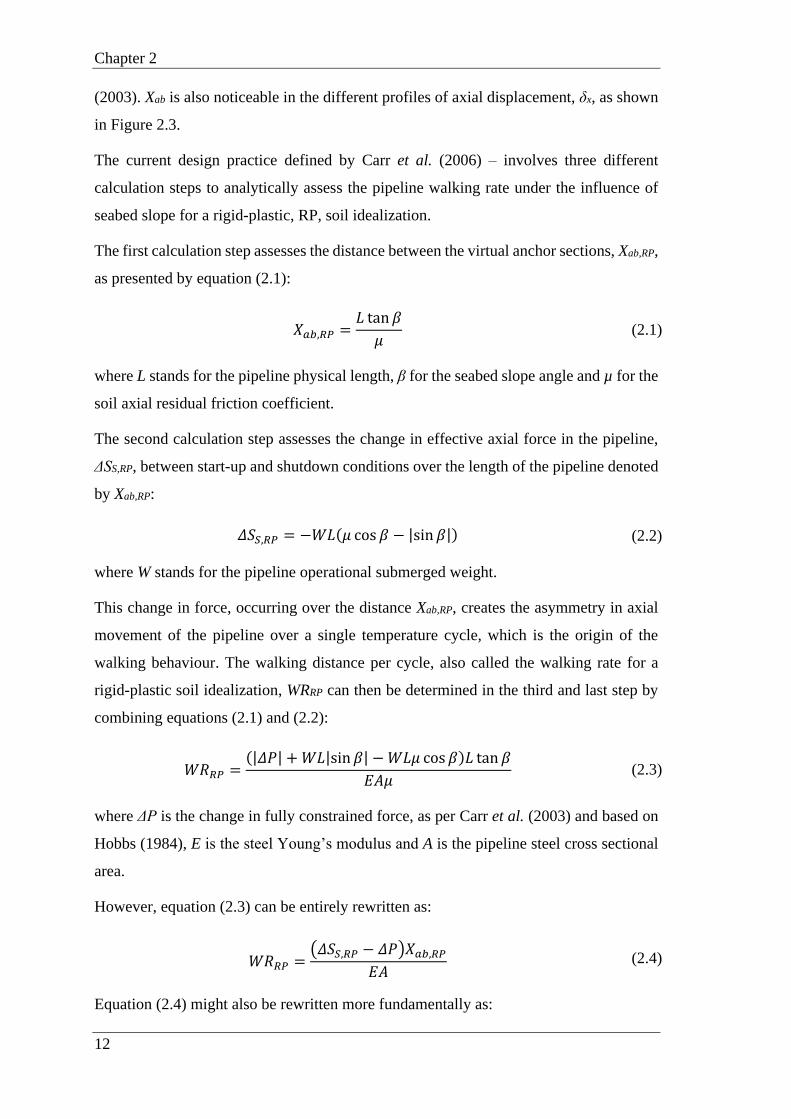
The current design practice defined by Carr et al. (2006) – involves three different
calculation steps to analytically assess the pipeline walking rate under the influence of
seabed slope for a rigid-plastic, RP, soil idealization.
The first calculation step assesses the distance between the virtual anchor sections, Xab,RP,
as presented by equation (2.1):
𝑋𝑎𝑏,𝑅𝑃 =𝐿 tan𝛽
𝜇 (2.1)
where L stands for the pipeline physical length, β for the seabed slope angle and µ for the
soil axial residual friction coefficient.
The second calculation step assesses the change in effective axial force in the pipeline,
ΔSS,RP, between start-up and shutdown conditions over the length of the pipeline denoted
by Xab,RP:
𝛥𝑆𝑆,𝑅𝑃 = −𝑊𝐿(𝜇 cos 𝛽 − |sin 𝛽|) (2.2)
where W stands for the pipeline operational submerged weight.
This change in force, occurring over the distance Xab,RP, creates the asymmetry in axial
movement of the pipeline over a single temperature cycle, which is the origin of the
walking behaviour. The walking distance per cycle, also called the walking rate for a
rigid-plastic soil idealization, WRRP can then be determined in the third and last step by
combining equations (2.1) and (2.2):
𝑊𝑅𝑅𝑃 =(|𝛥𝑃| +𝑊𝐿|sin 𝛽| −𝑊𝐿𝜇 cos 𝛽)𝐿 tan 𝛽
𝐸𝐴𝜇 (2.3)
where ΔP is the change in fully constrained force, as per Carr et al. (2003) and based on
Hobbs (1984), E is the steel Young’s modulus and A is the pipeline steel cross sectional
area.
However, equation (2.3) can be entirely rewritten as:
𝑊𝑅𝑅𝑃 =(𝛥𝑆𝑆,𝑅𝑃 − 𝛥𝑃)𝑋𝑎𝑏,𝑅𝑃
𝐸𝐴 (2.4)
Equation (2.4) might also be rewritten more fundamentally as:
Literature review
13
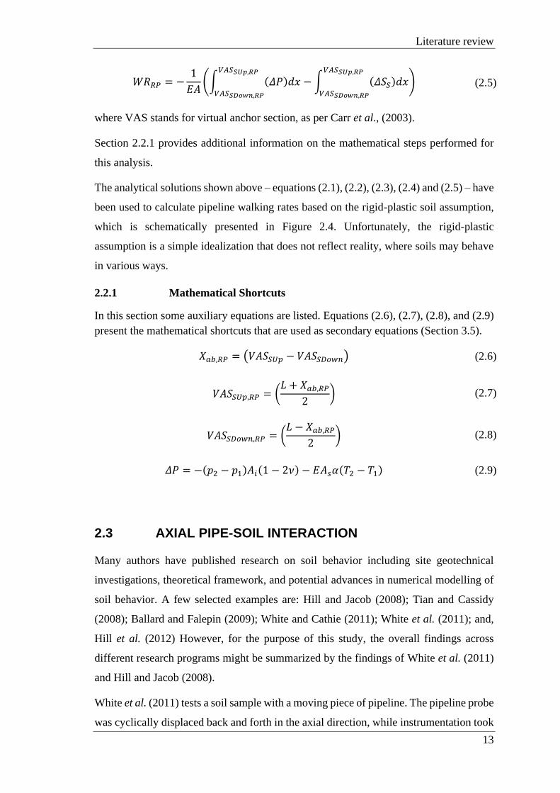
𝑊𝑅𝑅𝑃 = −1
𝐸𝐴(∫ (𝛥𝑃)𝑑𝑥
𝑉𝐴𝑆𝑆𝑈𝑝,𝑅𝑃
𝑉𝐴𝑆𝑆𝐷𝑜𝑤𝑛,𝑅𝑃
−∫ (𝛥𝑆𝑆)𝑑𝑥𝑉𝐴𝑆𝑆𝑈𝑝,𝑅𝑃
𝑉𝐴𝑆𝑆𝐷𝑜𝑤𝑛,𝑅𝑃
) (2.5)
where VAS stands for virtual anchor section, as per Carr et al., (2003).
Section 2.2.1 provides additional information on the mathematical steps performed for
this analysis.
The analytical solutions shown above – equations (2.1), (2.2), (2.3), (2.4) and (2.5) – have
been used to calculate pipeline walking rates based on the rigid-plastic soil assumption,
which is schematically presented in Figure 2.4. Unfortunately, the rigid-plastic
assumption is a simple idealization that does not reflect reality, where soils may behave
in various ways.
2.2.1 Mathematical Shortcuts
In this section some auxiliary equations are listed. Equations (2.6), (2.7), (2.8), and (2.9)
present the mathematical shortcuts that are used as secondary equations (Section 3.5).
𝑋𝑎𝑏,𝑅𝑃 = (𝑉𝐴𝑆𝑆𝑈𝑝 − 𝑉𝐴𝑆𝑆𝐷𝑜𝑤𝑛) (2.6)
𝑉𝐴𝑆𝑆𝑈𝑝,𝑅𝑃 = (𝐿 + 𝑋𝑎𝑏,𝑅𝑃
2) (2.7)
𝑉𝐴𝑆𝑆𝐷𝑜𝑤𝑛,𝑅𝑃 = (𝐿 − 𝑋𝑎𝑏,𝑅𝑃
2) (2.8)
𝛥𝑃 = −(𝑝2 − 𝑝1)𝐴𝑖(1 − 2𝜈) − 𝐸𝐴𝑠𝛼(𝑇2 − 𝑇1) (2.9)
2.3 AXIAL PIPE-SOIL INTERACTION
Many authors have published research on soil behavior including site geotechnical
investigations, theoretical framework, and potential advances in numerical modelling of
soil behavior. A few selected examples are: Hill and Jacob (2008); Tian and Cassidy
(2008); Ballard and Falepin (2009); White and Cathie (2011); White et al. (2011); and,
Hill et al. (2012) However, for the purpose of this study, the overall findings across
different research programs might be summarized by the findings of White et al. (2011)
and Hill and Jacob (2008).
White et al. (2011) tests a soil sample with a moving piece of pipeline. The pipeline probe
was cyclically displaced back and forth in the axial direction, while instrumentation took

Chapter 2
14
readings from the soil resistance. The results from the test program (White et al., 2011)
are summarized in Figure 2.5 and are given in terms of equivalent friction versus axial
displacement for distinct sweep cycles. Figure 2.5 was adapted from the original, so that
a stronger visual comparison could be achieved. The slow and fast sweeps results are
superimposed with their hypothetical rigid-plastic pipe-soil interaction models to
highlight the deviation between realistic behaviour and current engineering analytical
considerations. This deviation is the point where this thesis aims to contribute by
generating a reliable and realistic analytical solution, which accounts for the axial soil
resistance particularities avoiding unrealistic and potentially over-conservative and
onerous situations.
Other literature, such as, Bruton et al., (2008); Hill and Jacob (2008); and, Carneiro and
Murphy (2011) clarify that some soils might resist with the appearance of a peak breakout
before the residual plateau, which is a slightly different behaviour to White et al. (2011).
Similarly to Figure 2.5 (White et al. 2011), Figure 2.6 summarizes the results of the tests
conducted in Hill and Jacob (2008). Figure 2.6 was also adapted from the original for a
visual comparison between the realistic behaviour and a hypothetical rigid-plastic pipe-
soil interaction model. The results shown in Figure 2.6 were obtained applying a similar
methodology(White et al. 2011); where, Hill and Jacob (2008) displaced a probe of
pipeline back and forth, while taking measurements .
DNVGL-RP-F114 (DNVGL, 2017a) summarizes the recommended engineering
practices for representing the pipe-soil interaction (in axial, lateral and vertical directions)
in submarine pipeline engineering studies. In terms of axial pipe-soil interaction models,
DNVGL-RP-F114 covers in depth the description of the axial response and equivalent
friction factors during different stages of a pipeline’s operational lifetime. In addition, it
states: “The axial pipe-soil interaction is usually idealized in structural modelling with
an elastic-plastic model that consists of two parameters: the limiting (or residual) axial
resistance, and a mobilization distance”. Unfortunately, it does not draw any conclusion
to pipeline walking assessment results; even though, it acknowldges the influence of axial
pipe-soil interaction in such assessments. This thesis drives attention to the influence of
axial pipe-soil interaction on the pipeline walking behaviour.
It was also noticed in the literature that in certain circumstances the pipe-soil interaction
might present a variable behaviour. The reasons for these variable interactions have been
attributed to some aspects of operation and construction. Pre-operational embedment and
Literature review
15
volumetric hardening (Smith and White, 2014) are examples of these circumstances. The
changes in the pipe-soil interaction models are commonly related to increased (or
decreased) axial residual friction coefficients due to physical changes originated in
operational or construction phases.
Taking pre-operational embedment as an example, White et al. (2012) clarify that this
might represent an equivalent increase in axial resistance of 10 to 20%, which in the
literature is commonly referred to as “wedging factor”. As later explained (Section 2.3.1),
this research uses beams and macro-elements to represent the pipelines and the pipe-soil
interaction models, respectively; where the embedment is not explicitly simulated in the
finite element models. Rather, the pre-operational embedment is equivalently represented
by the chosen soil axial resistance – i.e. a pipe-soil friction coefficient of 0.6 might
correspond to a situation where the interface friction between pipe and soil is 0.5 but
enhanced by a 20% wedging effect results in an overall axial resistance of 0.6.
In summary, for cases where the soil resistance varies during the pipeline life, the pipeline
walking behaviour will also vary because of the pipe-soil interaction variation. The
methods proposed by this thesis can be applied for cases that deal with varying resistance
through updating the inputs used in the analyses, such as the axial residual friction
coefficient or other properties of the pipe-soil interaction models described in Chapter 3
to Chapter 6.
2.3.1 Axial pipe-soil interaction models
To represent the soil behaviour in pipeline walking analyses, the relationship between
pipe displacement and soil resistance is conventionally treated as the pipe-soil interaction
model. Currently, for analytical assessments of pipeline walking, the pipe-soil interaction
model used is the limited rigid-plastic model, as clarified in Section 2.2 and as illustrated
in Figure 2.4, Figure 2.5 and Figure 2.6.
Consequently, the analytical formulation ends up being used as a screening method to
point out what cases need further attention – going up, at least, one step on Figure 1.1
into the finite element modelling steps. Usually, the finite element analyses considers
spring-slider elements to model the pipe-soil interaction (Chan and Matlock, 1973).
Chan and Matlock (1973) establish how multiple spring-sliders can be added together
generating a highly non-linear structure-soil interaction model for vibrations of beam
columns elements on elastic or inelastic supports. Based on the same principle of

Chapter 2
16
superimposing various spring-slider elements, different pipe-soil interaction models can
be achieved for the finite element analyses of downslope pipeline walking. Figure 2.7
was developed, based on the results shown in Figure 2.5 and Figure 2.6, to exemplify
four different pipe-soil interaction behaviours when loaded by a piece of moving pipeline.
Figure 2.7 provides a schematic view of force - displacement curves showing the rigid-
plastic behaviour in grey, two elastic-perfectly-plastic behaviours (stiff and soft fits in
red and black lines, respectively), a non-linear elastic-plastic curve in dark blue, a tri-
linear peaky soil model in green and a non-linear peaky behaviour in light blue. The two
elastic-perfectly-plastic approaches – ideal representations for the real non-linear soil, are
commonly used by the industry as later explained in Chapter 3.
Rigid-Plastic model
The less realistic pipe-soil interaction model, the rigid-plastic model is most frequently
used because of the simplicity of the model. This is the pipe-soil interaction model used
in the assessment presented in Section 2.2. It requires a simple friction coefficient which
links the pipeline operational submerged weight to the available soil resistance to axial
movement. Its behaviour is shown in Figure 2.7 (in grey) in terms of axial displacement
of the pipe and mobilised axial resistance. In this pipe-soil interaction model, regardless
of the pipe displacement level, the soil always resists with a residual plastic force, FR.
Elastic-Perfectly-Plastic model
The elastic-perfectly-plastic pipe-soil interaction models are described by two main
properties: the residual plastic force, FR, and the mobilisation distance, δmob, where FR is
attained. The soil loading transitional behaviour, from unloaded to the residual plastic
level, is governed by a linear-elastic Hooke’s Law (Halliday et al., 2010). Therefore, the
tangential soil stiffness, Ksoil, can be obtained by:
𝐾𝑠𝑜𝑖𝑙 =𝐹𝑅𝛿𝑚𝑜𝑏
(2.10)
However, this model approximates and idealizes the real behaviour, which is non-linear,
as shown in Figure 2.5. Industry has commonly approached the pipeline walking finite
element modelling using this simplification through an envelope of pipe-soil interaction
cases: the “Soft” and the “Stiff” Fits (later explained in further details in Chapter 3).
Although the elastic-perfectly-plastic pipe-soil interaction model has been extensively
used; so far, no satisfactory justification has been given for the deviation between rigid-
Literature review
17
plastic and elastic-perfectly-plastic results, nor has a direct relationship been drawn.
Therefore, this research endeavours to present a robust justification for the deviation
noticed in the results, and to draw a set of equations which would make a simpler and
quicker assessment possible.
Non-Linear Elastic-Plastic model
The non-linear elastic-plastic interaction loading process, between the unloaded and the
residual plastic level can be described by Hooke’s Law (Halliday et al., 2010), similarly
to elastic-perfectly-plastic pipe-soil interaction models. However, for non-linear elastic-
plastic models, it is not a direct relationship, as presented by equation (2.10), given the
non-linear behaviour. The non-linear behaviour also prevents a mobilisation distance,
δmob, to be attributed to the pipe-soil interaction model. As an example, if the non-linearity
can be described as a parabola, the soil stiffness in the tangential direction between the
pipeline and the seabed, Ksoil, can be obtained by the derivative of the parabola at a given
point as:
𝐾𝑠𝑜𝑖𝑙 =𝑑𝐹𝐴𝑑𝛿𝑥
= 2𝑎𝛿𝑥 + 𝑏 (2.11)
where FA is the mobilised axial resistance force, δx is the axial displacement, and a and b
are parabolic factors for a parabola which the general equation is:
𝑦 = 𝑎𝑥2 + 𝑏𝑥 + 𝑐 (2.12)
where x and y are arbitrary abscissa and ordinate axes, respectively.
Tri-Linear with a Peak model
The tri-linear with a peak pipe-soil interaction model is an approximation for the non-
linear models with a peak. However, given its more intricate nature, the tri-linear with a
peak model requires four properties to be defined: the peak elastic force, FP, the residual
plastic force, FR, the peak elastic force mobilisation distance, mobP, and the residual
plastic force mobilisation distance, mobR.
From the unloaded to the residual plastic states, the soil is governed by a set of two linear-
elastic Hooke’s Law (Halliday et al., 2010) where the tangential soil stiffness, Ksoil, can
be described (between unload and peak) as:
𝐾𝑠𝑜𝑖𝑙 =𝐹𝑃
𝛿𝑚𝑜𝑏𝑃 (2.13)

Chapter 2
18
And (between peak and residual) as:
𝐾𝑠𝑜𝑖𝑙 =(𝐹𝑅 − 𝐹𝑃)
(𝛿𝑚𝑜𝑏𝑅 − 𝛿𝑚𝑜𝑏𝑃) (2.14)
Although the tri-linear model with a peak interaction is an approximation/ idealization
from the realistic non-linear behaviour; this thesis drives attention to this pipe-soil
interaction model because of the potential advances in pipeline engineering it represents.
This thesis also seeks to revise the equations used in the pipeline walking analytical
assessment, so that results for this model can be more easily achieved.
Non-Linear with a Peak model
Given the higher non-linearity degree of the non-linear model with a peak (when
compared to the non-linear elastic-plastic model), for this research it will be described as
a linear-elastic starting part to be followed by a set of three different consecutive parabolic
curves fitted to properly represent a highly non-linear behaviour, such as the one
presented in Figure 2.7.
Consequently, the tangential soil stiffness can be obtained by the derivative of the non-
linear Hooke’s Law (Halliday et al., 2010) at a given point as:
𝐾𝑠𝑜𝑖𝑙 =𝑑𝐹𝐴𝑑𝛿𝑥
= 2𝑎𝑖𝛿𝑥 + 𝑏𝑖 (2.15)
where ai and bi are parabolic factors for a parabola i which general equation is:
𝑦𝑖 = 𝑎𝑖𝑥2 + 𝑏𝑖𝑥 + 𝑐𝑖 (2.16)
while, the linear-elastic part of the pipe-soil interaction regime general equation is:
𝑦 = 𝑚𝑥 + 𝑐 (2.17)
where x and y are arbitrary abscissa and ordinate axes, respectively, and m is the line’s
gradient.
2.4 POSSIBLE MITIGATION STRATEGIES
This section details the fifth step of current industry methodology (Figure 1.1), where a
mitigation workflow is designed to eliminate downslope pipeline walking, as described
by Bruton and Carr (2011b). Although mitigation strategies (and how to design them) are
not part of this study, this section is included in this thesis to detail the industry efforts in

Literature review
19
mitigating pipeline walking and show how these efforts could potentially be improved by
better pipeline walking analytical assessments.
For pipelines suffering downslope pipeline walking, industry has normally dealt with this
phenomenon by adding extra axial resistance. A few examples of available bibliography
on mitigation strategies are: Frazer et al. (2007); Rong et al. (2009); and, Frankenmolen
et al. (2017). These references illustrate the proposed mitigation strategies, which aim to:
1. Achieve a greater pipe-soil friction by adding extra weight to the pipeline, or;
2. Strengthen the pipeline structural response by anchoring a pipeline section, or;
3. Supplement the pipeline system response by anchoring an ancillary equipment.
Frazer et al. (2007) overviews the mechanisms related to pipeline movements, in both
directions – lateral and axial, triggered by temperature and pressure cyclic loads. The
paper then presents a set of mitigating strategies and recommends that pipeline walking
should always be prevented by restraining the pipeline axial displacement rather than
designing the pipeline system to accommodate such displacements. The design of the
walking mitigating strategies should be engineered considering the pipeline system and
project constraints, such as, laying direction, budget, etc.
Figure 2.8 provides a brief summary of the mitigation devices suggested by Frazer et al.
(2007). Note the suction anchor with connecting chain for pipelay initiation when the
laying direction moves away from the represented pipeline end. Also, there is a pair of
suction anchors with connecting chains and a pipeline clamp when the laying direction
moves towards the represented pipeline end, and finally there is a mid-line axial restrain
when the laying direction passes by the anchoring location.
Rong et al. (2009) explore the walking behaviour of a deep-water pipeline system by
using a set of finite element analyses and also present a comprehensive summary on the
walking mitigation strategies that could be used to cease the walking phenomenon. Three
different situations were considered, accounting for two different walking creating
mechanisms (as per Section 2.3), to guide the finite element analyses:
1. Flat seabed and thermal transients;
2. Sloped seabed and thermal transients in the same direction;
3. Sloped seabed and thermal transients in the opposite direction.
The first situation accounts for mechanism number 2 (thermal transients) only, as per the
list in Section 2.3. The second and the third situations account for mechanisms number 2
Chapter 2
20
(thermal transients) and 4 (seabed slopes), as per the list in Section 2.3, firstly in the same
direction, then in the opposite direction. Although mechanism number 2 is beyond the
scope of this thesis, the published studies by Rong et al. (2009) are very interesting for
the development of this topic.
Rong et al. (2009) explore the possible mitigation strategies including increased pipe-soil
interface friction, anchoring pipeline sections, and present an overall list of mitigation
strategies highlighting the advantages and disadvantages from each strategy. The
mitigation strategy list, alongside their advantages and disadvantages, is summarized in
Table 2.1.
The paper then considers the anchoring strategy as the most appropriate option to mitigate
the walking behaviour for the case studied and performs a more detailed analysis of the
anchoring influence for the operational regime. The simulation results are shown in terms
of effective axial force and the walking rate is derived from it. It also gives attention to
estimating the anchor load due the walking phenomenon.
Rong et al. (2009) concludes by presenting a brief discussion on anchor location
optimization, which should account for many aspects including the susceptibility of
lateral buckling.
Frankenmolen et al. (2017) present an innovative approach to increase the friction
resistance, such as the spot rock dump/mattresses strategy from Table 4.1, but with a
higher degree of reliability, and a better cost-effective alternative. The invention of Pipe-
Clamping Mattress (PCM) came from the necessity of mitigating a walking pipeline in
the Malampaya field, offshore Philippines.
When the Malampaya development was engineered, pipeline walking was not well
known; so, the design did not account for such phenomenon. Over the operational years
since constructed, the Malampaya pipeline accumulated a total displacement of 1.8m at
one of its ends, which raised concerns over the integrity of the jumper connection. The
accumulated axial displacement can be seen in Figure 2.9.
In the walking mitigation engineering processes a few finite element analyses were used
to define the optimized location for the mitigation to be installed. The optimum location
is where walking can be stopped with the minimum required load capacity. The load
capacity and the location required to arrest the pipeline studied, obtained from the finite
element analyses, indicated that spot rock dumping would be unfeasible for the example
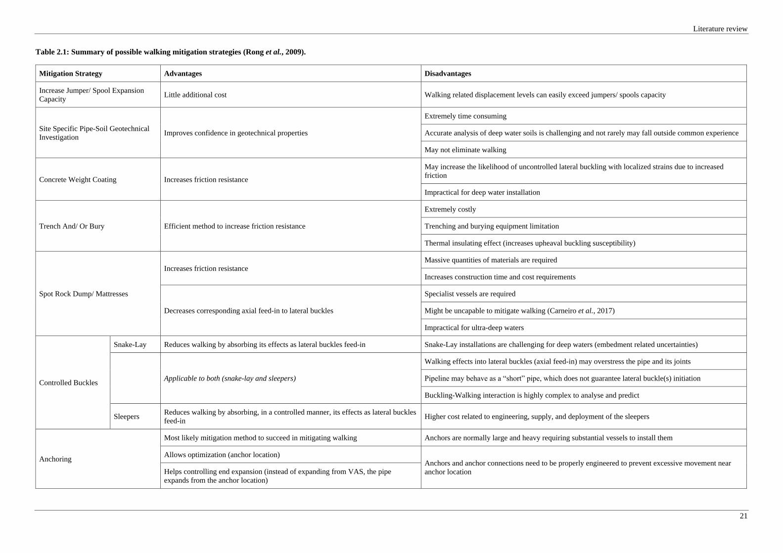
Literature review
21
Table 2.1: Summary of possible walking mitigation strategies (Rong et al., 2009).
Mitigation Strategy Advantages Disadvantages
Increase Jumper/ Spool Expansion
Capacity Little additional cost Walking related displacement levels can easily exceed jumpers/ spools capacity
Site Specific Pipe-Soil Geotechnical
Investigation Improves confidence in geotechnical properties
Extremely time consuming
Accurate analysis of deep water soils is challenging and not rarely may fall outside common experience
May not eliminate walking
Concrete Weight Coating Increases friction resistance
May increase the likelihood of uncontrolled lateral buckling with localized strains due to increased
friction
Impractical for deep water installation
Trench And/ Or Bury Efficient method to increase friction resistance
Extremely costly
Trenching and burying equipment limitation
Thermal insulating effect (increases upheaval buckling susceptibility)
Spot Rock Dump/ Mattresses
Increases friction resistance Massive quantities of materials are required
Increases construction time and cost requirements
Decreases corresponding axial feed-in to lateral buckles
Specialist vessels are required
Might be uncapable to mitigate walking (Carneiro et al., 2017)
Impractical for ultra-deep waters
Controlled Buckles
Snake-Lay Reduces walking by absorbing its effects as lateral buckles feed-in Snake-Lay installations are challenging for deep waters (embedment related uncertainties)
Applicable to both (snake-lay and sleepers)
Walking effects into lateral buckles (axial feed-in) may overstress the pipe and its joints
Pipeline may behave as a “short” pipe, which does not guarantee lateral buckle(s) initiation
Buckling-Walking interaction is highly complex to analyse and predict
Sleepers Reduces walking by absorbing, in a controlled manner, its effects as lateral buckles
feed-in Higher cost related to engineering, supply, and deployment of the sleepers
Anchoring
Most likely mitigation method to succeed in mitigating walking Anchors are normally large and heavy requiring substantial vessels to install them
Allows optimization (anchor location) Anchors and anchor connections need to be properly engineered to prevent excessive movement near
anchor location Helps controlling end expansion (instead of expanding from VAS, the pipe
expands from the anchor location)

Literature review
22
studied. Adding regular concrete mattresses could be inefficient, because the pipeline
might settle into deeper soil levels, due the increase in vertical load in a phenomenon
known as “wedging” (White et al., 2012); and then, the combination of regular concrete
mattresses and “wedging” increased soil axial resistance could not provide sufficient
axial restrain, since regular concrete mattresses would go from membrane tension to
compression, similar to the process studied in Carneiro et al. (2017) for rock dumps.
Therefore, the Pipe-Clamping Mattress (PCM) was created as a solution which instead
of resting on the pipeline, clamps the pipeline, generating a situation where 100% of the
weight increase generate an equivalent axial resistance increase. If necessary, extra
weight might be provided by adding further regular concrete mattresses. Noteworthy
additional stresses in the pipeline wall should be checked against pipeline integrity
requirements, such as those from DNVGL-ST-F101 (DNVGL, 2017b).
Figure 2.10 shows the Pipe-Clamping Mattress (PCM) in four different views: (a) in
deployment above sea level; (b) in deployment below sea level; (c) installed on top of
pipeline; and, (d) installed on pipeline with extra weight concrete mattresses.
The paper then concludes by presenting a performance monitoring over the period of time
between PCMs deployment and after three operational load cycles, which means a period
of time that the pipeline was estimated to walk a distance around 8cm. As can be seen in
Figure 2.11, the resulting displacement during the aforementioned period of time was
found to apparently be zero. In the case the displacements related to walking are very
small, a longer period of time is required for such observations to be made; therefore,
further inspections are programmed, as stressed in Frankenmolen et al. (2017).
Figure 2.11 shows the walking monitoring results after the PCMs installation on the
Malampaya pipeline: (a) right after the PCMs installation – December 2015; and, (b) after
three operational load cycles – January 2016.
2.5 FINAL REMARKS
Pipeline walking is a complex phenomenon that affects pipelines in various operational
conditions such as tensioned end, thermal transients, multiphasic flow, and seabed slopes.
Although pipeline walking has been known and documented for the last two decades, the
efforts of providing broad and general guidance has not kept up to the amount of site-
specific investigations.
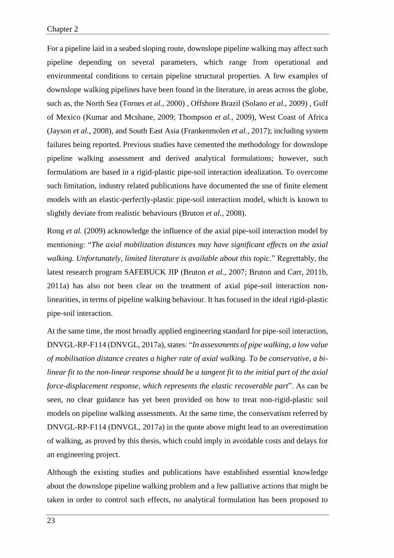
Chapter 2
23
For a pipeline laid in a seabed sloping route, downslope pipeline walking may affect such
pipeline depending on several parameters, which range from operational and
environmental conditions to certain pipeline structural properties. A few examples of
downslope walking pipelines have been found in the literature, in areas across the globe,
such as, the North Sea (Tornes et al., 2000) , Offshore Brazil (Solano et al., 2009) , Gulf
of Mexico (Kumar and Mcshane, 2009; Thompson et al., 2009), West Coast of Africa
(Jayson et al., 2008), and South East Asia (Frankenmolen et al., 2017); including system
failures being reported. Previous studies have cemented the methodology for downslope
pipeline walking assessment and derived analytical formulations; however, such
formulations are based in a rigid-plastic pipe-soil interaction idealization. To overcome
such limitation, industry related publications have documented the use of finite element
models with an elastic-perfectly-plastic pipe-soil interaction model, which is known to
slightly deviate from realistic behaviours (Bruton et al., 2008).
Rong et al. (2009) acknowledge the influence of the axial pipe-soil interaction model by
mentioning: “The axial mobilization distances may have significant effects on the axial
walking. Unfortunately, limited literature is available about this topic.” Regrettably, the
latest research program SAFEBUCK JIP (Bruton et al., 2007; Bruton and Carr, 2011b,
2011a) has also not been clear on the treatment of axial pipe-soil interaction non-
linearities, in terms of pipeline walking behaviour. It has focused in the ideal rigid-plastic
pipe-soil interaction.
At the same time, the most broadly applied engineering standard for pipe-soil interaction,
DNVGL-RP-F114 (DNVGL, 2017a), states: “In assessments of pipe walking, a low value
of mobilisation distance creates a higher rate of axial walking. To be conservative, a bi-
linear fit to the non-linear response should be a tangent fit to the initial part of the axial
force-displacement response, which represents the elastic recoverable part”. As can be
seen, no clear guidance has yet been provided on how to treat non-rigid-plastic soil
models on pipeline walking assessments. At the same time, the conservatism referred by
DNVGL-RP-F114 (DNVGL, 2017a) in the quote above might lead to an overestimation
of walking, as proved by this thesis, which could imply in avoidable costs and delays for
an engineering project.
Although the existing studies and publications have established essential knowledge
about the downslope pipeline walking problem and a few palliative actions that might be
taken in order to control such effects, no analytical formulation has been proposed to

Literature review
24
reliably assess the downslope walking rate for more intricate pipe-soil interaction models.
Additionally, there is still a gap in understanding how such pipe-soil interaction models
and pipe-soil interaction changes due to construction and operational loads impact the
downslope pipeline walking behaviour. The referred knowledge and understanding gaps
can be related to the fact that this is still a new research topic and a little unusual in the
perspective of the number of operational pipelines that never suffered such problems
versus the number of pipelines dealing with this issue. Currently, finite element
modelling is becoming more and more accessible; however, it is still time demanding,
and usually requires a period of time to deliver final results that pipeline engineering
teams simply might not have, especially in early conceptual engineering phases.
Also, there is an increasing demand for probabilistic approaches, in which risk levels are
quantified and the likelihood of different scenarios is estimated. This is important for
design solutions that balance CAPEX and OPEX, such as the ‘wait and see’ approach to
pipeline walking, with planned mitigation in mid- or late-life. In this case, a large number
of simulations must be run to consider all possible operational scenarios. Rapid simple
design tools are required for this approach, rather than finite element analysis. Therefore,
having a quick, accurate and reliable analytical assessment tool is of paramount
importance to deliver solid and secure results.
Finally, this thesis investigates how the current analytical methodology should be
expanded to allow more complex assessments of pipeline walking; which are depending
on the level of pipe-soil interaction complexity (as it has been shown that there are many
more intricate pipe-soil interaction models than rigid-plastic), as well as accounting for
slope variability. Table 2.2 summarises where the different pipe-soil interaction models
are treated in this thesis, along with the slope variability.
Table 2.2: Summary of causes of uncertainty and thesis chapters.
Cause of uncertainty Chapter in thesis
Elastic-perfectly-plastic pipe-soil interaction Chapter 3
Non-linear elastic-plastic pipe-soil interaction Chapter 4
Peaky linear pipe-soil interaction Chapter 5
Non-linear peaky pipe-soil interaction Chapter 6
Slope angle variability Chapter 7

Chapter 2
25
FIGURES
Figure 2.1: Example for field architecture of infield pipelines and production
infrastructure units from White (2011).
Figure 2.2: Effective axial force diagrams for start-up and shutdown loading
phases.

Literature review
26
Figure 2.3: Axial displacement diagrams for start-up and shutdown loading
phases.

Chapter 2
27
Figure 2.4: Rigid-plastic soil behaviour.
Figure 2.5: Axial friction curves (no peak) – adapted from White et al. (2011).
Hypothetical rigid-plastic
pipe-soil interaction models
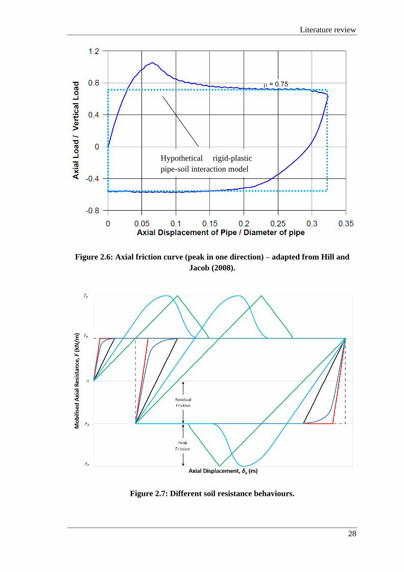
Literature review
28
Figure 2.6: Axial friction curve (peak in one direction) – adapted from Hill and
Jacob (2008).
Figure 2.7: Different soil resistance behaviours.
Hypothetical rigid-plastic
pipe-soil interaction model
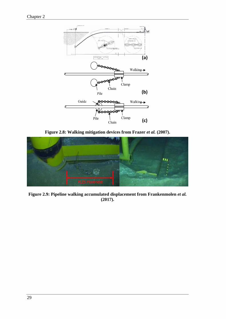
Chapter 2
29
Figure 2.8: Walking mitigation devices from Frazer et al. (2007).
Figure 2.9: Pipeline walking accumulated displacement from Frankenmolen et al.
(2017).

Literature review
30
Figure 2.10: Pipe-clamping mattress from Frankenmolen et al. (2017).
Figure 2.11: Post pipe-clamping mattresses installation walking monitoring from
Frankenmolen et al. (2017).
Chapter 3
31
CHAPTER 3. SIMPLE SOLUTIONS FOR DOWNSLOPE
PIPELINE WALKING ON ELASTIC-PERFECTLY-
PLASTIC SOILS
Chapter context: The published paper presented in this thesis’ chapter details the
research performed to provide the pipeline engineering community with a better
analytical solution that correctly accounts for elastic-perfectly-plastic soil properties. It
explains the required update for the distance between stationary points (initially referred
to as “virtual anchor sections”) and introduces the novel methodology that allows
accurate analytical solutions for elastic-perfectly-plastic pipe-soil interaction.
This chapter contains material that has been prepared for publication as:
Castelo, A., White, D. and Tian, Y., 2019. Simple solutions for downslope pipeline
walking on elastic-perfectly-plastic soils. Journal of Ocean Engineering (Volume 172,
15 January 2019, Pages 671-683).

Elastic-perfectly-plastic soils
32
3.1 ABSTRACT
Pipeline Walking is a phenomenon that occurs when High Pressure and High
Temperature (HPHT) pipelines experience axial instability over their operational
lifetime, and migrate globally in one direction. Existing analytical solutions treat the axial
soil response as rigid-plastic but this does not match the response observed in physical
model tests. In this paper, the authors develop a new analytical strategy using elastic-
perfectly-plastic axial pipe-soil interaction, which leads to more realistic walking rate
predictions. The new analytical methodology is benchmarked with a series of Finite
Element Analyses (FEA), which constitutes a parametric study performed to test the
proposed expressions and improve on the understanding of the influence of axial
mobilisation distance.
3.2 INTRODUCTION
Offshore pipelines are becoming increasingly important as hydrocarbon sources become
more difficult to reach. The global stability of these pipelines in response to operational
loading is a critical issue for the design of oil and gas projects. Such stability comprises
the actions of hydrodynamic loads and the effects of expansion and contraction triggered
by the High-Pressure and High-Temperature (HPHT) operational conditions (usually
imposed by frontier reservoirs), which both constitute the major focus of geotechnical
design for pipelines.
The stability of offshore pipelines is also impacted by the slope of the seabed. New
hydrocarbon sources are commonly located in regions with noticeable depth variations,
in deep water far from shore. These operational conditions are particularly common in
the Gulf of Mexico and Northwest Australia, which are currently in operation, and others
that are in development, such as the Brazilian Pre-Salt and the Arctic Area.
Threats to the integrity of offshore pipelines by the combination of HPHT conditions and
a sloping seabed were first observed by Tornes et al. (2000). Later, industry-supported
research documented many cases of “axial creeping” now known as the “Pipeline
Walking”, as per Carr et al. (2003).
Four mechanisms have been found to incite pipeline walking, as per Bruton et al. (2010):
1. Tension at the end of the flowline;
2. Thermal transients along the line;

Chapter 3
33
3. Multiphase fluid behaviour during restart operations;
4. Seabed slopes along the pipeline route.
Each of the four mechanisms creates an asymmetry in the profile of Effective Axial Force
(EAF). This asymmetry generally results in pipeline walking, by causing unequal pipeline
displacements during cycles of loading and unloading. This paper focuses on the fourth
mechanism.
When pipelines are subjected to changes in temperature and pressure, pipeline walking
can occur. During the Start-Up (SUp) phase, temperature and pressure increments cause
the pipelines to expand axially. This expansion is resisted by the pipe-soil interaction
forces which results in effective compression of the pipeline. When pipelines are
submitted to temperature and pressure reductions in the Shutdown (SDown) phase,
effective tension is induced in the pipeline.
For “long” pipelines, the effective compression build up occurs along a sufficient length
to induce enough mechanical strain to fully compensate for the thermo-mechanical
expansion during the hot stages. For “short” pipelines, the compression build up, due to
soil resistance, is not sufficient to fully compensate for the expansion.
When “short” pipelines are located on a sloping seabed and are not anchored, cycles of
expansion and contraction may cause the pipelines to move with geometric asymmetries
between the start-up and shutdown phases. The sloping seabed generates a component of
weight to act parallel with the seabed in a downslope direction.
Even if pipeline walking is not a limit state in itself, it may present several design
challenges, which include:
• Overstressing of end connections (and in-line connections);
• Loss of tension in a steel catenary riser;
• Increased loading leading to lateral buckling;
• Route instability (curve pull out);
• Need for anchoring mitigation.
Therefore, pipeline walking must be avoided since its consequences may create
downtime and environmental risk, as pointed out by Tornes et al. (2000).
It is known that pre-operational phases may influence the soil resistance during the
operational lifetime of a pipeline through the pre-operational embedment. As noticed by
White et al. (2012), typical pipeline embedments can increase the soil axial resistance by
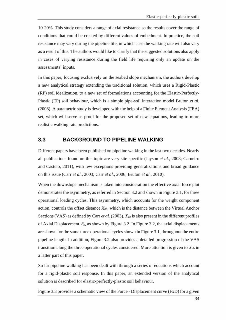
Elastic-perfectly-plastic soils
34
10-20%. This study considers a range of axial resistance so the results cover the range of
conditions that could be created by different values of embedment. In practice, the soil
resistance may vary during the pipeline life, in which case the walking rate will also vary
as a result of this. The authors would like to clarify that the suggested solutions also apply
in cases of varying resistance during the field life requiring only an update on the
assessments’ inputs.
In this paper, focusing exclusively on the seabed slope mechanism, the authors develop
a new analytical strategy extending the traditional solution, which uses a Rigid-Plastic
(RP) soil idealization, to a new set of formulations accounting for the Elastic-Perfectly-
Plastic (EP) soil behaviour, which is a simple pipe-soil interaction model Bruton et al.
(2008). A parametric study is developed with the help of a Finite Element Analysis (FEA)
set, which will serve as proof for the proposed set of new equations, leading to more
realistic walking rate predictions.
3.3 BACKGROUND TO PIPELINE WALKING
Different papers have been published on pipeline walking in the last two decades. Nearly
all publications found on this topic are very site-specific (Jayson et al., 2008; Carneiro
and Castelo, 2011), with few exceptions providing generalizations and broad guidance
on this issue (Carr et al., 2003; Carr et al., 2006; Bruton et al., 2010).
When the downslope mechanism is taken into consideration the effective axial force plot
demonstrates the asymmetry, as referred in Section 3.2 and shown in Figure 3.1, for three
operational loading cycles. This asymmetry, which accounts for the weight component
action, controls the offset distance Xab, which is the distance between the Virtual Anchor
Sections (VAS) as defined by Carr et al. (2003). Xab is also present in the different profiles
of Axial Displacement, δx, as shown by Figure 3.2. In Figure 3.2, the axial displacements
are shown for the same three operational cycles shown in Figure 3.1, throughout the entire
pipeline length. In addition, Figure 3.2 also provides a detailed progression of the VAS
transition along the three operational cycles considered. More attention is given to Xab in
a latter part of this paper.
So far pipeline walking has been dealt with through a series of equations which account
for a rigid-plastic soil response. In this paper, an extended version of the analytical
solution is described for elastic-perfectly-plastic soil behaviour.
Figure 3.3 provides a schematic view of the Force - Displacement curve (FxD) for a given
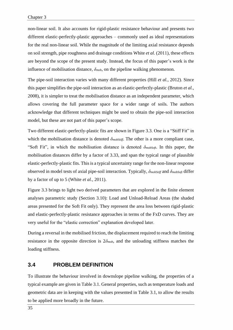
Chapter 3
35
non-linear soil. It also accounts for rigid-plastic resistance behaviour and presents two
different elastic-perfectly-plastic approaches – commonly used as ideal representations
for the real non-linear soil. While the magnitude of the limiting axial resistance depends
on soil strength, pipe roughness and drainage conditions White et al. (2011), these effects
are beyond the scope of the present study. Instead, the focus of this paper’s work is the
influence of mobilisation distance, δmob, on the pipeline walking phenomenon.
The pipe-soil interaction varies with many different properties (Hill et al., 2012). Since
this paper simplifies the pipe-soil interaction as an elastic-perfectly-plastic (Bruton et al.,
2008), it is simpler to treat the mobilisation distance as an independent parameter, which
allows covering the full parameter space for a wider range of soils. The authors
acknowledge that different techniques might be used to obtain the pipe-soil interaction
model, but these are not part of this paper’s scope.
Two different elastic-perfectly-plastic fits are shown in Figure 3.3. One is a “Stiff Fit” in
which the mobilisation distance is denoted δmobStiff. The other is a more compliant case,
“Soft Fit”, in which the mobilisation distance is denoted δmobSoft. In this paper, the
mobilisation distances differ by a factor of 3.33, and span the typical range of plausible
elastic-perfectly-plastic fits. This is a typical uncertainty range for the non-linear response
observed in model tests of axial pipe-soil interaction. Typically, δmobStiff and δmobSoft differ
by a factor of up to 5 (White et al., 2011).
Figure 3.3 brings to light two derived parameters that are explored in the finite element
analyses parametric study (Section 3.10): Load and Unload-Reload Areas (the shaded
areas presented for the Soft Fit only). They represent the area loss between rigid-plastic
and elastic-perfectly-plastic resistance approaches in terms of the FxD curves. They are
very useful for the “elastic correction” explanation developed later.
During a reversal in the mobilised friction, the displacement required to reach the limiting
resistance in the opposite direction is 2δmob, and the unloading stiffness matches the
loading stiffness.
3.4 PROBLEM DEFINITION
To illustrate the behaviour involved in downslope pipeline walking, the properties of a
typical example are given in Table 3.1. General properties, such as temperature loads and
geometric data are in keeping with the values presented in Table 3.1, to allow the results
to be applied more broadly in the future.

Elastic-perfectly-plastic soils
36
Table 3.1: Preliminary example properties.
Parameter Value
Steel Outside Diameter, OD 0.3239m
Steel Wall Thickness, t 0.0206m
Length, L 5000m
Seabed Slope, β 2.0°
Temperature Variation, ΔT 100°C
Pipe Submerged Weight, W 0.8kN/m
Friction factor, μ 0.5
Steel Young's Modulus, E 2.07x10¹¹Pa
Steel Poisson Coefficient, ν 0.3
Steel Thermal Expansion Coefficient, α 1.165x10⁻⁵°C-1
Mobilisation Distance for Stiff Fit, δmobStiff 0.03OD
Mobilisation Distance for Soft Fit, δmobSoft 0.10OD
3.5 RIGID-PLASTIC ANALYTICAL SOLUTIONS
The current design practice – in accordance with Carr et al. (2006) – involves three
different calculation steps to analytically assess pipeline walking rate under the influence
of seabed slope.
The first calculation step assesses the distance between the VASs, Xab,RP, as presented by
equation (3.1):
𝑋𝑎𝑏,𝑅𝑃 =𝐿 tan𝛽
𝜇 (3.1)
The second calculation step assesses the change in force in the pipeline, ΔSS,RP, between
start-up and shutdown phases over the length of the pipeline denoted by Xab,RP:
𝛥𝑆𝑆,𝑅𝑃 = −𝑊𝐿(𝜇 cos 𝛽 − |sin 𝛽|) (3.2)
This change in force, occurring over the distance Xab,RP, creates the asymmetry in axial
movement of the pipeline over a single temperature cycle, which is the origin of the
walking behaviour. The walking distance per cycle, WRRP can then be determined in the

Chapter 3
37
third and last step by combining equations (3.1) and (3.2):
𝑊𝑅𝑅𝑃 =[|𝛥𝑃| +𝑊𝐿|sin 𝛽| −𝑊𝐿𝜇 cos 𝛽]𝐿 tan 𝛽
𝐸𝐴𝜇 (3.3)
where ΔP is the change in fully constrained force, as per Carr et al. (2003).
However, equation (3.3) can be entirely rewritten as:
𝑊𝑅𝑅𝑃 =(∆𝑆𝑆,𝑅𝑃 − ∆𝑃)𝑋𝑎𝑏,𝑅𝑃
𝐸𝐴 (3.4)
Equation (3.4) might also be rewritten more fundamentally as:
𝑊𝑅𝑅𝑃 = −1
𝐸𝐴(∫ (∆𝑃)𝑑𝑥
𝑉𝐴𝑆𝑆𝑈𝑝,𝑅𝑃
𝑉𝐴𝑆𝑆𝐷𝑜𝑤𝑛,𝑅𝑃
−∫ (∆𝑆𝑠)𝑑𝑥𝑉𝐴𝑆𝑆𝑈𝑝,𝑅𝑃
𝑉𝐴𝑆𝑆𝐷𝑜𝑤𝑛,𝑅𝑃
) (3.5)
The rigid-plastic soils equation (3.5) is equal to ΔSS,RP integral (see Section 2.2.1 for
additional steps in this analysis).
The analytical solutions shown above – equations (3.1), (3.2), (3.3), (3.4) and (3.5) – have
been used to calculate pipeline walking rates based on the rigid-plastic assumption. Table
3.2 summarizes the analytical results for Carr et al. (2006) based on the general pipeline
properties given in Table 3.1.
Table 3.2: Rigid-plastic analytical results.
Parameter Value
Xab,RP 349.208m
ΔSS,RP -1859.184kN
WRRP 0.247m/cycle
3.6 FINITE ELEMENT ANALYSES METHODOLOGY
The finite element model used for this paper was a simplified model of a straight pipeline
laid on a uniformly sloping seabed using the parameters presented in Table 3.1.
The pipeline was represented by 5001 nodes connected by 5000 equal Euler Bernoulli
beams (B33 elements in Abaqus) representing the 5000m long pipeline. Each element,
therefore, is 1 metre in length.

Elastic-perfectly-plastic soils
38
The pipe-soil interaction was modelled as elastic-perfectly-plastic spring-slider elements
connected to each pipeline node. The spring-slider elements were developed as User
Elements (UELs) described by a subroutine in FORTRAN.
Figure 3.4 shows an overall sketch of the finite element model. It presents the uniformly
sloped pipeline and provides information about the boundary conditions imposed to all
nodes, which can only displace along the local longitudinal axis given the UEL reaction.
The spring-slider provided a constant stiffness between zero and a certain prescribed
displacement (mobilisation distance) and a corresponding force (according to Hooke’s
law). If the displacement level exceeds the mobilisation distance, the UEL provides zero
tangent stiffness and a constant force, as per the plastic plateau. On reversal, the same
stiffness is considered, until the resultant force equals the plastic plateau.
The UEL behaviour shown in Figure 3.3 is presented in terms of the loads normal to the
seabed.
This paper considers only weight and temperature as the loads acting on the pipeline.
Pressure was disregarded since it can be equally represented by an extra temperature load
(Hobbs, 1984).
The effect of the uniform slope is considered as an axial or longitudinal load equivalent
to the component of the pipeline weight, as given by:
𝑊𝑐𝑜𝑚𝑝 = 𝑊 sin 𝛽 (3.6)
The temperature loads were considered by temperature increments applied directly to the
pipeline. Operational cycling was performed taking into account the steady operational
profile (start-up) and the rest condition (shutdown).
The analyses were performed by:
1. Generating pipeline (nodes and elements) geometry;
2. Applying boundary conditions and UEL properties;
3. Applying gravity to pipeline;
4. Applying temperature increment (start-up temperature);
5. Applying temperature decrement (shutdown temperature);
6. Iterating phases 4 and 5 (9 times);
7. Extracting results from simulations’ outputs.

Chapter 3
39
3.7 FINITE ELEMENT ANALYSES COMPARISON WITH
RIGID-PLASTIC SOLUTION
Figure 3.5 presents the effective axial force responses for the EP Stiff and the Soft fits;
while Figure 3.6 and Figure 3.7 present the δx plots for the EP Stiff Fit and the EP Soft
Fit, respectively.
From the rigid-plastic case (Bruton et al., 2010), the zero displacement point is exactly
the same as the maximum effective axial force point (Table 3.3). However, the elastic-
perfectly-plastic FE results show that the point of zero displacement no longer coincides
with the point of maximum effective axial force.
Table 3.3: Elastic-perfectly-plastic FEA results.
Parameter Source Value
Xab,RP EAF & δx - Figure 3.1, Figure 3.2 and equation (3.1) 349m
Xab,EP_Stiff EAF - Figure 3.5
347m
Xab,EP_Stiff δx - Figure 3.6 321m
Xab,EP_Soft EAF - Figure 3.5 343m
Xab,EP_Soft δx - Figure 3.7 258m
As defined by Carr et al. (2003), the VASs are the sections where the δx is zero and for
the rigid-plastic soil response the VAS and the point of highest effective axial force
coincide, which makes the solution proposed by Carr et al. (2006) perfectly applicable
for rigid-plastic soils.
However, elastic-perfectly-plastic soil behaviour complicates the Xab definition, as used
by Bruton et al. (2010) and Carr et al. (2006). Thus, Xab needs to be redefined. In addition,
the points on the pipe with zero net movement (δx=0) over the period of temperature
change (either start-up or shutdown) are not stationary over this period but they move
initially in one direction then return to their original position. Here, these sections with
zero net movement are called “Stationary Points” (SP). While δx during the temperature
change phase is ideally zero for these sections, in fact they move through a cycle of
displacement and return to the original position at the end of the expansion or contraction.
Figure 3.8 shows the mentioned behaviour for stationary points during some load phases
(for the EP Stiff Fit) along with a schematic plot of the finite element model to clarify the

Elastic-perfectly-plastic soils
40
location of these stationary points. It is important to highlight that there will be one
stationary point per loading phase, which will remain at the same pipeline Kilometre Post
(KP), represented by the model nodes, as long as the conditions (temperature, soil,
geometry, etc.) also remain the same during the operational lifetime.
In the following analysis, Xab is defined as the distance between the stationary points.
This definition is more useful than the distance between the maxima in the effective axial
force profiles because the walking rate per cycle is fundamentally related to the integrated
change in effective axial force in the length of pipe between the stationary points.
3.8 XAB FOR ELASTIC-PERFECTLY-PLASTIC SOIL
The three different values for Xab (Xab,RP, Xab,EP_Stiff and Xab,EP_Soft) are compared to δmob,
in Figure 3.9, which shows the linear dependence of Xab on δmob. Imagining there is a
certain level of mobilisation distance which makes Xab to be equal to zero (and
consequently ceases the walking pattern), represented by δnull, which will be given later
in this paper, the following linear equation might be written:
𝑋𝑎𝑏,𝐸𝑃 = 𝑋𝑎𝑏,𝑅𝑃 (1 −𝛿𝑚𝑜𝑏𝛿𝑛𝑢𝑙𝑙
) (3.7)
This definition of Xab,EP for use in equation (3.4) is now defined for elastic-perfectly-
plastic soils; thus the only element missing is ΔSS,EP to analytically derive the elastic-
perfectly-plastic walking rate.
3.9 ΔSS FOR ELASTIC-PERFECTLY-PLASTIC SOIL
For rigid-plastic soils, ΔSS can be obtained directly from the basic problem parameters
using equation (3.2). For elastic-perfectly-plastic soils, however, ΔSS is not straight
forward, as the effective axial force profile is not triangular. For this reason, the effective
axial force equations need to be redefined by adopting the solution for an elastic column
compressed within an elastic medium, as used in the analysis of piles. This leads to a
second order linear differential equation which represents the displacement, δ, along the
longitudinal axis, x, as shown by equation (3.8) from Randolph (1977).
𝛿 = 𝐾1𝑒𝜉𝑥 + 𝐾2𝑒
−𝜉𝑥 (3.8)
where K1 and K2 are arbitrary constants, and ξ is exponential factor. More detail about
these parameters is given in Appendix A.

Chapter 3
41
However, before solving the differential equation, the boundary conditions among the
different behaviour patterns along the pipe route need to be defined.
Table 3.4 presents the physical boundaries that should be considered for the elastic-
perfectly-plastic effective axial force calculation, which segregates the different zones of
the pipeline. For pipeline zones Z1 and Z4 effective axial force is equivalent to the rigid-
plastic solution with straight line behaviour and constant gradient – equations (3.9) and
(3.10):
Table 3.4: Pipeline zoning.
Zone Initial KP Final KP
Z1 0 x12
Z2 x12 x23
Z3 x23 x34
Z4 x34 L
𝑊(μcos 𝛽 + sin 𝛽) (3.9)
𝑊(μcos 𝛽 − sin 𝛽) (3.10)
In contrast to zones Z1 and Z4, the behaviour of the Z2 and Z3 central zones (in the
vicinity of the highest effective axial force section), creates two different parabolic curves
(within the effective axial force plot), whose gradients vary from 0 to the values given by
equations (3.9) and (3.10).
Figure 3.10 presents a schematic plot accounting the physical boundaries and also the
revised solution for a hypothetic case.
3.9.1 δx Boundary Conditions
Considering the physical boundaries and their outcomes in terms of displacement, δ, it is
clear that displacements at x23 are zero, while at x12 and x34 displacements are equal to
δmob, where the soil resistance is fully mobilised.
3.9.2 Effective Axial Force Boundary Conditions
From Figure 3.10 it is clear that some boundary conditions must be respected when
obtaining the analytical elastic-perfectly-plastic effective axial force response; which are:
• Continuity of slope for the three zone boundaries;

Elastic-perfectly-plastic soils
42
• Continuity of effective axial force at the three zone boundaries.
These effective axial force boundary conditions might be rewritten as shown in Table
3.5.
Table 3.5: EAF boundary conditions.
x coordinate EAF 𝑑𝐸𝐴𝐹
𝑑𝑥
0 0 𝑊(μcos 𝛽 + sin 𝛽)
x12 𝑥12[𝑊(μcos 𝛽 + sin 𝛽)] 𝑊(μcos 𝛽 + sin 𝛽)
x23 ? 0
x34 𝑥34[𝑊(μcos 𝛽 − sin 𝛽)] 𝑊(μcos 𝛽 − sin 𝛽)
L 0 𝑊(μcos 𝛽 − sin 𝛽)
The question mark in Table 3.5 might only be answered after the differential equation is
solved and an expression for the effective axial force calculation is reached.
Hence, a general equation was written as follows:
(𝑑𝐹
𝑑𝑥)𝑥=
{
𝜇𝑊𝑍1, 𝛿𝑥 ≤ −𝛿𝑚𝑜𝑏
(𝜇𝑊𝑍1
𝛿𝑚𝑜𝑏) 𝛿𝑥, −𝛿𝑚𝑜𝑏 < 𝛿𝑥 < 0
(𝜇𝑊𝑍4
𝛿𝑚𝑜𝑏) 𝛿𝑥, 0 < 𝛿𝑥 < 𝛿𝑚𝑜𝑏
𝜇𝑊𝑍4, 𝛿𝑥 ≥ 𝛿𝑚𝑜𝑏
(3.11)
where µWZ? represents the soil resistance plus or minus, depending on the zone
considered, the weight component acting on the pipe due to the seabed slope.
3.9.3 Effective Axial Force Pipe Differential Equation
Observing the effective axial force boundary conditions and their implications, the
effective axial force differential equation could be written as:

Chapter 3
43
𝐸𝐴𝐹(𝑥)
=
{
𝜇𝑊𝑍1 ∗ 𝑥, 0 ≤ 𝑥 ≤ 𝑥12
𝐸𝐴𝐹(𝑥12) +√𝐸𝐴𝜇𝑊𝑍1
𝛿𝑚𝑜𝑏[𝐾1(𝑥)(𝑒
𝜉𝑍1𝑠𝑖 − 𝑒𝜉𝑍1𝑠𝑖−1) + 𝐾2(𝑥)(𝑒−𝜉𝑍1𝑠𝑖−1 − 𝑒−𝜉𝑍1𝑠𝑖)] ,
𝑥12 < 𝑥 ≤ 𝑥23
𝐸𝐴𝐹(𝑥23) +√𝐸𝐴𝜇𝑊𝑍4
𝛿𝑚𝑜𝑏[𝐾1(𝑥)(𝑒
𝜉𝑍4𝑠𝑖 − 𝑒𝜉𝑍4𝑠𝑖−1) + 𝐾2(𝑥)(𝑒−𝜉𝑍4𝑠𝑖−1 − 𝑒−𝜉𝑍4𝑠𝑖)] ,
𝑥23 ≤ 𝑥 < 𝑥34𝜇𝑊𝑍4 ∗ (𝐿 − 𝑥), 𝑥34 ≤ 𝑥 ≤ 𝐿
(3.12)
See Appendix A for details on the mathematical development of equation (3.8) towards
equation (3.12).
With equation (3.12) the unknown values in Table 3.5 are derived and the full effective
axial force profiles can be deduced via iteration on the position of x23.
This solution scheme for the effective axial force profile for elastic-perfectly-plastic soils
leads to the last step of the new calculation approach.
3.9.4 ΔSS Revision
ΔSS can be directly described as the summation of areas, as given by equation (3.13), and
as schematically shown by Figure 3.11.
∫ (∆𝑆𝑠)𝑑𝑥𝑆𝑃𝑆𝑈𝑝
𝑆𝑃𝑆𝐷𝑜𝑤𝑛
= −(|𝐴𝑟𝑒𝑎1| + |𝐴𝑟𝑒𝑎2| + |𝐴𝑟𝑒𝑎3| + |𝐴𝑟𝑒𝑎4|) (3.13)
where each area represents the partial integral of effective axial force in terms of x
coordinate accounting the physical boundaries as seen in Figure 3.11.
3.10 WALKING RATE FOR ELASTIC-PERFECTLY-PLASTIC
SOIL
Based on the above expressions, the walking rate for elastic-perfectly-plastic soils can be
derived. Taking into account equation (3.5), the general modifications are:
𝑊𝑅𝐸𝑃 = −1
𝐸𝐴(∫ (∆𝑃)𝑑𝑥
𝑆𝑃𝑆𝑈𝑝,𝐸𝑃
𝑆𝑃𝑆𝐷𝑜𝑤𝑛,𝐸𝑃
−∫ (∆𝑆𝑠)𝑑𝑥𝑆𝑃𝑆𝑈𝑝,𝐸𝑃
𝑆𝑃𝑆𝐷𝑜𝑤𝑛,𝐸𝑃
) (3.14)
To validate this revised expression for WREP, a parametric finite element analyses study
was conducted.

Elastic-perfectly-plastic soils
44
3.11 FINITE ELEMENT ANALYSES PARAMETRIC STUDY
The parametric study used a range of values for the following parameters:
• Pipeline length;
• Pipeline submerged weight;
• Friction factor;
• Route overall slope.
For these core properties three different values were attributed for each, resulting in 81
different combinations. The different values used are shown in Table 3.6.
Table 3.6: FEA parametric variables.
Parameter Value A Value B Value C
Length (m) 3000 4000 5000
Weight (kN/m) 0.4 0.6 0.8
Friction (-) 0.5 0.7 0.9
Slope (°) 1 2 3
Since the focus of this paper is the influence of axial mobilisation distance, eight different
values of δmob were considered, in terms of pipeline steel outside diameter (OD),
(0.03OD, 0.05OD, 0.06OD, 0.10OD, 0.15OD, 0.20OD, 0.33OD and 0.50OD), giving a
total of 648 cases.
All 648 cases were modelled using the same finite element analyses solution. All
respected the general behaviour for the pipeline walking phenomenon as expected
(including the revised solutions).
Figure 3.12 presents the finite element analyses results for Xab,EP plotted against δmob for
the 1° seabed slope while Figure 3.13 compares Xab achieved through finite element
analyses and the equations proposed in this paper. Figure 3.14, Figure 3.15, Figure 3.16
and Figure 3.17 provide the same results for 2° and 3° seabed slopes, respectively.
In Figure 3.13, Figure 3.15 and Figure 3.17 the results were plotted along with a line
representing the equation (3.7) for each case. The finite element analyses results clearly
validate equation (3.7).
At this stage, the results obtained for Xab using the suggested formulation (equation (3.7))

Chapter 3
45
and the finite element analyses’ results were statistically analysed. For the 1° slope, the
coefficient of determination, R2, is equal to 0.986; whilst for 2° and 3°, R2 is equal to
0.997 and 0.998, respectively. It is clear that the proposed methodology has a very strong
accuracy. The authors also looked into the reason for the difference noticed in the 1°
models, and it was found that some finite element models had an accidental limitation in
terms of mesh. This generated a numerical noise that was reflected in the overall results.
The noise can be eliminated through the use of a finer mesh in the models, thus retaining
their applicability to any slope.
Figure 3.18 shows the finite element model results for WREP plotted against δmob for the
1° seabed slope. Figure 3.20 and Figure 3.22 give the same results for 2° and 3° seabed
slopes. Figure 3.19, Figure 3.21 and Figure 3.23 present the comparison between finite
element analyses and equation results.
Again, applying some statistics to the results shown by Figure 3.19, Figure 3.21 and
Figure 3.23, the coefficient of determination, R2, was calculated to be 0.985 (for 1° slope),
0.997 (for 2° slope) and 0.999 (for 3° slope). These results confirm the level of accuracy
of the findings of this paper and reinforce the applicability of the proposed methodology.
As it can be seen, the analytical expressions shown in Sections 3.8, 3.9 and 3.10 agree
closely with the finite element analyses results, as shown by the plots from Figure 3.12
to Figure 3.23.
Hence, for any straight pipeline resting on any sloping seabed with an elastic-perfectly-
plastic soil we can conclude that the realistic walking rate might be written as:
𝑊𝑅𝐸𝑃 = 𝑊𝑅𝑅𝑃 − 𝐶𝑜𝑟𝑟𝐸𝑃 (3.15)
where the elastic correction, CorrEP, is equivalent to:
𝐶𝑜𝑟𝑟𝐸𝑃 = 2(𝐴𝑟𝑒𝑎𝑈𝑛𝑙𝑜𝑎𝑑−𝑅𝑒𝑙𝑜𝑎𝑑
𝛥𝐹) (3.16)
The unload-reload area and the ΔF are exemplified in Figure 3.3. Then, considering the
single-spring elastic-perfectly-plastic approach, the entity elastic correction equals:
𝐶𝑜𝑟𝑟𝐸𝑃 = 2(2𝜇𝑊 cos 𝛽 𝛿𝑚𝑜𝑏2𝜇𝑊 cos 𝛽
) = 2𝛿𝑚𝑜𝑏 (3.17)
Equation (3.17) also allows us to define the non-walking mobilisation distance, δnull, to
be:

Elastic-perfectly-plastic soils
46
𝛿𝑛𝑢𝑙𝑙 =𝑊𝑅𝑅𝑃2
(3.18)
3.12 CONCLUSIONS & FINAL REMARKS
This paper provides an analytical solution that solves pipeline walking problems for
elastic-perfectly plastic (EP) pipe-soil response, benchmarked and validated against finite
element analyses performed with an elastic-perfectly-plastic user-defined element. These
revised solutions improve understanding of the parameters involved in elastic-perfectly-
plastic soil behaviour for pipeline walking assessment. The paper resolves how the
fundamental solution for rigid-plastic pipe-soil interaction requires expansion to allow
for elasticity. It is shown that the “Stationary Points”, which have zero movement during
changes in the pipe temperature, do not coincide with the positions of maximum effective
axial force (EAF). This is an important distinction compared to the rigid-plastic solution,
in which the term “Virtual Anchor Point” is well-established as both the Stationary Point
and the position of maximum effective axial force. Using the revised Stationary Points,
the resulting mathematical proof shows the swept area within the effective axial force
plot during a change in temperature remains a valid method to assess the pipeline
expansion and contraction and therefore the pipeline walking. Relative to the rigid-plastic
solution, the correction for elasticity is equivalent to the loss in area represented by the
Unload-Reload Area inherent to the FxD soil curve.
Common solutions for pipeline walking, in which the soil is treated as rigid-plastic,
invariably derive overestimates of walking action. Besides being unrealistic, a magnified
walking rate can be onerous for projects, leading to additional effort and cost to mitigate
pipeline walking.
Therefore, it is important to identify and apply realistic soil properties, and the solution
in this paper allows the elastic-perfectly-plastic rather than rigid-plastic approach to be
used.
The walking mechanism, explored in this paper, can now be assessed by a set of analytical
expressions for walking evaluation, based on the general problem properties, such as,
overall route slope, temperature variation and pipeline geometric data. These expressions
were validated against a finite element analyses set.

Chapter 3
47
FIGURES
Figure 3.1: EAF diagrams for SUp and SDown phases.

Elastic-perfectly-plastic soils
48
Figure 3.2: δx diagrams for SUp and SDown phases.

Chapter 3
49
Figure 3.3: Rigid-plastic & elastic-plastic soil responses.
Figure 3.4: Finite element model sketch.

Elastic-perfectly-plastic soils
50
Figure 3.5: EAF plot (zoom).

Chapter 3
51
Figure 3.6: δx plot for Stiff Fit (zoom).
Figure 3.7: δx plot for Soft Fit (zoom).

Elastic-perfectly-plastic soils
52
Figure 3.8: x coordinate for the stationary points.
Figure 3.9: Xab,EP results against δmob.

Chapter 3
53
Figure 3.10: Schematic plot accounting physical boundaries.
Figure 3.11: Schematic EAF plot with the partial areas highlight.

Elastic-perfectly-plastic soils
54
Figure 3.12: Xab,EP results for 1° slope.
Figure 3.13: Xab,EP results – numerical & calculated for 1° slope.
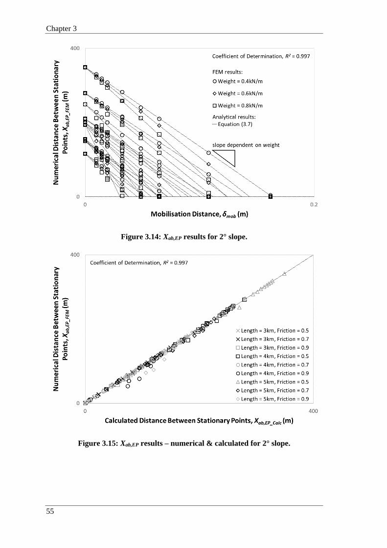
Chapter 3
55
Figure 3.14: Xab,EP results for 2° slope.
Figure 3.15: Xab,EP results – numerical & calculated for 2° slope.

Elastic-perfectly-plastic soils
56
Figure 3.16: Xab,EP results for 3° slope.
Figure 3.17: Xab,EP results – numerical & calculated for 3° slope.

Chapter 3
57
Figure 3.18: WREP results for 1° slope.
Figure 3.19: WREP results – numerical & calculated for 1° slope.

Elastic-perfectly-plastic soils
58
Figure 3.20: WREP results for 2° slope.
Figure 3.21: WREP results – numerical & calculated for 2° slope.
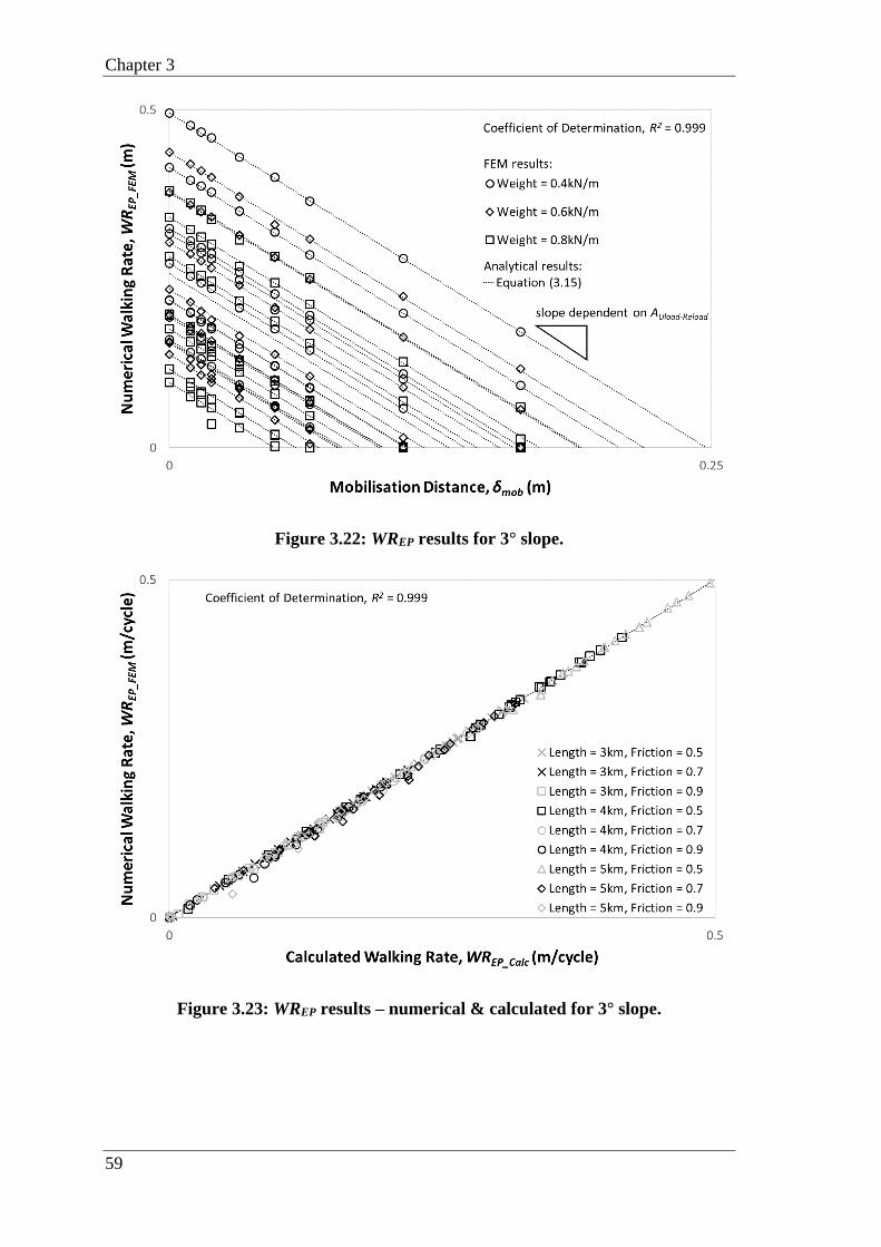
Chapter 3
59
Figure 3.22: WREP results for 3° slope.
Figure 3.23: WREP results – numerical & calculated for 3° slope.

Non-linear elastic-plastic soils
60
CHAPTER 4. SOLVING DOWNSLOPE PIPELINE
WALKING ON NON-LINEAR ELASTIC-PLASTIC SOILS
Chapter context: This thesis’ chapter presents the research done to generate an improved
analytical solution to properly account for non-linear elastic-plastic soil properties. It
establishes how a non-linear elastic-plastic soil behaviour can be satisfactorily
approximated to an elastic-perfectly-plastic pipe-soil interaction model. It clarifies that
certain levels of mobilization distance might impede the pipeline walking phenomenon
from happening. Finally, it concludes by showing adjustments to the analytical solutions
that improve the results’ accuracy when non-linear elastic-plastic soils are considered.
This chapter contains material that has been prepared for publication as:
Castelo, A., White, D. and Tian, Y., in press. Solving downslope pipeline walking on
non-linear elastic-plastic soils. Journal of Marine Structures (submitted to journal)
Chapter 4
61
4.1 ABSTRACT
Over their operational lifetime, offshore pipelines can experience an accumulation of
axial movement, referred to as “pipeline walking”, due to high pressures and
temperatures resulting in asymmetric expansion and contraction. Treating the axial soil
response as elastic-perfectly-plastic, as is conventional in design, does not fully account
for the pipe-soil interaction response observed in physical model tests and can give
inaccurate estimates of walking rate per cycle. In this paper, modifications to the elastic-
perfectly-plastic approach are made to give a new set of formulations involving non-
linear axial pipe-soil interaction, which leads to more accurate walking rate predictions.
It is shown that an equivalent elastic-perfectly-plastic model can be defined from the non-
linear response. This equivalent approach allows existing analytical expressions for
walking rate on elastic-perfectly-plastic soil to be applied, therefore providing an efficient
new design tool. This work is based on a parametric study using finite element analysis,
focused on the case of downslope pipeline walking.
4.2 INTRODUCTION
Offshore pipelines have been increasingly employed as the industry further explores deep
water hydrocarbon reservoirs. The stability of these pipelines is dependent on a number
of factors, including environmental and geotechnical aspects. For example, a pipeline
expands and contracts due to temperature and pressure changes. When the pipeline is on
a seabed slope, these changes become asymmetric, which might lead to net movement in
one direction – a phenomenon known as pipeline walking. This phenomenon increases
cost and risk and may cause severe consequences through the overstressing of
connections, altered loading and strain in any engineered lateral buckles and an increased
need for anchoring (Bruton et al., 2010). Therefore, properly quantifying pipeline
walking is necessary to reduce the risk of a loss of production and damage to the
environment (Tornes et al., 2000). If engineered well, the system can benefit from
significant cost-savings.
Currently, pipeline walking is often estimated during the design phase of offshore
pipelines using analytical formulae. These analyses need to account for various factors,
such as soil behaviour, seabed slope and operational temperature. Providing accurate
estimates for high-pressure and high-temperature operational conditions for downslope
pipelines is particularly relevant to the industry as such conditions are commonly found

Non-linear elastic-plastic soils
62
in major oil and gas regions, including the Gulf of Mexico, West Africa and Northwest
Australia, as well as frontier locations, including the Brazilian Pre-Salt and the Arctic
area. However, current analytical formulae used by the industry are idealised, which can
produce inaccurate walking rates and further analyses are done to account for the known
limitations, such as the assumption of a linear elastic-perfectly-plastic form of pipeline-
seabed interaction.
When the pipeline walking tendency is identified through the analytical formulae, time
demanding and costly finite element analyses are performed to confirm the walking
behaviour and provide a reliable walking rate. However, as demonstrated by Castelo et
al., (2019), if more appropriate soil behaviours are accounted for in the initial analytical
formulae, the industry could avoid unnecessary additional expensive steps.
The formulation identified by Castelo et al., (2019) assume an elastic-perfectly-plastic
soil model, which requires improvement to realistically represent real soil conditions, and
thus generate more accurate pipeline walking rates.
This paper examines the influence on pipeline walking of a non-linear elastic-plastic soil
response, to see the influence of adopting a realistic soil condition. It begins with a
literature review of current methods used for estimating the walking rate for rigid-plastic
and elastic-perfectly-plastic soil behaviour. It then sets out a theoretical framework for
estimating the walking rate for non-linear elastic-plastic soils. Next, finite element
analyses are conducted to confirm this theoretical framework for non-linear elastic-
plastic soil types. Finally, this paper generates a solution that allows the non-linearity to
be captured in an analytical formula, so that the requirement for costly finite element
analysis can be reduced.
4.3 BACKGROUND TO PIPELINE WALKING
4.3.1 Downslope mechanism
For a sloping seabed, the effective axial force plot of a fully mobilised pipeline shows an
asymmetry between the start-up and shutdown phases, as illustrated in Figure 4.1, where
the pipe-soil interaction is considered as rigid-plastic. This asymmetry creates a
separation Xab between the Virtual Anchor Sections (VASs), which for rigid-plastic soils
coincide with the points of maximum absolute effective axial force, as proved by Castelo
et al. (2019). Xab is then related to the net axial displacement, δx, from a cycle of start-up
and shutdown phases as shown by Figure 4.2. The asymmetry in the profile of effective

Chapter 4
63
axial force is currently understood by the industry to be the root cause of pipeline walking,
as it tends to generate unbalanced movements during different loading cycles (start-up
and shutdown phases).
For soil conditions that are not rigid-plastic, Xab is not related to the point of maximum
effective axial force. The separation Xab is exclusively related to the stationary points, as
explained in further detail by Castelo et al. (2019).
4.3.2 Pipe-soil response
While the pipe-soil response has traditionally been treated in pipe walking analyses as
rigid-plastic or elastic-perfectly-plastic, in reality most soils behave non-linearly.
Figure 4.3 shows a typical axial force-displacement response for four different types of
pipe-soil interaction: rigid-plastic, non-linear elastic-plastic and two different elastic-
perfectly-plastic approximations (soft and stiff). The unload-reload area in the figure
represents the area loss in the pipe-soil response between the rigid-plastic and the non-
linear elastic-plastic models. This is explored further in this paper, where a “non-linear
elastic correction” is proposed. This allows the non-linear elastic-plastic response to be
simplified into an equivalent linear elastic-perfectly-plastic response, for use in analytical
solutions of walking rate.
4.4 PROBLEM DEFINITION
To illustrate the method being proposed in this research, this paper will use two cases.
The first case is for dual-spring strategy and the second is for multi-spring strategy, to
better mimic realistic pipe-soil interactions. In both cases, multiple elastic-perfectly-
plastic pipe-soil responses have been combined to generate the non-linear elastic-plastic
response.
Downslope pipeline walking is dependent on three types of properties: environmental,
operational and those of the pipeline. Our parametric studies use typical parameter ranges
for these three properties; the multi-spring case has slightly more demanding parameters,
to test the rigour of our proposed methodology.
For the dual-spring case, the environmental parameters include seabed slope and friction
coefficient, taken to be 2° and 0.5, respectively in the first examples shown, but with a
wider range used later to generalise the solutions. The operational parameters include
temperature variation and pipe submerged weight, assumed to be 100°C and 0.8kN/m,

Non-linear elastic-plastic soils
64
respectively. The physical pipeline properties include steel outside diameter, steel wall
thickness and length, taken to be 0.3239m, 0.0206m and 5000m, respectively.
The multi-spring case has a steeper slope, assumed to be 3°, lighter pipe submerged
weight of 0.4kN/m and the exact same physical pipeline properties. The full list of
properties and the parameters used in our study are provided in Table 4.1 and Table 4.2.
Table 4.1: Preliminary example properties – Dual-Spring UEL.
Parameter Value
Steel Outside Diameter, OD 0.3239m
Steel Wall Thickness, t 0.0206m
Length, L 5000m
Seabed Slope, β 2.0°
Temperature Variation, ΔT 100°C
Pipe Submerged Weight, W 0.8kN/m
Friction coefficient, μ 0.5
Steel Young's Modulus, E 2.07x10¹¹Pa
Steel Poisson Coefficient, ν 0.3
Steel Thermal Expansion Coefficient, α 1.165x10⁻⁵°C-1
Mobilisation Distance for Spring S1, δmobS1/OD 0.030
Plastic Force for Spring S1, FS1 0.259842kN
Mobilisation Distance for Spring S2, δmobS2/OD 0.100
Plastic Force for Spring S2, FS2 0.139915kN
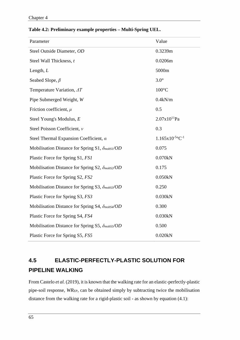
Chapter 4
65
Table 4.2: Preliminary example properties – Multi-Spring UEL.
Parameter Value
Steel Outside Diameter, OD 0.3239m
Steel Wall Thickness, t 0.0206m
Length, L 5000m
Seabed Slope, β 3.0°
Temperature Variation, ΔT 100°C
Pipe Submerged Weight, W 0.4kN/m
Friction coefficient, μ 0.5
Steel Young's Modulus, E 2.07x10¹¹Pa
Steel Poisson Coefficient, ν 0.3
Steel Thermal Expansion Coefficient, α 1.165x10⁻⁵°C-1
Mobilisation Distance for Spring S1, δmobS1/OD 0.075
Plastic Force for Spring S1, FS1 0.070kN
Mobilisation Distance for Spring S2, δmobS2/OD 0.175
Plastic Force for Spring S2, FS2 0.050kN
Mobilisation Distance for Spring S3, δmobS3/OD 0.250
Plastic Force for Spring S3, FS3 0.030kN
Mobilisation Distance for Spring S4, δmobS4/OD 0.300
Plastic Force for Spring S4, FS4 0.030kN
Mobilisation Distance for Spring S5, δmobS5/OD 0.500
Plastic Force for Spring S5, FS5 0.020kN
4.5 ELASTIC-PERFECTLY-PLASTIC SOLUTION FOR
PIPELINE WALKING
From Castelo et al. (2019), it is known that the walking rate for an elastic-perfectly-plastic
pipe-soil response, WREP, can be obtained simply by subtracting twice the mobilisation
distance from the walking rate for a rigid-plastic soil - as shown by equation (4.1):
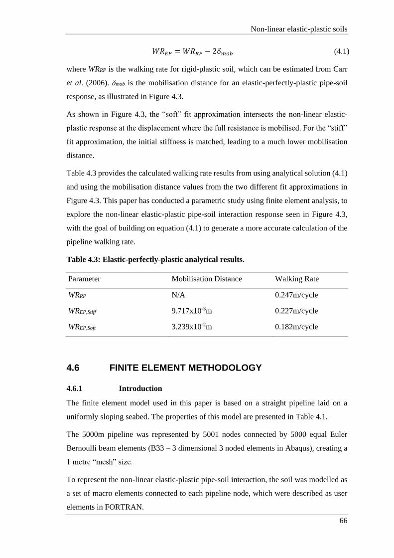
Non-linear elastic-plastic soils
66
𝑊𝑅𝐸𝑃 = 𝑊𝑅𝑅𝑃 − 2𝛿𝑚𝑜𝑏 (4.1)
where WRRP is the walking rate for rigid-plastic soil, which can be estimated from Carr
et al. (2006). δmob is the mobilisation distance for an elastic-perfectly-plastic pipe-soil
response, as illustrated in Figure 4.3.
As shown in Figure 4.3, the “soft” fit approximation intersects the non-linear elastic-
plastic response at the displacement where the full resistance is mobilised. For the “stiff”
fit approximation, the initial stiffness is matched, leading to a much lower mobilisation
distance.
Table 4.3 provides the calculated walking rate results from using analytical solution (4.1)
and using the mobilisation distance values from the two different fit approximations in
Figure 4.3. This paper has conducted a parametric study using finite element analysis, to
explore the non-linear elastic-plastic pipe-soil interaction response seen in Figure 4.3,
with the goal of building on equation (4.1) to generate a more accurate calculation of the
pipeline walking rate.
Table 4.3: Elastic-perfectly-plastic analytical results.
Parameter Mobilisation Distance Walking Rate
WRRP N/A 0.247m/cycle
WREP,Stiff 9.717x10⁻³m 0.227m/cycle
WREP,Soft 3.239x10⁻²m 0.182m/cycle
4.6 FINITE ELEMENT METHODOLOGY
4.6.1 Introduction
The finite element model used in this paper is based on a straight pipeline laid on a
uniformly sloping seabed. The properties of this model are presented in Table 4.1.
The 5000m pipeline was represented by 5001 nodes connected by 5000 equal Euler
Bernoulli beam elements (B33 – 3 dimensional 3 noded elements in Abaqus), creating a
1 metre “mesh” size.
To represent the non-linear elastic-plastic pipe-soil interaction, the soil was modelled as
a set of macro elements connected to each pipeline node, which were described as user
elements in FORTRAN.
Chapter 4
67
4.6.2 Dual-spring pipe-soil interaction model
The user element was modelled with a dual-spring-slider strategy. Each individual spring
had a constant stiffness between zero and a certain prescribed displacement, also called
the mobilisation distance, and a corresponding force (according to Hooke’s law). If the
displacement went beyond the mobilisation distance, the user element provided zero
stiffness and a constant force, as per the plastic plateau. Non-linear elastic-plastic
behaviour was modelled by adding the two spring-sliders. The user element
representation is shown in Figure 4.4 for the dual-spring pipe-soil interaction model.
4.6.3 Multi-spring pipe-soil interaction model
The user element was modelled as a multiple spring-slider consisting of five springs. This
allowed the modelling of a higher degree of non-linearity as shown in Figure 4.5, and
latter validation of the methodology proposed by this paper to higher degrees of non-
linearity within the elastic-plastic soils range.
4.6.4 Loads
In the analysis, the pipeline was heated up uniformly with a temperature increase of
100°C. This value includes an additional temperature amount that represents the pipe
internal pressure (Hobbs, 1984).
The self-weight of the pipeline, W, and slope angle, β, generate a sliding component to
the weight:
𝑊𝑐𝑜𝑚𝑝 = 𝑊 sin 𝛽 (4.2)
Operational cycling took into account the steady operational profile (start-up) and the rest
condition (shutdown).
4.7 FINITE ELEMENT ANALYSIS RESULTS AND
COMPARISON WITH ELASTIC-PERFECTLY-PLASTIC
SOLUTION
Figure 4.6 and Figure 4.7 present the effective axial force and the axial displacement
distribution, respectively, using the dual-spring strategy. Figure 4.8 shows the dual-spring
stationary points’ behaviour for various loading cycles.
Figure 4.9 and Figure 4.10 present the effective axial force and the axial displacement
distribution, respectively, using the multi-spring strategy. Figure 4.11 shows the multi-

Non-linear elastic-plastic soils
68
spring stationary points’ behaviour for various loading cycles.
As can be seen in Figure 4.8 and Figure 4.11, a “stationary” point has no net displacement
through the sequence of thermal cycles but it is not motionless within the cycles (Castelo
et al., 2019).
The two new finite element strategies (dual- and multi-spring) gave different results for
the distance between stationary points when compared to the elastic-perfectly-plastic
solution used in Castelo et al. (2019). This is explained by the fact that the non-linear soil
model is more realistic and accounts for the partial mobilisations in the soil non-linear
spring, instead of using an approximation (“stiff” and “soft” fits) of the soil behaviour.
The results for the four elastic-plastic soil resistance cases are provided in Table 4.4.
Table 4.4: Elastic-perfectly-plastic general results.
Parameter Source Value
Xab,EP,Stiff Equation (4.14) and Castelo et al. (2019) 321m
Xab,EP,Soft Equation (4.14) and Castelo et al. (2019) 258m
Xab,NLEP,DUAL Figure 4.7 290m
Xab,NLEP,MULTI Figure 4.10 380m
To estimate the realistic results for distance between stationary points, a new analytical
solution is now outlined for the non-linear elastic-plastic pipe-soil response.
4.8 NEW ANALYTICAL SOLUTIONS FOR NON-LINEAR
ELASTIC-PLASTIC SOIL
To devise the revised solution for the walking rate with a non-linear elastic-plastic pipe-
soil interaction response, it is first necessary to develop a new definition for the position
of the stationary points, as well as the effective axial force profile, extending those given
by Carr et al. (2006) for rigid plastic pipe-soil interaction. This same process was
followed for elastic-perfectly-plastic soils (Castelo et al., 2019).
4.8.1 Displacement profile
Where the pipe-soil response is fully mobilised, the effective axial force profile is linear,
and the pipe displacement, δ, varies with the pipe’s position, x. In the zone where the
pipe-soil response is within the non-linear elastic range, a second order linear differential
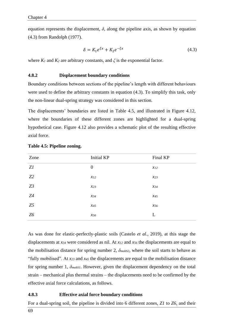
Chapter 4
69
equation represents the displacement, δ, along the pipeline axis, as shown by equation
(4.3) from Randolph (1977).
𝛿 = 𝐾1𝑒𝜉𝑥 + 𝐾2𝑒
−𝜉𝑥 (4.3)
where K1 and K2 are arbitrary constants, and ξ is the exponential factor.
4.8.2 Displacement boundary conditions
Boundary conditions between sections of the pipeline’s length with different behaviours
were used to define the arbitrary constants in equation (4.3). To simplify this task, only
the non-linear dual-spring strategy was considered in this section.
The displacements’ boundaries are listed in Table 4.5, and illustrated in Figure 4.12,
where the boundaries of these different zones are highlighted for a dual-spring
hypothetical case. Figure 4.12 also provides a schematic plot of the resulting effective
axial force.
Table 4.5: Pipeline zoning.
Zone Initial KP Final KP
Z1 0 x12
Z2 x12 x23
Z3 x23 x34
Z4 x34 x45
Z5 x45 x56
Z6 x56 L
As was done for elastic-perfectly-plastic soils (Castelo et al., 2019), at this stage the
displacements at x34 were considered as nil. At x12 and x56 the displacements are equal to
the mobilisation distance for spring number 2, δmobS2, where the soil starts to behave as
“fully mobilised”. At x23 and x45 the displacements are equal to the mobilisation distance
for spring number 1, δmobS1. However, given the displacement dependency on the total
strain – mechanical plus thermal strains – the displacements need to be confirmed by the
effective axial force calculations, as follows.
4.8.3 Effective axial force boundary conditions
For a dual-spring soil, the pipeline is divided into 6 different zones, Z1 to Z6, and their

Non-linear elastic-plastic soils
70
boundaries are provided in Table 4.5.
Zones Z1 and Z6, where the soil response is fully mobilised, are equivalent to the rigid
plastic solution with straight line behaviour and constant slopes – equations (4.4) and
(4.5):
(𝑑𝐹
𝑑𝑥)𝑍1= 𝑊(μcos 𝛽 + sin 𝛽) (4.4)
(𝑑𝐹
𝑑𝑥)𝑍6= 𝑊(μcos 𝛽 − sin 𝛽)
(4.5)
where W stands for the pipeline operational submerged weight, β for the seabed slope, μ
for the seabed friction coefficient and dF/dx for the force derivative in terms of the x
coordinate.
Zones Z2, Z3, Z4, and Z5 are the central zones. Their behaviour creates four different
parabolic curves, whose slopes vary from zero up to the values given by equations (4.4)
and (4.5).
As for Castelo et al. (2019) and as shown by Figure 4.12, the continuity of slope and
value around the five physical boundaries must be maintained. When these effective axial
force limiting conditions are rewritten, to better align with the prescriptions of the
displacement boundary conditions, the following general equations are generated for each
of the zones:
(𝑑𝐹
𝑑𝑥)𝑍1= [
𝐹𝑆1𝐹𝑇𝑜𝑡𝑎𝑙
] [−𝑊(𝜇 𝑐𝑜𝑠 𝛽 − 𝑠𝑖𝑛 𝛽)]
+ [𝐹𝑆2𝐹𝑇𝑜𝑡𝑎𝑙
] [−𝑊(𝜇 𝑐𝑜𝑠 𝛽 − 𝑠𝑖𝑛 𝛽)], 𝛿𝑥 ≤ −(𝛿𝑚𝑜𝑏𝑆2)
(𝑑𝐹
𝑑𝑥)𝑍2= [
𝐹𝑆1𝐹𝑇𝑜𝑡𝑎𝑙
] [−𝑊(𝜇 𝑐𝑜𝑠 𝛽 − 𝑠𝑖𝑛 𝛽)]
− [𝐹𝑆2𝐹𝑇𝑜𝑡𝑎𝑙
] [𝛿𝑥
(𝛿𝑚𝑜𝑏𝑆2)] [−𝑊(𝜇 𝑐𝑜𝑠 𝛽 − 𝑠𝑖𝑛 𝛽)],
−(𝛿𝑚𝑜𝑏𝑆2) < 𝛿𝑥 ≤ −(𝛿𝑚𝑜𝑏𝑆1)
(𝑑𝐹
𝑑𝑥)𝑍3= −[
𝐹𝑆1𝐹𝑇𝑜𝑡𝑎𝑙
] [𝛿𝑥
(𝛿𝑚𝑜𝑏𝑆1)] [−𝑊(𝜇 𝑐𝑜𝑠 𝛽 − 𝑠𝑖𝑛 𝛽)]
− [𝐹𝑆2𝐹𝑇𝑜𝑡𝑎𝑙
] [𝛿𝑥
(𝛿𝑚𝑜𝑏𝑆2)] [−𝑊(𝜇 𝑐𝑜𝑠 𝛽 − 𝑠𝑖𝑛 𝛽)],
−(𝛿𝑚𝑜𝑏𝑆1) < 𝛿𝑥 < 0
(4.6)
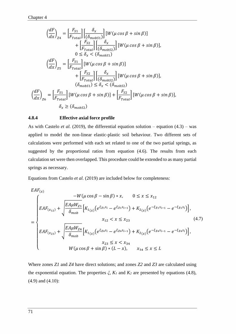
Chapter 4
71
(𝑑𝐹
𝑑𝑥)𝑍4= [
𝐹𝑆1𝐹𝑇𝑜𝑡𝑎𝑙
] [𝛿𝑥
(𝛿𝑚𝑜𝑏𝑆1)] [𝑊(𝜇 𝑐𝑜𝑠 𝛽 + 𝑠𝑖𝑛 𝛽)]
+ [𝐹𝑆2𝐹𝑇𝑜𝑡𝑎𝑙
] [𝛿𝑥
(𝛿𝑚𝑜𝑏𝑆2)] [𝑊(𝜇 𝑐𝑜𝑠 𝛽 + 𝑠𝑖𝑛 𝛽)],
0 ≤ 𝛿𝑥 < (𝛿𝑚𝑜𝑏𝑆1)
(𝑑𝐹
𝑑𝑥)𝑍5= [
𝐹𝑆1𝐹𝑇𝑜𝑡𝑎𝑙
] [𝑊(𝜇 𝑐𝑜𝑠 𝛽 + 𝑠𝑖𝑛 𝛽)]
+ [𝐹𝑆2𝐹𝑇𝑜𝑡𝑎𝑙
] [𝛿𝑥
(𝛿𝑚𝑜𝑏𝑆2)] [𝑊(𝜇 𝑐𝑜𝑠 𝛽 + 𝑠𝑖𝑛 𝛽)],
(𝛿𝑚𝑜𝑏𝑆1) ≤ 𝛿𝑥 < (𝛿𝑚𝑜𝑏𝑆2)
(𝑑𝐹
𝑑𝑥)𝑍6= [
𝐹𝑆1𝐹𝑇𝑜𝑡𝑎𝑙
] [𝑊(𝜇 𝑐𝑜𝑠 𝛽 + 𝑠𝑖𝑛 𝛽)] + [𝐹𝑆2𝐹𝑇𝑜𝑡𝑎𝑙
] [𝑊(𝜇 𝑐𝑜𝑠 𝛽 + 𝑠𝑖𝑛 𝛽)],
𝛿𝑥 ≥ (𝛿𝑚𝑜𝑏𝑆2)
4.8.4 Effective axial force profile
As with Castelo et al. (2019), the differential equation solution – equation (4.3) – was
applied to model the non-linear elastic-plastic soil behaviour. Two different sets of
calculations were performed with each set related to one of the two partial springs, as
suggested by the proportional ratios from equation (4.6). The results from each
calculation set were then overlapped. This procedure could be extended to as many partial
springs as necessary.
Equations from Castelo et al. (2019) are included below for completeness:
𝐸𝐴𝐹(𝑥)
=
{
−𝑊(𝜇 cos 𝛽 − sin 𝛽) ∗ 𝑥, 0 ≤ 𝑥 ≤ 𝑥12
𝐸𝐴𝐹(𝑥12) +√𝐸𝐴𝜇𝑊𝑍1
𝛿𝑚𝑜𝑏[𝐾1(𝑥)(𝑒
𝜉𝑍1𝑠𝑖 − 𝑒𝜉𝑍1𝑠𝑖−1) + 𝐾2(𝑥)(𝑒−𝜉𝑍1𝑠𝑖−1 − 𝑒−𝜉𝑍1𝑠𝑖)] ,
𝑥12 < 𝑥 ≤ 𝑥23
𝐸𝐴𝐹(𝑥23) +√𝐸𝐴𝜇𝑊𝑍4
𝛿𝑚𝑜𝑏[𝐾1(𝑥)(𝑒
𝜉𝑍4𝑠𝑖 − 𝑒𝜉𝑍4𝑠𝑖−1) + 𝐾2(𝑥)(𝑒−𝜉𝑍4𝑠𝑖−1 − 𝑒−𝜉𝑍4𝑠𝑖)] ,
𝑥23 ≤ 𝑥 < 𝑥34𝑊(𝜇 cos 𝛽 + sin 𝛽) ∗ (𝐿 − 𝑥), 𝑥34 ≤ 𝑥 ≤ 𝐿
(4.7)
Where zones Z1 and Z4 have direct solutions; and zones Z2 and Z3 are calculated using
the exponential equation. The properties ξ, K1 and K2 are presented by equations (4.8),
(4.9) and (4.10):

Non-linear elastic-plastic soils
72
𝜉𝑍_ =
{
𝑍1,√(
𝜇𝑊𝑍1
𝐸𝐴𝑠 ∗ 𝛿𝑚𝑜𝑏)
𝑍4,√(𝜇𝑊𝑍4
𝐸𝐴𝑠 ∗ 𝛿𝑚𝑜𝑏)
(4.8)
𝐾1𝑍_ =
{
𝑍1,
1
2√𝐸𝐴𝑠 ∗ 𝛿𝑚𝑜𝑏𝜇𝑊𝑍1
휀𝑇𝑜𝑡𝑎𝑙
𝑍4,1
2√𝐸𝐴𝑠 ∗ 𝛿𝑚𝑜𝑏𝜇𝑊𝑍4
휀𝑇𝑜𝑡𝑎𝑙
(4.9)
𝐾2𝑍_ =
{
𝑍1,−
1
2√𝐸𝐴𝑠 ∗ 𝛿𝑚𝑜𝑏𝜇𝑊𝑍1
휀𝑇𝑜𝑡𝑎𝑙
𝑍4, −1
2√𝐸𝐴𝑠 ∗ 𝛿𝑚𝑜𝑏𝜇𝑊𝑍4
휀𝑇𝑜𝑡𝑎𝑙
(4.10)
The six zones shown in equation (4.6) represent the intersection of four partial zones as
follows:
𝑍1𝐷𝑢𝑎𝑙𝑆𝑝𝑟𝑖𝑛𝑔 = 𝑍1𝑆1 + 𝑍1𝑆2
𝑍2𝐷𝑢𝑎𝑙𝑆𝑝𝑟𝑖𝑛𝑔 = 𝑍1𝑆1 + 𝑍2𝑆2
𝑍3𝐷𝑢𝑎𝑙𝑆𝑝𝑟𝑖𝑛𝑔 = 𝑍2𝑆1 + 𝑍2𝑆2
𝑍4𝐷𝑢𝑎𝑙𝑆𝑝𝑟𝑖𝑛𝑔 = 𝑍3𝑆1 + 𝑍3𝑆2
𝑍5𝐷𝑢𝑎𝑙𝑆𝑝𝑟𝑖𝑛𝑔 = 𝑍4𝑆1 + 𝑍3𝑆2
𝑍6𝐷𝑢𝑎𝑙𝑆𝑝𝑟𝑖𝑛𝑔 = 𝑍4𝑆1 + 𝑍4𝑆2
(4.11)
Now, with the effective axial force profile defined, the effective axial force variation over
the distance between stationary points, or ΔSS can be described as the summation of areas,
as given by equation (4.12), and shown in Figure 4.13.
∫ (∆𝑆𝑠)𝑑𝑥𝑆𝑃𝑆𝑈𝑝
𝑆𝑃𝑆𝐷𝑜𝑤𝑛
= −(∑|𝐴𝑟𝑒𝑎𝑖|
6
𝑖=1
) (4.12)
where each area represents the partial integral of the effective axial force in terms of the
x coordinate which takes into account the physical boundaries.
4.8.5 Analytical solution for walking rate
Similar to the revised solution for the walking rate for elastic-perfectly-plastic soils,

Chapter 4
73
WREP, in Castelo et al. (2019), the walking rate for non-linear elastic-plastic soils,
WRNLEP, can be revised to:
𝑊𝑅𝑁𝐿𝐸𝑃 = −1
𝐸𝐴(∫ (∆𝑃)𝑑𝑥
𝑆𝑃𝑆𝑈𝑝,𝑁𝐿𝐸𝑃
𝑆𝑃𝑆𝐷𝑜𝑤𝑛,𝑁𝐿𝐸𝑃
−∫ (∆𝑆𝑠)𝑑𝑥𝑆𝑃𝑆𝑈𝑝,𝑁𝐿𝐸𝑃
𝑆𝑃𝑆𝐷𝑜𝑤𝑛,𝑁𝐿𝐸𝑃
) (4.13)
where ΔP stands for the change in fully constrained force (Carr et al., 2003).
While the form of the expressions are similar for non-linear elastic-plastic and elastic-
perfectly-plastic soils, the integral limits and ΔSS expression are different, which explains
the difference and leads to more accurate results.
4.9 REVISED SOLUTION FOR THE DISTANCE BETWEEN
STATIONARY POINTS FOR NON-LINEAR ELASTIC-PLASTIC
SOIL - XAB,NLEP
As an alternative to the demanding analytical method described by section 4.8, a revised
solution may be directly obtained. From Castelo et al. (2019) where the soil is treated as
a single elastic-perfectly-plastic spring, it is known that:
𝑋𝑎𝑏,𝐸𝑃 = 𝑋𝑎𝑏,𝑅𝑃 (1 −𝛿𝑚𝑜𝑏𝛿𝑛𝑢𝑙𝑙
) (4.14)
where δnull is the non-walking mobilisation distance, as per Castelo et al. (2019), and can
be obtained by:
𝛿𝑛𝑢𝑙𝑙 =𝑊𝑅𝑅𝑃2
(4.15)
However, in this paper, the soil is treated as the combination of two or more elastic-plastic
springs. Under these conditions, equation (4.14) becomes:
𝑋𝑎𝑏,𝑁𝐿𝐸𝑃 = 𝑋𝑎𝑏,𝑅𝑃 (1 −𝛿𝑚𝑜𝑏𝐸𝑄𝛿𝑛𝑢𝑙𝑙
) (4.16)
where δmob is substituted with an equivalent mobilisation distance, δmobEQ.
4.10 REVISED SOLUTION FOR WALKING RATE FOR NON-
LINEAR ELASTIC-PLASTIC SOIL – WRNLEP
Replicating the Xab solutions, from Section 4.9, the non-linear elastic-plastic walking rate

Non-linear elastic-plastic soils
74
can be obtained from:
𝑊𝑅𝑁𝐿𝐸𝑃 = 𝑊𝑅𝑅𝑃 (1 −𝛿𝑚𝑜𝑏𝐸𝑄𝛿𝑛𝑢𝑙𝑙
) (4.17)
where δnull is the non-walking mobilisation distance, given in equation (4.15).
Equation (4.17) might be rearranged into:
𝑊𝑅𝑁𝐿𝐸𝑃 = 𝑊𝑅𝑅𝑃 − 2𝛿𝑚𝑜𝑏𝐸𝑄 (4.18)
which is an analogous solution to the solution given by Castelo et al. (2019), shown here
as equation (4.1).
4.11 EQUIVALENT MOBILISATION DISTANCE – δmobEQ
The elastic correction can be obtained by doubling the division of the unload-reload area,
AUnload-Reload, by the variation of the plastic force. These properties are shown in Figure
4.3 and the referred ratio can be calculated using equation (4.19):
𝐶𝑜𝑟𝑟𝐸𝑃 = 2( 𝐴𝑈𝑛𝑙𝑜𝑎𝑑−𝑅𝑒𝑙𝑜𝑎𝑑
𝛥𝐹𝑅) (4.19)
Following the same principles, the equivalent mobilisation distance can be acquired with
a similar procedure, as defined by equation (4.20):
𝛿𝑚𝑜𝑏𝐸𝑄 =𝐶𝑜𝑟𝑟𝑁𝐿𝐸𝑃
2= (
𝐴𝑈𝑛𝑙𝑜𝑎𝑑−𝑅𝑒𝑙𝑜𝑎𝑑𝛥𝐹𝑅
) (4.20)
4.12 FINITE ELEMENT ANALYSES PARAMETRIC STUDY
FOR DUAL-SPRING STRATEGY
The following parametric study validates the above solutions for effective axial force and
stationary points’ locations as well as walking rate for a non-linear elastic-plastic soil
using a dual-spring strategy.
The parametric study uses the values provided in Table 4.1 and previously explained in
Section 4.4 but varies the seabed slope. For simplicity, the pipeline length, pipeline
submerged operational weight and friction coefficient were kept constant, although the
shape of the non-linear response up to the limiting friction was varied. Three different
slopes (1°, 2° and 3°) were used.

Chapter 4
75
Two dual-spring parameters, δmobS1 and δmobS2, were tested in various combinations as
shown in Figure 4.14. For this paper, δmobS2 equals δmob,Soft from Castelo et al. (2019). The
elastic-perfectly-plastic soil approximations “soft” and “stiff” were used as boundary
values as shown in Figure 4.14. The region bounded by these approximations was divided
in four quadrants for displacement and four quadrants for force.
To generate the cases to be considered for the parametric study, the intersection points
were defined as the mobilisation distance, δmob, combinations. A total of six different
δmobS1 and δmobS2 pairs were used in this paper as shown in Table 4.6. Three pairs presented
in Figure 4.14 (25100, 50100, and 75100) were disregarded as they represented an elastic-
perfectly-plastic soil approach, which is not the focus of this paper.
Table 4.6: Mobilisation distance, δmob, combination cases.
Force Mobilisation Distance
Stiff “25%” “50%” “75%”
“25%” I25 SOFT FIT Not Applicable Not Applicable
“50%” I50 2550 SOFT FIT Not Applicable
“75%” I75 2575 5075 SOFT FIT
“100%” STIFF FIT 25100 50100 75100
The six different mobilisation distance, δmob, combinations, three different slopes and the
five different levels of δmobS2 allowed 90 cases to be tested in the parametric experiment.
The 90 cases were modelled using the dual-spring FEM solution.
4.12.1 Equivalent mobilisation distance – δmobEQ
Table 4.7 presents the equivalent mobilisation distance, δmobEQ, for each of the parametric
cases tested according to equation (4.20) and shown in Table 4.7. The repeated values
observed in Table 4.7 are a mathematical coincidence resulting from the values selected
for the cases.

Non-linear elastic-plastic soils
76
Table 4.7: Resultant equivalent mobilisation distance, δmobEQ.
Slope δmobS2/OD Cases
I25 (m) I50 (m) I75 (m) 2550 (m) 2575 (m) 5075 (m)
1°
0.100 0.027 0.021 0.015 0.027 0.021 0.027
0.150 0.040 0.032 0.023 0.040 0.032 0.040
0.200 0.053 0.042 0.031 0.053 0.042 0.053
0.333 0.089* 0.070* 0.051 0.089* 0.070* 0.089*
0.500 0.134* 0.105* 0.077* 0.134* 0.105* 0.134*
2°
0.100 0.027 0.021 0.015 0.027 0.021 0.027
0.150 0.040 0.032 0.023 0.040 0.032 0.040
0.200 0.053 0.042 0.031 0.053 0.042 0.053
0.333 0.089 0.070 0.051 0.089 0.070 0.089
0.500 0.134* 0.105 0.077 0.134* 0.105 0.134*
3°
0.100 0.027 0.021 0.015 0.027 0.021 0.027
0.150 0.040 0.032 0.023 0.040 0.032 0.040
0.200 0.053 0.042 0.031 0.053 0.042 0.053
0.333 0.089 0.070 0.051 0.089 0.070 0.089
0.500 0.134 0.105 0.077 0.134 0.105 0.134
Figure 4.15 presents the non-linear elastic correction results from the numerical solutions
(finite element models) plotted against the values calculated using equation (4.19). The
slopes of 1°, 2° and 3° are represented by square, circular and triangular markers,
respectively.
Figure 4.15 shows a very strong agreement between the non-linear elastic correction
obtained from the finite element analysis and the results calculated using the equation
proposed by this paper.
For Figure 4.15, 14 cases were disregarded from the 90 cases tested as the pipeline
* Values of equivalent mobilisation distance that are greater than the non-walking mobilisation distance, as
per Table 4.8 values (δmobEQ>δnull).
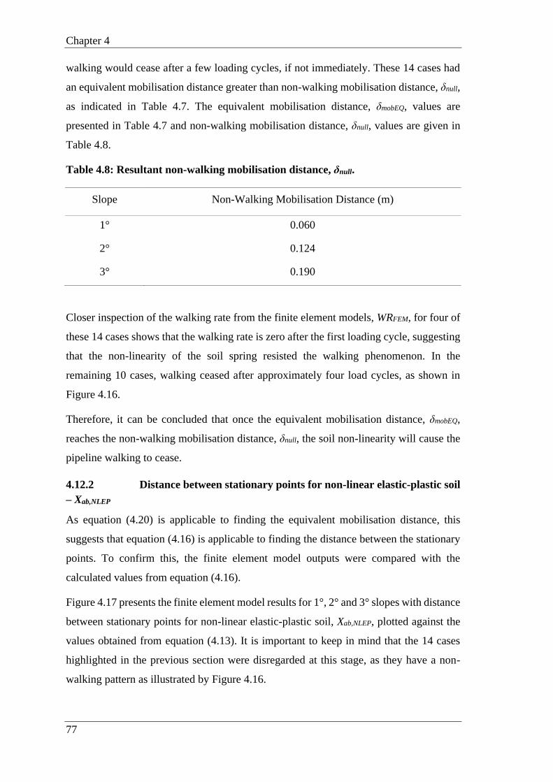
Chapter 4
77
walking would cease after a few loading cycles, if not immediately. These 14 cases had
an equivalent mobilisation distance greater than non-walking mobilisation distance, δnull,
as indicated in Table 4.7. The equivalent mobilisation distance, δmobEQ, values are
presented in Table 4.7 and non-walking mobilisation distance, δnull, values are given in
Table 4.8.
Table 4.8: Resultant non-walking mobilisation distance, δnull.
Slope Non-Walking Mobilisation Distance (m)
1° 0.060
2° 0.124
3° 0.190
Closer inspection of the walking rate from the finite element models, WRFEM, for four of
these 14 cases shows that the walking rate is zero after the first loading cycle, suggesting
that the non-linearity of the soil spring resisted the walking phenomenon. In the
remaining 10 cases, walking ceased after approximately four load cycles, as shown in
Figure 4.16.
Therefore, it can be concluded that once the equivalent mobilisation distance, δmobEQ,
reaches the non-walking mobilisation distance, δnull, the soil non-linearity will cause the
pipeline walking to cease.
4.12.2 Distance between stationary points for non-linear elastic-plastic soil
– Xab,NLEP
As equation (4.20) is applicable to finding the equivalent mobilisation distance, this
suggests that equation (4.16) is applicable to finding the distance between the stationary
points. To confirm this, the finite element model outputs were compared with the
calculated values from equation (4.16).
Figure 4.17 presents the finite element model results for 1°, 2° and 3° slopes with distance
between stationary points for non-linear elastic-plastic soil, Xab,NLEP, plotted against the
values obtained from equation (4.13). It is important to keep in mind that the 14 cases
highlighted in the previous section were disregarded at this stage, as they have a non-
walking pattern as illustrated by Figure 4.16.
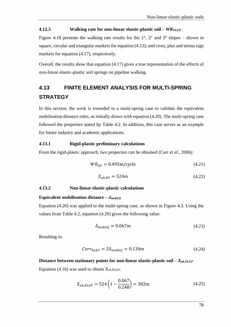
Non-linear elastic-plastic soils
78
4.12.3 Walking rate for non-linear elastic-plastic soil – WRNLEP
Figure 4.18 presents the walking rate results for the 1°, 2° and 3° slopes – shown in
square, circular and triangular markers for equation (4.13); and cross, plus and minus sign
markers for equation (4.17), respectively.
Overall, the results show that equation (4.17) gives a true representation of the effects of
non-linear elastic-plastic soil springs on pipeline walking.
4.13 FINITE ELEMENT ANALYSIS FOR MULTI-SPRING
STRATEGY
In this section, the work is extended to a multi-spring case to validate the equivalent
mobilisation distance rules, as initially drawn with equation (4.20). The multi-spring case
followed the properties stated by Table 4.2. In addition, this case serves as an example
for future industry and academic applications.
4.13.1 Rigid-plastic preliminary calculations
From the rigid-plastic approach, two properties can be obtained (Carr et al., 2006):
𝑊𝑅𝑅𝑃 = 0.495m/cycle (4.21)
𝑋𝑎𝑏,𝑅𝑃 = 524m (4.22)
4.13.2 Non-linear elastic-plastic calculations
Equivalent mobilisation distance – δmobEQ
Equation (4.20) was applied to the multi-spring case, as shown in Figure 4.3. Using the
values from Table 4.2, equation (4.20) gives the following value:
𝛿𝑚𝑜𝑏𝐸𝑄 = 0.067m (4.23)
Resulting in:
𝐶𝑜𝑟𝑟𝑁𝐿𝐸𝑃 = 2𝛿𝑚𝑜𝑏𝐸𝑄 = 0.134m (4.24)
Distance between stationary points for non-linear elastic-plastic soil – Xab,NLEP
Equation (4.16) was used to obtain Xab,NLEP:
𝑋𝑎𝑏,𝑁𝐿𝐸𝑃 = 524 (1 −0.067
0.248) = 382m (4.25)

Chapter 4
79
Walking rate for non-linear elastic-plastic soil – WRNLEP
Equation (4.18) was used to calculate WRNLEP:
𝑊𝑅𝑁𝐿𝐸𝑃 = 0.495 − 0.134 = 0.361m/cycle (4.26)
4.13.3 Non-linear elastic-plastic finite element model results
Distance between stationary points from finite element analysis – Xab,FEM
From the finite element analysis, the obtained Xab value was:
𝑋𝑎𝑏𝐹𝐸𝑀 = 380m (4.27)
Walking rate from finite element analysis – WRFEM
From the finite element model, the obtained walking rate value was:
𝑊𝑅𝐹𝐸𝑀 = 0.359m/cycle (4.28)
Overall, the outcome for the finite element model multi-spring strategy shows a very
good agreement with the proposed analytical methods and demonstrates that they can be
used for modelling more complex forms of non-linearity of elastic-plastic soils, resulting
in a very small deviation.
4.14 CONCLUSIONS & FINAL REMARKS
This paper provides a new strategy to solve downslope pipeline walking problems
considering non-linear elastic-plastic soil representations. Different shapes and properties
of non-linearity (within the elastic-plastic range) have been considered leading to an
innovative analytical solution. This new solution improves understanding of the main
properties involved in the non-linear elastic-plastic soil behaviour by providing a set of
analytical expressions for pipe walking, which were benchmarked and validated against
a set of finite element analyses.
Current solutions do not consider the non-linearity of soil response, and this idealisation
is known to affect the resulting walking pattern. It is also difficult to specify a suitable
elastic stiffness when the soil response observed in model tests is strongly non-linear.
Therefore, this paper resolves how the fundamental solution must be adjusted to allow
for non-linear elastic-plastic soils.
Finally, the paper presents how the non-linear elastic-plastic problem might be translated
into an elastic-perfectly-plastic soil spring by using the equivalent mobilisation distance,

Non-linear elastic-plastic soils
80
δmobEQ. This very simple and direct solution provides an accurate estimate of the walking
rate of offshore pipelines in a non-linear soil and avoids numerical modelling which can
be time- and resource-consuming.

Chapter 4
81
FIGURES
Figure 4.1: Effective axial force diagrams for start-up and shutdown phases.
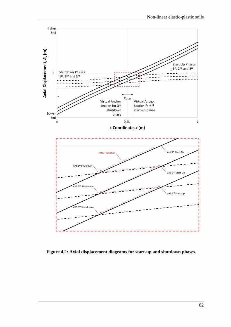
Non-linear elastic-plastic soils
82
Figure 4.2: Axial displacement diagrams for start-up and shutdown phases.
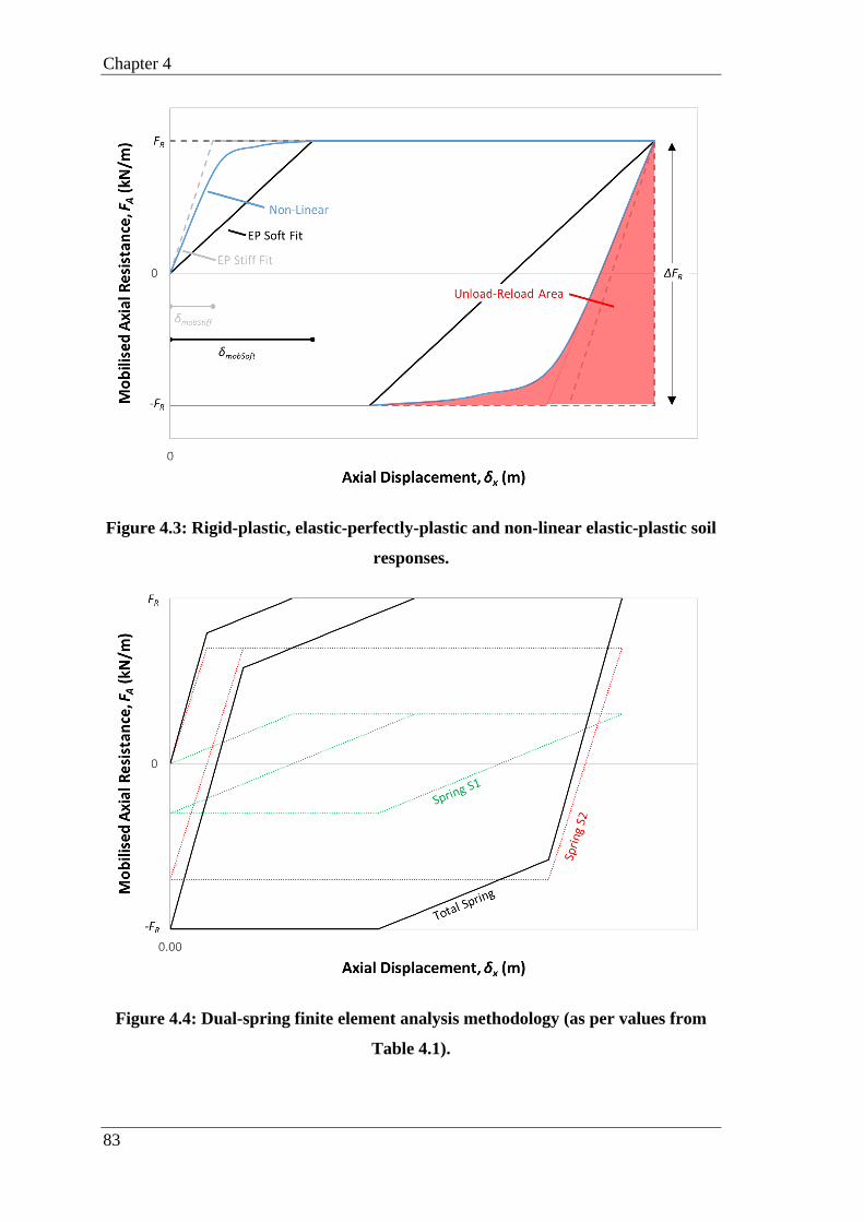
Chapter 4
83
Figure 4.3: Rigid-plastic, elastic-perfectly-plastic and non-linear elastic-plastic soil
responses.
Figure 4.4: Dual-spring finite element analysis methodology (as per values from
Table 4.1).
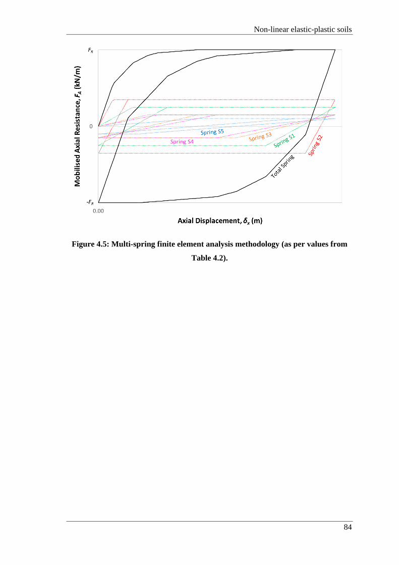
Non-linear elastic-plastic soils
84
Figure 4.5: Multi-spring finite element analysis methodology (as per values from
Table 4.2).
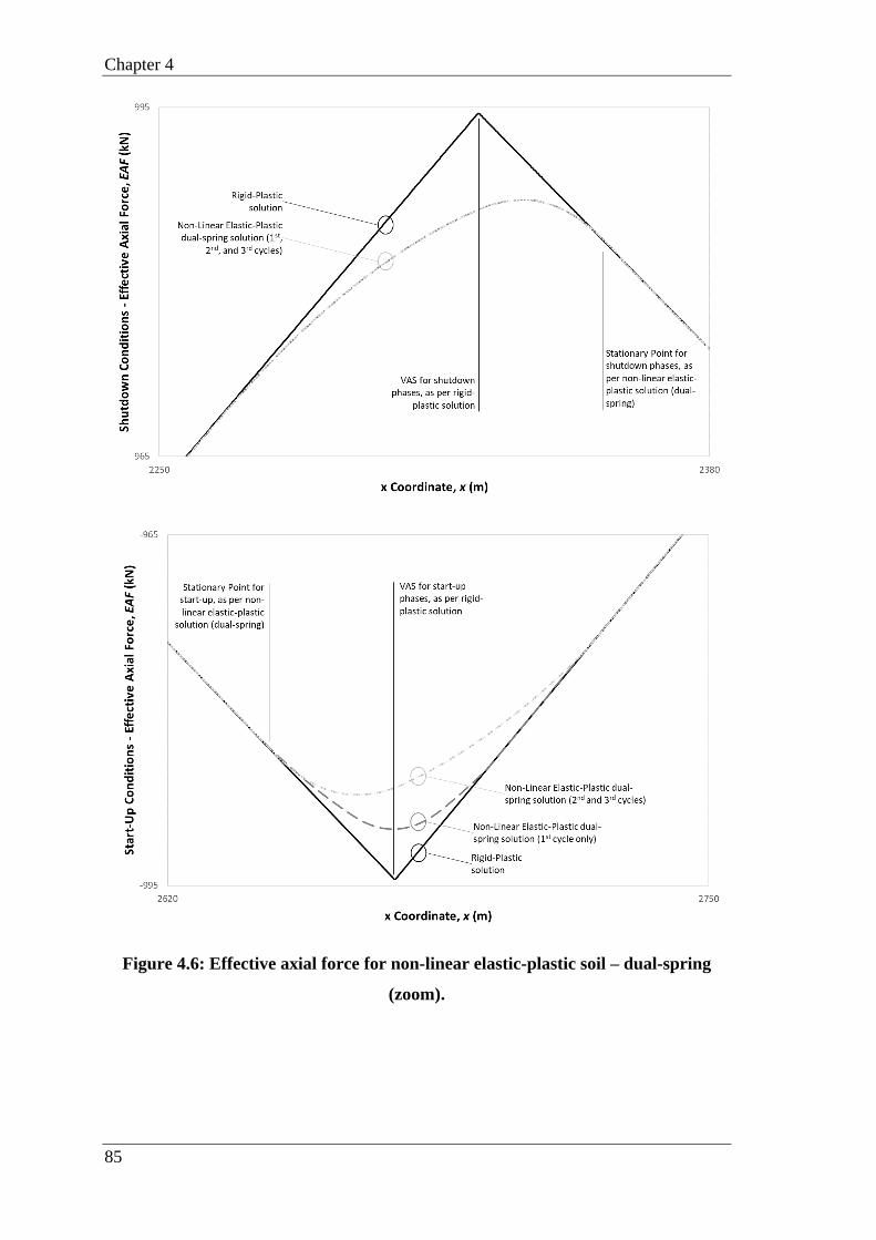
Chapter 4
85
Figure 4.6: Effective axial force for non-linear elastic-plastic soil – dual-spring
(zoom).
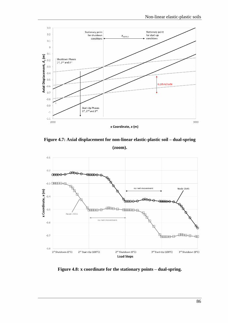
Non-linear elastic-plastic soils
86
Figure 4.7: Axial displacement for non-linear elastic-plastic soil – dual-spring
(zoom).
Figure 4.8: x coordinate for the stationary points – dual-spring.

Chapter 4
87
Figure 4.9: Effective axial force for non-linear elastic-plastic soil – multi-spring
(zoom).

Non-linear elastic-plastic soils
88
Figure 4.10: Axial displacement for non-linear elastic-plastic soil – multi-spring
(zoom).
Figure 4.11: x coordinate for the stationary points – multi-spring.

Chapter 4
89
Figure 4.12: Schematic plot accounting physical boundaries.
Figure 4.13: Schematic plot accounting physical boundaries.

Non-linear elastic-plastic soils
90
Figure 4.14: Mobilisation distance, δmob, combination spectrum.
Figure 4.15: Non-linear elastic correction results.

Chapter 4
91
Figure 4.16: Walking rate from finite element models, WRFEM, results for selected
cases.
Figure 4.17: Distance between stationary points results.

Non-linear elastic-plastic soils
92
Figure 4.18: Walking rate results.
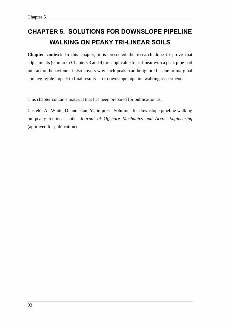
Chapter 5
93
CHAPTER 5. SOLUTIONS FOR DOWNSLOPE PIPELINE
WALKING ON PEAKY TRI-LINEAR SOILS
Chapter context: In this chapter, it is presented the research done to prove that
adjustments (similar to Chapters 3 and 4) are applicable to tri-linear with a peak pipe-soil
interaction behaviour. It also covers why such peaks can be ignored – due to marginal
and negligible impact to final results – for downslope pipeline walking assessments.
This chapter contains material that has been prepared for publication as:
Castelo, A., White, D. and Tian, Y., in press. Solutions for downslope pipeline walking
on peaky tri-linear soils. Journal of Offshore Mechanics and Arctic Engineering
(approved for publication)

Tri-linear soils with a peak
94
5.1 ABSTRACT
Offshore pipelines used for transporting hydrocarbons are cyclically loaded by great
variations of pressure and temperature. These variations can induce axial instability in
such pipelines. This instability may cause the pipelines to migrate globally along their
length; an effect known as pipeline walking. Traditional models of pipeline walking have
considered the axial soil response as rigid-plastic; however, such behaviour does not
match observations from physical soil tests. It leads to poor estimates of walking rate per
cycle and over design. In this paper, the impact of a tri-linear (3L) soil idealization
accounting for a peak break-out behaviour on pipeline walking is investigated. Different
shapes and properties of tri-linearity (within the peaky soil range) have been considered
leading to an innovative analytical solution. The new solution improves understanding of
the main properties involved in the peaky tri-linear soil behaviour by providing a set of
analytical expressions for pipe walking, which were benchmarked and validated against
a set of finite element analyses.
5.2 INTRODUCTION
As the hydrocarbon industry increasingly explores deep water reservoirs, offshore
pipelines become progressively important. When these pipelines are exposed to
operational load cycles, they expand and contract in response to temperature and pressure
changes. However, these expansion and contraction cycles may have an asymmetric
behaviour due to seabed slopes or other factors, such as multiphasic flow (Bruton et al.,
2010), and thermal transients (Carr et al., 2006). The asymmetric expansion and
contraction directly impacts the stability of these pipelines causing them to migrate in
one direction, which generates the phenomenon known as pipeline walking (Carr et al.,
2003). Pipeline walking increases cost and risk and may severely impact the subsea
system (Tornes et al., 2000). It may overstress connections, alter loads and strains in any
engineered lateral buckle and may also present the need for anchoring. Hence, accurately
identifying and estimating pipeline walking is necessary to decrease the risk of
production loss and environmental damage, and it can significantly decrease project
development costs.
Presently, the common practice in the industry is to evaluate pipeline walking during the
design phase using a set of analytical formulations as per Bruton et al. (2010). These
calculations consider various aspects, such as operational (temperature, pressure, etc.),
Chapter 5
95
environmental (seabed overall slope angle, soil friction coefficient, etc.) and physical
pipeline properties (length, steel wall thickness, etc.). Accurately evaluating high-
temperature and high-pressure pipelines for downslope pipeline walking is of paramount
importance to the industry because these conditions are commonly found in fully
operational areas, such as the Gulf of Mexico, North Sea and Northwest Australia, as well
as in frontier locations, which are still in early stages of exploration, such as the Brazilian
Pre-Salt and the Arctic Region. The analytical formulation is idealised and can provide
inaccurate walking rates. Then, the assessment requires further analyses to overcome the
aforementioned limitations.
Costly and time-demanding finite element analyses are used to confirm walking
behaviour and to generate a reliable walking rate. However, emerging academic research
(Castelo et al., 2019, in press b) demonstrates that, if the adequate soil behaviour is
considered in the initial analytical formulae, the requirement for time demanding and
expensive analyses can be reduced.
Although the formulation developed by Castelo et al. (2019, in press b) generate
significant cost-savings and improve efficiency, they are limited to a single soil range,
i.e. elastic-plastic (elastic-perfectly-plastic and non-linear elastic-plastic, respectively).
Therefore, further improvement is needed to capture the walking behaviour with soils
that develop a peak breakout resistance before reaching a plastic plateau, as commonly
seen in the operational areas mentioned above, and thus the accuracy of pipeline walking
results for analytical formulae is increased.
This paper investigates the impact on pipeline walking of a tri-linear soil idealization
accounting for a peak break-out behaviour. It starts by a brief literature review of the
present methodology used to estimate the walking rate for elastic-plastic soils (Castelo et
al., 2019, in press b). It then builds on the previous knowledge to generate theoretical
expressions for pipeline walking on peaky tri-linear soils. Next, finite element analyses
are performed to provide confirmation of the theoretical framework. Finally, this paper
generates a solution that allows an adjustment for the original rigid-plastic analytical
formulation (Bruton et al., 2010), so that the requirement for finite element analyses can
be reduced.

Tri-linear soils with a peak
96
5.3 BACKGROUND TO PIPELINE WALKING
5.3.1 Downslope mechanism
The seabed slope generates an asymmetry between the start-up and shutdown phases in
the effective axial force profile for a fully mobilised pipeline, as illustrated in Figure 5.1,
where the rigid-plastic soil condition is considered. This asymmetry causes the virtual
anchor sections to be separated by a given distance, Xab. For rigid-plastic soil
representations, the virtual anchor sections correspond to the maximum absolute effective
axial force along the pipeline length. Then, the distance Xab can be associated to the axial
displacement, δx, from a particular load phase (start-up and shutdown phases), as
presented by Figure 5.2. Because it tends to create unbalanced displacements during
different loading stages, the asymmetry in the effective axial force profile is presently
understood to be the root cause of pipeline walking.
Accounting for more realistic soil conditions, the distance Xab cannot be associated with
maximum effective axial force. Therefore, Xab must be associated with the stationary
points, as thoroughly explained in Castelo et al. (2019).
5.3.2 Pipe-soil response
Previous research on pipeline walking has treated soils as rigid-plastic (Carr et al., 2003;
2006; Bruton et al., 2010) or as elastic-plastic (Castelo et al., 2019, in press b). However,
it is known that some soils behave differently, producing first a breakout peak resistance
and then decreasing their resistance to a residual plastic level.
Although many other studies, such as White et al. (2011), have already investigated
peaky soils in general terms, none has gone through the specific impact of these soils on
pipeline walking. This paper focuses on a soil representation that accounts for breakout
soil resistance using a peaky tri-linear (3L) soil representation and how pipeline walking
may change due to this different soil condition.
5.4 PROBLEM DEFINITION
Downslope pipeline walking is dependent on three types of properties: environmental,
operational and those of the pipeline. This paper’s parametric study uses typical
parameter ranges for these three properties.
The environmental parameters include seabed slope angle and residual friction
coefficient, taken to be 2ᵒ and 0.25, respectively. The operational parameters include

Chapter 5
97
temperature variation and pipe submerged weight, assumed to be 100°C and 0.4kN/m,
respectively. The physical pipeline properties include steel outside diameter, steel wall
thickness and length, taken to be 0.3239m, 0.0206m and 5000m, respectively. Some
additional environmental properties were taken as variables for the parametric study, and
they are related to the pipe-soil response (cases i - iv). The full list of properties and
parameters used in this study are provided in Table 5.1 and Table 5.2.
Table 5.1: General properties.
Parameter Value
Steel outside diameter, OD 0.3239m
Steel wall thickness, t 0.0206m
Length, L 5000m
Seabed slope angle, β 2.0°
Temperature variation, ΔT 100°C
Pipe submerged weight, W 0.4kN/m
Residual friction coefficient, μ 0.25
Steel Young's modulus, E 2.07x10¹¹Pa
Steel Poisson coefficient, ν 0.3
Steel thermal expansion coefficient, α 1.165x10⁻⁵°C-1
Table 5.2: Case properties.
Property Cases
i ii iii iv
Peak Elastic Force, FP (kN) 0.200 0.400 0.300 0.250
Peak Elastic Force Mobilisation distance,
δmobP (m) 0.129 0.129 0.129 0.129
Residual Plastic Force, FR (kN) 0.100 0.100 0.100 0.100
Residual Plastic Force Mobilisation distance,
δmobR (m) 0.162 0.162 0.162 0.162
Ideal Mobilisation distance, δmob’ (m) 0.065 0.032 0.043 0.052

Tri-linear soils with a peak
98
Figure 5.3 presents a schematic axial force-displacement response for an ideal set of
peaky tri-linear soil cases. As investigated in White et al. (2011), it is known that various
aspects affect the cyclic behaviour of peaky soils. These aspects may be related, but not
limited, to the time interval between distinct movements, the varying pipeline
embedment, etc. As a result, this paper takes into account two different extreme
conditions:
• “EqualPeaks”;
• “NoSUpPeak”.
As the conditions’ names suggest, the first condition, “EqualPeaks”, behaves with equal
peaks for both loading phases – start-up and shutdown. Alternatively, the second
condition, “NoSUpPeak”, behaves with no peak for start-up phases, while peaky for
shutdown phases. There is no clear understanding in the literature as to why the peak
dissipation may occur for one load phase, while it may not occur for another load phase.
Consequently, the axial force-displacement responses, shown in Figure 5.3, need to be
updated to account for cyclic movements. Figure 5.4 shows the update to Figure 5.3,
presenting three hypothetical load steps for “EqualPeaks” and “NoSUpPeak” conditions.
Although the authors acknowledge that intermediate peak cases may occur in between
“EqualPeaks” and “NoSUpPeak” conditions, these intermediate conditions would be
enveloped by these two extreme conditions. For this reason, the intermediate cases are
disregarded in this paper. For simplicity, it is also assumed that the first load phase does
not peak.
5.5 ELASTIC-PERFECTLY-PLASTIC SOLUTION FOR
PIPELINE WALKING
From Castelo et al. (in press b) it is known that the walking rate for an elastic-plastic
pipe-soil response, WREP, can be obtained simply by subtracting twice the equivalent
mobilisation distance, δmobEQ, from the walking rate for rigid-plastic soil, WRRP, as shown
by equation (5.1):
𝑊𝑅𝐸𝑃 = 𝑊𝑅𝑅𝑃 − 2 ∗ 𝛿𝑚𝑜𝑏𝐸𝑄 (5.1)
where the walking rate for rigid-plastic soil can be estimated from Carr et al. (2006) and
the equivalent mobilisation distance for a non-linear elastic-plastic pipe-soil response can
be obtained from Castelo et al. (in press b).

Chapter 5
99
As another option, reorganizing equation (5.1), as also explained by Castelo et al. (in
press b), the walking rate for an elastic-plastic pipe-soil response can be established by
multiplying the walking rate for rigid-plastic soil by a reduction factor based on the
equivalent mobilisation distance and the non-walking mobilisation distance, δnull, as
presented by equation (5.2):
𝑊𝑅𝐸𝑃 = 𝑊𝑅𝑅𝑃 ∗ (1 −𝛿𝑚𝑜𝑏𝐸𝑄𝛿𝑛𝑢𝑙𝑙
) (5.2)
where the non-walking mobilisation distance, δnull, can be achieved using equation (5.3)
– (Castelo et al., 2019):
𝛿𝑛𝑢𝑙𝑙 =𝑊𝑅𝑅𝑃2
(5.3)
As confirmed by Castelo et al. (in press b), the same reduction factor can be applied to
the distance between stationary points for an elastic-plastic pipe-soil response, Xab,EP, as
presented below by equation (5.4):
𝑋𝑎𝑏,𝐸𝑃 = 𝑋𝑎𝑏,𝑅𝑃 ∗ (1 −𝛿𝑚𝑜𝑏𝐸𝑄𝛿𝑛𝑢𝑙𝑙
) (5.4)
where the distance between stationary points for rigid-plastic soil, Xab,RP, can be estimated
from Bruton et al. (2010).
A parametric study has been performed using finite element analyses, to investigate the
peaky tri-linear pipe-soil responses seen in Figure 5.4, aiming on building on equation
(5.1) to create an accurate, simple and fast methodology to estimate pipeline walking for
this pipe-soil response type.
5.6 FINITE ELEMENT METHODOLOGY
The finite element model used in this paper is based on a straight pipeline laid on a
uniformly sloping seabed. The properties of this model are presented in Table 5.1 and
Table 5.2 (soil case ii). Table 5.2 also presents data used for the parametric study
developed later in this paper.
The 5000m pipeline was represented by 5001 nodes connected by 5000 equal Euler
Bernoulli beam elements (B33 – 3 dimensional 3 noded elements in Abaqus), creating a
1 metre “mesh” size.

Tri-linear soils with a peak
100
To represent the peaky tri-linear pipe-soil interaction, the soil was modelled as a set of
macro elements connected to each pipeline node, which were described as user elements
in FORTRAN.
5.6.1 Peaky tri-linear pipe-soil interaction models
Two different soil conditions were modelled for this paper: the “EqualPeaks” and
“NoSUpPeak” extreme conditions as shown in Figure 5.4.
For the “EqualPeaks” condition, the user element interface applied a constant (positive)
stiffness until a predefined peak force was attained. At this peak force a constant
(negative) stiffness was applied, so that the reaction force reduced up to a residual plateau.
If the displacement was reversed, the same behaviour could be observed for the spring-
slider in the opposite direction.
For the “NoSUpPeak” condition, the user element interface applied the same forces
during loading as applied in the “EqualPeaks” condition. However, for start-up phases,
the forces did not present the peak, because once the reaction force achieved the residual
plateau, no further reaction was provided and the applied stiffness at this point was zero,
where the forces remained in the residual plateau.
5.6.2 Loads
In the analysis, the pipeline was heated up uniformly with a temperature increase of
100°C. This value includes an additional temperature amount that represents the pipe
internal pressure (Hobbs, 1984).
The self-weight of the pipeline, W, and seabed slope angle, β, generate a sliding
component to the weight:
𝑊𝑐𝑜𝑚𝑝 = 𝑊 sin 𝛽 (5.5)
Operational cycling took into account the steady operational profile (start-up) and the rest
condition (shutdown).
5.7 FINITE ELEMENT ANALYSIS RESULTS AND
COMPARISON WITH RIGID-PLASTIC SOLUTION
Figure 5.5 and Figure 5.6 show the effective axial force and the axial displacement
distribution, respectively, for the “EqualPeaks” condition applied to ideal case ii.
Figure 5.7 and Figure 5.8 show the effective axial force and the axial displacement
Chapter 5
101
distribution for “NoSUpPeak” condition applied to ideal case ii.
Although these two finite element analyses (“EqualPeaks” and “NoSUpPeak”) provided
similar results when compared to each other, as shown in Table 5.3, when compared to
the analytical calculations from Bruton et al. (2010), as shown in Table 5.4, the deviation
presented a remarkable margin.
Table 5.3: Tri-linear finite element analysis results for soil case ii.
Case Distance Between Stationary Points Walking Rate
ii EqualPeaks 637m 0.674m/cycle
NoSUpPeak 638m 0.675m/cycle
Table 5.4: Rigid-plastic calculation results.
Case Distance Between Stationary Points Walking Rate
Rigid-plastic (Carr et al., 2006) 698m 0.740m/cycle
The deviation between rigid-plastic calculations and finite element results (61m for the
distance between stationary points and 0.066m/cycle for the walking rate) is justified by
the fact that the finite element analyses considered a more realistic soil. Instead of using
a basic soil approximation, rigid-plastic, the analyses considered a more realistic soil
response, peaky tri-linear pipe-soil interaction.
To estimate the realistic results for the distance between stationary points and for the
walking rate, a new analytical solution is outlined for the peaky tri-linear pipe-soil
response, as was done in Castelo et al. (2019, in press b).
5.8 REVISED ANALYTICAL SOLUTION FOR THE
DISTANCE BETWEEN STATIONARY POINTS FOR PEAKY TRI-
LINEAR SOILS – Xab,3L
From Castelo et al. (in press b) where the soil is treated as a non-linear elastic-plastic
spring, it is known that the distance between stationary points, Xab,EP, is equal to the
distance between stationary points for rigid-plastic soils, Xab,RP, multiplied by a reduction
factor, which is based on the equivalent mobilisation distance, δmobEQ, and the non-

Tri-linear soils with a peak
102
walking mobilisation distance, δnull, as shown by equation (5.4).
Alternatively, for a peaky tri-linear pipe-soil behaviour, the equivalent mobilisation
distance, δmobEQ, might be substituted by an ideal mobilisation distance, δmob’.
𝑋𝑎𝑏,3𝐿 = 𝑋𝑎𝑏,𝑅𝑃 ∗ (1 −𝛿𝑚𝑜𝑏′
𝛿𝑛𝑢𝑙𝑙) (5.6)
5.9 REVISED ANALYTICAL SOLUTION FOR THE
WALKING RATE FOR PEAKY TRI-LINEAR SOILS – WR3L
From Castelo et al. (in press b), which treated the soil as a non-linear elastic-plastic
spring, it is known that the walking rate, WREP, is equal to the walking rate for rigid-
plastic soils, WRRP, multiplied by a reduction factor based on the equivalent mobilisation
distance, δmobEQ, and the non-walking mobilisation distance, δnull, as previously shown by
equation (5.2).
Analogously to Xab,3L, for a peaky tri-linear pipe-soil behaviour, the equivalent
mobilisation distance, δmobEQ, might be substituted by an ideal mobilisation distance,
δmob’.
𝑊𝑅3𝐿 = 𝑊𝑅𝑅𝑃 ∗ (1 −𝛿𝑚𝑜𝑏′
𝛿𝑛𝑢𝑙𝑙) (5.7)
5.10 IDEAL MOBILISATION DISTANCE - δmob’
As firstly developed by Castelo et al. (2019) and further expanded by Castelo et al. (in
press b) for the elastic correction, the tri-linear correction, Corr3L, for the walking rate
predictions can be obtained by doubling the division of the unload-reload area, AUnload-
Reload, by the variation of residual plastic force, ΔFR. However, differently to elastic-
plastic soils, peaky tri-linear pipe-soil interactions have an additional area, created by the
peak resistance, but the influence of the peak resistance is so small, that this additional
area can be safely ignored resulting in:
𝐶𝑜𝑟𝑟3𝐿 = 2(𝐴𝑈𝑛𝑙𝑜𝑎𝑑−𝑅𝑒𝑙𝑜𝑎𝑑
𝛥𝐹𝑅) (5.8)
Then, following the same principles, the ideal mobilisation distance, δmob’, can be
described with a similar procedure from Castelo et al. (2019, in press b), as outlined by

Chapter 5
103
equation (5.9):
𝛿𝑚𝑜𝑏′ =𝐶𝑜𝑟𝑟3𝐿2
= (𝐴𝑈𝑛𝑙𝑜𝑎𝑑−𝑅𝑒𝑙𝑜𝑎𝑑
𝛥𝐹𝑅) (5.9)
As another option, since the soil behaves linearly, δmob’ can also be written as:
𝛿𝑚𝑜𝑏′ =𝐹𝑅 ∗ 𝛿𝑚𝑜𝑏𝑃
𝐹𝑃 (5.10)
where FR is the residual plastic force, FP is the peak elastic force, and δmobP is the
mobilisation distance where the peak elastic force is achieved.
Now, using the values provided in Table 2, δmob’ was calculated for cases i - iv to be
0.065, 0.032, 0.043 and 0.052m, respectively; while, equations (5.4) and (5.7) were
rewritten, accounting for equation (5.10), as:
𝑋𝑎𝑏,3𝐿 = 𝑋𝑎𝑏,𝑅𝑃 (1 −𝐹𝑅𝐹𝑃
𝛿𝑚𝑜𝑏𝑃𝛿𝑛𝑢𝑙𝑙
) (5.11)
𝑊𝑅3𝐿 = 𝑊𝑅𝑅𝑃 ∗ (1 −𝐹𝑅𝐹𝑃
𝛿𝑚𝑜𝑏𝑃𝛿𝑛𝑢𝑙𝑙
) (5.12)
Hence, using equations (5.11) and (5.12) in association to the values provided by Table
5.1, Table 5.2 and Table 5.4, the distance between stationary points and the walking rate
were obtained, as presented by Table 5.5†.
Table 5.5: Analytical results.
Case Distance Between Stationary Points Walking Rate
i 576m 0.610m/cycle
ii 637m 0.675m/cycle
iii 617m 0.653m/cycle
iv 600m 0.636m/cycle
† The authors understand that 1m lies inside the acceptable deviation given that this is the mesh spacing.
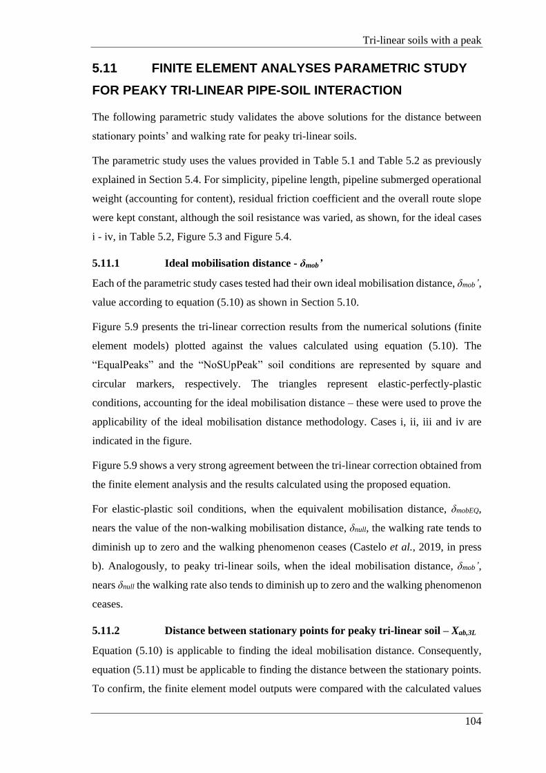
Tri-linear soils with a peak
104
5.11 FINITE ELEMENT ANALYSES PARAMETRIC STUDY
FOR PEAKY TRI-LINEAR PIPE-SOIL INTERACTION
The following parametric study validates the above solutions for the distance between
stationary points’ and walking rate for peaky tri-linear soils.
The parametric study uses the values provided in Table 5.1 and Table 5.2 as previously
explained in Section 5.4. For simplicity, pipeline length, pipeline submerged operational
weight (accounting for content), residual friction coefficient and the overall route slope
were kept constant, although the soil resistance was varied, as shown, for the ideal cases
i - iv, in Table 5.2, Figure 5.3 and Figure 5.4.
5.11.1 Ideal mobilisation distance - δmob’
Each of the parametric study cases tested had their own ideal mobilisation distance, δmob’,
value according to equation (5.10) as shown in Section 5.10.
Figure 5.9 presents the tri-linear correction results from the numerical solutions (finite
element models) plotted against the values calculated using equation (5.10). The
“EqualPeaks” and the “NoSUpPeak” soil conditions are represented by square and
circular markers, respectively. The triangles represent elastic-perfectly-plastic
conditions, accounting for the ideal mobilisation distance – these were used to prove the
applicability of the ideal mobilisation distance methodology. Cases i, ii, iii and iv are
indicated in the figure.
Figure 5.9 shows a very strong agreement between the tri-linear correction obtained from
the finite element analysis and the results calculated using the proposed equation.
For elastic-plastic soil conditions, when the equivalent mobilisation distance, δmobEQ,
nears the value of the non-walking mobilisation distance, δnull, the walking rate tends to
diminish up to zero and the walking phenomenon ceases (Castelo et al., 2019, in press
b). Analogously, to peaky tri-linear soils, when the ideal mobilisation distance, δmob’,
nears δnull the walking rate also tends to diminish up to zero and the walking phenomenon
ceases.
5.11.2 Distance between stationary points for peaky tri-linear soil – Xab,3L
Equation (5.10) is applicable to finding the ideal mobilisation distance. Consequently,
equation (5.11) must be applicable to finding the distance between the stationary points.
To confirm, the finite element model outputs were compared with the calculated values

Chapter 5
105
from equation (5.11).
Figure 5.10 presents the results for the distance between stationary points using numerical
solutions (finite element models) plotted against the values calculated using equation
(5.11). The “EqualPeaks” and the “NoSUpPeak” soil conditions are represented by
square and circular markers, respectively. The triangles represent elastic-perfectly-plastic
conditions, accounting for the ideal mobilisation distance. Cases i, ii, iii and iv are
indicated in the figure.
Figure 5.10 shows a very strong agreement for the distance between stationary points
obtained from the finite element analysis and the results calculated using the proposed
equation.
5.11.3 Walking rate for peaky tri-linear soil – WR3L
Figure 5.11 presents the walking rate results from the numerical solutions (finite element
models) plotted against the values calculated using equation (5.12). The “EqualPeaks”
and the “NoSUpPeak” soil conditions are represented by square and circular markers,
respectively. The triangles represent elastic-perfectly-plastic conditions, accounting for
the ideal mobilisation distance. Cases i, ii, iii and iv are indicated in the figure.
Figure 5.11 shows a very strong agreement between the walking rates obtained from the
finite element analysis and the results calculated using the proposed equation.
Overall, the results show that equation (5.12) – as presented by Table 5.6 – gives a true
representation of the effects of peaky tri-linear soil springs on pipeline walking.
Table 5.6: Tri-linear finite element analyses results.
Case Distance Between Stationary Points Walking Rate
i EqualPeaks 577m 0.611m/cycle
NoSUpPeak 577m 0.611m/cycle
ii EqualPeaks 637m 0.674m/cycle
NoSUpPeak 638m 0.675m/cycle
iii EqualPeaks 616m 0.652m/cycle
NoSUpPeak 617m 0.653m/cycle
iv EqualPeaks 600m 0.635m/cycle
NoSUpPeak 601m 0.636m/cycle

Tri-linear soils with a peak
106
Finally, Equation (5.1) can be translated for peaky tri-linear soils as equation (5.13):
𝑊𝑅3𝐿 = 𝑊𝑅𝑅𝑃 − 2𝛿𝑚𝑜𝑏′ (5.13)
where the walking rate for peaky tri-linear soils, WR3L, may be directly obtained by
subtracting twice the ideal mobilisation distance, δmob’, from the walking rate for rigid-
plastic soils, WRRP.
5.12 OBSERVATIONS ABOUT THE EFFECTIVE AXIAL
FORCE VARIATION OVER THE DISTANCE BETWEEN
STATIONARY POINTS FOR PEAKY TRI-LINEAR SOILS – ΔSS,3L
For Castelo et al. (2019, in press b), the effective axial force variation over the distance
between stationary points, ΔSS, solution was mathematically revised by making
adjustments for the effective axial force physical boundaries, the axial displacement, δx,
boundary conditions and the effective axial force boundary conditions. These factors
directly impact the differential equation used to obtain the effective axial force values
and ultimately change the ΔSS expression.
While obtaining the effective axial force variation over the distance between stationary
points is important, previous experience (Castelo et al., 2019, in press b), shows that ΔSS
revision will not have a significant impact on finding the walking rate for peaky tri-linear
soils. Furthermore, confidence in the numerical solutions obtained in previous research,
and the use of similar approaches (Castelo et al., 2019, in press b), suggest that the
numerical results will be sufficient to prove the applicability of equations (5.10), (5.11),
(5.12) and (5.13).
5.13 CONCLUSIONS & FINAL REMARKS
This paper provides a new strategy to solve downslope pipeline walking problems
considering peaky tri-linear soil representations. Different shapes and properties of tri-
linearity (within the peaky soil range) have been considered leading to an innovative
analytical solution. This new solution improves understanding of the main properties
involved in the peaky tri-linear soil behaviour by providing a set of analytical expressions
for pipe walking, which were benchmarked and validated against a set of finite element
analyses.
Current solutions do not consider the tri-linearity of soil response, and it is known that
Chapter 5
107
they can provide inaccurate walking patterns. Therefore, this paper resolves how the
fundamental solution for rigid-plastic soils must be adjusted to allow for peaky tri-linear
soils. The solution also shows how peaky tri-linear soils can be adapted to an elastic-
perfectly-plastic circumstance, using the ideal mobilisation distance, δmob’, strategy and
then treated accordingly, as per (Castelo et al., 2019), avoiding numerical modelling
which can be time- and resource-consuming.

Tri-linear soils with a peak
108
FIGURES
Figure 5.1: Effective axial force diagrams for start-up and shutdown phases.
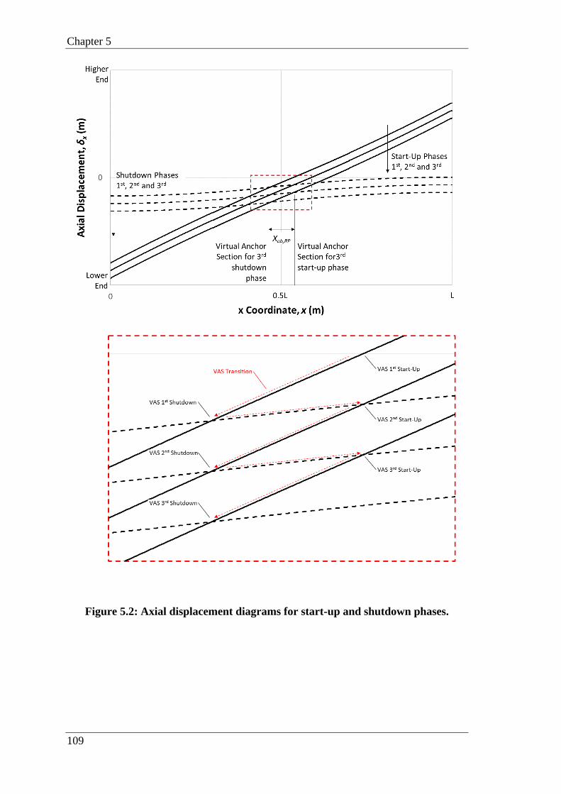
Chapter 5
109
Figure 5.2: Axial displacement diagrams for start-up and shutdown phases.
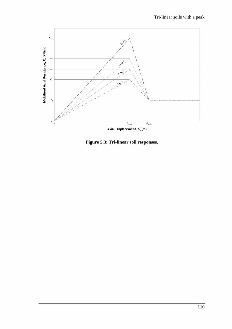
Tri-linear soils with a peak
110
Figure 5.3: Tri-linear soil responses.
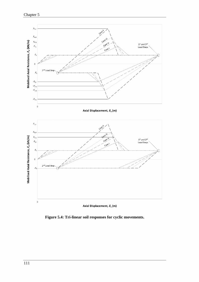
Chapter 5
111
Figure 5.4: Tri-linear soil responses for cyclic movements.

Tri-linear soils with a peak
112
Figure 5.5: Effective axial force for tri-linear strategy case ii – EqualPeaks (Zoom).

Chapter 5
113
Figure 5.6: Axial displacement for tri-linear strategy case ii – EqualPeaks (Zoom).
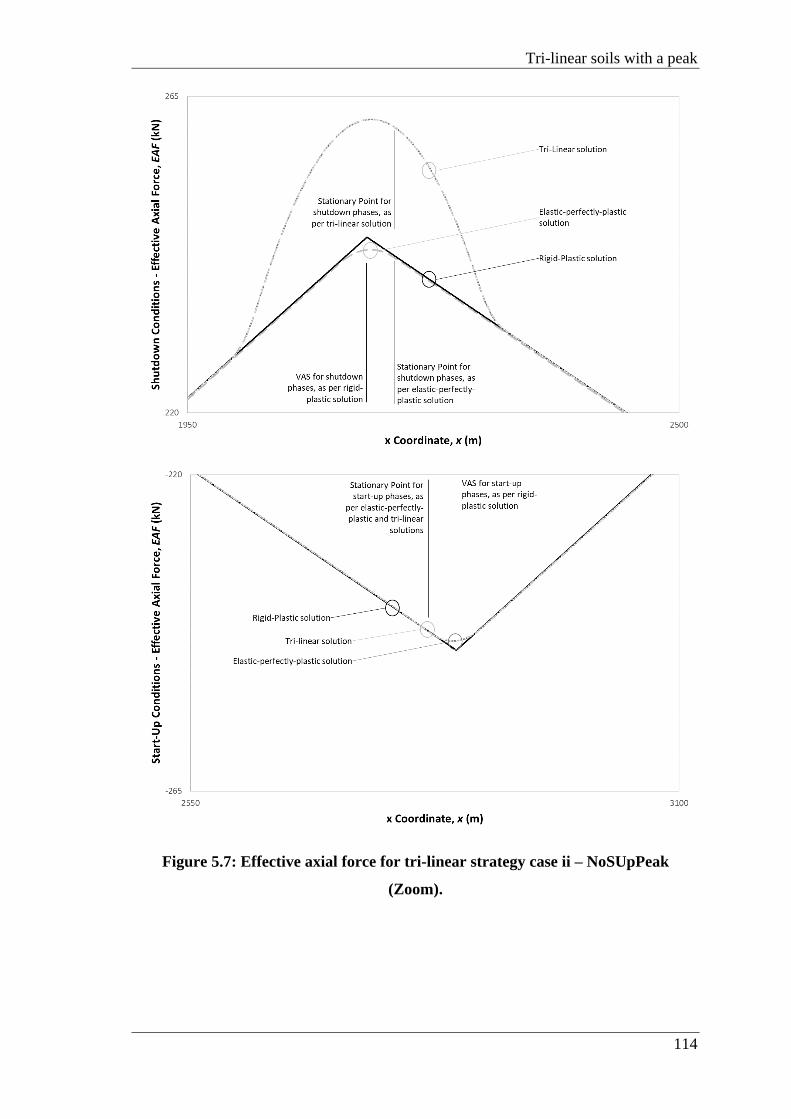
Tri-linear soils with a peak
114
Figure 5.7: Effective axial force for tri-linear strategy case ii – NoSUpPeak
(Zoom).

Chapter 5
115
Figure 5.8: Axial displacement for tri-linear strategy case ii– NoSUpPeak (Zoom).
Figure 5.9: Tri-linear correction results.

Tri-linear soils with a peak
116
Figure 5.10: Distance between stationary points results.
Figure 5.11: Walking rate results.

Chapter 6
117
CHAPTER 6. SOLVING DOWNSLOPE PIPELINE
WALKING ON NON-LINEAR SOIL WITH BRITTLE PEAK
STRENGTH AND STRAIN SOFTENING
Chapter context: This chapter presents the published paper which was prepared to show
that adjustments (similar to previous chapters) are required for the analytical assessment
of downslope pipeline walking phenomenon when non-linear with a peak pipe-soil
interactions are considered. It demonstrates that different non-linearities will alternatively
impact the assessments and how these impacts can be estimated.
This chapter contains material that has been prepared for publication as:
Castelo, A., White, D. and Tian, Y., 2017. Solving downslope pipeline walking on non-
linear soil with brittle peak strength and strain softening, OMAE2017-61168,
Proceedings of the International Conference on Ocean, Offshore and Arctic Engineering,
Trondheim, Norway
Non-linear soils with a peak
118
6.1 ABSTRACT
In 2000 the first case of pipeline walking (PW) was properly documented when this
phenomenon seriously impacted a North Sea high pressure and high temperature
(HP/HT) pipeline (Tornes et al., 2000).
On the other hand, to study other aspects related not only to PW, the industry joined
forces in the SAFEBUCK Joint Industry Project (JIP) with academic partners. As a result,
other drivers, which lead a pipeline to walk, have been identified (Bruton et al., 2010).
Nowadays, during the design stage of pipelines, estimates are calculated for pipeline
walking. These estimates often use a Rigid-Plastic (RP) soil idealization and the Coulomb
friction principle (Carr et al., 2006).
Unfortunately, this model does not reflect the real pipe-soil interaction behavior, and in
practice, time consuming finite element computations are often performed using an
Elastic-Perfectly-Plastic (EP) soil model. In reality, some observed axial pipe-soil
responses are extremely non-linear and present a brittle peak strength before a strain
softening response (White et al., 2011).
This inaccuracy of the soil representation normally overestimates the walking rate, WR,
(a rigid plastic soil model leads to greater walking). A magnified WR invariably leads to
false interpretations besides being unrealistic. Finally, a distorted WR might also demand
mitigating measures that could be avoided if the soil had been adequately treated.
Unnecessary mitigation has a very strong and negative effect on the project as whole. It
will require more financial and time investments for the entire development of the project
– from design to construction activities. Therefore, having more realistic and pertinent
estimates becomes valuable not only because of budgetary issues but also because of time
frame limits.
The present paper will show the results of a set of Finite Element Analyses (FEA)
performed for a case-study pipeline. The analyses – carried out on ABAQUS software –
used a specific subroutine code prepared to appropriately mimic Non- Linear Brittle Peak
with Strain Softening (NLBPSS) axial pipe-soil interaction behavior.
The specific subroutine code was represented in the Finite Element Models (FEMs) by a
series of User Elements (UELs) attached to the pipe elements.
The NLBPSS case is a late and exclusive contribution from the present work to the family

Chapter 6
119
of available pipeline walking solutions for different forms of axial pipe-soil interaction
model.
The parametric case-study results are benchmarked against theoretical calculations of
pipeline walking showing that the case study results deliver a reasonable accuracy level
and are reliable. The results are then distilled into a simplified method in which the WR
for NLBPSS soil can be estimated by adjusting a solution derived for RP and EP soil.
The key outcome is a genuine method to correct the WR resultant from a RP soil approach
to allow for peak and softening behaviour. It provides a design tool that extends beyond
the previously-available solutions and allows more rapid and efficient predictions of
pipeline walking to be made.
This contribution clarifies, for the downslope walking case, what is the most appropriate
basis to incorporate or idealize the soil characteristics within the axial Pipe-Soil
Interaction (PSI) response when performing PW assessments.
6.2 INTRODUCTION
6.2.1 Pipeline walking mechanisms
Pipeline walking is a long term cyclic movement of the pipeline in one direction, and can
be accompanied by an asymmetric build-up of effective force within the pipe due to a
restraint or a slope. The Pipeline Walking (PW) phenomenon was described in details by
Carr et al. (2006) and Bruton et al. (2010), who set out four driving mechanisms.
The mechanisms are:
• Seabed slope along the pipeline length;
• Tension at the end of the flowline (associated with a steel catenary riser - SCR);
• Thermal transients along the pipeline – leading to different temperature profiles
during Start-Up (SUp) and Shutdown (SDown);
• Multiphase fluid behavior during restart operations (e.g. gas-liquid separation on
SDown).
The most important aspect which relates these mechanisms to the phenomenon itself is
the fact that each of the mechanisms is able to create an asymmetry in the profile of axial
force along the pipeline. This loading asymmetry generally causes the appearance of the
pipeline walking, by causing unequal pipeline displacements during SUp and SDown
stages.

Non-linear soils with a peak
120
The present work is focused on the first mechanism listed above – the effect of seabed
slope – since this is the simplest case. However, the conclusions are applicable to all
mechanisms of pipeline walking.
6.2.2 Walking phenomenon on a rigid-plastic basis
When a pipeline is subjected to temperature and pressure increments it tends to expand
axially. This expansion will be resisted by the PSI forces – referred to simply as axial
friction – and effective compression will be induced into the pipeline.
On the other hand, when the same pipeline is exposed to temperature and pressure
decrements, it tends to contract and return to its original configuration. This time, the soil
reacts with a friction resisting force in the opposite direction in relation to the previous
behavior, introducing tension into the pipeline.
In the course of the SUp phase, considering a pipeline laid on the seabed and no
equipment attached to the pipeline (meaning that the ends are free and the soil resistance
is uniform), the effective axial compression develops from zero at pipeline ends to a
maximum value, approximately at its midlength point.
During the SDown phase, the pipeline temperature and internal pressure are set back to
their original (unloaded) values. In the same way, this tension will build up from zero at
the ends up to a maximum value approximately at the pipeline mid-length point.
For some pipelines, free of lateral buckling, the effective axial compression build up
occurs along sufficient length to induce compressive mechanical strain, which entirely
compensates the thermo-mechanical expansion. These are called “long” pipelines, while
those with insufficient effective axial compression are not able to fully compensate this
expansion, and are called “short” pipelines.
A non-anchored “short” pipeline, after contracting (SDown), may not go back to the same
position as previously on expansion (SUp). In this case, the cyclic expansion and
contraction behavior may result in geometric asymmetries between the expansion and
contraction cycles, if any of the four mechanisms listed above are present. These
asymmetries accumulate and cause large net axial global displacements over many
cycles.
Considering the case of a sloping seabed, it will cause a component of the pipe weight to
act parallel with the seabed in a downslope direction, while the axial friction will act in
interchanging directions opposing the current pipe movement direction. The effect of the

Chapter 6
121
interchanging component direction will also impact the effective compression and
tension along the pipeline length during its operational lifetime.
Figure 6.1 presents an example of effective axial force (EAF) diagram for the SUp
condition, showing the profile of EAF accounting for both slope and soil friction. As
sketched, the downslope weight component is added to or subtracted from the nominal
soil resistance. Therefore, the force diagram is not symmetrical and the maximum point,
corresponding to the Stationary Point (SP) on the pipe, is not at its mid-point.
Figure 6.2 shows the asymmetry between the effective compression and tension profiles,
due to the weight component always acting downwards. It can be noted that this
asymmetry causes an offset between the SPs for the SUp and SDown conditions.
Figure 6.3a shows the axial displacement (δx) for the first SUp phase, highlighting the
stationary point after 0.5L. The aforementioned temperature increase generates this
behavior. Figure 6.3b presents how the pipeline contracts without moving to its original
position, when the temperature decreases – for the first SDown step. The SPSDown lies
at the pipe section where the diagrams cross, as indicated, before 0.5L.
During the next or second loading cycle (Figure 6.4a), the intersection point is back after
0.5L; and when unloaded, before 0.5L again. Figure 4a also indicates the net axial shift,
which is induced by the difference between the SPs. Loaded and unloaded graphs for the
second cycle are similar to those for first cycle, but offset by this net axial shift, which
might typically be of some centimeters. Figure 6.4b shows how this shift accumulates
through 3 cycles, possibly resulting in several meters of longitudinal displacement over
the lifetime of the pipeline.
These results illustrate the axial ratcheting induced by an overall slope in the bathymetry,
which is only one of the pipeline walking drivers and is the case considered in the present
work.
6.2.3 Walking consequences
The pipeline walking phenomenon is not a limit state itself, but it may lead to several
other design challenges (Bruton et al., 2010), such as:
• Overstressing connections;
• Loss of tension in a SCR;
• Increase the loading in a lateral buckling;
• Route instability (curve pull out).
Non-linear soils with a peak
122
Any of the listed consequences might lead the pipeline system to fail, locally or globally;
and, they might appear separately or associated to other mentioned consequences.
Hence, the phenomenon and its consequences must be prevented in order to keep the
safety of the system and its entire environment.
On the other hand, simplifying the PSI behavior for PW assessments might not be
beneficial for the project. Inaccurately representing the PSI performance might lead to
overestimates of WR.
Besides being unrealistic, the referred overestimates regularly bring misunderstandings
to the design activities. A magnified WR might require mitigation to PW, which could be
avoided if the soil was properly described.
Mitigation activities have a very strong impact in any project. From designing to
installing the mitigation devices, more time and capital will be needed.
Therefore, it is essential to properly represent the PSI, so that the project can be
adequately developed avoiding any unnecessary expenditure.
6.2.4 Axial pipe-soil non-linearity
Model testing in the laboratory and at the seabed has shown that the axial pipe-soil
response is extremely non-linear. The magnitude of the axial pipe-soil friction coefficient
depends on the soil strength, pipe roughness and the drainage condition – White et al.
(2011) and White et al. (2012) – but these effects are beyond the scope of the present
study. Instead, the focus of this study is on the shape of the axial load displacement
response during both loading and unloading.
In the present paper, the soil considered is a soft natural clay as per the one presented by
White et al. (2011), although some parameters have been adjusted for this work. The aim
of this work is to show how more accurate PSI responses can be incorporated in a PW
assessment, because this offers a clear advance to the methodology of design compared
to the one currently applied by industry, which might be regarded as a too simply design
approach, that carries unwanted consequences in relation to more onerous walking
mitigation requirements.
The axial resistance measured during a typical cycle of movement from a field test using
an in situ testing tool is shown in Figure 6.5a, which is based on previously published
data (White et al., 2011). The extremely nonlinear axial response shows a smooth
transition between an initial high tangent stiffness which reduces until it reaches a zero

Chapter 6
123
tangent stiffness at a limiting axial friction. This limiting axial friction represents a peak
resistance which is followed by a negative tangent stiffness taking the resistance to a
residual/ plastic plateau.
In other words, this soil presents a brittle peak strength with a strain softening resistance,
which is the approximated non-linear behavior used in the present work.
For the present study, the non-linearity of the axial response has been captured using a
non-linear spring-slider of the form illustrated in Figure 6.5b.
It is important to stress, at this point, that Figure 6.5b also serves the purpose of
contrasting the soil model used by the present work and how the current methodology
considers the soil spring.
The non-linear approach is used by this paper, while the current industry methodology
usually uses the Rigid-Plastic approach (Figure 6.5b).
6.3 PROBLEM DEFINITION
6.3.1 General Properties of Study-Case
As mentioned previously, this paper considers a pipeline resting on a sloped seabed. The
case study considers a straight steel pipeline, laid on a uniformly sloped seabed.
The general properties are shown in Table 6.1.
Table 6.1: Pipeline properties.
Property Value
Steel Outside Diameter, OD 0.3239m
Steel Wall Thickness, t 0.0206m
Water Depth, D 1200m
Length, L 5000m
Seabed Slope, β 2.0°
Axial Friction Coefficient, µ 0.25
Temperature Variation, ΔT 100°C
Pipe Submerged Weight, W 0.4kN/m
Steel Young's Modulus, E 2.07x10¹¹Pa

Non-linear soils with a peak
124
Steel Poisson Coefficient, ν 0.3
Steel Thermal Expansion Coefficient, α 1.165x10⁻⁵°C-1
The pipe operational submerged weight, W, has been calculated considering the overall
volume of steel and content in one meter of pipe. Then, the one meter volume has been
used, along with the specific density of each material, to calculate the final buoyancy per
meter of pipe (plus contents), as per Archimedes’ Principle.
6.3.2 Variations in axial pipe-soil response
Two different pipe-soil property sets have been considered for the numerical analysis
(Case A and Case B). Axial pipe-soil resistance has been modelled based on the example
illustrated in Figure 6.6, adopting the parameters given in Table 6.2.
Table 6.2: Axial pipe-soil interaction model parameters.
Property Case A Case B
Limiting Displacement 1, δ1 0.049m 0.012m
Limiting Displacement 2, δ2 0.081m 0.081m
Limiting Displacement 3, δ3 0.097m 0.097m
Limiting Displacement 4, δ4 0.115m 0.115m
Limiting Force 1, F1 0.150kN 0.050kN
Limiting Force 2, F2 0.200kN 0.200kN
Limiting Force 3, F3 0.150kN 0.150kN
Limiting Force 4, F4 0.100kN 0.100kN
As can be seen from the parameters presented in Table 6.2, the main difference among
Cases A and B was the limit defining the interaction between linear-elastic and parabola
1 behaviors.
For Case A, the couple (δ1,F1) lies above the plastic residual plateau (F4), while for case
B it lies below the same plateau – Figure 6.6; and, the present work examines the
divergence originated from this aspect.
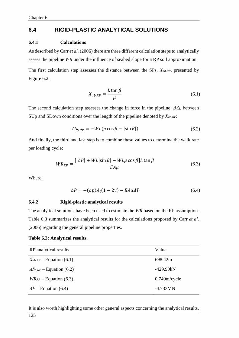
Chapter 6
125
6.4 RIGID-PLASTIC ANALYTICAL SOLUTIONS
6.4.1 Calculations
As described by Carr et al. (2006) there are three different calculation steps to analytically
assess the pipeline WR under the influence of seabed slope for a RP soil approximation.
The first calculation step assesses the distance between the SPs, Xab,RP, presented by
Figure 6.2:
𝑋𝑎𝑏,𝑅𝑃 =𝐿 tan𝛽
𝜇 (6.1)
The second calculation step assesses the change in force in the pipeline, ΔSS, between
SUp and SDown conditions over the length of the pipeline denoted by Xab,RP:
𝛥𝑆𝑆,𝑅𝑃 = −𝑊𝐿(𝜇 cos 𝛽 − |sin 𝛽|) (6.2)
And finally, the third and last step is to combine these values to determine the walk rate
per loading cycle:
𝑊𝑅𝑅𝑃 =[|𝛥𝑃| +𝑊𝐿|sin 𝛽| −𝑊𝐿𝜇 cos 𝛽]𝐿 tan 𝛽
𝐸𝐴𝜇 (6.3)
Where:
𝛥𝑃 = −(𝛥𝑝)𝐴𝑖(1 − 2𝜈) − 𝐸𝐴𝛼𝛥𝑇 (6.4)
6.4.2 Rigid-plastic analytical results
The analytical solutions have been used to estimate the WR based on the RP assumption.
Table 6.3 summarizes the analytical results for the calculations proposed by Carr et al.
(2006) regarding the general pipeline properties.
Table 6.3: Analytical results.
RP analytical results Value
Xab,RP – Equation (6.1) 698.42m
ΔSS,RP – Equation (6.2) -429.90kN
WRRP – Equation (6.3) 0.740m/cycle
ΔP – Equation (6.4) -4.733MN
It is also worth highlighting some other general aspects concerning the analytical results.

Non-linear soils with a peak
126
Table 6.4 shows the values of these important characteristics.
Table 6.4: Key aspects from rigid-plastic solution.
General Aspects Value
SUp Max Compression Force -245kN
SUp Max Compression Force Position 2849m
SDown Max Tension Force 245kN
SDown Max Tension Force Position 2151m
SUp Stationary Point 2849m
SDown Stationary Point 2151m
Figure 6.7 shows the EAF plot in regards of the RP basis and also provides some details
about the key aspects of RP solution from Table 6.4.
At this stage, it is important to emphasize that for RP soils, SPs are the same as the
maximum EAF positions. This is not true for other soil idealizations as described by
Castelo et al. (2019).
6.5 NLBPSS FEM SOLUTION
The FEM used for this paper was a geometrically simplified model, based on a one-
dimensional pipeline laid on a uniformly sloped seabed and its general properties were
presented in Table 6.1.
6.5.1 FEM architecture
The pipeline was represented by 5001 nodes connected between them by 5000 B33 (three
dimensional three node element) pipe elements (see Dassaul, (2014) for technical details).
The soil was modeled as non-linear spring elements connected to each pipeline element
(at the pipeline nodes). Such elements were designed as UELs via a subroutine
specifically coded in FORTRAN language for this paper.
Loads
The loads acting on the pipeline are related to self-weight and temperature only.
The effect of the uniform slope is accounted for as a longitudinal load equivalent to the
component of the pipeline weight, as given by:

Chapter 6
127
𝑊𝑐𝑜𝑚𝑝 = 𝑊 sin 𝛽 (6.5)
The operational cycling was done taking in account the steady operational profile (SUp)
and the rest condition (SDown). No intermediate step of loading was manually included.
The SUp and SDown temperatures were accounted as per Table 6.1.
Pipe-soil interaction representation
As aforementioned (Sections 6.2.4 and 6.2.4), the way used to represent the PSI was
through UELs coded in FORTRAN. The basic philosophy for the UEL was an initially
linear relation between displacement and reaction force with a constant stiffness until a
limit displacement/ force couple was achieved (δ1,F1). Then a variable and decreasing
stiffness would be provided until a second limit couple was reached (δ2,F2), where the
tangential stiffness reaches ZERO. Then, the stiffness would face a negative stretch going
through the couple (δ3,F3), until reaching a zero tangent stiffness again at (δ4,F4), where
the plastic plateau is imposed to any further displacement (at the current step).
However, the spring load history will impact the load succession as can be seen in Figure
6.8, where the different possible behaviors are schematically represented. The choice of
tangent stiffness for the next step is determined depending on the axial displacement in
the current step, UA_m, relative to the axial displacement in the previous step, UA_Ref.
For a positive displacement (UA_m - UA_Ref > 0), behaviors 1 and 2 control the spring
response depending on the initial spring force of reference, FS_Ref. If FS_Ref is bigger
than the elastic limit, Felastic, it falls into behavior 2 regime; otherwise, it remains behavior
1 regime.
For negative displacements, behaviors -1 and -2 control the spring response mirroring the
relationship between behaviors 1 and 2.
In order to provide a better understanding about the general FORTRAN subroutine logic,
a simplified flowchart is included in Figure 6.9.
The governing equation for a parabola, which is differentiated to give the tangent stiffness
at different steps, is:
𝑓(𝑥) = 𝐴𝑥2 + 𝐵𝑥 + 𝐶 (6.6)
In case a higher order of non-linearity shall be modelled, perhaps to give a better fit to
field test results, a higher order polynomial may be used or an alternative formulation, so
that it represents a better fit for the soil behavior. In other words, Figure 6.6 will show

Non-linear soils with a peak
128
more boundaries, i.e. more pairs (δ,F).
It is important to stress that FS_Ref is a just a memory entry automatically kept from the
previous iteration to the next. So, it does not really matter the displacement direction for
FS_Ref, it is just the previous resultant force, FS_m.
An extensive and exhaustive test routine was performed to verify the User Element
reliability when put to use for the walking analyses. Firstly, a single node ‘floating’ in
space would be connected to the UEL, and this point would be displaced in order to
activate the spring subroutine generating a resultant force; then, the result would be cross
checked with the preconceived NLBPSS spring – based on White et al. (2011).
Afterwards, a piece of pipe would be modelled and connected to some UELs. The same
overall displacement steps would be followed and the resultant force compared. Given
that all results, generated by displacement controlled loads, agreed with the designed
NLBPSS soil curve, it was put to practice with force loads generated by thermal
increments.
At this stage, all nodes from the aforementioned “single pipe element” tests were closely
observed to guarantee that their resultant reaction force would still agree with the desired
NLBPSS curve. Finally, after reassuring that all results respected the original non-linear
soil spring, the subroutine was awarded a “reliable” status and full length pipeline
analyses were carried out.
The results using this soil approximation show how the non-linearity of a soil model with
brittle peak strength and strain softening affects the WR.
6.5.2 FEM results
In this section, we discuss the different results of the FEMs in terms of EAF and δx in
order to summarize and to highlight important aspects concerning the results that have an
influence on the PW.
FEM results
Figure 6.10 shows the results, in terms of EAF, along the entire pipeline length for five
load cycles – both cases are presented: Case A – Figure 6.10a and Case B – Figure 6.10b.
Figure 6.11 shows the same results, but this time zooming into the vicinity of the Max
and Min Forces region – both cases are presented: Case A and Case B are shown in Figure
6.11a and Figure 6.11b, respectively.
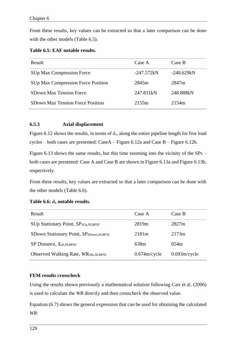
Chapter 6
129
From these results, key values can be extracted so that a later comparison can be done
with the other models (Table 6.5).
Table 6.5: EAF notable results.
Result Case A Case B
SUp Max Compression Force -247.572kN -248.629kN
SUp Max Compression Force Position 2845m 2847m
SDown Max Tension Force 247.831kN 248.888kN
SDown Max Tension Force Position 2155m 2154m
6.5.3 Axial displacement
Figure 6.12 shows the results, in terms of δx, along the entire pipeline length for five load
cycles – both cases are presented: CaseA – Figure 6.12a and Case B – Figure 6.12b.
Figure 6.13 shows the same results, but this time zooming into the vicinity of the SPs –
both cases are presented: Case A and Case B are shown in Figure 6.13a and Figure 6.13b,
respectively.
From these results, key values are extracted so that a later comparison can be done with
the other models (Table 6.6).
Table 6.6: δx notable results.
Result Case A Case B
SUp Stationary Point, SPSUp,NLBPSS 2819m 2827m
SDown Stationary Point, SPSDown,NLBPSS 2181m 2173m
SP Distance, Xab,NLBPSS 638m 654m
Observed Walking Rate, WRObs,NLBPSS 0.674m/cycle 0.693m/cycle
FEM results crosscheck
Using the results shown previously a mathematical solution following Carr et al. (2006)
is used to calculate the WR directly and then crosscheck the observed value.
Equation (6.7) shows the general expression that can be used for obtaining the calculated
WR:
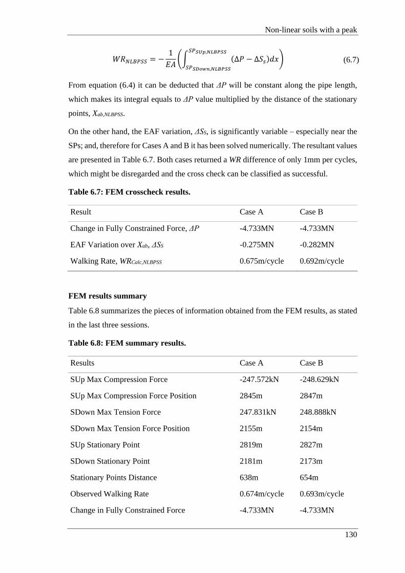
Non-linear soils with a peak
130
𝑊𝑅𝑁𝐿𝐵𝑃𝑆𝑆 = −1
𝐸𝐴(∫ (∆𝑃 − ∆𝑆𝑠)𝑑𝑥
𝑆𝑃𝑆𝑈𝑝,𝑁𝐿𝐵𝑃𝑆𝑆
𝑆𝑃𝑆𝐷𝑜𝑤𝑛,𝑁𝐿𝐵𝑃𝑆𝑆
) (6.7)
From equation (6.4) it can be deducted that ΔP will be constant along the pipe length,
which makes its integral equals to ΔP value multiplied by the distance of the stationary
points, Xab,NLBPSS.
On the other hand, the EAF variation, ΔSS, is significantly variable – especially near the
SPs; and, therefore for Cases A and B it has been solved numerically. The resultant values
are presented in Table 6.7. Both cases returned a WR difference of only 1mm per cycles,
which might be disregarded and the cross check can be classified as successful.
Table 6.7: FEM crosscheck results.
Result Case A Case B
Change in Fully Constrained Force, ΔP -4.733MN -4.733MN
EAF Variation over Xab, ΔSS -0.275MN -0.282MN
Walking Rate, WRCalc,NLBPSS 0.675m/cycle 0.692m/cycle
FEM results summary
Table 6.8 summarizes the pieces of information obtained from the FEM results, as stated
in the last three sessions.
Table 6.8: FEM summary results.
Results Case A Case B
SUp Max Compression Force -247.572kN -248.629kN
SUp Max Compression Force Position 2845m 2847m
SDown Max Tension Force 247.831kN 248.888kN
SDown Max Tension Force Position 2155m 2154m
SUp Stationary Point 2819m 2827m
SDown Stationary Point 2181m 2173m
Stationary Points Distance 638m 654m
Observed Walking Rate 0.674m/cycle 0.693m/cycle
Change in Fully Constrained Force -4.733MN -4.733MN

Chapter 6
131
EAF Variation Over Xab -0.275MN -0.282MN
Calculated Walking Rate 0.675m/cycle 0.692m/cycle
Taking into account that a 1m mesh was included in the calculated results (due to the
models architecture), the error between the FEA WR and the directly calculated value is
negligible. For consistency, the FEM results are used in the further analysis.
6.6 RESULTS COMPARISON
6.6.1 Effective axial force
Table 6.9 compares can be formed to help comparing the EAF results.
Table 6.9: EAF comparison.
Results RP Case A Case B
SUp Max Compression Force -245kN -247.572kN -248.629kN
SUp Max Compression Force Position 2849m 2845m 2847m
SDown Max Tension Force 245kN 247.831kN 248.888kN
SDown Max Tension Force Position 2151m 2155m 2154m
Approximately, the comparison between FEM and Analytical results leads to the
conclusion that the maximum values of EAF and their positions are all very similar. These
changes alone do not explain the observed change in WR.
6.6.2 Stationary points
Looking only at the SPs results, Table 6.10 is prepared, so that it becomes easier to
compare SPs results.
Table 6.10: SPs comparison.
Results RP Case A Case B
SPSUp 2849m 2819m 2827m
SPSDown 2151m 2181m 2173m
Xab 698m 638m 654m

Non-linear soils with a peak
132
Observing the SP results, the change was more dramatic than the ones observed in the
previous item (6.6.1). Case A showed a 60m change in the distance between the SPs;
while, Case B reduced Xab about 44m.
Although the soil models – for Cases A and B – present a prominent peaky behavior, the
variations observed for the SPs, as stressed in the previous paragraph, agrees with the
expected behavior, as established – for non-peak cases – in other work (Castelo et al.,
2019, in press).
Previous similar studies show that the peaky behaviors have no major influence on the
walking phenomenon relative to the same soil response but with no peak, so the peak
impact may be disregarded for this scope of the present work (Castelo et al. 2019).
Therefore, the distance between the stationary points observed for Case A returned a
value that can be approximately considered equal to – as per (Castelo et al., in press a):
𝑋𝑎𝑏,3𝐿 = 𝑋𝑎𝑏,𝑅𝑃 (1 −𝐹𝑅𝐹𝑃
𝛿𝑚𝑜𝑏𝑃𝛿𝑛𝑢𝑙𝑙
) (6.8)
where δmobP is the peak mobilisation distance, FR and FP are the residual force level and
the peak force level, respectively; and δnull is an idealization for non-linear soil
approaches to represent a mobilisation distance at which walking ceases (Castelo et al.,
2019). In the present work, this has a value of δnull = 0.370m for both cases considered.
For Case B, equation (6.8) does not derive into a direct relation between the observed
FEM results and the equation products. Therefore, some algebra can be used on equation
(6.8) to generate a more general equation – alternatively to (Castelo, et al., in press b):
𝑋𝑎𝑏,𝑁𝐿𝐵𝑃𝑆𝑆 = 𝑋𝑎𝑏,𝑅𝑃 (1 −𝛿𝑚𝑜𝑏𝐸𝑄𝛿𝑛𝑢𝑙𝑙
) (6.9)
where δmobEQ is an equivalent mobilisation distance to be later explored (Section 6.7).
6.6.3 Axial displacements & walking rates
The walking rate results are now presented. Table 6.11 shows only the WR results (for
the FEM Cases A and B, the observed values were accounted for, as already clarified).
Table 6.11: Walking rates for different soil approaches.
Result RP Case A Case B
WR 0.740m/cycle 0.674 m/cycle 0.693 m/cycle

Chapter 6
133
From Table 6.11, it can be clearly seen that the WR results also varied between the RP
and NLBPSS cases, by 10%.
Again, Case A results agree with the explanation given by Castelo et al. (in press a) that
for peaky soils the WR can be calculated as:
𝑊𝑅3𝐿 = 𝑊𝑅𝑅𝑃 ∗ (1 −𝐹𝑅𝐹𝑃
𝛿𝑚𝑜𝑏𝑃𝛿𝑛𝑢𝑙𝑙
) (6.10)
However, Case B does not completely match equation (6.10) definition, which requires
a further generalization as – in accordance with Castelo et al. (in press b):
𝑊𝑅𝑁𝐿𝐵𝑃𝑆𝑆 = 𝑊𝑅𝑅𝑃 ∗ (1 −𝛿𝑚𝑜𝑏𝐸𝑄𝛿𝑛𝑢𝑙𝑙
) (6.11)
6.7 EQUIVALENT MOBILISATION DISTANCE
Other research (Castelo et al., 2019, in press b, in press a) indicates that the equivalent
mobilisation distance, δmobEQ, can be obtained from dividing the unload-reload area (as
per Figure 6.14) by the residual force variation (ΔFR) – as per equation (6.12):
𝛿𝑚𝑜𝑏𝐸𝑄 = (𝐴𝑈𝑛𝑙𝑜𝑎𝑑−𝑅𝑒𝑙𝑜𝑎𝑑
𝛥𝐹𝑅) (6.12)
Figure 6.14a and Figure 6.14b show the properties involved in obtaining δmobEQ for Cases
A and B, respectively.
Considering the values and the given method in Figure 6.14, Case A provides a δmobEQ of
0.032390m, while Case B has a δmobEQ equals to 0.024872m.
6.7.1 Back evaluation
Naturally, the next step for this paper is to check the hypothesis given by the equivalent
mobilisation distance approach (equation (6.8)) so that it can be proved correct.
Then, equations (6.9) and (6.11) will be evaluated and contrasted against the FEM results
formerly presented (Sections 6.5 and 6.6).
Table 6.12: Equations (6.9) and (6.11) results.
Results Case A Case B
Xab – Equation (6.9) 637m 652m

Non-linear soils with a peak
134
WR – Equation (6.11) 0.675m/cycle 0.690m/cycle
Analyzing the distance between the stationary points, Xab, equation (6.9) provides a good
estimative within a 0.31% margin of error. 637m and 652m are obtained from equation
(6.9), for Case A and Case B, respectively; while the FEM results indicated 638m and
654m for cases A and B.
Now, checking the results of walking rate, WR, equation (6.11) also derives into results
with a good agreement with the FEM results with an acceptable and marginal deviation
(0.43%). Equation (6.11) delivers a WR of 0.675 and 0.690m/cycle for cases A and B. At
the same time, the FEM approach 0.674 and 0.693 m/cycle for A and B.
Therefore, the back evaluation concerning equations (6.9) and (6.11) can be classified as
successful. A wider set of results exploring this approach, and similar efficient walking
rate analysis methods are given in Castelo et al. (2019, in press b, in press a). These offer
a tool to assist in future walking assessments.
6.8 CONCLUSIONS & FINAL REMARKS
The industry has seen the influence from some phenomena, such as pipeline walking,
increase; as hydrocarbons reservoirs have become more difficult to access over the last
decades, leading to higher wellstream temperatures in deeper and colder waters.
Some research has been done on PW; but, it was still not fully understood how this
problem should be really treated since distortions have been noticed between several
design assessments and operational observations.
The models presented in this paper provide new insights into axial PSI and its impact on
PW evaluations.
Thus, the parametric study presented by the present work, led to a better understanding
on how PW can be assessed when a highly non-linear peaky axial PSI is observed on soil
tests. Then, in order to correct the analytical assessments based on RP basis, originally
proposed by Carr et al. (2006), a new calculation approach is suggested.
It is shown that the non-linear soil model can be simplified to determine an equivalent
mobilisation distance – for an equivalent linear elastic perfectly plastic model – and this
value can be used to give an adjustment to the rigid plastic walking rate solution (from
Carr et al. (2006)) to give the walking rate on non-linear peaky soil.

Chapter 6
135
FIGURES
Figure 6.1: EAF diagram and sketch of acting loads.
Figure 6.2: EAF diagrams for start-up and shutdown.

Non-linear soils with a peak
136
Figure 6.3: Axial displacement – 1st cycle.

Chapter 6
137
Figure 6.4: Axial displacement – further cycles.

Non-linear soils with a peak
138
Figure 6.5: Axial PSI non-linear approach.

Chapter 6
139
Figure 6.6: Axial PSI boundaries.
Figure 6.7: Analytical EAF plot.

Non-linear soils with a peak
140
Figure 6.8: Schematic behaviours plot.

Chapter 6
141
Figure 6.9: Subroutine flowchart.
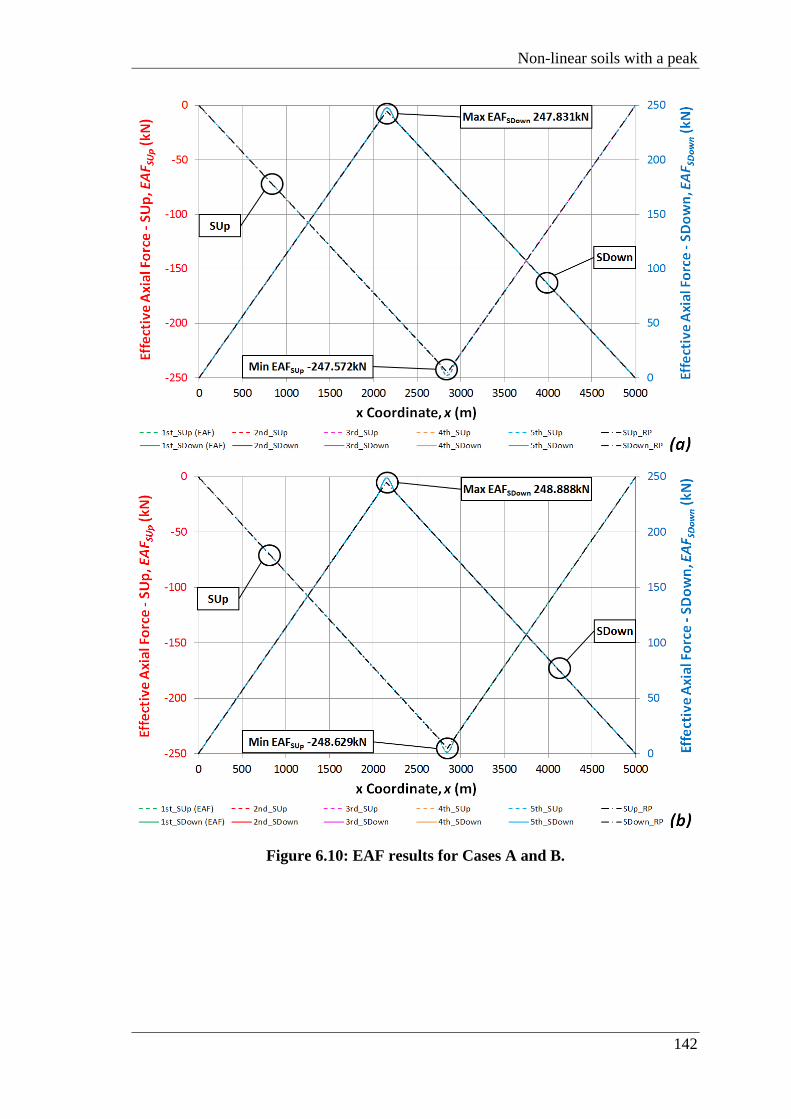
Non-linear soils with a peak
142
Figure 6.10: EAF results for Cases A and B.

Chapter 6
143
Figure 6.11: EAF zoom for Cases A and B.
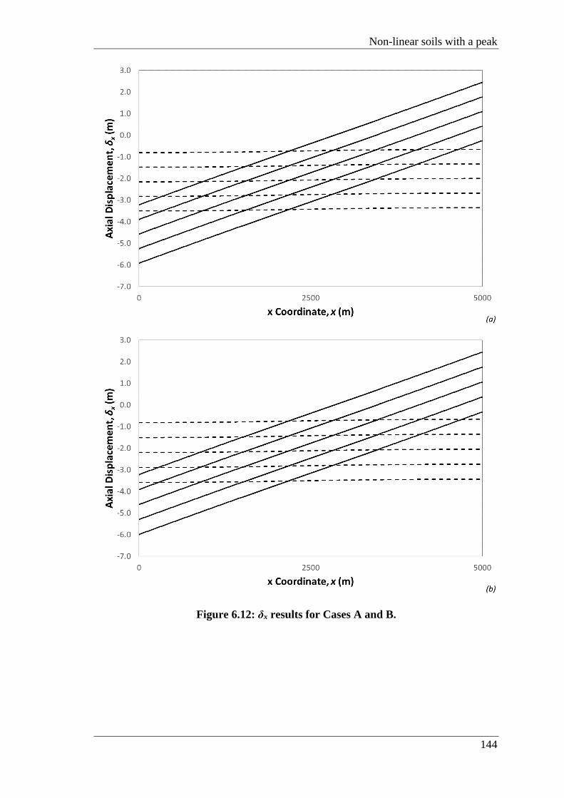
Non-linear soils with a peak
144
Figure 6.12: δx results for Cases A and B.
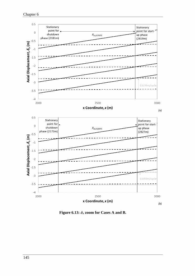
Chapter 6
145
Figure 6.13: δx zoom for Cases A and B.

Non-linear soils with a peak
146
Figure 6.14: Obtaining δmobEQ – for Cases A and B.
Chapter 7
147
CHAPTER 7. GRAVITY-DRIVEN PIPELINE WALKING
ON VARIABLE SLOPES
Chapter context: In this thesis’ chapter, variable slopes are covered. This chapter was
motivated by the lack in the literature of verification for applicability on variable slopes
topography. It brings the previous chapters closer to real-world conditions, where
pipeline routes vary in slope topography alongside with pipe-soil interaction behaviours.
This chapter contains material that has been prepared for publication as:
Castelo, A., White, D. and Tian, Y., in press. Gravity-driven pipeline walking on variable
slopes. International Journal of Offshore and Polar Engineering (submitted to journal)
Variable slopes
148
7.1 ABSTRACT
Gravity-driven pipeline walking is a phenomenon where a pipeline migrates globally
downslope at a certain rate per loading cycle. It can significantly impact the subsea
system integrity and influences the design. The current methodology simplifies the
geometry by assuming a uniform slope along the entire route. However, real pipelines
traverse routes that slope with varying angles. The literature lacks evidence to justify such
simplification. Motivated by this, this study establishes whether uniform slope solutions
can be applied. The applicability of emerging research is also confirmed, allowing a
realistic representation of pipe-soil interaction.
7.2 INTRODUCTION
As oil and gas activities increasingly moves to deep water reservoirs, pipelines become
more important. Under operational conditions, pipelines will expand and contract due to
temperature and pressure changes. These expansion and contraction cycles might be
asymmetric because of seabed slopes or other factors, as explained by Carr et al. (2006)
and Bruton et al. (2010). As a result of this asymmetry, pipelines’ stability may be
seriously compromised, and they may globally migrate in one direction, in a phenomenon
known as pipeline walking (Carr et al., 2003).
Pipeline walking increases cost and risk and may greatly impact subsea systems (Tornes
et al., 2000). Connections may be overstressed, loads may be increased, initiating lateral
buckling, and ultimately the pipeline will need to be anchored. Therefore, properly
identifying and quantifying pipeline walking is of paramount importance to decrease risk
of production loss and environmental damage besides also reducing project development
costs.
Currently, the industry common practice is to carry out a pipeline walking evaluation in
the design phase using a set of analytical formulations, which consider a simplified
geometry by assuming a uniform slope along the entire pipeline route, from one end to
the other (Bruton et al., 2010). These calculations consider various aspects, such as
operational factors (temperature, pressure, etc.), environmental factors (seabed overall
slope angle, soil friction, etc.) and physical pipeline properties (length, steel wall
thickness, etc.).
On the other hand, real pipelines traverse routes that often slope continuously down, but

Chapter 7
149
at a varying angle (Leckie et al., 2016). Hence, adequately understanding and estimating
gravity-driven downslope pipeline walking for pipelines laid on variable slope seabeds is
extremely important since this condition is commonly found in fully operational areas,
such as Northwest Australia and West Africa, as well as in frontier locations, which are
in early stages of exploration, such as the Brazilian Pre-Salt and the Arctic Region.
However, the analytical expressions (Bruton et al., 2010) are known to provide inaccurate
walking rates, thus necessitating further analyses to overcome the known limitations. To
solve some of these limitations, emerging academic research (Castelo et al., 2017)
demonstrated that, if the adequate soil behavior is considered in the initial analytical
formulae, accurate walking rates can be easily achieved by including a reduction factor
based on the soil characteristics.
Although the formulation developed by Castelo et al. (2017) represents an improvement
in the available knowledge, it was limited to a uniform slope assumption. Therefore,
motivated by this, the present paper investigates whether uniform slope solutions can be
successfully applied to variable slope condition, by averaging the slope to be uniform
throughout the entire route using an average seabed slope, βave.
Unfortunately, there is no detailed data of field measurements or laboratory tests in the
currently available literature on downslope pipeline walking; although it is known that
operators across the globe keep track of their pipelines’ movements. Therefore, this paper
presents a numerical study, to benchmark and validate the analytical findings, which
considers a total of 104 finite element models. 52 models have a dual slope topography
(26 convex and 26 concave shapes), while the remaining 52 have a triple slope
topography (26 flat-slope-flat and 26 slope-flat-slope shapes).
Across the currently available literature, various slopes have been noticed. Some authors
register very gentle slopes, such as 0.22° (Jayson et al., 2008); while other pipelines have
presented more extreme slope angles, such as 10° (Kumar and Mcshane, 2009). For the
groups of 26 models, 13 considered gentle slopes (1° to 5°), while the remaining 13
considered extreme angles (6° to 10°) as well.
7.3 BACKGROUND TO PIPELINE WALKING
7.3.1 Downslope walking mechanisms
The seabed slope generates an asymmetry between the start-up and shutdown phases in

Variable slopes
150
the effective axial force profile for a fully mobilized pipeline, as illustrated in Figure 7.1
where the rigid-plastic soil condition is considered (Bruton et al., 2010).
This asymmetry causes the Virtual Anchor Sections (VAS), which are the non-moving
sections of the pipeline during the different load steps, to be separated by a given distance,
Xab. For rigid-plastic (RP) soil conditions, the virtual anchor sections correspond to the
maximum absolute effective force along the pipeline length, as proved by Castelo et al.
(2019). Then, the distance Xab can be associated to the axial displacement, δx, from a
particular load cycle, as represented by Figure 7.2.
Because it tends to create unbalanced displacements during different loading phases, the
asymmetry in the effective axial force profile is presently understood to be the root cause
of pipeline walking.
Accounting for more realistic soil conditions, the distance Xab cannot be associated with
the maxima effective axial force sections. Therefore, Xab must be associated with the
stationary points, as thoroughly explained in Castelo et al. (2019).
7.3.2 Route topography
Although previous research on pipeline walking has explored different geotechnical
aspects, no investigation on variable slopes along the pipeline route was conducted.
Different soil idealizations (Bruton et al., 2010; Castelo et al., 2019), and realistic soils
(Castelo et al., 2017) have been scrutinized in regards of their impact on pipeline walking.
Hence, this paper focuses solely on the impact variable slopes may have on pipeline
walking.
To conduct this investigation, a numerical study has been conducted including a set of
104 models, which consider 4 different topographies for 2 different slopes’ range (gentle
and extreme angles).
7.4 PROBLEM DEFINITION
Downslope pipeline walking depends on three different kinds of properties:
environmental, operational and those of the pipeline. This paper’s numerical study uses
typical property ranges.
The environmental parameters include seabed slopes, β, mobilisation distance, δmob, and
axial residual friction coefficient, μ, as shown in Table 7.1.
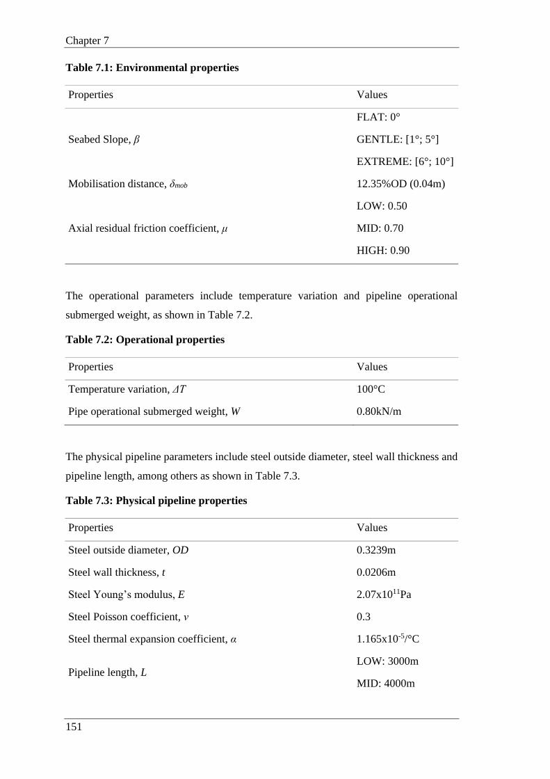
Chapter 7
151
Table 7.1: Environmental properties
Properties Values
Seabed Slope, β
FLAT: 0°
GENTLE: [1°; 5°]
EXTREME: [6°; 10°]
Mobilisation distance, δmob 12.35%OD (0.04m)
Axial residual friction coefficient, μ
LOW: 0.50
MID: 0.70
HIGH: 0.90
The operational parameters include temperature variation and pipeline operational
submerged weight, as shown in Table 7.2.
Table 7.2: Operational properties
Properties Values
Temperature variation, ΔT 100°C
Pipe operational submerged weight, W 0.80kN/m
The physical pipeline parameters include steel outside diameter, steel wall thickness and
pipeline length, among others as shown in Table 7.3.
Table 7.3: Physical pipeline properties
Properties Values
Steel outside diameter, OD 0.3239m
Steel wall thickness, t 0.0206m
Steel Young’s modulus, E 2.07x10¹¹Pa
Steel Poisson coefficient, ν 0.3
Steel thermal expansion coefficient, α 1.165x10⁻⁵/°C
Pipeline length, L LOW: 3000m
MID: 4000m
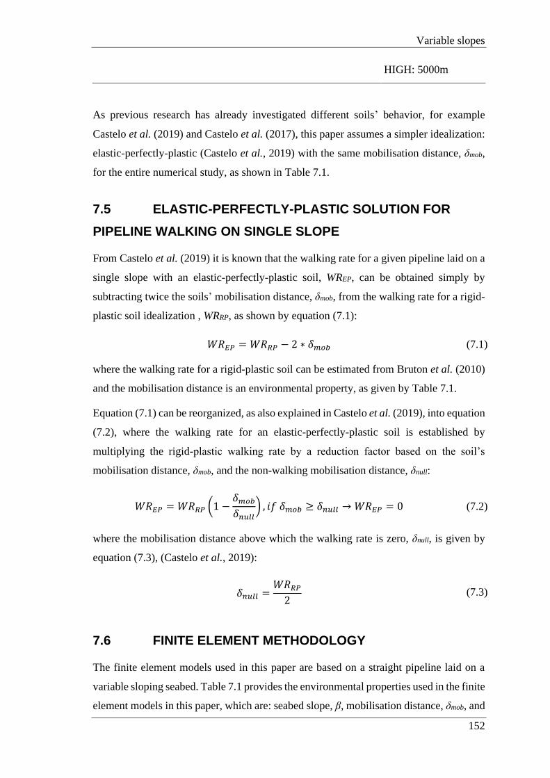
Variable slopes
152
HIGH: 5000m
As previous research has already investigated different soils’ behavior, for example
Castelo et al. (2019) and Castelo et al. (2017), this paper assumes a simpler idealization:
elastic-perfectly-plastic (Castelo et al., 2019) with the same mobilisation distance, δmob,
for the entire numerical study, as shown in Table 7.1.
7.5 ELASTIC-PERFECTLY-PLASTIC SOLUTION FOR
PIPELINE WALKING ON SINGLE SLOPE
From Castelo et al. (2019) it is known that the walking rate for a given pipeline laid on a
single slope with an elastic-perfectly-plastic soil, WREP, can be obtained simply by
subtracting twice the soils’ mobilisation distance, δmob, from the walking rate for a rigid-
plastic soil idealization , WRRP, as shown by equation (7.1):
𝑊𝑅𝐸𝑃 = 𝑊𝑅𝑅𝑃 − 2 ∗ 𝛿𝑚𝑜𝑏 (7.1)
where the walking rate for a rigid-plastic soil can be estimated from Bruton et al. (2010)
and the mobilisation distance is an environmental property, as given by Table 7.1.
Equation (7.1) can be reorganized, as also explained in Castelo et al. (2019), into equation
(7.2), where the walking rate for an elastic-perfectly-plastic soil is established by
multiplying the rigid-plastic walking rate by a reduction factor based on the soil’s
mobilisation distance, δmob, and the non-walking mobilisation distance, δnull:
𝑊𝑅𝐸𝑃 = 𝑊𝑅𝑅𝑃 (1 −𝛿𝑚𝑜𝑏𝛿𝑛𝑢𝑙𝑙
) , 𝑖𝑓 𝛿𝑚𝑜𝑏 ≥ 𝛿𝑛𝑢𝑙𝑙 → 𝑊𝑅𝐸𝑃 = 0 (7.2)
where the mobilisation distance above which the walking rate is zero, δnull, is given by
equation (7.3), (Castelo et al., 2019):
𝛿𝑛𝑢𝑙𝑙 =𝑊𝑅𝑅𝑃2
(7.3)
7.6 FINITE ELEMENT METHODOLOGY
The finite element models used in this paper are based on a straight pipeline laid on a
variable sloping seabed. Table 7.1 provides the environmental properties used in the finite
element models in this paper, which are: seabed slope, β, mobilisation distance, δmob, and

Chapter 7
153
the axial residual friction coefficient, µ; while Table 7.2 presents the operational
properties: temperature variation, ΔT, and pipe operational submerged weight, W.
The physical pipeline properties: steel outside diameter, OD, steel wall thickness, t, steel
Young’s Modulus, E, steel Poisson coefficient, ν, steel thermal expansion coefficient, α,
and the pipeline length, L, are provided in Table 7.3.
Variability was attributed to seabed slope, axial residual friction coefficient, and pipeline
length, so that the parametric study could be conducted. The pipelines were represented
by Euler Bernoulli beam elements (B33 – 3 dimensional 3 noded elements in Abaqus),
each 1m in length.
To represent the elastic-perfectly-plastic pipe-soil interaction, the soil was modelled as a
set of macro elements connected to each pipeline node, which were described as user
elements in FORTRAN.
Figure 7.3 shows a sketch of the finite element model between arbitrary nodes A and Z,
where the slope variation happens at a constant rate. It also provides information about
the boundary conditions imposed to all nodes, which can only displace along their local
longitudinal axis given the UEL reaction.
The spring-slider provided a constant stiffness between zero and a certain prescribed
displacement (mobilisation distance) and a corresponding force (according to Hooke's
law). If the displacement level exceeds the mobilisation distance, the UEL provides zero
tangent stiffness and a constant force, as per the residual plastic plateau. On reversal, the
same stiffness is considered, until the resultant force equals the residual plastic plateau.
The UEL behavior, as shown in Figure 7.4, is presented in terms of the loads normal to
the seabed alongside with the positive and negative residual plastic resistance forces, ±FR,
mobilisation distance, δmob.
The models used in this paper consider only weight and temperature (Table 7.2) as acting
loads on the pipeline. Pressure was disregarded due its marginal effect when compared
to the temperature effect.
The pipeline operational submerged weight, W, and the seabed slope angle, β, generate a
sliding component to the weight:
𝑊𝑐𝑜𝑚𝑝 = 𝑊 sin 𝛽 (7.4)
Operational cycling considered the prescribed temperature variation, as per Table 7.2,

Variable slopes
154
from the starting to the end model nodes, i.e. over the entire pipeline length, without any
intermediate temperature load case.
7.7 RANGE OF PARAMETRIC STUDIES
The present numerical study verifies the applicability of single slope pipeline walking
solutions to variable slopes topography, by using an average seabed slope, βave, applied
to the entire pipeline length, based on the environmental properties faced by a specific
pipeline route.
The numerical study uses the values provided in Table 7.1, Table 7.2 and Table 7.3 as
previously explained.
Finally, to investigate the slope variability impact on the pipeline walking phenomenon,
four different topographies were selected to be investigated. These are:
• Dual slope – convex;
• Dual slope – concave;
• Triple slope – flat-slope-flat;
• Triple slope – slope-flat-slope.
7.7.1 Dual slope – convex
Some pipelines are employed in regions where they face two different slopes with a steep
start, near the initial pipeline kilometer post, KP, and a smaller slope near the final KP.
This topography is illustrated by Figure 7.5.
These pipelines may face different angles along different stretches of their length. Hence,
these aspects were accounted for the numerical study through different models, whose
properties can be seen in Table 7.4 for gentle (models 01 – 13) and extreme (models 14
– 26) angles.
Table 7.4: Dual slope convex model properties
Model Property Values
μ L1 (m) L2 (m) β1 (°) β2 (°)
01 0.5 1500 1500 3 1
02 0.7 1500 1500 3 1
03 0.9 1500 1500 3 1
04 0.5 2000 2000 3 1

Chapter 7
155
05 0.7 2000 2000 3 1
06 0.9 2000 2000 3 1
07 0.5 2500 2500 3 1
08 0.7 2500 2500 3 1
09 0.9 2500 2500 3 1
10 0.9 2500 2500 4 2
11 0.9 1500 1500 4 2
12 0.9 2000 2000 4 2
13 0.7 2000 2000 4 2
14 0.9 2500 2500 6 4
15 0.9 2000 3000 7 3
16 0.9 1500 3500 8 2
17 0.9 1000 4000 9 1
18 0.9 1000 4000 10 0
19 0.9 2000 2000 7 3
20 0.9 2000 2000 7 2
21 0.9 2000 2000 7 1
22 0.9 2000 2000 6 3
23 0.9 1000 2000 7 3
24 0.9 1000 2000 8 2
25 0.9 2000 1000 7 1
26 0.9 2000 1000 6 1
7.7.2 Dual slope – concave
In other regions, pipelines face a small angle near the initial KP and a steeper slope near
the final KP. This shape is illustrated by Figure 7.5.
Table 7.5 presents the parameters considered for the numerical study, considering gentle
slopes (models 27 – 39) and extreme slopes (models 40 – 52).
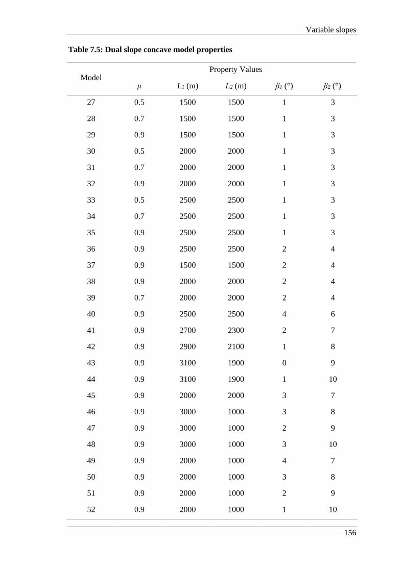
Variable slopes
156
Table 7.5: Dual slope concave model properties
Model Property Values
μ L1 (m) L2 (m) β1 (°) β2 (°)
27 0.5 1500 1500 1 3
28 0.7 1500 1500 1 3
29 0.9 1500 1500 1 3
30 0.5 2000 2000 1 3
31 0.7 2000 2000 1 3
32 0.9 2000 2000 1 3
33 0.5 2500 2500 1 3
34 0.7 2500 2500 1 3
35 0.9 2500 2500 1 3
36 0.9 2500 2500 2 4
37 0.9 1500 1500 2 4
38 0.9 2000 2000 2 4
39 0.7 2000 2000 2 4
40 0.9 2500 2500 4 6
41 0.9 2700 2300 2 7
42 0.9 2900 2100 1 8
43 0.9 3100 1900 0 9
44 0.9 3100 1900 1 10
45 0.9 2000 2000 3 7
46 0.9 3000 1000 3 8
47 0.9 3000 1000 2 9
48 0.9 3000 1000 3 10
49 0.9 2000 1000 4 7
50 0.9 2000 1000 3 8
51 0.9 2000 1000 2 9
52 0.9 2000 1000 1 10
Chapter 7
157
7.7.3 Triple slope – flat-slope-flat
Alternatively, pipelines may also be employed in regions where they cross a flat region
before facing a route slope and return to a flat area near their final kilometer post, KP.
This type of topography is illustrated in Figure 7.6.
These pipelines may face different angles. Then, these aspects were considered for the
numerical study through different models, whose properties are shown in Table 7.6 for
gentle angles (models 53 – 65) and extreme angles (models 66 – 78).
Table 7.6: Triple slope flat-slope-flat model properties
Model Property Values
μ L1 (m) L2 (m) L3 (m) β1 (°) β2 (°) β3 (°)
53 0.5 1500 2000 1500 0 3 0
54 0.5 1000 3000 1000 0 3 0
55 0.5 500 4000 500 0 3 0
56 0.7 500 4000 500 0 3 0
57 0.5 1500 1000 1500 0 4 0
58 0.5 1000 2000 1000 0 4 0
59 0.5 500 3000 500 0 4 0
60 0.7 500 3000 500 0 4 0
61 0.5 1000 1000 1000 0 3 0
62 0.5 500 2000 500 0 3 0
63 0.7 500 2000 500 0 3 0
64 0.5 500 2000 500 0 5 0
65 0.5 500 4000 500 0 2 0
66 0.9 1500 2000 1500 0 10 0
67 0.9 1000 3000 1000 0 8 0
68 0.9 500 4000 500 0 6 0
69 0.7 1000 3000 1000 0 6 0
70 0.7 1750 500 1750 0 10 0
71 0.9 1500 1000 1500 0 8 0

Variable slopes
158
72 0.9 1250 1500 1250 0 8 0
73 0.9 1500 1000 1500 0 10 0
74 0.5 1000 1000 1000 0 6 0
75 0.7 1000 1000 1000 0 6 0
76 0.7 1300 400 1300 0 10 0
77 0.7 1200 600 1200 0 10 0
78 0.9 1200 600 1200 0 10 0
7.7.4 Triple slope – flat-slope-flat
Other regions may require that pipelines cross a sloped area before facing a flat area and
then cross another slope near their final KP. This shape is schematically shown in Figure
7.6.
Table 7.7 presents the parameters considered for the numerical study for gentle angles
(models 79 – 91) and extreme angles (models 92 – 104).
Table 7.7: Triple slope slope-flat-slope model properties
Model Property Values
μ L1 (m) L2 (m) L3 (m) β1 (°) β2 (°) β3 (°)
79 0.5 1500 2000 1500 3 0 3
80 0.5 1000 3000 1000 3 0 3
81 0.5 500 4000 500 3 0 3
82 0.7 500 4000 500 3 0 3
83 0.7 1500 1000 1500 4 0 4
84 0.7 1000 2000 1000 4 0 4
85 0.5 500 3000 500 4 0 4
86 0.7 500 3000 500 4 0 4
87 0.5 1000 1000 1000 3 0 3
88 0.5 500 2000 500 3 0 3
89 0.7 500 2000 500 3 0 3
90 0.7 500 2000 500 5 0 5

Chapter 7
159
91 0.5 500 4000 500 2 0 2
92 0.9 500 4000 500 10 0 10
93 0.9 750 3500 750 9 0 9
94 0.9 1000 3000 1000 8 0 8
95 0.9 500 4000 500 8 0 8
96 0.9 1750 500 1750 5 0 5
97 0.5 500 3000 500 5 0 5
98 0.7 500 3000 500 5 0 5
99 0.9 500 3000 500 5 0 5
100 0.9 500 2000 500 6 0 6
101 0.9 1000 1000 1000 6 0 6
102 0.9 500 2000 500 7 0 7
103 0.9 500 2000 500 9 0 9
104 0.9 1000 1000 1000 7 0 7
7.8 FINITE ELEMENT MODEL RESULTS
Table 7.8 and Table 7.9 show the following properties for the dual slope cases (convex
and concave, respectively):
• Residual axial friction coefficient, μ;
• Total length of the pipeline, LTotal;
• Average seabed slope angle, βave;
• Calculated walking rate, WRCalc, as per Castelo et al. (2019); and,
• Finite element model observed walking rate, WRFEM.
Table 7.8: Dual slope – Convex model results
Model
Properties Results
μ LTotal (m) βave (°) WRCalc
(m/cycle)
WRFEM
(m/cycle)
01 0.5 3000 2.0 0.106596 0.105418
02 0.7 3000 2.0 0.035611 0.035033
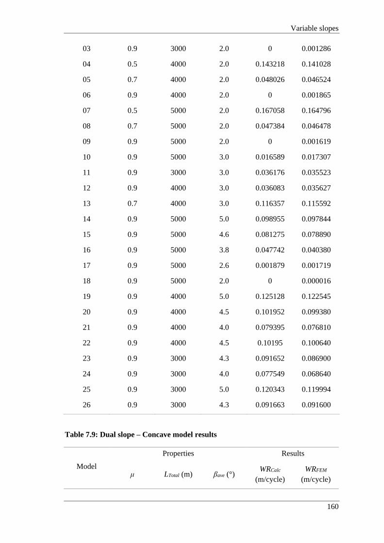
Variable slopes
160
03 0.9 3000 2.0 0 0.001286
04 0.5 4000 2.0 0.143218 0.141028
05 0.7 4000 2.0 0.048026 0.046524
06 0.9 4000 2.0 0 0.001865
07 0.5 5000 2.0 0.167058 0.164796
08 0.7 5000 2.0 0.047384 0.046478
09 0.9 5000 2.0 0 0.001619
10 0.9 5000 3.0 0.016589 0.017307
11 0.9 3000 3.0 0.036176 0.035523
12 0.9 4000 3.0 0.036083 0.035627
13 0.7 4000 3.0 0.116357 0.115592
14 0.9 5000 5.0 0.098955 0.097844
15 0.9 5000 4.6 0.081275 0.078890
16 0.9 5000 3.8 0.047742 0.040380
17 0.9 5000 2.6 0.001879 0.001719
18 0.9 5000 2.0 0 0.000016
19 0.9 4000 5.0 0.125128 0.122545
20 0.9 4000 4.5 0.101952 0.099380
21 0.9 4000 4.0 0.079395 0.076810
22 0.9 4000 4.5 0.10195 0.100640
23 0.9 3000 4.3 0.091652 0.086900
24 0.9 3000 4.0 0.077549 0.068640
25 0.9 3000 5.0 0.120343 0.119994
26 0.9 3000 4.3 0.091663 0.091600
Table 7.9: Dual slope – Concave model results
Model
Properties Results
μ LTotal (m) βave (°) WRCalc
(m/cycle)
WRFEM
(m/cycle)

Chapter 7
161
27 0.5 3000 2.0 0.106580 0.104538
28 0.7 3000 2.0 0.035601 0.034397
29 0.9 3000 2.0 0 0.001184
30 0.5 4000 2.0 0.143204 0.141432
31 0.7 4000 2.0 0.048018 0.046693
32 0.9 4000 2.0 0 0.001749
33 0.5 5000 2.0 0.167045 0.164354
34 0.7 5000 2.0 0.047377 0.046532
35 0.9 5000 2.0 0 0.000996
36 0.9 5000 3.0 0.016585 0.017212
37 0.9 3000 3.0 0.036176 0.035701
38 0.9 4000 3.0 0.036083 0.035567
39 0.7 4000 3.0 0.116357 0.115395
40 0.9 5000 5.0 0.098950 0.097864
41 0.9 5000 4.3 0.068417 0.068170
42 0.9 5000 3.9 0.053435 0.053310
43 0.9 5000 3.4 0.032646 0.032755
44 0.9 5000 4.4 0.073517 0.074023
45 0.9 4000 5.0 0.125116 0.122890
46 0.9 4000 4.3 0.090586 0.090960
47 0.9 4000 3.8 0.068331 0.068488
48 0.9 4000 4.8 0.113451 0.113523
49 0.9 3000 5.0 0.120332 0.119374
50 0.9 3000 4.7 0.105910 0.105470
51 0.9 3000 4.3 0.091649 0.091810
52 0.9 3000 4.0 0.077546 0.077145
With the same table structure, Table 7.10 and Table 7.11 present the results for flat-slope-
flat and slope-flat-slope geometries, respectively, accounting for gentle and extreme
angles.

Variable slopes
162
Table 7.10: Triple slope flat-slope-flat model results
Model
Properties Results
μ LTotal (m) βave (°) WRCalc
(m/cycle)
WRFEM
(m/cycle)
53 0.5 5000 1.2 0.065240 0.059084
54 0.5 5000 1.8 0.141220 0.133603
55 0.5 5000 2.4 0.219433 0.210500
56 0.7 5000 2.4 0.074987 0.071869
57 0.5 4000 1.0 0.029641 0.027041
58 0.5 4000 2.0 0.143211 0.133256
59 0.5 4000 3.0 0.260856 0.252641
60 0.7 4000 3.0 0.116361 0.110550
61 0.5 3000 1.0 0.012180 0.010683
62 0.5 3000 2.0 0.106580 0.101793
63 0.7 3000 2.0 0.035601 0.034377
64 0.5 3000 3.3 0.236102 0.230289
65 0.5 5000 1.6 0.115653 0.110969
66 0.9 5000 4.0 0.055908 0.042230
67 0.9 5000 4.8 0.090046 0.077470
68 0.9 5000 4.8 0.090042 0.079980
69 0.7 5000 3.6 0.162266 0.159180
70 0.7 4000 1.3 0 0.000194
71 0.9 4000 2.0 0 0.000330
72 0.9 4000 3.0 0.036096 0.035460
73 0.9 4000 2.5 0.015313 0.010670
74 0.5 3000 2.0 0.106604 0.104897
75 0.7 3000 2.0 0.035616 0.031720
76 0.7 3000 1.3 0 0.000037
77 0.7 3000 2.0 0.035636 0.026360

Chapter 7
163
78 0.9 3000 2.0 0 0.000121
Table 7.11: Triple slope slope-flat-slope model results
Model
Properties Results
μ LTotal (m) βave (°) WRCalc
(m/cycle)
WRFEM
(m/cycle)
79 0.5 5000 1.8 0.141208 0.133386
80 0.5 5000 1.2 0.065266 0.057494
81 0.5 5000 0.6 0 0.000491
82 0.7 5000 0.6 0 0.000090
83 0.7 4000 3.0 0.116343 0.111040
84 0.7 4000 2.0 0.048005 0.044223
85 0.5 4000 1.0 0.029614 0.024999
86 0.7 4000 1.0 0 0.000143
87 0.5 3000 2.0 0.106556 0.100635
88 0.5 3000 1.0 0.012156 0.008746
89 0.7 3000 1.0 0 0.000070
90 0.7 3000 1.7 0.015872 0.011900
91 0.5 5000 0.4 0 0.000079
92 0.9 5000 2.0 0 0.000111
93 0.9 5000 2.7 0.005532 0.003600
94 0.9 5000 3.2 0.024151 0.023130
95 0.9 5000 1.6 0 0.000031
96 0.9 4000 4.4 0.096236 0.090840
97 0.5 4000 1.3 0.057630 0.049700
98 0.7 4000 1.3 0 0.000264
99 0.9 4000 1.3 0 0.000013
100 0.9 3000 2.0 0 0.000143
101 0.9 3000 4.0 0.077528 0.070430

Variable slopes
164
102 0.9 3000 2.3 0.009347 0.004670
103 0.9 3000 3.0 0.036196 0.035010
104 0.9 3000 4.7 0.105883 0.101833
In general terms, when accounting for all models’ results, the overall percentage error
generated by the solution proposed by this paper is 6.442% only, which is a marginal
deviation.
Figure 7.7 presents the walking rate results from the numerical solutions (finite element
models) plotted against the values calculated by equation (7.1). Cross markers represent
the dual slope convex shape, while square markers represent dual slope concave shape.
Circle markers represent flat-slope-flat shape, whilst triangle markers stand for slope-
flat-slope shapes. The colors gray and black represent gentle and extreme angles,
respectively.
As can be seen in Figure 7.7 and as previously explained, the deviation found between
the analytical formulation and the finite element models can be classified as marginal.
Therefore, the accuracy and applicability from the proposed methodology can be
regarded as appropriate.
7.9 CONCLUSIONS & FINAL REMARKS
This paper provides the technical confirmation to the available methods about pipeline
walking on a variable slopes’ topography. It shows that the analytical expressions
currently available in the literature can be applied with an average slope value; and,
proves so, by an extensive benchmark against finite element analyses test (focused solely
on seabed slope variability).
This paper also proves that emerging research on pipe-soil interaction variability can
properly solve gravity-driven downslope pipeline walking problems with slope
variability.
Different slopes and properties of slope variability have been considered in this paper;
while it also checked how currently available solutions (single-slope and rigid-plastic
pipe-soil interaction) could be adapted to allow for slope and pipe-soil interaction
variabilities. Therefore, this paper resolves how currently available solutions must be
adjusted to allow for slope variability and realistic pipe-soil interactions.

Chapter 7
165
In conclusion, the findings of this paper can be used to assess the pipeline walking
behaviors for a variable-slope laid pipeline while also accounting for realistic pipe-soil
interactions.
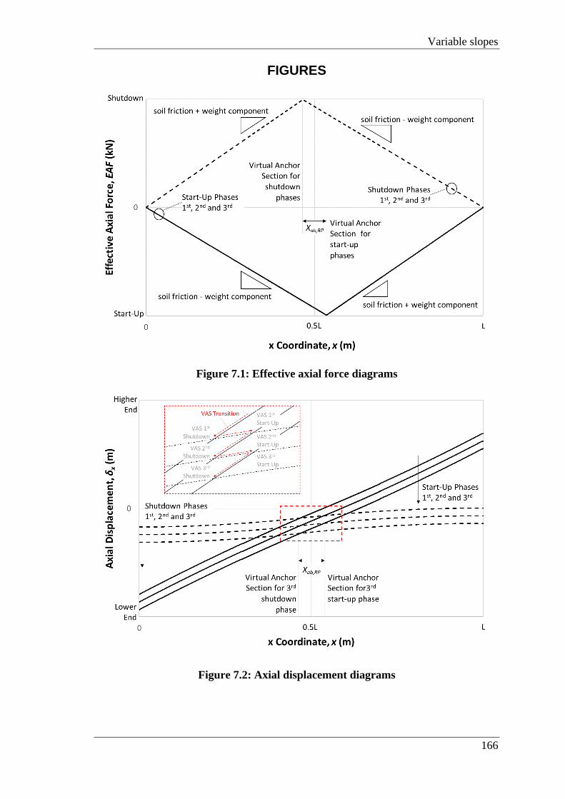
Variable slopes
166
FIGURES
Figure 7.1: Effective axial force diagrams
Figure 7.2: Axial displacement diagrams

Chapter 7
167
Figure 7.3: Finite element model sketch
Figure 7.4: User element behavior

Variable slopes
168
Figure 7.5: Dual slope general shapes
Figure 7.6: Triple slope general shapes
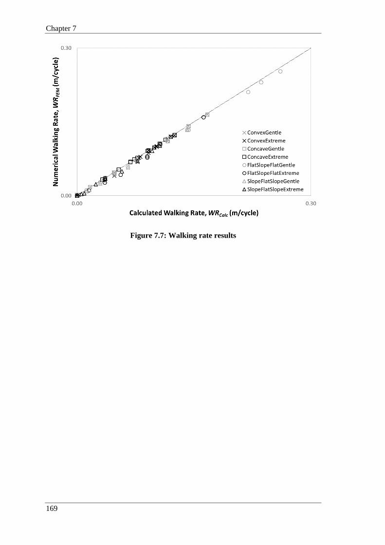
Chapter 7
169
Figure 7.7: Walking rate results

Concluding remarks
170
CHAPTER 8. CONCLUDING REMARKS
Chapter context: In the following sections are listed the principal findings and their
contributions on the assessment of downslope pipeline walking for future engineering
studies. Recommendations for further research are also presented in this chapter.

Chapter 8
171
8.1 PRINCIPAL FINDINGS AND CONTRIBUTIONS
This thesis improves the understanding about downslope pipeline walking and soil
variables by accomplishing the research goals listed in Chapter 1. As presented in Section
1.2, the goals of this thesis were fulfilled delivering four major contributions:
1. Revision of the analytical equations;
2. Interpretation of the changes in walking behaviour;
3. Expansion to any pipe-soil interaction;
4. Confirmation of applicability on variable slopes.
8.1.1 Pipe-soil interaction models
This thesis starts by reviewing the available literature on the subject, alongside with other
engineering topics that are associated to the methods of research. It shows how the current
solutions idealise the realistic pipe-soil interaction models as a rigid-plastic model.
The following subheadings provide some details on how such pipe-soil interaction
models were found to interfere on the downslope pipeline walking pattern. For the
analytical methodology updates, please refer to Section 8.1.3, where the new analytical
assessment of downslope pipeline walking is summarised.
Elastic-perfectly-plastic
In Chapter 3, the research starts by analytically investigating the elastic-perfectly-plastic
pipe-soil interaction model and its impacts on the downslope walking behaviour. In this
chapter a detailed revision of the analytical formulation is presented, which enhances the
interpretations on the walking behaviour.
The analytical investigation found that the distance between stationary points (initially
referred to as “virtual anchor sections”) has a major influence in the walking behaviour;
and, the definition primarily given by Carr et al. (2006) needed to be updated. The
findings of Chapter 3 show why the “virtual anchor sections” should be substituted by
the “stationary points” and how the distance between stationary points can be obtained
by adjusting the previously available analytical solution.
The chapter then presents a methodology allowing current analytical solutions (Carr et
al., 2006) to account for elastic-perfectly-plastic pipe-soil interaction in a similar fashion
as it was initially proposed to the distance between stationary points.

Concluding remarks
172
Non-linear elastic-plastic
Chapter 4 develops the analytical investigation initially presented in Chapter 3 by
considering non-linear elastic-plastic pipe-soil interaction model. Another detailed
revision of the analytical formulation is presented enhancing the understandings on the
walking behaviour.
It was found that the same influence was generated by the distance between stationary
points; and similar updates were required for the non-linear elastic-plastic pipe-soil
interaction model. The chapter also establishes how a non-linear elastic-plastic pipe-soil
interaction can be satisfactorily approximated to an elastic-perfectly-plastic pipe-soil
interaction model. It also drives attention to the non-walking behaviour that was found
from some simulations and provides the necessary justifications for the non-walking
behaviour.
The chapter conclude that with the proper adjustments, the currently used analytical
solutions allow for the non-linear elastic-plastic pipe-soil interaction to be analytically
assessed
Tri-linear with a peak
Based on Chapters 3 and 4 outcomes, Chapter 5 skips the analytical investigation and
starts from the numerical modelling to prove that similar adjustments could be done to
the current analytical solutions.
Aligned with the previous findings, the distance between stationary points has also been
found to generate changes in walking patterns; even though the pipe-soil interaction
presents a peak. The chapter clarifies that the referred peak can be ignored since its impact
has a marginal and negligible effect on the downslope pipeline walking phenomenon.
The chapter shows how the adjustments to the analytical solutions are done for tri-linear
soils with a peak, which perfectly aligns with the previous findings.
Non-linear with a peak
Chapter 6 findings show the necessary adjustments for the application of the new
analytical assessments of downslope pipeline walking on non-linear soils with a peak. It
clarifies that different shapes of non-linearity generate different influences in the walking
behaviour, i.e. the greater the pipe-soil interaction unload-reload area, AUnload-Reload, the
greater the over conservatism implied by the rigid-plastic solutions.
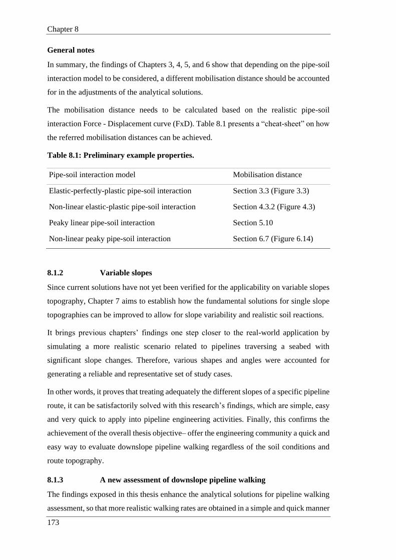
Chapter 8
173
General notes
In summary, the findings of Chapters 3, 4, 5, and 6 show that depending on the pipe-soil
interaction model to be considered, a different mobilisation distance should be accounted
for in the adjustments of the analytical solutions.
The mobilisation distance needs to be calculated based on the realistic pipe-soil
interaction Force - Displacement curve (FxD). Table 8.1 presents a “cheat-sheet” on how
the referred mobilisation distances can be achieved.
Table 8.1: Preliminary example properties.
Pipe-soil interaction model Mobilisation distance
Elastic-perfectly-plastic pipe-soil interaction Section 3.3 (Figure 3.3)
Non-linear elastic-plastic pipe-soil interaction Section 4.3.2 (Figure 4.3)
Peaky linear pipe-soil interaction Section 5.10
Non-linear peaky pipe-soil interaction Section 6.7 (Figure 6.14)
8.1.2 Variable slopes
Since current solutions have not yet been verified for the applicability on variable slopes
topography, Chapter 7 aims to establish how the fundamental solutions for single slope
topographies can be improved to allow for slope variability and realistic soil reactions.
It brings previous chapters’ findings one step closer to the real-world application by
simulating a more realistic scenario related to pipelines traversing a seabed with
significant slope changes. Therefore, various shapes and angles were accounted for
generating a reliable and representative set of study cases.
In other words, it proves that treating adequately the different slopes of a specific pipeline
route, it can be satisfactorily solved with this research’s findings, which are simple, easy
and very quick to apply into pipeline engineering activities. Finally, this confirms the
achievement of the overall thesis objective– offer the engineering community a quick and
easy way to evaluate downslope pipeline walking regardless of the soil conditions and
route topography.
8.1.3 A new assessment of downslope pipeline walking
The findings exposed in this thesis enhance the analytical solutions for pipeline walking
assessment, so that more realistic walking rates are obtained in a simple and quick manner

Concluding remarks
174
accounting for realistic pipe-soil interaction properties. The new analytical results are
more accurate than the previous formulation because it reduces the conservativeness
implied by the rigid-plastic pipe-soil calculations. It eliminates the overestimation of
walking based on the realistic pipe-soil interaction, as shown in Chapters 3 to 7; and, the
comparison between the new analytical and finite element results. This improvement in
accuracy also eliminates the need for finite element modelling.
In conclusion, the findings of this research can be summarised as:
𝑊𝑅 = 𝑊𝑅𝑅𝑃 ∗ (1 −𝛿𝑚𝑜𝑏𝛿𝑛𝑢𝑙𝑙
) , 𝑖𝑓 𝛿𝑚𝑜𝑏 ≥ 𝛿𝑛𝑢𝑙𝑙 → 𝑊𝑅 = 0 (8.1)
where WR stands for the walking rate, RP for rigid-plastic, δmob for the mobilisation
distance and δnull for the non-walking mobilisation distance.
The findings of this thesis also clarify that the mobilisation distance, δmob, to be accounted
for in equation (8.1), should be obtained using equation (8.2):
𝛿𝑚𝑜𝑏 =𝐴𝑈𝑛𝑙𝑜𝑎𝑑−𝑅𝑒𝑙𝑜𝑎𝑑
𝛥𝐹𝑅 (8.2)
where AUnload-Reload is the unload-reload area, and ΔFR is the variation in residual friction
as it is referenced prior to Table 8.1 by the realistic pipe-soil interaction Force -
Displacement curve (FxD).
And the non-walking mobilisation distance, δnull, should be obtained using equation (8.3):
𝛿𝑛𝑢𝑙𝑙 =𝑊𝑅𝑅𝑃2
(8.3)
The rigid-plastic walking rate can be calculated, as per Bruton et al. (2010):
𝑊𝑅𝑅𝑃 =[|𝛥𝑃| +𝑊𝐿|sin 𝛽| −𝑊𝐿𝜇 cos 𝛽]𝐿 tan 𝛽
𝐸𝐴𝜇 (8.4)
while, W stands for the pipeline operational submerged weight, L for pipeline physical
length, β for seabed slope angle, µ for the soil axial residual friction coefficient, E for the
steel Young’s modulus and A for the pipeline steel cross sectional area. And, ΔP is the
change in fully constrained force, as per Carr et al. (2003).
Therefore, it can be concluded that, for any pipe-soil interaction condition, it is now
available a simple and direct analytical solution, which makes quicker and more precise
the assessment of a pipeline in regards of downslope walking issues.
Chapter 8
175
8.2 FURTHER RESEARCH RECOMMENDATIONS
This research project resulted into several new findings concerning the downslope
pipeline walking phenomenon. The PhD candidate and his supervisors believe that
similar research processes could be applied into other problems, but which were beyond
the scope of the present work. These are:
1. Sustained tension, thermal transients and multiphase flow pipeline walking. The
suggested research here is related to the same phenomenon but driven by other
causes. These are the three other drivers of pipeline walking (Bruton et al., 2010)
and a similar strategy could be used in order to review the available analytical
expressions and then more robust analytical formulation becomes accessible for
future industry and academic activities.
2. Interaction between pipeline walking and lateral buckling. The interaction
between pipeline walking and lateral buckling has been an issue treated in a case
by case strategy; although it has been in the spotlight for a while. Lateral buckling
itself is a major issue, which may have its consequences potentiated by the
influence of pipeline walking. If not properly designed, lateral buckling may
cause serious damages to pipeline.

References
176
REFERENCES
Azevedo, F., Haverroth, G. and Genaio, M. (2018) ‘Offshore Export Gas Pipeline in Pre
Salt Santos Basin - Historic, Optimizations and Lessons Learned’, in Proceedings of the
Offshore Technology Conference. Houston, pp. 2117–2125. doi: 10.4043/28965-ms.
Ballard, J.-C. and Falepin, H. (2009) ‘Towards More Aadvanced Pipe-Soil Interaction
Models in Finite Element Pipeline Analysis’, in Proceedings of the SUT Annual
Conference 2009.
Bruton, D. et al. (2008) ‘Pipe-Soil Interaction with Flowlines During Lateral Buckling
and Pipeline Walking - The SAFEBUCK JIP’, in Proceedings of the Offshore Pipeline
Technology Conference. doi: 10.4043/19589-MS.
Bruton, D. et al. (2009) ‘Techniques for the Assessment of Pipe-Soil Interaction Forces
for Future Deepwater Developments’, in Proceedings of the Offshore Technology
Conference. doi: 10.4043/20096-MS.
Bruton, D. and Carr, M. (2011a) ‘Lateral Buckling and Pipeline Walking - Overview of
the SAFEBUCK JIP’, in Proceedings of the Subsea Australasia Conference 2011.
Bruton, D. and Carr, M. (2011b) ‘Overview of the SAFEBUCK JIP’, in Proceedings of
the Offshore Pipeline Technology Conference. doi: 10.4043/21671-MS.
Bruton, D., Carr, M. and White, D. (2007) ‘The Influence of Pipe-Soil Interaction on
Lateral Buckling and Walking of Pipelines - the SAFEBUCK JIP’, in Proceedings of the
International Conference on Offshore Site Investigation and Geotechnics.
Bruton, D., Sinclair, F. and Carr, M. (2010) ‘Lessons Learned from Observing Walking
of Pipelines with Lateral Buckles, Including New Driving Mechanisms and Updated
Analysis Models’, in Proceedings of the Offshore Technology Conference. doi:
10.4043/20750-MS.
Carneiro, D. et al. (2017) ‘Active Pressure of Rock Berms on Pipelines’, in Proceedings
of the 8th International Conference on Offshore Site Investigation Geotechnics.
Carneiro, D. and Castelo, A. (2011) ‘Walking Analyses of HP/ HT Pipelines with Sliding
End Structures Using Different FE Models’, in Proceedings of the Rio Pipeline
Conference and Exposition 2011.
Carneiro, D. and Murphy, D. (2011) ‘Simple Numerical Models for Pipeline Walking
Accounting for Mitigation and Complex Soil Response’, in Proceedings of the ASME
2011 30th International Conference on Ocean, Offshore and Arctic Engineering.
Carr, M., Bruton, D. and Leslie, D. (2003) ‘Lateral Buckling and Pipeline Walking, a
Challenge for Hot Pipelines’, in Proceedings of the Offshore Pipeline Technology
Conference.
Carr, M., Sinclair, F. and Bruton, D. (2006) ‘Pipeline Walking - Understanding the Field
Layout Challenges and Analytical Solutions Developed for the Safebuck JIP’, in
Proceedings of the Offshore Technology Conference. doi: 10.2118/120022-PA.

References
177
Castelo, A., White, D. and Tian, Y. (2017) ‘Solving Downslope Pipeline Walking on
Non-Linear Soil with Brittle Peak Strength and Strain Softening’, in Proceedings of the
ASME 2017 36th International Conference on Ocean, Offshore and Arctic Engineering.
Trondheim, Norway, pp. 1–13.
Castelo, A., White, D. and Tian, Y. (2019) ‘Simple Solutions for Downslope Pipeline
Walking on Elastic-Perfectly-Plastic Soils’, Ocean Engineering. Elsevier Ltd, 172, pp.
671–683. doi: 10.1016/j.oceaneng.2018.11.037.
Castelo, A., White, D. and Tian, Y. (no date a) ‘Solutions for Downslope Pipeline
Walking on Peaky Tri-Linear Soils’, Offshore Mechanics and Arctic Engineering.
Castelo, A., White, D. and Tian, Y. (no date b) ‘Solving Downslope Pipeline Walking on
Non-Linear Elastic-Plastic Soils’, Marine Structures.
Castelo, A., White, D. and Tian, Y. (no date c) 'Gravity-driven pipeline walking on
slopes’, International Journal of Offshore and Polar Engineering.
Chan, J. and Matlock, H. (1973) ‘A Discrete-Element Method for Transverse Vibrations
of Beam Columns Resting on Linearly Elastic or Inelastic Supports’, in Proceedings of
the Offshore Technology Conference.
Charnaux, C. et al. (2015) ‘Design and Installation Challenges of P-55 Gas and Oil
Export Pipelines Project’, in Proceedings of the Rio Pipeline Conference and Exposition
2015.
DASSAULT SYSTÈMES (2014) ‘Abaqus 6.14 Analysis User’s Manual’. Providence,
RI, USA: Dassault Systèmes Simulia Corporation.
DNVGL (2017a) DNVGL-RP-F114: Pipe-Soil Interaction for Submarine Pipelines.
DNVGL (2017b) DNVGL-ST-F101: Submarine Pipeline Systems.
DNVGL (2018) DNVGL-RP-F110: Global Buckling of Submarine Pipelines.
Frankenmolen, S. et al. (2017) ‘Pipe-Clamping Mattress to Stop Flowline Walking’, in
Proceedings of the Offshore Technology Conference. doi: 10.4043/27815-MS.
Frazer, I., Perinet, D. and Rochereau, M. (2007) ‘Pressure and Temperature Induced
Movements of Deep Water Pipelines and Methods to Mitigate Their Affects’, in
Proceedings of the Rio Pipeline Conference and Exposition 2007.
Halliday, D., Resnick, R. and Walker, J. (2010) Fundamentals of Physics. 9th ed.
Jefferson City: Wiley.
Hill, A. et al. (2012) ‘A New Framework for Axial Pipe-Soil Resistance, Illustrated by a
Range of Marine Clay Datasets’, in Proceedings of the International Conference on
Offshore Site Investigation and Geotechnics.
Hill, A. and Jacob, H. (2008) ‘In-Situ Measurement of Pipe-Soil Interaction in Deep
Water’, in Proceedings of the Offshore Technology Conference. doi: 10.4043/19528-MS.

References
178
Hobbs, R. (1984) ‘In‐Service Buckling of Heated Pipelines’, Journal of Transportation
Engineering, 110(2), pp. 175–189. doi: 10.1061/(ASCE)0733-947X(1984)110:2(175).
Jayson, D. et al. (2008) ‘Greater Plutonio Project - Subsea Flowline Design and
Performance’, in Proceedings of the Offshore Pipeline Technology Conference.
Konuk, I. (1998). 'Expansion of Pipelines Under Cyclic Operational Conditions:
Formulation of Problem and Development of Solution Algorithm’, in Proceeding of the
ASME 1998 17th International Conference on Ocean, Offshore and Arctic Engineering.
Kumar, A. and Mcshane, B. (2009) ‘Global Buckling and Axial Stability for HP/HT
Flowlines’, in Proceedings of the Offshore Technology Conference.
Kyriakides, S. and Corona, E. (2007) Mechanics of Offhsore Pipelines. 1st ed. Oxford:
Elsevier Science.
Leckie, S. et al. (2016) ‘Sedimentation-Induced Burial of Subsea Pipelines: Observations
from Field Data and Laboratory Experiments’, Journal of Coastal Engineering, 114, pp.
137–158. doi: 10.1016/j.coastaleng.2016.04.017.
Palmer, A. and Baldry, J. (1974) ‘Lateral Buckling of Axially Constrained Pipelines’,
Journal of Petroleum Technology, 26(11), pp. 1283–1284.
Palmer, A. and Croasdale, K. (2012) Arctic Offshore Engineering. 1st ed. Singapore:
World Scientific.
Palmer, A. and King, R. (2008) Subsea Pipeline Engineering. 2nd ed. Tulsa: Pennwell
Books. doi: 621.643.
Perinet, D. and Simon, J. (2011) ‘Lateral Buckling and Pipeline Walking Mitigation in
Deep Water’, in Proceedings of the Offshore Technology Conference. doi:
10.4043/21803-MS.
Randolph, M. (1977) A Theoretical Study of the Performance of Piles. University of
Cambridge.
Randolph, M. and White, D. (2008) ‘Pipeline Embedment in Deep Water: Processes and
Quantitative Assessment’, in Proceedings of the Offshore Technology Conference. doi:
10.4043/19128-MS.
Roberts, G. et al. (2018) ‘Flexible Flowline Walking Tendency on Seabed with
Longitudinal Undulations and Transverse Gradients’, in Proceedings of the ASME 2018
37th International Conference on Ocean, Offshore and Arctic Engineering.
Rong, H. et al. (2009) ‘Evaluation and Mitigation of Axial Walking with a Focus on Deep
Water Flowlines’, in Proceedings of the Offshore Technology Conference.
Sinclair, F. et al. (2009) ‘Design Challenges and Experience with Controlled Lateral
Buckle Initiation Methods’, in Proceedings of the ASME 2009 28th International
Conference on Ocean, Offshore and Arctic Engineering. doi: 10.1115/OMAE2009-
79434.
References
179
Smith, V. and White, D. (2014) ‘Volumetric Hardening in Axial Pipe Soil Interaction’,
in Proceedings of the Offshore Technology Conference Asia. doi: 10.4043/24856-MS.
Solano, R. et al. (2009) ‘A Fast-Track Preliminary Thermo-Mechanical Design of Oil
Export Pipelines from P-56 Platform’, in Proceedings of the Rio Pipeline Conference and
Exposition 2009.
Solano, R. et al. (2014) ‘Lateral Buckling and Walking Design of a Pipeline Subjected to
a High Number of Operational Cycles on Very Uneven Seabed’, in Proceedings of the
ASME 2014 33rd International Conference on Ocean, Offshore and Arctic Engineering.
Thompson, H. et al. (2009) ‘Tahiti Flowline Expansion Control System’, in Proceedings
of the Offshore Technology Conference. doi: 10.4043/19858-MS.
Tian, Y. and Cassidy, M. (2008) ‘Explicit and implicit integration algorithms for an
elastoplastic pipe-soil interaction macroelement model’, in 27th International
Conference on Offshore Mechanics and Arctic Engineering.
Tornes, K. et al. (2000) ‘Axial Creeping of High Temperature Flowlines Caused by Soil
Ratcheting’, in Proceedings of the ETCE/ OMAE Joint Conference, Energy for the New
Millennium.
Watson, R., Bruton, D. and Sinclair, F. (2010) ‘Influence of Multiphase Flow on Global
Displacement of Deepwater Pipelines – in Design and Operation’, in Proceedings of the
5th International Offshore Pipeline Forum.
Watson, R., Sinclair, F. and Bruton, D. (2011) ‘SAFEBUCK JIP: Operational Integrity
of Deepwater Flowlines’, in Proceedings of the Offshore Technology Conference. doi:
10.4043/21724-MS.
White, D. (2011) ‘Pipeline and Riser Geotechnics’, in Offshore Geotechnical
Engineering. 1st ed. Milton Park, Oxon: Spoon Press, pp. 404–443.
White, D. et al. (2011) ‘SAFEBUCK JIP - Observations of Axial Pipe-Soil Interaction
from Testing on Soft Natural Clays’, in Proceedings of the Offshore Technology
Conference. doi: 10.4043/21249-MS.
White, D. et al. (2012) ‘A New Framework for Axial Pipe-Soil Interaction, Illustrated by
Shear Box Tests on Carbonate Soils’, in Proceedings of the International Conference on
Offshore Site Investigation and Geotechnics.
White, D. and Cathie, D. (2011) ‘Geotechnics for Subsea Pipelines’, in Proceedings of
the International Symposium on Frontiers in Offshore Geotechnics II, pp. 87–123. doi:
10.1201/b10132-6.

Appendix A
180
APPENDIX A
Appendix A gives more details on the pile/ pipe equivalence as stated by Section 3.9
accordingly with Randolph (1977).
• Basic Mechanics Revision
휀𝑀𝑒𝑐ℎ =𝐹
𝐸𝐴 (A.1)
휀𝑇𝑜𝑡𝑎𝑙 =𝑑𝛿
𝑑𝑥 (A.2)
(휀𝑀𝑒𝑐ℎ𝑎𝑛𝑖𝑐𝑎𝑙 + 휀𝑇ℎ𝑒𝑟𝑚𝑎𝑙) =𝑑𝛿
𝑑𝑥 (A.3)
𝑑2𝛿
𝑑𝑥2=
1
𝐸𝐴
𝑑𝐹
𝑑𝑥+ 𝛼𝛥𝑇 (A.4)
• Longitudinal Coordinate
The longitudinal coordinate, in equation (3.8) referred to as x, was substituted by the
section distance, s, as expressed by equation (A.5); where x is the absolute KP value of
the section in question and x23 is the boundary KP value for the case assessed, as
previously explained.
𝑠 = |𝑥 − 𝑥23| (A.5)
• Factor ξ
To get this factor expression, put all zones apart and do the calculations only for Z1, the
other zones will be later checked to prove whether this result is valid or not.
Hence, putting together equations (3.8) and (3.12) we can achieve the following system
of equations:
{
𝛿 = 𝐾1𝑒𝜉𝑍1𝑠 + 𝐾2𝑒
−𝜉𝑍1𝑠
𝑑𝐹
𝑑𝑥= (
𝜇𝑊𝑍1
𝛿𝑚𝑜𝑏) 𝛿
𝑑𝐹
𝑑𝑥= 𝐸𝐴(𝐾1𝜉𝑍1
2𝑒𝜉𝑍1∗𝑠 + 𝐾2𝜉𝑍12𝑒−𝜉𝑍1∗𝑠)
(A.6)
And from this system of equations, we can extract:
𝜉𝑍1 = √(𝜇𝑊𝑍1
𝐸𝐴𝛿𝑚𝑜𝑏) (A.7)

Appendix A
181
From the final shape of its expression, we can conclude that for zones Z1 and Z2, ξ has
the same value; and, this is also valid for zones Z3 and Z4. Then, there are actually only
two values for factor ξ, ξZ1 and ξZ4 applicable for zones Z1 and Z2 and Z3 and Z4,
respectively.
• Constants K1 and K2
Analogously to Randolph’s equations (4.27) and (4.28), we needed to define a pair of
equations suited to the present problem, to be considered at a single position of the pipe.
Equation (A.8) is related to x23 displacement, while equation (A.9) is related to its third
derivative through the second derivative of force.
𝛿(𝑥23) = (𝐾1𝑒𝜉𝑍1∗𝑠 + 𝐾2𝑒
−𝜉𝑍1∗𝑠)(𝑥23)
(A.8)
𝑑2𝐹
𝑑𝑥2(𝑥23)= 𝐸𝐴𝜉𝑍1
3(𝐾1𝑒𝜉𝑍1∗𝑠 − 𝐾2𝑒
−𝜉𝑍1∗𝑠)(𝑥23)
(A.9)
For x23, we can simplify the exponential portions as equal to 1, because the s exponent
will assume the value of 0 (zero). The notation Z1 was used in this item, but it could be
used Z4, as well, because x23 is the limit between the different zones. Therefore, because
of point x23’s nature, equation (A.8) and equation (A.9) might be rewritten with Z4
indices. This also means that the force acting at x23 might be dependent on Z1 or Z4 and
they must provide the same force result.
Tackling first equation (A.8), we will have – analogously to Randolph’s equation (4.28)
– using the δx boundary conditions (Section 3.9.1):
{
𝛿(𝑥23) = 0
(𝐾1𝑒𝜉𝑍1∗𝑠 + 𝐾2𝑒
−𝜉𝑍1∗𝑠)(𝑥23)
= 0
(𝐾1 + 𝐾2)(𝑥23) = 0
(A.10)
Before handling equation (A.9), we need to take a step back and look at the following
relations:
𝑑2𝐹
𝑑𝑥2=𝑑𝑑𝐹𝑑𝑥𝑑𝑥
𝑑2𝐹
𝑑𝑥2=𝑑 (𝜇𝑊𝑍1
𝛿𝑚𝑜𝑏) 𝛿
𝑑𝑥
𝑑2𝐹
𝑑𝑥2= (
𝜇𝑊𝑍1
𝛿𝑚𝑜𝑏)𝑑𝛿
𝑑𝑥
(A.11)

Appendix A
182
𝑑2𝐹
𝑑𝑥2= (
𝜇𝑊𝑍1
𝛿𝑚𝑜𝑏) 휀𝑇𝑜𝑡𝑎𝑙
𝑑2𝐹
𝑑𝑥2= (
𝜇𝑊𝑍1
𝛿𝑚𝑜𝑏) (휀𝑀𝑒𝑐ℎ𝑎𝑛𝑖𝑐𝑎𝑙 + 휀𝑇ℎ𝑒𝑟𝑚𝑎𝑙)
𝑑2𝐹
𝑑𝑥2= (
𝜇𝑊𝑍1
𝛿𝑚𝑜𝑏) (
𝐹
𝐸𝐴+ 𝛼𝛥𝑇) =
𝜇𝑊𝑍1
𝐸𝐴𝛿𝑚𝑜𝑏∗ 𝐹 +
𝜇𝑊𝑍1𝛼𝛥𝑇
𝛿𝑚𝑜𝑏
Then, equating expression (A.9) with the final product of expression (A.11) we’ll have:
(𝐾1 − 𝐾2)(𝑥23) = (𝜇𝑊𝑍1
𝜉𝑍13𝐸𝐴2𝛿𝑚𝑜𝑏
∗ 𝐹 +𝜇𝑊𝑍1𝛼𝛥𝑇
𝜉𝑍13𝐸𝐴𝛿𝑚𝑜𝑏
)(𝑥23)
(A.12)
Working with equations (A.10) and (A.11) as a system, we’ll achieve:
𝐾1(𝑥23)= (
𝜇𝑊𝑍1
2𝜉𝑍13𝐸𝐴𝛿𝑚𝑜𝑏
[1
𝐸𝐴∗ 𝐹 + 𝛼𝛥𝑇])
(𝑥23)
𝐾2(𝑥23)= −(
𝜇𝑊𝑍1
2𝜉𝑍13𝐸𝐴𝛿𝑚𝑜𝑏
[1
𝐸𝐴∗ 𝐹 + 𝛼𝛥𝑇])
(𝑥23)
(A.13)
Algebraically manipulating ξ we can simplify equation (A.13) as:
𝐾1(𝑥23)= (
1
2√𝐸𝐴𝛿𝑚𝑜𝑏𝜇𝑊𝑍1
[1
𝐸𝐴∗ 𝐹 + 𝛼𝛥𝑇])
(𝑥23)
𝐾2(𝑥23)= −(
1
2√𝐸𝐴𝛿𝑚𝑜𝑏𝜇𝑊𝑍1
[1
𝐸𝐴∗ 𝐹 + 𝛼𝛥𝑇])
(𝑥23)
(A.14)
Or if we prefer:
𝐾1(𝑥23)= (
1
2√𝐸𝐴𝛿𝑚𝑜𝑏𝜇𝑊𝑍1
휀𝑇𝑜𝑡𝑎𝑙)
(𝑥23)
𝐾2(𝑥23)= −(
1
2√𝐸𝐴𝛿𝑚𝑜𝑏𝜇𝑊𝑍1
휀𝑇𝑜𝑡𝑎𝑙)
(𝑥23)
(A.15)
However, both solutions for K1 and K2, shown by equations (A.14) or (A.15), depend on
the force acting at x23. At this point, the value provided by Carr’s solution is applied.

Appendix A
183
By the expressions shown in equation (A.14), it was deduced that the impact of the RP
force value would be extremely small, once the force is divided by the axial stiffness.
This prediction was later confirmed when the results were compared for K1 and K2
calculated with RP and EP soils responses (the difference was 0.003%).

Appendix B
184
APPENDIX B
Appendix B helps a better understanding by providing a base case comparison in one
(cheat) sheet for all pipe-soil interaction models used in this thesis (Chapters 3, 4, 5, and
6) as Table B.1. Six new assessments were performed to match models 1 and 2 from
Chapter 6 and illustrate the influence of the pipe soil interaction models into the walking
behaviour.
Table B.1: Base cases comparison
Chapter Model
Property Values
WR (m/cycle)
L (m) W (kN/m) μ β (°) δmob /OD
3 New1 5000 0.4 0.25 2 10.000% 0.674
New2 5000 0.4 0.25 2 7.679% 0.690
4 New3 5000 0.4 0.25 2 10.000% 0.674
New4 5000 0.4 0.25 2 7.679% 0.689
5 New5 5000 0.4 0.25 2 10.000% 0.673
New6 5000 0.4 0.25 2 7.679% 0.690
6 1 5000 0.4 0.25 2 10.000% 0.674
2 5000 0.4 0.25 2 7.679% 0.693
As it can be seen, negligible differences are noticed for the same mobilisation distances,
as long as, other case properties are constant regardless the pipe soil interaction model
used.

Appendix C
185
APPENDIX C
Appendix C provides more information about finite element model details.
• Mesh Sensitivity
In different parts of the research, it has been clarified that mesh sensitivity was
performed and it was found that 1m was a good enough element size at all parts.
The values obtained from the mesh sensitivity are presented below in Table
C.1Table C.1: Mesh sensitivity checks
Chapter Model Element/ Mesh Size (m) WR (m/cycle)
3
New1
0.50 0.677
1.00 0.674
2.00 0.676
New2
0.50 0.694
1.00 0.690
2.00 0.692
4
New3
0.50 0.677
1.00 0.674
2.00 0.675
New4
0.50 0.693
1.00 0.689
2.00 0.690
5
New5
0.50 0.677
1.00 0.673
2.00 0.675
New6
0.50 0.693
1.00 0.690
2.00 0.692
6 1
0.50 0.678
1.00 0.674
2.00 0.678

Appendix C
186
Chapter Model Element/ Mesh Size (m) WR (m/cycle)
2
0.50 0.694
1.00 0.693
2.00 0.694
• Analysis Input File Example

Appendix C
187
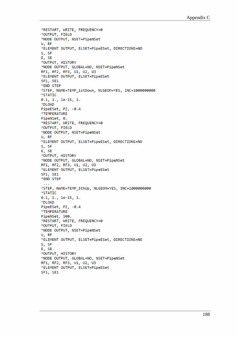
Appendix C
188

Appendix C
189

Appendix D
190
APPENDIX D
Appendix D provides the calculation check for lateral buckling for all models used in this
thesis (Chapters 3, 4, 5, 6 and 7). Although the coupled problem of walking and lateral
buckling is not the aim of this thesis, these calculations are provided here in order to show
that some cases studied are not susceptible to lateral buckling; whilst some other cases
are. Therefore, it can be understood that even illustration cases (i.e. cases that could suffer
lateral buckling) of the different soil characterization still have value for practical and
real situations. All cases (with or without lateral buckling susceptibility) follow through
the patterns established by this study.
Table D.1: Lateral buckling check
Chapter Model
Property Values
Buckle? L (m) W
(kN/m)
μ β (°) δmob /OD
3 1 3000 0.4 0.5 1 0.03 No
3 2 3000 0.4 0.5 1 0.05 No
3 3 3000 0.4 0.5 1 0.06 No
3 4 3000 0.4 0.5 1 0.1 No
3 5 3000 0.4 0.5 1 0.15 No
3 6 3000 0.4 0.5 1 0.2 No
3 7 3000 0.4 0.5 1 0.33 No
3 8 3000 0.4 0.5 1 0.5 No
3 9 3000 0.6 0.5 1 0.03 No
3 10 3000 0.6 0.5 1 0.05 No
3 11 3000 0.6 0.5 1 0.06 No
3 12 3000 0.6 0.5 1 0.1 No
3 13 3000 0.6 0.5 1 0.15 No
3 14 3000 0.6 0.5 1 0.2 No
3 15 3000 0.6 0.5 1 0.33 No
3 16 3000 0.6 0.5 1 0.5 No
3 17 3000 0.8 0.5 1 0.03 No
3 18 3000 0.8 0.5 1 0.05 No
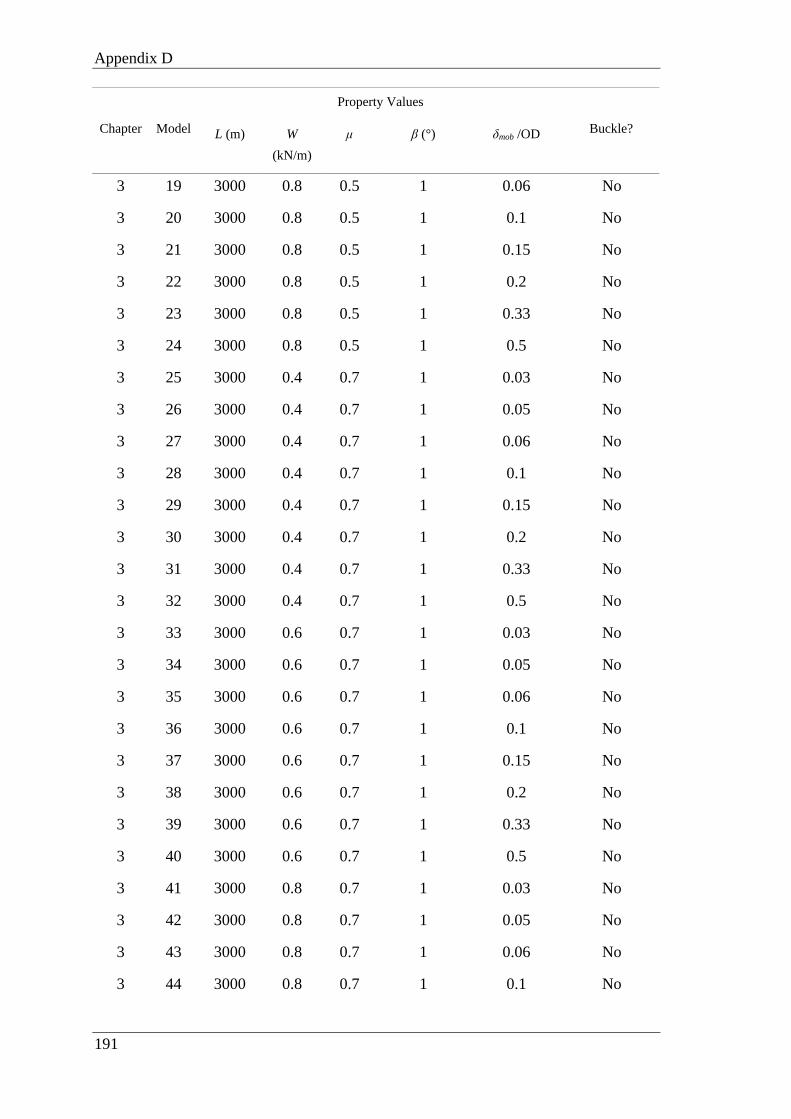
Appendix D
191
Chapter Model
Property Values
Buckle? L (m) W
(kN/m)
μ β (°) δmob /OD
3 19 3000 0.8 0.5 1 0.06 No
3 20 3000 0.8 0.5 1 0.1 No
3 21 3000 0.8 0.5 1 0.15 No
3 22 3000 0.8 0.5 1 0.2 No
3 23 3000 0.8 0.5 1 0.33 No
3 24 3000 0.8 0.5 1 0.5 No
3 25 3000 0.4 0.7 1 0.03 No
3 26 3000 0.4 0.7 1 0.05 No
3 27 3000 0.4 0.7 1 0.06 No
3 28 3000 0.4 0.7 1 0.1 No
3 29 3000 0.4 0.7 1 0.15 No
3 30 3000 0.4 0.7 1 0.2 No
3 31 3000 0.4 0.7 1 0.33 No
3 32 3000 0.4 0.7 1 0.5 No
3 33 3000 0.6 0.7 1 0.03 No
3 34 3000 0.6 0.7 1 0.05 No
3 35 3000 0.6 0.7 1 0.06 No
3 36 3000 0.6 0.7 1 0.1 No
3 37 3000 0.6 0.7 1 0.15 No
3 38 3000 0.6 0.7 1 0.2 No
3 39 3000 0.6 0.7 1 0.33 No
3 40 3000 0.6 0.7 1 0.5 No
3 41 3000 0.8 0.7 1 0.03 No
3 42 3000 0.8 0.7 1 0.05 No
3 43 3000 0.8 0.7 1 0.06 No
3 44 3000 0.8 0.7 1 0.1 No

Appendix D
192
Chapter Model
Property Values
Buckle? L (m) W
(kN/m)
μ β (°) δmob /OD
3 45 3000 0.8 0.7 1 0.15 No
3 46 3000 0.8 0.7 1 0.2 No
3 47 3000 0.8 0.7 1 0.33 No
3 48 3000 0.8 0.7 1 0.5 No
3 49 3000 0.4 0.9 1 0.03 Yes
3 50 3000 0.4 0.9 1 0.05 Yes
3 51 3000 0.4 0.9 1 0.06 Yes
3 52 3000 0.4 0.9 1 0.1 Yes
3 53 3000 0.4 0.9 1 0.15 Yes
3 54 3000 0.4 0.9 1 0.2 Yes
3 55 3000 0.4 0.9 1 0.33 Yes
3 56 3000 0.4 0.9 1 0.5 Yes
3 57 3000 0.6 0.9 1 0.03 Yes
3 58 3000 0.6 0.9 1 0.05 Yes
3 59 3000 0.6 0.9 1 0.06 Yes
3 60 3000 0.6 0.9 1 0.1 Yes
3 61 3000 0.6 0.9 1 0.15 Yes
3 62 3000 0.6 0.9 1 0.2 Yes
3 63 3000 0.6 0.9 1 0.33 Yes
3 64 3000 0.6 0.9 1 0.5 Yes
3 65 3000 0.8 0.9 1 0.03 Yes
3 66 3000 0.8 0.9 1 0.05 Yes
3 67 3000 0.8 0.9 1 0.06 Yes
3 68 3000 0.8 0.9 1 0.1 Yes
3 69 3000 0.8 0.9 1 0.15 Yes
3 70 3000 0.8 0.9 1 0.2 Yes
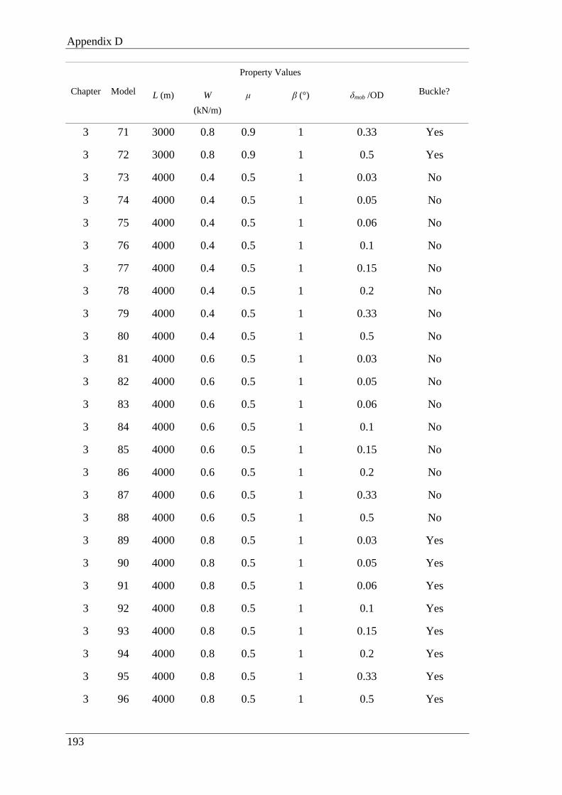
Appendix D
193
Chapter Model
Property Values
Buckle? L (m) W
(kN/m)
μ β (°) δmob /OD
3 71 3000 0.8 0.9 1 0.33 Yes
3 72 3000 0.8 0.9 1 0.5 Yes
3 73 4000 0.4 0.5 1 0.03 No
3 74 4000 0.4 0.5 1 0.05 No
3 75 4000 0.4 0.5 1 0.06 No
3 76 4000 0.4 0.5 1 0.1 No
3 77 4000 0.4 0.5 1 0.15 No
3 78 4000 0.4 0.5 1 0.2 No
3 79 4000 0.4 0.5 1 0.33 No
3 80 4000 0.4 0.5 1 0.5 No
3 81 4000 0.6 0.5 1 0.03 No
3 82 4000 0.6 0.5 1 0.05 No
3 83 4000 0.6 0.5 1 0.06 No
3 84 4000 0.6 0.5 1 0.1 No
3 85 4000 0.6 0.5 1 0.15 No
3 86 4000 0.6 0.5 1 0.2 No
3 87 4000 0.6 0.5 1 0.33 No
3 88 4000 0.6 0.5 1 0.5 No
3 89 4000 0.8 0.5 1 0.03 Yes
3 90 4000 0.8 0.5 1 0.05 Yes
3 91 4000 0.8 0.5 1 0.06 Yes
3 92 4000 0.8 0.5 1 0.1 Yes
3 93 4000 0.8 0.5 1 0.15 Yes
3 94 4000 0.8 0.5 1 0.2 Yes
3 95 4000 0.8 0.5 1 0.33 Yes
3 96 4000 0.8 0.5 1 0.5 Yes

Appendix D
194
Chapter Model
Property Values
Buckle? L (m) W
(kN/m)
μ β (°) δmob /OD
3 97 4000 0.4 0.7 1 0.03 No
3 98 4000 0.4 0.7 1 0.05 No
3 99 4000 0.4 0.7 1 0.06 No
3 100 4000 0.4 0.7 1 0.1 No
3 101 4000 0.4 0.7 1 0.15 No
3 102 4000 0.4 0.7 1 0.2 No
3 103 4000 0.4 0.7 1 0.33 No
3 104 4000 0.4 0.7 1 0.5 No
3 105 4000 0.6 0.7 1 0.03 Yes
3 106 4000 0.6 0.7 1 0.05 Yes
3 107 4000 0.6 0.7 1 0.06 Yes
3 108 4000 0.6 0.7 1 0.1 Yes
3 109 4000 0.6 0.7 1 0.15 Yes
3 110 4000 0.6 0.7 1 0.2 Yes
3 111 4000 0.6 0.7 1 0.33 Yes
3 112 4000 0.6 0.7 1 0.5 Yes
3 113 4000 0.8 0.7 1 0.03 Yes
3 114 4000 0.8 0.7 1 0.05 Yes
3 115 4000 0.8 0.7 1 0.06 Yes
3 116 4000 0.8 0.7 1 0.1 Yes
3 117 4000 0.8 0.7 1 0.15 Yes
3 118 4000 0.8 0.7 1 0.2 Yes
3 119 4000 0.8 0.7 1 0.33 Yes
3 120 4000 0.8 0.7 1 0.5 Yes
3 121 4000 0.4 0.9 1 0.03 Yes
3 122 4000 0.4 0.9 1 0.05 Yes

Appendix D
195
Chapter Model
Property Values
Buckle? L (m) W
(kN/m)
μ β (°) δmob /OD
3 123 4000 0.4 0.9 1 0.06 Yes
3 124 4000 0.4 0.9 1 0.1 Yes
3 125 4000 0.4 0.9 1 0.15 Yes
3 126 4000 0.4 0.9 1 0.2 Yes
3 127 4000 0.4 0.9 1 0.33 Yes
3 128 4000 0.4 0.9 1 0.5 Yes
3 129 4000 0.6 0.9 1 0.03 Yes
3 130 4000 0.6 0.9 1 0.05 Yes
3 131 4000 0.6 0.9 1 0.06 Yes
3 132 4000 0.6 0.9 1 0.1 Yes
3 133 4000 0.6 0.9 1 0.15 Yes
3 134 4000 0.6 0.9 1 0.2 Yes
3 135 4000 0.6 0.9 1 0.33 Yes
3 136 4000 0.6 0.9 1 0.5 Yes
3 137 4000 0.8 0.9 1 0.03 Yes
3 138 4000 0.8 0.9 1 0.05 Yes
3 139 4000 0.8 0.9 1 0.06 Yes
3 140 4000 0.8 0.9 1 0.1 Yes
3 141 4000 0.8 0.9 1 0.15 Yes
3 142 4000 0.8 0.9 1 0.2 Yes
3 143 4000 0.8 0.9 1 0.33 Yes
3 144 4000 0.8 0.9 1 0.5 Yes
3 145 5000 0.4 0.5 1 0.03 Yes
3 146 5000 0.4 0.5 1 0.05 Yes
3 147 5000 0.4 0.5 1 0.06 Yes
3 148 5000 0.4 0.5 1 0.1 Yes

Appendix D
196
Chapter Model
Property Values
Buckle? L (m) W
(kN/m)
μ β (°) δmob /OD
3 149 5000 0.4 0.5 1 0.15 Yes
3 150 5000 0.4 0.5 1 0.2 Yes
3 151 5000 0.4 0.5 1 0.33 Yes
3 152 5000 0.4 0.5 1 0.5 Yes
3 153 5000 0.6 0.5 1 0.03 Yes
3 154 5000 0.6 0.5 1 0.05 Yes
3 155 5000 0.6 0.5 1 0.06 Yes
3 156 5000 0.6 0.5 1 0.1 Yes
3 157 5000 0.6 0.5 1 0.15 Yes
3 158 5000 0.6 0.5 1 0.2 Yes
3 159 5000 0.6 0.5 1 0.33 Yes
3 160 5000 0.6 0.5 1 0.5 Yes
3 161 5000 0.8 0.5 1 0.03 Yes
3 162 5000 0.8 0.5 1 0.05 Yes
3 163 5000 0.8 0.5 1 0.06 Yes
3 164 5000 0.8 0.5 1 0.1 Yes
3 165 5000 0.8 0.5 1 0.15 Yes
3 166 5000 0.8 0.5 1 0.2 Yes
3 167 5000 0.8 0.5 1 0.33 Yes
3 168 5000 0.8 0.5 1 0.5 Yes
3 169 5000 0.4 0.7 1 0.03 Yes
3 170 5000 0.4 0.7 1 0.05 Yes
3 171 5000 0.4 0.7 1 0.06 Yes
3 172 5000 0.4 0.7 1 0.1 Yes
3 173 5000 0.4 0.7 1 0.15 Yes
3 174 5000 0.4 0.7 1 0.2 Yes

Appendix D
197
Chapter Model
Property Values
Buckle? L (m) W
(kN/m)
μ β (°) δmob /OD
3 175 5000 0.4 0.7 1 0.33 Yes
3 176 5000 0.4 0.7 1 0.5 Yes
3 177 5000 0.6 0.7 1 0.03 Yes
3 178 5000 0.6 0.7 1 0.05 Yes
3 179 5000 0.6 0.7 1 0.06 Yes
3 180 5000 0.6 0.7 1 0.1 Yes
3 181 5000 0.6 0.7 1 0.15 Yes
3 182 5000 0.6 0.7 1 0.2 Yes
3 183 5000 0.6 0.7 1 0.33 Yes
3 184 5000 0.6 0.7 1 0.5 Yes
3 185 5000 0.8 0.7 1 0.03 Yes
3 186 5000 0.8 0.7 1 0.05 Yes
3 187 5000 0.8 0.7 1 0.06 Yes
3 188 5000 0.8 0.7 1 0.1 Yes
3 189 5000 0.8 0.7 1 0.15 Yes
3 190 5000 0.8 0.7 1 0.2 Yes
3 191 5000 0.8 0.7 1 0.33 Yes
3 192 5000 0.8 0.7 1 0.5 Yes
3 193 5000 0.4 0.9 1 0.03 Yes
3 194 5000 0.4 0.9 1 0.05 Yes
3 195 5000 0.4 0.9 1 0.06 Yes
3 196 5000 0.4 0.9 1 0.1 Yes
3 197 5000 0.4 0.9 1 0.15 Yes
3 198 5000 0.4 0.9 1 0.2 Yes
3 199 5000 0.4 0.9 1 0.33 Yes
3 200 5000 0.4 0.9 1 0.5 Yes
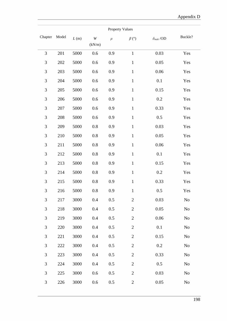
Appendix D
198
Chapter Model
Property Values
Buckle? L (m) W
(kN/m)
μ β (°) δmob /OD
3 201 5000 0.6 0.9 1 0.03 Yes
3 202 5000 0.6 0.9 1 0.05 Yes
3 203 5000 0.6 0.9 1 0.06 Yes
3 204 5000 0.6 0.9 1 0.1 Yes
3 205 5000 0.6 0.9 1 0.15 Yes
3 206 5000 0.6 0.9 1 0.2 Yes
3 207 5000 0.6 0.9 1 0.33 Yes
3 208 5000 0.6 0.9 1 0.5 Yes
3 209 5000 0.8 0.9 1 0.03 Yes
3 210 5000 0.8 0.9 1 0.05 Yes
3 211 5000 0.8 0.9 1 0.06 Yes
3 212 5000 0.8 0.9 1 0.1 Yes
3 213 5000 0.8 0.9 1 0.15 Yes
3 214 5000 0.8 0.9 1 0.2 Yes
3 215 5000 0.8 0.9 1 0.33 Yes
3 216 5000 0.8 0.9 1 0.5 Yes
3 217 3000 0.4 0.5 2 0.03 No
3 218 3000 0.4 0.5 2 0.05 No
3 219 3000 0.4 0.5 2 0.06 No
3 220 3000 0.4 0.5 2 0.1 No
3 221 3000 0.4 0.5 2 0.15 No
3 222 3000 0.4 0.5 2 0.2 No
3 223 3000 0.4 0.5 2 0.33 No
3 224 3000 0.4 0.5 2 0.5 No
3 225 3000 0.6 0.5 2 0.03 No
3 226 3000 0.6 0.5 2 0.05 No
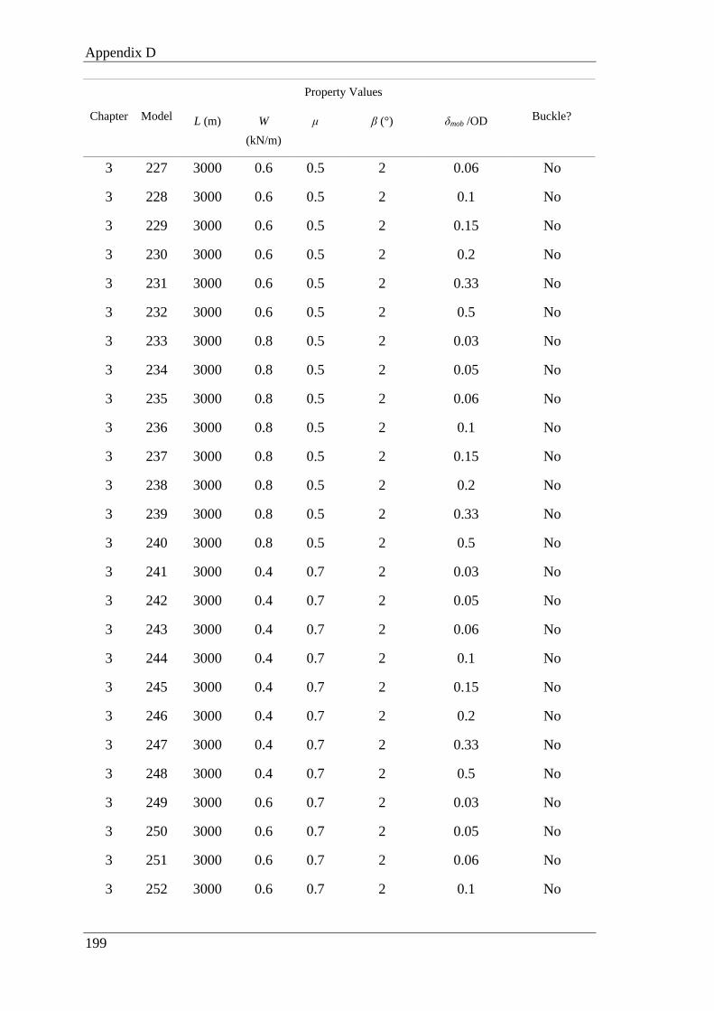
Appendix D
199
Chapter Model
Property Values
Buckle? L (m) W
(kN/m)
μ β (°) δmob /OD
3 227 3000 0.6 0.5 2 0.06 No
3 228 3000 0.6 0.5 2 0.1 No
3 229 3000 0.6 0.5 2 0.15 No
3 230 3000 0.6 0.5 2 0.2 No
3 231 3000 0.6 0.5 2 0.33 No
3 232 3000 0.6 0.5 2 0.5 No
3 233 3000 0.8 0.5 2 0.03 No
3 234 3000 0.8 0.5 2 0.05 No
3 235 3000 0.8 0.5 2 0.06 No
3 236 3000 0.8 0.5 2 0.1 No
3 237 3000 0.8 0.5 2 0.15 No
3 238 3000 0.8 0.5 2 0.2 No
3 239 3000 0.8 0.5 2 0.33 No
3 240 3000 0.8 0.5 2 0.5 No
3 241 3000 0.4 0.7 2 0.03 No
3 242 3000 0.4 0.7 2 0.05 No
3 243 3000 0.4 0.7 2 0.06 No
3 244 3000 0.4 0.7 2 0.1 No
3 245 3000 0.4 0.7 2 0.15 No
3 246 3000 0.4 0.7 2 0.2 No
3 247 3000 0.4 0.7 2 0.33 No
3 248 3000 0.4 0.7 2 0.5 No
3 249 3000 0.6 0.7 2 0.03 No
3 250 3000 0.6 0.7 2 0.05 No
3 251 3000 0.6 0.7 2 0.06 No
3 252 3000 0.6 0.7 2 0.1 No
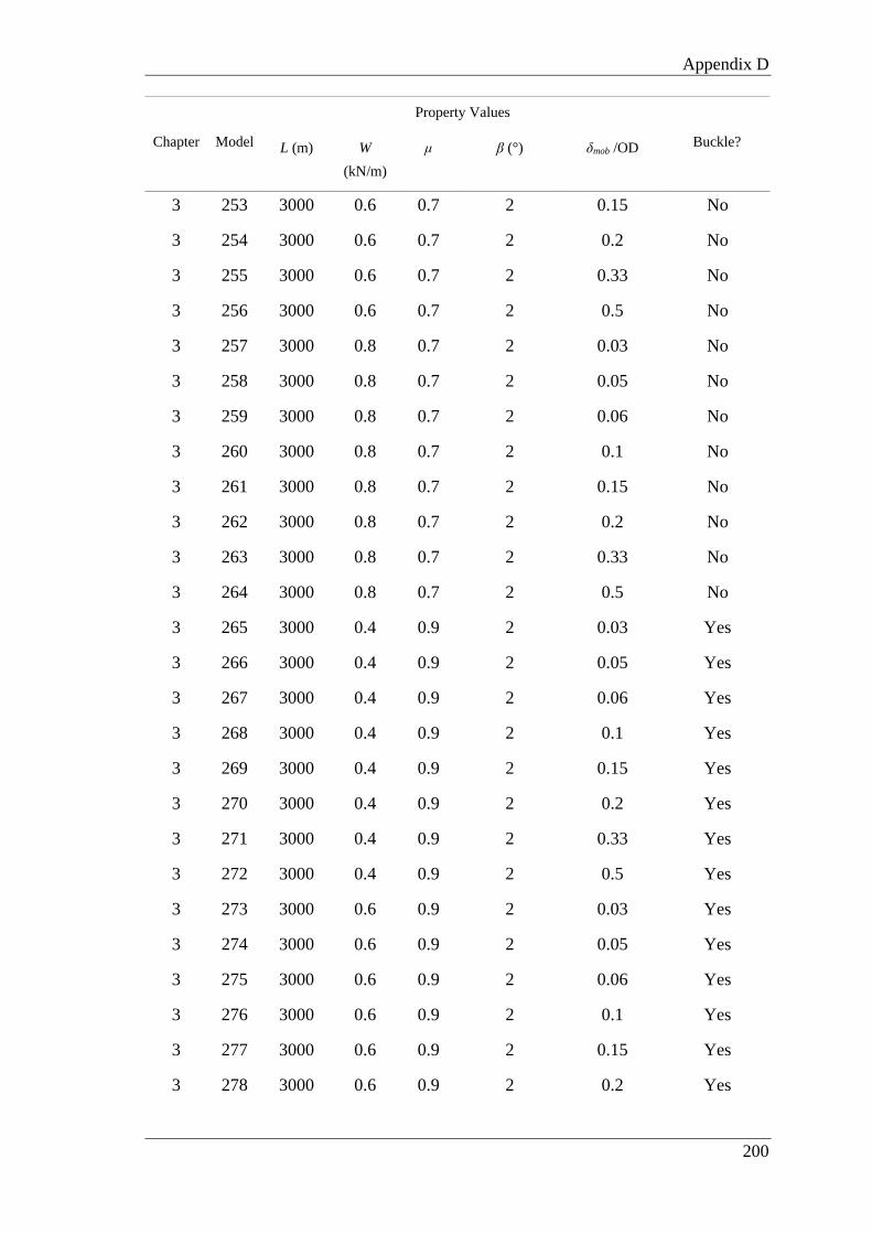
Appendix D
200
Chapter Model
Property Values
Buckle? L (m) W
(kN/m)
μ β (°) δmob /OD
3 253 3000 0.6 0.7 2 0.15 No
3 254 3000 0.6 0.7 2 0.2 No
3 255 3000 0.6 0.7 2 0.33 No
3 256 3000 0.6 0.7 2 0.5 No
3 257 3000 0.8 0.7 2 0.03 No
3 258 3000 0.8 0.7 2 0.05 No
3 259 3000 0.8 0.7 2 0.06 No
3 260 3000 0.8 0.7 2 0.1 No
3 261 3000 0.8 0.7 2 0.15 No
3 262 3000 0.8 0.7 2 0.2 No
3 263 3000 0.8 0.7 2 0.33 No
3 264 3000 0.8 0.7 2 0.5 No
3 265 3000 0.4 0.9 2 0.03 Yes
3 266 3000 0.4 0.9 2 0.05 Yes
3 267 3000 0.4 0.9 2 0.06 Yes
3 268 3000 0.4 0.9 2 0.1 Yes
3 269 3000 0.4 0.9 2 0.15 Yes
3 270 3000 0.4 0.9 2 0.2 Yes
3 271 3000 0.4 0.9 2 0.33 Yes
3 272 3000 0.4 0.9 2 0.5 Yes
3 273 3000 0.6 0.9 2 0.03 Yes
3 274 3000 0.6 0.9 2 0.05 Yes
3 275 3000 0.6 0.9 2 0.06 Yes
3 276 3000 0.6 0.9 2 0.1 Yes
3 277 3000 0.6 0.9 2 0.15 Yes
3 278 3000 0.6 0.9 2 0.2 Yes

Appendix D
201
Chapter Model
Property Values
Buckle? L (m) W
(kN/m)
μ β (°) δmob /OD
3 279 3000 0.6 0.9 2 0.33 Yes
3 280 3000 0.6 0.9 2 0.5 Yes
3 281 3000 0.8 0.9 2 0.03 Yes
3 282 3000 0.8 0.9 2 0.05 Yes
3 283 3000 0.8 0.9 2 0.06 Yes
3 284 3000 0.8 0.9 2 0.1 Yes
3 285 3000 0.8 0.9 2 0.15 Yes
3 286 3000 0.8 0.9 2 0.2 Yes
3 287 3000 0.8 0.9 2 0.33 Yes
3 288 3000 0.8 0.9 2 0.5 Yes
3 289 4000 0.4 0.5 2 0.03 No
3 290 4000 0.4 0.5 2 0.05 No
3 291 4000 0.4 0.5 2 0.06 No
3 292 4000 0.4 0.5 2 0.1 No
3 293 4000 0.4 0.5 2 0.15 No
3 294 4000 0.4 0.5 2 0.2 No
3 295 4000 0.4 0.5 2 0.33 No
3 296 4000 0.4 0.5 2 0.5 No
3 297 4000 0.6 0.5 2 0.03 No
3 298 4000 0.6 0.5 2 0.05 No
3 299 4000 0.6 0.5 2 0.06 No
3 300 4000 0.6 0.5 2 0.1 No
3 301 4000 0.6 0.5 2 0.15 No
3 302 4000 0.6 0.5 2 0.2 No
3 303 4000 0.6 0.5 2 0.33 No
3 304 4000 0.6 0.5 2 0.5 No

Appendix D
202
Chapter Model
Property Values
Buckle? L (m) W
(kN/m)
μ β (°) δmob /OD
3 305 4000 0.8 0.5 2 0.03 Yes
3 306 4000 0.8 0.5 2 0.05 Yes
3 307 4000 0.8 0.5 2 0.06 Yes
3 308 4000 0.8 0.5 2 0.1 Yes
3 309 4000 0.8 0.5 2 0.15 Yes
3 310 4000 0.8 0.5 2 0.2 Yes
3 311 4000 0.8 0.5 2 0.33 Yes
3 312 4000 0.8 0.5 2 0.5 Yes
3 313 4000 0.4 0.7 2 0.03 No
3 314 4000 0.4 0.7 2 0.05 No
3 315 4000 0.4 0.7 2 0.06 No
3 316 4000 0.4 0.7 2 0.1 No
3 317 4000 0.4 0.7 2 0.15 No
3 318 4000 0.4 0.7 2 0.2 No
3 319 4000 0.4 0.7 2 0.33 No
3 320 4000 0.4 0.7 2 0.5 No
3 321 4000 0.6 0.7 2 0.03 Yes
3 322 4000 0.6 0.7 2 0.05 Yes
3 323 4000 0.6 0.7 2 0.06 Yes
3 324 4000 0.6 0.7 2 0.1 Yes
3 325 4000 0.6 0.7 2 0.15 Yes
3 326 4000 0.6 0.7 2 0.2 Yes
3 327 4000 0.6 0.7 2 0.33 Yes
3 328 4000 0.6 0.7 2 0.5 Yes
3 329 4000 0.8 0.7 2 0.03 Yes
3 330 4000 0.8 0.7 2 0.05 Yes
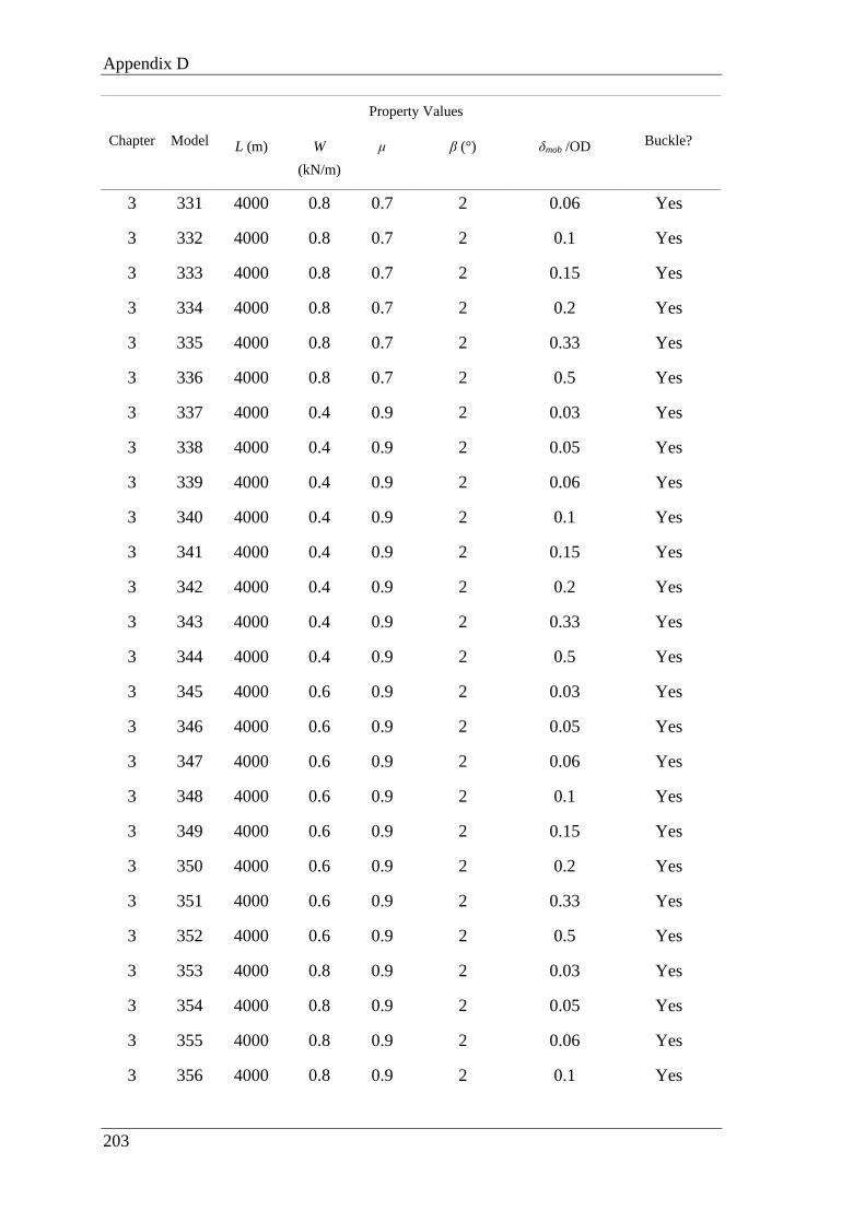
Appendix D
203
Chapter Model
Property Values
Buckle? L (m) W
(kN/m)
μ β (°) δmob /OD
3 331 4000 0.8 0.7 2 0.06 Yes
3 332 4000 0.8 0.7 2 0.1 Yes
3 333 4000 0.8 0.7 2 0.15 Yes
3 334 4000 0.8 0.7 2 0.2 Yes
3 335 4000 0.8 0.7 2 0.33 Yes
3 336 4000 0.8 0.7 2 0.5 Yes
3 337 4000 0.4 0.9 2 0.03 Yes
3 338 4000 0.4 0.9 2 0.05 Yes
3 339 4000 0.4 0.9 2 0.06 Yes
3 340 4000 0.4 0.9 2 0.1 Yes
3 341 4000 0.4 0.9 2 0.15 Yes
3 342 4000 0.4 0.9 2 0.2 Yes
3 343 4000 0.4 0.9 2 0.33 Yes
3 344 4000 0.4 0.9 2 0.5 Yes
3 345 4000 0.6 0.9 2 0.03 Yes
3 346 4000 0.6 0.9 2 0.05 Yes
3 347 4000 0.6 0.9 2 0.06 Yes
3 348 4000 0.6 0.9 2 0.1 Yes
3 349 4000 0.6 0.9 2 0.15 Yes
3 350 4000 0.6 0.9 2 0.2 Yes
3 351 4000 0.6 0.9 2 0.33 Yes
3 352 4000 0.6 0.9 2 0.5 Yes
3 353 4000 0.8 0.9 2 0.03 Yes
3 354 4000 0.8 0.9 2 0.05 Yes
3 355 4000 0.8 0.9 2 0.06 Yes
3 356 4000 0.8 0.9 2 0.1 Yes

Appendix D
204
Chapter Model
Property Values
Buckle? L (m) W
(kN/m)
μ β (°) δmob /OD
3 357 4000 0.8 0.9 2 0.15 Yes
3 358 4000 0.8 0.9 2 0.2 Yes
3 359 4000 0.8 0.9 2 0.33 Yes
3 360 4000 0.8 0.9 2 0.5 Yes
3 361 5000 0.4 0.5 2 0.03 Yes
3 362 5000 0.4 0.5 2 0.05 Yes
3 363 5000 0.4 0.5 2 0.06 Yes
3 364 5000 0.4 0.5 2 0.1 Yes
3 365 5000 0.4 0.5 2 0.15 Yes
3 366 5000 0.4 0.5 2 0.2 Yes
3 367 5000 0.4 0.5 2 0.33 Yes
3 368 5000 0.4 0.5 2 0.5 Yes
3 369 5000 0.6 0.5 2 0.03 Yes
3 370 5000 0.6 0.5 2 0.05 Yes
3 371 5000 0.6 0.5 2 0.06 Yes
3 372 5000 0.6 0.5 2 0.1 Yes
3 373 5000 0.6 0.5 2 0.15 Yes
3 374 5000 0.6 0.5 2 0.2 Yes
3 375 5000 0.6 0.5 2 0.33 Yes
3 376 5000 0.6 0.5 2 0.5 Yes
3 377 5000 0.8 0.5 2 0.03 Yes
3 378 5000 0.8 0.5 2 0.05 Yes
3 379 5000 0.8 0.5 2 0.06 Yes
3 380 5000 0.8 0.5 2 0.1 Yes
3 381 5000 0.8 0.5 2 0.15 Yes
3 382 5000 0.8 0.5 2 0.2 Yes
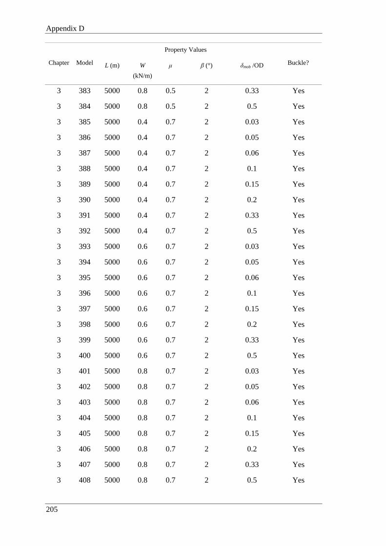
Appendix D
205
Chapter Model
Property Values
Buckle? L (m) W
(kN/m)
μ β (°) δmob /OD
3 383 5000 0.8 0.5 2 0.33 Yes
3 384 5000 0.8 0.5 2 0.5 Yes
3 385 5000 0.4 0.7 2 0.03 Yes
3 386 5000 0.4 0.7 2 0.05 Yes
3 387 5000 0.4 0.7 2 0.06 Yes
3 388 5000 0.4 0.7 2 0.1 Yes
3 389 5000 0.4 0.7 2 0.15 Yes
3 390 5000 0.4 0.7 2 0.2 Yes
3 391 5000 0.4 0.7 2 0.33 Yes
3 392 5000 0.4 0.7 2 0.5 Yes
3 393 5000 0.6 0.7 2 0.03 Yes
3 394 5000 0.6 0.7 2 0.05 Yes
3 395 5000 0.6 0.7 2 0.06 Yes
3 396 5000 0.6 0.7 2 0.1 Yes
3 397 5000 0.6 0.7 2 0.15 Yes
3 398 5000 0.6 0.7 2 0.2 Yes
3 399 5000 0.6 0.7 2 0.33 Yes
3 400 5000 0.6 0.7 2 0.5 Yes
3 401 5000 0.8 0.7 2 0.03 Yes
3 402 5000 0.8 0.7 2 0.05 Yes
3 403 5000 0.8 0.7 2 0.06 Yes
3 404 5000 0.8 0.7 2 0.1 Yes
3 405 5000 0.8 0.7 2 0.15 Yes
3 406 5000 0.8 0.7 2 0.2 Yes
3 407 5000 0.8 0.7 2 0.33 Yes
3 408 5000 0.8 0.7 2 0.5 Yes

Appendix D
206
Chapter Model
Property Values
Buckle? L (m) W
(kN/m)
μ β (°) δmob /OD
3 409 5000 0.4 0.9 2 0.03 Yes
3 410 5000 0.4 0.9 2 0.05 Yes
3 411 5000 0.4 0.9 2 0.06 Yes
3 412 5000 0.4 0.9 2 0.1 Yes
3 413 5000 0.4 0.9 2 0.15 Yes
3 414 5000 0.4 0.9 2 0.2 Yes
3 415 5000 0.4 0.9 2 0.33 Yes
3 416 5000 0.4 0.9 2 0.5 Yes
3 417 5000 0.6 0.9 2 0.03 Yes
3 418 5000 0.6 0.9 2 0.05 Yes
3 419 5000 0.6 0.9 2 0.06 Yes
3 420 5000 0.6 0.9 2 0.1 Yes
3 421 5000 0.6 0.9 2 0.15 Yes
3 422 5000 0.6 0.9 2 0.2 Yes
3 423 5000 0.6 0.9 2 0.33 Yes
3 424 5000 0.6 0.9 2 0.5 Yes
3 425 5000 0.8 0.9 2 0.03 Yes
3 426 5000 0.8 0.9 2 0.05 Yes
3 427 5000 0.8 0.9 2 0.06 Yes
3 428 5000 0.8 0.9 2 0.1 Yes
3 429 5000 0.8 0.9 2 0.15 Yes
3 430 5000 0.8 0.9 2 0.2 Yes
3 431 5000 0.8 0.9 2 0.33 Yes
3 432 5000 0.8 0.9 2 0.5 Yes
3 433 3000 0.4 0.5 3 0.03 No
3 434 3000 0.4 0.5 3 0.05 No
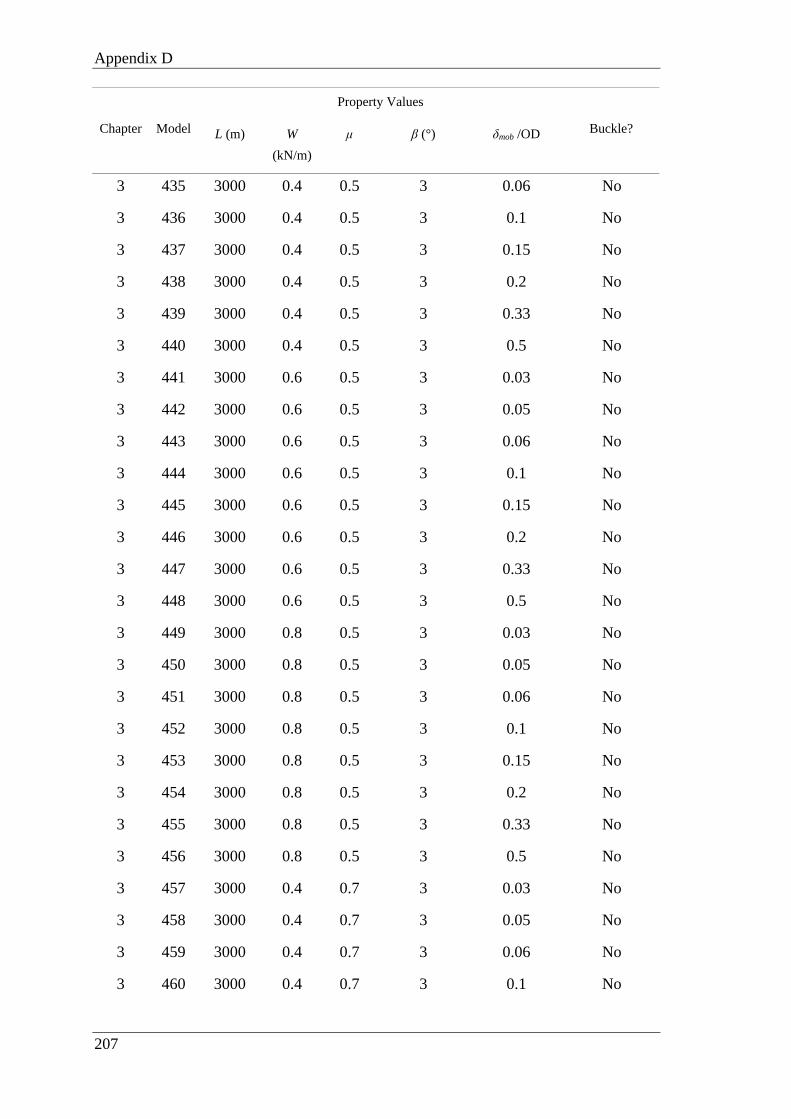
Appendix D
207
Chapter Model
Property Values
Buckle? L (m) W
(kN/m)
μ β (°) δmob /OD
3 435 3000 0.4 0.5 3 0.06 No
3 436 3000 0.4 0.5 3 0.1 No
3 437 3000 0.4 0.5 3 0.15 No
3 438 3000 0.4 0.5 3 0.2 No
3 439 3000 0.4 0.5 3 0.33 No
3 440 3000 0.4 0.5 3 0.5 No
3 441 3000 0.6 0.5 3 0.03 No
3 442 3000 0.6 0.5 3 0.05 No
3 443 3000 0.6 0.5 3 0.06 No
3 444 3000 0.6 0.5 3 0.1 No
3 445 3000 0.6 0.5 3 0.15 No
3 446 3000 0.6 0.5 3 0.2 No
3 447 3000 0.6 0.5 3 0.33 No
3 448 3000 0.6 0.5 3 0.5 No
3 449 3000 0.8 0.5 3 0.03 No
3 450 3000 0.8 0.5 3 0.05 No
3 451 3000 0.8 0.5 3 0.06 No
3 452 3000 0.8 0.5 3 0.1 No
3 453 3000 0.8 0.5 3 0.15 No
3 454 3000 0.8 0.5 3 0.2 No
3 455 3000 0.8 0.5 3 0.33 No
3 456 3000 0.8 0.5 3 0.5 No
3 457 3000 0.4 0.7 3 0.03 No
3 458 3000 0.4 0.7 3 0.05 No
3 459 3000 0.4 0.7 3 0.06 No
3 460 3000 0.4 0.7 3 0.1 No

Appendix D
208
Chapter Model
Property Values
Buckle? L (m) W
(kN/m)
μ β (°) δmob /OD
3 461 3000 0.4 0.7 3 0.15 No
3 462 3000 0.4 0.7 3 0.2 No
3 463 3000 0.4 0.7 3 0.33 No
3 464 3000 0.4 0.7 3 0.5 No
3 465 3000 0.6 0.7 3 0.03 No
3 466 3000 0.6 0.7 3 0.05 No
3 467 3000 0.6 0.7 3 0.06 No
3 468 3000 0.6 0.7 3 0.1 No
3 469 3000 0.6 0.7 3 0.15 No
3 470 3000 0.6 0.7 3 0.2 No
3 471 3000 0.6 0.7 3 0.33 No
3 472 3000 0.6 0.7 3 0.5 No
3 473 3000 0.8 0.7 3 0.03 No
3 474 3000 0.8 0.7 3 0.05 No
3 475 3000 0.8 0.7 3 0.06 No
3 476 3000 0.8 0.7 3 0.1 No
3 477 3000 0.8 0.7 3 0.15 No
3 478 3000 0.8 0.7 3 0.2 No
3 479 3000 0.8 0.7 3 0.33 No
3 480 3000 0.8 0.7 3 0.5 No
3 481 3000 0.4 0.9 3 0.03 Yes
3 482 3000 0.4 0.9 3 0.05 Yes
3 483 3000 0.4 0.9 3 0.06 Yes
3 484 3000 0.4 0.9 3 0.1 Yes
3 485 3000 0.4 0.9 3 0.15 Yes
3 486 3000 0.4 0.9 3 0.2 Yes

Appendix D
209
Chapter Model
Property Values
Buckle? L (m) W
(kN/m)
μ β (°) δmob /OD
3 487 3000 0.4 0.9 3 0.33 Yes
3 488 3000 0.4 0.9 3 0.5 Yes
3 489 3000 0.6 0.9 3 0.03 Yes
3 490 3000 0.6 0.9 3 0.05 Yes
3 491 3000 0.6 0.9 3 0.06 Yes
3 492 3000 0.6 0.9 3 0.1 Yes
3 493 3000 0.6 0.9 3 0.15 Yes
3 494 3000 0.6 0.9 3 0.2 Yes
3 495 3000 0.6 0.9 3 0.33 Yes
3 496 3000 0.6 0.9 3 0.5 Yes
3 497 3000 0.8 0.9 3 0.03 Yes
3 498 3000 0.8 0.9 3 0.05 Yes
3 499 3000 0.8 0.9 3 0.06 Yes
3 500 3000 0.8 0.9 3 0.1 Yes
3 501 3000 0.8 0.9 3 0.15 Yes
3 502 3000 0.8 0.9 3 0.2 Yes
3 503 3000 0.8 0.9 3 0.33 Yes
3 504 3000 0.8 0.9 3 0.5 Yes
3 505 4000 0.4 0.5 3 0.03 No
3 506 4000 0.4 0.5 3 0.05 No
3 507 4000 0.4 0.5 3 0.06 No
3 508 4000 0.4 0.5 3 0.1 No
3 509 4000 0.4 0.5 3 0.15 No
3 510 4000 0.4 0.5 3 0.2 No
3 511 4000 0.4 0.5 3 0.33 No
3 512 4000 0.4 0.5 3 0.5 No

Appendix D
210
Chapter Model
Property Values
Buckle? L (m) W
(kN/m)
μ β (°) δmob /OD
3 513 4000 0.6 0.5 3 0.03 No
3 514 4000 0.6 0.5 3 0.05 No
3 515 4000 0.6 0.5 3 0.06 No
3 516 4000 0.6 0.5 3 0.1 No
3 517 4000 0.6 0.5 3 0.15 No
3 518 4000 0.6 0.5 3 0.2 No
3 519 4000 0.6 0.5 3 0.33 No
3 520 4000 0.6 0.5 3 0.5 No
3 521 4000 0.8 0.5 3 0.03 Yes
3 522 4000 0.8 0.5 3 0.05 Yes
3 523 4000 0.8 0.5 3 0.06 Yes
3 524 4000 0.8 0.5 3 0.1 Yes
3 525 4000 0.8 0.5 3 0.15 Yes
3 526 4000 0.8 0.5 3 0.2 Yes
3 527 4000 0.8 0.5 3 0.33 Yes
3 528 4000 0.8 0.5 3 0.5 Yes
3 529 4000 0.4 0.7 3 0.03 No
3 530 4000 0.4 0.7 3 0.05 No
3 531 4000 0.4 0.7 3 0.06 No
3 532 4000 0.4 0.7 3 0.1 No
3 533 4000 0.4 0.7 3 0.15 No
3 534 4000 0.4 0.7 3 0.2 No
3 535 4000 0.4 0.7 3 0.33 No
3 536 4000 0.4 0.7 3 0.5 No
3 537 4000 0.6 0.7 3 0.03 Yes
3 538 4000 0.6 0.7 3 0.05 Yes

Appendix D
211
Chapter Model
Property Values
Buckle? L (m) W
(kN/m)
μ β (°) δmob /OD
3 539 4000 0.6 0.7 3 0.06 Yes
3 540 4000 0.6 0.7 3 0.1 Yes
3 541 4000 0.6 0.7 3 0.15 Yes
3 542 4000 0.6 0.7 3 0.2 Yes
3 543 4000 0.6 0.7 3 0.33 Yes
3 544 4000 0.6 0.7 3 0.5 Yes
3 545 4000 0.8 0.7 3 0.03 Yes
3 546 4000 0.8 0.7 3 0.05 Yes
3 547 4000 0.8 0.7 3 0.06 Yes
3 548 4000 0.8 0.7 3 0.1 Yes
3 549 4000 0.8 0.7 3 0.15 Yes
3 550 4000 0.8 0.7 3 0.2 Yes
3 551 4000 0.8 0.7 3 0.33 Yes
3 552 4000 0.8 0.7 3 0.5 Yes
3 553 4000 0.4 0.9 3 0.03 Yes
3 554 4000 0.4 0.9 3 0.05 Yes
3 555 4000 0.4 0.9 3 0.06 Yes
3 556 4000 0.4 0.9 3 0.1 Yes
3 557 4000 0.4 0.9 3 0.15 Yes
3 558 4000 0.4 0.9 3 0.2 Yes
3 559 4000 0.4 0.9 3 0.33 Yes
3 560 4000 0.4 0.9 3 0.5 Yes
3 561 4000 0.6 0.9 3 0.03 Yes
3 562 4000 0.6 0.9 3 0.05 Yes
3 563 4000 0.6 0.9 3 0.06 Yes
3 564 4000 0.6 0.9 3 0.1 Yes

Appendix D
212
Chapter Model
Property Values
Buckle? L (m) W
(kN/m)
μ β (°) δmob /OD
3 565 4000 0.6 0.9 3 0.15 Yes
3 566 4000 0.6 0.9 3 0.2 Yes
3 567 4000 0.6 0.9 3 0.33 Yes
3 568 4000 0.6 0.9 3 0.5 Yes
3 569 4000 0.8 0.9 3 0.03 Yes
3 570 4000 0.8 0.9 3 0.05 Yes
3 571 4000 0.8 0.9 3 0.06 Yes
3 572 4000 0.8 0.9 3 0.1 Yes
3 573 4000 0.8 0.9 3 0.15 Yes
3 574 4000 0.8 0.9 3 0.2 Yes
3 575 4000 0.8 0.9 3 0.33 Yes
3 576 4000 0.8 0.9 3 0.5 Yes
3 577 5000 0.4 0.5 3 0.03 Yes
3 578 5000 0.4 0.5 3 0.05 Yes
3 579 5000 0.4 0.5 3 0.06 Yes
3 580 5000 0.4 0.5 3 0.1 Yes
3 581 5000 0.4 0.5 3 0.15 Yes
3 582 5000 0.4 0.5 3 0.2 Yes
3 583 5000 0.4 0.5 3 0.33 Yes
3 584 5000 0.4 0.5 3 0.5 Yes
3 585 5000 0.6 0.5 3 0.03 Yes
3 586 5000 0.6 0.5 3 0.05 Yes
3 587 5000 0.6 0.5 3 0.06 Yes
3 588 5000 0.6 0.5 3 0.1 Yes
3 589 5000 0.6 0.5 3 0.15 Yes
3 590 5000 0.6 0.5 3 0.2 Yes

Appendix D
213
Chapter Model
Property Values
Buckle? L (m) W
(kN/m)
μ β (°) δmob /OD
3 591 5000 0.6 0.5 3 0.33 Yes
3 592 5000 0.6 0.5 3 0.5 Yes
3 593 5000 0.8 0.5 3 0.03 Yes
3 594 5000 0.8 0.5 3 0.05 Yes
3 595 5000 0.8 0.5 3 0.06 Yes
3 596 5000 0.8 0.5 3 0.1 Yes
3 597 5000 0.8 0.5 3 0.15 Yes
3 598 5000 0.8 0.5 3 0.2 Yes
3 599 5000 0.8 0.5 3 0.33 Yes
3 600 5000 0.8 0.5 3 0.5 Yes
3 601 5000 0.4 0.7 3 0.03 Yes
3 602 5000 0.4 0.7 3 0.05 Yes
3 603 5000 0.4 0.7 3 0.06 Yes
3 604 5000 0.4 0.7 3 0.1 Yes
3 605 5000 0.4 0.7 3 0.15 Yes
3 606 5000 0.4 0.7 3 0.2 Yes
3 607 5000 0.4 0.7 3 0.33 Yes
3 608 5000 0.4 0.7 3 0.5 Yes
3 609 5000 0.6 0.7 3 0.03 Yes
3 610 5000 0.6 0.7 3 0.05 Yes
3 611 5000 0.6 0.7 3 0.06 Yes
3 612 5000 0.6 0.7 3 0.1 Yes
3 613 5000 0.6 0.7 3 0.15 Yes
3 614 5000 0.6 0.7 3 0.2 Yes
3 615 5000 0.6 0.7 3 0.33 Yes
3 616 5000 0.6 0.7 3 0.5 Yes

Appendix D
214
Chapter Model
Property Values
Buckle? L (m) W
(kN/m)
μ β (°) δmob /OD
3 617 5000 0.8 0.7 3 0.03 Yes
3 618 5000 0.8 0.7 3 0.05 Yes
3 619 5000 0.8 0.7 3 0.06 Yes
3 620 5000 0.8 0.7 3 0.1 Yes
3 621 5000 0.8 0.7 3 0.15 Yes
3 622 5000 0.8 0.7 3 0.2 Yes
3 623 5000 0.8 0.7 3 0.33 Yes
3 624 5000 0.8 0.7 3 0.5 Yes
3 625 5000 0.4 0.9 3 0.03 Yes
3 626 5000 0.4 0.9 3 0.05 Yes
3 627 5000 0.4 0.9 3 0.06 Yes
3 628 5000 0.4 0.9 3 0.1 Yes
3 629 5000 0.4 0.9 3 0.15 Yes
3 630 5000 0.4 0.9 3 0.2 Yes
3 631 5000 0.4 0.9 3 0.33 Yes
3 632 5000 0.4 0.9 3 0.5 Yes
3 633 5000 0.6 0.9 3 0.03 Yes
3 634 5000 0.6 0.9 3 0.05 Yes
3 635 5000 0.6 0.9 3 0.06 Yes
3 636 5000 0.6 0.9 3 0.1 Yes
3 637 5000 0.6 0.9 3 0.15 Yes
3 638 5000 0.6 0.9 3 0.2 Yes
3 639 5000 0.6 0.9 3 0.33 Yes
3 640 5000 0.6 0.9 3 0.5 Yes
3 641 5000 0.8 0.9 3 0.03 Yes
3 642 5000 0.8 0.9 3 0.05 Yes

Appendix D
215
Chapter Model
Property Values
Buckle? L (m) W
(kN/m)
μ β (°) δmob /OD
3 643 5000 0.8 0.9 3 0.06 Yes
3 644 5000 0.8 0.9 3 0.1 Yes
3 645 5000 0.8 0.9 3 0.15 Yes
3 646 5000 0.8 0.9 3 0.2 Yes
3 647 5000 0.8 0.9 3 0.33 Yes
3 648 5000 0.8 0.9 3 0.5 Yes
4 1 5000 0.8 0.5 1 0.0825 Yes
4 2 5000 0.8 0.5 1 0.065 Yes
4 3 5000 0.8 0.5 1 0.0475 Yes
4 4 5000 0.8 0.5 1 0.0825 Yes
4 5 5000 0.8 0.5 1 0.0650 Yes
4 6 5000 0.8 0.5 1 0.0825 Yes
4 7 5000 0.8 0.5 1 0.1237 Yes
4 8 5000 0.8 0.5 1 0.0975 Yes
4 9 5000 0.8 0.5 1 0.0712 Yes
4 10 5000 0.8 0.5 1 0.1237 Yes
4 11 5000 0.8 0.5 1 0.0975 Yes
4 12 5000 0.8 0.5 1 0.1237 Yes
4 13 5000 0.8 0.5 1 0.165 Yes
4 14 5000 0.8 0.5 1 0.13 Yes
4 15 5000 0.8 0.5 1 0.095 Yes
4 16 5000 0.8 0.5 1 0.1650 Yes
4 17 5000 0.8 0.5 1 0.13 Yes
4 18 5000 0.8 0.5 1 0.165 Yes
4 19 5000 0.8 0.5 1 0.2747 Yes
4 20 5000 0.8 0.5 1 0.2164 Yes

Appendix D
216
Chapter Model
Property Values
Buckle? L (m) W
(kN/m)
μ β (°) δmob /OD
4 21 5000 0.8 0.5 1 0.15818 Yes
4 22 5000 0.8 0.5 1 0.2747 Yes
4 23 5000 0.8 0.5 1 0.2164 Yes
4 24 5000 0.8 0.5 1 0.2747 Yes
4 25 5000 0.8 0.5 1 0.4125 Yes
4 26 5000 0.8 0.5 1 0.325 Yes
4 27 5000 0.8 0.5 1 0.2375 Yes
4 28 5000 0.8 0.5 1 0.4125 Yes
4 29 5000 0.8 0.5 1 0.3250 Yes
4 30 5000 0.8 0.5 1 0.4125 Yes
4 31 5000 0.8 0.5 2 0.0825 Yes
4 32 5000 0.8 0.5 2 0.065 Yes
4 33 5000 0.8 0.5 2 0.0475 Yes
4 34 5000 0.8 0.5 2 0.0825 Yes
4 35 5000 0.8 0.5 2 0.065 Yes
4 36 5000 0.8 0.5 2 0.0825 Yes
4 37 5000 0.8 0.5 2 0.12375 Yes
4 38 5000 0.8 0.5 2 0.0975 Yes
4 39 5000 0.8 0.5 2 0.07125 Yes
4 40 5000 0.8 0.5 2 0.1237 Yes
4 41 5000 0.8 0.5 2 0.0975 Yes
4 42 5000 0.8 0.5 2 0.1237 Yes
4 43 5000 0.8 0.5 2 0.165 Yes
4 44 5000 0.8 0.5 2 0.13 Yes
4 45 5000 0.8 0.5 2 0.095 Yes
4 46 5000 0.8 0.5 2 0.165 Yes

Appendix D
217
Chapter Model
Property Values
Buckle? L (m) W
(kN/m)
μ β (°) δmob /OD
4 47 5000 0.8 0.5 2 0.13 Yes
4 48 5000 0.8 0.5 2 0.165 Yes
4 49 5000 0.8 0.5 2 0.2747 Yes
4 50 5000 0.8 0.5 2 0.2164 Yes
4 51 5000 0.8 0.5 2 0.1581 Yes
4 52 5000 0.8 0.5 2 0.2747 Yes
4 53 5000 0.8 0.5 2 0.2164 Yes
4 54 5000 0.8 0.5 2 0.2747 Yes
4 55 5000 0.8 0.5 2 0.4125 Yes
4 56 5000 0.8 0.5 2 0.325 Yes
4 57 5000 0.8 0.5 2 0.2375 Yes
4 58 5000 0.8 0.5 2 0.4125 Yes
4 59 5000 0.8 0.5 2 0.325 Yes
4 60 5000 0.8 0.5 2 0.4125 Yes
4 61 5000 0.8 0.5 3 0.0825 Yes
4 62 5000 0.8 0.5 3 0.065 Yes
4 63 5000 0.8 0.5 3 0.0475 Yes
4 64 5000 0.8 0.5 3 0.0825 Yes
4 65 5000 0.8 0.5 3 0.0645 Yes
4 66 5000 0.8 0.5 3 0.0825 Yes
4 67 5000 0.8 0.5 3 0.1237 Yes
4 68 5000 0.8 0.5 3 0.0975 Yes
4 69 5000 0.8 0.5 3 0.0712 Yes
4 70 5000 0.8 0.5 3 0.1237 Yes
4 71 5000 0.8 0.5 3 0.0975 Yes
4 72 5000 0.8 0.5 3 0.1237 Yes

Appendix D
218
Chapter Model
Property Values
Buckle? L (m) W
(kN/m)
μ β (°) δmob /OD
4 73 5000 0.8 0.5 3 0.165 Yes
4 74 5000 0.8 0.5 3 0.13 Yes
4 75 5000 0.8 0.5 3 0.095 Yes
4 76 5000 0.8 0.5 3 0.1650 Yes
4 77 5000 0.8 0.5 3 0.13 Yes
4 78 5000 0.8 0.5 3 0.165 Yes
4 79 5000 0.8 0.5 3 0.2747 Yes
4 80 5000 0.8 0.5 3 0.2164 Yes
4 81 5000 0.8 0.5 3 0.1582 Yes
4 82 5000 0.8 0.5 3 0.2747 Yes
4 83 5000 0.8 0.5 3 0.2164 Yes
4 84 5000 0.8 0.5 3 0.2747 Yes
4 85 5000 0.8 0.5 3 0.4125 Yes
4 86 5000 0.8 0.5 3 0.325 Yes
4 87 5000 0.8 0.5 3 0.2375 Yes
4 88 5000 0.8 0.5 3 0.4125 Yes
4 89 5000 0.8 0.5 3 0.325 Yes
4 90 5000 0.8 0.5 3 0.4125 Yes
4 91 5000 0.4 0.5 3 0.2068 Yes
5 1 5000 0.40 0.25 2 0.2 No
5 2 5000 0.40 0.25 2 0.2 No
5 3 5000 0.40 0.25 2 0.2 No
5 4 5000 0.40 0.25 2 0.1 No
5 5 5000 0.40 0.25 2 0.1 No
5 6 5000 0.40 0.25 2 0.1 No
5 7 5000 0.40 0.25 2 0.1333 No

Appendix D
219
Chapter Model
Property Values
Buckle? L (m) W
(kN/m)
μ β (°) δmob /OD
5 8 5000 0.40 0.25 2 0.1333 No
5 9 5000 0.40 0.25 2 0.1333 No
5 10 5000 0.40 0.25 2 0.16 No
5 11 5000 0.40 0.25 2 0.16 No
5 12 5000 0.40 0.25 2 0.16 No
6 1 5000 0.40 0.25 2 0.1 No
6 2 5000 0.40 0.25 2 0.0768 No
7 1 3000 0.8 0.5 2 0.1235 Yes
7 2 3000 0.8 0.7 2 0.1235 Yes
7 3 3000 0.8 0.9 2 0.1235 Yes
7 4 4000 0.8 0.5 2 0.1235 Yes
7 5 4000 0.8 0.7 2 0.1235 Yes
7 6 4000 0.8 0.9 2 0.1235 Yes
7 7 5000 0.8 0.5 2 0.1235 Yes
7 8 5000 0.8 0.7 2 0.1235 Yes
7 9 5000 0.8 0.9 2 0.1235 Yes
7 10 5000 0.8 0.9 3 0.1235 Yes
7 11 3000 0.8 0.9 3 0.1235 Yes
7 12 4000 0.8 0.9 3 0.1235 Yes
7 13 4000 0.8 0.7 3 0.1235 Yes
7 14 5000 0.8 0.9 5 0.1235 Yes
7 15 5000 0.8 0.9 4.6 0.1235 Yes
7 16 5000 0.8 0.9 3.8 0.1235 Yes
7 17 5000 0.8 0.9 2.6 0.1235 Yes
7 18 5000 0.8 0.9 2 0.1235 Yes
7 19 4000 0.8 0.9 5 0.1235 Yes

Appendix D
220
Chapter Model
Property Values
Buckle? L (m) W
(kN/m)
μ β (°) δmob /OD
7 20 4000 0.8 0.9 4.5 0.1235 Yes
7 21 4000 0.8 0.9 4 0.1235 Yes
7 22 4000 0.8 0.9 4.5 0.1235 Yes
7 23 3000 0.8 0.9 4.3333 0.1235 Yes
7 24 3000 0.8 0.9 4 0.1235 Yes
7 25 3000 0.8 0.9 5 0.1235 Yes
7 26 3000 0.8 0.9 4.3333 0.1235 Yes
7 27 3000 0.8 0.5 2 0.1235 Yes
7 28 3000 0.8 0.7 2 0.1235 Yes
7 29 3000 0.8 0.9 2 0.1235 Yes
7 30 4000 0.8 0.5 2 0.1235 Yes
7 31 4000 0.8 0.7 2 0.1235 Yes
7 32 4000 0.8 0.9 2 0.1235 Yes
7 33 5000 0.8 0.5 2 0.1235 Yes
7 34 5000 0.8 0.7 2 0.1235 Yes
7 35 5000 0.8 0.9 2 0.1235 Yes
7 36 5000 0.8 0.9 3 0.1235 Yes
7 37 3000 0.8 0.9 3 0.1235 Yes
7 38 4000 0.8 0.9 3 0.1235 Yes
7 39 4000 0.8 0.7 3 0.1235 Yes
7 40 5000 0.8 0.9 5 0.1235 Yes
7 41 5000 0.8 0.9 4.3 0.1235 Yes
7 42 5000 0.8 0.9 3.94 0.1235 Yes
7 43 5000 0.8 0.9 3.42 0.1235 Yes
7 44 5000 0.8 0.9 4.42 0.1235 Yes
7 45 4000 0.8 0.9 5 0.1235 Yes
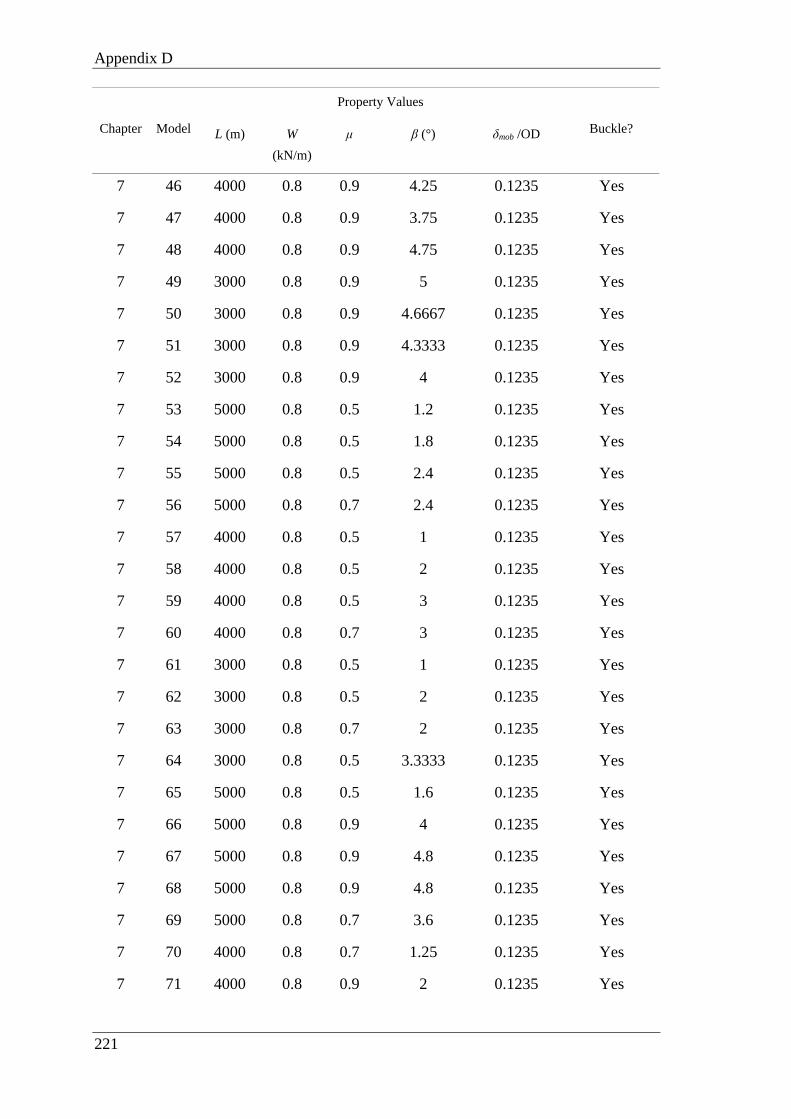
Appendix D
221
Chapter Model
Property Values
Buckle? L (m) W
(kN/m)
μ β (°) δmob /OD
7 46 4000 0.8 0.9 4.25 0.1235 Yes
7 47 4000 0.8 0.9 3.75 0.1235 Yes
7 48 4000 0.8 0.9 4.75 0.1235 Yes
7 49 3000 0.8 0.9 5 0.1235 Yes
7 50 3000 0.8 0.9 4.6667 0.1235 Yes
7 51 3000 0.8 0.9 4.3333 0.1235 Yes
7 52 3000 0.8 0.9 4 0.1235 Yes
7 53 5000 0.8 0.5 1.2 0.1235 Yes
7 54 5000 0.8 0.5 1.8 0.1235 Yes
7 55 5000 0.8 0.5 2.4 0.1235 Yes
7 56 5000 0.8 0.7 2.4 0.1235 Yes
7 57 4000 0.8 0.5 1 0.1235 Yes
7 58 4000 0.8 0.5 2 0.1235 Yes
7 59 4000 0.8 0.5 3 0.1235 Yes
7 60 4000 0.8 0.7 3 0.1235 Yes
7 61 3000 0.8 0.5 1 0.1235 Yes
7 62 3000 0.8 0.5 2 0.1235 Yes
7 63 3000 0.8 0.7 2 0.1235 Yes
7 64 3000 0.8 0.5 3.3333 0.1235 Yes
7 65 5000 0.8 0.5 1.6 0.1235 Yes
7 66 5000 0.8 0.9 4 0.1235 Yes
7 67 5000 0.8 0.9 4.8 0.1235 Yes
7 68 5000 0.8 0.9 4.8 0.1235 Yes
7 69 5000 0.8 0.7 3.6 0.1235 Yes
7 70 4000 0.8 0.7 1.25 0.1235 Yes
7 71 4000 0.8 0.9 2 0.1235 Yes

Appendix D
222
Chapter Model
Property Values
Buckle? L (m) W
(kN/m)
μ β (°) δmob /OD
7 72 4000 0.8 0.9 3 0.1235 Yes
7 73 4000 0.8 0.9 2.5 0.1235 Yes
7 74 3000 0.8 0.5 2 0.1235 Yes
7 75 3000 0.8 0.7 2 0.1235 Yes
7 76 3000 0.8 0.7 1.3333 0.1235 Yes
7 77 3000 0.8 0.7 2 0.1235 Yes
7 78 3000 0.8 0.9 2 0.1235 Yes
7 79 5000 0.8 0.5 1.8 0.1235 Yes
7 80 5000 0.8 0.5 1.2 0.1235 Yes
7 81 5000 0.8 0.5 0.6 0.1235 Yes
7 82 5000 0.8 0.7 0.6 0.1235 Yes
7 83 4000 0.8 0.7 3 0.1235 Yes
7 84 4000 0.8 0.7 2 0.1235 Yes
7 85 4000 0.8 0.5 1 0.1235 Yes
7 86 4000 0.8 0.7 1 0.1235 Yes
7 87 3000 0.8 0.5 2 0.1235 Yes
7 88 3000 0.8 0.5 1 0.1235 Yes
7 89 3000 0.8 0.7 1 0.1235 Yes
7 90 3000 0.8 0.7 1.6667 0.1235 Yes
7 91 5000 0.8 0.5 0.4 0.1235 Yes
7 92 5000 0.8 0.9 2 0.1235 Yes
7 93 5000 0.8 0.9 2.7 0.1235 Yes
7 94 5000 0.8 0.9 3.2 0.1235 Yes
7 95 5000 0.8 0.9 1.6 0.1235 Yes
7 96 4000 0.8 0.9 4.375 0.1235 Yes
7 97 4000 0.8 0.5 1.25 0.1235 Yes
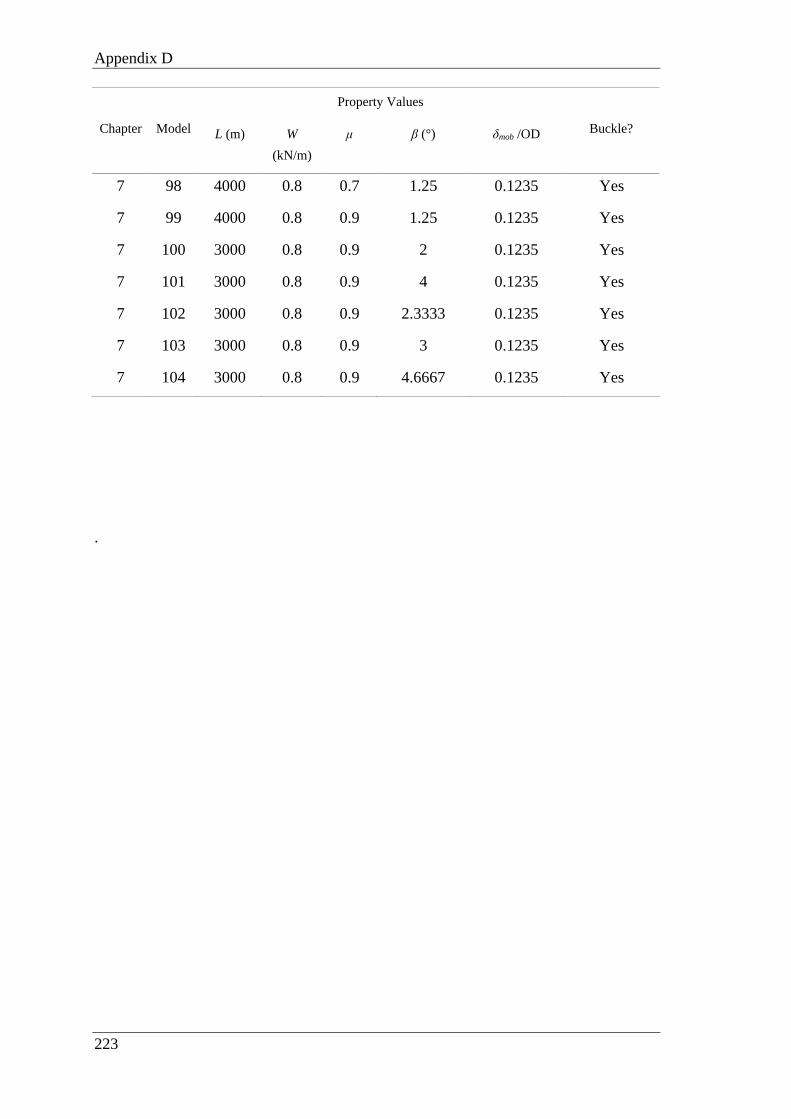
Appendix D
223
Chapter Model
Property Values
Buckle? L (m) W
(kN/m)
μ β (°) δmob /OD
7 98 4000 0.8 0.7 1.25 0.1235 Yes
7 99 4000 0.8 0.9 1.25 0.1235 Yes
7 100 3000 0.8 0.9 2 0.1235 Yes
7 101 3000 0.8 0.9 4 0.1235 Yes
7 102 3000 0.8 0.9 2.3333 0.1235 Yes
7 103 3000 0.8 0.9 3 0.1235 Yes
7 104 3000 0.8 0.9 4.6667 0.1235 Yes
.


![SUBSEA PIPELINE WALKING WITH VELOCITY DEPENDENT … · walking and lateral buckling. Even though a significant amount of experimental data on axial friction has been available [1],](https://img.pdfslide.net/doc/110x75/5ea34dea10d5527bb622ce2c/subsea-pipeline-walking-with-velocity-dependent-walking-and-lateral-buckling-even.jpg)