Dr. Jie Zou PHY3320 1

Chapter 8

Numerical IntegrationLecture (I)1

1 Ref.: “Applied Numerical Methods with MATLAB for Engineers and Scientists”, Steven Chapra, 2nd ed., Ch. 17, McGraw Hill, 2008.

Dr. Jie Zou PHY3320 2

Outline Introduction

What is integration? When do we need numerical integration?

Applications of integration in engineering and science

Newton-cotes formulas (1) The trapezoidal rule

Error of the Trapezoidal rule The composite trapezoidal rule Implementation in MATLAB

Dr. Jie Zou PHY3320 3

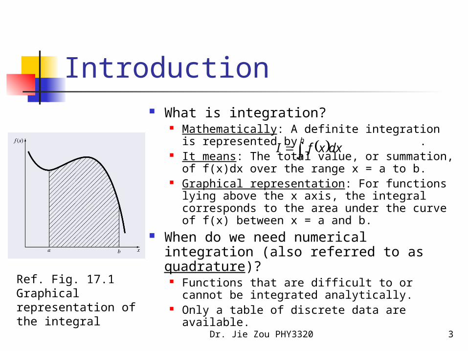
Introduction What is integration?

Mathematically: A definite integration is represented by .

It means: The total value, or summation, of f(x)dx over the range x = a to b.

Graphical representation: For functions lying above the x axis, the integral corresponds to the area under the curve of f(x) between x = a and b.

When do we need numerical integration (also referred to as quadrature)?

Functions that are difficult to or cannot be integrated analytically.

Only a table of discrete data are available.

b

adxxfI

Ref. Fig. 17.1 Graphical representation of the integral

Dr. Jie Zou PHY3320 4

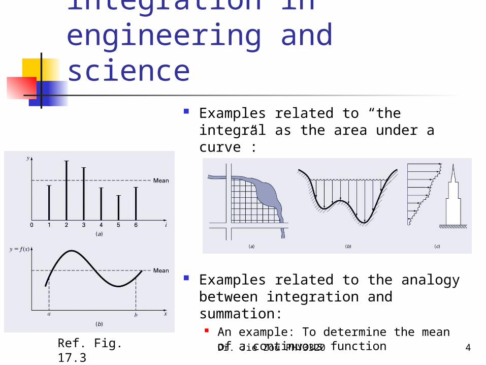
Applications of integration in engineering and science

Examples related to “the integral as the area under a curve”:

Examples related to the analogy between integration and summation:

An example: To determine the mean of a continuous functionRef. Fig. 17.3

Dr. Jie Zou PHY3320 5

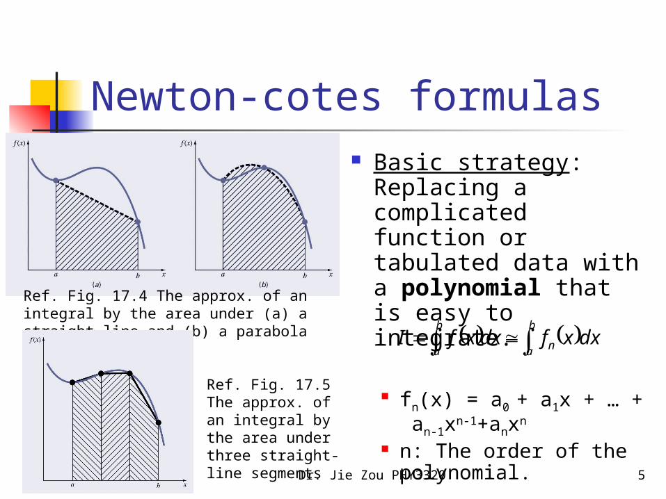
Newton-cotes formulas Basic strategy:

Replacing a complicated function or tabulated data with a polynomial that is easy to integrate.

fn(x) = a0 + a1x + … + an-1xn-1+anxn

n: The order of the polynomial.

b

a n

b

adxxfdxxfI

Ref. Fig. 17.4 The approx. of an integral by the area under (a) a straight line and (b) a parabola

Ref. Fig. 17.5 The approx. of an integral by the area under three straight-line segments

Dr. Jie Zou PHY3320 6

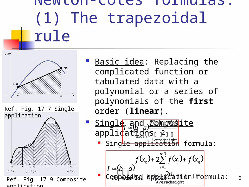
Newton-cotes formulas: (1) The trapezoidal rule

Basic idea: Replacing the complicated function or tabulated data with a polynomial or a series of polynomials of the first order (linear).

Single and Composite applications Single application formula:

Composite application formula:

Ref. Fig. 17.7 Single application

Ref. Fig. 17.9 Composite application

Height AverageWidth

2

bfafabI

Height Average

1

10

Width2

2

n

xfxfxfabI

n

n

ii

Dr. Jie Zou PHY3320 7

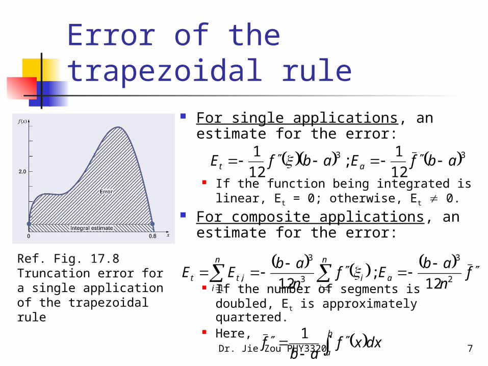
Error of the trapezoidal rule

For single applications, an estimate for the error:

If the function being integrated is linear, Et = 0; otherwise, Et 0.

For composite applications, an estimate for the error:

If the number of segments is doubled, Et is approximately quartered.

Here,

33

12

1 ;

12

1abfEabfE at

Ref. Fig. 17.8 Truncation error for a single application of the trapezoidal rule

f

n

abEf

n

abEE a

n

ii

n

iitt

2

3

13

3

1, 12

; 12

b

adxxf

abf

1

Dr. Jie Zou PHY3320 8

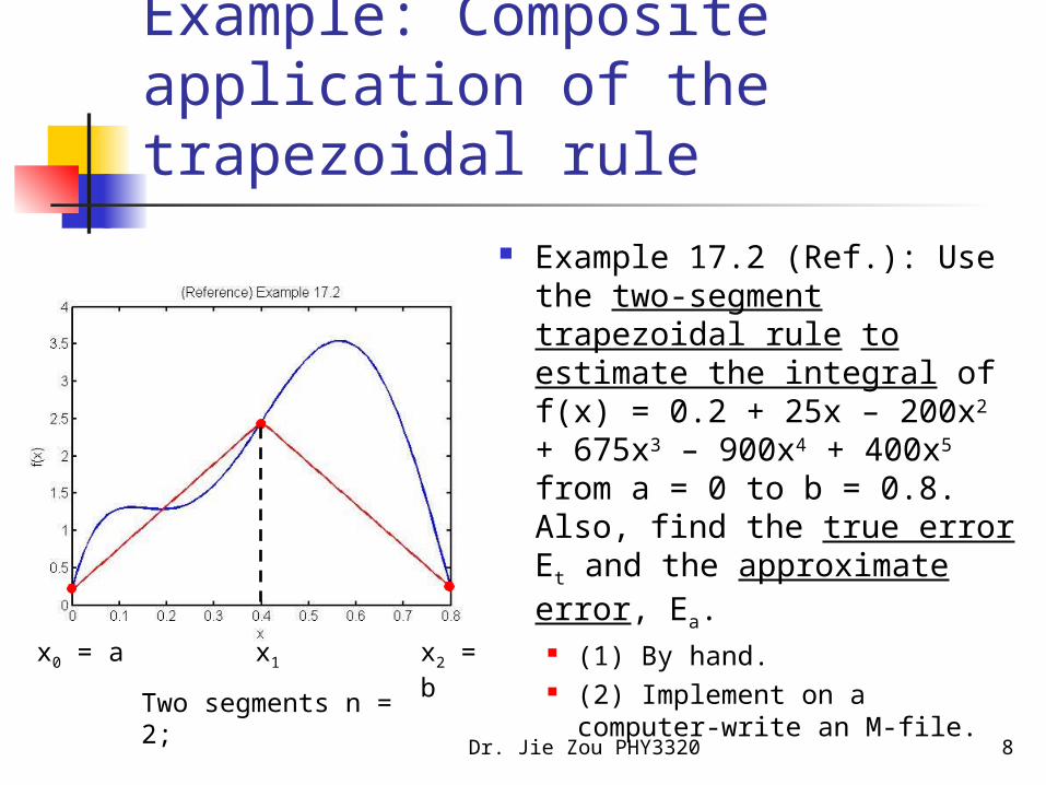
Example: Composite application of the trapezoidal rule

Example 17.2 (Ref.): Use the two-segment trapezoidal rule to estimate the integral of f(x) = 0.2 + 25x – 200x2 + 675x3 – 900x4 + 400x5 from a = 0 to b = 0.8. Also, find the true error Et and the approximate error, Ea.

(1) By hand. (2) Implement on a

computer-write an M-file.

x0 = a x1

x2 = b

Two segments n = 2;

Dr. Jie Zou PHY3320 9

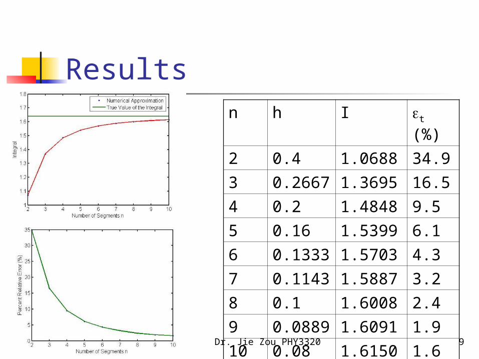
Resultsn h I t (%)

2 0.4 1.0688 34.9

3 0.2667 1.3695 16.5

4 0.2 1.4848 9.5

5 0.16 1.5399 6.1

6 0.1333 1.5703 4.3

7 0.1143 1.5887 3.2

8 0.1 1.6008 2.4

9 0.0889 1.6091 1.9

10 0.08 1.6150 1.6

Dr. Jie Zou PHY3320 10

Implementation of composite trapezoidal rule on a computer

Write an M-file called My_Trapezoidal_Rule.m to do Example 17.2.

A copy of the code will be handed out later.