Embed Size (px)
Citation preview

New Jersey Department of Environmental Protection
Site Remediation Program
DRAFT Characterization of
Contaminated Ground Water Discharge
to Surface Water
Technical Guidance
DRAFT JUNE 2015DRAF
T

Table of Contents
List of Acronyms ........................................................................................................................... iii
1.0 Intended Use of Guidance Document ....................................................................................... 1
2.0 Purpose ...................................................................................................................................... 2
3.0 Document Overview ................................................................................................................. 3
3.1 Approach for Evaluating Contaminated Ground Water Discharge to Surface Water .......... 4
3.1.1 Ground Water Remedial Investigation Approach .......................................................... 4
3.1.2 Surface Water SI and Ecological Evaluation ................................................................. 4
3.1.3 Investigation Results....................................................................................................... 4
4.0 Conceptual Models of GW-SW Interaction .............................................................................. 6
4.1 Ground Water - Stream Interaction ....................................................................................... 7
4.1.1 Ground Water and Streams Special Case: The Hyporheic Zone .................................... 8
4.2 Ground Water-Wetlands Interaction ..................................................................................... 8
4.2.1 Tidal Fluctuations .......................................................................................................... 9
4.3 Ground Water and Lake Interaction .................................................................................... 10
5.0 Site Specific Conceptual Model Development .................................................................. 11
5.1 Ground Water Flow and Discharge Parameters ................................................................. 11
5.1.1 Hydraulic Head Gradient .............................................................................................. 11
5.1.2. Aquifer Hydraulic Conductivity and Stratigraphy ...................................................... 12
5.1.3 Sediment Hydraulic Conductivity ................................................................................ 12
5.1.4 Geometry and Gradient of the Receiving Water Body ................................................. 12
5.1.5. Sediment Bedforms ..................................................................................................... 12
5.2 Modeling Tools to Help Constrain the Problem: Ground Water to Surface Water
Discharge Modeling .................................................................................................................. 12
5.3 Contaminant Fate and Transport Considerations ........................................................... 13
5.3.1 Organic compounds ................................................................................................ 15
5.3.2 Inorganic compounds .............................................................................................. 15
5.4 Special Case: Non-Aqueous Phase Liquid seeps ........................................................... 15
6.0 Characterization Methods and Tools ................................................................................. 17
6.1 Locating Ground Water Discharge Zones in Surface Water .......................................... 18
6.1.1 Remote Sensing Data Inventories ................................................................................. 18 DRAF
T

ii
6.1.2 Visual Inspections ................................................................................................... 18
6.1.3 Temperature Surveys .............................................................................................. 19
6.1.4 Electrical Conductivity and Resistivity .................................................................. 19
6.1.5 Hydraulic Head ........................................................................................................... 19
6.2 Determining Sediment Pore Water Quality in Ground Water Discharge Zones ................ 20
6.2.1 Pore Water Sampling Frequency .................................................................................. 20
6.2.2 Pore Water Sampling Equipment and Procedures ....................................................... 20
6.3 Multi-parameter characterization tools ............................................................................... 21
6.3.1 Trident Probe ................................................................................................................ 21
6.3.2 Ultraseep ...................................................................................................................... 21
6.4 Determining Surface Water Quality at Ground Water Discharge Zones ....................... 22
7.0 Remedial Action and Performance Monitoring Program ....................................................... 23
7.1 Remedial Action Strategies for Ground water Plume Discharge ........................................ 23
7.1.1 Ground Water Plume Treatment Amendments ............................................................ 23
7.1.2 Permeable Reactive Barriers in Ground Water or Sediment ........................................ 24
7.1.3 Ground Water Containment .......................................................................................... 24
7.1.4 Monitored Natural Attenuation and Recovery ............................................................. 24
7.2 Performance Monitoring ..................................................................................................... 25
7.2.1 General Considerations for Monitoring Ground Water and Surface Interaction ......... 25
7.3 Developing a Remediation Monitoring Program ................................................................ 27
REFERENCES ............................................................................................................................. 31
Table 1: Ground Water – Pore Water – Surface Water Data Evaluation ............................. Table 1
Table 2: : Surface Water and Pore Water Assessment Methods .......................................... Table 2
Appendix A: Ground Water to Surface Water Discharge Models ............................................. A-1
Appendix B: Case Studies of Transformation Processes within the Transition Zone ............... B-1
Appendix C: Temperature Measurement Equipment ................................................................ C-1
Appendix D Conductivity and Resistivity ................................................................................ D-1
DRAF
T
iii
List of Acronyms
DNAPL dense non-aqueous phase liquid
DTS fiber-optic distributed temperature sensing
ESC ecological screening criteria
ESNR Environmentally Sensitive Natural Resource
EETG NJDEP Ecological Evaluation Technical Guidance Document
FSPM NJDEP Field Sampling Procedures Manual (FSPM)
GPS global positioning system
GW ground water
GWQS N.J.A.C. 7:9C-1 et seq. The NJDEP Ground Water Quality Standards
GWRS N.J.A.C. 7:26D-2 et seq. The NJDEP Minimum Ground Water Remediation
Standards
GWTG The NJDEP Ground Water Technical Guidance: Site Investigation, Remedial
Investigation, Remedial Action Performance Monitoring
LNAPL light non-aqueous phase liquid
MNR Monitored Natural Recovery as described in the US Department of Defense
Monitored Natural Recovery at Contaminated Sediment Sites guidance document
NAPL non-aqueous phase liquid
RI Remedial Investigation as defined in the TRSR
SI Site Investigation as defined in the TRSR
SW surface water
SWQS N.J.A.C. 7:9B, The NJDEP Surface Water Quality Standards
SWRS N.J.A.C. 7:26D-3 et seq. The NJDEP Minimum Surface Water Remediation
Standards
TRSR N.J.A.C. 7:26E-1 et seq. The NJDEP Technical Requirements for Site
Remediation
DRAF
T

1.0 Intended Use of Guidance Document This guidance is designed to help the person responsible for conducting the remediation to comply
with the Department's requirements established by the Technical Requirements for Site Remediation
(Technical Rules), N.J.A.C. 7:26E, dated May 2012. This guidance will be used by many different
people involved in the remediation of a contaminated site; such as Licensed Site Remediation
Professionals (LSRP), Non-LSRP environmental consultants and other environmental professionals.
Therefore, the generic term “investigator” will be used to refer to any person that uses this guidance
to remediate a contaminated site on behalf of a remediating party, including the remediating party
itself.
The procedures for a person to vary from the technical requirements in regulation are outlined in the
Technical Rules at N.J.A.C. 7:26E-1.7. Variances from a technical requirement or departure from
guidance must be documented and adequately supported with data or other information. In applying
technical guidance, the Department recognizes that professional judgment may result in a range of
interpretations on the application of the guidance to site conditions.
This guidance supersedes previous DEP guidance issued on this topic. Technical guidance may be
used immediately upon issuance. However, the Department recognizes the challenge of using newly
issued technical guidance when a remediation affected by the guidance may have already been
conducted or is currently in progress. To provide for the reasonable implementation of new technical
guidance, the Department will allow a 6-month “phase-in” period between the date the technical
guidance is issued final (or the revision date) and the time it should be used.
This guidance was prepared with stakeholder input. The following people were on the committee who
prepared this document:
Dan Cooke, AMEC Foster Wheeler Environment & Infrastructure, Inc.
Bill Cordasco, TRC Environmental Corporation
Scott Drew, Geosyntec
Nancy Grosso, DuPont Corporate Remediation Group
Bill Hanrahan, NJDEP, Bureau of Environmental Measurements and Site Assessment
Ward Ingersoll, NJDEP, Bureau of Environmental Measurements and Site Assessment
Jill Monroe, NJDEP, Bureau of Ground Water Pollution Abatement
Christina Page, NJDEP, Bureau of Inspection and Review
John Ruhl, NJDEP, Bureau of Environmental Evaluation and Risk Assessment
Terrance Stanley, Langan Engineering and Environmental Services, Inc.
DRAF
T
2
2.0 Purpose The purpose of this document is to provide guidance for the identification, characterization and
monitoring of contaminated ground water impacts to surface water bodies and thereby assist in
complying with the Technical Requirements for Site Remediation (N.J.A.C. 7:26E-1 et seq.).
Specifically, this guidance provides tools for complying with the following rules when
contaminated ground water has the potential to impact surface water:
7:26E-3.6(a); how to determine if there is a potential that ground water contamination
from a site has reached surface water
7:26E-4.4(a)1, how to determine if ground water contamination is a source of
contamination in surface water and the migration pathway
7:26E-5.2(a)2 considerations for developing and implementing a monitoring program to
effectively monitor the performance of the remedial action for contaminated ground
water discharges to surface water
DRAF
T

3
3.0 Document Overview This guidance provides tools and methods to characterize the ground water to surface water
pathway to obtain the data necessary to evaluate contaminated ground water discharges to
surface water. The document describes the following:
an approach for conducting an investigation of contaminated ground water discharges to
surface water
conceptual models of the ground water migration to surface water pathway
tools that are available to investigate the pathway
remedial action performance monitoring considerations
New Jersey has flowing surface water bodies that range from intermittent streams to large river
systems. A significant number are tidally influenced. The state also has ponds, lakes, and miles
of coastal and estuarine water resources. Freshwater and saltwater wetland areas are also found
near most surface waters. New Jersey’s surface water systems are located in a wide variety of
geologic settings, from the glaciated regions of northern New Jersey to the coastal plain of
southern New Jersey, and include ecologically unique and/or protected areas such as the
Pinelands and the Highlands regions.
Being a densely populated state with a long development history, surface water has been used for
recreation, water supply and wastewater management. While some surface water systems are
relatively un-impacted, others have experienced greater degrees of change due to agriculture,
suburban and urban development, industrial manufacturing, air pollution, etc. that affect their
quality. Some contaminants affecting surface water come from overland flow or storm water
collection systems. Others come from point source discharges (e.g., wastewater effluent) or from
contaminated ground water that discharges to surface water. It is the latter discharge type that is
the focus of this document.
Sources of ground water contamination are highly variable. Some sources may be from a single
leaking residential heating oil tank, and others may be from a petrochemical complex in
operation since before World War I. The end result is that the contaminants identified in ground
water can be significantly different between sites in terms of plume size (horizontal and vertical
extent), magnitude (contaminant concentrations), chemical composition (classes of
contaminants), and chemical complexity (single source or multiple sources).
Based on the variability of ground water hydrogeology and surface water hydrology across the
state, the ground water to surface water migration pathways for each site will be unique. The
magnitude of impact from a contaminant discharge to surface water will also vary, and will be
affected by surface water flow, sediment characteristics and ecological communities at the
discharge zone. Therefore, for each site, a site-specific investigation is required to characterize
the contaminated ground water discharge and identify adverse impacts to surface water quality,
sediment, and ecological receptors associated with that discharge.
DRAF
T

4
3.1 Approach for Evaluating Contaminated Ground Water Discharge to Surface Water
When ground water contamination above the Surface Water Quality Standards is identified close
to surface water, the contaminated ground water to surface water discharge zone should be
characterized, and a Site Investigation (SI) of surface water and ecological receptors is required.
A conceptual model that incorporates physical, hydraulic, and chemical aspects of the system
should be developed to support a field investigation approach. The objective of the investigation
is to identify the location(s) of the contaminated ground water discharge zone(s) and determine if
the ground water contaminant migration pathway to surface water is complete. Any impact to
surface water, sediment, and ecological receptors will need to be characterized in accordance
with the Technical Requirements for Site Remediation (TRSR) and the Ecological Evaluation
Technical Guidance (EETG). The investigator needs to be familiar with the provisions of the
SWQS at N.J.A.C. 7:9B-1.5 and 1.14 that are incorporated into the Remediation Standards,
including the antidegredation policies and surface water classifications that may influence
remedial actions in different parts of the state. The goal of the SWQS is to restore waters that
exceed criteria, maintain waters that are better than criteria, and preserve those waters
determined to be of outstanding natural resource value.
3.1.1 Ground Water Remedial Investigation Approach
Pursuant to 7:26E-4.3(a)4 and 4.3(b)1, the person responsible for the remediation shall delineate
the horizontal and vertical extent of ground water contamination. Technical guidance concerning
delineation of ground water contamination is available in the Department’s GWTG.
When there is the potential that a ground water contaminant plume discharges to surface water,
the discharge zone(s) must be located so that surface water, sediment pore water, and sediment
sampling must be biased to the area that is most contaminated in accordance with the SI
requirements for all media in the TRSR N.J.A.C. 7:26E-3.3(a). The discharge area should be
located using the methods and tools outlined in Section 6 of this document.
3.1.2 Surface Water SI and Ecological Evaluation
After the contaminated ground water discharge zone has been located, surface water samples
must be collected from the area to assess potential surface water impacts. In addition, sediment
and sediment pore water should also be sampled (see NJDEP EETG). The most contaminated
portion of the discharge zone will be targeted for sampling to assess worst case conditions.
Sampling locations should be selected in accordance with the TRSR, this guidance and the
guidance provided in the Department’s EETG.
3.1.3 Investigation Results
Surface water, sediment and sediment pore water sample results are compared to the applicable
Remediation Standards (N.J.A.C. 7:26D-1 et seq.) and Ecological Screening Criteria (ESC).
Where standards or criteria are exceeded, a remedial investigation of surface water or ecological
receptors is required in accordance with the TRSR. Guidance on complying with the
Department’s Remediation Standards and Criteria may be found in the Department’s Technical
Guidance for the Attainment of Remediation Standards and Site-Specific Criteria and the EETG. DRAF
T

5
Where surface water or ecological samples do not exceed the applicable SWRS or ESC, no
remedial investigation is required. However, the ground water contaminant plume and surface
water will need to be monitored to ensure that contaminated ground water does not impact
surface water at a future time as discussed in Section 7. Monitoring should continue until there is
no longer the potential for ground water contamination to impact surface water. Table 1 provides
a general outline for the evaluation of ground water, pore water and surface water data.
DR
AFT

6
4.0 Conceptual Models of GW-SW Interaction The development of an investigation approach should begin with a sound ground water to
surface water conceptual model. Guidance on developing a conceptual model of site
hydrogeology may be found in the Department’s Ground Water Technical Guidance at
http://www.nj.gov/dep/srp/guidance/srra/gw_inv_si_ri_ra.pdf . The initial conceptual model of
ground water surface water interaction should begin with a desktop review of available data for
the location of interest. General resources include the following:
o Topographic Map http://topomaps.usgs.gov/
o Geologic Map http://www.state.nj.us/dep/njgs/pricelst/geolmapquad.htm
o Stratigraphic Cross Section: Use data from site related and nearby boring logs
http://datamine2.state.nj.us/DEP_OPRA/OpraMain/categories?category=WS+We
ll+Permits
o Estimate of Hydraulic Conductivity: site specific tests or estimated from the New
Jersey Geological Survey hydro database
http://www.state.nj.us/dep/njgs/geodata/dgs02-1.htm
o Real time ground water and surface water data: http://nj.usgs.gov/
o Streamflow: http://nj.usgs.gov/
Several conceptual models of ground water surface water interaction will be briefly discussed in
this section. For a more comprehensive discussion of ground water surface water conceptual
models, including extensive illustrations, see the USGS Circular 1139 “Ground Water and
Surface Water A Single Resource” available at http://pubs.usgs.gov/circ/circ1139/. In addition,
Conant (2004) outlines the following 5 types of ground water interaction with surface water
based on sediment and aquifer characteristics:
Short circuit discharge: An area where natural or man-made conduits exist in the
subsurface deposits that allow ground water from depth to rapidly reach the surface water.
High Discharge: Areas of preferred ground water flow where streambed deposits with
high hydraulic conductivity connect with aquifer deposits with high hydraulic
conductivity.
Low to Moderate Discharge: Areas where low to medium hydraulic conductivity
streambed deposits are present relative to similar aquifer deposits or there is a low
hydraulic gradient or both.
No Discharge: Areas where the hydraulic gradient between streambed deposits and
aquifer is zero and no discharge to surface water occurs.
Recharge areas: Areas where the hydraulic gradient between the streambed and aquifer is
downward (surface water is recharging the aquifer).
DRAF
T

7
4.1 Ground Water - Stream Interaction Ground water interacts with streams depending on geologic and hydrologic conditions. Ground
water flow can infiltrate through a streambed and become surface water and vice versa. When
the elevation of a stream is lower than adjacent ground water elevations, ground water will flow
to the stream (a gaining stream). Where surface water elevations are greater than nearby ground
water elevations and surface water recharges ground water (a losing stream). Gaining and losing
conditions can vary both spatially and over time. Spatially, a stream may be gaining along one
stretch and transition to losing at another. This may be caused by changing geologic terrain or
ground water withdrawal wells. Temporal changes in gaining or losing conditions may be due to
rainfall events which increase stream stage relative to ground water elevation or droughts which
can decrease stream stage relative to ground water elevation.
The scale of gaining and losing can also vary. An entire reach of a stream may be considered
typically either gaining or losing. Conversely, a stream may actually be losing along small
portions of its path such as in the outside of a meander where swift running surface water may
rise slightly above the adjacent ground water. Under certain conditions, one side of a stream may
be gaining while losing on the opposite side. Identifying gaining or losing conditions along a
stream reach influences the potential contaminant flux from ground water to surface water.
Figure 2. Gaining Streams: Gaining streams receive water from the ground-water system (A). This can be determined from water-table contour maps because the contour lines point in the upstream direction where they cross the stream (B)
Figure and Text courtesy of the U.S. Geological Survey (U.S.G.S. 1998)
Figure 1. Losing Stream: Losing streams lose water to the ground-water system (A). This can be determined from water-table contour maps because the contour lines point in the downstream direction where they cross the stream (B)
Figure and Text courtesy of the U.S. Geological Survey (U.S.G.S. 1998)
DRAF
T

8
Figure 3. Hyporheic Zone: Surface-water exchange with ground water in the hyporheic zone is associated with abrupt changes in
streambed slope (A) and with stream meanders (B).
Figure and Text courtesy of the U.S. Geological Survey (U.S.G.S. 1998)
Natural losing stream conditions are rare in New Jersey. However, large scale losing stream
conditions exist in coastal plain streams and rivers where ground water is depleted as the result
of pumping for municipal drinking water supply. Temporary “losing” conditions caused by
natural events, e.g., associated with storm flows discharging to unsaturated bank soils, do not
result in a net reversal of flow from streams to adjacent aquifers.
4.1.1 Ground Water and Streams Special Case: The Hyporheic Zone The subsurface zone where stream water flows through short segments of its adjacent bed and
banks is referred to as the hyporheic zone (USGS, 1998). Ground water and surface water
mixing in this zone occurs in coarse-grained higher permeability sediments. Because of this
mixing, the chemical and biological character of the hyporheic zone may differ from
adjacent surface water and ground water (USGS, 1998). Within the hyporheic zone a complex
interaction between biology, geology and hydrology may take place creating unique ecological
conditions that do not exist in either surface water or ground water. The zone provides a porous
matrix where ground water flux and mass exchange occur, in addition to performing important
biological functions. The size and geometry of hyporheic zones vary greatly with respect to the
specific features of a fluvial system. With respect to the ground water to surface water migration
pathway, the hyporheic zone provides a matrix where biogeochemical effects can be evaluated
along the path of ground water flow. Conditions in the hyporheic zone can be very dynamic,
exhibiting both temporal and spatial variation depending upon specific components of the
drainage basin. For more information on the hyporheic zone see USGS (1998), USEPA (2008)
and Environment Agency UK (2005).
4.2 Ground Water-Wetlands Interaction Wetland hydrology may be sustained by ground water discharging as surface seepage or present
as a perennially shallow water table. Wetlands may also be sustained by surface water,
precipitation and topographic depressions or by a combination of these influences. It should be DRAF
T
9
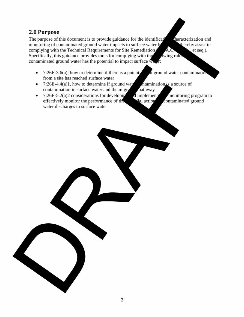
noted that wetlands do not always occupy low points and depressions, seepage wetlands can be
present on slopes USGS (1998).
4.2.1 Tidal Fluctuations
Tidal fluctuation affects wetland hydrology in coastal wetlands and riverine aquatic
environments by influencing the direction of ground water/surface water exchange. The extent of
tidal influence on ground water/surface water exchange depends upon several factors including:
the hydraulic gradient between the adjacent aquifer and wetland, lithology, tidal range, or nearby
ground water withdrawals. Although local effects may be significant, the overall net ground
water flow in aquifers proximal to tidal water bodies is seaward. However, a careful evaluation
of tidal effects is needed in such areas to determine local ground water flow patterns and the
likely route of associated contaminant flow to the surface water body.
Figure 4. Wetlands and Ground Water
The source of water to wetlands can be from ground-water discharge where the land surface is underlain by complex ground-water
flow fields (A), from ground-water discharge at seepage faces and at breaks in slope of the water table (B), from streams (C), and
from precipitation in cases where wetlands have no stream inflow and ground-water gradients slope away from the wetland (D).
Figure and Text courtesy of the U.S. Geological Survey (U.S.G.S. 1998)
DRAF
T
10
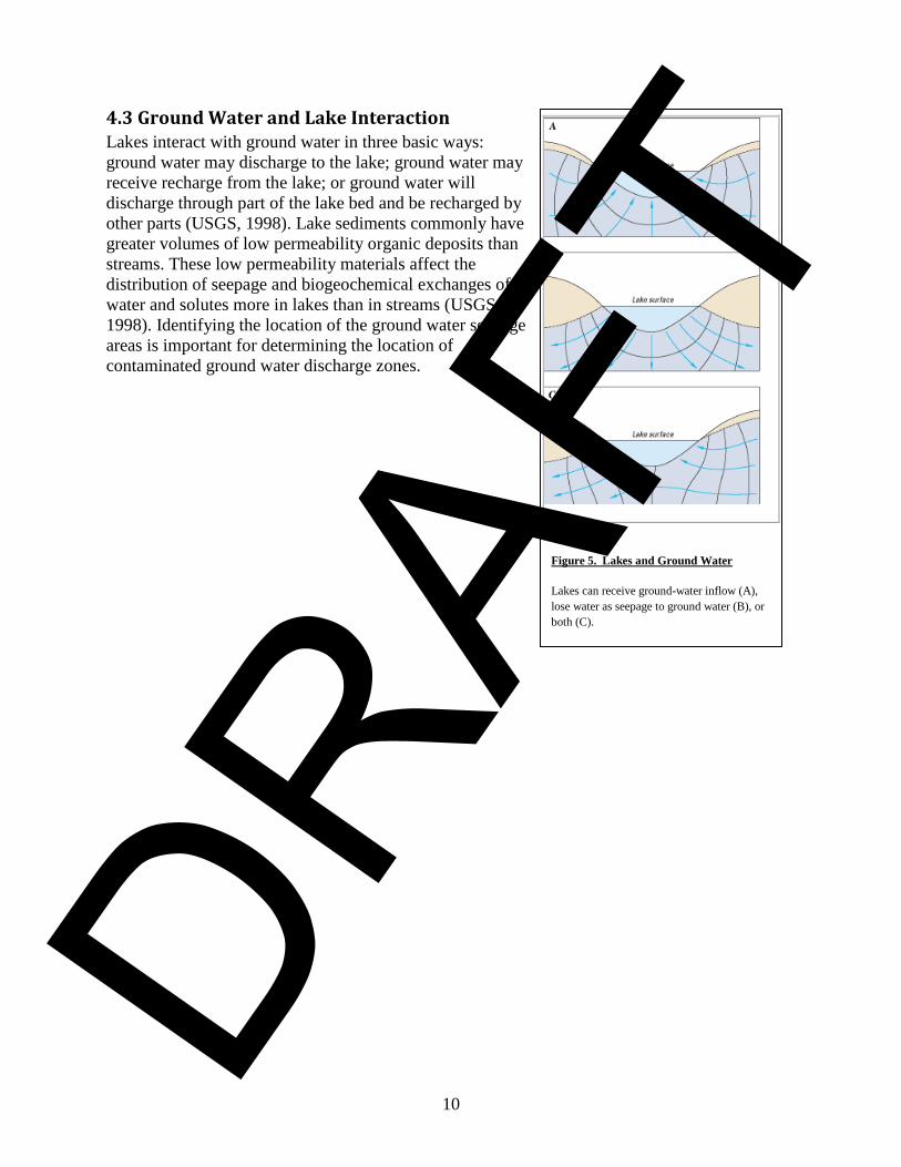
Figure 5. Lakes and Ground Water
Lakes can receive ground-water inflow (A),
lose water as seepage to ground water (B), or
both (C).
Figure and Text courtesy of the U.S.
Geological Survey (U.S.G.S. 1998)
4.3 Ground Water and Lake Interaction Lakes interact with ground water in three basic ways:
ground water may discharge to the lake; ground water may
receive recharge from the lake; or ground water will
discharge through part of the lake bed and be recharged by
other parts (USGS, 1998). Lake sediments commonly have
greater volumes of low permeability organic deposits than
streams. These low permeability materials affect the
distribution of seepage and biogeochemical exchanges of
water and solutes more in lakes than in streams (USGS,
1998). Identifying the location of the ground water seepage
areas is important for determining the location of
contaminated ground water discharge zones.
DRAF
T

11
5.0 Site Specific Conceptual Model Development A conceptual site model (CSM) is a representation of the conditions and the physical, chemical
and biological processes that control the transport, migration and potential impacts of
contamination (in soil, air, ground water, surface water and/or sediments) to human and/or
ecological receptors (NJDEP, 2011- technical guidance for Conceptual Site Models). A
technically sound conceptual model incorporates the important physical, biogeochemical, and
chemical system parameters and integrates those parameters with consideration of the dynamic
environment in space. The development of a CSM helps ensure consistency of a particular
interpretation of the existing data set. The presentation of a CSM can be diagrammatic or a
written description. For ground water and surface water interaction, diagrams and cross sections
are often developed parallel to the direction of ground water flow as part of the ground water
discharge to surface water conceptual model to illustrate important contaminant fate and
transport pathways and processes.
5.1 Ground Water Flow and Discharge Parameters Synoptic water table and river stage elevation measurements are used to determine whether a
stream is gaining or losing. Although these measurements are critical for determining general
ground water flow direction, other parameters can affect when and where ground water
discharges to (or is recharged by) surface water on a local scale. The rate of ground water to
surface water flow can vary from slow diffuse seepage to rapid concentrated flow. Parameters
that affect the nature of the exchange at the ground water discharge to surface water transition
zone include the following:
ground water hydraulic gradient and aquifer hydraulic conductivity
stream hydraulic gradient and stream bed hydraulic conductivity
hydraulic gradient between ground water and surface water
aquifer and stream bed sediment permeability
geometry of stream bed at or near the ground water discharge area
sediment bedforms
5.1.1 Hydraulic Head Gradient
Ground water flows from areas of high hydraulic head to areas of lower hydraulic head. The
quantity of ground water discharge (i.e., flux) to and from surface water bodies can be
determined for a known aquifer cross section using Darcy’s equation by multiplying the
hydraulic gradient by the hydraulic conductivity and the cross sectional area of the discharge.
If necessary, more detailed evaluations can be made through sensitivity analysis and/or
mathematical modeling. Hydraulic factors that can affect ground water volumetric and/or
constituent mass flux, such as tidal variations in the receiving water, should also be considered.
Hydraulic head and surface water stage vary seasonally; therefore, ground water to surface water
discharge patterns can vary in magnitude and direction throughout the year. Examples of
seasonal influences include ground water mounding due to enhanced recharge or ground water
depressions caused by evapotranspiration during the growing season. Seasonal conditions should
be considered when head measurements are taken and interpreted.
DRAF
T

12
5.1.2. Aquifer Hydraulic Conductivity and Stratigraphy
Geologic units with different hydraulic conductivities also have variable spatial ground water
discharge (seepage distribution) in surface water beds. For example, a highly permeable sand
layer within an aquifer consisting largely of silt transmits water preferentially into surface water
as a subaqueous spring. An extreme case demonstrating this process is preferential flow in karst
terrain or fractured bedrock.
5.1.3 Sediment Hydraulic Conductivity
Varying hydraulic conductivities of bed sediments can affect where ground water discharges to
the surface water body. If a sediment bed consists of one sediment type such as sand, ground
water discharge is generally greatest at the shoreline and decreases in a nonlinear pattern away
from the shoreline toward the middle of the steam (USGS, 1998). However, if the sediment bed
is mantled by a finer grained material such as silt or “river mud,” most ground water seepage will
occur in those areas with higher permeability. For streams with very coarse bed sediments,
hyporheic flow may occur.
5.1.4 Geometry and Gradient of the Receiving Water Body
Meandering streams are one example of stream flow in and out of porous media (e.g., alluvial
plain, floodplain deposits). Stream meanders and regions of locally high slope drive the
exchange process between stream water and pore water. Woessner (Woessner, 1998) studied the
flow paths of a meandering mountain stream that lies on sediment of fine sand and some gravel
layers. At high stream discharge, flow is primarily in a downstream direction; at low discharge,
more flow occurs in and out of the stream bank. Other considerations when developing the
conceptual model are the size of the receiving body, surface water flow characteristics and the
bathymetry of the surface water body.
5.1.5. Sediment Bedforms
In some cases, the morphology of the sediment bed influences the hydraulics of a system. Dunes
and ripples similar to those seen in natural river deposits were reproduced in flume studies. The
studies show that as stream flow proceeds over a dune, flow is induced under the bedform in
such a way that surface water can flow into the porous media (bedform) and out into the stream
again (Thibideaux and Boyle, 1987). For gravel, the depth of this pumping exchange can extend
well below the base of the dune or ripple. Pumping is defined as the exchange due to advective
pore water flow. Smaller pore spaces in sand streambeds restrict stream pore water flow coupling
to a more shallow depth in the dune.
5.2 Modeling Tools to Help Constrain the Problem: Ground Water to Surface
Water Discharge Modeling A model is “any device that represents an approximation of the field situation” (Anderson and
Woessner, 1992). While models are useful tools, they do not substitute for sampling to characterize
the ground water to surface water pathway. The use of a model to predict a resultant surface water
receptor impact does not approve the discharge of contamination from ground water to surface
water. A model result due to dilution will not substitute for the determination of compliance with
the remediation standards - surface water (human health and aquatic health criteria) as identified in
the Department’s Attainment Guidance. . The investigation and site sampling must show that DRAF
T
13
model assumptions and predicted outcome are representative of actual site conditions and
groundwater-surface water interaction
In general, modeling requires the investigator to focus on the most important aspects of the field
situation and can result in more efficient data collection and remedial action. There are two main
types of mathematical models that are derived from a conceptual site model: analytical models
and numerical models. Analytical models typically consist of a mathematical equation for which
the user supplies the required input values and then manually (hand calculator or spreadsheet)
calculates the result. Numerical models are more computationally complex and often require
extensive input data and are processed using a computer. The advantage of numerical models
over analytical models is that they can be used to simulate complex site conditions.
An overview of several models, including general advantages and limitations, that can be used
for simulating discharge to surface water and ground water-surface water exchange is presented
in Appendix 1.
5.3 Contaminant Fate and Transport Considerations Base flow conditions exist when ground water provides all inflow to a stream channel or lake
(i.e., no runoff). The transformation of ground water plume contaminants as they migrate
between the aquifer and surface water environments have not been studied at great length
because they are difficult to observe and measure. The transition from ground water to surface
water may be considered to occur in one or more of the following three broader zones:
Surface Water Column
This can include the near-field (close to the area of ground water discharge) and far-field
surface water (some distance downstream of the discharge area where substantial mixing
may have occurred).
Biologically Active Zone
This zone is generally located in surficial sediments, extending approximately 10
centimeters (cm) beneath the sediment bed. The biologically active zone is generally
considered the exposure point for benthic organisms.
Transition zone
This is the zone where physical mixing and geochemical interaction of ground water and
surface water may occur. The transition zone can be important in some settings (e.g.,
rivers, streams, lakes, wetlands) because it can store and retain nutrients and retain
ground water contaminants through adsorption or biological and chemical
transformations. The transition zone can be an important natural attenuation zone for
contaminated ground water. In some cases, the transition zone and the biologically active
zone can be the same zone or intersect one another.
If the transition zone is at a different redox state than the discharging ground water, the mixing of DRAF
T

14
redox conditions can affect the discharging contamination plume. Variations in redox chemistry,
surface water chemistry, and microbial communities can change along gradients determined by
ground water and surface water mixing. In some cases, these gradients are very steep over a
relatively small distance. Due to these gradients, the dominant contaminant fate pathways may
change. Conditions in the transition zone may be conducive to transforming or destroying
contaminants, resulting in the attenuation of contaminant plumes at or before they reach the
sediment surface water interface. Consequently, a ground water discharge from a contaminated
plume into surface water does not necessarily translate to an impact to surface water quality. The
role of the transition zone should be identified when evaluating the potential environmental fate
of the contaminants of concern.
The processes responsible for in-situ contaminant attenuation can be divided into the following
three categories:
1. Transformative: Transformative processes can be biotic or abiotic and represent a net
chemical change and accompanying changes in contaminant toxicity or mobility. Examples
of such processes are microbially mediated dechlorination reactions found in reducing
environments. However, transformative processes do not always result in a toxicity decrease.
For example, when perchloroethylene (PCE) degrades to vinyl chloride or mercuric ions
biotransform to methylmercury, the products of the transformative reaction are more toxic
than the parent contaminants.
2. Destructive: Destructive processes can be biotic or abiotic; however, these processes
represent a net mineralization (i.e., breakdown of the compound to carbon dioxide, water,
and other inorganic metabolites). In this way, transformative changes can be part of a
sequential series of reactions leading to destructive processes. For example, the sequential
reductive dechlorination of chlorinated ethenes to vinyl chloride can be followed by the
oxidation of vinyl chloride to ethene and chloride under iron-reducing conditions.
3. Nondestructive/Retarding: Nondestructive/retarding attenuation processes are often the result
of physical environmental characteristics such as organic carbon content and include
reversible processes that affect contaminant transport through the transition zone (e.g.,
adsorption, precipitation/dissolution, ion exchange).
Under in-situ conditions, it is possible for all three of these mechanisms to play a role in
contaminant fate and transformation.
• Organic-rich bottom sediment and mud typically produce highly reducing conditions and
have a high sorption capacity for organic contaminants. When a high redox (oxidizing
conditions) plume enters a transition zone characterized by low redox (reducing conditions),
a zone of accelerated biodegradation of highly chlorinated compounds may result.
• Surface water flow through coarse bed material sometimes can maintain aerobic conditions,
even when discharging ground water is anaerobic. When a low redox plume enters a zone of
high redox (oxidizing) conditions, a change in degradation pathways from sequential
reductive dechlorination to anaerobic and/or aerobic oxidation of the lower chlorinated
daughter products may be produced by transformative reductive dechlorination processes. DRAF
T

15
Tidal pumping can also deliver oxygenated water to the aquifer potentially enhancing
oxidation of contaminants.
Not all contaminant transformations are desirable and, if the ground water is actively loading the
transition zone with contaminants, it may cause the sediments to become reservoirs of
contamination (Conant, 2000). Examples of transformation processes within the transition zone
are presented in Appendix 2.
5.3.1 Organic compounds Biodegradation of organic compounds vary under differing redox conditions. Anaerobic
degradation of certain compounds such as chlorinated ethenes is well established. There are
numerous documented cases of aerobic degradation of other organics such as petroleum
hydrocarbons. Refer to the Department’s Technical Guidance on Monitored Natural Attenuation
(2012) for more discussion.
Individual compounds can degrade with differing efficiencies depending on the specific
anaerobic redox conditions (i.e., iron reduction, sulfate reduction, methanogenesis) or aerobic
conditions. Therefore, when developing the contaminant fate conceptual model, it is important to
identify the range of redox conditions present within the transition zone.
5.3.2 Inorganic compounds In the case of a ground water plume with inorganic contaminants, chemical reactions at the
transition zone may also occur. Most metals are in a dissolved state at low pH and anaerobic
conditions, and form a precipitate at higher pH or aerobic conditions. Anaerobic ground water
containing dissolved metals discharging into an aerobic streambed or stream channel can result
in precipitation of metals. Petroleum hydrocarbon plumes frequently contain dissolved iron and
precipitation of the iron in surface water is not uncommon. Additionally, if ground water is
characterized by low pH and high dissolved metals, infiltration of high pH seawater could cause
precipitation of metals from solution.
The presence of a sulfate-reducing zone in the transition zone intercepting a low-redox ground
water plume containing soluble reduced metals can result in metal contaminant attenuation by
metal sulfide precipitation. An example of this process is the treatment of acid mine drainage
through pH neutralization and insertion of a sulfate-reducing zone (usually by addition of a
source of organic matter and sulfate) to intercept the contaminant plume. Under anoxic
conditions, the metal sulfide precipitates should be effectively immobilized. However, if the
redox conditions in the transition zone were to change, the metal precipitates can become
oxidized and the metal contaminants remobilized.
5.4 Special Case: Non-Aqueous Phase Liquid seeps The investigation and evaluation of NAPL seeps into waterways adjacent to contaminated
underground storage tanks and above ground storage tanks have become an area of specific
attention in New Jersey. Removing the free product source will reduce mass loading of
contamination to ground water, however, residual contamination in the aquifer may discharge to
surface water. Depending on the hydrogeological setting, continued investigation and/or further
remedial measures may be warranted DRAF
T

16
The initial slug of contamination that reaches a water body through a preferential pathway can be
trapped in the soil matrix of a stream bank or river bank. The continued release of NAPL at the
may occur in the form of NAPL seeps. Specific concern arises during storm events when
flushing of the aquifer matrix can result in increased seepage rates at the bank.
Depending on the surface water classification and use, NAPL seeps may present a direct contact
concern to human health or ecological impact. Site specific evaluation should be undertaken to
determine the significance of the migration and exposure pathways.
DRAF
T

17
6.0 Characterization Methods and Tools A variety of methods and equipment have been developed to identify the location of ground
water discharge zones in surface water and to evaluate the quality of ground water, sediment
pore water, and surface water. Multiple lines of evidence should be evaluated to determine if
contaminated ground water is discharging to surface water. The investigation of contaminated
ground water discharge to surface water may be approached as follows:
Determine the Location of GW Discharge Zones in SW
o Examination of Existing Information
Hydrogeology
Ground Water Plume Orientation Relative to the Surface Water Body
Hydraulic Head
o Reconnaissance and Investigation
Visual Inspection
Seeps/visual contamination
Thermal measurements
Conductivity and Resistivity Measurements
Determine the Quality of Sediment Pore Water in the areas identified as potential
contaminated GW Discharge Zones
o Screening Techniques
o Laboratory Chemical Analysis; and
Determine SW Quality at GW Discharge Zones
o Screening Techniques
o Laboratory Chemical Analysis
The methods selected to evaluate the GW-SW migration pathway should reflect site-specific
factors including:
Hydrogeologic setting (aquifer properties, ground water flow direction, etc.)
Anthropogenic influences (fill, ground water diversion structures, buried utilities, etc.)
and
Surface water hydrology (drainage pattern, stream morphology, tidal influence
seasonality, etc.)
The following sections summarize methods described in the NJDEP FSPM, the NJDEP EETG or
that have been shown to be effective in peer reviewed literature. The discussion of the methods
and equipment presented here is not exhaustive. NJDEP, USEPA, USGS and peer reviewed
sources should be consulted for greater detail, and for technology updates and emerging
technologies. Table 1 provides a brief description of each assessment technology identified in the
following sections and includes references for further information along with respective pros and
cons.
An evaluation of methods and techniques was conducted by Kalbus (2006) and includes an
extensive reference list. The article is available at the following link: http://www.hydrol-earth-DRAF
T
18
syst-sci.net/10/873/2006/hess-10-873-2006.pdf. The USGS also operates a National Research
Program concerning “Hydrologic and Chemical Interactions between Surface Water and Ground
Water” at http://water.usgs.gov/nrp/science.php?sciArea=Groundwater-
Surface%20Water%20Interactions. The program presents reports and methods to document
ground water/surface-water interaction and is testing new field methods and models to evaluate
those interactions.
6.1 Locating Ground Water Discharge Zones in Surface Water A number of noninvasive methods based on visual and physicochemical properties are available
for surveying areas to locate ground water discharge zones. Multiple lines of evidence may be
necessary and will be contingent upon the size and depth of the water body.
6.1.1 Remote Sensing Data Inventories Review of existing aerial imagery including; high resolution satellite imagery, black and white
aerial photographs, color aerial photographs, near infrared imagery, and infrared imagery may
reveal locations of potential ground water discharge zones. The investigator should closely
examine the imagery for drainage networks and changes in vegetation. An example of nighttime
thermal infrared imaging used to identify submarine ground water discharge is available from the
Woods Hole Oceanographic Institute at http://www.whoi.edu/page.do?pid=17135.
6.1.2 Visual Inspections Visual inspections can be performed to identify seepage areas along surface water bodies.
Indicators can include the following:
Active flow discharging from stream banks in micro-channels
Areas of algal growth or wetland vegetation in otherwise upland areas above surface
waters
Areas of stressed or dead vegetation either above or below the water line
Visible discoloration of soil along banks or sediment in the surface water body (e.g.,
natural oxides, contaminant staining, etc.)
Chemical-related sheens, foam, etc. on the water body surface
Existence of contaminant-related odors
Observation of seepage faces, defined as broad areas of saturated soil below the ordinary high-
water line, but lacking definable discharge points, may be evident during low water periods.
Discrete discharges include distinct areas of ground water discharge surrounded by otherwise dry
soils. Although seepage faces and discrete discharges are obvious target areas for sampling,
additional deeper subaqueous discharge zones may also be present. For areas affected by tides,
the visual inspection is most productive during low water/low tide conditions.
During winter months, ground water discharge points or seepage areas may be evidenced by ice
free areas in frozen water bodies caused by ground water temperatures above 0oC. Discoloration
or staining of surface water, snow, ice, or exposed sediment due to oxide/ferrihydroxide
precipitates, may be encountered along the shores of surface waters, and may be evidence of
ground water discharges and localized reducing conditions. DRAF
T
19
Depending upon the quantity and properties of the discharged contaminant(s), sheens, foam, or
odors may be present at locations where the ground water contaminant plume is discharging to
surface water.
6.1.3 Temperature Surveys
The transport of natural heat by flowing water has been used to evaluate the interaction of
ground water and surface water. The contrast in temperature can be used to detect ground water
seeps. This contrast is most evident during the winter (when comparatively warmer ground water
is discharging to colder surface water) or summer (when the temperature contrast is reversed).
By measuring the temperature of surface water and the temperature at shallow depths in
sediments, Silliman and Booth (Silliman 1993) mapped gaining and losing reaches of a stream in
Indiana. Sediment temperatures had little diurnal variability in areas of ground water inflow
because of the stability of ground water temperatures. Sediment temperatures had much more
variability in areas of surface water flow to ground water because they reflected the large diurnal
variability of temperature in the surface water. This approach is useful for determining flow
direction. Lapham (USGS 1989) used sediment temperature data to determine flow rates and
hydraulic conductivity of the sediments based on fundamental properties of heat transport.
Equipment that may be used to determine temperature variation includes the following:
Thermal imaging cameras
o Thermal Infrared Multispectral Scanner (TIMS)
o Forward Looking Infrared Cameras (FLIR)
Thermometers, Thermocouples, and Thermistors
Fiber-Optic Surveys
This equipment is described further in Appendix 3.
6.1.4 Electrical Conductivity and Resistivity
Electrical conductivity of earth materials including soil, ground water and surface water varies
with the physicochemical characteristics of each medium. Ground water flowing into surface
water can sometimes be detected if its natural or altered electrical conductivity is measurably
different from that of the receiving waters. for example, where ground water discharges to saline
surface waters or where ground water contains contaminants (such as dissolved metals) that
increase its conductivity.
In addition, resistivity measurements may be used to determine the location of ground water
flowing into surface water. Detail on using conductivity and resistivity measurements is included
in Appendix 4.
6.1.5 Hydraulic Head
Piezometers may be used to identify gaining and losing areas within a surface water body by
comparing water levels adjacent to streams during base flow conditions. The screened interval of
the piezometers should be selected based on soil characteristics and lithology, and water levels
observed in open boreholes or temporary wells advanced in areas proximal to the stream. Water
level elevation data should be collected during base flow conditions after several days of dry DRAF
T

20
weather to avoid measuring temporary increases in ground water elevation from precipitation
events. Periodic depth to water measurements can be made in the piezometers while synoptic
readings of water levels are made in stilling wells installed within the stream or on the
immediately adjacent stream bank. Consistently higher elevations in the stream versus the
adjacent wells indicate losing stream conditions, whereas the reverse condition indicates gaining
stream conditions.
Hydraulic head can also be measured using a manometer board, or a potentiomanometer (a
differential pressure gauge) hooked in line between the piezometer and a stilling well (or current
damper) on the stream bed. Gaining is indicated when the hydraulic gradient is positive (USGS,
2005; USEPA, 2008).
6.2 Determining Sediment Pore Water Quality in Ground Water Discharge
Zones Sediment and pore water sampling may be conducted to delineate the extent of the contaminated
ground water discharge areas. A variety of sampling equipment exists for the collection of pore
water samples, as described further in this section and in Table 1. Note that elevated pore water
concentrations may be due to ground water discharge or it may be due to partitioning of
constituents from contaminated sediments. It is important to develop the conceptual model to the
extent that the source of contamination is understood.
6.2.1 Pore Water Sampling Frequency
The frequency of pore water sampling will depend on the following:
Streambed/bottom heterogeneity
Location of temperature/conductivity anomalies
Size of surface water body
Size of potential discharge zones
Generally, more pore water samples are needed where bed materials are heterogeneous, where
multiple temperature and/or conductivity anomalies are present, and where the surface water
body or potential discharge area is large.
Pore water samples collected from multiple depths beneath the bottom of the surface water body
may be warranted to demonstrate the extent of biogeochemical changes occurring as ground
water passes from deeper to shallower sediments, or conversely, changes in pore water quality
with depth in losing reaches. The horizontal extent of contaminated pore waters can be
determined by collecting a sufficient number of samples within the sediments until the
contaminants are consistently detected below the SWQS or at background concentrations in both
upstream and downstream locations with respect to the discharge area.
6.2.2 Pore Water Sampling Equipment and Procedures
Equipment specifications and use recommendations are summarized in Table 1, and are
described in greater detail in the EETG and the published technical literature, including that DRAF
T

21
referenced in this guidance. Equipment that can be used for evaluating pore water quality
includes:
Diffusion Based Samplers
Dialysis Bags
Peepers
Diffusion Equilibrium in Thin Films (DET)
Diffusive Gradient in Thin Films (DGT)
Vapor Diffusion Samplers
Semi-Permeable Membrane Devices (SPMD)
Direct Pore Water Samplers
Pore Water Piezometers
Syringe Samplers
Push-Point Samplers
Trident Probe
Ultraseep
Equilibrium Samplers
Solid Phase Micro-Extraction (SPME)
Polyethylene and Polyoxymethylene Samplers (PE and POM)
6.3 Multi-parameter characterization tools
6.3.1 Trident Probe
The Trident Probe was developed by the United States Navy in cooperation with Cornell
University to characterize sediment pore water in coastal water bodies such as harbors. The
Trident probe contains a temperature probe, a conductivity probe and a sampling tube. The
device can be installed by wading in shallow waters and pushed by hand, with a slide hammer, or
an air hammer to the desired depth. In deeper waters it may be installed by divers.
6.3.2 Ultraseep
The most accurate method of determining GW-SW flux is quantification of seepage and
measurement of contaminant concentrations leaving the transition zone. Seepage and flux meters
are designed to sit on the surface of the sediment and collect the discharging water and
contaminants for analysis.
The Navy designed the Ultraseep meter to allow simultaneous measurement of ground water and
contaminant discharges and real-time measurements of temperature and conductivity across the
sediment-surface water interface (Chadwick, 2008). The meter consists of a funnel that sits over
the sediment and feeds water to an ultrasonic flow meter for ground water flow measurements; a
water sampler; and probes for temperature and conductivity. The water sampler is equipped with
a feedback control system that collects water at a rate less than the discharge rate into the
chamber to avoid creation of artifacts associated with restricted flow. The Ultraseep meter has DRAF
T

22
been successfully tested at several sites. In Eagle Harbor (WA), the meter detected low levels of
tidally driven seepage (-5 to 5 cm/day) at all sites tested. The simultaneous measurement of
conductivity showed evidence of fresh water discharge associated with tidal action. Combination
seepage/flux chamber systems such as the Ultraseep meter are useful tools because they allow
direct measurement of contaminant flux and yield data allowing accurate calculations of
contaminant releases and dilution.
6.4 Determining Surface Water Quality at Ground Water Discharge Zones Surface water samples should be collected from the 0 to 6 inch interval above the sediment
surface where contaminated ground water discharge has been identified to determine worst case
surface water quality. In the case of tidal waters, surface water samples should be collected at
low tide when ground water discharge is most likely. The number and distribution of samples
depends upon the size of the contaminated ground water discharge area.
The type of sampling device, the number of samples, and the sample locations and depths are
dependent upon the physical nature of the surface water body, accessibility, the contaminants of
concern and means of deployment. The NJDEP’s FSPM and Table 1 of this document list a
number of sampling devices.
Where there is a potential that off-site upstream contamination may be impacting the surface
water body, surface water samples should be collected upstream of the delineated ground water
contaminant discharge area. The EETG recommends that 3 to 5 background samples be collected
to refine the list of potential contaminants, determine if they are site-related, and assess site-
related contaminants relative to regional conditions.
Analysis of surface water samples should be performed based on the individual targeted
constituents or contaminant suite. An array of sample locations along the stream should be
established to provide a density of data sufficient to evaluate the extent to which contaminants in
ground water are impacting surface water quality. In addition to analysis of surface water
samples for the anticipated contaminant suite, each sample should be collected in tandem with
analysis of the field parameters including temperature, conductivity, pH, dissolved oxygen,
turbidity, and in coastal waters, salinity.
DRAF
T

23
7.0 Remedial Action and Performance Monitoring Program A performance monitoring program is necessary to evaluate the selected remedial technology to
assure that it is operating as designed and the Department’s Remediation Standards and/or
ecological goals are being met. Depending on the contaminated media of concern, performance
monitoring may be accomplished through monitoring of ground water flow, ground water
quality, sediment quality, sediment pore water quality, surface water flow and/or surface water
quality.
7.1 Remedial Action Strategies for Ground water Plume Discharge The remedial strategy for the ground water discharge should be planned and coordinated with the
overall remediation strategy for the site. For example, if the remediation of sediments in the
discharge area is planned, it should be coordinated with the remedial action strategy for the
contaminated ground water discharge to insure that the strategies are compatible. Ground water
remediation strategies are discussed in a number of available references such as the U.S. EPA
Contaminated Site Cleanup Information (CLU-IN; http://www.clu-in.org ). There have been
some recent demonstrations of technologies developed specifically for the mitigation of
contaminated ground water discharge to surface water that are mentioned briefly in this section.
In general, ground water contaminant mitigation options on the land side may include the
following:
• Treatment of the contaminated plume prior to the discharge using amendments
• Containment of ground water contamination hydraulically or physically
• Monitored Natural Attenuation
Ground water mitigation options on the surface water side or in the transition zone include the
following:
Amendments to enhance natural attenuation processes within the transition zone
Treatment of the ground water plume at the sediment bed using amendments or
permeable reactive caps
7.1.1 Ground Water Plume Treatment Amendments Treatment technologies for the ground water plume along the discharge pathway may include a
number of conventional approaches, including biostimulation, bioaugmentation, chemical
oxidation or reduction, air sparging and other in situ technologies. When adding reagents to
ground water, it is important to evaluate the potential physical/chemical impact of the remedial
action on the receptor or on the ESNR.
Remedial technologies that require the injection of a reagent (liquid or gas) into the discharge
pathway must be designed to control the application to avoid additional impact on the receptor. If
a treatment technology is likely to produce intermediate or daughter compounds, the list of the
compounds of concern to be monitored should be expanded to include these additional
compounds.
DRAF
T

24
7.1.2 Permeable Reactive Barriers in Ground Water or Sediment Flow-through barriers placed perpendicular to the flow of ground water may also be an effective
mitigation strategy. Barriers using zero valent iron, enhanced biological degradation and air
sparging have been used effectively in the treatment of chlorinated volatile organic compounds,
metals and other contaminants. Engineering concerns include the assurance that the hydraulic
conductivity of the barrier is greater than the native aquifer to encourage the flow of
contaminated ground water through the barrier and not around it.
An innovative approach to the permeable barrier technology was demonstrated by USGS
(Majcher 2009) at the West Branch of Canal Creek at Aberdeen Proving Grounds, MD. A
permeable reactive mat was placed horizontally in the creek at the point of discharge to the
creek. The mat included peat and compost and was bioaugmented with a bacterial culture. The
system effectively degraded CVOCs prior to discharge in the creek.
7.1.3 Ground Water Containment Physical and hydraulic barriers may be used to prevent or reduce discharge of ground water
contaminant plumes to surface water. The ESNR should be considered when evaluating ground
water containment options since reducing ground water discharge may adversely affect the
natural recharge of a wetland, pond or small stream. Impermeable barriers include slurry walls
and sheet pile barriers keyed into the appropriate aquitard. Physical barriers usually require
active pumping and treatment of ground water to prevent migration of contaminated water
around the barrier.
Hydraulic containment for ground water plume control is based on manipulating the subsurface
hydraulic gradient usually through withdrawal of water. Ground water pumping and treatment
may provide an effective way to mitigating discharges, but may impact a receptor by reducing
recharge from ground water.
Recently, the USGS has evaluated the potential use of plants, shrubs and trees planted along the
discharge pathway as a hydraulic containment technology (see
http://sc.water.usgs.gov/projects/phreatophytes/ ). Plants that use sub-surface ground water (e.g.,
hybrid poplars, willows, etc.) may be effective during the growing season to reduce the discharge
of contaminated ground water. In some cases, plants may also metabolize or mineralize
contaminants in the root zone or other parts of the plant, adding a treatment element to the
remedial approach.
7.1.4 Monitored Natural Attenuation and Recovery Monitored natural attenuation (MNA) strategies as a sole remedy for a ground water contaminant
plume when an impact to surface water or an ESNR has been confirmed may not be appropriate.
In general, MNA remedies are precluded from being used as a sole ground water remedy when
contamination has impacted a human and/or ecological receptor (see Section 4.2 of the NJDEP
Monitored Natural Attenuation Technical Guidance) (NJDEP, 2012). However, a remedial
action that controls ground water discharge to surface water may allow for implementation of an
MNA remedy for the onsite plume. Refer to the NJDEP Technical Guidance for Monitored
Natural Attenuation for additional information on monitored natural attenuation of ground water
plumes.
DRAF
T

25
By containing or treating the ground water contaminant plume prior to discharge to the surface
water body MNR may be appropriate for the sediment that has been impacted by the ground
water contaminant plume, provided that sediment or pore water contaminant concentrations
decrease over time to the applicable ecological criterion developed for the site. Refer to
published guidance for more information on MNR (ESTCP, 2009; USEPA, 2005; USEPA, 2014;
ASTSWMO, 2009).
Natural attenuation of a ground water plume may be appropriate where the source of the plume is
removed, treated or contained and the biogeochemical conditions in the transition zone
effectively treat the ground water contamination prior to discharge to surface water/sediment. In
this case regular sampling of surface water and sediment should be conducted to assure that
contaminants are degraded and meet the remediation standards or ecological criteria.
7.2 Performance Monitoring When a remedial action is selected and implemented, a performance monitoring program must
be implemented pursuant to N.J.A.C. 7:26E- 5.2(a)2 to effectively monitor the performance of
the remedial action. The design of the program should allow for the collection of samples in a
manner that ensures reproducibility and allows for the development of a robust database
appropriate for decision-making. Temporal factors, flow rates, tidal influences, storm water
runoff and additional ground water or surface water discharges must all be considered as part of
the performance monitoring program.
7.2.1 General Considerations for Monitoring Ground Water and Surface Interaction A remedial action performance monitoring plan should be site-specific and should address
sources of hydrologic, spatial and temporal variability. The monitoring program must consider
existing and designated uses of the surface water and its classification. The program needs to be
protective of potential receptors (e.g. swimming areas, surface water intakes, etc).
Fate and transport modeling may be used, as appropriate, to estimate mass flow and rate of
ground water flow, to design a network of monitoring points and/or to develop a sampling
regime. A monitoring/sampling regime may also address ecological factors. For guidance
regarding ecological aspects, investigators should consult the EETG.
7.2.1.1 Climate/Weather
Seasonal and short-term weather effects on a site’s hydrology should be considered when
developing a monitoring program. For monitoring of contaminated sites, the hydrologic cycle
should be viewed at a localized scale appropriate to the scale of the site (USGS 1998). Some
hydrogeologic settings are simpler than others, making them easier to characterize and monitor.
The climate in some regions is less variable and easier to characterize and monitor (USEPA
2000).
Depending on the frequency, magnitude, and intensity of precipitation and on the related
magnitude of the increase in stream stage, surface waters and adjacent shallow aquifers may be
in a near-constant state of flux relative to ground water discharge to the stream (USGS 1998).
Precipitation can result in the development of transient water table mounds at the edge of surface
water bodies. DRAF
T

26
Evapotranspiration caused by trees and plants near the shores of a water body can cause a
depression in the water table, particularly during the summer months, causing a losing condition
in the stream. The resultant reversal in flow is most pronounced seasonally, but variability can be
significant on a diurnal cycle (USGS 2008).
Extreme weather events (e.g., droughts and floods) can have a significant impact on a site.
Rearrangement of bed sediments, changes in water flow paths, mass-transport of chemicals, and
impacts to the biological conditions of a surface water body can significantly alter the hydrologic
conditions of the site. Depending upon the temporal aspects of the conceptual model, sampling
plans may include contingencies for data collection, during and/or after extreme events (USEPA
2000), although safety must be considered during the planning phase.
Stream gauging stations around the country are maintained by the USGS. The real-time or recent
surface water and ground water flow and levels for the state of New Jersey are available, free of
charge, online (http://waterdata.usgs.gov/nj/nwis/rt ). The USGS also maintains 29 tidal stations
in NJ to provide current conditions
(http://waterdata.usgs.gov/nj/nwis/current/?type=tide;group_key=basin_cd ).
NJDEP maintains numerous stream monitoring stations throughout the state, including the
Ambient Surface Water Monitoring Network and the Ambient Biomonitoring Network
(AMNET) which are all available online (http://www.nj.gov/dep/wms//bfbm/ ).
Precipitation data, flood data, and drought data for the New Jersey area are available through the
National Weather Service (http://www.erh.noaa.gov/phi/hydrology.html ).
7.2.1.2 Topography
Topography of the site and contributing drainage areas should be evaluated with respect to
fluctuating stream flow conditions (e.g., hydrographic impacts of steep sided valleys versus
broad lowlands). The duration of flooding at a site is largely determined by on-site and
surrounding topographic features. The anticipated influence of topography should be factored
into the remedy design and the monitoring plan.
7.2.1.3 Stream/Surface Water Morphology
The morphologic condition of a surface water body can affect the timing of sample collection.
Variability of stream substrates (such as relatively competent bedrock or clay with limited
permeability versus permeable granular sediments) can affect the selection and use of monitoring
devices and the duration of monitoring. Additionally, flow across the sediment-water interface
changes direction and velocity both spatially and temporally. Low permeability sediment may
require longer residence time for passive sampling devices (days), whereas for more permeable
substrates the diffusion membrane may be the controlling factor.
7.2.1.4 Tidal Influence
Tidal surface waters, particularly tidal streams, are more complex than non-tidal surface waters
since their temporal changes occur hourly. This is significant because flow reversals can impact
the distribution of contaminants, so a monitoring program must consider the variability over
complete tide cycles. Timing of sample collection must be carefully timed with tidal conditions
to provide representative data. DRAF
T

27
7.2.1.5 Urbanization
Urban development at the site and in the surrounding watershed can significantly impact the
ground water to surface water flow regime. Landscape transition from open land to largely
impervious surfaces not only produces greater runoff, but often collects and focuses that runoff
at point source discharges (e.g., storm water infrastructure). The hydrography of surface waters
in urban areas is similar to that of lesser developed areas with steep topography, in that both are
more likely to “flash flood” during storms.
Diversion of ground water due to the presence of pumping wells and reduction in base flow to
surface water can also result from urbanization. Monitoring programs should consider timing to
capture base flow conditions that represent ground water contribution and not surface runoff.
It is also often necessary to monitor ambient background water quality conditions because of
other potential pollutant sources to the system. These inputs may be temporally variable,
occurring, for example after a significant rain event.
7.3 Developing a Remediation Monitoring Program Remedial action performance monitoring is conducted to ensure that remedial system is
operating as designed; to assess whether the remedy is effective in meeting the short-term
remedial objectives; and to demonstrate compliance with the Remediation Standards or
ecological risk-based criteria in accordance with N.J.A.C. 7:26E-5.2(a)3. The monitoring
programs will be based on the specific performance objectives of the remedy. For long term
monitoring the duration and frequency will be established in a Remedial Action Permit.
Depending upon the remedial action and the remedial action objectives, media that will be
sampled may include the following:
ground water elevations
ground water quality
surface water quality
sediment quality
pore water quality
other physical or biological media
For example, if the selected remedy is hydraulic ground water containment, the monitoring
program should include a network of wells that would demonstrate adequate control of the plume
under the range of likely hydraulic conditions and with a frequency that considers natural
variability of the system.
A Sampling and Analysis Plan (SAP) and a Quality Assurance Project Plan (QAPP) should be
prepared to capture the key elements and protocols of the program. A monitoring program
includes the following key elements:
overall objectives and expected outcomes of the monitoring
sampling media
locations and depths
frequency (consider seasonal and flow conditions/tidal cycles) DRAF
T

28
constituent parameters and analytical methods
sampling protocol (for consistency and comparability of results)
duration of the program needed in order to make a decision
During the remediation design, it is important to understand how monitoring data will be used
for decisions following implementation of the remedy. For almost all monitoring programs,
baseline (pre-remedy) conditions should be well characterized to allow for comparison of pre-
and post-remedy conditions or trends (USEPA, 2005).
The conceptual model and remedial objectives serve as the basis for defining the selection of
media, location, number and frequency of the samples. Depending on the media that will be
sampled, a statistical evaluation of the pre- and expected post-remedy conditions will ensure that
adequate sampling is conducted in order to make decisions at any point in the process. Short
term monitoring should allow assessment of whether the remedy was constructed as designed.
Longer-term, monitoring data will be assessed to evaluate possible trends in the data, whether the
monitoring program should be modified or optimized and when monitoring may be stopped.
According to the NJDEP Attainment Technical Guidance, the remedy is complete when the
Remediation Standard or ecological criteria is atained.
Below are some general guidelines that should be considered when developing a performance
monitoring program:
Existing or designated uses of the surface water (eg. residential neighborhoods with kids
in the water, designated swimming areas, potable water intakes, etc).
Ground water performance monitoring points should be located appropriately to
adequately evaluate the impact of the remedial action on the ground water plume.
For ground water flow control measures, wells should be located to assess potential
lateral movement of the plume.
To discern trends in ground water data, generally eight quarters of data are required, but
duration of monitoring should be based on site-specific ground water velocities.
For surface water monitoring, refer to the EETG. Collect samples in the water column
based on the conceptual model, pre-remedy sampling and the remedy objectives.
To the extent possible, note locations of surface water samples to ensure that monitoring
samples will be collected from the same location during future events. Placing a
permanent marker on the shoreline of the surface water body may be a good practice to
assist the samplers.
To aid in the evaluation of the impact of the discharge and the impact of background on
surface water quality, collect a sufficient number of surface water samples in areas
outside of the influence of the discharge point. The samples should not be collected in
areas that may be impacted by other sources of surface water impacts (e.g., other DRAF
T

29
contaminated sites, sewer or storm water discharge points, tributaries and other point and
non-point sources).
Consider monitoring flow and hydraulic head continuously to characterize variability on
a daily, seasonal or annual scale prior to initiating the remedy (pre-remedy conditions) in
order to develop an appropriate monitoring program.
Generally, more sampling (physical and/or chemical) is needed during the initial phases
of the performance monitoring program to determine hydraulic conditions, contaminant
trends and the effectiveness of the remedial action. Once the remedial action has been
operating properly and successfully, less frequent sampling may be appropriate.
If a sampling program is to include biological factors (e.g., benthic invertebrates),
sampling frequency may need to include organism life-cycle considerations. When this
relationship has been determined, the frequency of sampling can be reduced (USEPA
2000). Refer to the EETG for further discussion.
If MNR is selected as the remedy, long-term monitoring plan should include monitoring
endpoints that depend upon the processes that are dominant in natural recovery. As with other
remedies, the monitoring endpoints will typically be contaminant and media specific. Some
typical considerations for sediments, biota and surface water are included below. For more detail
see ASTSWMO, 2009.
Sediments: If MNR is dependent on the burial of contaminated sediments, the
monitoring plan should include measures of sediment deposition and erosion. If the
remedial objectives are based on sediment contaminant levels, the sediments should be
monitored periodically to determine whether the predicted contaminant reductions are
occurring. If MNR is dependent on chemical transformation to achieve remediation
goals, monitoring of the breakdown products of the contaminants should be included.
Biota: If the site risk driver is due to human consumption of fish and/or shellfish, tissue
analyses of those organisms will be needed. If the site’s risk is due to direct consumption
of contaminated sediments by ecological receptors or food web interactions, tissue
sampling will also be needed.
Water: If the sediment remediation objectives for MNR are based on contaminant levels
in surface water, those levels should be monitored periodically to determine whether the
predicted reductions are occurring. They should be measured over a variety of flow
conditions (i.e., high, low and storm event) if possible.
Pore Water: If the remedial objectives were based on sediment pore-water concentrations,
pore water samples should also be collected periodically.
Monitoring should be continued until compliance with the Remediation Standards has
been attained. Sampling strategies that differ from those described above may be DRAF
T

30
appropriate based on site specific conditions and objectives. There are a number of
guidance documents available to help investigators develop an effective monitoring plan.
Investigators are referred to the following:
o Framework for Long-Term Monitoring of Hazardous Substances at Sediment
Sites (ASTSWMO, 2009);
o Guidance for Monitoring at Hazardous Waste Sites: Framework for Monitoring
Plan and Implementation (USEPA, 2004)
o Guidance on Systematic Planning Using the Data Quality Objectives Process.
(USEPA 2006).
The Data Quality Objective (DQO) process was developed as a planning tool to help determine
when enough data of sufficient quality has been collected to enable sound decision-making
(USEPA, 2006
DRAF
T

31
REFERENCES:
ASTSWMO, 2009. Framework for Long-Term Monitoring of Hazardous Substances at Sediment
Sites.
ASTSWMO. 2007. Guide to the Assessment and Remediation of State-Managed Sediment Sites.
Sediments Focus Group June 2007. 81 pp.
http://clu-in.org/download/contaminantfocus/sediments/SedimentStateSitesPaper_final.pdf.
Chadwick 2008. Technical Report 1967 January 2008. Monitoring of Water and Contaminant
Migration at the Groundwater-Surface Water Interface. United States Navy SPAWAR Systems
Center San Diego. https://www.serdp-estcp.org/Program-Areas/Environmental-
Restoration/Contaminated-Groundwater/Monitoring/ER-200422/ER-200422
Conant, Brewster Jr., John A. Cherry, Robert W. Gillham. 2005. A PCE ground water plume
discharging to a river: influence of the streambed and near-river zone on contaminant
distributions. Journal of Contaminant Hydrology. Volume 73, Issues 1–4, September 2004,
Pages 249–279.
Environment Agency UK, Smith, J.W.N. 2005 Groundwater-surface water interactions in the
hyporheic zone
https://www.gov.uk/government/uploads/system/uploads/attachment_data/file/291492/scho0605b
jcq-e-e.pdf
ESTCP, 2009. TECHNICAL GUIDE: Monitored Natural Recovery at Contaminated Sediment
Sites. ESTCP Project ER-0622 MAY 2009.
Gagliano, Michael P, Nyquist, Jonathan E, Toran, Laura, and Rosenberry, Donald O, 2009,
Assessment of Electrical Resistivity Method to Map Ground Water Seepage Zones in
Heterogeneous Sediments: EEGS, p. 815-823.
Harvey, F. E., Lee, D. R., Rudolph, D. L., and Frape, S. K. (1997): Locating ground water
discharge in large lakes using bottom sediment electrical conductivity mapping, Water Resource.
Res., 33(11), 2609–2615.
Lendvay, John M., Sean M. Dean, and Peter Adriaens. 1998. Temporal and Spatial Trends in
Biogeochemical Conditions at a Ground Water−Surface Water Interface: Implications for
Natural Bioattenuation. Environ. Sci. Technol., 1998, 32 (22), pp 3472–3478. DOI:
10.1021/es980049t.
Loheide II, S. and Steven M. Gorelick (2006). Quantifying Stream−Aquifer Interactions through
the Analysis of Remotely Sensed Thermographic Profiles and In Situ Temperature Histories.
Environ. Sci. Technol., 2006, 40 (10), pp 3336–3341.
DRAF
T

32
Lorah, Michelle M., David R. Burris, and Linda Jo Dyer (2005). Natural Attenuation of
Chlorinated Solvent Ground-Water Plumes Discharging Into Wetlands. USGS Scientific
Investigations Report 2004-5220, 201 pp.
Majcher, E.H., Lorah, M.M., Phelan, D.J., and McGinty, A.L., 2009, Design and performance of
an enhanced bioremediation pilot test in a tidal wetland seep, West Branch Canal Creek,
Aberdeen Proving Ground, Maryland. U.S. Geological Survey Scientific Investigations Report
2009-5112, 84 p.
NJDEP (New Jersey Department of Environmental Protection). 2012. Ecological Evaluation
Technical Guidance, Version 1.2, 8/9/12. Available from the NJDEP Site Remediation Program
web page: http://www.nj.gov/dep/srp/guidance/srra/ecological_evaluation.pdf
NJDEP 2005. Field Sampling Procedures Manual 574 pp.
NJDEP 2012. Monitored Natural Attenuation Technical Guidance, 46 pp.
Thibodeaux, L.J. and Boyle, J.D. (1987) Bedform-Generated Convective Transport in Bottom
Sediment. Nature, 325, 341-343. http://dx.doi.org/10.1038/325341a0
Rautio, A. and Korkka-Niemi, Kirsti (2011), Characterization of ground water-lake water
interactions at Pyhäjärvi, a lake in SW Finland. Boreal Env. Res. 16:363-380.
Selker, J. S., L. Thevenaz, H. Huwald, A. Mallet, W. Luxemburg, N. V. de Giesen, M. Stejskal, J.
Zeman, M. Westhoff, and M. B. Parlange (2006b), Distributed fiber-optic temperature sensing
for hydrologic systems, Water Resources Research, 42(12), doi: 10.1029/2006wr005326.
http://infoscience.epfl.ch/record/97663/files/selkeretal2006.pdf
Selker, J. S., N. van de Giesen, M. Westhoff, W. Luxemburg, and M. B. Parlange (2006a), Fiber
optics opens window on stream dynamics, Geophys. Res. Lett., 33(24), L24401, doi:
10.1029/2006gl027979. http://www.ag.unr.edu/saito/Classes/nres482/readings/selkerGRL.pdf
Silliman, S. E., and D. F. Booth, Analysis of time-series measurements of sediment temperatures
for identification of gaining vs. losing portions of Juday Creek, Indiana, J. Hydrol., 146(1-4),
131-148, 1993.
USEPA (2000). . Proceedings of the Ground-Water/Surface-Water Interactions Workshop. .
EPA/542/R-00/007. . USEPA Office of Solid Waste and Emergency Response, Washington, DC.
July 2000.
USEPA and U.S. Army Corps of Engineers (USACE). 2005. Roadmap to Long-Term
Monitoring Optimization. EPA 542-R-05-003. May 2005.
USEPA (United States Environmental Protection Agency). 2008. ECO Update/Ground Water
Forum Issue Paper, Intermittent Bulletin: Evaluating Ground-Water/Surface-Water Transition
zones in Ecological Risk Assessments. Joint document of the Ecological risk Assessment Forum DRAF
T

33
and the Ground Water Forum. USEPA Office of Solid Waste and Emergency Response, EPA-
540-R-06-072, July 2008.
USEPA 2014. Technical Resource Document on Monitored Natural Recovery. EPA/600/R-
14/083. Battelle for USEPA.
http://www.epa.gov/superfund/health/conmedia/sediment/pdfs/MNR%20Tech%20Doc.pdf.
USGS 1989. Use of temperature profiles beneath streams to determine rates of vertical ground-
water flow and vertical hydraulic conductivity. USGS Water Supply Paper 2337. Lapham,
Wayne W. http://pubs.er.usgs.gov/publication/wsp2337.
USGS (United States Geological Survey). 2008. Recovery of Ground-Water Levels from 1988 to
2003 and Analysis of Effects of 2003 and Full-Allocation Withdrawals in Critical Area 2,
Southern New Jersey. Scientific Investigations Report 2008–5142, by Frederick J. Spitz and
Vincent T. DePaul.
USGS (United States Geological Survey). 1998. Ground Water and Surface Water: A Single
Resource. USGS Circular 1139, by T.C. Winter, J.W. Harvey, O.L. Franke, and W.M. Alley.
http://pubs.usgs.gov/circ/circ1139/pdf/circ1139.pdf.
USGS 2005. Ground Water/Surface Water interactions and Quality of Discharging Ground
Water in Streams of the Lower Nooksack River Basin, Whatcom County, Washington. Scientific
Investigations Report 2005-5255.
USGS (United States Geological Survey). 2008. Field techniques for estimating water fluxes
between surface water and ground water: U.S. Geological Survey Techniques and Methods 4-
D2. D.O. Rosenberry and J.W. LaBaugh, eds. USGS, Reston, VA.
Vaccaro, J.J., and Maloy, K.J., 2006, A thermal profile method to identify potential ground-
water discharge areas and preferred salmonid habitats for long river reaches: U.S. Geological
Survey Scientific Investigations Report 2006-5136, 16 p.
Woessner, W.W. 1998. Changing views of stream-groundwater interaction. In Proceedings of the
Joint Meeting of the XXVIII Congress of the International Association of Hydrogeologists and
the Annual Meeting of the American Institute of Hydrology, ed. J. Van Brahana, Y. Eckstein et
al, 1-6 St. Paul Minnesota: American Institute of Hydrology.
DRAF
T

Tables
DRAF
T

Table 1: Ground Water – Pore Water – Surface Water Data Evaluation
Is the Contaminant
Concentration > the SWQS?
Ground Water
Pore
Water
Surface Water
Action
Y
N
N
Contaminants identified in ground water prior to discharge are not identified in pore water or surface water. The pathway is not complete. Remediate ground water contaminant sources and plume pursuant to the TRSR and Remediation Standards. Continue to monitor ground water prior to surface water in accordance with N.J.A.C. 7:26E-5.2(a)2 to ensure conditions improve in response to the remedial action and until there is no potential for violation of the SWRS in accordance with 7:9C-1.7(g).
Y
N
Y
For site related contaminants, migration pathway sample locations must be re-evaluated. Samples may have been collected outside of the contaminated ground water discharge area. Characterize ground water discharge areas and re-sample. Determine if there are additional potential AOCs by conducting a Preliminary Assessment. Upstream off-site source - upstream surface water sample locations must be included in the investigation to evaluate whether contaminants in surface water are emanating from an off- site source.
Y
Y
N
Contaminant migration pathway to pore water and sediment is complete. Attenuation, degradation, dilution between pore water sample zone and surface water sample may be occurring. Delineate discharge zone(s) and surface water impact zone. Evaluate designated surface water uses, actual uses and potential receptors. Remediate site source(s) pursuant to the TRSR and Remediation Standards – ground water and surface water. Monitor ground water, pore water and surface water as necessary in accordance with N.J.A.C. 7:26E-5.2(a)2 to ensure conditions improve in response to the remedial action and until there is no potential for violation of the SWRS in accordance with 7:9C-1.7(g).
Y
Y
Y
Contaminant migration pathway is complete: Delineate discharge zone(s); Evaluate surface water quality upstream of discharge zone(s) and site; delineate downstream extent > SWQS; and determine the horizontal extent (across water body) and vertical extent (water column) of impacts > SWQS with transect sampling. Evaluate existing and designated surface water uses and complete HH SW receptor evaluation. In accordance with NJAC 7:26C-1.7(l), notify surface water users of exceedences and mitigation steps to limit exposure pending implementation of any remedial actions. Remediate source(s) pursuant to the TRSR, Remediation Standards – ground water and surface water. Remedial actions must also consider surface water classification, antidegradation policies, existing and designated uses, type of contaminant and concentrations, extent of impacted area, etc. and may require additional actions to prevent/control continuing migration of contaminants to surface water. Monitor environmental media as appropriate pursuant to N.J.A.C. 7:26E-5.2(a)2.
DRAF
T

Table 2: : Surface Water and Pore Water Assessment Methods
Media Sampling Method
Device Name Functional Description Advantages Disadvantages Remarks
Su
rfa
ce W
ate
r
Dip-Grab Sample Container Dipping laboratory clean glassware slowly into surface water to allow filling and transfer to
laboratory bottles.
Easily used,
inexpensive, rapid
sample collection, large volumes.
Only for very shallow waters; NJDEP requires
within 6 inches of bed.
Pump Peristaltic pump or other suction device
Uses peristaltic action and disposable tubing to collect samples from throughout water column.
Relatively easy to use and deploy;
large volume
sampling, rapid collection.
Cannot use for volatile
compounds; limited lift
capacity; not suitable for fast moving waters
without anchorage.
Requires power source.
Towed
Electronic Probe
Electronic Groundwater
Probe
Watercraft-towed probe measures and records near-bottom stream temperature, conductivity,
and depth to detect groundwater discharge zones.
Location logged with GPS.
Continuously
records data at intervals of 1 to 3
seconds for
temperature and as frequently as 0.05
seconds for
conductivity. Suitable for long
fluvial systems.
Self-contained
probe has no cables.
Tow line may become
snagged on stream debris.
Electronic Probe is a groundwater probe
adapted for in-stream
profiling. Determine average velocicty of
stream segment to be
profiled to estimate sample rate based on
probe/GPS storage
capacity. Preferable to enclose within
protective permeable
casing.
Sed
imen
t P
ore
Wa
ter
Diffusion
Sampling
Uses selected media (special water, gel, etc.) and
semi-permeable membrane. Functions by
allowing equilibrium attainment between
surrounding water through diffusion barriers to
the capture medium.
All diffusion samplers
can be readily deployed in shallow
waters; divers are
required for deeper installation/retrieval.
There is variability in results obtained from
different samplers,
therefore great care is required when
selecting a particular
type.
Water Dialysis Bags
Permeable membrane bags within protective
sheath filled with water of specified quality to attain equilibrium based on pore water chemistry.
Inserted into sediment and water retrieved for
analysis.
Can be set to
specific sediment depth for profiling;
inexpensive, easily
deployable.
Requires great care in selecting capture
medium.
Peepers
Rigid perneable containers or perforated
containers covered by permeable membrane.
Filled with liquid of specified quality to passively attain equilibrium based on pore water chemistry.
Inserted into subaqueous sediment retrieved for
analysis.
Can be set to specific sediment
depth for profiling;
inexpensive, easily deployable. Box
type allows for
shallow transect sampling
Duration until retrieval
could be lengthy; small
sample volumes.
Suitable for most
dissolved-phase organic and inorganic
compounds.
Diffusion Equilibration
in Thin Films
Function is comparable to Peerpers; however, a
thin layer of gel is used as the capture medium.
Can be set to
specific sediment
depth for profiling; inexpensive, easily
deployable. Gel
layer results in faster equilibration.
Analysis limited to major
element metals, and general constituents (e.g.,
alkalinity), trace metals,
gases
Diffusive Gradient in
Thin Films (DGTs)
Casings filled with gels specific to dissolved
phase target compound(s). Measure flux in situ.
After retrieval, gel can be segmented
for multiple
analyses. Equilibrates with
pore waters within
minutes.
Complicated preparation Can target metals,
sulfide, or phosphorus.
Vapor Diffusion Sampler
Vapor diffusion samplers consist of a sample vial with outer and inner permeable membrane bags.
The inner bag remains on the vial during retrieval
and a cap is screwed on over the bag to retain contents, which are then removed for analysis.
Another arrangement uses an open vial with
internal chemical trap that is inserted inside a polyethylene bag, and buried in the sediments.
Similar to above methods
Limited to vapor-phase
constituents (e.g.,
volatile compounds)
Amplified Geochemical
Imaging Passive
Sampler
Similar to vapor diffusion sampler but containing
a hydrophobic medium in a semi-permeable
membrane. Dissolved contaminants partition and cross the membrane to the adsorptive medium.
The unit is removed and contents analyzed for
volatile organic compounds by GC/MS.
https://www.agisurveys.net/
Can be set to specific sediment
depth for profiling;
inexpensive, easily deployable.
Limited to volatile organic contaminants.
Semi-Permeable
Membrane Devices (SPMDs)
Polyethylene tubes filled with distilled water or Uses hydrophobic organic chemical medium
(e.g., triolein) to capture hydrophobic
constituents like dioxins, PCBs, PAHs, etc.
Similar to above
methods
Results are average
concentrations over time
Attempts to mimic absorption of
chemicals to lipids in
aquatic organisms.
DRAF
T

Table 2: Surface Water and Pore Water Assessment Methods (cont.)
Sed
imen
t P
ore
Wa
ter
Direct Pore
Water Sampling
Samples collected similar to ground water
sampling.
No equilibration
period, rapid, repeatable sample
collection, large
sample volumes.
Generally limited to lotic or slow moving surface
waters.
Pore Water Piezometers
Consist of narrow diameter piezometers inserted
into sediments and slowly pumped to obtain pore water volume for analysis.
No equilibration
period, rapid,
repeatable sample collection, large
sample volumes.
Limited to lotic or slow moving surface waters.
Syringe Samplers
Syringe samplers consist of stainless steel tubes
with retractable plungers inside a stainless steel
casing equipped with a flexible septum and filter screen. A vacuum sample vial with a double
tipped needle is inserted into the sampler after the
plunger is retracted to allow for filling. The needle punctures the flexible septum of the
sampler and the attached vial, allowing for sample collection.
No equilibration
period, rapid, large
sample volumes
May not be amenable to
compacted sediments or gravels. May clog in
very fine sediments.
Push Point Sampler
Push point samplers consist of a slotted-tipped stainless steel rod that fills with water that can be
pumped using a peristaltic pump. A solid
polyethyelene rod is kept in place during sampler advancement to prevent fouling.
No equilibration
period, rapid, large
sample volumes.
Limited to lotic or slow moving surface waters.
Trident Probe
The trident probe consists of three probes, one for
measuring temperature, the other for measuring conductivity, and the other for sample collection.
Optimal method for
identifying GW-SW
interface; easily installed in shallow
waters.
Requires using a slide hammer to advance or air
hammer at deeper
locations.
UltraSeep System
Integrated seepage meter and water sampling
system for quantifying discharge rates and chemical loading from ground water to surface
water.
Allows direct
measurement of
advective flux and contaminant
concentraion at a
sampling point.
Equilibrium
Samplers
Measures pore water concentrations of freely
dissolved hydrophobic organic compounds (e.g.,
PCBs, PAHs).
Solid Phase Microextraction
(SPME) Devices
PAH pore water concentrations are sorbed onto thin, organic polymer-coated silica fibers which
are injected into a GC/MS.
Used in-situ or in
the laboratory
Results correlate well with standard sediment
toxicity tests. Has
become standardized with USEPA and
ASTM.
Polyethylene (PE), Polyoxymethylene
(POM), and
Polydimethylsiloxane (PDMS) Samplers
Same as SPME devices.
Come into
equilibrium faster
than SPMEs.
Uptake of PCBs and
PAHs correlates with benthic organism
uptake.
Centrifugation Centrifuge Large volumes of bulk sediments centrifuged to extract pore waters.
May result in elevated method detection limits.
Notes:
1) For all diffusion samplers except the Amplified Geochemical Imaging Passive Sampler®, see USEPA Management and Monitoring Technologies for the 21st
Century (21M2), Technology Innovation Program (http://clu-in.org/programs/21m2/ )
2) For additional surface, sediment, and pore water sampling methods, see the Field Sampling Procedures Manual, New Jersey Department of Environmental
Protection (August 2005) and Ecological Evaluation Technical Guidance, New Jersey Department of Environmental Protection, August 2012
Media Sampling Method
Device Name Functional Description Advantages Disadvantages Remarks
DRAF
T

Appendix A
DRAF
T

A-1
Appendix A: Ground Water to Surface Water Discharge Models
Ground water to surface water discharge models may be utilized to estimate the impact of
contaminated ground water discharges to surface water or evaluate potential remedial actions.
However, empirical data are required to verify the estimates and predictions of models.
Analytical Ground Water to Surface Water Discharge Models
As a first approximation, ground water volumetric discharge to the surface water body can be
calculated using Darcy’s Law:
Q = K × i × A
Where:
Q = ground water discharge
K = hydraulic conductivity
i = the hydraulic gradient at the point of discharge
A = the discharge area (cross-section of the contaminant plume at the discharge point)
Some of the assumptions associated with this basic version of Darcy’s Law include:
1. Flow is not three-dimensional
2. Uniform flow field
3. Homogenous and isotropic soils
4. Aquifer saturated cross section does not vary
The resulting discharge value is the overall seepage calculation for a given hydraulic field
situation. If further information is known about fluctuations in surface water and ground water
levels or variations in hydraulic conductivity along a bank, a range of discharges can be
calculated.
Another simple analytical model for describing mixing (dilution) of ground water and surface
water is:
M1V1 = M2V2
where M1 equals the constituent of concern (COC) ground water concentration V1 equals ground
water discharge rate into the surface water body
V2 equals surface water flux.
The equation is solved for M2 which is the diluted COC surface water concentration. Limitations
of this model include the following: DRAF
T

A-2
1. The assumption that mixing is instantaneous (which may not be reasonable for lakes or
large rivers).
2. The ground water-surface water transition zone in sediments has no effect on COC
concentration (i.e., transformative, destructive or retarding attenuation processes are not
incorporated into the model).
3. No degradation occurs in the water column (such as photolysis or photooxidation)
4. No upstream sources of the COC are present.
5. Ground water and surface water flux are constant (no daily or seasonal variations).
6. COC concentration in ground water is constant (no daily or seasonal variations; no
decaying source).
Surface water mixing zones should be approximated on a site-specific basis. Some sites’
hydraulics may justify using the entire width of a surface water body, while at other sites use of
only a small fraction of the fresh water flow in a surface water body may be appropriate for
mixing with ground water. In some cases a ground water plume will remain near the bank for a
distance downstream of the discharge area. A site-specific approach is recommended when
determining the use and size of a mixing zone.
Appropriate surface water flow rates are generally available from US Geological Survey gauging
stations. For acute effects (ecological and, if appropriate, human water use) the appropriate flow
estimate is generally the Q7-10 value, an estimated 7-day low-flow period anticipated to occur in a
10-year period. For chronic effects (such as carcinogenic effects), a long-term average flow
represented by the harmonic mean is most appropriate.
The mixing (dilution) equation can be augmented with terms that account for many of these
processes. However, the typical use of such a simple model is as a screening tool which is
focused on assessing risk of impact to surface water rather than accurately predicting the fate and
transport of contamination.
One example of a more complex analytical wastewater effluent model that can be used to
address ground water to surface water discharge is CORMIX (based on the Cornell University
Mixing Model). CORMIX is a surface water mixing zone model used to assess potential
environmental impact of mixing zones resulting from continuous point source discharges.
CORMIX consists of several models for the analysis, prediction, and design of discharges into
watercourses (and atmosphere) emphasizing geometry and dilution in the mixing zone.
CORMIX can simulate single-port, multiport diffuser and surface discharges. A major limitation
for CORMIX is that aside from ground water and contaminant flux, CORMIX does not
incorporate any properties of the adjacent aquifer or GW-SW transition into its calculations.
http://www.cormix.info/ DRAF
T

A-3
Assessing discharge of ground water to surface water is sometimes addressed using models
developed for the management of effluent from wastewater treatment systems (WTS) such as
Pennsylvania Department of Environmental Protection’s PENTOXSD model or CORMIX
(discussed further below). Such models are typically used to recommend effluent limitations for
toxics and other substances. They include total maximum daily loads (TMDL) or wasteload
allocations (WLA) discharged to surface water (e.g., streams). Modeling ground water to surface
discharge using WTS models requires that impacted ground water discharge replace effluent flux
of the WTS. A major drawback of this approach is that simply replacing effluent discharge with
ground water discharge does not always adequately represent field conditions. For example,
ground water plumes cannot always be represented as a point source or may have different
mixing dynamics in surface water compared to effluent waste streams.
Numerical Ground Water to Surface Water Discharge Models
Numerical models are useful when field conditions are complex, such as when aquifers are as
follows:
Heterogeneous and/or anisotropic
Have complex boundary conditions;
Ground water sources or sinks strongly influence ground water flow or
Hydraulic stresses vary through time
With these types of conditions most analytical models cannot adequately represent a system’s
dynamics. Some examples of numerical models are given below, although other appropriate
models may also be available.
GSFLOW
The USGS numerical model GSFLOW (Ground-Water and Surface-Water Flow) is a
combination of the Modular Ground Water Flow Model (MODFLOW) and Precipitation Run-off
Modeling System (PRMS). This model integrates evapotranspiration, surface run-off, soil-zone
flow and ground water interactions. This model does not incorporate fate and transport processes
such as retardation, biodegradation or biotransformation in surface water or ground water.
http://water.usgs.gov/ogw/gsflow/
MIKE SHE
The Danish Hydraulic Institute’s MIKE SHE model (based on the Système Hydrologique
Europèen modeling system) is a numerical model used to simulate ground and surface water
flow during the land based phase of the hydrological cycle. The MIKE SHE model simulates
rainfall becoming river flow, through various flow processes such as overland flow, soil
infiltration, evapotranspiration, and ground water flow. MIKE SHE has been applied to
investigations for the use of surface water and ground water for domestic and industrial DRAF
T

A-4
applications, wetland hydrology, and water quality investigations on both regional and local
scales. MIKE SHE does not incorporate ground water fate and transport processes such as
retardation, biodegradation or biotransformation.
http://www.crwr.utexas.edu/gis/gishyd98/dhi/mikeshe/Mshemain.htm
SHETRAN
SHETRAN, like MIKE SHE, is a numerical model based on the Système Hydrologique
Europèen modeling system. SHETRAN was developed by the Water Resource Systems
Research Laboratory, School of Civil Engineering and Geosciences, University of Newcastle
Upon Tyne, UK. SHETRAN can simulate sediment erosion and transport, and dissolved
contaminant transport. SHETRAN can also simulate nitrogen transformations in soils, flows near
abstraction wells, has a particle tracking module for mapping ground water protection zones, and
integration of a pipe network model for mine water pollution investigation and the management
of ground water resources in karst regions. http://research.ncl.ac.uk/shetran/
A major limitation for numerical models is their application tends to be a significant effort.
Another drawback is currently available numerical models do not have the capability to
explicitly represent the ground water-surface water transition (hyporheic) zone. In general, for
many sites a lack of details in the conceptual site model often does not merit the application of a
numerical model.
1. Anderson, M.P., and Woessner, W.W. 1991. Applied Ground water Modeling:
Simulation of Flow and Advective Transport. Academic Press. 381 pages.
2. PADEP. May 22, 2004. Technical Reference Guide (TRG) PENTOXSD for Windows
PA Single Discharge Wasteload Allocation Program for Toxics Version 2.0. Document
Number 391-2000-011.
DRAF
T

Appendix B
DRAF
T
B-1
Appendix B: Case Studies of Transformation Processes within the
Transition Zone
There are a number of examples of biotransformation of contaminants in the ground water
surface water transition zone in the published literature. Some examples are given below. Please
see original manuscripts for a description of the methods used to characterize the systems.
Pine River, Angus, Ontario (Conant et al., 2005): High Redox Plume Entering Low Redox GW
SW transition: resulting in accelerated degradation of PCE at the GW/SW Interface. The site
consists of a ground water PCE plume that discharges into the Pine River. Although the plume
was characterized, few contaminants or PCE daughter products were detected in the surface
water. Yet, in discrete parts of the GW-SW transition, PCE and dechlorination daughter products
were measured at levels above regulatory limits. Based on upland investigations and
investigations within the stream bed, it was found that PCE transforms into vinyl chloride in the
ground water plume. The vinyl chloride degraded within the GW-SW transition. The hydraulic
conductivity through the GW-SW transition was highly variable. This variability, because it
controlled residence time of contaminants in the transition zone, turned out to be a key factor in
determining the fate of the chlorinated ethene contaminants. Successful transformation of the
chlorinated ethenes required residence time in the low redox zone to be sufficient to allow
degradation. As a result, the degree and rates of chloroethene transformation/degradation in the
GW-SW transition were also spatially variable and inversely proportional to the hydraulic
conductivity of the sediments.
Aberdeen Proving Ground, Maryland (Lorah, et al., 2005): A ground water plume of
trichloroethene (TCE), perchloroethane (PCA), carbon tetrachloride (CT) and chloroform (CF)
discharged into a fresh water tidal wetland. The field data indicated transformation of the parent
contaminants (TCE and PCA) to less chlorinated daughter products [cDCE, vinyl chloride, and
di- and trichloroethane (TCA)] as the ground water moved through iron reducing, sulfate
reducing and methanogenic zones in the wetland sediments that comprised the GW-SW
transition zone. By the time the plume was within one meter of the surface, the only contaminant
remaining was a trace amount of TCA. Breakthrough of the parent contaminants to surface water
was not observed using peepers. However, daughter compounds were detected in surface water
samples. Using infra-red imaging, discrete ground water seeps were discovered in the wetlands.
At these seeps, the short residence time of contaminated ground water in wetland sediment
prevented effective degradation and resulted in discharge of the plume to surface water.
Laboratory studies determined that organic-rich wetland sediments were more sorptive of the
chlorinated solvent contaminants and likely contributed to the overall plume attenuation through
sorption reactions as well as longer residence times in the “reactive” wetland sediment. The DRAF
T

B-2
following case histories occur on sites in which a low redox plume entered a high redox GW-SW
transition, resulting in a zone where products of anaerobic transformation reactions are
mineralized (i.e., the “polishing zone”).
St. Joseph National Priority List (NPL) Site, Michigan (Lendvay and Adriaens, 1999): Low
Redox Plume Entering High Redox GW SW transition. At this site, a ground water plume
containing TCE and small amounts of hydrocarbons discharged into Lake Michigan. This site is
particularly interesting in light of the seasonal changes in wave action that control the
oxygenation (and thus, redox) of the GW-SW transition. The wave water is supersaturated with
oxygen and the pounding of the waves drives this oxygenated water into the transition zone, thus
controlling the redox chemistry. As a result of winter storms, the wave action effect has strong
seasonality. Profiles of contaminants with depth in the transition indicate that TCE is reductively
dechlorinated to vinyl chloride and ethene within the deep transition zone (typically
methanogenic to sulfate-reducing conditions). In contrast, in the more oxygenated shallow
transition zone, TCE appeared to be degraded to cDCE and some vinyl chloride. The vinyl
chloride concentrations in this area decreased with decreases in methane as oxygen
concentrations increased.
Jonas Superfund Site, Mantua Creek, New Jersey (NJDEP records): At this site, ground
water discharging to Mantua Creek was found to contain a plume of benzene, toluene,
ethylbenzene, and xylenes (BTEX); chloroform; PCE; TCE; cDCE; and vinyl chloride. The
presence of PCE daughter products in the plume indicated that reductive dechlorination
processes were likely active in ground water. However, contaminants were present in a shallow,
downgradient well between the site and the creek, raising concerns of contaminants reaching the
surface waters of Mantua Creek. Although ground water was clearly shown flowing toward the
creek along the length of the site, peeper data indicated that contaminant discharges to surficial
sediments were limited to three discrete areas and that few or no contaminants were found at the
sediment water interface or in the surface water. When contaminants were detected in the GW-
SW transition, the peeper data showed contaminant concentrations dropping significantly within
6 centimeters of the sediment water interface. Contaminants were not consistently present in the
surficial sediments, suggesting a possible seasonal effect. The transient nature of the contaminant
discharge into the GW-SW transition indicates that, to accurately calculate annual flux, using
data from several different sampling events may be necessary. The report concluded that aerobic
oxidation of vinyl chloride, cDCE, and benzene was responsible for degradation of these
compounds within the shallow sediments. DRAF
T

Appendix C
DRAF
T

C-1
Appendix C: Temperature Measurement Equipment
Thermal imaging cameras
Thermal imaging cameras provide a non-invasive evaluation of temperature variation of the
water body/shoreline environment. Light-weight, hand-held, high resolution thermal imaging
cameras can be used at ground level to rapidly locate and characterize thermal contrasts in
streams, lakes, etc. and their adjoining embankments and point bars. Temperature differences at
a scale of centimeters to tens of meters are visualized in color in real time on a small screen on
the camera. Thermal imaging is primarily a subjective evaluation, but depending on the
sophistication of the camera, temperature differences may be quantifiable. Additional
information is available at http://water.usgs.gov/ogw/bgas/thermal-cam/.
Infrared aerial imaging surveys can be implemented to identify ground water plumes discharging
into surface water. This technology, which includes Thermal Infrared Multispectral Scanner
(TIMS) equipment and commercially available Forward-Looking Infrared (FLIR) cameras
(Loheide II and Gorelick, 2006) has made it feasible to monitor stream temperature from aerial-
based platforms by distinguishing the heat signature of ground water in surface water bodies.
Use of TIMS or other infrared technology is better suited to large study areas and larger surface
water bodies where the temperature contrasts are more marked than in a small stream or pond.
However, it is less well suited to water bodies where significant wave and rippling effects (ie
mixing) can mask the ground water signature.
Thermometers, Thermocouples, and Thermistors
In-situ temperature measurements of sediment pore water and surface water can be both reliable
and relatively inexpensive for determining the locations of ground water discharge to surface
water, and vice-versa. In general, zones with the greatest temperature contrast between surface
water and sediment pore water temperatures infer potential ground water migration pathway
discharge locations for future sampling and analysis. Temperature measurements can be made
with portable hand-held instruments such as thermometers, thermocouples, or thermistors. It is
best to ascertain the strengths and limitations before selecting a device. Information can be
obtained from manufacturers and in general, from the internet. Whichever device is selected, it is
important for it to be rugged (or capable of being adequately protected), water compatible, and
able to be calibrated to expected water temperatures. There are now a multitude of these
instruments on the market, or which can be adapted from instruments that were originally
engineered for other purposes.
DRAF
T

C-2
Temperature Measurements along short reaches/smaller water bodies
A hand-held thermocouple probe connected to a hand-held display can be used to make real-
time, in-situ temperature measurements of both surface water and underlying sediment. The
measurements can be made while standing, or can be collected from a watercraft.
Temperature Measurements in longer reaches/larger water bodies
Thermal profiles of long, multi-kilometer river reaches can be accomplished by towing a light-
weight, temperature-measuring probe just above the streambed. A self-contained, temperature
measuring and recording probe, normally used for ground water monitoring can be encased in a
protective housing and adapted for this use. Probe accuracy can be as sensitive as 0.1°C. When
used in conjunction with a Global Positioning System, a thermal profile can be generated to link
areas of ground water discharge to surface water. The length and detail of the profile are based
on the sample frequency, data storage capacity of the particular probe, and data storage capacity
of the GPS. A conductivity probe can also be used simultaneously to generate a conductivity
profile.
Fiber-Optic Surveys
For certain applications, the use of standard telecommunications fiber-optic cables positioned
singly or in an array along a selected stream reach or other surface water feature may be
warranted, in particular, where long reaches of surface waters must be investigated and/or
monitored. The method involves anchoring a fiber-optic cable with resilient sheathing (e.g., clad
in stainless steel which is commercially available) to the bottom of the surface water body, then
use a pulsing laser light along the cable, which is equipped with special sensors. The fiber-optic
technology allows for rapid, accurate assessment of temperature within streams to identify areas
of ground water inflow.
With fiber-optic distributed temperature sensing (DTS), it is possible to monitor stream
temperature continuously at a resolution of 0.01oC, with a temporal resolution of fractions of a
minute at a spatial resolution of one meter for distances up 30 km (Selker et al., 2006a). The
DTS system is linked to a dedicated desktop computer with built-in data-acquisition and
processing software. This technology provides temperature data with minimal setup or
interpretation. It must be calibrated by placing the cable in an environment of known constant
temperature (Selker et al., 2006b). Fiber-optic DTS uses the temperature dependent backscatter
of light along fiber-optic cables to determine temperature at high spatial and temporal resolution.
Several fiber optic cables can be connected to a single DTS instrument allowing for multiple
longitudinal transects. http://infoscience.epfl.ch/record/97663/files/selkeretal2006.pdf
Additional information regarding the practical use of fiber-optic surveys can be found at
http://water.usgs.gov/ogw/bgas/fiber-optics/. DRAF
T

Appendix D
DRAF
T

D-1
Appendix D Conductivity and Resistivity
Electrical Conductivity along short reaches/smaller water bodies
Hand-held probes for measuring electrical conductivity and resistivity can be employed where
surface water is shallow (Rautio, 2011).
Electrical Conductivity along longer reaches/larger water bodies
Measurement of electrical conductivity or resistivity along a streambed or lake bottom can be an
effective means to identify ground water discharges in longer stream reaches and lakes where
other methods (piezometers, sediment probes, etc.) are neither practical nor cost effective. One
method involves towing an array of conductivity probes behind a motorized watercraft while
simultaneously recording locations with a GPS unit. The conductivity probes must be kept in
contact with the bottom in order to capture data representative of ground water discharges. This
arrangement will only work in larger water bodies capable of supporting motorized watercraft,
and which have smooth, snag-free bottoms. It is not suitable in water bodies with irregular
bottoms or those with heavy vegetation. Data can be continuously generated at intervals of
fractions of a second. The use of towed conductivity probes can also be coupled with
temperature probes to provide a dual parameter approach to identifying ground water discharge
areas. Some case studies demonstrating these techniques are found at Vaccaro and Maloy (2006),
Harvey and others (1997).
Resistivity
Another method uses resistivity line(s) anchored to the bottom of the target water body to
broadly delineate high-and low-seepage zones. In part, data resolution is determined by electrode
spacing, the length of the line(s) arrayed, and spacing between lines. With commercially
available resistivity inversion software, resistivity data are interpreted into 2D vertical profiles or
3D earth sections (Gagliano and others, 2009).
DRAF
T