Draft version October 29, 2018 arXiv:1201.0659v2 [astro-ph

arX

iv:1

201.

0659

v2 [

astr

o-ph

.EP]

5 A

pr 2

012

Draft version October 29, 2018Preprint typeset using LATEX style emulateapj v. 2/16/10

HAT-P-34b — HAT-P-37b: FOUR TRANSITING PLANETS MORE MASSIVE THAN JUPITER ORBITINGMODERATELY BRIGHT STARS†

G. A. Bakos1,2,⋆, J. D. Hartman1,2, G. Torres2, B. Beky2, D. W. Latham2, L. A. Buchhave3, Z. Csubry1,2,G. Kovacs4, A. Bieryla2, S. Quinn2, T. Szklenar2, G. A. Esquerdo2, A. Shporer5, R. W. Noyes2, D. A. Fischer6,J. A. Johnson7, A. W. Howard8, G. W. Marcy8, B. Sato9, K. Penev1,2, M. Everett2, D. D. Sasselov2, G. Furesz2,

R. P. Stefanik2, J. Lazar10, I. Papp10 & P. Sari10

Draft version October 29, 2018

ABSTRACT

We report the discovery of four transiting extrasolar planets (HAT-P-34b–HAT-P-37b) with massesranging from 1.05 to 3.33MJ and periods from 1.33 to 5.45 days. These planets orbit relatively brightF and G dwarf stars (from V = 10.16 to V = 13.2). Of particular interest is HAT-P-34b which ismoderately massive (3.33MJ), has a high eccentricity of e = 0.441±0.032 at P = 5.452654±0.000016 dperiod, and shows hints of an outer component. The other three planets have properties that aretypical of hot Jupiters.Subject headings: planetary systems — stars: individual (HAT-P-34, GSC 1622-01261, HAT-P-

35, GSC 0203-01079, HAT-P-36, GSC 3020-02221, HAT-P-37, GSC 3553-00723 )techniques — spectroscopic, photometric

1. INTRODUCTION

Transiting extrasolar planets (TEPs) provide uniqueopportunities to study the properties of planetary ob-jects outside of the Solar System. To date well over 100such planets have been discovered and characterized13,leading to numerous insights into the physical propertiesof planetary systems (e.g. see the recent review by Rauer2011). In addition, over a thousand strong candidatesfrom Kepler have been identified (Borucki et al. 2011),greatly expanding our understanding of several aspects ofplanetary systems, such as the properties of multi-planetsystems (Latham et al. 2011; Lissauer et al. 2011), and

1 Department of Astrophysical Sciences, Princeton University,Princeton, NJ 08544; email: [email protected]

2 Harvard-Smithsonian Center for Astrophysics3 Niels Bohr Institute, University of Copenhagen, DK-2100,

Denmark, and Centre for Star and Planet Formation, NaturalHistory Museum of Denmark, DK-1350 Copenhagen

4 Konkoly Observatory, Budapest, Hungary5 LCOGT, 6740 Cortona Drive, Santa Barbara, CA, & De-

partment of Physics, Broida Hall, UC Santa Barbara, CA6 Astronomy Department, Yale University, New Haven, CT7 California Institute of Technology, Department of Astro-

physics, MC 249-17, Pasadena, CA8 Department of Astronomy, University of California, Berke-

ley, CA9 Department of Earth and Planetary Sciences, Tokyo Insti-

tute of Technology, 2-12-1 Ookayama, Meguro-ku, Tokyo 152-8551, Japan

10 Hungarian Astronomical Association, Budapest, Hungary⋆ Alfred. P. Sloan Research Fellow.† Based in part on observations obtained at the W. M. Keck

Observatory, which is operated by the University of Californiaand the California Institute of Technology. Keck time has beengranted by NOAO (A289Hr) and NASA (N167Hr, N029Hr).Based in part on data collected at Subaru Telescope, which isoperated by the National Astronomical Observatory of Japan.Based in part on observations made with the Nordic OpticalTelescope, operated on the island of La Palma jointly by Den-mark, Finland, Iceland, Norway, and Sweden, in the SpanishObservatorio del Roque de los Muchachos of the Instituto deAstrofisica de Canarias.13 See e.g. http://exoplanets.org (Wright et al. 2011) for the list

of published planets, or www.exoplanet.eu (Schneider et al. 2011)for a more extended compilation, including unpublished results.

the distribution of planetary radii (Howard et al. 2011).However, due to the large number of important vari-ables which influence the physical properties of a planet(e.g. its mass, composition, age, irradiation, and tides, toname a few), we are still far from an empirically tested,comprehensive understanding of the formation and evo-lution of planetary systems.Here we present the discovery of four new TEPs iden-

tified by the Hungarian-made Automated Telescope Net-work (HATNet; Bakos et al. 2004) survey which con-tribute to the rapidly-growing sample of TEPs. Theseplanets transit relatively bright stars facilitating detailedcharacterization of their properties, such as measure-ments of their masses via radial velocity (RV) observa-tions of the host star, or measuring their orbital tilt viathe Rossiter-McLaughlin effect.The HATNet survey for TEPs around bright stars

(9 . r . 14.5) operates six wide-field instruments: fourat the Fred Lawrence Whipple Observatory (FLWO) inArizona (HAT-5, -6, -7, and -10), and two on the roof ofthe hangar servicing the Smithsonian Astrophysical Ob-servatory’s Submillimeter Array, in Hawaii (HAT-8 and-9). Since 2006, HATNet has announced and published33 TEPs (e.g. Johnson et al. 2011). In this work we re-port our thirty-fourth through thirty-seventh discover-ies, around the stars GSC 1622-01261, GSC 0203-01079,GSC 3020-02221, and GSC 3553-00723.In Section 2 we summarize the detection of the photo-

metric transit signals and the subsequent spectroscopicand photometric observations of each star to confirm theplanets. In Section 3 we analyze the data to determinethe stellar and planetary parameters. The properties ofthese planets are briefly discussed in Section 4.

2. OBSERVATIONS

The observational procedure employed by HATNetto discover TEPs has been described in detail in sev-eral previous discovery papers (e.g. Bakos et al. 2010;Latham et al. 2009). In the following subsections wehighlight specific details of this procedure that are per-

http://arxiv.org/abs/1201.0659v2

http://exoplanets.org

2 Bakos et al.

TABLE 1Summary of discovery data.

Planet Host GSC 2MASS RA DEC Va Depthb PeriodHH:MM:SS DD:MM:SS mag mmag days

HAT-P-34 1622-01261 20124688+1806175 20h12m46.80s +18◦06′17.5′′ 10.162± 0.073 7.9 5.4527HAT-P-35 0203-01079 08130018+0447132 08h13m00.19s +04◦47′13.3′′ 12.46 ± 0.11 9.0 3.6467HAT-P-36 3020-02221 12330390+4454552 12h33m03.96s +44◦54′55.3′′ 12.262± 0.068 14.7 1.3273HAT-P-37 3553-00723 18571105+5116088 18h57m11.16s +51◦16′08.9′′ 13.23± 0.32c 18.1 2.7974

a From Droege et al. 2006.b Note that the apparent depth of the HATNet transit for all four targets is shallower than the true transit depth due to blendingwith unresolved neighbors in the low spatial resolution HATNet images (the median full-width at half maximum of the point-spreadfunction at the center of a HATNet image is ∼ 25′′). Also, we applied the trend filtering procedure in non signal-reconstructive mode,which reduces the transit depth while increasing the signal-to-noise ratio of the detection. For each system the ratio of the planet andstellar radii, which is related to the true transit depth, is determined in Section 3.2 using the higher spatial-resolution photometricfollow-up observations described in Section 2.4.c From Lasker et al. 2008.

tinent to the discoveries of the four planets presented inthis paper.

2.1. Photometric detection

Table 2 summarizes the HATNet discovery observa-tions of each new planetary system. The HATNet imageswere processed and reduced to trend-filtered light curvesfollowing the procedure described by Bakos et al. (2010)and Pal (2009b). The light curves were searched for pe-riodic box-shaped signals using the Box Least-Squares(BLS; see Kovacs et al. 2002) method. We detected sig-nificant signals in the light curves of the stars summa-rized in Table 1.

2.2. Reconnaissance Spectroscopy

High-resolution, low-S/N “reconnaissance” spectrawere obtained for HAT-P-34 and HAT-P-35 usingthe Tillinghast Reflector Echelle Spectrograph (TRES;Furesz 2008) on the 1.5m Tillinghast Reflector at FLWO.These observations were reduced and analyzed follow-ing the procedure described by Quinn et al. (2010) andBuchhave et al. (2010); the results are listed in Ta-ble 3. For both objects the spectra were single-lined,and showed radial velocity (RV) variations on the orderof ∼ 100m s−1. Proper phasing of the RV with the pho-tometric ephemeris gives confidence in acquiring further,high signal-to-noise spectroscopic observations to refinethe orbit (see § 2.3). While for HAT-P-34 the variationsinitially did not appear to phase with the photometricephemeris, we entertained the possibility of a very signif-icant non-zero eccentricity, and pursued follow-up of thetarget. For HAT-P-35 the variations were in phase withthe photometric ephemeris indicating a ∼ 2.7MJ com-panion. For both HAT-P-36 and HAT-P-37 we obtainedtwo TRES spectra near each of the predicted quadra-ture phases. For both objects the spectra were single-lined. For HAT-P-36 the resulting RV measurementsshowed ∼ 400m s−1 variation in phase with the pho-tometric ephemeris, while for HAT-P-37 the RV mea-surements showed ∼ 260m s−1 variation in phase withthe ephemeris. We opted to continue observing both ofthese objects using TRES with the aim of confirming theplanets. The TRES observations of HAT-P-36 and HAT-P-37 are discussed further in the following subsection.

2.3. High resolution, high S/N spectroscopy

We proceeded with the follow-up of each candidate byobtaining high-resolution, high-S/N spectra to character-ize the RV variations, and to refine the determination ofthe stellar parameters. These observations are summa-rized in Table 4. The RV measurements and uncertain-ties for HAT-P-34 through HAT-P-37 are given in theAppendix, and in Tables 7–10, respectively. The period-folded data, along with our best fit described below inSection 3, are displayed in Figures 2–5.Four facilities were used in the confirmation of these

planets (including three separate facilities used for HAT-P-34). These facilities are HIRES (Vogt et al. 1994) onthe 10m Keck I telescope in Hawaii, the High-DispersionSpectrograph (HDS; Noguchi et al. 2002) on the 8.3m

Subaru telescope in Hawaii, the FIbre-fed Echelle Spec-trograph (FIES) on the 2.5m Nordic Optical Telescope(NOT) at La Palma, Spain (Djupvik & Andersen 2010),and TRES on the FLWO 1.5m telescope.The HIRES and HDS observations made use of the

iodine-cell method (Marcy & Butler 1992; Butler et al.1996) for precise wavelength calibration and relativeRV determination, while the FIES and TRES obser-vations made use of Th-Ar lamp spectra obtained be-fore and after the science exposures. The HIRES ob-servations were reduced to relative RVs in the barycen-tric frame following Butler et al. (1996), Johnson et al.(2009), and Howard et al. (2010), the HDS observationswere reduced following Sato et al. (2002, 2005), and theFIES and TRES observations were reduced followingBuchhave et al. (2010).We found that for all four systems the RV residuals

from the best-fit models, described below in Section 3.2,exhibit excess scatter over what is expected based on theformal measurement uncertainties. Such excess scatter,or “jitter” has been well known for stars, and can stemfor multiple sources. The excess is in the residuals ofthe observations with respect to a physical (and possiblyinstrumental) model. If this model is not adequate, theresiduals can be larger than expected. For example, inthe case of HAT-P-34b, ignoring the linear trend in theRVs would lead to a much increased “jitter”. Additionalplanets may cause jitter, as the limited number of RV ob-servations is not enough to uniquely identify and modelsuch systems. The typical source of the jitter, however,is the star itself, namely inhomogeneities (spots, flares,plages, etc.) on the stellar surface (e.g. Makarov et al.2009; Martınez-Arnaiz et al. 2010) causing jitters up to

HAT-P-34b, HAT-P-35b, HAT-P-36b, and HAT-P-37b 3

TABLE 2Summary of photometric observations

Instrument/Field Date(s) Number of Images Cadence (sec) Filter

HAT-P-34

HAT-7/G293 2008 Oct–2009 May 755 330 rHAT-8/G293 2008 Sep–2008 Dec 2611 330 rHAT-6/G341 2007 Sep–2007 Dec 1949 330 RHAT-9/G341 2007 Sep–2007 Nov 2379 330 RKeplerCam 2010 May 21 263 60 zKeplerCam 2010 Oct 10 530 30 i

HAT-P-35

HAT-5/G364 2009 May 21 330 rHAT-9/G364 2008 Dec–2009 May 3155 330 rKeplerCam 2011 Jan 16 110 100 iFTN 2011 Jan 23 185 45 iKeplerCam 2011 Mar 08 268 60 i

HAT-P-36

HAT-5/G143 2010 Apr–2010 Jul 4471 210 rHAT-8/G143 2010 Apr–2010 Jul 6262 210 rKeplerCam 2010 Dec 24 131 130 iKeplerCam 2011 Feb 03 101 100 iKeplerCam 2011 Feb 07 105 100 iKeplerCam 2011 Feb 15 186 60 i

HAT-P-37

HAT-7/G115 2009 Sep–2010 Jul 7102 210 rHAT-9/G115 2008 Aug–2008 Sep 2293 330 RKeplerCam 2011 Feb 23 37 165 iKeplerCam 2011 Mar 23 73 134 iKeplerCam 2011 Apr 06 102 134 i

TABLE 3Summary of reconnaissance spectroscopy

observationsa

Instrument HJD γRVb CC Peakc

(km s−1)

HAT-P-34

TRES 2454935.00839 −47.81 0.726TRES 2454966.97204 −49.19 0.939TRES 2454998.97956 −49.12 0.819

HAT-P-35

TRES 2455289.64284 41.24 0.863TRES 2455291.62482 40.54 0.883TRES 2455320.64182 40.83 0.935TRES 2455321.64383 41.08 0.940

a For HAT-P-36 and HAT-P-37, which were confirmed us-ing the TRES spectrograph, there is no clear distinction be-tween reconnaissance and high-precision observations. Wedo not list the results from the analysis of the TRES spec-tra for these targets here, these are instead described inSection 2.3.b The heliocentric RV of the target in the IAU system,and corrected for the orbital motion of the planet.c The peak value of the cross-correlation function be-tween the observed spectrum and the best-matching syn-thetic template spectrum (normalized to be between 0 and1). Observations with a peak height closer to 1.0 generallycorrespond to higher S/N spectra.

4 Bakos et al.

-0.02

-0.01

0

0.01

0.02

-0.4 -0.2 0 0.2 0.4

∆ m

ag

Orbital phase

HAT-P-34b

-0.02

-0.01

0

0.01

0.02

-0.06 -0.04 -0.02 0 0.02 0.04 0.06

∆ m

ag

Orbital phase

-0.02

-0.01

0

0.01

0.02

-0.4 -0.2 0 0.2 0.4

∆ m

ag

Orbital phase

HAT-P-35b

-0.02

-0.01

0

0.01

0.02

-0.06 -0.04 -0.02 0 0.02 0.04 0.06

∆ m

ag

Orbital phase

-0.04

-0.03

-0.02

-0.01

0

0.01

0.02

0.03

0.04

-0.4 -0.2 0 0.2 0.4

∆ m

ag

Orbital phase

HAT-P-36b

-0.04

-0.03

-0.02

-0.01

0

0.01

0.02

0.03

0.04

-0.1 -0.05 0 0.05 0.1

∆ m

ag

Orbital phase

-0.06

-0.04

-0.02

0

0.02

0.04

0.06-0.4 -0.2 0 0.2 0.4

∆ (m

ag)

Orbital phase

HAT-P-37b

-0.06

-0.04

-0.02

0

0.02

0.04

0.06-0.1 -0.05 0 0.05 0.1

∆ (m

ag)

Orbital phase

Fig. 1.— HATNet light curves of HAT-P-34 through HAT-P-37. See Table 2 for a summary of the observations. For each planet weshow two panels. The top panel shows the unbinned light curve folded with the period resulting from the global fit described in Section 3.The solid line shows the model fit to the light curve (Section 3.2). The bottom panel shows the region zoomed-in on the transit. The darkfilled circles show the light curve binned in phase with a binsize of 0.002.


100ms. Granulation and stellar oscillations contributeat a smaller scale, but are present for non-active starsthat are outside the instability strip. A recent publica-tion by Cegla et al. (2012) discusses the stellar jitter dueto variable gravitational redshift of the star, as the stellarradius changes due to oscillations (∆R of 10−4 causing∼ 0.1m s−1). And, of course, systematics in the instru-ment further inflate the jitter. A review of RV jitter ofstars observed by the Keck telescope are given in Wright(2005).In order to ensure realistic estimates of the system pa-

rameter uncertainties we add in quadrature an RV jitterto the formal RV measurement uncertainties such that χ2

per degree of freedom is unity for the best-fit model foreach planet. We adopt an independent jitter for the ob-servations made by each instrument of each planet. TheRV uncertainties given in Tables 7–10 do not include thisjitter; we do include the jitter in Figures 2–5.For HAT-P-34 and HAT-P-35 we also show the S in-

dex, which is a measure of the chromospheric activityof the star derived from the flux in the cores of theCa II H and K lines. This index was computed follow-ing Isaacson & Fischer (2010) and has been calibratedto the scale of Vaughan, Preston & Wilson (1978). Aprocedure for obtaining calibrated S index values fromthe TRES spectra has not yet been developed, so wedo not provide these measurements for HAT-P-36 orHAT-P-37. We convert the S index values to logR′

HKfollowing Noyes et al. (1984) and find median values oflogR′

HK = −4.859 and logR′HK = −5.242 for HAT-P-

34 and HAT-P-35, respectively. These values imply thatneither star has a particularly high level of chromosphericactivity.Following Queloz et al. (2001) and Torres et al. (2007),

we checked whether the measured radial velocities arenot real, but are instead caused by distortions in thespectral line profiles due to contamination from a nearbyunresolved eclipsing binary. A bisector (BS) analysisfor each system based on the Keck and TRES spec-tra was done as described in §5 of Bakos et al. (2007a).For HAT-P-35, which is relatively faint, we found thatthe measured BSs were significantly affected by scat-tered moonlight and applied an empirical correctionfor this effect following Hartman et al. (2009) (see alsoKovacs et al. (2010)). For HAT-P-34 the BS scatter isfairly high (∼ 25m s−1), but this is in line with thehigh RV jitter (∼ 60m s−1), which is typical of an Fstar with v sin i = 24.0 ± 0.5 km s−1 (Saar et al. 2003;Hartman et al. 2011b).None of the systems show significant bisector span vari-

ations (relative to the semi-amplitude of the RV varia-tions) that phase with the photometric ephemeris. Suchvariations are generally expected if the transit and RVsignals were due to blends rather than planets. While thelack of bisector span variations does not exclude all blendscenarios, it does significantly limit the possible blendscenarios that can reproduce our current data within themeasurement errors, i.e. configurations that are compati-ble with the photometric and spectroscopic observations,proper motions, color indices, and moderately high res-olution imaging. We have found in the past that invok-ing detailed blend modeling to exclude all possible blendconfigurations and confirm the planet hypothesis (e.g.

-200

-150

-100

-50

0

50

100

150

200

1320 1340 1360 1380 1400 1420 1440 1460 1480

O-C

(m

s-1)

BJD - 2454000

-400

-200

0

200

400

600

0 0.2 0.4 0.6 0.8 1.0

RV

(m

s-1)

Phase with respect to Tc

-200-150-100-50

0 50

100 150 200

O-C

(m

s-1)

-40-20

0 20 40 60 80

100

BS

(m

s-1)

0.166

0.170

0.174

0.178

0.0 0.2 0.4 0.6 0.8 1.0

S in

dex


Fig. 2.— Top panel: High-precision RV measurements forHAT-P-34 shown as a function of orbital phase, along withour best-fit model (see Table 6). Open triangles show mea-surements from Subaru/HDS, filled circles show measurementsfrom Keck/HIRES, and filled triangles show measurements fromNOT/FIES. Zero phase corresponds to the time of mid-transit.The center-of-mass velocity and a linear trend have been sub-tracted. Second panel: velocity O−C residuals from the best-fitsingle Keplerian orbit model as a function of time. The residualsshow a slight linear trend, possibly indicating a third body in thesystem. Note that the zero-points of the three separate instru-ments are independently free parameters. Third panel: velocityO−C residuals from the best fit including both the Keplerian or-bit and linear trend, shown as a function of orbital phase. Theerror bars include a jitter term (56.0m s−1 for the Keck/HIRESobservations, and 32.0m s−1 for the Subaru/HDS observations; nojitter has been added to the NOT/FIES RV uncertainties) addedin quadrature to the formal errors (see Section 3.2). Fourth panel:bisector spans (BS) from Keck/HIRES, with the mean value sub-tracted. The measurement from the template spectrum is included.Bottom panel: Chromospheric activity index S measured from theKeck spectra. Note the different vertical scales of the panels. Ob-servations shown twice are represented with open symbols.

Hartman et al. 2011a, sections 3.2.2, 3.2.3) is rarely ofany incremental value when the ingress and egress dura-

6 Bakos et al.

TABLE 4Summary of high-SN spectroscopic observations

used in measuring the orbits

Instrument Date(s) Number ofRV obs.

HAT-P-34

Subaru/HDS 2010 May 6Keck/HIRES 2010 Jun–2010 Sep 14NOT/FIES 2010 Jul–2010 Aug 10

HAT-P-35

Keck/HIRES 2010 Sep–2010 Dec 7NOT/FIES 2010 Oct 5a

HAT-P-36

FLWO 1.5/TRES 2010 Dec–2011 Jan 12

HAT-P-37

FLWO 1.5/TRES 2011 Mar–2011 May 13

a One of the NOT/FIES spectra of HAT-P-35 was abortedearly due to morning twilight and high humidity, another ex-posure was obtained partly during transit and may be af-fected by the Rossiter-McLaughlin effect. The remaining threeNOT/FIES spectra do not provide sufficient phase coverage toconstrain the orbit. We therefore do not include the velocitiesmeasured from these spectra in the analysis of HAT-P-35.

-150

-100

-50

0

50

100

150

RV

(m

s-1)

-15

-10

-5

0

5

10

15

O-C

(m

s-1)

-15

-10

-5

0

5

10

15

BS

(m

s-1)

0.124

0.126

0.128

0.13

0.132

0.134

0.0 0.2 0.4 0.6 0.8 1.0

S in

dex


Fig. 3.— Keck/HIRES observations of HAT-P-35. The panelsare as in Figure 2. The parameters used in the best-fit model aregiven in Table 6.

tions are short relative to the total transit duration, theRV variations exhibit a Keplerian orbit in phase with thephotometric ephemeris, and bisector spans show no cor-relation with the orbit. We conclude that the velocityvariations detected for all four stars are real, and thateach star is orbited by a close-in giant planet.

-400

-200

0

200

400R

V (

ms-1

)

-100

-50

0

50

100

150

O-C

(m

s-1)

-40-30-20-10

0 10 20 30 40

0.0 0.2 0.4 0.6 0.8 1.0

BS

(m

s-1)


Fig. 4.— FLWO 1.5m/TRES observations of HAT-P-36. Thepanels are as in Figure 2. The S index is not available for theseobservations. The parameters used in the best-fit model are givenin Table 6.

2.4. Photometric follow-up observations

In order to permit a more accurate modeling of thelight curves, we conducted additional photometric ob-servations using the KeplerCam CCD camera on theFLWO 1.2m telescope, and the Spectral InstrumentCCD on the 2.0m Faulkes Telescope North (FTN)at Haleakala Observatory in Hawaii, which is oper-ated by the Las Cumbres Observatory Global Telescope(LCOGT). The observations for each target are summa-rized in Table 2.The reduction of these images was performed as de-


-300

-200

-100

0

100

200

300R

V (

ms-1

)

-100-80-60-40-20

0 20 40 60 80

100

O-C

(m

s-1)

-60-40-20

0 20 40 60 80

BS

(m

s-1)


Fig. 5.— FLWO 1.5m/TRES observations of HAT-P-37. Thepanels are as in Figure 2. The S index is not available for theseobservations. The parameters used in the best-fit model are givenin Table 6.

-0.01

0

0.01

0.02

0.03

0.04

0.05

0.06

0.07

-0.15 -0.1 -0.05 0 0.05 0.1 0.15

Time from transit center (days)

∆z (

mag

)∆i

(m

ag)

2010 May 21

2010 Oct 10

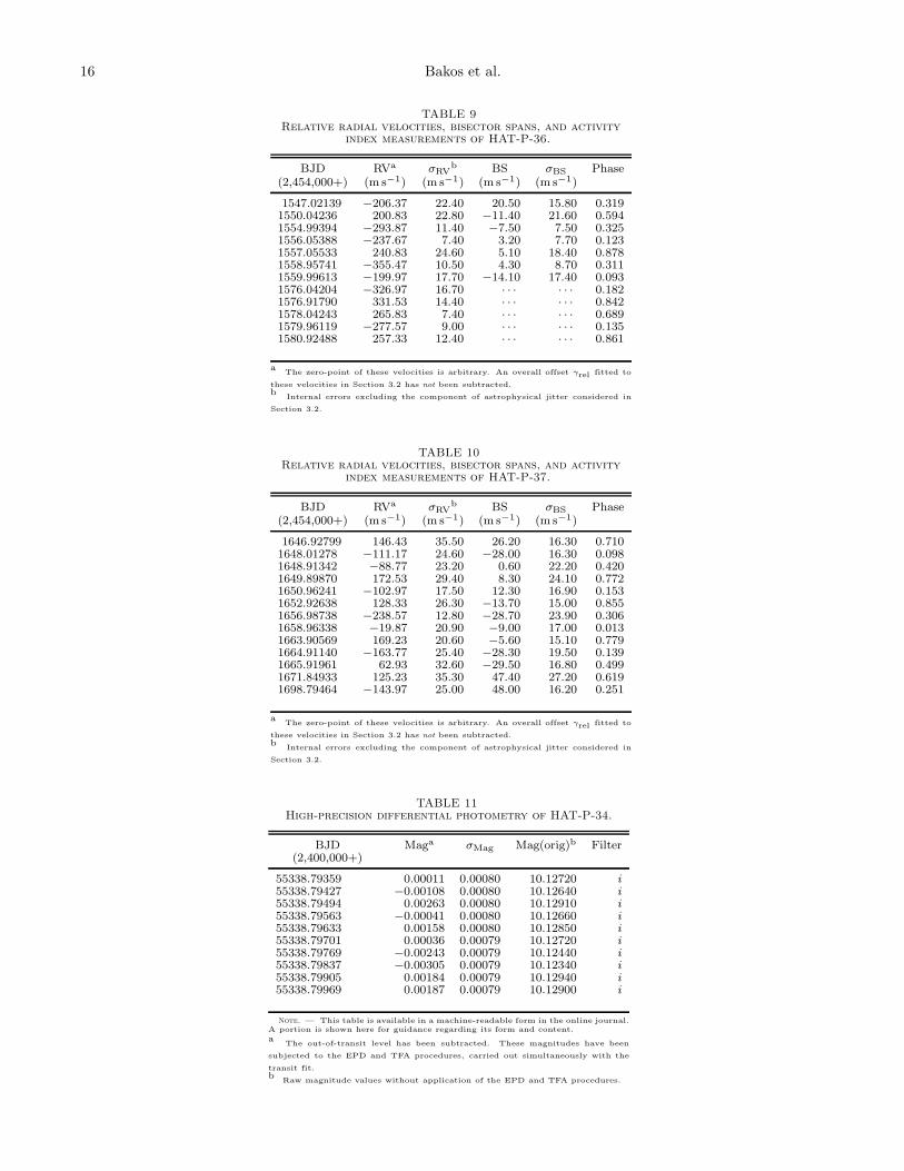
Fig. 6.— Unbinned transit light curves for HAT-P-34, acquiredwith KeplerCam at the FLWO 1.2m telescope. The light curveshave been EPD- and TFA-processed, as described in § 3.2. Thedates of the events are indicated. Curves after the first are dis-placed vertically for clarity. Our best fit from the global modelingdescribed in Section 3.2 is shown by the solid lines. Residuals fromthe fits are displayed at the bottom, in the same order as the topcurves. The error bars represent the photon and background shotnoise, plus the readout noise.

0

0.02

0.04

0.06

0.08

0.1

-0.15 -0.1 -0.05 0 0.05 0.1 0.15


∆i (

mag

)∆i

(m

ag)

∆i (

mag

)

2011 Jan 16

2011 Jan 23

2011 Mar 08

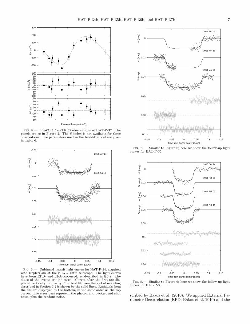
Fig. 7.— Similar to Figure 6; here we show the follow-up lightcurves for HAT-P-35.

0

0.02

0.04

0.06

0.08

0.1

0.12

0.14

-0.15 -0.1 -0.05 0 0.05 0.1 0.15


∆i (

mag

)∆i

(m

ag)

∆i (

mag

)∆i

(m

ag)

2010 Dec 24

2011 Feb 03

2011 Feb 07

2011 Feb 15


scribed by Bakos et al. (2010). We applied External Pa-rameter Decorrelation (EPD; Bakos et al. 2010) and the

8 Bakos et al.

0

0.02

0.04

0.06

0.08

0.1

0.12-0.15 -0.1 -0.05 0 0.05 0.1 0.15


∆i (

mag

)∆i

(m

ag)

∆i (

mag

)2011 Feb 23

2011 Mar 23

2011 Apr 06


Trend Filtering Algorithm (TFA; Kovacs et al. 2005) toremove trends simultaneously with the light curve mod-eling. The final time series, together with our best-fittransit light curve models, are shown in the top por-tion of Figures 6–9 for HAT-P-34 through HAT-P-37,respectively. The individual measurements, permittingindependent analysis by other researchers, are reportedin the Appendix, in Tables 11–14 (the full data are avail-able in electronic format).

3. ANALYSIS

3.1. Properties of the parent star

Stellar atmospheric parameters for HAT-P-34 andHAT-P-35 were measured using our template spectra ob-tained with the Keck/HIRES instrument, and the analy-sis package known as Spectroscopy Made Easy (SME;Valenti & Piskunov 1996), along with the atomic linedatabase of Valenti & Fischer (2005). For HAT-P-36and HAT-P-37 the stellar atmospheric parameters weredetermined by cross-correlating the TRES observationsagainst a finely sampled grid of synthetic spectra basedon Kurucz (2005) model atmospheres. This procedure,known as Stellar Parameter Classification (SPC), will bedescribed in detail in a forthcoming paper (Buchhaveet al., in preparation). We note that SPC has beenperformed in the past on numerous HATNet transitingplanet candidates (Buchhave, personal communication),and the results were consistent with those of SME.For each star, we obtained the following initial spec-

troscopic parameters and uncertainties:

• HAT-P-34 – effective temperature Teff⋆ = 6400 ±100K, metallicity [Fe/H] = +0.21± 0.1 dex, stellar

surface gravity log g⋆ = 3.98 ± 0.1 (cgs), and pro-jected rotational velocity v sin i = 24.5±1.0km s−1.

• HAT-P-35 – effective temperature Teff⋆ = 5940 ±88K, metallicity [Fe/H] = +0.01± 0.08 dex, stellarsurface gravity log g⋆ = 3.98 ± 0.1 (cgs), and pro-jected rotational velocity v sin i = 0.5± 0.5 km s−1.

• HAT-P-36 – effective temperature Teff⋆ = 5850 ±100K, metallicity [Fe/H] = +0.38± 0.1 dex, stellarsurface gravity log g⋆ = 4.73± 0.17 (cgs), and pro-jected rotational velocity v sin i = 2.86±0.5km s−1.

• HAT-P-37 – effective temperature Teff⋆ = 5570 ±100K, metallicity [Fe/H] = +0.09± 0.1 dex, stellarsurface gravity log g⋆ = 4.67 ± 0.1 (cgs), and pro-jected rotational velocity v sin i = 2.95±0.5km s−1.

Following Bakos et al. (2010), these initial valuesof Teff⋆, log g⋆, and [Fe/H] were used to determinethe quadratic limb-darkening coefficients needed in theglobal modeling of the follow-up photometry (summa-rized in Section 3.2). This analysis yields ρ⋆, the meanstellar density, which is closely related to a/R⋆, the nor-malized semimajor axis, and provides a tighter constrainton the stellar parameters than does the spectroscopicallydetermined log g⋆ (e.g. Sozzetti et al. 2007). We com-bined ρ⋆, Teff⋆, and [Fe/H] with stellar evolution modelsfrom the Yonsei-Yale (YY) series by Yi et al. (2001) todetermine probability distributions of other stellar prop-erties, including log g⋆. For each system we carried outa second SME or SPC iteration in which we adoptedthe new value of log g⋆ so determined and held it fixedin a new SME or SPC analysis, adjusting only Teff⋆,[Fe/H], and v sin i, followed by a second global modelingof the RV and light curves, together with improved limbdarkening parameters. The final atmospheric parametersthat we adopt, together with stellar parameters inferredfrom the YY models (such as the mass, radius and age)are listed in Table 5 for all four stars.The inferred location of each star in a diagram of a/R⋆

versus Teff⋆, analogous to the classical H-R diagram, isshown in Figure 10. In each case the stellar proper-ties and their 1σ and 2σ confidence ellipses are displayedagainst the backdrop of model isochrones for a range ofages, and the appropriate stellar metallicity. For compar-ison, the locations implied by the initial SME and SPCresults are also shown (in each case with a triangle).The stellar evolution modeling provides color indices

that we compared against the measured values, as a san-ity check. For each star we used the near-infrared magni-tudes from the 2MASS Catalogue (Skrutskie et al. 2006),which are given in Table 5. These were converted to thephotometric system of the models (ESO) using the trans-formations by Carpenter (2001). The resulting 2MASS-based color indices were all consistent (within 1σ) withthe stellar model based color indices.The distance for each star given in Table 5 was com-

puted from the absolute K magnitude from the modelsand the 2MASS Ks magnitudes, ignoring extinction.

3.2. Global modeling of the data

We modeled simultaneously the HATNet photome-try, the follow-up photometry, and the high-precision


4.0

5.0

6.0

7.0

8.0

9.0

10.0

11.0

12.0

13.0600065007000

a/R

*

Effective temperature [K]

HAT-P-342.0

4.0

6.0

8.0

10.0

12.0

550060006500

a/R

*


HAT-P-35

1.0

2.0

3.0

4.0

5.0

6.0500055006000

a/R

*


HAT-P-366.0

7.0

8.0

9.0

10.0

11.0

12.0500055006000

a/R

*


HAT-P-37

Fig. 10.— Comparison of the measured values of Teff⋆ and a/R⋆ for HAT-P-34 (upper left), HAT-P-35 (upper right), HAT-P-36 (lowerleft) and HAT-P-37 (lower right) to model isochrones from Yi et al. (2001). The isochrones are generated for the measured metallicity ofeach star, and for ages of 0.5Gyr and 1 to 3Gyr in steps of 0.25Gyr for HAT-P-34, and of 0.5Gyr and 1 to 14 Gyr in steps of 1Gyr forHAT-P-35, HAT-P-36 and HAT-P-37 (ages increase from left to right in each plot). The lines show the 1σ and 2σ confidence ellipses forthe measured parameters. The initial values of Teff⋆ and a/R⋆ from the initial spectroscopic and light curve analyses are represented witha triangle in each panel.

RV measurements using the procedures described byBakos et al. (2010). Namely, the best fit was determinedby a downhill simplex minimization, and was followedby a Monte-Carlo Markov Chain run to scan the param-eter space around the minimum, and establish the errorsPal (2009b). For each system we used a Mandel & Agol(2002) transit model, together with the EPD and TFAtrend-filters, to describe the follow-up light curves, aMandel & Agol (2002) transit model for the HATNetlight curve(s), and a Keplerian orbit using the formalismof Pal (2009a) for the RV curve(s). For HAT-P-34 weincluded a linear trend in the RV model, but find thatit is only significant at the ∼ 2σ level; the planet andstellar parameters are changed by less than 1σ when thetrend is not included in the fit. The parameters that weadopt for each system are listed in Table 6. In all caseswe allow the eccentricity to vary so that the uncertaintyon this parameter is propagated into the uncertaintieson the other physical parameters, such as the stellar andplanetary masses and radii; the observations of HAT-P-35b, HAT-P-36b, and HAT-P-37b are consistent withthese planets being on circular orbits.

4. DISCUSSION

We have presented the discovery of four new transitingplanets. Below we briefly discuss their properties.

4.1. HAT-P-34b

HAT-P-34b is a relatively massive Mp = 3.328 ±0.211MJ planet on a relatively long period (P =5.452654± 0.000016d), eccentric (e = 0.441± 0.032) or-bit. There are only five known transiting planets withhigher eccentricities (HAT-P-2b, e = 0.5171 ± 0.0033,Pal et al. 2010; Bakos et al. 2007a; CoRoT-10b, e =0.53±0.04, Bonomo et al. 2010; CoRoT-20b, e = 0.562±0.013, Deleuil et al. 2012; HD 17156b, e = 0.669 ±0.008, Madhusudhan & Winn 2009; and HD 80606b,e = 0.9330 ± 0.0005, Hebrard et al. 2010), all of whichhave longer orbital periods than HAT-P-34b. Of theseplanets, HAT-P-2b is most similar in orbital period toHAT-P-34b, but it has a mass that is more than twotimes larger than that of HAT-P-34b. Two planets withmasses, radii and equilibrium temperatures within 10%of the values of HAT-P-34b (assuming zero albedo andfull heat redistribution) are CoRoT-18b (Hebrard et al.2011) and WASP-32b (Maxted et al. 2010); however nei-ther of these planets has a significant eccentricity.HAT-P-34b is a promising target for measuring the

Rossiter-McLaughlin effect (Rossiter 1924; McLaughlin1924), since the host star is bright (V = 10.16), hasa significant spin (v sin i= 24.0 ± 0.5 km s−1), and thetransit is moderately long (T14 = 0.1455± 0.0016days).Also, the transit is far from equatorial (b = 0.336+0.099

−0.128),a configuration that is important for resolving the degen-eracy between v sin i and λ, which is the sky-plane pro-jected angle between the planetary orbital normal andthe stellar spin axis. Winn et al. (2010) pointed out that

10 Bakos et al.

TABLE 5Stellar parameters for HAT-P-34 through HAT-P-37

HAT-P-34 HAT-P-35 HAT-P-36 HAT-P-37

Parameter Value Value Value Value Source

Spectroscopic properties

Teff⋆ (K) . . . . . . . . . 6442 ± 88 6096 ± 88 5560 ± 100 5500± 100 Spec. Analysis.a

[Fe/H] . . . . . . . . . . . . +0.22± 0.04 +0.11± 0.08 +0.26± 0.10 +0.03± 0.10 Spec. Analysis.v sin i (km s−1) . . . 24.0± 0.5 0.5± 0.5 3.58± 0.5 3.07± 0.5 Spec. Analysis.vmac (km s−1) . . . . 5.05 4.52 0.00 . . . Spec. Analysis.vmic (km s−1) . . . . 0.85 0.85 0.00 . . . Spec. Analysis.γRV (km s−1) . . . . . −49.26 ± 0.30 40.95± 0.20 −16.29 ± 0.10 −20.53± 0.1 TRES

Photometric properties

V (mag). . . . . . . . . . 10.162± 0.073 12.46± 0.11 12.262± 0.068 13.23± 0.32 TASS,GSCb

V −IC (mag) . . . . . 0.557± 0.12 0.662± 0.12 0.760± 0.13 · · · TASSJ (mag) . . . . . . . . . . 9.460 ± 0.022 11.358± 0.024 11.046± 0.027 12.092± 0.027 2MASSH (mag) . . . . . . . . . 9.322 ± 0.030 11.072± 0.023 10.723± 0.030 11.714± 0.032 2MASSKs (mag) . . . . . . . . 9.247 ± 0.023 11.030± 0.021 10.603± 0.021 11.667± 0.020 2MASS

Derived properties

M⋆ (M⊙) . . . . . . . . 1.392 ± 0.047 1.236 ± 0.048 1.022 ± 0.049 0.929 ± 0.043 YY+a/R⋆+Spec. Analysis. c

R⋆ (R⊙) . . . . . . . . . 1.535+0.135−0.102 1.435 ± 0.084 1.096 ± 0.056 0.877+0.059

−0.044 YY+a/R⋆+Spec. Analysislog g⋆ (cgs) . . . . . . . 4.21 ± 0.06 4.21 ± 0.04 4.37± 0.04 4.52± 0.05 YY+a/R⋆+Spec. AnalysisL⋆ (L⊙) . . . . . . . . . . 3.63+0.75

−0.51 2.55+0.40−0.30 1.03± 0.15 0.62+0.11

−0.09 YY+a/R⋆+Spec. AnalysisMV (mag). . . . . . . . 3.32 ± 0.19 3.77 ± 0.15 4.83± 0.17 5.41± 0.19 YY+a/R⋆+Spec. AnalysisMK (mag,ESO) . . 2.24 ± 0.17 2.43 ± 0.13 3.14± 0.12 3.64± 0.14 YY+a/R⋆+Spec. AnalysisAge (Gyr) . . . . . . . . 1.7+0.4

−0.5 3.5+0.8−0.5 6.6+2.9

−1.8 3.6+4.1−2.2 YY+a/R⋆+Spec. Analysis

Distance (pc) . . . . . 257+22−17 535 ± 32 317 ± 17 411 ± 26 YY+a/R⋆+Spec. Analysis

a Based on the analysis of high resolution spectra. For HAT-P-34 and HAT-P-35 this corresponds to SME applied to iodine-freeKeck/HIRES spectra, while for HAT-P-36 and HAT-P-37 this corresponds to SPC applied to the TRES spectra (Section 3.1). Theseparameters also have a small dependence on the iterative analysis incorporating the isochrone search and global modeling of the data,as described in the text.b For HAT-P-34 through HAT-P-36 the value is taken from the TASS catalog, while for HAT-P-37 the value is taken from the GSCversion 2.3.2.c YY+a/R⋆+Spec. Analysis = Based on the YY isochrones (Yi et al. 2001), a/R⋆ as a luminosity indicator, and the spectroscopicanalysis results.

hot Jupiters around stars with Teff⋆ & 6250K have ahigher chance of being misaligned. Based on the effec-tive temperature of the host star 6442 ± 88K, we thusexpect that HAT-P-34b has a higher chance of misalign-ment (note that this may not necessarily yield a non-zero λ, if HAT-P-34b’s orbit is tilted along the line ofsight). Alternatively, Schlaufman (2010) used a stellarrotation model and observed v sin i values to statisticallyidentify TEP systems that may be misaligned along theline of sight, and concluded these preferentially occur atM⋆ > 1.2M⊙. Based on the stellar mass alone (1.39M⊙)we the chances for misalignment are increased.

4.2. HAT-P-35b

HAT-P-35b is a very typical Mp = 1.054 ± 0.033MJ,Rp = 1.332 ± 0.098RJ planet on a P = 3.646706 ±0.000021d orbit and with an equilibrium temperatureof Teq = 1581 ± 45K (again, assuming zero albedoand full heat redistribution). There are four otherplanets with masses, radii and equilibrium tempera-tures that are all within 10% of the values for HAT-P-35b. These are HAT-P-5b (Bakos et al. 2007b), HAT-P-6b (Noyes et al. 2008), OGLE-TR-211b (Udalski et al.2008), and WASP-26b (Smalley et al. 2010). The stellareffective temperature (6096 ± 88K) is close to the as-sumed border-line between well-aligned and misalignedsystems, making it an interesting system for testing theRM effect (with the caveat that v sin i, and thus the ex-pected amplitude of the anomaly, is low).

4.3. HAT-P-36b

HAT-P-36b is a very short period (P = 1.327347 ±0.000003d) planet with a mass ofMp = 1.832±0.099MJ,a radius of Rp = 1.264 ± 0.071RJ, and an equilibriumtemperature of Teq = 1823 ± 55K. There are two otherplanets with masses, radii, and equilibrium tempera-tures within 10% of the values for HAT-P-36b: TrES-3b(O’Donovan et al. 2007) and WASP-3b (Pollacco et al.2008).

4.4. HAT-P-37b

Like the preceding planets, HAT-P-37b also has verytypical physical properties, with Mp = 1.169± 0.103MJ,Rp = 1.178 ± 0.077RJ, P = 2.797436 ± 0.000007d,and Teq = 1271 ± 47K. Three planets with masses,radii and equilibrium temperatures within 10% of thevalues for HAT-P-37b are HD 189733b (Bouchy et al.2005), OGLE-TR-113b (Bouchy et al. 2004), and XO-5b (Burke et al. 2008). HAT-P-37 lies just outside of thefield of view of the Kepler Space mission and is listed inthe Kepler Input Catalog (KIC14) as KIC 12396036.

4.5. On the eccentricity of HAT-P-34b

According to Adams and Laughlin (2006), the eccen-tricity of a hot Jupiter’s orbit decays both due to thetides on the star and due to the tides on the planet,

14 http://www.cfa.harvard.edu/kepler/kic/kicindex.html


TABLE 6Orbital and planetary parameters for HAT-P-34b through HAT-P-37b

HAT-P-34b HAT-P-35b HAT-P-36b HAT-P-37b

Parameter Value Value Value Value

Light curve parameters

P (days) . . . . . . . . . . . . . . . . . . . . 5.452654 ± 0.000016 3.646706 ± 0.000021 1.327347 ± 0.000003 2.797436 ± 0.000007Tc (BJD) a . . . . . . . . . . . . . . . . . . 2455431.59629 ± 0.00055 2455578.66081 ± 0.00050 2455565.18144 ± 0.00020 2455642.14318 ± 0.00029T14 (days) a . . . . . . . . . . . . . . . . . 0.1455 ± 0.0016 0.1640 ± 0.0018 0.0923 ± 0.0007 0.0971 ± 0.0015T12 = T34 (days) a . . . . . . . . . . 0.0121 ± 0.0013 0.0162 ± 0.0017 0.0107 ± 0.0007 0.0153 ± 0.0013a/R⋆ . . . . . . . . . . . . . . . . . . . . . . . . 9.48± 0.64 7.45 ± 0.37 4.66± 0.22 9.32+0.42

−0.57ζ/R⋆ . . . . . . . . . . . . . . . . . . . . . . . . 14.99± 0.09 13.52 ± 0.09 24.51± 0.14 24.33 ± 0.18Rp/R⋆ . . . . . . . . . . . . . . . . . . . . . . 0.0801 ± 0.0026 0.0954 ± 0.0027 0.1186 ± 0.0012 0.1378 ± 0.0030b2 . . . . . . . . . . . . . . . . . . . . . . . . . . . 0.113+0.080

−0.062 0.128+0.078−0.066 0.097+0.057

−0.048 0.255+0.044−0.056

b ≡ a cos i/R⋆ . . . . . . . . . . . . . . . 0.336+0.099−0.128 0.357+0.092

−0.127 0.312+0.078−0.105 0.505+0.041

−0.062

i (deg) . . . . . . . . . . . . . . . . . . . . . . 87.1± 1.2 87.3 ± 1.0 86.0± 1.3 86.9+0.4−0.5

Quadratic limb-darkening coefficients b

c1, i (linear term) . . . . . . . . . . . 0.1785 0.2198 0.3142 0.3156c2, i (quadratic term) . . . . . . . . 0.3825 0.3587 0.3113 0.3032c1, z . . . . . . . . . . . . . . . . . . . . . . . . . 0.1269 · · · · · · 0.2477c2, z . . . . . . . . . . . . . . . . . . . . . . . . . 0.3728 · · · · · · 0.3082

RV parameters

K (m s−1) . . . . . . . . . . . . . . . . . . 343.1± 21.3 120.7 ± 2.2 334.7 ± 14.5 177.7± 14.8e cos ωc . . . . . . . . . . . . . . . . . . . . . 0.410 ± 0.031 −0.004 ± 0.013 −0.002± 0.032 −0.017 ± 0.039e sinωc . . . . . . . . . . . . . . . . . . . . . . 0.156± 0.052 −0.017± 0.026 0.051± 0.040 0.007 ± 0.060e . . . . . . . . . . . . . . . . . . . . . . . . . . . . 0.441± 0.032 0.025 ± 0.018 0.063± 0.032 0.058 ± 0.038ω (deg) . . . . . . . . . . . . . . . . . . . . . 20± 14 248 ± 93 95 ± 63 164 ± 84γ (m s−1 d−1) . . . . . . . . . . . . . . . 0.8683± 0.4719 · · · · · · · · ·

RV jitter

Keck/HIRES (m s−1) . . . . . . . 56.0 3.7 · · · · · ·Subaru/HDS (m s−1) . . . . . . . . 32.0 · · · · · · · · ·NOT/FIES (m s−1) . . . . . . . . . 0.0 · · · · · · · · ·FLWO 1.5/TRES (m s−1) . . . · · · · · · 33.6 25.8

Secondary eclipse parameters

Ts (BJD) . . . . . . . . . . . . . . . . . . . 2455435.721 ± 0.099 2455580.476 ± 0.030 2455565.844 ± 0.027 2455643.512 ± 0.070Ts,14 . . . . . . . . . . . . . . . . . . . . . . . . 0.1871 ± 0.0170 0.1596 ± 0.0076 0.1013 ± 0.0071 0.0981 ± 0.0083Ts,12 . . . . . . . . . . . . . . . . . . . . . . . . 0.0176 ± 0.0052 0.0156 ± 0.0019 0.0120 ± 0.0015 0.0153 ± 0.0029

Planetary parameters

Mp (MJ) . . . . . . . . . . . . . . . . . . . . 3.328± 0.211 1.054 ± 0.033 1.832± 0.099 1.169 ± 0.103Rp (RJ) . . . . . . . . . . . . . . . . . . . . . 1.197+0.128

−0.092 1.332 ± 0.098 1.264± 0.071 1.178 ± 0.077

C(Mp, Rp) d . . . . . . . . . . . . . . . . 0.23 0.49 0.11 0.02ρp (g cm−3) . . . . . . . . . . . . . . . . . 2.40± 0.63 0.55 ± 0.11 1.12± 0.19 0.89± 0.19log gp (cgs) . . . . . . . . . . . . . . . . . . 3.76± 0.08 3.17 ± 0.06 3.45± 0.05 3.32± 0.07a (AU) . . . . . . . . . . . . . . . . . . . . . . 0.0677 ± 0.0008 0.0498 ± 0.0006 0.0238 ± 0.0004 0.0379 ± 0.0006Teq (K) . . . . . . . . . . . . . . . . . . . . . 1520 ± 60 1581 ± 45 1823± 55 1271 ± 47Θe . . . . . . . . . . . . . . . . . . . . . . . . . . . 0.269± 0.029 0.064 ± 0.005 0.067± 0.005 0.081 ± 0.009〈F 〉 (109erg s−1 cm−2) f . . . . . 1.21+0.23

−0.16 1.41+0.19−0.14 2.49± 0.30 0.589+0.102

−0.075

a Tc: Reference epoch of mid transit that minimizes the correlation with the orbital period. T14: total transit duration, time between first to lastcontact; T12 = T34: ingress/egress time, time between first and second, or third and fourth contact. Barycentric Julian dates (BJD) throughoutthe paper are calculated from Coordinated Universal Time (UTC).b Values for a quadratic law, adopted from the tabulations by Claret (2004) according to the spectroscopic (SME) parameters listed in Table 5.c Lagrangian orbital parameters derived from the global modeling, and primarily determined by the RV data.d Correlation coefficient between the planetary mass Mp and radius Rp.e The Safronov number is given by Θ = 1

2(Vesc/Vorb)

2 = (a/Rp)(Mp/M⋆) (see Hansen & Barman 2007).f Incoming flux per unit surface area, averaged over the orbit.

with the tides on the planet dominating the circular-ization as long as the tidal quality factor of the planet(QP ) is not much larger than the star’s (Q⋆). Bothof these factors are highly uncertain with various the-oretical and observational constraints ranging over sev-eral orders of magnitude. In particular tidal circular-ization of main sequence stars (Claret & Cunha 1997;Meibom & Mathieu 2005; Zahn & Bouchet 1989; Zahn1989) seem to indicate 105 . Q⋆ . 106. On theother hand, the discovery of extremely short period mas-

sive planets, the two most dramatic being WASP-18b(Hellier et al. 2009) and WASP-19b (Hellier et al. 2011),seems to be inconsistent with such efficient dissipation(Penev et al. in preparation), requiring much larger val-ues Q⋆ & 108, which coincide well with the theoreti-cal values derived by Penev & Sasselov (2011), who ar-gue that binary stars and star-planet systems are sub-ject to different modes of dissipation in the star. Thetidal dissipation parameter in the planet has also been

12 Bakos et al.

the subject of many studies attempting to constrain iteither from theory (Bodenheimer, Laughlin, & Lin 2003;Ogilvie & Lin 2004) or from the observed configurationof Jupiter’s satellites (Goldreich & Soter 1966) giving105 . QP . 107.With this in mind we conclude that the circulariza-

tion of HAT-P-34b’s orbit is likely dominated by thetidal dissipation in the planet and using QP = 106 andthe expression for the tidal circularization timescale fromAdams and Laughlin (2006), we estimate the eccentricityof HAT-P-34b should decay on the scale of 2Gyr, i.e. it isnot in conflict with theoretical expectations. The possi-ble outer companion indicated by the RV trend may alsobe responsible for pumping the eccentricity of the innerplanet HAT-P-34b (see Correia et al. 2011 for a discus-sion).Figure 11 shows HAT-P-34b on the orbital period–

eccentricity plane of TEPs with well determined param-eters (using our own compilation that attempts to keepup with various refinements to these parameters). It isapparent that eccentricity is correlated with orbital pe-riod and with planet mass, as expected from tidal theory.HAT-P-34b lies in a sparse position in these diagrams;for example, it has a high eccentricity for its period, theonly similar planet being HAT-P-2b.Figure 12 is a “tidal” plot (see Fig. 3 of Pont et al.

2011), showing TEPs with well measured properties inthe a/Rp–Mp/M⋆ plane, using more data points (in-cluding the present discoveries) than Pont et al. (2011).

Since τc = (4/63)QP

√

(a3/GM⋆(a/RP )5Mp/M⋆, we ex-

pect planets with small relative semi-major axis (a/RP )or planets with small relative mass (Mp/M⋆) to be circu-larized. This is indeed the case, as shown by the intensity(color) scale representing eccentricity. For hot Jupitersthat migrate in by circularization of an initially very ec-centric orbit, the expected “parking distance” is ∼ 2aH(Ford and Rasio 2006), where aH is the semi-major axisat which the radius of the planet equals its Hill radius.The thick solid line in Figure 12 shows this relation. Afairly good match for the dividing line between the cir-cularized (denoted by black points) and eccentric (greyor color) points is at a ≈ 4aH (marked with a thin solidline). This relation now includes very small mass Keplerdiscoveries. HAT-P-34b belongs to the sparse group ofhigh relative semi-major axis (a/Rp) and massive extra-solar planets.

HATNet operations have been funded by NASA grantsNNG04GN74G, NNX08AF23G. We acknowledge partialfunding of the HATNet follow-up effort from NSF AST-1108686. We acknowledge partial support also fromthe Kepler Mission under NASA Cooperative Agree-ment NCC2-1390 (D.W.L., PI). G.K. thanks the Hun-garian Scientific Research Foundation (OTKA) for sup-port through grant K-81373. This research has made useof Keck telescope time granted through NOAO (programA289Hr) and NASA (N167Hr, N029Hr). This paper usesobservations obtained with facilities of the Las CumbresObservatory Global Telescope. Data presented in thispaper are based on observations obtained at the HATstation at the Submillimeter Array of SAO, and HATstation at the Fred Lawrence Whipple Observatory ofSAO. The authors wish to recognize and acknowledge

the very significant cultural role and reverence that thesummit of Mauna Kea has always had within the indige-nous Hawaiian community. We are most fortunate tohave the opportunity to conduct observations from thismountain.


0.1

1

10M

ass [MJ ]

0

0.2

0.4

0.6

0.8

1

1 10 100

Ecc

entr

icity

Period [d]

HAT-P-34b

Fig. 11.— Orbital-period–eccentricity diagram of TEPs with eccentricity uncertainty less than 0.1. The color (greyscale shade) of thesymbols indicates the mass of each planet. HAT-P-34b is labelled. As expected from tidal evolution theory, high eccentricity planets tendto have longer orbital periods and greater masses.

0

0.2

0.4

0.6

0.8

1

Square R

oot Eccentricity

10-5

10-4

10-3

10-2

20 100 1000

MP/M

*

a/RP

HAT-P-34b

Fig. 12.— A “tidal” diagram following Fig. 3 of Pont et al. (2011). The color (greyscale shade) of the symbols indicates the eccentricity,we assume zero eccentricity for planets that have a measured eccentricity within 4σ of zero. The dotted line shows the locus of points witha circularization time-scale of 1Gyr assuming small eccentricity, QP = 106, and P = 3d. The thick solid line shows the relation a = 2aHwhere aH is the semi-major axis at which the radius of the planet equals its Hill radius. The thin solid line shows a = 4aH .

14 Bakos et al.

REFERENCES

Adams, F. C., & Laughlin, G. 2006, ApJ, 649, 1004

Bakos, G. A., Noyes, R. W., Kovacs, G., Stanek, K. Z., Sasselov,D. D., & Domsa, I. 2004, PASP, 116, 266

Bakos, G. A., et al. 2007a, ApJ, 670, 826

Bakos, G. A., et al. 2007b, ApJ, 671, L173

Bakos, G. A., et al. 2010, ApJ, 710, 1724Bodenheimer, P., Laughlin, G., & Lin, D. N. C. 2003, ApJ, 592,

555Bonomo, A. S., et al. 2010, A&A, submittedBorucki, W. J., et al. 2011, ApJ, 736, 19Bouchy, F., Pont, F., Santos, N. C., Melo, C., Mayor, M., Queloz,

D., & Udry, S. 2004, A&A, 421, L13Bouchy, F., et al. 2005, A&A, 444, L15Buchhave, L. A., et al. 2010, ApJ, 720, 1118Burke, C. J., et al. 2008, ApJ, 686, 1331Butler, R. P. et al. 1996, PASP, 108, 500Carpenter, J. M. 2001, AJ, 121, 2851Claret, A. 2004, A&A, 428, 1001Cegla, H. M., et al. 2012, MNRAS, 421, L54Claret, A.,& Cunha, N. C. S. 1997, A&A, 318, 187Correia, A. C. M., Boue, G., & Laskar, J. 2011, ApJL in press,

arXiv:1111.5486Deleuil, M., et al. 2012, A&A, 538, A145Djupvik, A. A., & Andersen, J. 2010, in “Highlights of Spanish

Astrophysics V” eds. J. M. Diego, L. J. Goicoechea,J. I. Gonzalez-Serrano, & J. Gorgas (Springer: Berlin), p. 211

Droege, T. F., Richmond, M. W., & Sallman, M. 2006, PASP,118, 1666

Ford, E. B., & Rasio, F. A. 2006, ApJ, 638, L45Furesz, G. 2008, Ph.D. thesis, University of Szeged, HungaryGoldreich, P., & Soter, S. 1966, Icarus, 5, 375Hansen, B. M. S., & Barman, T. 2007, ApJ, 671, 861Hartman, J. D., et al. 2009, ApJ, 706, 785

Hartman, J. D., Bakos, G. A., Kipping, D. M., et al. 2011a, ApJ,728, 138

Hartman, J. D., Bakos, G. A., Torres, G., et al. 2011b, ApJ, 742,59

Hebrard, G., Desert, J.-M., Dıaz, R. F., et al. 2010, A&A, 516,A95

Hebrard, G., Evans, T. M., Alonso, R. 2011, A&A, 533, A130Hellier, C., et al. 2009, Nature, 460, 1098Hellier, C., Anderson, D. R., Collier-Cameron, A., Miller,

G. R. M., Queloz, D., Smalley, B., Southworth, J., & Triaud,A. H. M. J. 2011, ApJ, 730, L31

Howard, A. W., et al. 2010, ApJ, 721, 1467Howard, A. W., Marcy, G. W., Bryson, S. T., et al. 2011,

arXiv:1103.2541Isaacson, H., & Fischer, D. 2010, ApJ, 725, 875Johnson, J. A., Winn, J. N., Albrecht, S., Howard, A. W., Marcy,

G. W., & Gazak, J. Z. 2009, PASP, 121, 1104

Johnson, J. A., Winn, J. N., Bakos, G. A., et al. 2011, ApJ, 735,24

Kovacs, G., Zucker, S., & Mazeh, T. 2002, A&A, 391, 369

Kovacs, G., Bakos, G. A., & Noyes, R. W. 2005, MNRAS, 356,557

Kovacs, G., Bakos, G. a., Hartman, J. D., et al. 2010, ApJ, 724,866

Kurucz, R. L. 2005, Memorie della Societa Astronomica ItalianaSupplementi, 8, 14

Lasker, B. M., et al. 2008, AJ, 136, 735Latham, D. W., et al. 2009, ApJ, 704, 1107

Latham, D. W., Rowe, J. F., Quinn, S. N., et al. 2011, ApJ, 732,L24

Lissauer, J. J., Ragozzine, D., Fabrycky, D. C., et al. 2011, ApJS,197, 8

Madhusudhan, N., & Winn, J. N. 2009, ApJ, 693, 784Makarov, V. V., Beichman, C. A., Catanzarite, J. H., Fischer,

D. A., Lebreton, J., Malbet, F., & Shao, M. 2009, ApJ, 707, L73Mandel, K., & Agol, E. 2002, ApJ, 580, L171Marcy, G. W., & Butler, R. P. 1992, PASP, 104, 270Martınez-Arnaiz, R., Maldonado, J., Montes, D., Eiroa, C., &

Montesinos, B. 2010, A&A, 520, A79Maxted, P. F. L, Anderson, D. R., Collier Cameron, A., et al.

2010, PASP, 122, 1465

McLaughlin, D. B. 1924, ApJ, 60, 22Meibom, S., & Mathieu, R. D. 2005, ApJ, 620, 970Noguchi, K., et al. 2002, PASJ, 54, 855Noyes, R. W., Hartmann, L. W., Baliunas, S. L., Duncan, D. K.,

& Vaughan, A. H. 1984, ApJ, 279, 763Noyes, R. W., et al. 2008, ApJ, 673, L79O’Donovan, F. T., et al. 2007, ApJ, 663, L37Ogilvie, G. I., & Lin, D. N. C. 2004, ApJ, 610, 477Pal, A. 2009a, MNRAS, 396, 1737Pal, A. 2009b, PhD thesis, Department of Astronomy, Eotvos

Lorand University, arXiv:0906.3486Pal, A., et al. 2010, MNRAS, 401, 2665Penev, K., & Sasselov, D. 2011, ApJ, 731, 67Pollacco, D., et al. 2008, MNRAS, 385, 1576Pont, F., Husnoo, N., Mazeh, T., & Fabrycky, D. 2011, MNRAS,

414, 1278Queloz, D. et al. 2001, A&A, 379, 279Quinn, S. N., et al. 2010, ApJ, submitted, arXiv:1008.3565Rauer, H. 2011, in “Detection and Dynamics of Transiting

Exoplanets, St. Michel l’Observatoire, France”, Edited byF. Bouchy; R. Dıaz; C. Moutou; EPJ Web of Conferences,Volume 11, id.07001, 11, 7001

Rossiter, R. A. 1924, ApJ, 60, 15Saar, S. H., Hatzes, A., Cochran, W., & Paulson, D. 2003, The

Future of Cool-Star Astrophysics: 12th Cambridge Workshopon Cool Stars, Stellar Systems, and the Sun , 12, 694

Sato, B., Kambe, E., Takeda, Y., Izumiura, H., & Ando, H. 2002,PASJ, 54, 873

Sato, B., et al. 2005, ApJ, 633, 465Schlaufman, K. C. 2010, ApJ, 719, 602Schneider, J., Dedieu, C., Le Sidaner, P., Savalle, R., &

Zolotukhin, I. 2011, A&A, 532, A79Skrutskie, M. F., et al. 2006, AJ, 131, 1163Smalley, B., Anderson, D. R., Collier Cameron, A., et al. 2010,

A&A, 520, A56Sozzetti, A. et al. 2007, ApJ, 664, 1190Torres, G. et al. 2007, ApJ, 666, 121Udalski, A., et al. 2008, A&A, 482, 299Valenti, J. A., & Fischer, D. A. 2005, ApJS, 159, 141Valenti, J. A., & Piskunov, N. 1996, A&AS, 118, 595Vaughan, A. H., Preston, G. W., & Wilson, O. C. 1978, PASP,

90, 267Vogt, S. S. et al. 1994, Proc. SPIE, 2198, 362Winn, J. N., Fabrycky, D., Albrecht, S., & Johnson, J. A. 2010,

ApJ, 718, L145Wright, J. T., et al. 2011, PASP, 123, 412Yi, S. K. et al. 2001, ApJS, 136, 417Zahn, J.-P., & Bouchet, L. 1989, A&A, 223, 112Zahn, J.-P. 1989, A&A, 220, 112Wright, J. T. 2005, PASP, 117, 657

APPENDIX

SPECTROSCOPIC AND PHOTOMETRIC DATA

The following tables present the spectroscopic data (radial velocities, bisector spans, and activity index measure-ments) and high precision photometric data for the four planets presented in this paper.


TABLE 7Relative radial velocities, bisector spans, and activity index measurements

of HAT-P-34.

BJD RVa σRVb BS σBS Sc Phase Instrument

(2,454,000+) (m s−1) (m s−1) (m s−1) (m s−1)

1339.92722 −158.62 50.92 · · · · · · · · · 0.188 Subaru1339.93516 −201.37 57.36 · · · · · · · · · 0.190 Subaru1339.94290 −204.06 44.53 · · · · · · · · · 0.191 Subaru1341.11630 −246.80 47.11 · · · · · · · · · 0.406 Subaru1341.12058 −204.87 47.32 · · · · · · · · · 0.407 Subaru1341.12485 −193.24 43.00 · · · · · · · · · 0.408 Subaru1374.12069 −196.46 11.37 −2.85 6.57 0.176 0.459 Keck1374.85735 · · · · · · −9.20 4.18 0.173 0.594 Keck1374.86800 −80.49 11.89 −25.52 9.34 0.176 0.596 Keck1375.95203 285.94 10.24 −15.73 4.46 0.178 0.795 Keck1378.12823 −265.18 12.71 −13.52 7.86 0.174 0.194 Keck1379.07458 −226.26 12.73 −10.85 3.72 0.176 0.368 Keck1379.56536 −162.68 61.60 · · · · · · · · · 0.458 FIES1380.13344 −135.85 13.51 60.87 20.44 0.180 0.562 Keck1380.49378 3.45 58.70 · · · · · · · · · 0.628 FIES1381.11125 110.87 14.71 −9.04 12.64 0.175 0.741 Keck1381.55600 269.57 46.50 · · · · · · · · · 0.823 FIES1383.47949 −108.72 56.00 · · · · · · · · · 0.176 FIES1384.48968 −173.76 50.60 · · · · · · · · · 0.361 FIES1400.85414 −141.78 15.43 27.38 7.53 0.167 0.362 Keck1403.82567 497.16 15.18 38.35 6.14 0.173 0.907 Keck1404.83902 4.37 14.05 0.79 7.25 0.174 0.093 Keck1415.04513 310.06 14.03 2.76 8.29 0.168 0.965 Keck1423.66787 −115.78 78.50 · · · · · · · · · 0.546 FIES1424.64318 41.31 139.40 · · · · · · · · · 0.725 FIES1425.57489 474.54 48.70 · · · · · · · · · 0.896 FIES1426.64513 −154.35 57.60 · · · · · · · · · 0.092 FIES1464.85484 −99.38 15.03 −11.41 11.10 0.164 0.100 Keck1465.94874 −249.34 13.70 −19.33 6.92 0.163 0.300 Keck1467.71998 0.98 13.61 −12.70 8.00 0.164 0.625 Keck

Note. — Note that for the iodine-free template exposures we do not measure the RV but do measure theBS and S index. Such template exposures can be distinguished by the missing RV value.

aThe zero-point of these velocities is arbitrary. An overall offset γrel fitted to these velocities in Section 3.2

has not been subtracted.b

Internal errors excluding the component of astrophysical jitter considered in Section 3.2.c

Chromospheric activity index, calibrated to the scale of Vaughan, Preston & Wilson (1978).

TABLE 8Relative radial velocities, bisector spans, and activity index measurements

of HAT-P-35.

BJD RVa σRVb BS σBS Sc Phase Instrument

(2,454,000+) (m s−1) (m s−1) (m s−1) (m s−1)

1466.12094 −92.77 2.40 −7.06 3.64 0.129 0.139 Keck1468.11371 111.39 1.86 4.37 2.92 0.129 0.686 Keck1468.12932 · · · · · · 0.45 2.76 0.129 0.690 Keck1470.12970 −118.71 2.72 2.26 2.07 0.124 0.239 Keck1482.73469d 106.37 10.20 7.70 9.60 · · · 0.695 FIES1483.74899d 39.07 10.70 −17.40 6.50 · · · 0.973 FIES1486.74544d 97.37 8.50 8.90 8.30 · · · 0.795 FIES1488.74737d −152.93 16.90 24.70 17.20 · · · 0.344 FIES1490.72460d 78.27 8.50 −23.80 6.40 · · · 0.886 FIES1501.03468 117.01 2.39 9.98 2.63 0.127 0.713 Keck1523.09695 126.39 2.09 0.65 4.88 0.134 0.763 Keck1529.15460 −55.78 2.32 −11.07 2.00 0.129 0.424 Keck1545.14866 103.29 3.12 9.13 3.56 0.125 0.810 Keck

Note. — Note that for the iodine-free template exposures we do not measure the RV but do measure theBS and S index. Such template exposures can be distinguished by the missing RV value.

aThe zero-point of these velocities is arbitrary. An overall offset γrel fitted to these velocities in Section 3.2

has not been subtracted.b

Internal errors excluding the component of astrophysical jitter considered in Section 3.2.c

Chromospheric activity index, calibrated to the scale of Vaughan, Preston & Wilson (1978).d

The FIES/NOT observations of HAT-P-35 were not used in the analysis, see the footnote to Table 4.

Transit ingress began during the hour-long exposure obtained at phase 0.973, and the exposure obtained at

phase 0.344 has a low S/N ratio and was obtained during morning twilight.

16 Bakos et al.

TABLE 9Relative radial velocities, bisector spans, and activity

index measurements of HAT-P-36.

BJD RVa σRVb BS σBS Phase

(2,454,000+) (m s−1) (m s−1) (m s−1) (m s−1)

1547.02139 −206.37 22.40 20.50 15.80 0.3191550.04236 200.83 22.80 −11.40 21.60 0.5941554.99394 −293.87 11.40 −7.50 7.50 0.3251556.05388 −237.67 7.40 3.20 7.70 0.1231557.05533 240.83 24.60 5.10 18.40 0.8781558.95741 −355.47 10.50 4.30 8.70 0.3111559.99613 −199.97 17.70 −14.10 17.40 0.0931576.04204 −326.97 16.70 · · · · · · 0.1821576.91790 331.53 14.40 · · · · · · 0.8421578.04243 265.83 7.40 · · · · · · 0.6891579.96119 −277.57 9.00 · · · · · · 0.1351580.92488 257.33 12.40 · · · · · · 0.861

aThe zero-point of these velocities is arbitrary. An overall offset γrel fitted to

these velocities in Section 3.2 has not been subtracted.b

Internal errors excluding the component of astrophysical jitter considered in

Section 3.2.

TABLE 10Relative radial velocities, bisector spans, and activity

index measurements of HAT-P-37.

BJD RVa σRVb BS σBS Phase

(2,454,000+) (m s−1) (m s−1) (m s−1) (m s−1)

1646.92799 146.43 35.50 26.20 16.30 0.7101648.01278 −111.17 24.60 −28.00 16.30 0.0981648.91342 −88.77 23.20 0.60 22.20 0.4201649.89870 172.53 29.40 8.30 24.10 0.7721650.96241 −102.97 17.50 12.30 16.90 0.1531652.92638 128.33 26.30 −13.70 15.00 0.8551656.98738 −238.57 12.80 −28.70 23.90 0.3061658.96338 −19.87 20.90 −9.00 17.00 0.0131663.90569 169.23 20.60 −5.60 15.10 0.7791664.91140 −163.77 25.40 −28.30 19.50 0.1391665.91961 62.93 32.60 −29.50 16.80 0.4991671.84933 125.23 35.30 47.40 27.20 0.6191698.79464 −143.97 25.00 48.00 16.20 0.251

aThe zero-point of these velocities is arbitrary. An overall offset γrel fitted to

these velocities in Section 3.2 has not been subtracted.b

Internal errors excluding the component of astrophysical jitter considered in

Section 3.2.

TABLE 11High-precision differential photometry of HAT-P-34.

BJD Maga σMag Mag(orig)b Filter(2,400,000+)

55338.79359 0.00011 0.00080 10.12720 i55338.79427 −0.00108 0.00080 10.12640 i55338.79494 0.00263 0.00080 10.12910 i55338.79563 −0.00041 0.00080 10.12660 i55338.79633 0.00158 0.00080 10.12850 i55338.79701 0.00036 0.00079 10.12720 i55338.79769 −0.00243 0.00079 10.12440 i55338.79837 −0.00305 0.00079 10.12340 i55338.79905 0.00184 0.00079 10.12940 i55338.79969 0.00187 0.00079 10.12900 i

Note. — This table is available in a machine-readable form in the online journal.A portion is shown here for guidance regarding its form and content.

aThe out-of-transit level has been subtracted. These magnitudes have been

subjected to the EPD and TFA procedures, carried out simultaneously with the

transit fit.b

Raw magnitude values without application of the EPD and TFA procedures.




55578.68612 0.00996 0.00115 11.35390 i55578.68766 0.01222 0.00104 11.35670 i55578.68921 0.01205 0.00101 11.35720 i55578.69075 0.00983 0.00097 11.35550 i55578.69228 0.01193 0.00099 11.35670 i55578.69383 0.01274 0.00113 11.35760 i55578.69504 0.01155 0.00113 11.35620 i55578.69622 0.01243 0.00115 11.35790 i55578.69742 0.01049 0.00114 11.35540 i55578.69863 0.00960 0.00114 11.35430 i

Note. — This table is available in a machine-readable form in the onlinejournal. A portion is shown here for guidance regarding its form and content.



transit fit.b




55555.84870 0.00292 0.00081 10.95490 i55555.85050 0.00957 0.00083 10.96050 i55555.85205 0.00817 0.00078 10.96100 i55555.85362 0.01416 0.00079 10.96370 i55555.85516 0.01203 0.00079 10.96260 i55555.85671 0.01521 0.00079 10.96600 i55555.85826 0.01690 0.00078 10.96760 i55555.85981 0.01833 0.00079 10.96870 i55555.86135 0.01590 0.00078 10.96410 i55555.86292 0.01733 0.00078 10.96540 i




transit fit.b




55616.96855 0.02527 0.00133 12.41350 i55616.97081 0.02387 0.00135 12.41200 i55616.97308 0.02220 0.00133 12.41020 i55616.97540 0.02311 0.00131 12.41290 i55616.97774 0.02297 0.00132 12.41110 i55616.97986 0.02149 0.00133 12.40940 i55616.98176 0.02186 0.00133 12.40980 i55616.98366 0.01909 0.00131 12.40740 i55616.98555 0.02301 0.00132 12.41180 i55616.98744 0.02165 0.00129 12.40910 i




transit fit.b


Documents

Draft version October 29, 2018 arXiv:1201.0659v2 [astro-ph