Drafting and Polynomials

Many computer-generated images are defined by polynomial curves. In this module, you use polynomial functions and their corresponding graphs to study some elements of graphic design.

Masha Albrecht • Tom Teegarden

85

Drafting and Polynomials

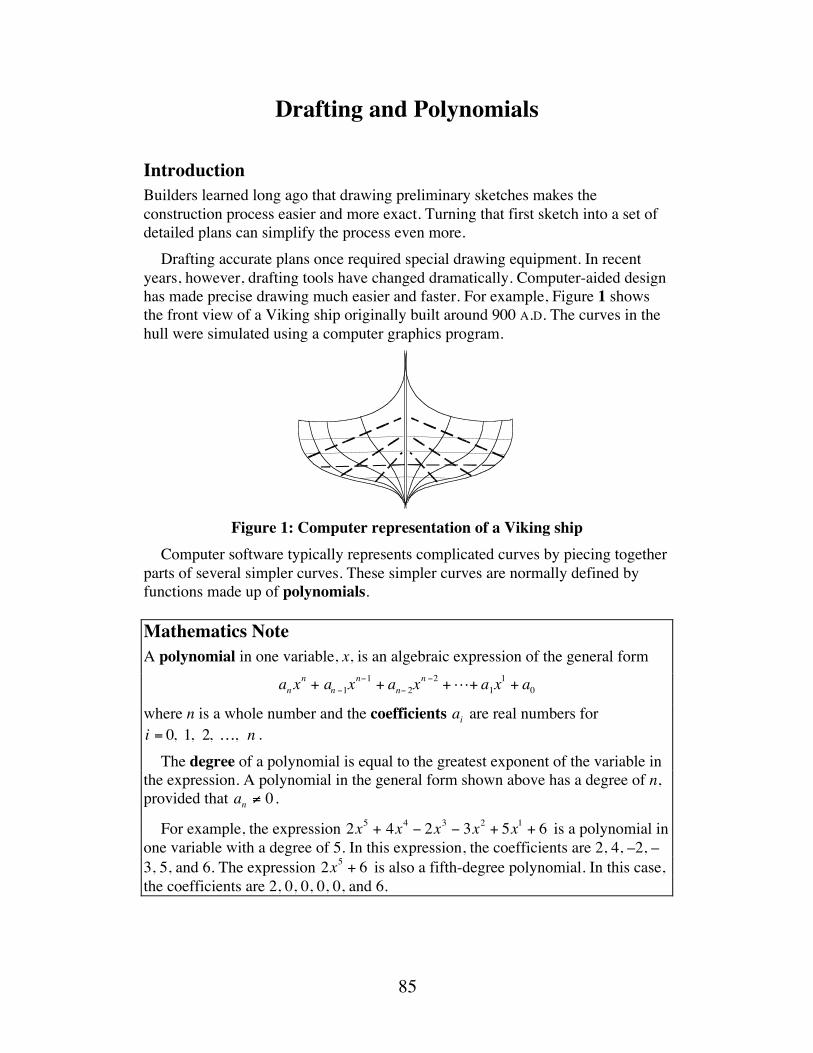
Introduction Builders learned long ago that drawing preliminary sketches makes the construction process easier and more exact. Turning that first sketch into a set of detailed plans can simplify the process even more. Drafting accurate plans once required special drawing equipment. In recent years, however, drafting tools have changed dramatically. Computer-aided design has made precise drawing much easier and faster. For example, Figure 1 shows the front view of a Viking ship originally built around 900 A.D. The curves in the hull were simulated using a computer graphics program.

Figure 1: Computer representation of a Viking ship

Computer software typically represents complicated curves by piecing together parts of several simpler curves. These simpler curves are normally defined by functions made up of polynomials.

Mathematics Note A polynomial in one variable, x, is an algebraic expression of the general form

anxn + an −1x

n−1 + an− 2xn −2 +!+ a1x

1 + a0

where n is a whole number and the coefficients ai are real numbers for i = 0, 1, 2, …, n . The degree of a polynomial is equal to the greatest exponent of the variable in the expression. A polynomial in the general form shown above has a degree of n, provided that an ≠ 0 .

For example, the expression 2x5 + 4x4 − 2x3 − 3x2 + 5x1 + 6 is a polynomial in one variable with a degree of 5. In this expression, the coefficients are 2, 4, –2, –3, 5, and 6. The expression 2x5 + 6 is also a fifth-degree polynomial. In this case, the coefficients are 2, 0, 0, 0, 0, and 6.

86

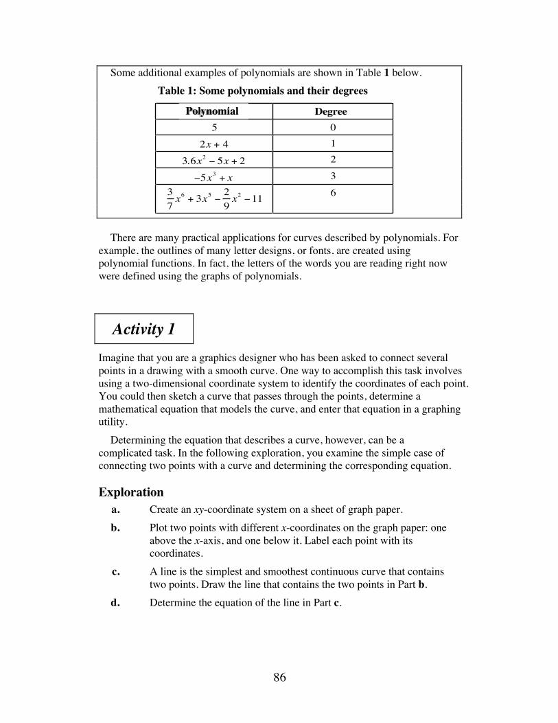
Some additional examples of polynomials are shown in Table 1 below. Table 1: Some polynomials and their degrees

There are many practical applications for curves described by polynomials. For example, the outlines of many letter designs, or fonts, are created using polynomial functions. In fact, the letters of the words you are reading right now were defined using the graphs of polynomials.

Activity 1 Imagine that you are a graphics designer who has been asked to connect several points in a drawing with a smooth curve. One way to accomplish this task involves using a two-dimensional coordinate system to identify the coordinates of each point. You could then sketch a curve that passes through the points, determine a mathematical equation that models the curve, and enter that equation in a graphing utility. Determining the equation that describes a curve, however, can be a complicated task. In the following exploration, you examine the simple case of connecting two points with a curve and determining the corresponding equation.

Exploration a. Create an xy-coordinate system on a sheet of graph paper. b. Plot two points with different x-coordinates on the graph paper: one

above the x-axis, and one below it. Label each point with its coordinates.

c. A line is the simplest and smoothest continuous curve that contains two points. Draw the line that contains the two points in Part b.

d. Determine the equation of the line in Part c.

Poynomial Degree5 0

1236

2x + 43.6x2 − 5x + 2−5x3 + x

37x6 + 3x5 − 2

9x2 −11

Polynomial

87

e. Estimate the coordinates of the point where the line intersects the x-axis. The x-coordinate of this point is the x-intercept.

This x-coordinate is also a root or zero of the function that describes the curve. It is called a zero because, when substituted for x in the function, the value of the function is 0.

Mathematics Note Factoring is the process of using the distributive property to represent a mathematical expression as a product. For example, the expression 2x + 6 can be factored into the equivalent expression 2(x +3) . Similarly, the expression 2x2 + 3x − 5 can be expressed as (2x + 5)(x −1) .

f. Using the distributive property, a linear equation in the form

y = mx + b can be rewritten as:

y = m x +bm

⎛ ⎝ ⎜ ⎞

⎠ ⎟

1. Express the equation from Part d in the form above. 2. Describe how the zero identified in Part e relates to this form of

the equation.

Discussion a. Is the graph you drew in the exploration a function? Explain your

response. b. What is the degree of a linear function? c. If for a given function g, g(7) = 0 , what does this imply about the

graph of g? d. Consider the graph of a line that intersects the x-axis at 12. What are

some possible equations for this line? e. The form of a linear equation described in Part f of the exploration,

y = m x +bm

⎛ ⎝ ⎜ ⎞

⎠ ⎟

can be rewritten by replacing m with a and b m with −c . This results in an equation of the form y = a(x − c).

1. What role does the value of a play in the graph of y = a(x − c)?

2. How is the equation of a line in the form y = a(x − c) related to its equation in slope-intercept form? Explain your response.

88

f. In this module, you will model curves by examining their zeros. What advantages are there to writing the equation of a line in the form y = a(x − c)?

Mathematics Note A function f is a polynomial function if f (x) is defined as a polynomial in x.

When the roots or zeros of a non-zero polynomial function are known, and all of these roots are real numbers, the function can be written as a product of factors, as shown below:

f (x) = a(x − c1 )(x − c2 )(x − c3 )!(x − cn )

In general, if f (c) = 0 , c is a zero of f (x) and (x − c) is a factor of f (x) .

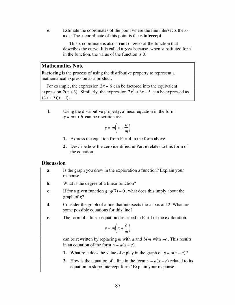
For example, Figure 2 shows a graph of f (x) = x2 + 5x − 6 . From the graph, f (−6) = 0 and f (1) = 0. Therefore, x − (−6)( ) = x + 6( ) and x −1( ) are factors of f (x) . The function can be written in factored form as f (x) = (x + 6)(x − 1).

Figure 2: Graph of a polynomial function f (x ) = x2 + 5x − 6

When a function is expressed in factored form, its zeros can be determined from the factors. For example, if g(x) = 4(x − 3)(x − 5)(x + 2) then 3, 5, and –2 are zeros of g(x) . Likewise, if h(x) = (x − 3)(x − 5)(x + 2) , then 3, 5, and –2 are its zeros.

x2 6

20

–2–6

–20

40y

f (x) = x2 + 5x − 6

89

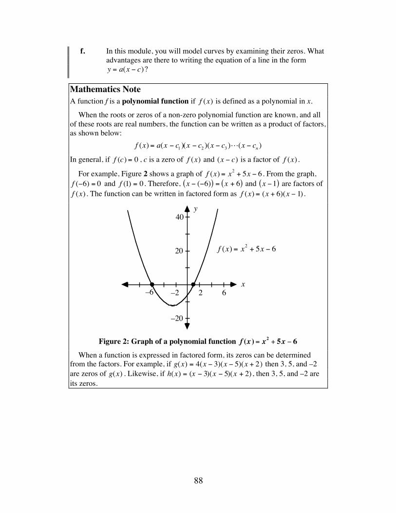
Figure 3 shows the graphs of these two functions. Notice that although the graphs of the two functions are different, their zeros are the same.

Figure 3: Graphs of two polynomial functions with same roots

Assignment 1.1 a. Using the method described in the exploration, find the equation

of a first-degree polynomial function whose graph contains the points (1,2) and (3,6). Express the equation in factored form.

b. Identify the root(s) of this polynomial function. 1.2 a. Predict the zeros for each of the following polynomial functions.

The function m(x) is said to have a double root because the factor (x − 2) appears twice.

1. f (x) = 2(x + 3)

2. h(x) = x

3. g(x) = −0.2(x − 3)(x + 2)(x − 7)

4. m(x) = (x − 2)(x − 2)

b. Create a graph of each function in Part a and estimate the zeros. c. To verify your estimates in Part b, substitute the value of each

predicted zero for x in the corresponding function. 1.3 a. Select four different real numbers. Write a polynomial function

whose roots are these numbers. b. Determine a different polynomial function with the same roots. c. Compare the graphs of the two functions in Parts a and b.

–3 x

y

–1 1 3

50

–505

g(x)

h(x)

90

1.4 a. The distributive property can be used to find the product of 8 and 16 by expressing 16 as (10 + 6) and distributing the 8 as follows:

8(10 + 6) = 80 + 48=128

Use the distributive property to multiply 3(x + 2) .

b. The product of 20 and 16 can be found by expressing 21 as (20 +1) and 16 as (10 + 6) , then using the distributive property as follows:

(20 +1)(10 + 6) = 20(10 + 6) +1(10 + 6)= (200 + 120) + (10 + 6)= 336

Use the distributive property to multiply(x + 7)(x − 4) .

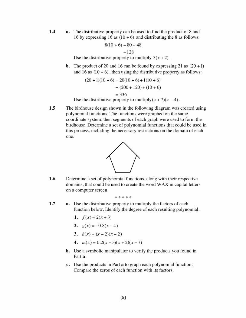
1.5 The birdhouse design shown in the following diagram was created using polynomial functions. The functions were graphed on the same coordinate system, then segments of each graph were used to form the birdhouse. Determine a set of polynomial functions that could be used in this process, including the necessary restrictions on the domain of each one.

1.6 Determine a set of polynomial functions, along with their respective

domains, that could be used to create the word WAX in capital letters on a computer screen.

* * * * * 1.7 a. Use the distributive property to multiply the factors of each

function below. Identify the degree of each resulting polynomial. 1. f (x) = 2(x + 3)

2. g(x) = −0.8(x − 4)

3. h(x) = (x − 2)(x − 2)

4. m(x) = 0.2(x − 3)(x + 2)(x − 7)

b. Use a symbolic manipulator to verify the products you found in Part a.

c. Use the products in Part a to graph each polynomial function. Compare the zeros of each function with its factors.

91

1.8 A local swimming pool is 20 m wide and 30 m long. As shown in the diagram below, the sidewalk surrounding the pool has a constant width.

a. Let w represent the width of the concrete sidewalk. Represent the

area of the sidewalk using a polynomial function in w. b. Use the distributive property to express this polynomial function

in a simplified form. * * * * * * * * * *

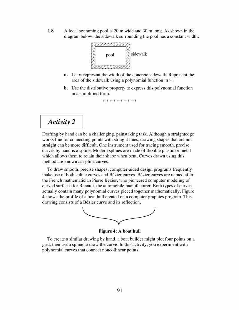
Activity 2 Drafting by hand can be a challenging, painstaking task. Although a straightedge works fine for connecting points with straight lines, drawing shapes that are not straight can be more difficult. One instrument used for tracing smooth, precise curves by hand is a spline. Modern splines are made of flexible plastic or metal which allows them to retain their shape when bent. Curves drawn using this method are known as spline curves. To draw smooth, precise shapes, computer-aided design programs frequently make use of both spline curves and Bézier curves. Bézier curves are named after the French mathematician Pierre Bézier, who pioneered computer modeling of curved surfaces for Renault, the automobile manufacturer. Both types of curves actually contain many polynomial curves pieced together mathematically. Figure 4 shows the profile of a boat hull created on a computer graphics program. This drawing consists of a Bézier curve and its reflection.

Figure 4: A boat hull

To create a similar drawing by hand, a boat builder might plot four points on a grid, then use a spline to draw the curve. In this activity, you experiment with polynomial curves that connect noncollinear points.

sidewalk pool

92

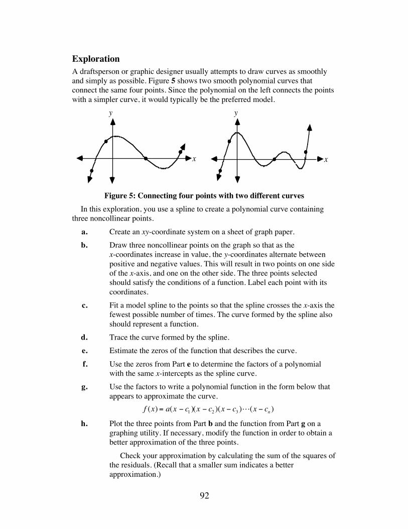
Exploration A draftsperson or graphic designer usually attempts to draw curves as smoothly and simply as possible. Figure 5 shows two smooth polynomial curves that connect the same four points. Since the polynomial on the left connects the points with a simpler curve, it would typically be the preferred model.

Figure 5: Connecting four points with two different curves In this exploration, you use a spline to create a polynomial curve containing three noncollinear points. a. Create an xy-coordinate system on a sheet of graph paper. b. Draw three noncollinear points on the graph so that as the

x-coordinates increase in value, the y-coordinates alternate between positive and negative values. This will result in two points on one side of the x-axis, and one on the other side. The three points selected should satisfy the conditions of a function. Label each point with its coordinates.

c. Fit a model spline to the points so that the spline crosses the x-axis the fewest possible number of times. The curve formed by the spline also should represent a function.

d. Trace the curve formed by the spline. e. Estimate the zeros of the function that describes the curve. f. Use the zeros from Part e to determine the factors of a polynomial

with the same x-intercepts as the spline curve. g. Use the factors to write a polynomial function in the form below that

appears to approximate the curve.

f (x) = a(x − c1 )(x − c2 )(x − c3 )!(x − cn )

h. Plot the three points from Part b and the function from Part g on a graphing utility. If necessary, modify the function in order to obtain a better approximation of the three points.

Check your approximation by calculating the sum of the squares of the residuals. (Recall that a smaller sum indicates a better approximation.)

y

x

y

x

93

Discussion a. When is it appropriate to use a line as the smoothest, simplest curve

connecting a set of points? b. What is the degree of your polynomial from the exploration? c. Is it possible to connect three points with a polynomial curve which

has a lesser degree than the one you found? Explain your response. d. How could you use the coordinates of the point of the function you

used in Part b of the Exploration to find the value of a for the function you wrote in Part g of the Exploration?

e. 1. How can you change the equation of a polynomial function without changing its zeros?

2. How do these changes affect the function’s graph?

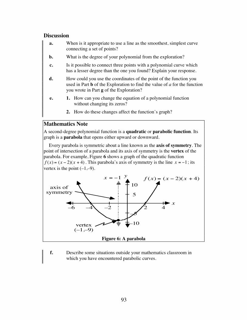
Mathematics Note A second-degree polynomial function is a quadratic or parabolic function. Its graph is a parabola that opens either upward or downward. Every parabola is symmetric about a line known as the axis of symmetry. The point of intersection of a parabola and its axis of symmetry is the vertex of the parabola. For example, Figure 6 shows a graph of the quadratic function f (x) = (x − 2)(x + 4) . This parabola’s axis of symmetry is the line x = −1 ; its vertex is the point (–1,–9).

Figure 6: A parabola

f. Describe some situations outside your mathematics classroom in

which you have encountered parabolic curves.

–4 4–2 2

vertex (–1,–9)

axis ofsymmetry

x

y

–6–5

5

10

–10

x = −1 f (x) = (x − 2)(x + 4)

94

Assignment 2.1 a. Find the coordinates of the vertex of the parabola described by the

equation y = −x(x −10) .

b. Consider a parabola that intersects the x-axis at two points. Explain how the zeros of the corresponding function can be used to find the vertex of the parabola.

c. Test your theory from Part b using another parabolic function. Describe your test and report on its outcome.

2.2 As mentioned in the introduction, the outlines of the letters in a type font can be described by polynomial functions. Although defining the different parts of a letter’s outline may require as many as 20 polynomial equations, graphic artists can easily change the size or shape of letters with the help of design software. For example, the three different G’s in the following diagram show how a letter created using Bézier curves can be altered on a drawing program.

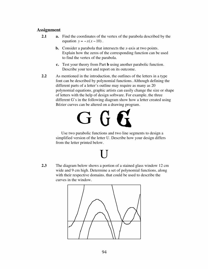
Use two parabolic functions and two line segments to design a

simplified version of the letter U. Describe how your design differs from the letter printed below.

U

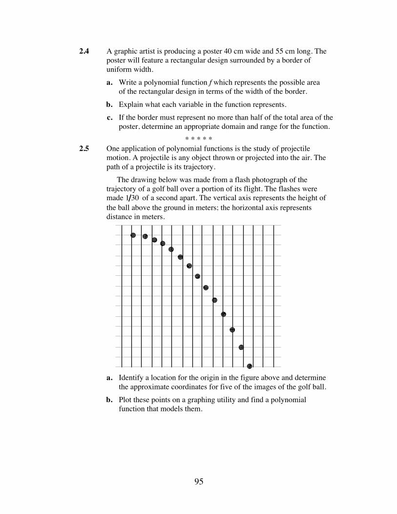
2.3 The diagram below shows a portion of a stained glass window 12 cm wide and 9 cm high. Determine a set of polynomial functions, along with their respective domains, that could be used to describe the curves in the window.

G

95

2.4 A graphic artist is producing a poster 40 cm wide and 55 cm long. The poster will feature a rectangular design surrounded by a border of uniform width.

a. Write a polynomial function f which represents the possible area of the rectangular design in terms of the width of the border.

b. Explain what each variable in the function represents. c. If the border must represent no more than half of the total area of the

poster, determine an appropriate domain and range for the function. * * * * *

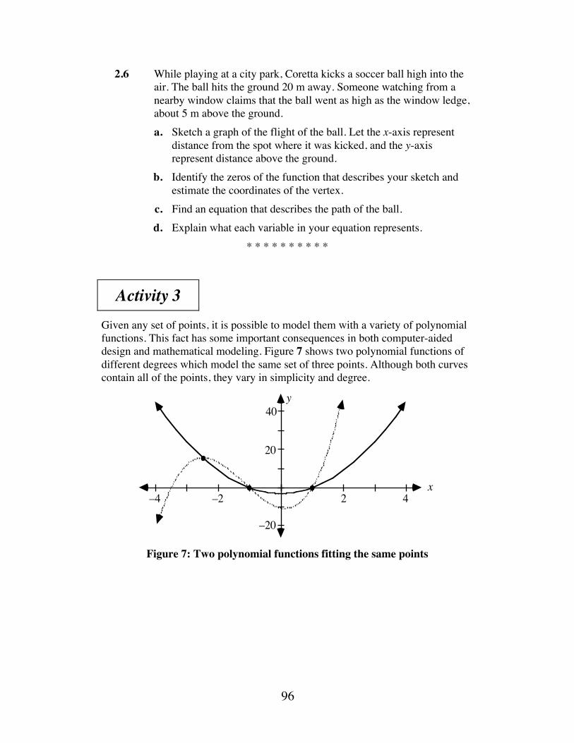
2.5 One application of polynomial functions is the study of projectile motion. A projectile is any object thrown or projected into the air. The path of a projectile is its trajectory.

The drawing below was made from a flash photograph of the trajectory of a golf ball over a portion of its flight. The flashes were made 1 30 of a second apart. The vertical axis represents the height of the ball above the ground in meters; the horizontal axis represents distance in meters.

a. Identify a location for the origin in the figure above and determine

the approximate coordinates for five of the images of the golf ball. b. Plot these points on a graphing utility and find a polynomial

function that models them.

96

2.6 While playing at a city park, Coretta kicks a soccer ball high into the air. The ball hits the ground 20 m away. Someone watching from a nearby window claims that the ball went as high as the window ledge, about 5 m above the ground.

a. Sketch a graph of the flight of the ball. Let the x-axis represent distance from the spot where it was kicked, and the y-axis represent distance above the ground.

b. Identify the zeros of the function that describes your sketch and estimate the coordinates of the vertex.

c. Find an equation that describes the path of the ball. d. Explain what each variable in your equation represents.

* * * * * * * * * *

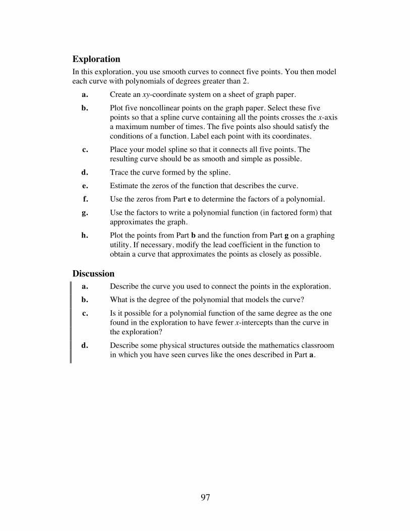
Activity 3 Given any set of points, it is possible to model them with a variety of polynomial functions. This fact has some important consequences in both computer-aided design and mathematical modeling. Figure 7 shows two polynomial functions of different degrees which model the same set of three points. Although both curves contain all of the points, they vary in simplicity and degree.

Figure 7: Two polynomial functions fitting the same points

x

y

20

40

2–2–4 4

–20

97

Exploration In this exploration, you use smooth curves to connect five points. You then model each curve with polynomials of degrees greater than 2. a. Create an xy-coordinate system on a sheet of graph paper. b. Plot five noncollinear points on the graph paper. Select these five

points so that a spline curve containing all the points crosses the x-axis a maximum number of times. The five points also should satisfy the conditions of a function. Label each point with its coordinates.

c. Place your model spline so that it connects all five points. The resulting curve should be as smooth and simple as possible.

d. Trace the curve formed by the spline. e. Estimate the zeros of the function that describes the curve. f. Use the zeros from Part e to determine the factors of a polynomial. g. Use the factors to write a polynomial function (in factored form) that

approximates the graph. h. Plot the points from Part b and the function from Part g on a graphing

utility. If necessary, modify the lead coefficient in the function to obtain a curve that approximates the points as closely as possible.

Discussion a. Describe the curve you used to connect the points in the exploration. b. What is the degree of the polynomial that models the curve? c. Is it possible for a polynomial function of the same degree as the one

found in the exploration to have fewer x-intercepts than the curve in the exploration?

d. Describe some physical structures outside the mathematics classroom in which you have seen curves like the ones described in Part a.

98

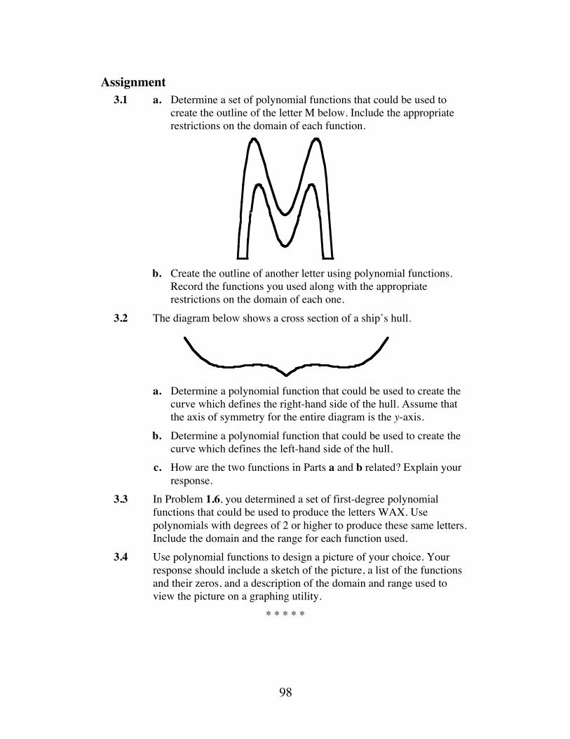
Assignment 3.1 a. Determine a set of polynomial functions that could be used to

create the outline of the letter M below. Include the appropriate restrictions on the domain of each function.

b. Create the outline of another letter using polynomial functions.

Record the functions you used along with the appropriate restrictions on the domain of each one.

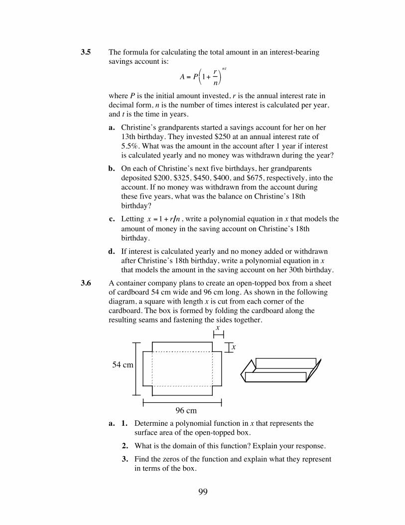
3.2 The diagram below shows a cross section of a ship’s hull.

a. Determine a polynomial function that could be used to create the

curve which defines the right-hand side of the hull. Assume that the axis of symmetry for the entire diagram is the y-axis.

b. Determine a polynomial function that could be used to create the curve which defines the left-hand side of the hull.

c. How are the two functions in Parts a and b related? Explain your response.

3.3 In Problem 1.6, you determined a set of first-degree polynomial functions that could be used to produce the letters WAX. Use polynomials with degrees of 2 or higher to produce these same letters. Include the domain and the range for each function used.

3.4 Use polynomial functions to design a picture of your choice. Your response should include a sketch of the picture, a list of the functions and their zeros, and a description of the domain and range used to view the picture on a graphing utility.

* * * * *

99

3.5 The formula for calculating the total amount in an interest-bearing savings account is:

A = P 1+rn

⎛ ⎝

⎞ ⎠

nt

where P is the initial amount invested, r is the annual interest rate in

decimal form, n is the number of times interest is calculated per year, and t is the time in years.

a. Christine’s grandparents started a savings account for her on her 13th birthday. They invested $250 at an annual interest rate of 5.5%. What was the amount in the account after 1 year if interest is calculated yearly and no money was withdrawn during the year?

b. On each of Christine’s next five birthdays, her grandparents deposited $200, $325, $450, $400, and $675, respectively, into the account. If no money was withdrawn from the account during these five years, what was the balance on Christine’s 18th birthday?

c. Letting x =1 + r n , write a polynomial equation in x that models the amount of money in the saving account on Christine’s 18th birthday.

d. If interest is calculated yearly and no money added or withdrawn after Christine’s 18th birthday, write a polynomial equation in x that models the amount in the saving account on her 30th birthday.

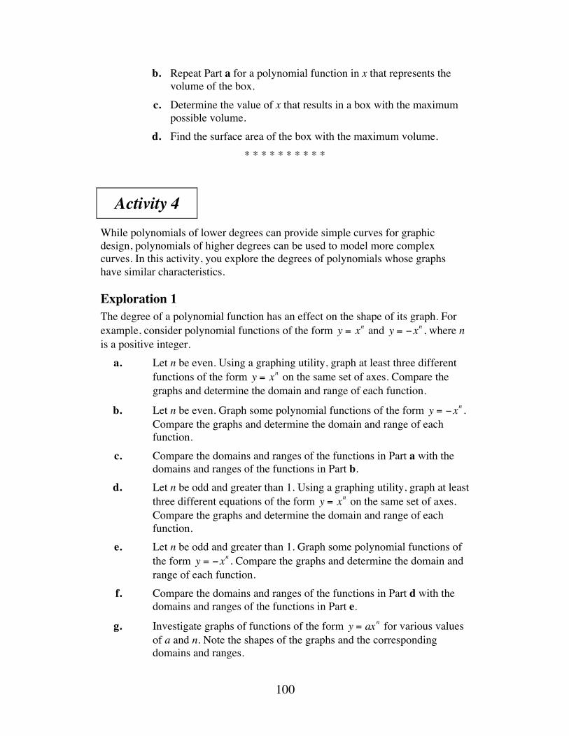
3.6 A container company plans to create an open-topped box from a sheet of cardboard 54 cm wide and 96 cm long. As shown in the following diagram, a square with length x is cut from each corner of the cardboard. The box is formed by folding the cardboard along the resulting seams and fastening the sides together.

a. 1. Determine a polynomial function in x that represents the

surface area of the open-topped box. 2. What is the domain of this function? Explain your response. 3. Find the zeros of the function and explain what they represent

in terms of the box.

x

x

54 cm

96 cm

100

b. Repeat Part a for a polynomial function in x that represents the volume of the box.

c. Determine the value of x that results in a box with the maximum possible volume.

d. Find the surface area of the box with the maximum volume. * * * * * * * * * *

Activity 4 While polynomials of lower degrees can provide simple curves for graphic design, polynomials of higher degrees can be used to model more complex curves. In this activity, you explore the degrees of polynomials whose graphs have similar characteristics.

Exploration 1 The degree of a polynomial function has an effect on the shape of its graph. For example, consider polynomial functions of the form y = xn and y = −xn , where n is a positive integer. a. Let n be even. Using a graphing utility, graph at least three different

functions of the form y = xn on the same set of axes. Compare the graphs and determine the domain and range of each function.

b. Let n be even. Graph some polynomial functions of the form y = −xn . Compare the graphs and determine the domain and range of each function.

c. Compare the domains and ranges of the functions in Part a with the domains and ranges of the functions in Part b.

d. Let n be odd and greater than 1. Using a graphing utility, graph at least three different equations of the form y = xn on the same set of axes. Compare the graphs and determine the domain and range of each function.

e. Let n be odd and greater than 1. Graph some polynomial functions of the form y = −xn . Compare the graphs and determine the domain and range of each function.

f. Compare the domains and ranges of the functions in Part d with the domains and ranges of the functions in Part e.

g. Investigate graphs of functions of the form y = axn for various values of a and n. Note the shapes of the graphs and the corresponding domains and ranges.

101

Discussion 1 a. 1. What effect does a have on the general shape of the graph of

y = axn?

2. What general statement can you make about the domain and range of the function y = axn ?

b. 1. Describe the y-values of a graph of y = xn when n is even, as x increases from –5 to 5.

2. Describe the y-values of a graph of y = xn when n is odd, as x increases from –5 to 5.

c. As the x-values of a polynomial function increase (or decrease) without bound, the change in the corresponding y-values is referred to as the end behavior of the function. What generalizations, if any, can you make about the end behaviors of the graphs in Exploration 1?

d. Is it possible for the range of a polynomial function with an even degree to contain all the real numbers? Explain your response.

e. Is it possible to predict the range of a polynomial function with an odd degree? Explain your response.

Exploration 2 Earlier in this module, you discovered a relationship between the zeros of a polynomial function and its real-number factors. In this exploration, you investigate this relationship for another group of polynomial functions of the form f (x) = anx

n + an−1xn−1 +!+ a1x

1 + a0 .

a. Using a graphing utility, graph each of the following equations on a separate coordinate system. Approximate the roots of each function.

1. f (x) = x2 − 3x + 2

2. f (x) = x3 − 6x2 +11x − 6

3. f (x) = x4 −10x3 + 35x2 − 50x + 24

4. f (x) = x5 −15x4 + 85x 3 − 225x2 + 274x −120

b. Using technology, factor each polynomial function in Part a. Do the results support the approximate roots determined from the graphs?

c. One way to translate the graph of a function involves adding a real number to its equation. Experiment with this technique by adding various real numbers to each function in Part a and graphing the results.

102

d. 1. Consider the function f (x) = x2 − 3x + 2 . Write a new function g(x) that represents a vertical translation of f (x) .

2. Graph g(x) and adjust the translation until g(x) has a different number of roots than f (x) .

3. Use the graph of g(x) to approximate its roots.

4. Use technology to factor g(x) . Do the results support the approximate roots determined from the graph?

e. Repeat Part d for each of the remaining functions listed in Part a.

Discussion 2 a. When a linear function is translated vertically, how does this

transformation affect the roots of the function? Explain your response. b. Does translating a polynomial function change its degree? c. In Parts d and e of Exploration 2, was it possible to express each

vertically translated function as a product of first-degree polynomials? How do the graphs of the vertically translated functions support your response?

d. 1. How is the number of real roots of a polynomial function of the form f (x) = a(x − c1 )(x − c2 )(x − c3 )!(x − cn ) related to its degree?

2. Is this same relationship true for all polynomial functions of the form f (x) = anx

n + an−1xn−1 +!+ a1x

1 + a0 ? Explain your response.

e. What can you tell about the degree of a polynomial by examining its graph?

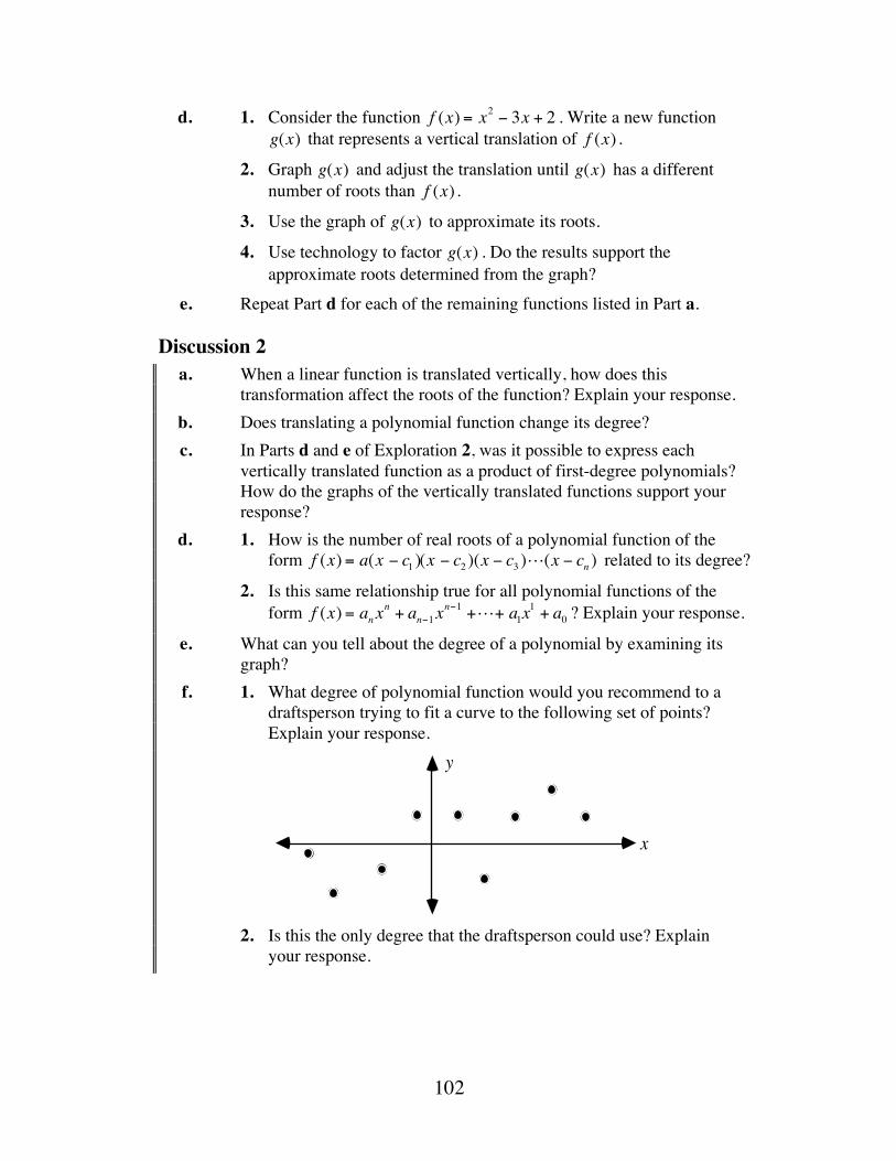
f. 1. What degree of polynomial function would you recommend to a draftsperson trying to fit a curve to the following set of points? Explain your response.

2. Is this the only degree that the draftsperson could use? Explain

your response.

x

y

103

Assignment 4.1 Examine the graphs of f (x) = (x − 2)n for n = 1, 2, 3, 4, 5, 6.

Describe any patterns you observe. 4.2 a. Determine a polynomial function with two zeros whose range is

the set of non-negative real numbers. b. Determine a polynomial function with two zeros whose range is

the set of real numbers. 4.3 a. Determine a polynomial function with a degree greater than 3 that

has exactly two distinct real roots and whose range does not include all real numbers.

b. Determine a polynomial function with a degree greater than 3 that has exactly three distinct real roots and whose range includes all real numbers.

4.4 a. Create a function whose y-values increase over a portion of the interval [–5, 5] for x and decrease over the rest of the interval.

b. Create a function whose y-values decrease as x increases from –5 to 5.

4.5 In Problem 2.2, you designed a letter U using two second-degree polynomial functions. Redesign your letter U using polynomial functions of degrees higher than 2. Compare the two designs. Do you prefer the new one or the old one? Explain your response.

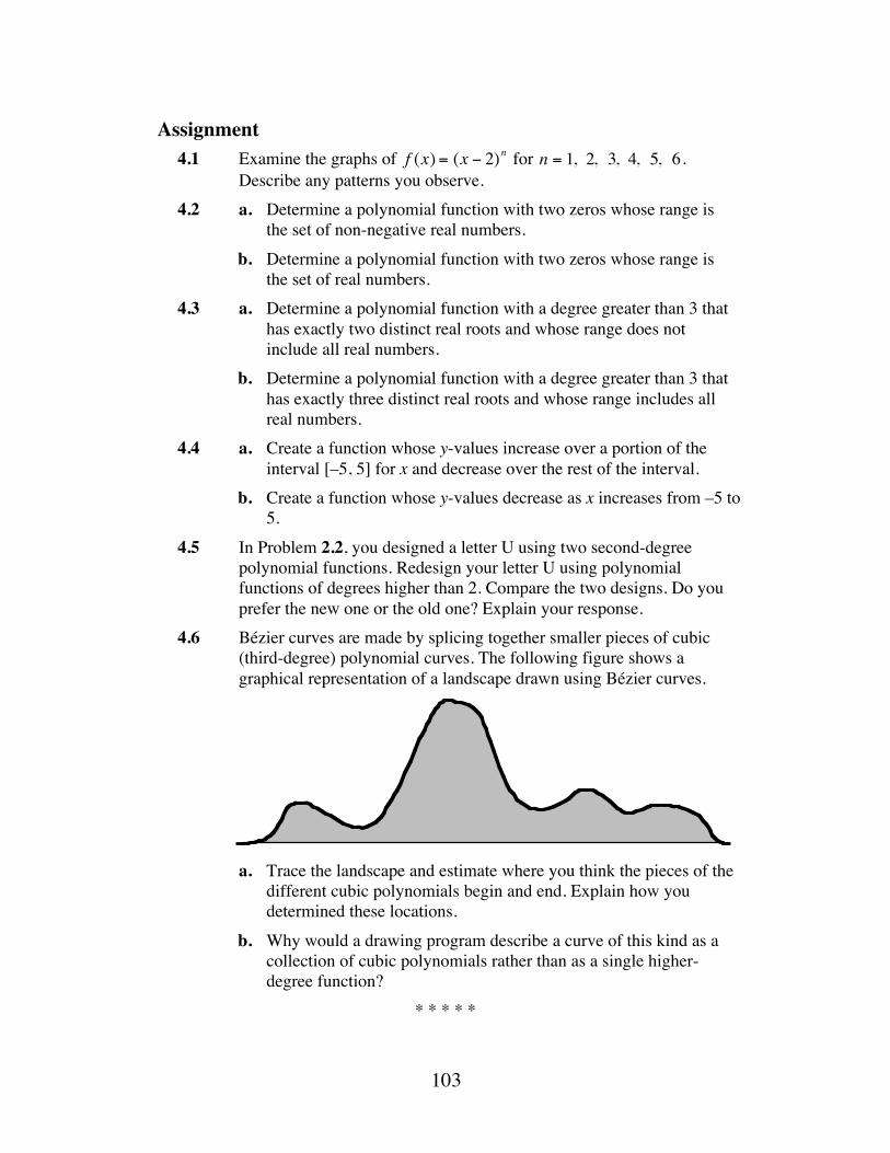
4.6 Bézier curves are made by splicing together smaller pieces of cubic (third-degree) polynomial curves. The following figure shows a graphical representation of a landscape drawn using Bézier curves.

a. Trace the landscape and estimate where you think the pieces of the

different cubic polynomials begin and end. Explain how you determined these locations.

b. Why would a drawing program describe a curve of this kind as a collection of cubic polynomials rather than as a single higher-degree function?

* * * * *

104

4.7 Consider the function f (x) = x4 − 23x2 +18x + 40 . Determine the intervals of the domain where:

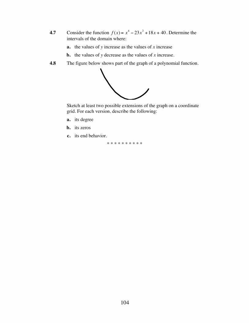
a. the values of y increase as the values of x increase b. the values of y decrease as the values of x increase. 4.8 The figure below shows part of the graph of a polynomial function.

Sketch at least two possible extensions of the graph on a coordinate

grid. For each version, describe the following: a. its degree b. its zeros c. its end behavior.

* * * * * * * * * *

105

Summary Assessment

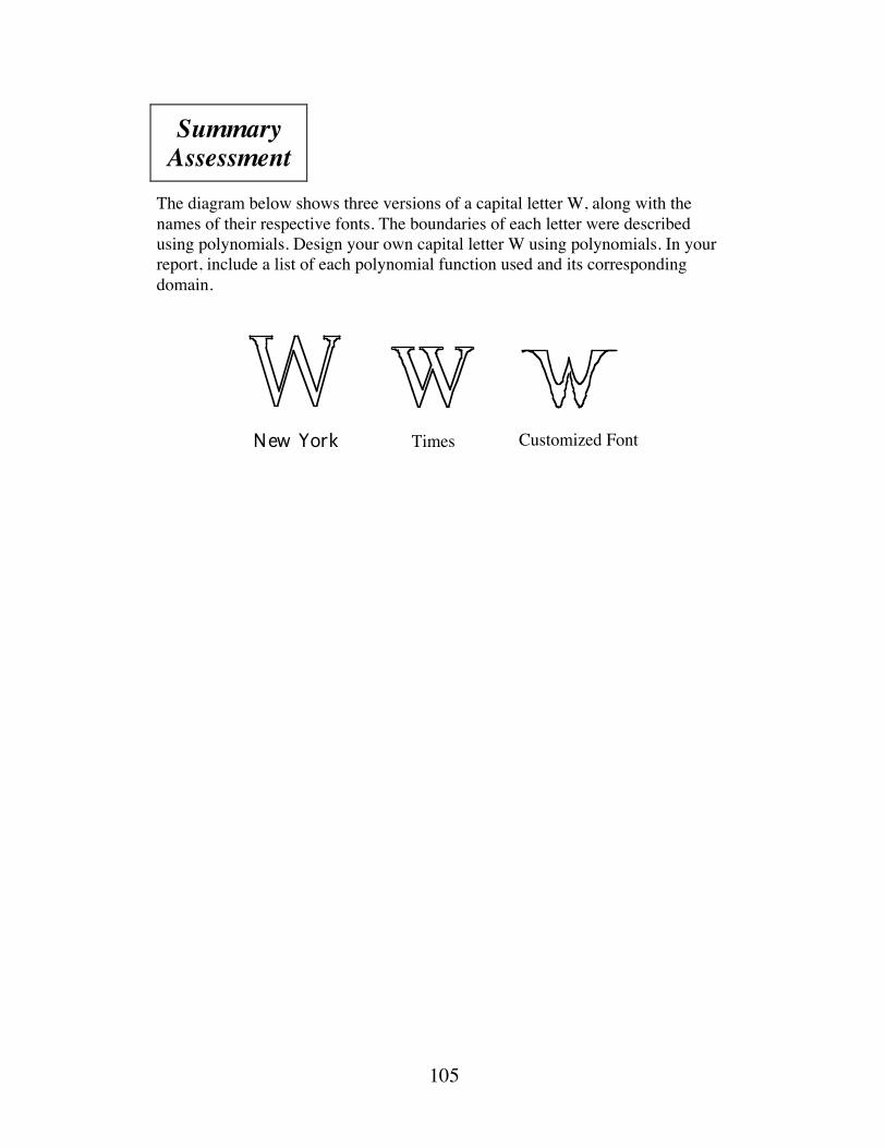
The diagram below shows three versions of a capital letter W, along with the names of their respective fonts. The boundaries of each letter were described using polynomials. Design your own capital letter W using polynomials. In your report, include a list of each polynomial function used and its corresponding domain.

New York Times Customized Font

106

Module Summary

• A polynomial in one variable, x, is an algebraic expression of the general

form

anxn + an −1x

n−1 + an− 2xn −2 +!+ a1x

1 + a0

where n is a whole number and the coefficients ai are real numbers for i = 0, 1, 2, …, n .

• The degree of a polynomial is equal to the greatest exponent of the variable in the expression. A polynomial in the general form shown above has a degree of n, provided that an ≠ 0 .

• The x-coordinate of a point where the graph of a function intersects the x-axis is an x-intercept of the function. It is also referred to as a root or zero of the function.

• A function f is a polynomial function if f (x) is defined as a polynomial in x.

• Factoring is the process of using the distributive property to represent a mathematical expression as a product.

• When the real-number roots or zeros of a polynomial function are known, the function can be written in factored form as follows:

f (x) = a(x − c1 )(x − c2 )(x − c3 )!(x − cn )

In general, if f (c) = 0 , (x − c) is a factor of f (x) .

• A second-degree polynomial function is a quadratic or parabolic function. Its graph is a parabola that opens either upward or downward.

Every parabola is symmetric about a line known as the axis of symmetry. The point of intersection of a parabola and its axis of symmetry is the vertex of the parabola.

• As the x-values of a polynomial function increase (or decrease) without bound, the change in the corresponding y-values is called the end behavior of the function.

107

Selected References Brodlie, K. W. Mathematical Methods in Computer Graphics and Design.

London: Academic Press, 1980. Gardan, Y. Mathematics and CAD. Volume 1: Numerical Methods for CAD.

Cambridge, MA: The MIT Press, 1986. Gilfillan, S. C. Inventing the Ship. Chicago: Follett Publishing Co., 1935. Lewell, John. A–Z Guide to Computer Graphics. New York: McGraw-Hill, 1985. Pokorny, C. K., and C. F. Gerald. Computer Graphics: The Principles Behind the

Art and Science. Irvine, CA: Franklin, Beedle & Associates, 1989. Special thanks to the Microsoft and Adobe companies for their assistance with this module.