DRAWDOWN PATTERNS RESULTING FROM PUMPING WELLS IN LEAKY PERCHED AQUIFERS

by

Catherine J. Goetz

Submitted in Partial Fulfillment of the Requirements for the Degree

Masters of Science in Hydrology

New Mexico Institute of Mining and Technology

Socorro, New Mexico

December 2010

ABSTRACT

This study explores the hydraulic response to pumping of leaky perched aquifers

that receive continuous recharge. We explore whether distinct drawdown curves result

that might reveal boundary effects or the position of the production well within the

aquifer. Three-dimensional saturated-unsaturated simulations were developed to generate

both circular (point-source recharge) and rectangular (line-source recharge) perched

aquifer systems. Once the simulations stabilized at quasi steady-state in response to

recharge, pumping at a constant-rate was imposed on the perched aquifer system.

Diagnostic plots of the simulated log drawdown\ log time, as well as time-derivative

curves, were analyzed. Results showed a repeatable, distinctive pattern of late-time

negative slope-derivative curves that result from the size of the perched aquifer

decreasing due to pumping and from continuing leakage through the aquitard as the

system returns to steady-state. Because leakage decreases as the size and saturated

thickness of the perched aquifer diminishes, additional water is available to meet pump

demands and the rate of drawdown in the well decreases. This behavior is due to the

small and constrained geometry of the aquifer. A lower pump rate required less reduction

in aquifer size for the system to return to equilibrium, therefore, the appearance of the

negative slope-derivative curve developed sooner than for simulations at higher pumping

rates. Surprisingly, aquifer boundary effects were not readily apparent. Specific patterns

did not emerge to indicate the well location or perched-aquifer geometry. The simulated

drawdown curves were also used to develop a methodology for obtaining transmissivity

using the Copper-Jacob straight-line analysis.

Keywords: perched aquifer; drawdown; derivative curve; low transmissivity;

MODFLOW-SURFACT; Aqtesolv.

iv

TABLE OF CONTENTS

LIST OF FIGURES ........................................................................................................... vi

LIST OF TABLES ............................................................................................................. ix

ACKNOWLEDGEMENTS .................................................................................................x

DEDICATION ................................................................................................................... xi

CHAPTER 1 - INTRODUCTION .......................................................................................1

CHAPTER 2 - CONCEPTUAL MODEL .........................................................................10

CHAPTER 3 - METHOD ..................................................................................................13

Modeling Software ....................................................................................................... 13

Verification Testing of Software .................................................................................. 15

CHAPTER 4 - NUMERICAL MODELS ..........................................................................17

Circular Perched Aquifer Model ................................................................................... 17

Rectangular Perched Aquifer Model ............................................................................ 22

CHAPTER 5 - RESULTS ..................................................................................................24

Circular Perched Aquifer .............................................................................................. 24

Model Initialization ................................................................................................... 24

Center Well Location ................................................................................................ 26

Off-Center Well Simulations .................................................................................... 34

Edge Well Simulation ............................................................................................... 37

Tight-Aquifer Simulations ............................................................................................ 39

Rectangular Model ........................................................................................................ 42

Transmissivity Estimates .............................................................................................. 44

Applicability of Time Constraints to Field Investigations ............................................ 49

CHAPTER 6 - CONCLUSIONS .......................................................................................53

REFERENCES ..................................................................................................................58

APPENDIX A - VERIFICATION OF MODELING SOFTWARE..................................64

v

APPENDIX B - ADDITIONAL MODELS ......................................................................79

vi

LIST OF FIGURES

Figure 1-1. Schematic diagram showing a perched aquifer formed on a leaky aquitard. ... 1

Figure 1-2. Schematic diagrams of aquifers and respective drawdown (black) and

derivative (red) curves: (a) unconfined with instantaneous delayed gravity drainage,

(b) leaky confined, (c) confined with impermeable boundary. Variables used: are s,

drawdown; t, time; and, d, derivative. ........................................................................ 8

Figure 2-1. Schematic diagrams illustrating (a) Circular and (b) Rectangular Aquifer

Conceptual Models. .................................................................................................. 11

Figure 4-1. Footprint of circular (a), and rectangular (b) aquifers with relative well

locations. The rectangular perched aquifer represents a section of an infinite-in-

extent stream recharge source. A- A' denotes location of the circular aquifer cross

sections presented in the following chapter. ............................................................. 21

Figure 5-1. Cross section through the center of the circular model at initial time for the

600 ft3/day pump rate test with no vertical exaggeration (a) and 5x vertical

exaggeration (b). Small arrows indicate flow direction. Shaft lengths do not

represent flow rates. .................................................................................................. 25

Figure 5-2. Cross section of the circular center well model conducted at 600 ft3/day pump

rate at 1,000 days, the test completion. Outline in background shows the initial shape

of the aquifer. ............................................................................................................ 27

Figure 5-3. Changes in drawdown (brown line), total leakage (green line), aquifer height

(blue line), and perched aquifer radius (red line) for the circular perched aquifer

model. The production well was located at the center of the perched aquifer and

pumped at a constant rate of 600 ft3/day. .................................................................. 28

Figure 5-4. Log-Log plot of drawdown (black) and derivative (red) curves within the

production well for the circular perched aquifer model. The production well was

vii

placed at the center of the perched aquifer and was pumped at a constant rate of 600

ft3/day. ....................................................................................................................... 30

Figure 5-5. Log-Log plot of drawdown (black) and derivative (red) curves within the

production well for the circular perched aquifer model for pumping rates of (a) 50,

(b) 100, and (c) 1000 ft3/day. The production well was placed at the center of the

perched aquifer. ......................................................................................................... 33

Figure 5-6. Cross section through the center of the circular perched aquifer after 1,000

days of pumping at 300 ft3/day. The well is located 50 feet outside the recharge area.

Outline in background shows the initial shape of the aquifer. .................................. 35

Figure 5-7. Log-Log plot of drawdown (black) and derivative (red) curves within the

production well for the circular perched aquifer model for pumping rates of (a) 100

and (b) 300 ft3/day. The production well was placed at 50 feet away from the edge of

the recharge area. ...................................................................................................... 36

Figure 5-8. Cross section through the center of the aquifer after 1,000 days of pumping at

40 ft3/day. The well is located 150 feet outside of the recharge area. Outline in

background shows the initial shape of the aquifer. ................................................... 38

Figure 5-9. Log-Log plot of drawdown (black) and derivative (red) curves within the

production well for the circular perched aquifer model for pumping rates of (a) 10

and (b) 40 ft3/day. The production well was placed approximately 200 feet from the

center of the aquifer. ................................................................................................. 39

Figure 5-10. Changes in drawdown (brown line), total leakage (green line), and aquifer

height (blue line) for the circular perched aquifer with low hydraulic conductivity.

The production well was located at the center of the perched aquifer and pumped at

a constant rate of 10 ft3/day. ..................................................................................... 41

Figure 5-11. Log-Log plot of drawdown (black) and derivative (red) curves within the

production well for the circular, 0.2 ft/day hydraulic conductivity, perched aquifer

model at 10 ft3/day pumping rate. The production well was in the center of the

aquifer. ...................................................................................................................... 42

Figure 5-12. Rectangular model center and edge well locations drawdown and derivative

curves for 100 ft3/day pump rate tests using an aquifer hydraulic conductivity of 3.0

ft/day. ........................................................................................................................ 44

viii

Figure 5-13. Examples of estimating the initial transmissivity value using the Cooper-

Jacob straight-line method. The semilog plots depict drawdown (black) and

derivative (red) curves from the circular aquifer, K = 3.0 ft/day, center well

locations. Upper plot is 50 ft3/day pumping rate and lower is 600 ft3/day pumping

rate. ............................................................................................................................ 47

Figure 5-14. Estimated hydraulic conductivity values for simulations presented in this

study using the Cooper-Jacob straight-line method tangent to the drawdown curve

immediately following the delayed-yield response. Values adjacent to the data point

represent the simulation pumping rate in ft3/day. The squares and circles represent

the high (3.0 ft/day) and low (0.2 ft/day) hydraulic conductivity model runs,

respectively. .............................................................................................................. 49

Figure 5-15. Log-Log drawdown and derivative curve for the constant-rate pump test

conducted in a simulated perched aquifer of hydraulic conductivity 300 ft/day

resulting in a shorter duration for the completion of the delayed-yield response and

development of the negative slope-derivative curve................................................. 51

Figure 6-1. Schematic of water sources to the well and corresponding drawdown and

derivative curve. The lag time of the delayed-yield component is not incorporated in

the water source graph. Segments A, B, C, and D represent major shifts in the well

supply and drawdown curve. .................................................................................... 54

ix

LIST OF TABLES

Table 1-1. Conversion of English to International System of Units for parameters used in

this study. .................................................................................................................... 9

Table 4-1. Circular and Rectangular Aquifer Parameters. ................................................ 19

Table 4-2. Circular and Rectangular Aquifer Pump Rates. .............................................. 22

Table 5-1. Computed and predicted transmissivity and hydraulic conductivity values for

simulations in this study. Abbreviations: C is circular; R is rectangular; Tex is

texture; S is sand; Loc. is Location; Cent is center; Predict is predicted; T is

transmissivity; b is aquifer thickness; K is hydraulic conductivity; Simul is

simulation. ................................................................................................................. 48

x

ACKNOWLEDGEMENTS

I am grateful to my committee members Mike Fort, Dr. Mark Person (advisor),

and Dr. Fred Phillips whose insights and suggestions furthered my education through the

successful completion of this study. I wish to extend a special thanks to Mike Fort, who

as an alumnus of Tech donated many hours of his time and expertise. Finally I wish to

thank Dr. John Wilson who provided the genesis of this project.

xi

DEDICATION

Although a small token, this thesis is dedicated to my husband Miles Diller.

Returning to school, I left my career that I enjoyed as a geologist, moved to Socorro and

commuted home on the weekends just because I was curious about hydrogeology. I have

good reason to ask myself "what was I thinking?" I do not know. But I do know that

through all this, Miles has been supportive and is deserving of more than a dedication in a

thesis that sits on a library shelf collecting dust.

xii

This thesis is accepted on behalf of the

Faculty of the Institute by the following committee:

____________________________________________________________________

Advisor

____________________________________________________________________

____________________________________________________________________

____________________________________________________________________

Date

I release this document to the New Mexico Institute of Mining and Technology.

Student's Signature Date

1

CHAPTER 1 - INTRODUCTION

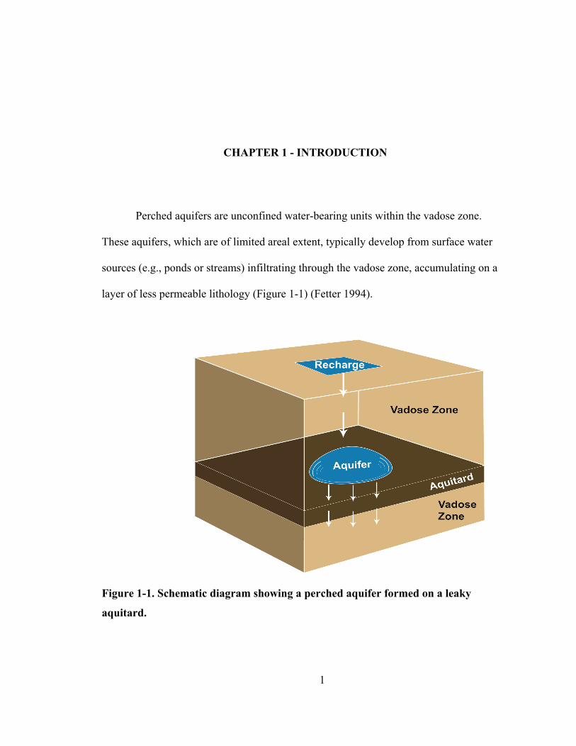
Perched aquifers are unconfined water-bearing units within the vadose zone.

These aquifers, which are of limited areal extent, typically develop from surface water

sources (e.g., ponds or streams) infiltrating through the vadose zone, accumulating on a

layer of less permeable lithology (Figure 1-1) (Fetter 1994).

Figure 1-1. Schematic diagram showing a perched aquifer formed on a leaky

aquitard.

2

Perched aquifers are of little importance for municipal water supply but may

contribute to contaminant transport, particularly if the recharge source is an industrial

discharge pond or stream receiving untreated effluents (Hueni 2010). Investigation of

potentially contaminated sites often involves the drilling, installation, and subsequent

testing of monitoring wells to determine the aquifer transmissivity and storage parameters

(Hall 1996). These properties can be obtained using single-well aquifer test methods

(Driscoll 1986). During these tests the well drawdown is measured over time while pump

discharge is maintained constant. The resulting drawdown curve is evaluated using

analytical solutions and their associated graphical depictions to estimate the aquifer

parameters (Schwartz et al. 2003). These solutions assume an unconfined aquifer of

infinite radial extent, ignoring the boundary effects of the perched system. If a constant-

rate pump test could also determine properties unique to a perched aquifer (e.g., distance

to a perched aquifer boundary) this would be of benefit to remediation strategies.

Previous perched-aquifer research has largely focused on the role of these water-

bearing units as a component of local or regional groundwater investigations. The

application of these studies is varied, reflecting the participation of perched aquifers in

diverse aspects of groundwater functions. Rains et al. (2006) showed the relationship of

perched aquifers to certain wetland ecosystems by evaluating the connectivity of perched

systems to vernal pools. Wu et al. (1999) investigated the effect of perched aquifers in

construction and waste applications by exploring their occurrence and lateral

groundwater flow at a proposed subsurface waste repository. Other studies investigated

the role of perched aquifers as a groundwater migration pathway for potential

contaminants. These investigations typically focused on the presence or absence of

3

contaminants in perched units and the connectivity of these units within the local or

regional groundwater system. A range of contaminants occurring in perched aquifers

have been examined including sea water, petroleum contaminants, pesticides, etc.

(Reichard et al. 1995, Cozzarelli et al. 1999, Behaera et al. 2003).

Mathematical descriptions have been generated for perched aquifers serving as

subsurface water storage reservoirs. Bouwer et al. (1999) presented a solution for

predicting the height of a perched aquifer subjected to artificial recharge, while Anakhaev

(2009) examined a similar subsurface feature by obtaining a steady-state flow solution for

a perched mound. Previous research has also explored the formation of perched aquifers

given certain structural features. Bagtzoglou (2003) investigated the mechanisms for the

genesis of perched water in fault systems and the recharge rates required to sustain the

system.

While there are numerous studies on perched aquifers as a component of local or

regional groundwater systems, analytical solutions describing the behavior of a perched

aquifer are few in number with little analysis on the hydraulic response of a perched

aquifer to perturbations. Therefore, conventional analysis of constant-rate pump tests

conducted on perched systems is chiefly based on solutions formulated for infinite-in-

extent unconfined aquifers. These solutions include the delayed-yield solution first

developed by Boulton (1954) and expanded upon by numerous researchers (e.g. Neuman

1972, 1974; Moench 1995). The analytical solutions may provide insights into aspects of

the unconfined behavior of perched aquifers. However, they do not address several

important attributes of perched aquifers including their limited spatial extent and variable

thickness.

4

Mathematical advances in describing the perched aquifer response to

perturbations is largely a product of unconfined flow studies having components relevant

to perched systems. For example, Serrano (2003) presents a model for groundwater flow

experiencing a nonlinear moving boundary with vertical flow that was field-verified on a

perched aquifer with periodic recharge. Although the development of analytical solutions

and numerical models representing the nonlinear behavior associated with perched

aquifers (vertical flow, moving phreatic surface of variable thickness) presents

challenges, it has been suggested that the lack of literature in this area likely reflects a

focus on groundwater supply development thereby leaving perched aquifer hydrology "an

unexplored frontier" (Fogg 2003).

This study is perhaps the first to explore the hydrologic response of a leaky

perched aquifer to constant pumping. The goal is to ascertain whether distinctive

drawdown curves result that could enable the unit's limited extent and geometry to be

defined, as well as the position of the well within the aquifer. To achieve this, three-

dimensional simulations using MODFLOW-SURFACT (HydroGeoLogic, Inc. 2007)

were developed to generate perched aquifers and subsequently perform the constant-rate

pump tests. The pump test results were analyzed using Aqtesolv (Duffield 2007) to

generate drawdown and time-derivative curves for aquifer behavior analysis. The time-

derivative curve is calculated as the derivative of drawdown with respect to the natural

logarithm of time and will be referred to as the derivative curve in this study.

As the drawdown pattern from a constant-rate pump test conducted on a leaky

perched aquifer was unknown, an initial review of existing analytical solutions was

instructive. The Theis solution (1935) for a confined aquifer of infinite lateral extent

5

serves as a guide to ideal confined aquifer behavior, while additional analytical solutions

describe particular components of the leaky perched-aquifer system. Specifically, the

drawdown and derivative curves from the leaky perched aquifer were compared to

analytical solutions of the flow equations for three sets of aquifer boundary conditions:

unconfined aquifer with instantaneous delayed yield, leaky aquitard, and no-flow lateral

boundary (Figure 1-2). We hypothesized that drawdown patterns from an aquifer test

conducted in a leaky perched aquifer could exhibit some or all of these features. Neuman

(1972) solved the flow equation for a laterally infinite unconfined aquifer with

instantaneous delayed gravity drainage, also referred to as delayed yield. The time-

drawdown curve produces an “S” shape reflecting the early time response to elastic

storage, intermediate time contribution from delayed gravity drainage of water from the

pores within the cone of depression, and late time radial flow of the infinite-acting

aquifer (Figure 1-2 a). (Schwartz et al. 2003). The derivative curve identifies the delayed

yield by a "V" shape while the late time, infinite-acting radial flow is a horizontal line

(Renard et al. 2009). Figure 1-2 (a) presents an example of the drawdown and derivative

curves depicting the pattern that results from delayed yield in an infinite aquifer. A

schematic of this idealized aquifer scenario is also shown.

A second component of time-drawdown response to pumping that may be found

in the perched-aquifer scenario is the effect of a leaky aquitard (Figure 1-2 b). The

analytical solution for pumping of a confined aquifer with an overlying leaky aquitard

and unconfined aquifer was developed by Hantush and Jacob (1955). Leakage across a

semi-permeable confining unit provides an additional supply of water to the confined

aquifer, resulting in less drawdown at late time than would be predicted from the Theis

6

solution (Figure 1-2 b). The derivative curve reflects this; the rate of drawdown in the

well decreases at intermediate time and the slope of the derivative becomes negative,

dropping to zero when the drawdown stabilizes at late time (Figure 1-2 b). For a perched

aquifer, the leakage is downward out of the aquifer, diminishing as the head declines due

to pumping.

A third hydrologic response considered in this study is the impact due to

boundaries (in our case, the edge of the perched aquifer). Image well theory is often

utilized to determine drawdown response to boundaries by mimicking a physical barrier

using superposition theory. The effects of an imaginary or "image well" are added to the

predicted drawdown from the "real" well. Where the cone of depressions of the real and

image wells overlap, the drawdowns are added (Ferris et al. 1962). Encountering an

impermeable boundary has the effect of increasing (doubling) the drawdown predicted by

the Theis solution at the boundary. Figure 1-2(c) depicts the increase in slope in the

drawdown and derivative curves in a confined aquifer pump test when an infinite linear

impermeable boundary is encountered (Renard et al. 2009). A perched aquifer is bounded

by the locus of positions at which the saturated thickness goes to zero. While application

of the method of images to unconfined aquifers with variable saturated thickness is not

strictly applicable, analogous results of positive slope drawdown and derivative curves

were observed in verification tests on unconfined aquifers of uniform thickness where

drawdown encountered model no-flow boundaries (Appendix A) (Schwartz et al. 2003).

Additional techniques in reservoir test analysis use diagnostic plots and tools to describe

flow systems deviating from infinite-in-extent models (Bourdet et al. 1989, Cinco-Ley et

al. 1981, Barker 1988). The methods describe flow regimes having limited boundaries

7

that also depict diagnostic derivative plots of increasing slopes. While these are typically

applied to fracture-flow analysis in the petroleum industry, application of these

techniques to hydrogeological problems is valid and appropriate (Walker et al. 2003,

Renard et al. 2009). The drawdown curve response to these three cases of aquifer

behavior - unconfined with instantaneous delayed yield, leaky, and boundaries - serve to

facilitate evaluations of the simulated constant-rate pump tests of the leaky perched

aquifer by either presence or absence and sequence of these features in test results. Using

these identified patterns as well as unanticipated responses, the drawdown and derivative

curves were analyzed to determine if constant-rate pump tests could be used to identify a

perched aquifer as limited in extent, or to identify it as of a particular geometry, or to

determine the well position within the perched aquifer.

8

Figure 1-2. Schematic diagrams of aquifers and respective drawdown (black) and

derivative (red) curves: (a) unconfined with instantaneous delayed gravity drainage,

(b) leaky confined, (c) confined with impermeable boundary. Variables used: are s,

drawdown; t, time; and, d, derivative.

In the remainder of this manuscript, we describe the perched aquifer conceptual

models used in this study (Chapter 2). The methods and software used, including the

governing equation used in MODFLOW-SURFACT, are described in Chapter 3 with the

9

numerical grids constructed for the pond and stream based recharge scenarios following

in Chapter 4. We then present simulation results (Chapter 5) followed by the discussion

of findings and concluding remarks (Chapter 6). Appendix A contains the results of

software verification testing and Appendix B presents additional models of infinite-in-

extent unconfined aquifers to assist in the perched aquifer drawdown curve analyses.

The simulations were conducted in the United States Customary System or

English measurement units. The use of the English system facilitated refined

discretization conducted on test models. The following table (Table 1-1) provides

conversion to many common values used in this study.

Parameter English International System of Units

Length 1 foot (ft) 0.3048 meters (m)

Area 1 square foot (ft2) 0.0929 square meters (m2)

Volume 1 cubic foot (ft3) 0.0283 cubic meter (m3)

Hydraulic Conductivity 1 foot/day (ft/day) 3.528E-6 meter/second (m/s)

Transmissivity 1 square foot/day (ft2/day) 1.075E-6 square meters/second (m2/s)

Flow Rate 1 cubic foot/day (ft3/day) 3.277E-7 cubic meter/second (m3/s)

Table 1-1. Conversion of English to International System of Units for parameters

used in this study.

10

CHAPTER 2 - CONCEPTUAL MODEL

Our conceptual model of a perched aquifer system used in this study consists of a

thick vadose zone bounded at the base by a less permeable, leaky aquitard of continuous

lateral extent and finite thickness. Below the base of the aquitard was a thick unsaturated

layer having the same properties as the upper vadose zone. All hydrostratigraphic units

were modeled as isotropic and homogenous. Recharge was applied over a portion of the

top surface, infiltrating through the vadose zone and accumulating on the top of the

aquitard to form a perched aquifer. This zone of enhanced recharge could represent

surface water sources such as a pond, stream, or impoundment. Quasi steady-state

conditions for the perched aquifer were assumed. We required that the total recharge

entering the system equaled the total volume of water leaking through the aquitard. Note

that the footprint of the perched aquifer was less than the lateral extent of the aquitard.

Two perched aquifer shapes were examined. First, a circular aquifer resulting from a

small square recharge area was considered. This recharge geometry is intended to

replicate discharge from a pond or impoundment. Second, a rectangular aquifer formed

by a thin rectangular recharge area extending across the model was examined. This

recharge geometry is intended to represent infiltration from a stream or river (Figure 2-1).

11

Figure 2-1. Schematic diagrams illustrating (a) Circular and (b) Rectangular

Aquifer Conceptual Models.

Following perched-aquifer development for these two scenarios, a constant-rate

pump test was conducted using a fully penetrating extraction well. Once extraction

began, the system shifted from steady-state to transient conditions. To replicate field

operations where observation wells may be lacking, drawdown data was collected from

the extraction well. The extraction well was placed in differing locations within each

a

b

12

aquifer shape to assess the effect of well placement on drawdown curves. The circular

aquifer was evaluated in three locations: center, off-center, and edge. The rectangular

aquifer was examined in two locations: center and edge. In addition to various well

placements, each shape was assessed using two differing aquifer hydraulic conductivities

(K), 0.2 ft/day and 3.0 ft/day. Recharge rates required pairing to appropriate hydraulic

conductivities of the aquifer (K) with those of the aquitard (K') so as to produce a

sufficient saturated thickness to enable a pump test to be conducted and also to prevent

the lateral spreading of the growing aquifer from encountering the boundaries of the

modeled flow domain before steady-state conditions were reached. The lower hydraulic

conductivity (0.2 ft/day) supported perched-aquifer growth at a low recharge rate (5.5E-3

ft3/day) over a relatively long duration (approximately 550 years), intended to be

comparable to typical natural conditions, while the higher hydraulic conductivity required

an intense (0.25 ft3/day), short-duration (approximately 5.5 years) recharge event that

could simulate anthropogenic releases.

13

CHAPTER 3 - METHOD

Modeling Software

Because multiple processes (leakage, delayed yield, boundary effects) can all

interact simultaneously while pumping a perched aquifer, we utilized numerical modeling

in this study. The governing equation describing saturated-unsaturated flow through the

vadose zone used in this study is given by:

t

hSS

t

SW

z

hkK

zy

hkK

yx

hkK

x sww

rwzzrwyyrwxx ∂∂

∂∂

φ∂∂

∂∂

∂∂

∂∂

∂∂

∂∂ +=−

+

+

(1)

Where xxK , yyK , zzK is saturated hydraulic conductivity in the principal directions

(ft/day), k is relative permeability (unitless), h is hydraulic head (ft), W is sources or

sinks (ft3/day), ϕ is drainable porosity or specific yield (Sy) (unitless), S is degree of

saturation (unitless), and S is specific storage (1/ft) (HydroGeoLogic, Inc. 2007).

This equation was solved numerically using the block-centered finite-difference

groundwater flow-modeling package MODFLOW-SURFACT. MODFLOW-SURFACT

is a commercial software package developed by HydroGeoLogic, Inc. (2007), with the

pre- and post-processor Visual MODFLOW (Schlumberger 2009). Input data formats for

MODFLOW-SURFACT are based on the commonly used saturated zone finite-

difference method groundwater model named the United States Geological Survey

(USGS) Modular Flow Model (MODFLOW) (McDonald and Harbaugh 1988).

14

MODFLOW-SURFACT provides additional capabilities to MODFLOW for

unsaturated/saturated interactions and replication of well pumping which include the

ability to simulate the vertical unsaturated/saturated sequences seen in perched aquifers,

the use of well packages which permit the addition of wellbore storage and the

apportioning of well withdrawal to well nodes, and a simplified approach (linearization)

to the analysis of variably-saturated flow. This simplification utilizes pseudo-soil to

define the relationship between pressure head and relative permeability and saturation to

assess unconfined flow in lieu of soil type functions (e.g., van Genuchten functions)

(HydroGeoLogic, Inc. 2007). Saturated/unsaturated flow is mathematically highly

nonlinear. MODFLOW-SURFACT linearizes the degree of saturation, Sw, and thus

relative permeability, krw, in order to achieve high computational efficiency and mass

conservation. The degree of saturation, which is a function of pressure head (ψ), is

determined for a grid cell by assigning a value of 1 for cells with the hydraulic head

above or at the elevation of the top of the cell and zero when the head is at or below the

bottom elevation of the grid cell. Integrating vertically across the grid cell provides a

straight line relationship, Sw (ψ) = wS . The dimensionless value for wS ranges between 0

and 1. Relative permeability, krw, depends on the degree of saturation of the cell.

Therefore, setting krw = wS further reduces the complexity of the nonlinear variably

saturated flow equation (Panday et al. 2008). While these functional relationships lack the

specificity of soil type functions, they provided a computationally efficient means to

assess the variably saturated flow.

After completing the pump-test simulations, drawdown data was exported from

MODFLOW-SURFACT and imported into Aqtesolv (Duffield 2007). Two graphical

15

depictions of the aquifer test were generated for each simulation: the drawdown curve,

representing either the log or linear drawdown versus log time, and the time-derivative

curve. The time-derivative of the drawdown is referred to as the derivative curve in this

study and as is computed by:

[ ])ln()ln(

)ln()ln(

)ln()ln(

)ln( 21

12

22

1

1

tt

tt

st

t

s

itd

ds

Δ+Δ

Δ

ΔΔ+Δ

ΔΔ

= (2)

Where i is the point of interest on the drawdown curve, s is drawdown, and t is

time (Duffield 2007). The method was presented by Bourdet et al. (1989) as a preferred

approach to calculating the derivative due to its accuracy over the duration of the test.

Noise reduction in the derivative curve is implemented using the Bourdet method where

the distance between the points of interest is determined by a variable, L, that specifies

the separation between the points of interest according to the fraction of log cycle. Values

of L generally range from 0.1 to 0.5 log cycles, where 0.5 would be considered in severe

cases (Bourdet et al. 1989). Figures of the drawdown and derivative curves presented in

this study were generated using Aqtesolv.

Verification Testing of Software

The MODFLOW-SURFACT simulations and Aqtesolv drawdown and derivative-

curve analyses were verified for the ability to reproduce predicted parameters and

response to boundaries using simple simulations of constant-rate pump tests (Appendix

A). The verification simulations consisted of square models of various dimensions

pumped by wells fully penetrating homogenous, isotropic media of uniform aquifer

thickness, bounded by no-flow boundaries. These verification models were run using

16

different grid discretizations to compare the shape of the resultant drawdown curves. The

models produce similar curve shapes for all grid sizes. As the purpose of the study was to

assess the drawdown data collected from the extraction well rather than observation

wells, the verification tests analyzed the pumping well drawdown data. Results of these

tests show that computed values for transmissivity were comparable to input values, but

the calculated storage coefficient values varied due to the limitations of collecting data

from the extraction well (e.g. wellbore storage effects). Additional models of limited

extent were used to confirm predicted response to boundaries (Appendix A).

17

CHAPTER 4 - NUMERICAL MODELS

Circular Perched Aquifer Model

The grid dimensions of the circular perched-aquifer model were 2000 ft in length

(L) by 2000 ft in width (W) by 300 ft in height (H). The elevation of the top of the

solution domain was set at 300 ft. Two vadose-zone hydraulic conductivities were tested.

A relatively low saturated hydraulic conductivity of 0.2 ft/day model was discretized

using 89 rows, 89 columns, and 44 layers. The saturated hydraulic conductivity for the

aquitard in this model was 1E-5 ft/day. Additional simulations were conducted using a

model of higher hydraulic conductivities, 3.0 ft/day for the vadose zone and 0.003 ft/day

for the aquitard. The solution domain for the high hydraulic conductivity scenario was

discretized using 108 rows, 108 columns, and 48 layers. For both models, the lateral grid

spacing was approximately 5 ft in the region of the pumping well with spacing increasing

outward. Vertical grid refinement was concentrated in the region above the aquitard in

the perched-aquifer zone. Here, grid refinement was approximately 2.5 ft thick with

resolution increasing in the z- direction below the aquitard and at the upper surface of the

model to a maximum of 10 ft thick. Adjustments in the grid spacing were made to ensure

the accuracy of two simulations of the higher-hydraulic-conductivity scenario. In one

instance using a pump rate of 1000 ft3/day and a center well location, the smallest grid

18

size was increased to 10 ft to prevent early dewatering of the wellbore. In the other case

using an edge well, the smallest grid was reduced to 2.5 ft to improve the quality of the

resulting drawdown curve.

The lateral boundaries of the flow domain were set as no-flow boundaries. The

lowermost layer of the model was a constant head/water table layer (ψ ≈ 0) that served to

remove downward leakage from the simulation domain. The uppermost layer of the

model contained a 100 ft (L) by 100 ft (W) recharge area where a constant flux was

prescribed. The remaining cells were set at zero head for the (hydrostatic) initial

condition in generating the perched aquifer. The aquitard was 20 ft thick and located

approximately 200 ft below the surface. Specific yield and effective porosity were 0.3,

total porosity was 0.35. Table 4-1 presents the remaining model parameters and resulting

steady-state circular aquifer dimensions.

19

Aquifer

Scenario

Aquifer

K

(ft/day)

Aquitard

K'

(ft/day)

Ss

(1/ft)

Recharge

Rate

(ft3/day)

Recharge

Zone

(L x W)

(ft x ft)

Total

Recharge

(ft3/day)

Days to

Steady-

State

(days)

Steady-

State

Size

(W x H)

(ft)

Circular

0.2 1E-5 3E-5 5.5E-3 100 x

100

55 200,000 1117 x

14.4

3.0 3E-3 6E-6 0.25 100 x

100

2500 2,000 539 x

20.8

Rectangular

0.2 1E-4 3E-5 5.5E-3 1500 x

40

330 200,000 600 x

12.4

3.0 3E-3 6E-6 0.25 1500 x

20

7500 4,000 438 x

13.7

Table 4-1. Circular and Rectangular Aquifer Parameters.

The model was initialized with a zero hydrostatic head, after which a specified

recharge was applied to the model upper boundary. Durations to achieve quasi steady-

state are shown in Table 4-1. The steady-state head values were then imported into a

second identical model augmented with a fully penetrating pumping well to simulate

constant-rate pump tests. Various pump rates and well locations were used in the

simulations to assess the impact on well drawdown. Depending on the saturated hydraulic

conductivity used in a given simulation, the extraction rates and test durations were

varied to prevent rapid dewatering of the wellbore and to allow sufficient time for aquifer

response. Figure 4-1(a) represents the generalized footprint of the circular perched-

20

aquifer model and identifies the well locations and outline of the surface recharge area.

As the simulations from the two aquifer hydraulic conductivities tested produced

different sized aquifers, the figure is not to scale. The points A and A' indicate the

position of cross sections in the following chapter. The pump rates for the various well

locations are found in Table 4-2.

21

Figure 4-1. Footprint of circular (a), and rectangular (b) aquifers with relative well

locations. The rectangular perched aquifer represents a section of an infinite-in-

extent stream recharge source. A- A' denotes location of the circular aquifer cross

sections presented in the following chapter.

(a)

(b)

22

Aquifer

scenario

Aquifer

K

(ft/day)

Well Location Pump Rates

(ft3/day)

Duration of

Test

(days)

Circular

0.2

Center 10, 25 10, 000

Off-Center 10 10, 000

Edge 2 10, 000

3.0

Center 50, 100, 600, 1000 1,000

Off-Center 50, 100, 300 1,000

Edge 10, 40 1,000

Rectangular

0.2 Center 10 10,000

Off-Center 2 10,000

3.0 Center 100, 300 1,000

Off-Center 100 1,000

Table 4-2. Circular and Rectangular Aquifer Pump Rates.

Rectangular Perched Aquifer Model

For both hydraulic conductivity scenarios, the rectangular perched aquifer model

dimensions were 1500 ft (W) by 5000 ft (L) by 300 ft (H) comprising 54 rows, 100

columns, and 46 layers. The grid cell size was smallest in the region of the pumping well

(10 ft), coarsening outward to the model boundaries to a maximum cell size of

approximately 80 ft. Vertical layers vary from 2.5 ft in the region of perched aquifer

development to 10 ft in the overlying vadose zone. The aquitard was 20 ft thick, located

240 ft below the top surface. The model side boundaries were no-flow boundaries. The

23

lowermost layer of the model was a constant head layer to remove excess leakage.

Recharge was applied to the surface as a strip extending the length of the model and

along the centerline of the width (Figure 4-1b). The remaining cells were zero head for

the initial conditions of the simulations for perched aquifer development. The Sy, Ss,

effective porosity, and porosity were the same as for the circular models. The remaining

parameters and resulting perched-aquifer dimensions are presented in Table 4-1. As in

the circular perched-aquifer scenario, the steady-state head values from the rectangular

aquifer generation models were imported into a second identical model for constant-rate

pump-test simulations. Figure 4-2 shows the generalized rectangular perched-aquifer

footprint, recharge zone, and well locations. The corresponding pump rates are found in

Table 4-2.

24

CHAPTER 5 - RESULTS

Circular Perched Aquifer

Model Initialization

Starting from the hydrostatic initial conditions, the simulations were run for 5.5

years until quasi-steady state conditions were achieved. The aquifer and aquitard

parameters as well as recharge conditions are listed in Table 4-1. The perched aquifer

extent eventually stabilized due to the increases in basal leakage out the bottom of the

relatively low-permeability aquitard. The perched aquifer had a parabolic shape over the

recharge area and a linear profile elsewhere. Figure 5-1 shows the cross section through

the center of the aquifer as extraction began with 1x and 5x vertical exaggeration. The 5x

vertical exaggeration is used in the remainder of the document in order to enable the flow

regime to be shown at a fine scale. Groundwater flow directions in response to recharge

are indicated by the arrows. Note that the shaft lengths in Figure 5-1 do not reflect

groundwater flow rates. For the permeability and recharge rates used, the perched aquifer

had an aspect ratio representing the length to the height of the perched aquifer of about

10:1.

25

Figure 5-1. Cross section through the center of the circular model at initial time for

the 600 ft3/day pump rate test with no vertical exaggeration (a) and 5x vertical

exaggeration (b). Small arrows indicate flow direction. Shaft lengths do not

represent flow rates.

26

Center Well Location

Our analysis starts with the placement of a well in the center of the

perched aquifer (Figure 5-2). The well was continuously pumped at a rate of 600 ft3/day.

This extraction rate is 25% of the total recharge rate. Pumping resulted in the

development of a flow divide or capture zone moving inward to supply to the well and

outward to sustain the aquifer flanks. Leakage into the aquitard was also observed. As

pumping continued, the aquifer height decreased and the cone of depression became

broader and deeper. The flow paths extended outward. The flow divide shifted outward,

expanding the captured recharge to approximately 600 ft3/day after 10 days (a capture

zone radius of approximately 27.9 ft), sufficient to meet pump demands if leakage

beneath this radius were not a factor. From 10 to 1,000 days, the capture zone radius

increased to approximately 28.3 ft, equivalent to an estimated 630 ft3/day captured

recharge with approximately 30 ft3/day of water leaking across the aquitard below. The

"Final" line depicted in Figure 5-2 denotes the simulation at the completion of the

constant-rate pump test (1,000 days). Also shown, is the outline of the aquifer at the

initial time step to illustrate the decrease in aquifer size.

27

Figure 5-2. Cross section of the circular center well model conducted at 600 ft3/day

pump rate at 1,000 days, the test completion. Outline in background shows the

initial shape of the aquifer.

The maximum aquifer height was lowered by approximately 4.8 ft during the test.

Nearly 50% of the change in aquifer thickness occurs within the first 10 days. The aquifer

size was further diminished by a decrease in the footprint radius of 40 ft by the

completion of the test. The areal extent of the perched aquifer footprint decreased by

62,800 ft2 which represents a 27% reduction from the original aquifer area.

The relationship between maximum aquifer height, reduction in footprint radius,

reduction in total leakage rate, and well drawdown is presented in Figure 5-3. The

parameters shown serve to track physical processes involved during the constant-rate

pump test. The maximum aquifer height acts as a proxy for changes in transmissivity,

storage, the available height to induce leakage, and gradient to the periphery of the

28

aquifer. As recharge and extraction rate were held constant, the changes in total leakage

rate reveal the response to equilibrate sources and sinks.

Figure 5-3. Changes in drawdown (brown line), total leakage (green line), aquifer

height (blue line), and perched aquifer radius (red line) for the circular perched

aquifer model. The production well was located at the center of the perched aquifer

and pumped at a constant rate of 600 ft3/day.

The decline in aquifer height and increase in drawdown largely occurred within

the first 100 days. Drawdown in the well paralleled the reduction in aquifer height. It is

after the early time period that both a reduction in the total leakage rate and footprint

radius were prominent. The final total leakage rate was 1909 ft3/day. As the pump rate

was 600 ft3/day, the total sinks to the system (leakage plus pump extraction) approaches

0

100

200

300

400

500

600

0

5

10

15

20

25

30

35

40

45

0 100 200 300 400 500 600 700 800 900 1000

Fe

et3

Da

y-1

Fe

et

Time (days)

Reduction in Max. Aquifer Height (ft) Center Well Drawdown (ft)Reduction in Footprint Radius (ft) Reduction in Total Leakage (ft³/day)

Reduction in Total Leakage

Reduction in Footprint Radius

Well Drawdown

Reduction in Max. Aquifer Height

29

the total recharge rate (2500 ft3/day). As seen in Figure 5-3, greater than 90% of the

reduction in footprint area and height has occurred within 700 days of pumping which

corresponds to the response time of the perched aquifer to changes in hydraulic stress (τ):

( )days 729

30

3.02702

22

=⋅==

day

ft

ft

T

SL yτ (3)

where T is average aquifer transmissivity (saturated thickness of 10 feet), Sy is specific

yield, and L is the radius of the perched aquifer (Phillips 1991).

The response depicted in the Figures 5-1, 5-2, and 5-3 suggest that recharge and

changes in aquifer storage met the initial extraction demand. As less recharge was

available to sustain the aquifer due to pumping and leakage, the size of the aquifer

diminished from a decrease in footprint and/or thickness. The reduced size of the aquifer

decreased the total water loss leaked through the aquitard. Less leakage provided more

recharge water to meet the pump demand. As the recharge supplied a greater component

to the pump, the volume removed from aquifer storage decreased, effectively reducing

the rate of drawdown in the well. A simplified approach to the sources and sinks, W, in

the MODFLOW-SURFACT governing equation (Eq. 1) can be described as:

W = Pumping (Q) + Leakage (L) - Recharge (R). (4)

The total recharge and pumping rate were held constant for each simulation. The

total leakage rate is a function of perched aquifer saturated thickness (h) and area which

is in turn a function of the radius of the perched aquifer (r). Thus, leakage (L) is a

function of h, r. As the shape of the aquifer reduced, leakage decreased. For the system to

return to steady-state, the size of the aquifer must decrease sufficiently to cause a

reduction in total leakage rate equal to the pumping rate. The perched-aquifer response to

30

pumping as described above can be seen in the drawdown and derivative curves

monitored within the production well (Figure 5-4).

Figure 5-4. Log-Log plot of drawdown (black) and derivative (red) curves within the

production well for the circular perched aquifer model. The production well was

placed at the center of the perched aquifer and was pumped at a constant rate of

600 ft3/day.

Changes in the slope of the derivative curve occurred at approximately 3, 40, and

600 days. Immediately following the "V" indicating the delayed-yield component of the

intermediate time period, a near-horizontal derivative curve (approximately 3 days to 40

1.0E-5 0.001 0.1 10. 1000.1.0E-4

0.01

1.

100.

Time (day)

Dra

wd

ow

n (

ft)

Drawdown Curve

Derivative Curve

600 ft3/day Pump Rate

31

days) is observed. A horizontal derivative curve is often associated with the assumptions

found in radial flow (Renard et al. 2009). Here, this segment reflects that the interactions

of the sources, sinks, and boundaries were such that a modest decrease in the rate of

drawdown occurred as the three dynamic water supplies (recharge capture, reduction in

leakage, and storage) offset the demands of the well and remaining leakage. At 40 days,

the derivative shows a sharp change to a negative slope. The negative slope reflects a

decreasing rate of drawdown in the well as less water was lost through leakage and

sustaining a larger aquifer, and was thus available to supply the well. A slight negative

shift at 600 days reflects the additional decrease in the rate of drawdown as the total

leakage rate approached the total extraction rate and the system moved toward

equilibrium. The reduction in total leakage was 6% and 92% of the pump extraction rate

at the 40 and 600 day inflection points, respectively.

We anticipated observing increased drawdown at late time due to encountering

the perched-aquifer boundary. This would produce an increase in the slope of the

drawdown and derivative curves. Changes in head at the periphery of the aquifer were

observed to begin after approximately 20 days following the onset of pumping. This

should correspond to the time that boundary effects would be fully engaged. However, an

increase in drawdown was not observed and we conclude that boundary effects are

overwhelmed by recharge and changes in leakage.

Given the dynamic model, it is acknowledged that other factors exist that can

produce changes in drawdown along the periphery. Losses due to leakage decrease the

aquifer thickness. A reduction in the maximum height of the aquifer decreases the radial

gradient to the edge further reducing the aquifer flank thickness by lowering the angle of

32

the slope. Countering these factors is the tendency for outward lateral flow due to

specified recharge conditions.

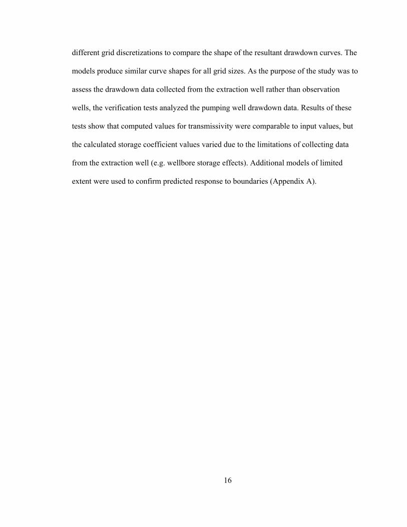
Simulations using pumping rates of 50, 100, and 1000 ft3/day (representing 2%,

4%, and 40% of total recharge) showed similar patterns in the drawdown and derivative

plots to those of the 600 ft3/day pumping-rate test seen in Figure 5-4 (Figure 5-5). Using

a lower pump rate produced only nominal change in the aquifer size, while the higher

1000 ft3/day rate generates a noticeable reduction in height (8 ft) and footprint (60 ft). All

tests exhibit a similar pattern of reduction in aquifer height and increased well drawdown

dominant in the early stages of the test followed by a pronounced reduction in total

leakage, analogous to the 600 ft3/day pump rate test. At the completion of the simulation,

the total reduction in leakage approached the respective pump rates for each test.

The drawdown and derivative curves for all well pumping rates also showed a

decrease in the rate of drawdown at late time, easily viewed as the derivative curve shifts

to a negative slope (Figure 5-5). The inflection point from positive to negative slope

developed earlier in the lower pump rates as less reduction in leakage volume was

required to offset the extraction rate. The ratios of the reduction of the total leakage rate

to extraction rate at the inflection points are 8% for the 50 ft3/day and 4% for the 100

ft3/day pump rates, comparable percentages to that observed in the 600 ft3/day pump rate.

In both tests, drawdown was observed at the aquifer periphery at approximately 20 days,

near the occurrence of inflection points on the derivative curve. However, as boundaries

would be expected to produce an increase in the derivative slope rather than the

prominent negative slope seen in the curves, the coincidence of the inflection point with a

fully engaged boundary is not related.

33

Figure 5-5. Log-Log plot of drawdown (black) and derivative (red) curves within the

production well for the circular perched aquifer model for pumping rates of (a) 50,

(b) 100, and (c) 1000 ft3/day. The production well was placed at the center of the

perched aquifer.

The overall response of the drawdown and derivative curves seen in the 1000

ft3/day pump rate test was analogous to previous examples, yet some differences were

1.0E-5 0.001 0.1 10. 1000.1.0E-4

0.01

1.

100.

Time (day)

Dra

wd

ow

n (

ft)

(a) 50 ft3/day Pump Rate Test

Drawdown Curve

Derivative Curve

1.0E-5 0.001 0.1 10. 1000.1.0E-4

0.01

1.

100.

Time (day)

Dra

wd

ow

n (

ft)

100ft3/day Pump Rate Test(b)

1.0E-5 0.001 0.1 10. 1000.1.0E-4

0.01

1.

100.

Time (day)

Dra

wd

ow

n (

ft)

(c) 1000ft3/day Pump Rate Test

34

observed. The first is the increase in fluctuations in the derivative curve. These were

likely numerical in origin, however they create uncertainties in identifying the inflection

point to a negative slope derivative curve. A second distinction from the previous tests is

the 0.2 positive slope of the derivative curve following the delayed-yield response. Two

differing physical mechanisms may contribute to this pattern. As the pump rate has

increased to 40% of the recharge rate, the extraction rate may be sufficiently large that

boundary effects were no longer obscured by recharge. Techniques utilized in curve

analysis describe flow regimes that depict positive slope-derivative curves, supporting the

assertion that the increasing derivative curve observed in this simulation results from

boundary effects (Cinco-Ley et al. 1981, Barker 1988). A second mechanism for the

positive slope-derivative curve was a reduction in transmissivity as the increase in

pumping rate created a thinner aquifer. This would increase the drawdown in the well. A

high rate produces a deepening of the cone of depression and effective reduction of

transmissivity at the wellbore (Hall 1996). Simple models were generated to assess the

effects of pumping on a thin aquifer (Appendix B). Results from simulations of an

infinite-in-extent unconfined aquifer of equivalent aquifer parameters produces a radial

flow drawdown and derivative curve at low pump rates and a 0.15 positive slope-

derivative curve at higher rates.

Off-Center Well Simulations

Placing the production well approximately 50 feet outside of the edge of the

recharge area produced similar results to those described above. All other conditions

remained the same. The observed physical processes suggest comparable behavior to the

center well location. The aquifer thickness was approximately 12 feet at the well. Due to

35

the reduced transmissivity as compared to the center well location, simulations were

conducted at lower pump rates of 100 and 300 ft3/day which represent 4 and 12% of the

total daily recharge rate, respectively. Figure 5-6 presents drawdown patterns through the

center of the circular aquifer using a pumping rate of 300 ft3/day after 1,000 days of

pumping.

Figure 5-6. Cross section through the center of the circular perched aquifer after

1,000 days of pumping at 300 ft3/day. The well is located 50 feet outside the recharge

area. Outline in background shows the initial shape of the aquifer.

The flow path arrows indicate that recharge was captured along the flanks of the

aquifer, eventually diminishing the supply of water to the down-gradient lobe. Initially,

there was a decrease in aquifer thickness followed by a footprint reduction as leakage and

pumping continually removed water from the system. A modest reduction in maximum

aquifer height at the center of the aquifer is observed to be 0.2 ft in the 100 ft3/ day test

Final Aquifer Outline

36

and 0.7 ft for the 300 ft3/day pump rate test. The time-drawdown and derivative behaviors

were similar to those seen in the center well locations (Figure 5-7). During the early time

period, the maximum height of the aquifer in the region of the well decreased which was

mirrored in the well drawdown. The reduction in total leakage rate began at early time,

increased throughout the test and approached the extraction rate at test completion. The

off-center well locations also showed footprint reduction.

Figure 5-7. Log-Log plot of drawdown (black) and derivative (red) curves within the

production well for the circular perched aquifer model for pumping rates of (a) 100

and (b) 300 ft3/day. The production well was placed at 50 feet away from the edge of

the recharge area.

The delayed-yield response was followed by the combined influences of pump

extraction, increased capture of recharge, and initial reduction of leakage producing a

near-horizontal curve at the lower pump rate and a positive slope at the 300 ft3/day pump

test. Derivative curves then increased in negative slope which coincided with footprint

reduction and increased reduction of total leakage rate. In the 100 ft3/day pump test, the

1.0E-5 0.001 0.1 10. 1000.1.0E-4

0.01

1.

100.

Time (day)

Dra

wd

ow

n (

ft)

Drawdown Curve

Derivative Curve

100 ft3/day Pump Rate Test(a) (b) 300 ft3/day Pump Rate Test

1.0E-5 0.001 0.1 10. 1000.1.0E-4

0.01

1.

100.

Time (day)

Dra

wd

ow

n (

ft)

37

reduction in total leakage rate was 7% of the extraction rate at 40 days. The fluctuations

in the 300 ft3/day pump rate test create uncertainties in identifying the inflection point for

the derivative curve. This point was approximately 60 days, corresponding to reduction in

total leakage rates of 16% of the extraction rate. Observation points along the aquifer

periphery near the pumping well (not shown) indicated initial drawdown at 8 days, and,

near the periphery on the opposite side of the extraction well at 26 days. Surprisingly, late

time boundary effects were still not prominently observed despite the closer proximity of

the boundary. However, the response of the positive slope derivative in the 300 ft3/day

off-center pump test presents issues analogous to those discussed in the 1000 ft3/day

center well pump test (i.e. decrease in saturated thickness proximal to the wellbore and

boundary influence no longer masked by recharge).

Edge Well Simulation

Simulations were also run placing the production well approximately 200 feet

from the center of the aquifer and 80 feet from the aquifer edge. The aquifer was 4.5 ft

thick at this location. Due to the decrease in transmissivity, the pump rate was reduced

and simulations were run on 10 and 40 ft3/day rates. To improve simulation results, the

grid spacing adjacent to the well was reduced from 5 ft to 2.5 ft. The cross section of the

40 ft3/ day pump test at test completion is shown in Figure (5-8).

38

Figure 5-8. Cross section through the center of the aquifer after 1,000 days of

pumping at 40 ft3/day. The well is located 150 feet outside of the recharge area.

Outline in background shows the initial shape of the aquifer.

Analogous to previous tests, simulations for both pump rates at the edge well

location showed comparable interactions and resulting drawdown and derivative patterns

(Figure 5-9). Again, the low pump rate produced a near-horizontal derivative curve while

the higher pump rate of 40 ft3/day resulted in a positive slope-derivative curve at late

time. Both simulations exhibit inflection points on the derivative curve once total leakage

rates were reduced. The 10 ft3/day pumping rate test showed an inflection point after the

reduction of the total leakage rate equaled 6% of the extraction rate. The 40 ft3/day

pumping rate test exhibited an inflection point once the reduction in the total leakage rate

was 25% of the extraction rate. Observation points at the periphery of the aquifer near the

edge well suggests the boundary was encountered at approximately 4.5 days and along

39

the edge on the opposite side of the pumping well at 45 days. However, the boundary

impact on the drawdown curve was indistinguishable from influences of recharge,

leakage, and pumping, except as previously noted in the higher pumping-rate tests.

Figure 5-9. Log-Log plot of drawdown (black) and derivative (red) curves within the

production well for the circular perched aquifer model for pumping rates of (a) 10

and (b) 40 ft3/day. The production well was placed approximately 200 feet from the

center of the aquifer.

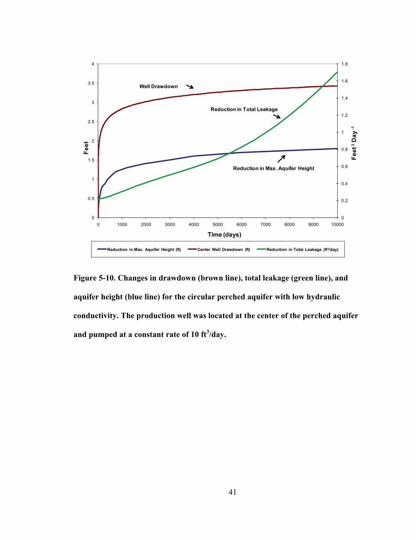
Tight-Aquifer Simulations

The results for the circular aquifer model using the lower hydraulic conductivity

of 0.2 ft/day exhibit similar relationships and patterns in the drawdown and derivative

curves to those observed in the higher hydraulic conductivity simulations. The sequence

of processes was comparable to the higher 3.0 ft/day hydraulic conductivity test

discussed above. However, in contrast to the 3.0 ft/day hydraulic conductivity models,

the lower hydraulic conductivity tests showed a continued increase in the total leakage

1.0E-5 0.001 0.1 10. 1000.1.0E-4

0.01

1.

Time (day)

Dra

wd

ow

n (

ft)

10ft3/day Pump Rate Test(a)

Drawdown Curve

Derivative Curve

1.0E-5 0.001 0.1 10. 1000.1.0E-4

0.01

1.

Time (day)D

raw

do

wn

(ft

)

(b) 40 ft3/day Pump Test

40

rate throughout the test indicating that the system never approached steady-state

conditions between pumping, leakage, and recharge (Figure 5-10). Leakage was

markedly less than total extraction rate after 10,000 days. Hydraulic resistance (ratio of

the thickness of the aquitard, b', to the hydraulic conductivity of the aquitard, K') serves

as an example of the impact in aquifer response due to the different hydraulic

conductivities. The hydraulic resistance is 1,000,000 days in the 0.2 ft/day hydraulic

conductivity model and 6,667 days in the 3.0 ft/day hydraulic conductivity model which

reflects a factor of 150 in the ability to transmit water through the aquitard. Figure 5-10

provides an example of the results found in the low hydraulic conductivity simulations.

Figure 5-11 depicts the drawdown and derivative curve. These figures convey the same

processes but the increased duration of the test required to produce an analogous response

to the higher hydraulic conductivity is greater than an order of magnitude.

41

Figure 5-10. Changes in drawdown (brown line), total leakage (green line), and

aquifer height (blue line) for the circular perched aquifer with low hydraulic

conductivity. The production well was located at the center of the perched aquifer

and pumped at a constant rate of 10 ft3/day.

0

0.2

0.4

0.6

0.8

1

1.2

1.4

1.6

1.8

0

0.5

1

1.5

2

2.5

3

3.5

4

0 1000 2000 3000 4000 5000 6000 7000 8000 9000 10000

Fe

et 3

Da

y -1

Fe

et

Time (days)

Reduction in Max. Aquifer Height (ft) Center Well Drawdown (ft) Reduction in Total Leakage (ft³/day)

Well Drawdown

Reduction in Total Leakage

Reduction in Max. Aquifer Height

42

Figure 5-11. Log-Log plot of drawdown (black) and derivative (red) curves within

the production well for the circular, 0.2 ft/day hydraulic conductivity, perched

aquifer model at 10 ft3/day pumping rate. The production well was in the center of

the aquifer.

Rectangular Model

The rectangular models were initialized in a comparable manner to the circular

models. The simulations started with a hydrostatic zero head on which a constant-rate

linear recharge was imposed to develop the rectangular perched aquifer. Simulations

using the 3.0 ft/day hydraulic conductivity aquifer reached quasi steady-state after 11

1.0E-5 0.001 0.1 10. 1000.0.001

0.1

10.

Time (day)

Dra

wd

ow

n (

ft)

10 ft3/day Pump Rate Test

Drawdown Curve

Derivative Curve

43

years. The lower hydraulic conductivity (K = 0.2 ft/day) perched aquifer models required

approximately 550 years to stabilize. These quasi steady-state heads were imported into

identical models and constant rate pumping tests were conducted in two differing well

locations within the perched aquifer. The model length was sufficient that the distal

boundaries of the model were not encountered by the radius of influence of the

production well. Table 4-1 and 4-2 provides the pumping rates and aquifer parameters.

Results for the rectangular models were comparable to the respective circular

models in the both the 3.0 ft/day and 0.2 ft/day hydraulic conductivity simulations. The

tight aquifer (K = 0.2 ft/day) required lower pumping rates to prevent dewatering and a

lengthy test duration (10,000 days) to produce comparable curve patterns to those

observed in the higher hydraulic conductivity simulations. Figure 5-12 shows the

drawdown and derivative curves for 3.0 ft/day hydraulic conductivity model for the

center and edge pumping locations. As the dominant physical processes were the same,

the drawdown response was analogous to the circular models. Again, a negative slope-

derivative curve developed as leakage in the region of the well was lessened by a

reduction in aquifer height and/or footprint. At higher rates or as the well was positioned

at the edge of the aquifer, a positive slope-derivative curve was again noted. Results

showed a positive slope-derivative curve of 0.5 to 0.6. Based on the results, the

mechanisms for the positive slope seen in the rectangular perched aquifer simulations

were as for those described for the circular perched aquifers. That is, the effects of

reduced transmissivity and increased boundary impact, produced indistinguishable

influences on the drawdown curve response.

44

Figure 5-12. Rectangular model center and edge well locations drawdown and

derivative curves for 100 ft3/day pump rate tests using an aquifer hydraulic

conductivity of 3.0 ft/day.

Transmissivity Estimates

As discussed above, the response of a perched aquifer to pumping produces a

complex time-drawdown. Nevertheless, the leaky perched aquifer simulations provided

an opportunity to evaluate a method to estimate transmissivity values. Below, we used

simulated time-drawdown data to develop a simplified methodology to measure aquifer

parameters yet may be applicable to field operations.

The preceding sections of this chapter have shown that the thickness of the leaky

perched aquifer changed as a result of spatial and temporal variations in head rendering

transmissivity a dynamic value. Therefore, seeking a single representative transmissivity

parameter for the perched system is of limited use. Analysis of the drawdown curves used

in this study suggests that the hydraulic conductivity is a more suitable parameter to

obtain from the drawdown curves. Knowing the estimated hydraulic conductivity allows

1.0E-5 0.001 0.1 10. 1000.1.0E-4

0.01

1.

Time (day)

Dra

wd

ow

n (

ft)

100ft3/day Pump Rate Test - Center(a)

1.0E-5 0.001 0.1 10. 1000.1.0E-4

0.01

1.

Time (day)

Dra

wd

ow

n (

ft)

(b) 100 ft3/day Pump Rate Test - Edge

45

for re-calculation of transmissivity values due to changes in aquifer thickness. Storage

values were also examined but did not provide useful results.

To assess hydraulic conductivity, the Cooper-Jacob straight-line method (Cooper

and Jacob 1946) with drawdown correction for unconfined aquifers (Jacobs 1944) was

found to produce consistent results. Figure 5-13 depicts the process to determine the

hydraulic conductivity. The figure presents semilog plots of the drawdown and derivative

curves for simulations conducted with the sand texture and center well location for two

pumping rates (50 ft3/day and 600 ft3/day). First, the time at which the delayed-yield

interval ends was located on the derivative curve; then the corresponding point on the

drawdown curve was found. The tangent line to this point was then estimated. The results

of the 50 ft3/day pumping-rate test showed that the gentle slope of the derivative curve

created difficultly in identifying the completion of delayed-yield response and thus the

point at which the straight line should be fit to the drawdown curve. As drawdown during

the pump test was low, fitting the curve further away from the end of the delayed-yield

response did not significantly affect the results. The 600 ft3/day pumping-rate test had an

easily identified point for the completion of the delayed yield. This point was then used to

establish the tangent line to the drawdown curve. Due to the physical processes

previously described in this study, the reducing slope of the drawdown curve near the

completion of the simulation deviated from the straight line.

The transmissivity value was determined for this tangent line in accordance with

the Cooper-Jacob straight-line method. By assuming that the loss of aquifer height was

negligible immediately following the delayed-yield component, the transmissivity value

was divided by the initial thickness of the perched aquifer to obtain hydraulic

46

conductivity (in field operations, the initial thickness of the perched aquifer would be

ascertained from drilling operations). To estimate transmissivity values at differing

locations within the perched aquifer or as a result of decreasing aquifer height from

pumping, the hydraulic conductivity value can be multiplied by various aquifer

thicknesses.

Using this technique, hydraulic conductivity for simulations in this study were

estimated. Table 5-1 and Figure 5-14 present the results. As shown, the hydraulic

conductivities were comparable to the simulation input values of 3.0 ft/day and 0.2 ft/day

for the fine sand and silt textures respectively. All results were slightly higher than the

input parameter, most notably in the higher pumping-rate simulations.

47

Figure 5-13. Examples of estimating the initial transmissivity value using the

Cooper-Jacob straight-line method. The semilog plots depict drawdown (black) and

derivative (red) curves from the circular aquifer, K = 3.0 ft/day, center well

locations. Upper plot is 50 ft3/day pumping rate and lower is 600 ft3/day pumping

rate.

1.0E-5 0.001 0.1 10. 1000.0.

0.32

0.64

Adjusted Time (day)

Co

rrec

ted

Dis

pla

cem

ent

(ft)

Obs. Wells

obs 1

Aquifer Model

Unconfined

Solution

Cooper-Jacob

ParametersT = 71.27 ft2/dayS = 1.972

Cooper-Jacob Straight Line

Start Straight-Line Segment

Point Following Delayed Yield

Co

rrec

ted

Dra

wd

ow

n (

ft)

50 ft3/day Pump Rate Test

Drawdown Curve

Derivative Curve

1.0E-5 0.001 0.1 10. 1000.0.

4.

8.

Adjusted Time (day)

Co

rre

cted

Dis

pla

cem

ent

(ft)

Obs. Wells

obs 1

Aquifer Model

Unconfined

Solution

Cooper-Jacob

Parameters

T = 74.77 ft2/dayS = 3.709

Cooper-Jacob Straight Line

Point Following Delayed Yield

Start Straight-Line Segment

Co

rrec

ted

Dra

wd

ow

n(f

t)

600 ft3/day Pump Rate Test

Drawdown Curve

Derivative Curve

48

Shape Tex Well

Loc.

Pump

Rate

(ft3/day)

Start

Time of

Straight

line

K

(ft/day)

b

(ft)

Predict.

T

(ft2/day)

Simul.

T

(ft2/day)

Simul.

K

(ft/day)

C S Cent 50 13 days 3.0 21 63 71 3.4

100 14 days 3.0 21 63 73 3.5

600 3 days 3.0 21 63 75 3.6

1000 2.6 days 3.0 21 63 80 3.9

Off-

Cent

50 7 days 3.0 12 36 38 3.1

100 3.6 days 3.0 12 36 41 3.3

300 4 days 3.0 12 36 44 3.6

Edge 10 0.6 days 3.0 4.7 14 16 3.3

40 0.5 days 3.0 4.7 14 17 3.7

Silt Cent 10 40 days 0.2 14 2.8 3.6 0.25

25 22 days 0.2 14 2.8 4.2 0.29

Off-

Cent

10 30 days 0.2 10 2.0 2.3 0.22

Edge 2 25 days 0.2 5.3 1.1 1.1 0.22

R S Cent 100 1.2 days 3.0 14 42 50 3.7

300 1 day 3.0 14 42 48 3.5

Edge 100 1 day 0.2 8.0 1.6 28 3.5

Silt Cent 2 25 days 0.2 12 2.4 2.6 0.22

Edge 2 30 days 0.2 6.1 1.2 1.3 0.22

Table 5-1. Computed and predicted transmissivity and hydraulic conductivity

values for simulations in this study. Abbreviations: C is circular; R is rectangular;

Tex is texture; S is sand; Loc. is Location; Cent is center; Predict is predicted; T is

transmissivity; b is aquifer thickness; K is hydraulic conductivity; Simul is

simulation.

49

Figure 5-14. Estimated hydraulic conductivity values for simulations presented in

this study using the Cooper-Jacob straight-line method tangent to the drawdown

curve immediately following the delayed-yield response. Values adjacent to the data

point represent the simulation pumping rate in ft3/day. The squares and circles

represent the high (3.0 ft/day) and low (0.2 ft/day) hydraulic conductivity model

runs, respectively.

Applicability of Time Constraints to Field Investigations

Results from this study have shown that the drawdown curves from constant-rate

pump tests can assist in differentiating a leaky perched aquifer from an infinite in areal

extent aquifer by the appearance of a negative slope-derivative curve. Furthermore,

0

0.2

0.4

2.9

3.1

3.3

3.5

3.7

3.9

K= 3 ft/day

Circular RectangularRectangular CircularSilt Texture, K= 0.2 ft/dayFine Sand Texture, K= 3 ft/day

K= 0.2 ft/day

CenterCenter CenterCenterOff-

CenterOff-Center

Edge Edge Edge Edge

300

100

300

50

100

600

1000

10

100

10

50

40

100

2510 22 2

Hyd

rau

lic

Co

nd

uct

ivit

y, K

(ft

/day

)

50

simulation results suggest that the drawdown and derivative curves provide a reliable

hydraulic conductivity to permit the calculation of the varying transmissivity. For these

findings to be of value to field investigations, the data must be obtained within practical

time constraints.

Although the silt model (hydraulic conductivity of 0.2 ft/day) required excessive

test durations (~2,000 days), the fine sand model (hydraulic conductivity of 3.0 ft/day)

produced informative results within reasonable time intervals (~20 days). Simulations

demonstrated that the appearance of the negative slope-derivative curve suggesting a

leaky perched aquifer formed earlier at low pumping rates as the aquifer did not require a

large reduction in size to approach a new equilibrium. Therefore, by use of low extraction

rates, the first appearance of the negative slope on the derivative curve was achieved

within plausible time periods for field tests. Figure 5-5 shows an example of the onset of

the inflection point and differing pumping rates. In the 50 ft3/day pumping-rate test, the

inflection point is located at approximately 20 days, an order of magnitude less than that

of the 1,000 ft3/day pumping-rate test.

The response of the aquifer to constant pumping is observed sooner in higher

hydraulic conductivity formations. When the models presented in this investigation were

scaled to higher hydraulic conductivities, comparable leaky perched aquifers were

generated. Figure 5-15 shows an example where the hydraulic conductivity of the

perched aquifer was increased from 3.0 ft/day to 300 ft/day with other model parameters

scaled accordingly. The drawdown and derivative curves show analogous patterns to the

hydraulic conductivity of 3.0 ft/day but developing over a shorter duration.

51

Therefore, the 3.0 ft/day hydraulic conductivity tested in this study yielded a

negative slope-derivative curve in a reasonable time period if the low pumping rates were

used. However, these results may represent the lower range of transmissivities capable of

producing meaningful results within acceptable time constraints for field applications.

Higher hydraulic conductivity formations required less time to obtain useful data due to

the faster response of the formation.

Figure 5-15. Log-Log drawdown and derivative curve for the constant-rate pump

test conducted in a simulated perched aquifer of hydraulic conductivity 300 ft/day

resulting in a shorter duration for the completion of the delayed-yield response and

development of the negative slope-derivative curve.

As discussed in the preceding section, using the Cooper-Jacob straight-line

method provided reasonable estimates of hydraulic conductivity that could then be used

1.0E-5 0.001 0.1 10. 1000.1.0E-4

0.01

1.

100.

Time (day)

Dra

wd

ow

n (

ft)

K = 300 ft/dayPumping Rate = 60,000 ft3/day

Drawdown Curve

Derivative Curve

52

to assess the variable transmissivity. As the point from which the straight line was

determined was obtained immediately following the delayed-yield response, all time

periods for models using the hydraulic conductivity of 3.0 ft/day were practical for field

applications. The hydraulic conductivity values were closest to the predicted parameter at

lower pump rates, further supporting the use of reduced pumping rates in field operations.

53

CHAPTER 6 - CONCLUSIONS

The purpose of this study was to ascertain if particular and unique responses of a

constant-rate pump test in a leaky perched aquifer receiving recharge can identify the

aquifer: 1) as limited in lateral extent, 2) of a particular geometry, and 3) the well position

within the perched aquifer. Simulation results showed a consistent late-time response that

identified the limited size of the perched aquifer. Specifically, the simulations showed

extraction demands were initially met by recharge and storage. As less recharge was

available to sustain the aquifer due to pumping and continued leakage through the

aquitard, the size of the aquifer diminished by a decrease in lateral footprint and/or

thickness. The reduced size of the aquifer and reduced head lessened the total volume

leaked through the aquitard, which provided more recharge water to meet the demands,

reducing the rate of drawdown in the well as the system approached a new steady-state.

The decrease in rate of drawdown is expressed as a negative slope on the derivative

curve. Figure 6-1 depicts the generalized contribution of sources delivered to the well and

corresponding response of the drawdown curve. The well supply at early time (A) was

met from wellbore and elastic storage. Following this period, a delayed-yield response

was observed indicating the dominance of water delivered to the well from specific yield

(B), after which the expanding cone of depression provided a greater component by

increased interception of recharge entering the perched aquifer. Over time, the expanding

54

cone of depression and capture of recharge delivered the bulk of water to the well (C),

and, as the aquifer size was further reduced, the system approached equilibrium (D).

Figure 6-1. Schematic of water sources to the well and corresponding drawdown

and derivative curve. The lag time of the delayed-yield component is not

incorporated in the water source graph. Segments A, B, C, and D represent major

shifts in the well supply and drawdown curve.

1.0E-5 0.001 0.1 10. 1000.1.0E-4

0.01

1.

100.

Dra

wd

ow

n (

ft)

Drawdown Curve

Derivative Curve

600 ft3/day Pump Rate

A B C D

55

It is the constrained size of the leaky perched aquifer with constant recharge that

allows for the development of a new equilibrium by reduction of the aquifer size. As the

system approaches a new steady-state, a decrease in the rate of drawdown is observed in

the extraction well. This repeatable pattern of a late time negative slope-derivative curve

is in contrast to the infinite-in-extent unconfined aquifer seen in Figure 1-2(a) where the

derivative curve shows a late time horizontal line identifying radial flow associated with

infinite-in-extent aquifers.

Thus, the first objective of the study is met as the observation of the negative

slope-derivative curve can assist in differentiating a leaky perched aquifer receiving

recharge from an infinite-in-extent unconfined aquifer. However, the remaining goals of

ascertaining the geometry and position of the well within the perched aquifer were not

achieved as the simulations indicate that boundary effects and aquifer geometry are

masked by other late-time processes.

As depicted in all the simulations, the overriding mechanism at late time is the

increased capture of recharge, reduction of aquifer size, and decrease in total leakage

providing an increase in water supply to the well. It is the response of the drawdown

curve to this mechanism that dominates the behavior of the curve. The system is dynamic

and the changing impact of recharge, leakage, pumping, and boundaries combine to

create the appearance of the drawdown and derivative curves.

Data obtained from this study presented an opportunity to examine a method for

estimating transmissivity. An evaluation of the simulated drawdown curves using the

Cooper-Jacob straight-line method was conducted on the tangent to the point

56

immediately following the delayed-yield effect. Aquifer test-analysis using this straight-

line slope produced comparable hydraulic conductivity values to the model input

parameters. Determining the hydraulic conductivity allows transmissivity values to be

calculated according to the spatial and temporal changes of aquifer thickness in the leaky

perched aquifer.

As the simulations were conducted using low pumping rates with small

drawdowns over lengthy test durations, the results of this study were reviewed for

feasibility to field investigations. Assessments showed the small drawdown in the

pumping well can be measured using appropriate field equipment and by use of low

pumping rates the duration to obtain meaningful data is achieved within practical time

periods for field operations. The lower pumping rates required less reduction in aquifer

size for the system to return to equilibrium, therefore, the appearance of the negative

slope-derivative curve developed sooner than for simulations at higher pumping rates.

Additional considerations supporting the use of a low pumping rate for fieldwork were

the improved hydraulic conductivity estimates as compared to those obtained from higher

pumping rates and the avoidance of a positive slope-derivative curve. Tests showed that a

thin, infinite-in-extent aquifer could exhibit a positive slope-derivative curve at high

pump rates. As a positive slope-derivative curve is often attributed to boundary

influences, the use of a lower pump rate may avoid erroneous identification of aquifer

boundaries when the system is actually an infinite-in-extent aquifer.

Components of this study may be extended to perched aquifers formed by

differing hydrological environments. For example, a perched aquifer formed on a

localized aquitard with recharge covering most of the perched zone would likely develop

57

comparable drawdown patterns. In this case, leakage would be replaced by groundwater

movement over the periphery of the aquitard. However, given the diversity of features

that may be involved in the development of a perched aquifer, additional numerical

exploration to determine the resultant drawdown curves is merited. Although the systems

described are highly nonlinear, investigation into the development analytical solutions

focusing on leakage and pumping effects should be considered.

58

REFERENCES

Anakhaev, K.N. 2009. A particular analytical solution of a steady-state flow of a

groundwater mound. Water Resources. 36 (5) pp.507-512.

Bagtzoglou, A.C. 2003. Perched water bodies in arid environments and their role as

hydrologic constraints for recharge rate estimation: Part 1. A modeling

methodology. Environ. Forensics v. 4(1), p. 39-46.

Barker, J.A. 1988. A generalized radial-flow model for pumping tests in fractured rock.

Water Resources Research. 24, 1796-1804.

Behera, S., Jha, M.K., Kar, S. 2003. Dynamics of water flow and fertilizer solute leaching

in lateritic soils of Kharagpur region, India. Agricultural Water Management.

63(2), p.77-98.

Boulton, N.S. 1954. The drawdown of the water-table under non-steady conditions near a

pumped well in an unconfined formation. Proceedings of the Institution of Civil

Engineers, London, great Britain, Part III, p.564-579.

59

Bourdet, D., Ayoub, J.A., Pirard, Y. M. 1989. Use of pressure derivative in well-test

interpretation. Society of Petroleum Engineers Formation Evaluation. June. 293-

302.

Bouwer, H., Back, J., Oliver, J.M. 1999. Predicting infiltration and ground-water mounds

for artificial recharge. Journal of Hydrological Engineering. 4 (4), pp. 350-357.

Cinco-Ley, H., Samaniego-V. F. 1981. Transient pressure analysis for fractured wells.

Journal of Petroleum Technology. September. 1749-1766.

Cooper, H.H., Jacob, C.E. 1946. A generalized graphical method for evaluating

formation constants and summarizing well field history, Transactions, American

Geophysical Union. 27, p.526-534.

Cozzarelli, I.M., Herman, J.S., Baedecker, M.J. Fischer, J.M. 1999. Geochemical

heterogeneity of a gasoline-contaminated aquifer. Journal of Contaminant

Hydrology. 40 (3) , pp.261-284.

Driscoll, F.G. 1986. Groundwater and Wells, Second Edition. U.S. Filter/Johnson

Screens, St. Paul, Minnesota. 1089 p.

Duffield, G.M. 2007. AQTESOLV for Windows Version 4.5. User's Guide,

HydroSOLVE, Inc., Reston, Virginia.

60

Ferris, J.G., Knowles, D.B., Brown, R.H., Stallman, R.W. 1962. Theory of aquifer tests.

U. S. Geological Survey Water-Supply Paper. 1536-E, 69-174.

Fetter, C.W. 1994. Applied Hydrogeology, third edition. Macmillan College Publishing

Company, New York, N.Y. 691p.

Fogg, G.E., Fleckenstein, J., Niswonger, R.G., Rains, M.C., and Williamson, R.J. 2003.

Perched aquifer hydrology: An Unexplored Frontier? Geological Society of

America Abstracts with Programs, Vol. 35, No. 6, September 2003, p.449.

Hall, P. 1996. Water Well and Aquifer Test Analysis. Water Resources Publications,

LLC, Highlands Ranch, Colorado. 412 p.

Hantush, M.S., Jacob, C.E. 1955. Non-steady radial flow in an infinite leaky aquifer.

Transactions, American Geophysical Union. 36 (1), 95-100.

Hueni, C. 2010. Current Status Report: Pantex Plant (USDOE), EPA ID # TX4890110,

Site ID 0604060, EPA region 6. url:

http://www.epa.gov/region6/6sf/pdffiles/0604060.pdf. Accessed December 20.

2010.

HydroGeoLogic, Inc. 2007. MODFLOW-SURFACT Software (Version 3.0) Overview:

61

Installation, Registration and Running Procedures. Herndon,

VA.<www.hgl.com>.

Jacob, C.E., 1944. Notes on determining permeability by pumping tests under water-table

conditions. U.S. Geological Survey Mimeo Report, US Geological Survey,

Reston, VA.

McDonald, M.G., Harbaugh, A.W., 1988. A modular, three-dimensional finite difference

ground-water flow model: US Geological Survey Techniques of Water-Resources

Investigations, book 6, chap.A1. 586 p.

Moench, A.F.1995. Combining the Neuman and Boulton models for flow to a well in an

unconfined aquifer. Ground Water. 33(3), p. 378-384.

Neuman, S.P. 1972. Theory of flow in unconfined aquifers considering delayed response

of the water table. Water Resources Research. 8 (4), 1031-1044.

Neuman, S.P. 1974. Effect of partial penetration on flow in unconfined aquifers

considering delayed gravity response. Water Resources Research. 10 (2), 303-

312.

62

Panday, S., Huyakorn, P.S. 2008. MODFLOW SURFACT: A state-of-the-art use of

vadose zone flow and transport equations and numerical techniques for

environmental evaluations. Vadose Zone Journal. 7 (2), 610-631.

Phillips, Owen M. 1991. Flow and Reactions in Permeable Rocks. Cambridge University

Press, New York, NY. 285 p.

Rains, M.C., Fogg, G.E., Harter, T., Dahlgren, R. A., Williamson, R.J., 2006. The role of

perched aquifers in hydrological connectivity and biogeochemical processes in

vernal pool landscapes, Central Valley, California. Hydrological Processes. 20.

1157-1175.

Reichard, E.G., Izbicki, J.A., Martin, P. 1995. Implications of uncertainty in exposure

assessment for groundwater contamination. Proceeding from the Rome

Symposium, September 1994, Assessing and Managing Health Risks from

Drinking Water Contamination: Approaches and Applications. IAHS Publ. no

235, pp. 211-219.

Renard, P., Glenz, D., Mejias, M. 2009. Understanding diagnostic plots for well-test

interpretation. Hydrogeology Journal. 17, 589-600.

Schlumberger, 2009. Visual MODFLOW Software (Version 2009.1 Pro) Developed by

Schlumberger Services.

63

Schwartz, F.W., Zhang, H. 2003. Fundamentals of Ground Water. John Wiley & Sons,

New York, NY. 583 p.

Serrano, Sergio E. 2003. Modeling groundwater flow under transient nonlinear free

surface. Journal of Hydrologic Engineering.8(3), p.123-132.

Theis, C.V. 1935. The relationship between lowering of the piezometric surface and the

rate and duration of discharge of a well using groundwater storage. Transactions,

American Geophysics Union. 16, 519-524.

Walker, D.D., Roberts, R.M. 2003. Flow dimensions corresponding to hydrogeologic

conditions. Water Resources Research. 39 (12), 1349-1356.

Wu, Y.S., A.C. Ritcey, and G.S. Bodvarsson. 1999. A modeling study of perched water

phenomena in the unsaturated zone at Yucca Mountain. Journal Contam. Hydrol.

V. 38 (1-3), p. 157-184.

64

APPENDIX A - VERIFICATION OF MODELING SOFTWARE

The MODFLOW-SURFACT (HydroGeoLogic, Inc. 2007) simulations and

Aqtesolv (Duffield 2007) drawdown and time-derivative curves were verified for the

ability of the software to produce the predicted aquifer parameters and the anticipated

response to boundaries when constant-rate pump tests were imposed. Two sets of simple

rectangular models were constructed. The first group simulated aquifers of infinite areal

extent to assess predicted versus computed parameter estimation. The second set of

models assessed an aquifer of limited extent for appropriate drawdown and derivative

curve behavior when the cone of depression uniformly encountered model no-flow

boundaries.

Infinite-in-Extent Models

Analytical solutions and the graphical depictions, or type curves, are used to

determine the transmissivity of an aquifer by comparing drawdown curves generated

from constant-rate pump tests to the analytically derived type curves. The solutions

assume infinite-in-extent aquifers. To verify the ability of the software to produce

transmissivity values comparable to those calculated from the input parameters, this type-

curve matching technique was performed on simulated data generated from models

mimicking infinite-in-extent conditions. The dimensions for the infinite areal extent

model were 20,000 ft in length (L) by 20,000 ft in width (W) by 10 ft in height (H).

65

Model layers were 1 ft thick. The vertical sequence of the model was composed of a 9 ft

thick aquifer overlying a 1 ft thick low permeability unit. The use of the low permeability

unit for the lowermost layer of the model improved the mass balance results. The

overlying layers composing the aquifer were constructed using the following parameters:

hydraulic conductivity, 3.0 ft/day; transmissivity, 27 ft2/day; specific yield (Sy), 0.3;

specific storage (Ss), 6E-6 ; and effective porosity, 0.3. Well casing and screen radii

were 0.3 ft and 0.25 ft, respectively. The pumping well was fully penetrating. The

extraction rate was 20 ft3/day for all simulations. The model boundaries were no-flow and

the initial head was set at the upper surface of the model for all cells. The cell size was

smallest in the region of the well increasing in size towards the model boundaries. Four

models were created based on the smallest grid size of the model: 0.8 ft; 1.6 ft; 6.3 ft;

and, 12.6 ft. Discretization for each model is shown in Table A-1. As the grid size

increased moving outwards from the pumping well, the minimum and maximum grid size

for each model is included in Table A-1. Models were run for 125 to 400 days and

achieved successful mass balance results.

Minimum

Grid Size

(ft)

Maximum

Grid Size

(ft)

Duration

(days)

% Mass

Balance

Discrepancy

Number of

Rows

Number of

Columns

Number of

Layers

0.8 ~ 1600 400 3.59 390 389 10

1.6 ~ 800 125 5.59 161 143 10

6.3 ~ 500 125 4.69 277 277 10

12.6 ~ 500 125 4.77 246 245 10

Table A-1. Summary of the infinite areal extent verification models discretization.

66

Drawdown data was collected at the pumping well and imported into Aqtesolv for

preparation and analysis of drawdown and derivative curves to assess predicted versus

computed transmissivity and storage values. Type-curve matching to obtain the computed

aquifer parameters was conducted using either the Neuman (1974) analytical solution for

unconfined aquifers with instantaneous delayed gravity drainage or the Cooper-Jacob

straight-line method (1946) with drawdown corrected for unconfined aquifers (Jacob

1944). The transmissivity value and specific yield values used by MODFLOW-

SURFACT were 27 ft2/day and 0.3, respectively. Aqtesolv provided an output of

storativity denoted as "S". Storativity for an unconfined aquifer is the sum of specific

yield and the product of specific storage (Ss) times the thickness of the aquifer (b):

)( bSsSyS ×+= A (1)

For the Neuman solution, storativity is the component under confined conditions

or specific storage times the aquifer thickness. For the Cooper-Jacobs straight-line

method, storativity is as shown in equation A(1). The value of S used in the MODFLOW-

SURFACT data set was 5.4E-5 for the Neuman solution and 0.300054, or approximately

0.3 for the Cooper-Jacob method. Since output taken at the extraction well included

wellbore storage effects, simulated storage values were anticipated to deviate from the

predicted values. The drawdown curves and analyses are presented below. As the results

slightly differ between the grids sizes, the 0.8 ft and 1.6 ft grids are discussed first with

the 6.3 ft and 12.6 ft grids following.

The smaller grid sizes (0.8 ft and 1.6 ft) produced drawdown and derivative

curves well matched to the respective type-curves (Figures A-1 and A-2). Table A-2

67

summarizes the simulated parameter results. The 0.8 ft grid was run for 400 days to

clarify late time derivative curve undulations as likely forming from numerical issues.

Therefore, at smaller grid sizes, the predicted and computed results for transmissivity

were comparable.

68

Figure A-1. Log-Log drawdown and derivative curves for the verification testing of

a constant-rate pump test. Thin, solid lines denote type curves. Estimated parameter

results using the Neuman (1974) solution for an unconfined aquifer are presented to

the right of the time-drawdown plot. The simulated time-drawdown data was from

the MODFLOW-SURFACT simulation using a grid size range of 0.8 ft at the well

expanding to ~1600 ft at model boundaries.

1.0E-6 1.0E-4 0.01 1. 100.1.0E-4

0.01

1.

Time (day)

Dra

wd

ow

n (

ft)

Obs. Wells

GRID 0.8 ft

Aquifer Model

Unconfined

Solution

Neuman

Parameters

T = 25.78 ft2/dayS = 8.496E-5Sy = 0.2649ß = 0.0007716

Drawdown curve – type curve solid line

Derivative curve – type curve solid line

69

Figure A-2. Log-Log drawdown and derivative curves for the verification testing of

a constant-rate pump test. Thin, solid lines denote type curves. Estimated parameter

results using the Neuman (1974) solution for an unconfined aquifer are presented to

the right of the time-drawdown plot. The simulated time-drawdown data was from

the MODFLOW-SURFACT simulation using a grid size of 1.6 ft at the well

expanding to ~800 ft at model boundaries.

70

Smallest Grid Size (ft)

Simulated T Value (ft2/day)

Percent Discrepancy of Simulated T from Predicted Value of 27ft2/day (%)

Simulated Sy Value

Percent Discrepancy of Simulated Sy from Predicted Value of 0.3 (%)

Simulated S (Ss *b)

Percent Discrepancy of Simulated S from Predicted Value of 5.4E-5 (%)

0.8 ft 25.78 4.5 0.2649 11.7 8.496E-5 57.3

1.6 ft 28.72 6.3 0.2414 19.5 8.496E-5 57.3

Table A-2. Summary of estimated parameter results for the finer grid models in the

infinite areal extent verification models. Parameters estimated using the Neuman

solution for an unconfined aquifer (1974). Abbreviations used: T is transmissivity,

Sy is specific yield, Ss is specific storage, b is aquifer thickness, and S is storativity.

Figures A-3 and A-4 show the 6.3 and 12.6 ft grid tests. Separation is observed

between the computed drawdown curve and the type-curves derived from input

parameters. These type curves demonstrate the deviation of the computed response from

the ideal type-curve response for the parameters used in the MODFLOW-SURFACT

simulation. The larger grids also produced a compression of the delayed yield component

followed by the development of a unit slope derivative curve into the late time interval.

At larger grid sizes, curve matching using the Neuman solution was not effective. Given

the poor results, the large grids were also analyzed using the Cooper-Jacob straight-line

method (1946). Using the Jacob (1944) method, the drawdown was corrected for an

unconfined aquifer. These analyses provided computed transmissivity values near

predicted results for late time data (Table A-3). The increased grid size distorted the early

and intermediate time results, with the late time curve response producing comparable

71

transmissivity values to that of a finer grid discretization. This implies the late time curve

behavior was less sensitive to the larger grids (up to 10 and possibly 20 feet). The late

time stability of the curve response suggests that the small variations in the grid size that

were required to optimize the leaky perched aquifer simulations did not influence the late

time curve behavior. This is important as the late time interval was the dominant period

over which the simulations were analyzed. It should be noted that discrepancies persisted

in storage values.

Grid Simulated

T Value (ft2/day)

Percent Discrepancy of Simulated T from Predicted Value of 27ft2/day (%)

Simulated S Value S= Sy+(Ss*b)

Percent Discrepancy of Simulated S from Predicted Value of ~ 0.3 (%)

6.3ft 28.21 4.48 4.835 ~1400 12.6 ft 27.65 2.4 27.18 ~9000

Table A-3. Summary of estimated parameter results for the larger grid models in

the infinite areal extent verification models. Parameters estimated using the Cooper-

Jacob straight-line method. Abbreviations used: Abbreviations used: T is

transmissivity, Sy is specific yield, Ss is specific storage, b is aquifer thickness, and S

is storativity.

72

Figure A-3. Log-Log drawdown and derivative curves for the verification testing of

a constant-rate pump test. Thin, solid lines are type curves corresponding to the

predicted parameters presented to the right of the time-drawdown plot. The

simulated time-drawdown data was from the MODFLOW-SURFACT simulation

using a grid size of 6.3 ft at the well expanding to ~ 500 ft at the model boundaries.

(c)

1.0E-8 1.0E-6 1.0E-4 0.01 1. 100.1.0E-4

0.01

1.

Time (day)

Dra

wd

ow

n (

ft)

Obs. Wells

obs well

Aquifer ModelUnconfined

Solution

Neuman

Parameters

T = 27. ft2/dayS = 5.4E-5Sy = 0.3ß = 0.0007716

6ft grid

Derivative curve type curve solid line

Drawdown curve type curve solid line

73

Figure A-4. Log-Log drawdown and derivative curves for the verification testing of

a constant-rate pump test. Thin, solid lines are type curves corresponding to the

predicted parameters presented to the right of the time-drawdown plot. The

simulated time-drawdown data was form the MODFLOW-SURFACT simulation

using a grid size of 12.6 ft at the well expanding to 500 ft at the model boundaries.

(d)

1.0E-8 1.0E-6 1.0E-4 0.01 1. 100.1.0E-4

0.01

1.

Time (day)

Dra

wd

ow

n (

ft)

Obs. Wells

obs well

Aquifer Model

Unconfined

Solution

Neuman

Parameters

T = 27. ft2/dayS = 5.4E-5Sy = 0.3ß = 0.0007716

12 ft grid

Drawdown curve type curve solid line

Derivative curve type curve solid line

74

Figure A-5. Semilog drawdown and derivative curves for the verification testing of a

constant-rate pump test. Analysis using Cooper- Jacob straight-line method. Thin,

solid lines denote type curves. Estimated parameters are presented to the right of

the time-drawdown plot. The simulated time-drawdown data was from the

MODFLOW-SURFACT simulation using a grid size of 6.3 ft at the well expanding

to ~ 500 ft at the model boundaries.

1.0E-8 1.0E-6 1.0E-4 0.01 1. 100.0.

0.24

0.48

Adjusted Time (day)

Eq

uiv

alen

t D

raw

do

wn

(ft

)

Obs. Wells

GRID 6 ft

Aquifer Model

Unconfined

Solution

Cooper-Jacob

Parameters

T = 28.21 ft2/dayS = 4.835

Co

rrec

ted

Dra

wd

ow

n (

ft)

Time (day)

75

Figure A-6. Semilog drawdown and derivative curves for the verification testing of a

constant-rate pump test. Analysis using Cooper- Jacob straight-line method. Thin,

solid lines denote type curves. Estimated parameter results are presented to the

right of the time-drawdown plot. The simulated time-drawdown data was form the

MODFLOW-SURFACT simulation using a grid size of 12.6 ft at the well expanding

to 500 ft at the model boundaries.

Limited-in-Extent Models

As perched aquifers are of limited areal extent, the ability of the software to

capture drawdown patterns associated with boundaries was verified. Small models (100 ft

(L) by 100 ft (W) by 20 ft (H)) were developed such that the model no-flow boundaries

would be encountered during the pump test. Three models were used to test grid sizes of

1.0E-8 1.0E-6 1.0E-4 0.01 1. 100.0.

0.2

0.4

Adjusted Time (day)

Eq

uiv

alen

t D

raw

do

wn

(ft

)

Obs. Wells

GRID 12.6 ft

Aquifer Model

Unconfined

Solution

Cooper-Jacob

Parameters

T = 27.65 ft2/dayS = 27.18

Co

rrec

ted

Dra

wd

ow

n (

ft)

Time (day)

76

0. 7 ft, 5 ft, and 10 ft on producing the anticipated drawdown and derivative curves. The

5 ft and 10 ft grid models had uniform grid spacing, while the 0.7 ft grid model utilized

small grid spacing in the region of the well that became coarser moving towards the

boundaries. Layer thicknesses were variable, ranging from 0.5 to 2 ft thick. The same

aquifer parameters were used as for the infinite-in-extent models described above. The

pumping rate was 200 ft3/day for 125 days. Drawdown results were imported into

Aqtesolv and are shown below.

Boundaries were observed in all models, as shown by the increase in drawdown

and unit slope derivative at late time. In these small extent models, the no-flow

boundaries surrounding the aquifer allow for the drainage of the system in an analogous

manner to wellbore storage effects that produce a unit slope drawdown and derivative

curve on the log-log plots. As shown by Renard et al. (2009), wellbore storage is

comparable to a well drilled in an aquifer having zero transmissivity. The derivative

curve and drawdown curve are of unit slope as:

tr

Qts

2π=)( (A-2)

Where Q is pumping rate, t is time, r is radius of well casing, s is drawdown.

The derivative of drawdown with respect to the natural logarithm of time (ln t) is the

derivative curve used in this study and is shown to equal the drawdown in the well as a

function of time:

)(ln 2

tsr

Qt

dt

dst

td

ds ===π (A-3)

77

Taking the logarithm of the above shows the derivative and the drawdown both equal to a

line of unit slope when plotted on log-log scale with log [s(t)] on the y axis and log(t) on

the x axis:

]log[)log(]ln

log[)](log[2r

Qt

td

dsts

π+== (A-4)

The limited-in-extent models behave in a similar manner to the wellbore storage

described above with the casing radius analogous to the distance to the model boundaries,

draining in a comparable pattern.

The results indicate the variation in the grid sizes did not influence the appearance

of the boundary effect.

Figure A-5. Log-Log drawdown and derivative curves for verification testing of

curve response to encountering model no-flow boundaries. The MODFLOW-

SURFACT grid varied between 0.7 ft at the well expanding to 5.0 ft at the model

boundaries.

1.0E-6 1.0E-4 0.01 1. 100.0.001

0.1

10.

Time (day)

Dra

wd

ow

n (

ft)

Drawdown Curve

Derivative Curve

(a) 0.7 ft Grid

78

Figure A-6. Log-Log drawdown and derivative curves for verification testing of

curve response to encountering model no-flow boundaries, 5 ft grid.

Figure A-7. Log-Log drawdown and derivative curves for verification testing of

curve response to encountering model no-flow boundaries, 10 ft grid.

1.0E-6 1.0E-4 0.01 1. 100.0.001

0.1

10.

Time (day)

Dra

wd

ow

n (

ft)

(b) 5ft Grid

1.0E-6 1.0E-4 0.01 1. 100.0.001

0.1

10.

Time (day)

Dra

wd

ow

n (

ft)

(c) 10 ft Grid

79

APPENDIX B - ADDITIONAL MODELS

Results from the leaky perched aquifer simulations conducted at high pump rates

show a positive slope-derivative curve. While the appearance of a positive slope-

derivative suggests boundary influences, observations during this study indicated a

reducing transmissivity could also contribute to a positive slope-derivative curve. Low

transmissivity and high pump rates each lead to a deepening of the cone of depression at

the wellbore (Hall 1996). This implies that a thin, low permeable aquifer subjected to

high pumping rates will experience a decreasing transmissivity as the aquifer height is

lowered in the region of the well, and therefore, an increase in drawdown. To determine

the influence of reduced transmissivity at the wellbore, constant-rate pump tests were

simulated in a thin, infinite-in-extent, unconfined aquifer. The model was 100,000 ft (L)

by 100,000 ft (W) by 10 ft (H) with parameters the same as the circular leaky perched

aquifer, 3.0 ft/day hydraulic conductivity model. Grid size was refined at the pumping

well. A series of three models were developed, defined by the smallest grid spacing: 4 ft;

6 ft; and 12 ft. The grid size increased outwards to a maximum grid size of 500 ft for all

models. Testing various grid sizes was conducted as issues of dewatering can arise from

numerical limitations when a high pumping rate in a low transmissivity unit is unable to

extract sufficient water over the time step. Increasing the grid size was found to alleviate

the dewatering. Therefore, testing of differing grid sizes was included to ensure that the

80

development of a positive slope-derivative curve was not the product of a tight grid size.

The models were run at pump rates 200 ft3/day. The infinite-in-extent model sequence

produced a slightly positive slope-derivative curve for all grid sizes (a slope of

approximately 0.15). A lower pump rate test of 20 ft3/day was conducted using the 6 ft

grid for comparison. The low pump rate showed a horizontal derivative indicative of

radial flow (Renard et al. 2009 ). Boundaries were not encountered in any simulation,

suggesting the positive slope-derivative curve resulted from a higher pumping rate that

induced an increasing rate of drawdown to meet well demands. The results of the pump

tests demonstrate the ability to produce a positive slope-derivative curve from a reduced

transmissivity at the wellbore, a product of the reduced thickness as water was removed

from storage to meet the higher pump demands.

81

Figure B-5. Log-Log drawdown and derivative curves for the unconfined, infinite in

areal extent models 200 ft3/day pumping-rate tests with a grid spacing of (a) 4 ft, (b)

6 ft and (c) 12 ft. The 20 ft3/day pumping-rate test with a grid spacing of 6 ft is

shown in (d).

1.0E-6 1.0E-4 0.01 1. 100.0.001

0.1

10.

Time (day)

Dra

wd

ow

n (

ft)

(a)

Drawdown Curve

Derivative Curve

1.0E-6 1.0E-4 0.01 1. 100.1.0E-4

0.01

1.

Time (day)

Dra

wd

ow

n (

ft)

(b)

1.0E-6 1.0E-4 0.01 1. 100.0.001

0.1

10.

Time (day)

Dra

wd

ow

n (

ft)

(c)

1.0E-6 1.0E-4 0.01 1. 100.1.0E-4

0.01

1.

Time (day)

Dra

wd

ow

n (

ft)

(d)