Embed Size (px)
Citation preview
DripDrop: A Dynamic Load Balancer & Autoscaler for DigitalOcean
Sukrit Handa University of Toronto
Toronto,ON [email protected]
Jake Stolee University of Toronto
Toronto,ON [email protected]
Abstract
DigitalOcean is a leading cloud computing platform which allows customers to manually create and manage VMs (or “Droplets”) [1]. Unfortunately, DigitalOcean currently does not provide services to automatically scale web application Droplets. In this report, we propose DripDrop, an autoscaler and dynamic load balancer for DigitalOcean. DripDrop is designed to automatically add and remove Droplets based a cluster’s overall load. Built on top of HAProxy, DripDrop also dynamically directs HTTP requests to the leastloaded worker nodes. Overall, we found that DripDrop minimizes the number of active Droplets while maintaining an optimal cluster load average and only slightly reducing average response time.
1 Introduction
Over the past few years, an increasing number of companies have begun to deploy their web applications to the “cloud” [2]. This includes cloud “platform as a service” (PaaS) environments, which abstract the underlying infrastructure away from developers, and “infrastructure as a service” (IaaS) environments, which allow software developers more finegrained control of the underlying system [3]. As with any other piece of software that is designed to process computations concurrently, resource management is an important aspect of managing applications in the cloud.
Many IaaS cloud computing platforms provide both load balancers and an auto scaling mechanism, which will evenly distribute workloads to cloud computing worker nodes and automatically horizontally scale these workers as necessary. For example, Amazon Web Services (AWS) offers “Elastic Load Balancing” [4], and Rackspace offers “Rackspace Cloud Auto Scale” [5]. Systems such as these ensure that virtual computing resources are only allocated as necessary, while still allowing a good quality of service (QoS) to be achieved. Unfortunately, DigitalOcean, a leading cloud hosting provider, currently doesn’t provide a prebuilt method for load balancing and autoscaling applications deployed with

their service. Reverse proxies such as HAProxy[6] or nginx[7] can be used to balance TCP/HTTP requests across worker nodes, but don’t allow for worker nodes to be automatically allocated/deallocated as necessary. This means workers may be overloaded or left idle, unless they are manually scaled up/down. Therefore, there is clearly a need for a tool which is able to automatically horizontally scale DigitalOcean Droplets as needed, and dynamically load balance requests between these Droplets.
In this report, we describe the design and implementation of DripDrop, an autoscaler
and dynamic load balancer for web applications deployed to DigitalOcean’s cloud platform. We then describe the experiments that were completed on the system, and analyze the results to determine what conclusions can be drawn from our design and implementation.
Using a load testing tool, such as Locust.io [8], we benchmark the response time of
industry standard static load balancers (such as HAProxy) with a set number of worker servers, N. We run experiments to test the default configuration of HAProxy which performs round robin static load balancing. Next, we run an experiment using the weighted dynamic load balancer without autoscaling, where N servers are always available, and once with autoscaling, where the number of servers starts at a minimum value and is not able to grow larger than N. This allow us to compare how our dynamic load balancer performs in an ideal case with a constant set of maximum available workers, and how it's provided QoS compares when autoscaling the set of worker nodes.
We expect to see the load balancer & autoscaler minimize resource usage, but we predict a minimal drop in QoS in comparison to industrystandard static load balancers, such as HAProxy. This is because, although these load balancers are often singlethreaded, they are thoroughly tested and do not have to deal with worker nodes leaving/entering their set. Even though the QoS may drop with autoscaling, we hope that the tradeoff is worth to consider in terms of resource utilization.
2 Proposed Solution
In this section, we outline the proposed design for DripDrop. This includes both a “node manager”, responsible for orchestrating load balancing and autoscaling decisions within the cluster, and a “worker monitor” process, which reports metrics to the node manager. Later on in this section, an initial implementation of DripDrop is also discussed.
2.1 Design 2.1.2 Autoscaling
The DripDrop system makes use of both node managers and worker monitors to effectively track and act on the overall state of the cluster. The node manager is a process that intercepts and load balances all TCP requests directed at the cluster. The manager process also actively communicates with worker monitor processes running on web application Droplets to gain insight into how underloaded or overloaded the worker Droplets are. The monitor processes that run alongside worker web applications simply respond to the node manager whenever a status update request is made.
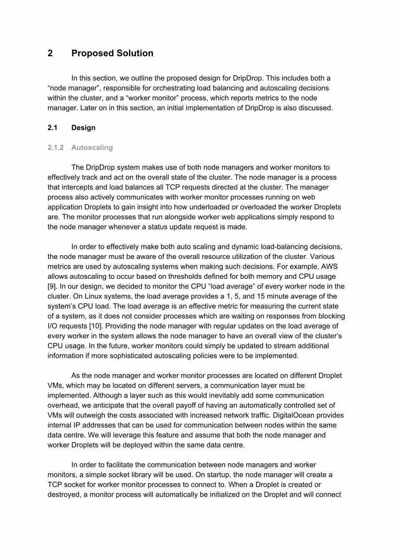
In order to effectively make both auto scaling and dynamic loadbalancing decisions, the node manager must be aware of the overall resource utilization of the cluster. Various metrics are used by autoscaling systems when making such decisions. For example, AWS allows autoscaling to occur based on thresholds defined for both memory and CPU usage [9]. In our design, we decided to monitor the CPU “load average” of every worker node in the cluster. On Linux systems, the load average provides a 1, 5, and 15 minute average of the system’s CPU load. The load average is an effective metric for measuring the current state of a system, as it does not consider processes which are waiting on responses from blocking I/O requests [10]. Providing the node manager with regular updates on the load average of every worker in the system allows the node manager to have an overall view of the cluster’s CPU usage. In the future, worker monitors could simply be updated to stream additional information if more sophisticated autoscaling policies were to be implemented.
As the node manager and worker monitor processes are located on different Droplet
VMs, which may be located on different servers, a communication layer must be implemented. Although a layer such as this would inevitably add some communication overhead, we anticipate that the overall payoff of having an automatically controlled set of VMs will outweigh the costs associated with increased network traffic. DigitalOcean provides internal IP addresses that can be used for communication between nodes within the same data centre. We will leverage this feature and assume that both the node manager and worker Droplets will be deployed within the same data centre.
In order to facilitate the communication between node managers and worker
monitors, a simple socket library will be used. On startup, the node manager will create a TCP socket for worker monitor processes to connect to. When a Droplet is created or destroyed, a monitor process will automatically be initialized on the Droplet and will connect

to the node manager process. After everytime tstatus , the node manager will send out a status update request to all worker monitors listening on the socket. The node manager will then wait at most tdeadline to get load average metrics from every worker monitor in the cluster. After receiving status updates from workers in the cluster, the node manager can aggregate the load averages of all workers within the system to get an overall view of the cluster. If a worker monitor fails to emit a response to a node manager within tdeadline , the node manager will simply aggregate the responses it received. In the initial design, it is assumed that the IP address and port of the node manager will not change. In the future, service discovery tools such as Consul [11] could be leveraged to facilitate dynamic node manager IP addresses. This could allow for worker monitor processes to easily locate an appropriate node manager Droplet on startup, regardless of what the node manager’s IP address is.
After receiving status updates from every worker monitor in the system, the node
manager will have enough data to make an informed scaling decision. At this point, the node manager may decide to horizontally scale the worker node set by adding/removing Droplets. A simple scaling policy will be configurable through the use of thresholds. By setting a minimum and maximum system load average, the node manager will be able to decide when the system is “overloaded”, and should be scaled up, and when it is “underloaded”, and should be scaled down. Through the use of DigitalOcean Droplet “snapshots”, we are able to create and save a preconfigured version of our worker nodes. If more advanced configurations are required, system provisioning tools could also be leveraged. Furthermore, we also introduce a “cooldown” time tcooldown . This is a period of time that a node manager will wait after a confirmed Droplet creation/deletion event before making any further scaling decisions. This allows the effects of any previous scaling decisions to propagate through the system and will help to prevent premature Droplet additions/deletions.
In order to automatically add/remove Droplets depending on the system load, the
DigitalOcean API must be used. Unfortunately, DigitalOcean does not provide support for “webhook” event callbacks. Third party services exist [12] which allow for requests to be sent to HTTP endpoints on the creation/deletion of DigitalOcean Droplets; however, for simplicity, we will only make use of DigitalOcean’s official API. Therefore, after the initial creation/deletion API request is made, our NodeManager must have a separate thread of execution which continuously polls DigitalOcean’s API every tpoll seconds for the Droplet’s status.
2.1.2 Dynamic Load Balancing
In addition to scaling the worker Droplet set, the node manager will also be responsible for dynamically load balancing requests between workers, based on their individual load averages. DripDrop makes use of a fairly simple dynamic version of the “weighted” round robin load balancing algorithm [13]. By calculating the “weight” of every Droplet at a regular interval tweight , the node manager is able to effectively redirect more requests to Droplets that are less overloaded (perhaps due to recently being created). A Droplet server’s “weight” is calculated by analyzing how close it is to becoming overloaded. This value is then compared to other servers in the system to figure out how many requests
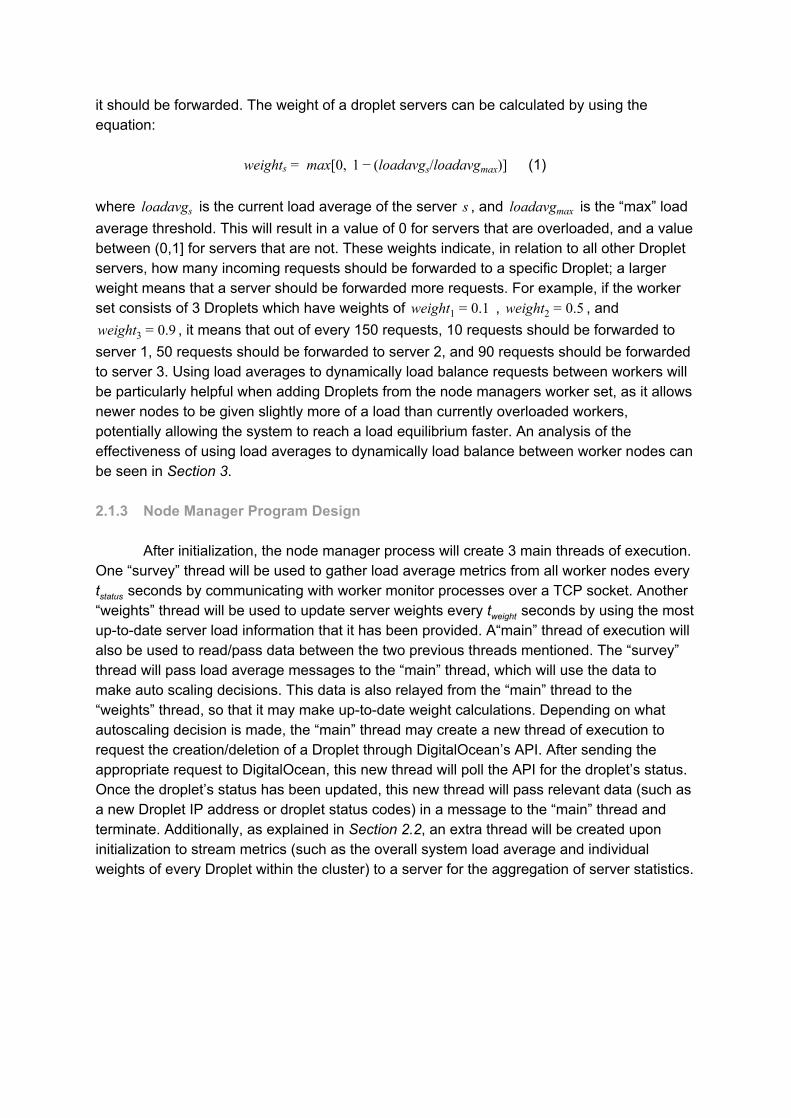
it should be forwarded. The weight of a droplet servers can be calculated by using the equation:
eight max[0, 1 loadavg /loadavg )]w s = − ( s max (1)
where is the current load average of the server , and is the “max” loadoadavgl s s oadavgl max average threshold. This will result in a value of 0 for servers that are overloaded, and a value between (0,1] for servers that are not. These weights indicate, in relation to all other Droplet servers, how many incoming requests should be forwarded to a specific Droplet; a larger weight means that a server should be forwarded more requests. For example, if the worker set consists of 3 Droplets which have weights of , , andeight .1 w 1 = 0 eight .5w 2 = 0
, it means that out of every 150 requests, 10 requests should be forwarded toeight .9w 3 = 0 server 1, 50 requests should be forwarded to server 2, and 90 requests should be forwarded to server 3. Using load averages to dynamically load balance requests between workers will be particularly helpful when adding Droplets from the node managers worker set, as it allows newer nodes to be given slightly more of a load than currently overloaded workers, potentially allowing the system to reach a load equilibrium faster. An analysis of the effectiveness of using load averages to dynamically load balance between worker nodes can be seen in Section 3.
2.1.3 Node Manager Program Design
After initialization, the node manager process will create 3 main threads of execution.
One “survey” thread will be used to gather load average metrics from all worker nodes every tstatus seconds by communicating with worker monitor processes over a TCP socket. Another “weights” thread will be used to update server weights every tweight seconds by using the most uptodate server load information that it has been provided. A“main” thread of execution will also be used to read/pass data between the two previous threads mentioned. The “survey” thread will pass load average messages to the “main” thread, which will use the data to make auto scaling decisions. This data is also relayed from the “main” thread to the “weights” thread, so that it may make uptodate weight calculations. Depending on what autoscaling decision is made, the “main” thread may create a new thread of execution to request the creation/deletion of a Droplet through DigitalOcean’s API. After sending the appropriate request to DigitalOcean, this new thread will poll the API for the droplet’s status. Once the droplet’s status has been updated, this new thread will pass relevant data (such as a new Droplet IP address or droplet status codes) in a message to the “main” thread and terminate. Additionally, as explained in Section 2.2, an extra thread will be created upon initialization to stream metrics (such as the overall system load average and individual weights of every Droplet within the cluster) to a server for the aggregation of server statistics.

2.2 Implementation 2.2.1 Node Manager
Figure 1: Node Manager design
Using the Go programming language [14] and HAProxy, we have implemented the
node manager program as described in Section 2.1.3. We decided to use Go as our programming language, because it natively provides support for simple concurrency through the use of “goroutines”, which can be regarded as “lightweight” threads, and “channels”, which allow data to be safely passed between the goroutines.
Each thread of execution described in Section 2.1.3 makes use of a single goroutine. This includes the “survey”, “weights”, “main” goroutines, as well as any goroutines created by “main” to create/destroy DigitalOcean droplets. This also includes an extra goroutine which repeatedly streams metrics to a StatsD [18] server to analyze the node manager’s performance. The node manager communicates with worker monitors to gather CPU load average metrics from each worker and dynamically load balances incoming HTTP requests based on the clusters overall load average. Additionally, depending on a set of configurable load average thresholds, the autoscaler program will use DigitalOcean’s API to add and removes worker nodes in an effort to increase QoS and save resources, respectively.
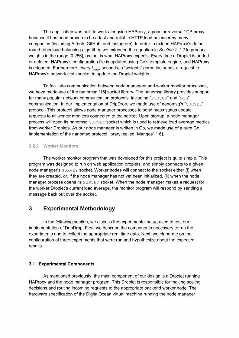
The application was built to work alongside HAProxy, a popular reverse TCP proxy, because it has been proven to be a fast and reliable HTTP load balancer by many companies (including Airbnb, GitHub, and Instagram). In order to extend HAProxy’s default round robin load balancing algorithm, we extended the equation in Section 2.1.2 to produce weights in the range [0,256], as that is what HAProxy expects. Every time a Droplet is added or deleted, HAProxy’s configuration file is updated using Go’s template engine, and HAProxy is reloaded. Furthermore, every tweight seconds, a “weights” goroutine sends a request to HAProxy’s network stats socket to update the Droplet weights.
To facilitate communication between node managers and worker monitor processes, we have made use of the nanomsg [15] socket library. The nanomsg library provides support for many popular network communication protocols, including ”PUBSUB“ and “BUS” communication. In our implementation of DripDrop, we made use of nanomsg’s “SURVEY” protocol. This protocol allows node manager processes to send mass status update requests to all worker monitors connected to the socket. Upon startup, a node manager process will open its nanomsg SURVEY socket which is used to retrieve load average metrics from worker Droplets. As our node manager is written in Go, we made use of a pure Go implementation of the nanomsg protocol library, called “Mangos” [16].
2.2.2 Worker Monitors
The worker monitor program that was developed for this project is quite simple. This
program was designed to run on web application droplets, and simply connects to a given node manager’s SURVEY socket. Worker nodes will connect to the socket either (i) when they are created, or, if the node manager has not yet been initialized, (ii) when the node manager process opens its SURVEY socket. When the node manager makes a request for the worker Droplet’s current load average, the monitor program will respond by sending a message back out over the socket. 3 Experimental Methodology
In the following section, we discuss the experimental setup used to test our implementation of DripDrop. First, we describe the components necessary to run the experiments and to collect the appropriate real time data. Next, we elaborate on the configuration of three experiments that were run and hypothesize about the expected results. 3.1 Experimental Components
As mentioned previously, the main component of our design is a Droplet running HAProxy and the node manager program. This Droplet is responsible for making scaling decisions and routing incoming requests to the appropriate backend worker node. The hardware specification of the DigitalOcean virtual machine running the node manager

application is the following: 1GB RAM, 1 CPU and a 30GB SSD disk running Ubuntu 14.04.3.
Backend worker nodes are also deployed on DigitalOcean. To simulate a real workload on the worker Droplets, a simple Python web service was developed. This application simply serves up a set of images over HTTP, and allows images to be scaled, rotated and cropped. We manually configured a virtual machine with the image processing Python program, and saved it as a DigitalOcean snapshot image. Once our autoscaler recognizes a new worker node needs to be added, a request is made to the DigitalOcean API to create a new Droplet using a snapshot image. As soon as the worker node has been created, a startup script performs the necessary configuration for the worker node to be ready for use by the node manager. The worker nodes for our experiments are running the least expensive DigitalOcean Droplet configuration with the following specifications: 512MB RAM, 1 CPU and a 20GB SSD disk running Ubuntu 14.04.3.
To simulate clients for our experiments, we use an open source load testing tool
called Locust.io [8]. Locust allows for sending mass coordinated web requests to a specific host. Our instance of Locust was configured to direct all requests to the node manager Droplet. Locust allows user behaviour “tasks” to be programmatically defined using the Python programming language. Every task is executed in a specified order by each client. For our experiment, we only assign one task to every Locust user. This task performs a simple GET request to our node manager, retrieving an image which is dynamically rotated and scaled. Locust allows for the configuration of the max number of clients, the request rate, and the rate at which clients join the load test session. We configured these parameters to simulate a steady growth of clients in our system. Once a user has joined, it executes the same task every second until a manual stop is requested.
As mentioned previously, all node managers and workers in the same data centre are able to communicate over a private network. All node manager and worker monitor process Droplets used in our experiments were located in DigitalOcean's Toronto datacentre, and were configured to communicate over a private network. Our Locust Droplet communicates with the node manager using its public IP address to simulate real response times over the WAN.
To observe and collect statistics with our experimental setup, we have the node manager Droplet utilizing a StatsD client for Go [17] to stream data to a Graphite Server. StatsD [18] is an open source network daemon that runs on Node.js. The daemon listens for statistics over UDP or TCP and sends the aggregated metrics to the Graphite backend server. Graphite[19], stores numeric timeseries data and renders graphs in real time. To host the Graphite server we use Hosted Graphite[20], a Graphite monitoring service provider. The data collected for analysis is the following:
Number of Locust requests per second Average response time per request observed by the Locust Droplet Overall load average of the cluster over time Round robin weights (per node) over time Number of worker nodes active over time
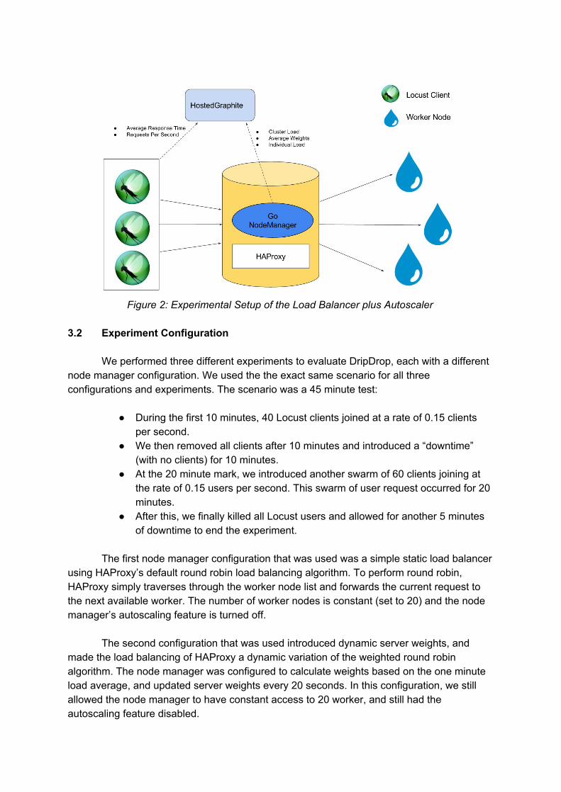
Figure 2: Experimental Setup of the Load Balancer plus Autoscaler
3.2 Experiment Configuration
We performed three different experiments to evaluate DripDrop, each with a different node manager configuration. We used the the exact same scenario for all three configurations and experiments. The scenario was a 45 minute test:
During the first 10 minutes, 40 Locust clients joined at a rate of 0.15 clients
per second. We then removed all clients after 10 minutes and introduced a “downtime”
(with no clients) for 10 minutes. At the 20 minute mark, we introduced another swarm of 60 clients joining at
the rate of 0.15 users per second. This swarm of user request occurred for 20 minutes.
After this, we finally killed all Locust users and allowed for another 5 minutes of downtime to end the experiment.
The first node manager configuration that was used was a simple static load balancer
using HAProxy’s default round robin load balancing algorithm. To perform round robin, HAProxy simply traverses through the worker node list and forwards the current request to the next available worker. The number of worker nodes is constant (set to 20) and the node manager’s autoscaling feature is turned off.
The second configuration that was used introduced dynamic server weights, and made the load balancing of HAProxy a dynamic variation of the weighted round robin algorithm. The node manager was configured to calculate weights based on the one minute load average, and updated server weights every 20 seconds. In this configuration, we still allowed the node manager to have constant access to 20 worker, and still had the autoscaling feature disabled.

The final configuration that was used introduced autoscaling in addition to dynamic
load balancing. Server weights were used in the same manner as the second experimental configuration. The experiment started with 10 worker nodes (the minimum number of workers required at all times) and the worker set was permitted to grow to a maximum of 20 workers. We configured the “overloaded” overall load average of the system to be 0.65, and the “underloaded” overall load average was set to 0.2.
We expected the second configuration to have the most optimal response time and overall load average, as it has a constant number of nodes, but is still able to dynamically balance requests between the workers. We expected the static load balancer to have the worst performance, as the simple round robin load balancing algorithm is not able to make use of system statistics when making decisions. Lastly, we expected our full DripDrop implementation to have suboptimal performance, but hoped to see a significant drop in overall resource usage, specifically during downtimes. 4 Experimental Results
In the following section, we discuss our findings after running the experiments described in Section 3. This was done by analyzing the real time data produced by StatsD and Hosted Graphite. In our analysis, we begin with the static load balancer, continue on to the dynamic load balancer, and finally analyze the performance of our fully autoscaled DripDrop implementation. The data that was analyzed is the following: overall load average for the cluster, individual worker load averages, individual server weights, response times observed by Locust clients, and the number of requests sent by Locust clients per second. In addition to these metrics, we also kept track of the number of active worker nodes when analyzing the performance of the autoscaler implementation.
4.1 Experiment 1: Static (Round Robin) Load Balancer
As mentioned previously, the first configuration that was used was a simple static, round robin load balancer with access to 20 worker nodes. As seen in Figure 3, when we started to send the first batch of requests, a spike in the overall cluster load average occurred and reached a value well above 1.0. This tells us that our cluster is overloaded. If we do an in depth analysis of each of the individual load averages within the system, we notice that the load average is not evenly distributed. As seen in Figure 4, some nodes have individual load average peaking above 2.0. This could be due to the property of the static load balancer; even though it is fair in distributing load, it does not know the overall state of the system. If a worker is hit with a slow request, the load average keeps increasing as additional processes continue to enter the run queue, causing the Droplet to become overloaded. We notice similar results when more clients are spawned over a larger time span. As seen in the latter portion of Figure 3, the load average grows to over 1.4 due to the increased number of users. In between the request attacks, when we simulate downtime, we see the load average drop to almost 0; this is as expected, as the worker nodes are not loaded at all.
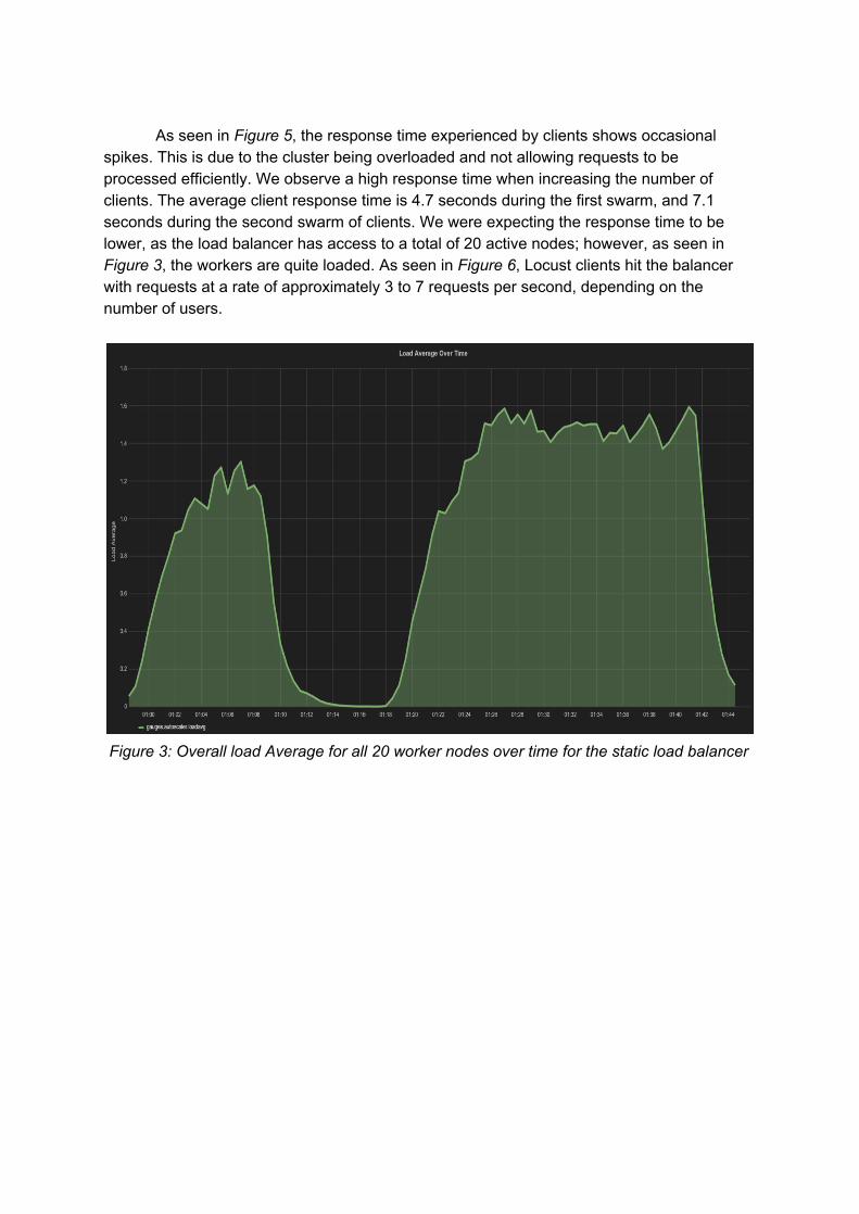
As seen in Figure 5, the response time experienced by clients shows occasional
spikes. This is due to the cluster being overloaded and not allowing requests to be processed efficiently. We observe a high response time when increasing the number of clients. The average client response time is 4.7 seconds during the first swarm, and 7.1 seconds during the second swarm of clients. We were expecting the response time to be lower, as the load balancer has access to a total of 20 active nodes; however, as seen in Figure 3, the workers are quite loaded. As seen in Figure 6, Locust clients hit the balancer with requests at a rate of approximately 3 to 7 requests per second, depending on the number of users.
Figure 3: Overall load Average for all 20 worker nodes over time for the static load balancer
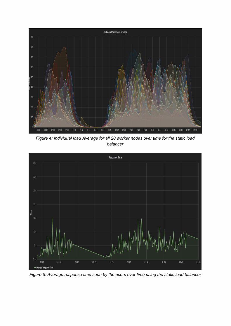
Figure 4: Individual load Average for all 20 worker nodes over time for the static load
balancer
Figure 5: Average response time seen by the users over time using the static load balancer
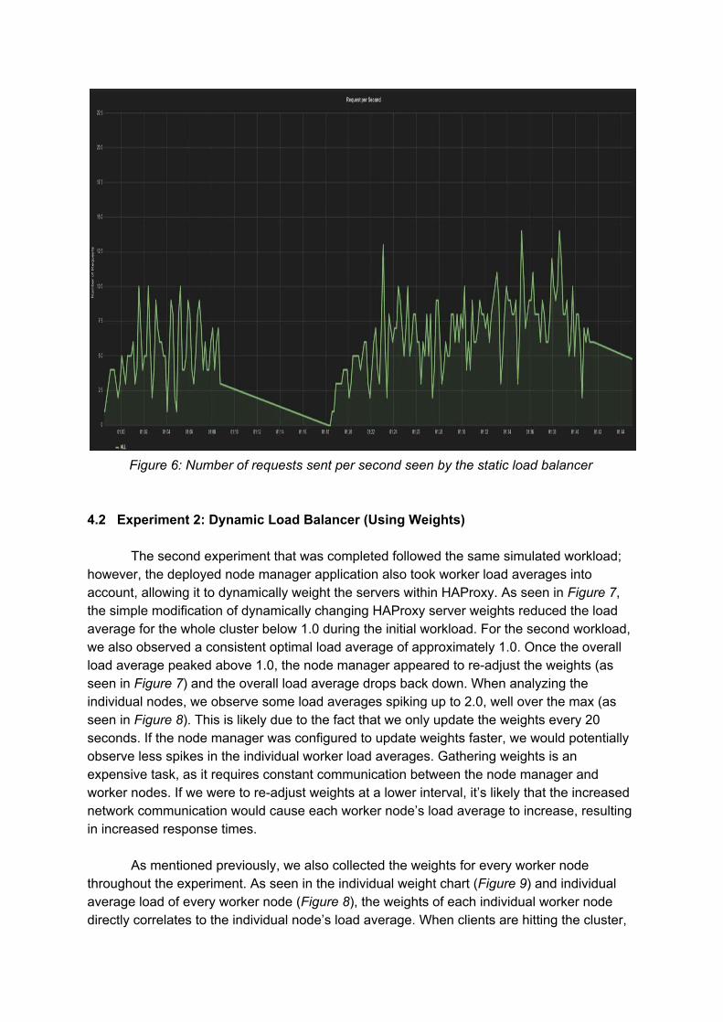
Figure 6: Number of requests sent per second seen by the static load balancer
4.2 Experiment 2: Dynamic Load Balancer (Using Weights)
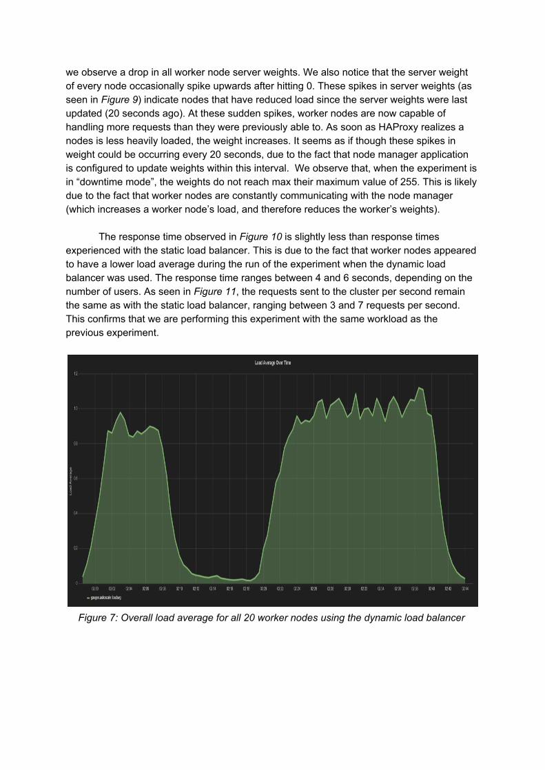
The second experiment that was completed followed the same simulated workload; however, the deployed node manager application also took worker load averages into account, allowing it to dynamically weight the servers within HAProxy. As seen in Figure 7, the simple modification of dynamically changing HAProxy server weights reduced the load average for the whole cluster below 1.0 during the initial workload. For the second workload, we also observed a consistent optimal load average of approximately 1.0. Once the overall load average peaked above 1.0, the node manager appeared to readjust the weights (as seen in Figure 7) and the overall load average drops back down. When analyzing the individual nodes, we observe some load averages spiking up to 2.0, well over the max (as seen in Figure 8). This is likely due to the fact that we only update the weights every 20 seconds. If the node manager was configured to update weights faster, we would potentially observe less spikes in the individual worker load averages. Gathering weights is an expensive task, as it requires constant communication between the node manager and worker nodes. If we were to readjust weights at a lower interval, it’s likely that the increased network communication would cause each worker node’s load average to increase, resulting in increased response times.
As mentioned previously, we also collected the weights for every worker node throughout the experiment. As seen in the individual weight chart (Figure 9) and individual average load of every worker node (Figure 8), the weights of each individual worker node directly correlates to the individual node’s load average. When clients are hitting the cluster,
we observe a drop in all worker node server weights. We also notice that the server weight of every node occasionally spike upwards after hitting 0. These spikes in server weights (as seen in Figure 9) indicate nodes that have reduced load since the server weights were last updated (20 seconds ago). At these sudden spikes, worker nodes are now capable of handling more requests than they were previously able to. As soon as HAProxy realizes a nodes is less heavily loaded, the weight increases. It seems as if though these spikes in weight could be occurring every 20 seconds, due to the fact that node manager application is configured to update weights within this interval. We observe that, when the experiment is in “downtime mode”, the weights do not reach max their maximum value of 255. This is likely due to the fact that worker nodes are constantly communicating with the node manager (which increases a worker node’s load, and therefore reduces the worker’s weights).
The response time observed in Figure 10 is slightly less than response times experienced with the static load balancer. This is due to the fact that worker nodes appeared to have a lower load average during the run of the experiment when the dynamic load balancer was used. The response time ranges between 4 and 6 seconds, depending on the number of users. As seen in Figure 11, the requests sent to the cluster per second remain the same as with the static load balancer, ranging between 3 and 7 requests per second. This confirms that we are performing this experiment with the same workload as the previous experiment.
Figure 7: Overall load average for all 20 worker nodes using the dynamic load balancer
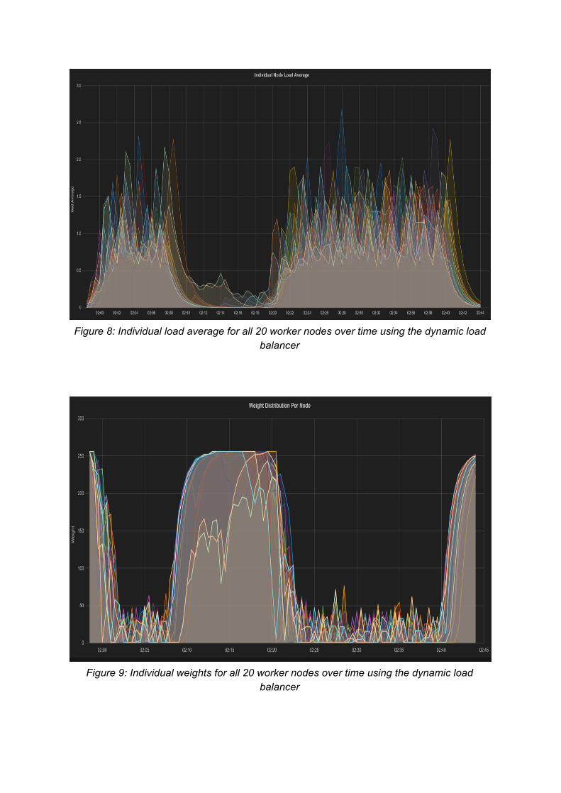
Figure 8: Individual load average for all 20 worker nodes over time using the dynamic load
balancer
Figure 9: Individual weights for all 20 worker nodes over time using the dynamic load
balancer
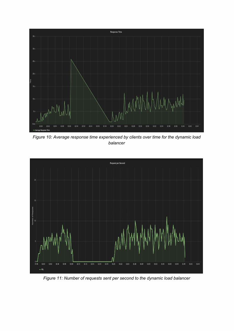
Figure 10: Average response time experienced by clients over time for the dynamic load
balancer
Figure 11: Number of requests sent per second to the dynamic load balancer
4.3 Experiment 3: Dynamic Load Balancer and Autoscaler (DripDrop)
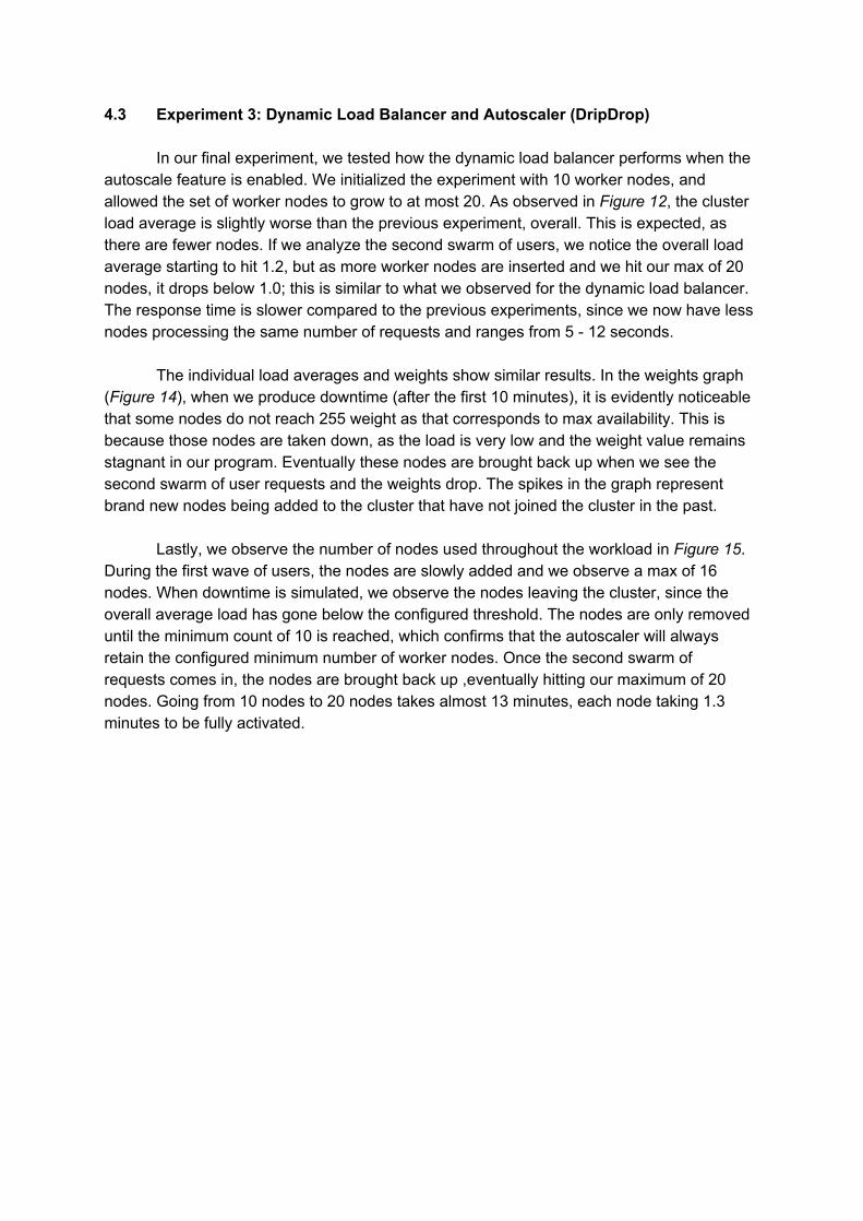
In our final experiment, we tested how the dynamic load balancer performs when the autoscale feature is enabled. We initialized the experiment with 10 worker nodes, and allowed the set of worker nodes to grow to at most 20. As observed in Figure 12, the cluster load average is slightly worse than the previous experiment, overall. This is expected, as there are fewer nodes. If we analyze the second swarm of users, we notice the overall load average starting to hit 1.2, but as more worker nodes are inserted and we hit our max of 20 nodes, it drops below 1.0; this is similar to what we observed for the dynamic load balancer. The response time is slower compared to the previous experiments, since we now have less nodes processing the same number of requests and ranges from 5 12 seconds.
The individual load averages and weights show similar results. In the weights graph
(Figure 14), when we produce downtime (after the first 10 minutes), it is evidently noticeable that some nodes do not reach 255 weight as that corresponds to max availability. This is because those nodes are taken down, as the load is very low and the weight value remains stagnant in our program. Eventually these nodes are brought back up when we see the second swarm of user requests and the weights drop. The spikes in the graph represent brand new nodes being added to the cluster that have not joined the cluster in the past.
Lastly, we observe the number of nodes used throughout the workload in Figure 15.
During the first wave of users, the nodes are slowly added and we observe a max of 16 nodes. When downtime is simulated, we observe the nodes leaving the cluster, since the overall average load has gone below the configured threshold. The nodes are only removed until the minimum count of 10 is reached, which confirms that the autoscaler will always retain the configured minimum number of worker nodes. Once the second swarm of requests comes in, the nodes are brought back up ,eventually hitting our maximum of 20 nodes. Going from 10 nodes to 20 nodes takes almost 13 minutes, each node taking 1.3 minutes to be fully activated.
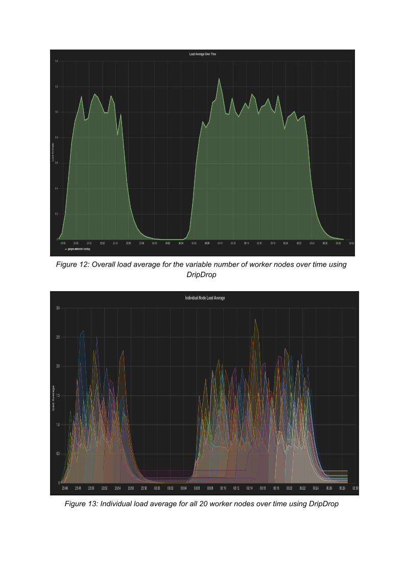
Figure 12: Overall load average for the variable number of worker nodes over time using
DripDrop
Figure 13: Individual load average for all 20 worker nodes over time using DripDrop
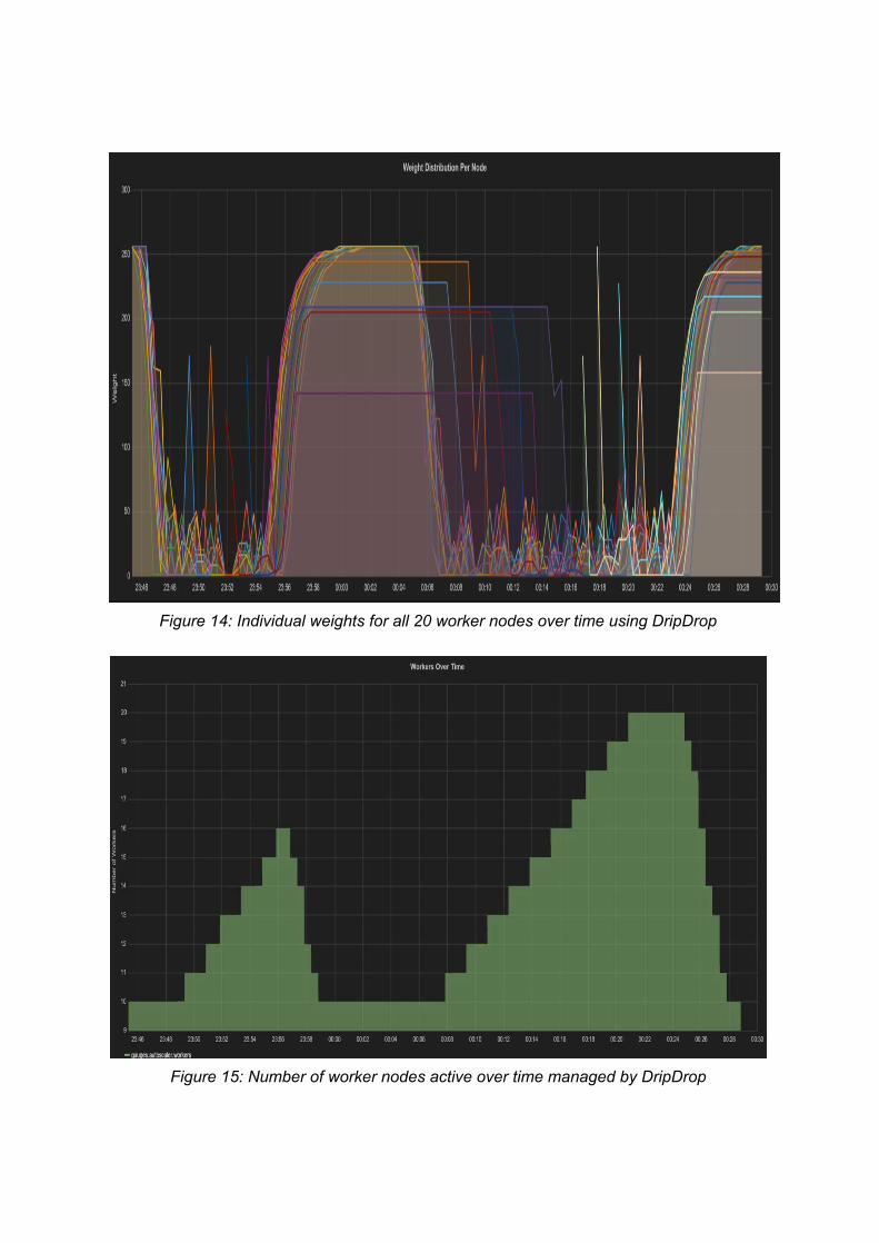
Figure 14: Individual weights for all 20 worker nodes over time using DripDrop
Figure 15: Number of worker nodes active over time managed by DripDrop
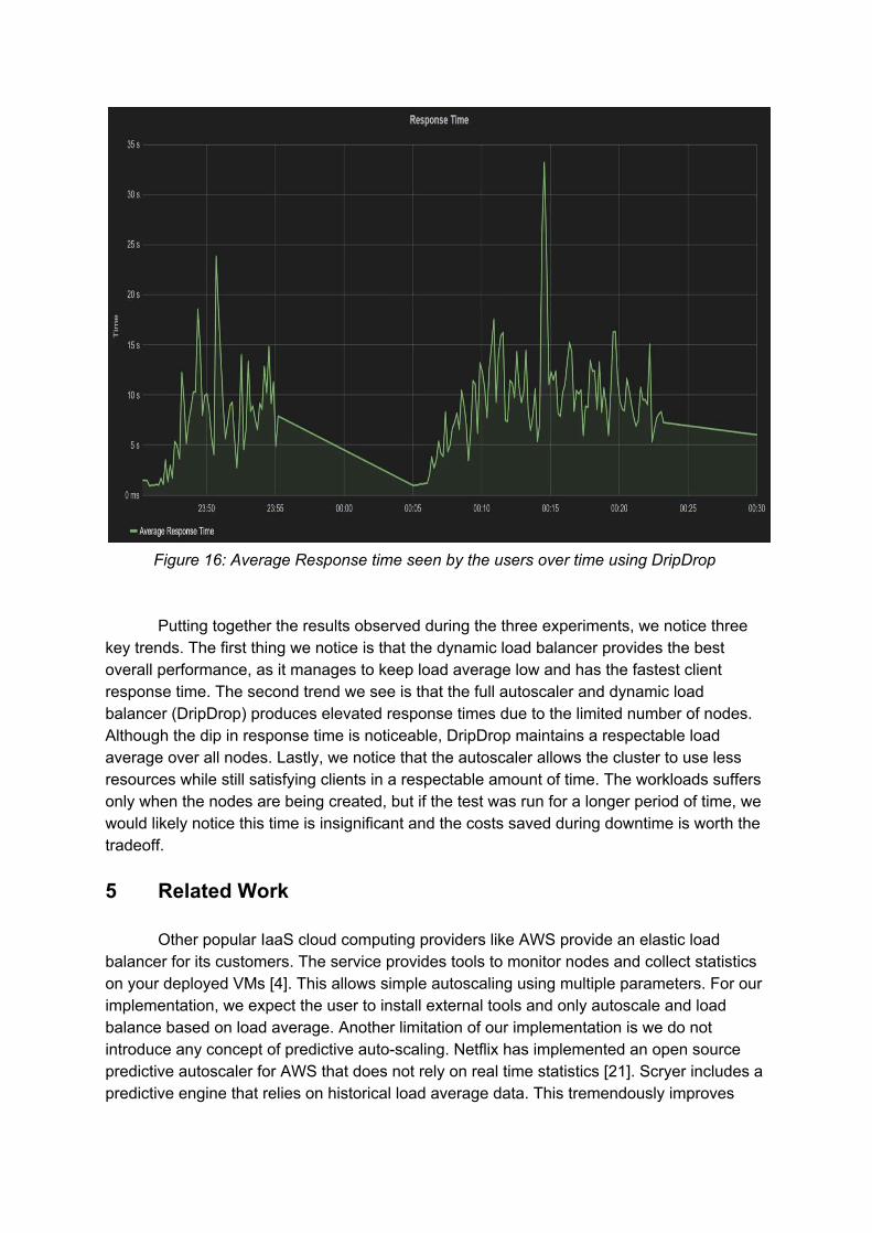
Figure 16: Average Response time seen by the users over time using DripDrop
Putting together the results observed during the three experiments, we notice three key trends. The first thing we notice is that the dynamic load balancer provides the best overall performance, as it manages to keep load average low and has the fastest client response time. The second trend we see is that the full autoscaler and dynamic load balancer (DripDrop) produces elevated response times due to the limited number of nodes. Although the dip in response time is noticeable, DripDrop maintains a respectable load average over all nodes. Lastly, we notice that the autoscaler allows the cluster to use less resources while still satisfying clients in a respectable amount of time. The workloads suffers only when the nodes are being created, but if the test was run for a longer period of time, we would likely notice this time is insignificant and the costs saved during downtime is worth the tradeoff. 5 Related Work
Other popular IaaS cloud computing providers like AWS provide an elastic load balancer for its customers. The service provides tools to monitor nodes and collect statistics on your deployed VMs [4]. This allows simple autoscaling using multiple parameters. For our implementation, we expect the user to install external tools and only autoscale and load balance based on load average. Another limitation of our implementation is we do not introduce any concept of predictive autoscaling. Netflix has implemented an open source predictive autoscaler for AWS that does not rely on real time statistics [21]. Scryer includes a predictive engine that relies on historical load average data. This tremendously improves

performance, since the AWS instances are ready before the high period of workload hits the server. In our implementation we notice a considerably high response time when nodes in the backend are in the process of scaling up.
Resource provisioning and load balancing has been a popular research topic and many related papers have been published relating to techniques and analysis of autoscaling in a VM cluster. One of the papers, titled “Autoscaling Web Applications in Heterogeneous Cloud Infrastructures”, researches different scaling parameters dependent on workload and cloud infrastructure [2]. One of the techniques they mention is based on load average. The potential next steps for our project would be to analyze various kind of workloads and use different cluster statistics to balance load, instead of simply using load average. Fernandez et al. experiment with highly variable workloads and provision resources based on load average and customer demand. This is similar to our approach, but they prioritize based on the type of user and request. Since we only tested our system with one type of user, we did not implement prioritization between requests. 6 Conclusion
With a simple API provided by DigitalOcean, the ability to create snapshots of worker nodes, and a configurable load balancer (HAProxy), we have all the tools necessary to implement a dynamic load balancer and autoscaler for DigitalOcean. The implemented autoscaler, DripDrop, allows for easy scaling of worker Droplets. Furthermore, the dynamic load balancer bases routing decisions on the clusters load average, allowing for intelligent load balancing. In our experiments, we compare our implementation with a standalone static and dynamic load balancer, both using HAProxy. We aimed to implement an autoscaler that was capable of minimizing resource usage by dynamically adding and removing Droplets. The tradeoff is slower response time, but the cost tradeoff is worth it (specifically if the workload runs for a long period).
We found that the creation of new worker nodes is a slow process and can be
drastically improved if we could predict when we would have high load durations during a workload. The performance is highly dependent on the configuration of the autoscaler and load balancer. The maximum load average threshold (when the autoscaler decides to add a worker node) is highly dependant on the workload. The savings in cost are only evident when a long running workload is utilizing a large number of workers nodes. In addition, our node manager currently represents a single point of failure in our design. HAProxy supports slave load balancers which run dormant until the master has failed; this could be explored in the future.
Since the autoscaler increases response time due to the limited number of nodes, we
believe this autoscaler implementation is more appropriate for noncritical applications that can be tolerant to potential dips in response time. Monitoring load average for individual workers is an expensive operation and contributes to the increasing load average. Theoretically, the node manager itself should be able to estimate the load of a worker node based on the number of requests it has sent that node. Lastly, we realized we cannot fully
optimize cost during downtime. Since the time to add a node is slow, we may want to revise the design to keep a minimum number of nodes active during busy workload periods, otherwise our performance struggles significantly.
The technique to analyze the load of a cluster is not new, but has not been tested on
DigitalOcean Droplet clusters. Since a big component of our project is using a configurable version of HAProxy, we believe our design can be extended towards other infrastructure as a service (IaaS) cloud computing platforms that currently have limited support for dynamic load balancing and autoscaling. References [1] DigitalOcean: Simple Cloud Infrastructure for Developers. December 20, 2015,
<https://www.digitalocean.com/> 2012 [2] Fernandez, H., Pierre, G., & Kielmann, T. (2014). Autoscaling Web applications in
heterogeneous cloud infrastructures. Cloud Engineering (IC2E), 2014 IEEE International Conference on. IEEE.
[3] Understanding the Cloud Computing Stack: SaaS, PaaS, IaaS. December 20, 2015,
<http://www.rackspace.com/> 2011 [4] AWS | Elastic Load Balancing Cloud Network Load Balancer. December 21, 2015,
<https://aws.amazon.com/elasticloadbalancing/> 2009 [5] Rackspace Cloud Auto Scale. December 19, 2015,
<http://www.rackspace.com/cloud/autoscale> 2013 [6] HAProxy. October 16, 2015, <http://www.haproxy.org/> 2009 [7] nginx. October 16, 2015, <http://nginx.org/en/> 2009 [8] Locust A modern load testing framework. December 21, 2015,< http://locust.io/> 2014 [9] The Netflix Tech Blog: Auto Scaling in the Amazon Cloud. December 23, 2015,
<http://techblog.netflix.com/2012/01/autoscalinginamazoncloud.html> 2012 [10] Examining Load Average | Linux Journal. December 23, 2015,
<http://www.linuxjournal.com/article/9001> 2006 [11] Consul by HashiCorp. December 23, 2015, <https://www.consul.io/> 2014 [12] Digital Ocean & Webhooks by Zapier Integrations December 23, 2015,
<https://zapier.com/zapbook/digitalocean/webhook/> 2013 [13] Katevenis, M., Sidiropoulos, S., & Courcoubetis, C. (1991). Weighted roundrobin cell
multiplexing in a generalpurpose ATM switch chip. Selected Areas in Communications, IEEE Journal on, 9(8), 12651279.
[14] The Go Programming Language. October 16, 2015,< https://golang.org/> 2011 [15] nanomsg. December 23, 2015, <http://nanomsg.org/> 2012 [16] gomangos/mangos ∙ GitHub. December 24, 2015, <https://github.com/gdamore/mangos>
2014 [17] cactus/gostatsdclient ∙ GitHub. December 21, 2015
<https://github.com/cactus/gostatsdclient> 2012 [18] etsy/statsd ∙ GitHub. December 21, 2015 <https://github.com/etsy/statsd >2010 [19] "Graphite Scalable Realtime Graphing Graphite.". December 21 2015
<http://graphite.wikidot.com/> 2008 [20] "Hosted Graphite Graphite as a service" December 21 2015
<https://www.hostedgraphite.com/> 2012 [21] "Scryer: Netflix's Predictive Auto Scaling Engine " December 22, 2015
<http://techblog.netflix.com/2013/11/scryernetflixspredictiveautoscaling.html> 2013