Embed Size (px)
Citation preview
Driver and Sensor Node SelectionStrategies Optimizing the
Controllability Properties of ComplexDynamical Networks
Ph.D Thesis
Francesco Lo Iudice
Tutor
Ch.mo Prof. Franco Garofalo
University of Naples Federico II
Department of Electrical Engineering and Information Technology
Naples, Italy
2016

Contents
1 Introduction 1
1.1 Thesis outline . . . . . . . . . . . . . . . . . . . . . . . . . . . . . . . . . . . 3
2 Background 5
2.1 Complex networks . . . . . . . . . . . . . . . . . . . . . . . . . . . . . . . . 5
2.2 The structure of complex networks: algebraic graph theory . . . . . . . . . . 6
2.3 Networks of Linear Dynamical systems . . . . . . . . . . . . . . . . . . . . . 8
2.4 Controllability of Linear Dynamical Systems . . . . . . . . . . . . . . . . . . 9
2.4.1 Structural Controllability of Linear Dynamical Systems . . . . . . . . 9
2.5 Controllability of Complex Networks . . . . . . . . . . . . . . . . . . . . . . 10
3 Partial Controllability of Complex Networks 13
3.1 Problem Formulation . . . . . . . . . . . . . . . . . . . . . . . . . . . . . . . 16
3.2 Problem Solution . . . . . . . . . . . . . . . . . . . . . . . . . . . . . . . . . 18
3.3 Computational Considerations . . . . . . . . . . . . . . . . . . . . . . . . . . 24
4 Structural Permeability of Complex Networks to Control Signals 31
4.1 Permeability analysis of real network topologies . . . . . . . . . . . . . . . . 33
5 Heuristic Driver Node Selection Strategies 45
5.1 Performance Evaluation of Heuristic Strategy 2 . . . . . . . . . . . . . . . . 55
6 Partial Observability of Complex Networks 61
6.1 Observability of Dynamical Systems . . . . . . . . . . . . . . . . . . . . . . . 61
6.2 Sensor Node Selection Strategies . . . . . . . . . . . . . . . . . . . . . . . . . 62
6.3 Computational Considerations . . . . . . . . . . . . . . . . . . . . . . . . . . 68

ii Contents
7 Conclusions 70
7.1 Open problems and Future Work . . . . . . . . . . . . . . . . . . . . . . . . 71
Bibliography 72

List of Figures
2-1 An example of a dilation, node t1 and t2 compose the set T while node s is
the only node having an edge exiting it and entering the nodes of T . . . . . . 7
2-2 (a) The graph of a simple network (b) Its maximal matching. (c) The orange
node is the only driver node selected by the maximal matching. (d) The red
nodes are the driver nodes required to ensure complete controllability of this
simple network according to definiton 2.5.1. . . . . . . . . . . . . . . . . . . 12
3-1 A very simple controlled network. The orange arrow indicates that the input
u is injected in node 1 which is thus the only driver node. . . . . . . . . . . . 14
3-2 Plot of three different controllable subspaces corresponding to three different
sets of values of the free entries of the pair (F,B) for the controlled network
portrayed in Fig. 3-1. . . . . . . . . . . . . . . . . . . . . . . . . . . . . . . 15
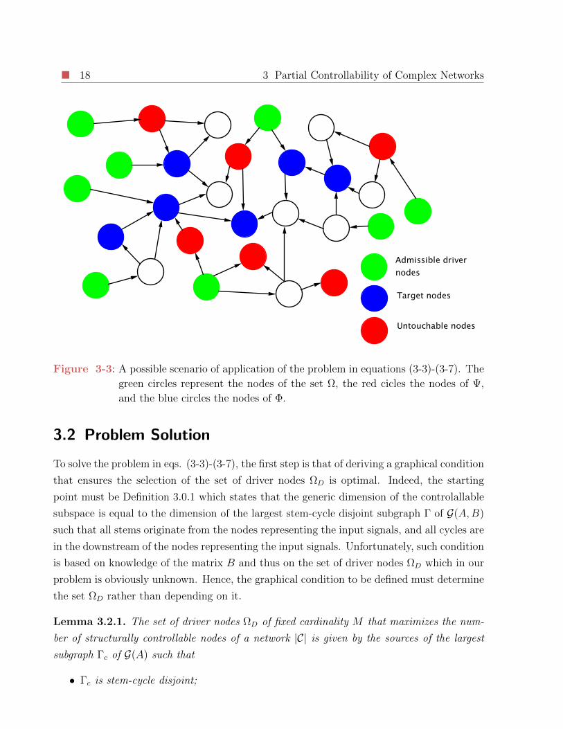
3-3 A possible scenario of application of the problem in equations (3-3)-(3-7). The
green circles represent the nodes of the set Ω, the red cicles the nodes of Ψ,
and the blue circles the nodes of Φ. . . . . . . . . . . . . . . . . . . . . . . . 18
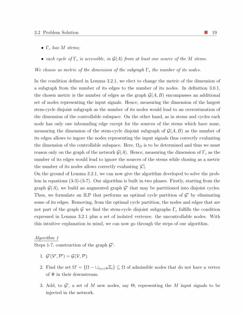
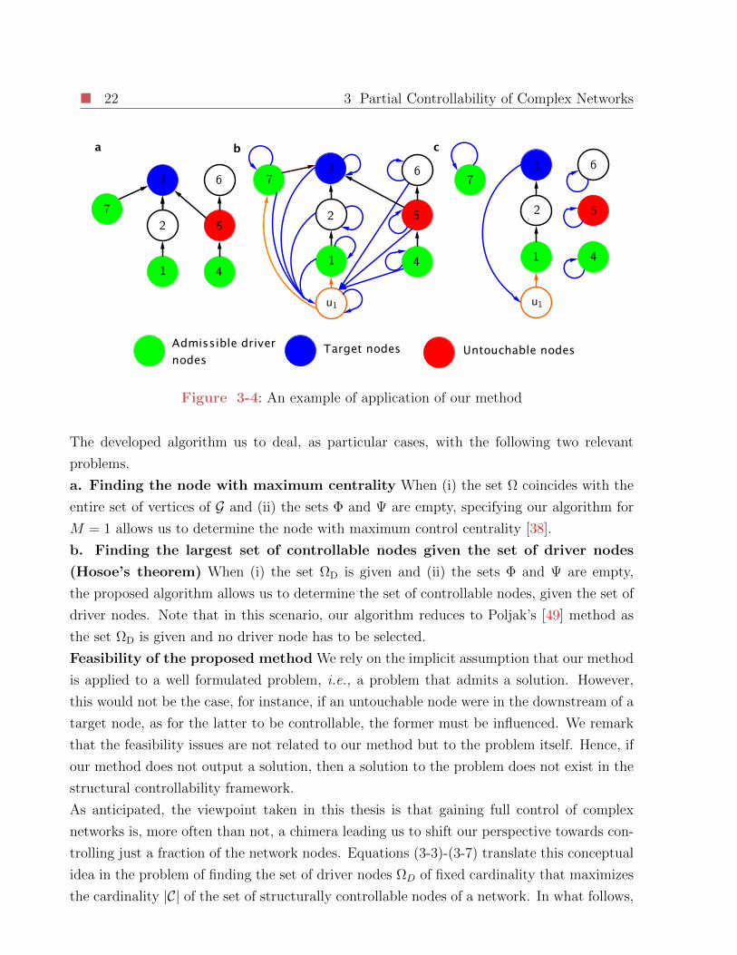
3-4 An example of application of our method . . . . . . . . . . . . . . . . . . . . 22
4-1 Plot of the sequence |C(M)| for the Budding Yeast Protein Structure network
(blue) and the SciNet citation network (red). Both |C(M)| and M are nor-
malized by dividing them by number of nodes of the two networks to allow
comparing the results on the same scale. . . . . . . . . . . . . . . . . . . . . 33
4-2 Plot of the network permeability µ over the network average degree 〈k〉 for
29 real network topologies. The black dashed line represents the least square
regression line of the data. . . . . . . . . . . . . . . . . . . . . . . . . . . . . 34
4-3 Plot of the network permeability µ over the parameter β for 30 real network
topologies. The black dashed line represents the least square regression line
of the data. . . . . . . . . . . . . . . . . . . . . . . . . . . . . . . . . . . . . 35

iv List of Figures
4-4 Plot of the loss of permeability ∆µ(Ψ) over the parameter β when a we have
that |Ψ| = 0.05N and b we have that |Ψ| = 0.10N . . . . . . . . . . . . . . . 38
4-5 Plot of the loss of permeability ∆µ(Ψ) over the parameter β. The title of each
panel corresponds to the criterion with which the set of untouchable nodes
responsible of the loss of permeability was selected. . . . . . . . . . . . . . . 40
4-6 (a) Plot of the outdegree (green) and indegree(magenta) of the optimal driver
nodes. (b) Plot of the average degree of the nodes of C (green) and of the
nodes of C (magenta) over M . Then former exhibit higher degree than the
latter. . . . . . . . . . . . . . . . . . . . . . . . . . . . . . . . . . . . . . . . 41
4-7 Plot of the relation between the network permeability µ and the maximum
centrality |C(1)| of its nodes. . . . . . . . . . . . . . . . . . . . . . . . . . . . 43
5-1 (a) The graph of a model network. (b) the DAG condensation of the model
network. (b) The two-level reduced graph. Red circles represent RSCCs ri
such that |∆(ri)| 6= 0, the blue circles represent SCCs si such that |si| > 0.
(d) Green circles represent the nodes selected as drivers while yellow circles
represent the nodes accessible from the drivers. The blue circles represent the
nodes that are inaccessible from the drivers. . . . . . . . . . . . . . . . . . . 53
5-2 Plot of the fraction of the network nodes that can be made controllable over
the number of driver nodes deployed M according to Algorithm 1 (blue) and
Heuristic Strategy 2 (yellow) for the Cora citation network. . . . . . . . . . . 57
5-3 Plot of the fraction of the network nodes that can be made controllable over
the number of driver nodes deployed M according to Algorithm 1 (blue) and
Heuristic Strategy 2 (yellow) for the Twitter Lists network. . . . . . . . . . . 58
5-4 Plot of the fraction of the network nodes that can be made controllable over
the number of driver nodes deployed M according to Algorithm 1 (blue) and
Heuristic Strategy 2 (yellow) for (a) the DBLP citation network and (b) the
B-cell Interactome Network. . . . . . . . . . . . . . . . . . . . . . . . . . . 59
6-1 Graph of the dual representation of a very simple observed network. . . . . . 63
6-2 Plot of three different observable subspaces corresponding to three different
sets of values of the free entries of the pair (F T , CT ) for the controlled network
portrayed in Fig. 3-1. . . . . . . . . . . . . . . . . . . . . . . . . . . . . . . 64

List of Tables
4-1 List of real network topologies analysed. . . . . . . . . . . . . . . . . . . . . 36
5-1 Main topological features of the Cora citation Network . . . . . . . . . . . . 55
5-2 Main topological features of the Twitter Lists Network . . . . . . . . . . . . 56
5-3 Main topological features of the B-cell interactome and DBLP citation networks 59
v
Abstract
In recent years, complex networks have attracted the attention of researchers throughout the
fields of science due to their ubiquity in natural and artificial settings. While the spontaneous
emergence of collective behavior has been thoroughly studied, and has inspired researchers
in the design of control strategies able to reproduce it in artificial scenarios, our ability to
arbitrarily affect the behavior of complex networks is still limited. To start filling this void,
in the past five years, researchers have focused on the preliminary condition of selecting
the nodes where input signals have to be injected so to ensure complete controllability of
complex networks. Unfortunately, the scale of complex networks is such that more often than
not too many input signals are required to arbitrarily modify the behavior of all the nodes
of a network. Departing from the idea that achieving complete controllability of complex
networks is a chimera, in this thesis, we present a comprehensive toolbox of input selection
algorithms so to ensure controllability of the largest number of nodes of a network. Then,
we complement this toolbox with algorithms for sensor placement so to also guarantee, when
possible, observability of these nodes, thus allowing the implementation of feedback control
strategies. Finally, an outlook on input selection strategies so to allow controlling a set of
nodes of a network with reasonable energy is provided.
CHAPTER 1
Introduction
Abstract models of real world phenomena have been of paramount importance throughout
the fields of science. The development of these mathematical representations has been mostly
delegated to researchers of the physics community, as natural phenomena have been the
main objects to be described. Some of these representations, such as Newton’s three laws of
motion, Maxwell’s equations on electromagnetism, and Einstein’s field equations have the
character of theories due two their general validity. These have constituted the basis for
the development of nearly an infinite number of laws and have constituted the anchor for
countless real and numerical experiments.
In recent years, the enormous advances mankind has made in its comprehension of physical
phenomena have brought more and more researchers to study real world systems such as
power grids [10, 1], fish schools and other biological networks [53], financial markets [41], or
social networks [57]. These systems cannot be described by separately modeling each of their
components and ignoring their interactions as the latter play a crucial role in determining
the overall system behavior. In fact, one could argue that a mathematical model of several
of these systems cannot be formulated as some of their components to not obey to purely
physical laws. Nevertheless, developing abstract representations able to capture some key
aspects of their behavior can be critical [54, 11, 12, 8]. To do so, researchers have comple-
mented methods of the physics community with tools from dynamical systems and graph
theory, thus developing a new discipline, Networks Science, a paradigm for the interpretation
and the description of the behavior of real world complex systems.
At first, the complex network paradigm has been mainly used as a tool for modeling the
emergence of collective behavior in natural settings [2, 43, 47]. The laws that proved suc-
cessful in capturing phenomena observed in nature have then inspired the design of control
strategies able to reproduce these phenomena in artificial settings [58, 6, 65]. Prominent
2 1 Introduction
examples are the numerous consensus protocols deployed for controlling the formation of
fleets of autonomous vehicles [50, 52, 51, 9]. More recently, the use of the complex network
paradigm has been extended to describe systems that do not exhibit emerging collective
behaviors, but where modeling the interactions between the systems’ components is critical
in order to capture their main features. Skipping through the recent literature, we observe
that financial systems, gene-regulatory networks, social networks, food webs and electronic
circuits are frequently modeled as complex dynamical networks although they do not nec-
essarily exhibit collective behaviors [31, 26, 8, 33, 57]. Consistently, from now on the term
Complex Network will be used without specifying if it is referred to the real system or its
mathematical abstraction, unless the contexts requires doing so.
Given the success that the complex network paradigm has had in describing the behavior
of very diverse real world systems, it has been proposed as a testbed for control strategies
aiming at affecting the behavior of these systems. From a theoretical perspective, the goal
of being able to tame these complex networks has posed the following question: what are
the conditions to be fulfilled in order to guarantee being able to arbitrarily affecting the
behavior of a network? To answer this question, researchers have started by studying the
following general problem: which nodes of a complex network must be directly controlled
in order to be able to arbitrarily modify the behavior of the entire network? This problem
has been widely studied in the recent literature and different metrics have been proposed for
the optimal selection of the nodes to be directly controlled. Nevertheless, most of the recent
literature has focused on gaining full control of the network behavior [37, 66, 61]. Here,
we depart from the opposite perspective, as our point of view is that complex networks are
perhaps too complex (!) to be fully controlled. This can be due to economic constraints
limiting the number of nodes where input signals must be injected or to physical reasons, as
the nodes that should be directly controlled in order to be able to affect the behavior of the
whole network are inaccessible.
This shift of perspective from the ambition of completely controlling the behavior of complex
networks to the more realistic goal of controlling only a fraction of the network nodes brings
us to address two classes of problems. Firstly, we ask ourselves in which nodes shall we
inject input signals so to maximize our ability to control the network behavior? Secondly,
we face the problem of selecting the nodes where sensors should be placed so to be able to
reconstruct the state of the nodes we are able to control.
Developing a toolbox of algorithms for the selection of the nodes where input signals must
be injected so to maximize our ability to affect the network behavior allows us to break new
ground in the analysis of the relation between the network structure and its readiness to
1.1 Thesis outline 3
be made controllable. Our analyses ultimately lead us to define the network permeability
to control signals, a measure of the propensity of a network to be made controllable. By
analyzing the permeability of several real and model networks, we find that this index is
strongly influenced by the networks structure. As a byproduct, we also find that both the
nodes where input signals must be injected in order to maximize our ability to control a
network and the nodes that are easily made controllable are characterized by structural
signatures. Altogether, our findings provide the reader with a toolbox of algorithms for the
selection of the nodes where input signals and sensors must be placed in complex dynamical
networks together with a characterization of the structural properties that determine the
network permeability and the ease with which the network nodes can be controlled.
1.1 Thesis outline
In Chapter 2 we introduce the general mathematical model of a complex dynamical network.
Then, we introduce some notatation and mathematical preliminaries, mostly focusing on the
graph-theoretic tools we will leverage to give our results. As we will study controllability of
a specific class of complex networks, those that exhibit linear node dynamics, we intoduce
the concept of controllability of linear systems and illustrate the theory of structural con-
trollability. Finally, we illustrate how this theory can be leveraged to study controllability
of complex dynamical networks.
After having given, in Chapter 2, all the theoretical background necessary to study controlla-
bility of complex networks, in Chapter 3, we introduce the concept of partial controllability
of complex networks, which we define as the problem of selecting the nodes where input
signals must be injected in order to maximize the number of nodes of the network that
can be made controllable. Then, we give an algorithm able to solve this problem by first
translating it into a graph optimization problem and then into an ILP. Finally, a discussion
of the computational complexity of the ILP is given to end the chapter.
In Chapter 4, the tools developed in Chapter 3 are leveraged to uncover the ease with
which complex networks can be made controllable regardless of the number of input signals
deployed for the task. To measure the readiness with which a complex network can be made
controllable, we introduce the network permeability to control signals, and we discover that
this index is strongly tied to the network structure. We aslo find that the nodes where
input signals must be injected in order to maximize our ability to control a network are
characterized by structural signatures.

4 1 Introduction
In Chapter 5, we exploit the results of the numerical analysis performed in 4 to develop heuris-
tic driver node selection strategies with lower computational complexity than the strategy
introduced in Chapter 3. In Chapter 6, we give an algorithm capable of solving the problem
of placing a set of sensors in a subset of the network nodes in order to guarantee observ-
ability of the controllable nodes of a network. The aim of this Chapter is to complement
the algorithms provided in Chapters 3 and 5 with sensor node selection strategies in order
to allow deploying feedback control strategies for complex dynamical networks. Finally, in
Chapter 7 Conclusions are drawn and an outlook is given on the current topics that are being
investigated by the researchers working on controllability and control of complex dynamical
networks.
The results given in Chapters 3 and 4 have been presented in ref. [40], while two papers
presenting the results in Chapters 5 and 6 are under currently submission.
CHAPTER 2
Background
2.1 Complex networks
The complex network paradigm allows to model real world complex systems as an ensemble
of dynamical systems, the nodes, interacting among each other according to an underlying
topology. The general form of the equation describing the dynamics of the i-th of N network
nodes is
xi = fi(xi) +∑j 6=i
aijhij(xi, xj) (2-1)
where xi is the state of the i-th node of the network, fi(xi) is the vector field describing its
intrinsic dynamics, and hij(xi, xj) is the function that defines the interaction between node
i and node j. The binary coefficient aij indicates whether the dynamics of node i are, or are
not, dependent on that of node j.
From a purely mathematical perspective, considering equation (2-1) for all the network nodes
is sufficient to understand the network behavior, as is the case for all dynamical systems.
Nevertheless directly approaching the dynamic equations of a network often proves unfeasible
and not necessary. With some assumptions on the intrinsic node dynamics, several properties
of complex networks can be studied by only taking into account the network topology and
this, perhaps, is the main feature of the complex network paradigm. As this is the approach
taken in this thesis, in the following section we introduce the graph theoretical tools necessary
to cope with the topology of complex networks.

6 2 Background
2.2 The structure of complex networks: algebraic graph
theory
Rewriting eq. (2-1) for all the network nodes in compact form, we obtain the equation
x = F (x) + AH(x), (2-2)
where the matrix A = aij is the adjacency matrix that defines the topology of the network,
that is, a graph G(V ,P) where V = v1, v2, . . . vN is the set of the N network nodes and
P ⊂ V × V is the set of network edges. In the graph G there is an edge pij connecting node
vj to node vi if the corresponding binary element aij of the adjacency matrix A takes the
value of 1. We can distinguish between two general categories of adjacency matrices which
allow defining two general classes of graphs:
Definition 2.2.1. A graph G is said to be undirected if its adjacency matrix is symmetric.
In such case, the existence of the edge pij directly implies the existence of the edge pji.
Definition 2.2.2. A graph G is said to be directed (or a digraph) if its adjacency matrix is
not symmetric.
In this thesis, we will mainly focus on the general case of digraphs and, in some cases, show
how some results simplify in the case of undirected network garphs. As we rely on struc-
tural controllability theory, we make use of the following definitions of elementary digraph
structures [36]:
Definition 2.2.3. A stem is an elementary path, i.e., a sequence of oriented edges (pij), (pjk), ..., (plm)such that i 6= m. We will name the start node vi a source, and the end node vm a sink.
Definition 2.2.4. A cycle is an an elementary path that starts and ends in the same node.
Definition 2.2.5. We say that vj is accessible from vi if there exists a directed path from vi
to vj and that in such a case vi is in the upstream of vj.
Definition 2.2.6. We say that a subgraph Γ of a graph G is stem-cycle disjoint if it is
composed of an arbitrary number of stems and cycles that do not share any node nor edge.
Moreover, we will make use of the following graph-theoretic definitions.
Definition 2.2.7. A strongly connected component (SCC) of a graph G, is a subgraph such
that ∀vi, vj ∈ SCC there exists a path from node vi to node vj.

2.2 The structure of complex networks: algebraic graph theory 7
Definition 2.2.8. A root strongly connected component (RSCC) of a graph G is an SCC
ri of G such that there are no edges entering a node of ri that exit from a node that is not
encompassed in ri.
Definition 2.2.9. A Directed Acyclic Graph (DAG) is a graph that does not encompass
cycles.
Definition 2.2.10. A digraph G(V ,P) contains a dilation iff there exists a set T ⊂ V that
does not include source nodes, such that the number of elements in T is larger than the
number of nodes having edges exiting them and entering the nodes in the set T . An example
of a dilation is shown in Figure 2-1.
Definition 2.2.11. The indegree kin of node vi is equal to the number of edges entering node
vi.
Definition 2.2.12. The outdegree kout of node vi is equal to the number of edges exiting
node vi.
Definition 2.2.13. The sample indegree distribution of a digraph ρ(kin) is a function that
associates to each integer kin ∈ [0, ∞] the fraction of nodes having indegree equals to kin.
Definition 2.2.14. The sample outdegree distribution of a digraph ρ(kout) is a function that
associates to each integer kout ∈ [0, ∞] the fraction of nodes having outdegree equals to kout.
Definition 2.2.15. A set of edges M ⊂ P of a digraph is a matching if no two edges of M
share a common starting or ending node. A matching is maximal if it is one of the possibly
multiple matchings of a digraph of maximum cardinality.
Figure 2-1: An example of a dilation, node t1 and t2 compose the set T while node s is
the only node having an edge exiting it and entering the nodes of T .
Finally, as graph optimization problems often translate into Integer Linear Programs (ILPs),
and as the characteristics of the matrices defining the constraints of these ILPs play a crucial
role in determining their computational complexity, we give the following condition [7].

8 2 Background
Lemma 2.2.1. Let I be a 1, −1, 0 value matrix in which each column contains at most
two nonzero entries. Then, I is totally unimodular if its rows can be partitioned into two
submatrices I1 and I2 such that:
i. if two nonzero elements of a column have the same sign, they are either both encom-
passed in I1 or both encompassed in I2.
ii. if two nonzero elements of a column have opposite sign, then one is in I1 and the other
in I2.
2.3 Networks of Linear Dynamical systems
The assumption of linearity of the node dynamics and of the coupling protocol between the
network nodes allows to specify eq. (2-1) as
xi = fiixi +∑j 6=i
aijhijxj (2-3)
which, with a slight abuse of notation, allows to rewrite the dynamic equation of the network
in (2-2) as
x = Fx. (2-4)
We can think of F as a weighted adjacency matrix, in which the diagonal elements fii
capture both the existence of a self-loop and the intrinsic dynamics of the node vi. Instead,
the off-diagonal elements fij := aijhij capture the existence of the edge pij and the associated
coupling gain hij. If we consider F as a weighted adjacency matrix, we have to keep in mind
that self-loops represent the intrinsic dynamics of the network nodes. If a node does not
have a self-loop then we assume it behaves as a pure integrator.
While very few complex systems can be modeled through linear dynamics, these can capture
the behavior of several systems about their equilibria. Moreover, when attempting to under-
stand some general features of these systems, starting with simple dynamics so to focus on
the role of their structure is often the best option. This has been the case with the topic of
controllability of complex networks, as the seminal papers found in the literature [37, 38, 55]
have focused on linear node dynamics.

2.4 Controllability of Linear Dynamical Systems 9
2.4 Controllability of Linear Dynamical Systems
To study controllability of linear dynamical networks, we must first introduce the concept
of controllability of linear dynamical systems. A linear dynamical system
x = Fx+Bu (2-5)
is said to be controllable if, through a suitable selection of the input signal u, it is possible
to steer the state of the system from any initial condition x(0) to any arbitrary final state
xf in finite time. If a system is not completely controllable, then it is possible to define
the controllable subspace as the set of points from which the origin can be reached in finite
time. Needless to say, if the system is completely controllable then the controllable subspace
coincides with the state-space of the system. According to Kalman’s criterion [27], the di-
mension of the controllable subspace is equal to the rank ρ(K) of the so called controllability
matrix
K = [B AB A2B . . . AN−1B]. (2-6)
The controllable subspace is the linear span of ρ(K) linearly independent columns of the
matrix K, and represents the subspace of the state space that is reachable from the origin
through a suitable selection of the input signal u.
2.4.1 Structural Controllability of Linear Dynamical Systems
In 1974 Lin [36] noted that often the nonzero entries of the matrices F and B are only
approximately known. Nevertheless, for single input systems he pointed out that as the set
of all completely controllable pairs (F, b), is open and dense [32], if there exists a completely
controllable pair (F , b), then there exists an infinite number of other pairs (F, b) with the
same structure, that is, the same fixed (zero) entries, that are completely controllable. He
thus defined the concept of structural controllability of a pair (F, b) as the existence of a pair
(F , b) with the same structure of (F, b) that is completely controllable. Lin’s results have
then been generalized to the multi-input case by Shields and Boyd Pearson [56]. Formally,
if a pair (F,B) is structurally controllable, then it is controllable for all values of the free
(nonzero) entries of the pair except for a set with Lebesgue measure zero.
In 1980, Hosoe [16] generalized the concept of structural controllability to the case of non
completely controllable systems, and thus to the controllable subspace. He noted that given
a pair (F,B) with fixed structure, while the controllable subspace varies with the values of
the free entries of the pair (F,B), its dimension remains stable except for a set of values of
10 2 Background
the free entries with Lebesgue measure zero. This stable dimension is the so-called generic
dimension of the controllable subspace.
A key feature of the structural controllability theory, and one that makes it extremely at-
tractive for network scientists, is that the generic dimension of the controllable subspace
can be computed by only inspecting the graph G(F,B) of the pair (F,B). Let us define
the graph of the pair (F,B) as the graph G(F ) 1 augmented with a number of nodes equals
to the number of columns of B and thus representing the input signals. In G(F,B), if the
ij-th entry of B is free, then an edge exits the i-th additional node and enters the j-th node
of G(AF ). According to Hosoe, [16], the generic dimension of the controllable subspace is
given by the number of edges of the largest stem-cycle disjoint subgraph of G(F,B) such
that all stems originate in a node representing an input signal, and all nodes of the stem-
cycle disjoint subgraph are accessible, in G(F,B), from at least a node representing an input
signal. From this general condition, we can derive that a dynamical system is completely
structurally controllable if the number of edges of the largest stem-cycle disjoint subgraph
of G(F,B) is made of N edges, where N is the dimension of the system state.
2.5 Controllability of Complex Networks
By looking at eq. (2-4), we note that the dynamic equation of a complex network lacks
an input matrix B. This is not accidental, as networks usually do not have predetermined
driver nodes, that is, nodes where the input signals are injected. Hence, in the complex
network paradigm, controllability must be seen as a property to be conferred through the
selection of the driver nodes, rather than a structural property that the network may, or
may not have. This is the perspective taken in the seminal paper by Liu et al. [37], where
the authors claim that in the complex networks paradigm, controllability may be posed as
the problem of selecting the minimal set of driver nodes that ensures the generic dimension
of the controllable subspace be N , that is, the network be completely controllable. Formally,
this means finding the matrix B with the minimum number of columns that ensures the
network
x = Fx+Bu (2-7)
be structurally controllable.
In this new perspective in which controllability is a property to be endowed rather than
verified, the need arises to complement the tools of structural controllability with methods
1where F must be considered a weighted adjacency matrix
2.5 Controllability of Complex Networks 11
and algorithms that allow optimizing some structural controllability metric through the
selection of the driver nodes. In [37], the authors define the metric to be optimized as the
number of input signals necessary to ensure a network be completely controllable and identify
the tools needed to complement the structural controllability theory in the algorithms that
allow finding the maximal matching of the graph G(F ). Namely, they find that the minimal
number of input signals required to ensure a network be completely controllable is equal to
the number of unmatched nodes of the (possibly not unique) maximal matching of the graph
G(F ).
While in this thesis we view ref. [37] as a seminal paper due to the new perspectives it
introduces, one limitation must be highlighted. Namely, the authors define the driver nodes
as additional nodes representing input signals. To ensure complete controllability, we might
need to inject each of these signals in more than one network node. Unfortuately, the maximal
matching of a network only indicates one node where each signal must be injected. Hence,
it does not provide complete information on where the control signals must be injected in
order to ensure a network be completely controllable. In other words, relying on the maximal
matching allows the authors to only identify the number of columns of the matrix B but only
a subset of its free entries. Hence, the solution to the driver node selection problem provided
in [37] does not define the structure of the matrix B fulfilling the structural controllability
criterion.
Here, we take a different perspective as we make use of the following definition:
Definition 2.5.1. A driver node is any node of the network in which an input signal is
injected.
To clarify the difference between the two definitions of a driver node, consider the network
in Figure 2-2(a). The maximal matching of its graph is shown in Figure 2-2(b). Hence,
according to the minimum input theorem provided in ref. [37], only one driver node (intended
as an input signal) is required to gain full control of the network as the only unmatched node
is node 4, the one highlighted in orange in Figure 2-2(c). Nevertheless the same signal, say
u1, injected in node 4 needs to be injected also in either node 1 or 2 as otherwise the
state of these nodes would not be affected by the input signal, a necessary condition for
these to be controllable. Unfortunately, this information is not provided by the maximal
matching algorithm. Instead according to Definition 2.5.1 two driver nodes are required to
gain full control of the network, for instance the two highlighted in red in Figure 2-2(d).
The advantage is that finding the driver nodes as defined in Definition 2.5.1 unequivocally
determines the structure of the matrix B. As we will show, considering Definition 2.5.1
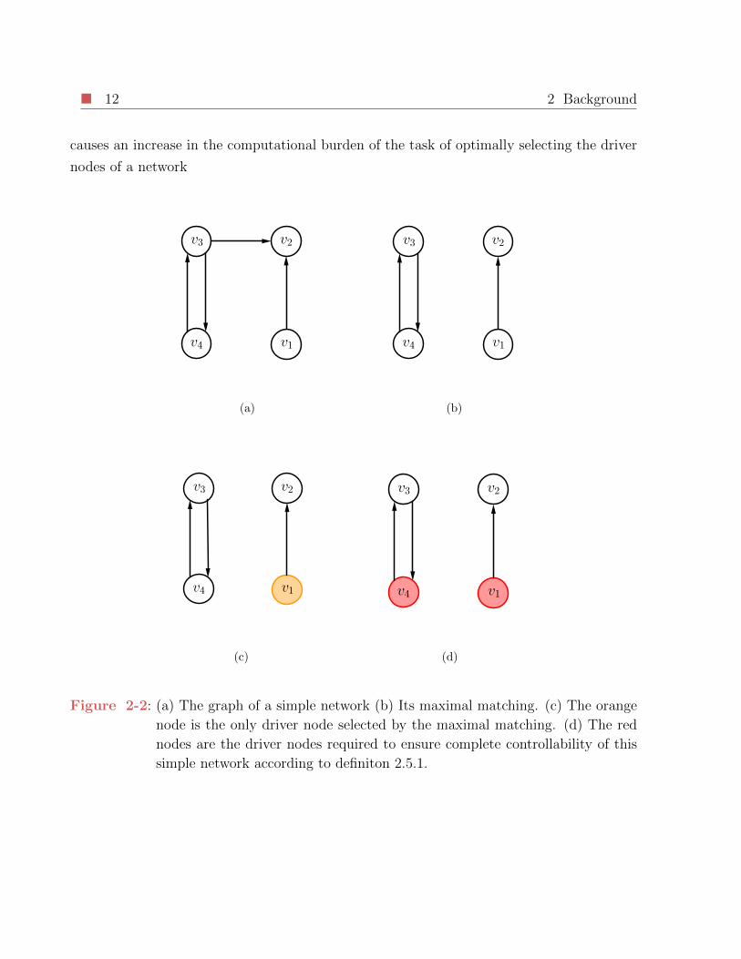
12 2 Background
causes an increase in the computational burden of the task of optimally selecting the driver
nodes of a network
(a) (b)
(c) (d)
Figure 2-2: (a) The graph of a simple network (b) Its maximal matching. (c) The orange
node is the only driver node selected by the maximal matching. (d) The red
nodes are the driver nodes required to ensure complete controllability of this
simple network according to definiton 2.5.1.
CHAPTER 3
Partial Controllability of Complex
Networks
In Chapter 2, we have introduced controllability as a property that must be conferred to
a network. Nevertheless, the perspective taken in this thesis is that ensuring a network be
completely controllable is, more often than not, a chimera for two distinct reasons. Firstly,
the scale of complex networks is often such that too many driver nodes would be required to
fulfill such an ambitious requirement. To put things in perspective, consider that the complex
networks paradigm has been proposed to model biological systems such as cellular networks
[28]. Who could imagine to arbitrarily impose the state of all the cells of an organism?
This same example brings us to our second point, complex systems have not been built
to be controlled. The features of biological systems are mostly result of the evolution of
species, the structure and functions of social networks vary with the number and characters
of the people who enter these networks, and finally the structure of real world technological
systems such as power grids grows and changes depending on the needs of the end users to
be served. Hardly any of these complex systems are designed explicitly taking into account
that the need can arise of controlling their behavior. Hence, it is reasonable to imagine that
the access to nodes that can be crucial to guarantee complete controllability of the network
might be precluded.
Motivated by these considerations, in this thesis we cope with the problem of developing
driver node selection algorithms that allow maximizing the number of controllable nodes of
a network while taking into account the economic and physical constraints that inevitably
arise in applications. Before giving a formal statement of the main problem addressed in
this thesis, let us define formally what we mean when we refer to the set of structurally
controllable nodes of a network. As anticipated in Section 2.4.1, while the dimension of
14 3 Partial Controllability of Complex Networks
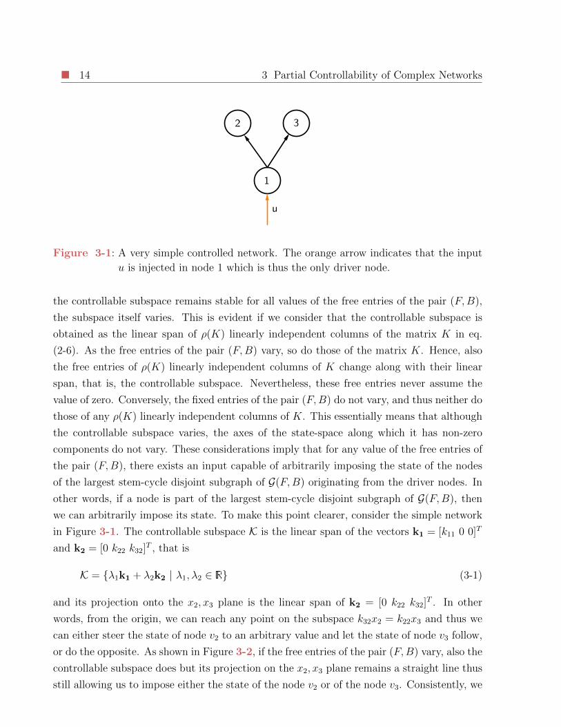
Figure 3-1: A very simple controlled network. The orange arrow indicates that the input
u is injected in node 1 which is thus the only driver node.
the controllable subspace remains stable for all values of the free entries of the pair (F,B),
the subspace itself varies. This is evident if we consider that the controllable subspace is
obtained as the linear span of ρ(K) linearly independent columns of the matrix K in eq.
(2-6). As the free entries of the pair (F,B) vary, so do those of the matrix K. Hence, also
the free entries of ρ(K) linearly independent columns of K change along with their linear
span, that is, the controllable subspace. Nevertheless, these free entries never assume the
value of zero. Conversely, the fixed entries of the pair (F,B) do not vary, and thus neither do
those of any ρ(K) linearly independent columns of K. This essentially means that although
the controllable subspace varies, the axes of the state-space along which it has non-zero
components do not vary. These considerations imply that for any value of the free entries of
the pair (F,B), there exists an input capable of arbitrarily imposing the state of the nodes
of the largest stem-cycle disjoint subgraph of G(F,B) originating from the driver nodes. In
other words, if a node is part of the largest stem-cycle disjoint subgraph of G(F,B), then
we can arbitrarily impose its state. To make this point clearer, consider the simple network
in Figure 3-1. The controllable subspace K is the linear span of the vectors k1 = [k11 0 0]T
and k2 = [0 k22 k32]T , that is
K = λ1k1 + λ2k2 | λ1, λ2 ∈ R (3-1)
and its projection onto the x2, x3 plane is the linear span of k2 = [0 k22 k32]T . In other
words, from the origin, we can reach any point on the subspace k32x2 = k22x3 and thus we
can either steer the state of node v2 to an arbitrary value and let the state of node v3 follow,
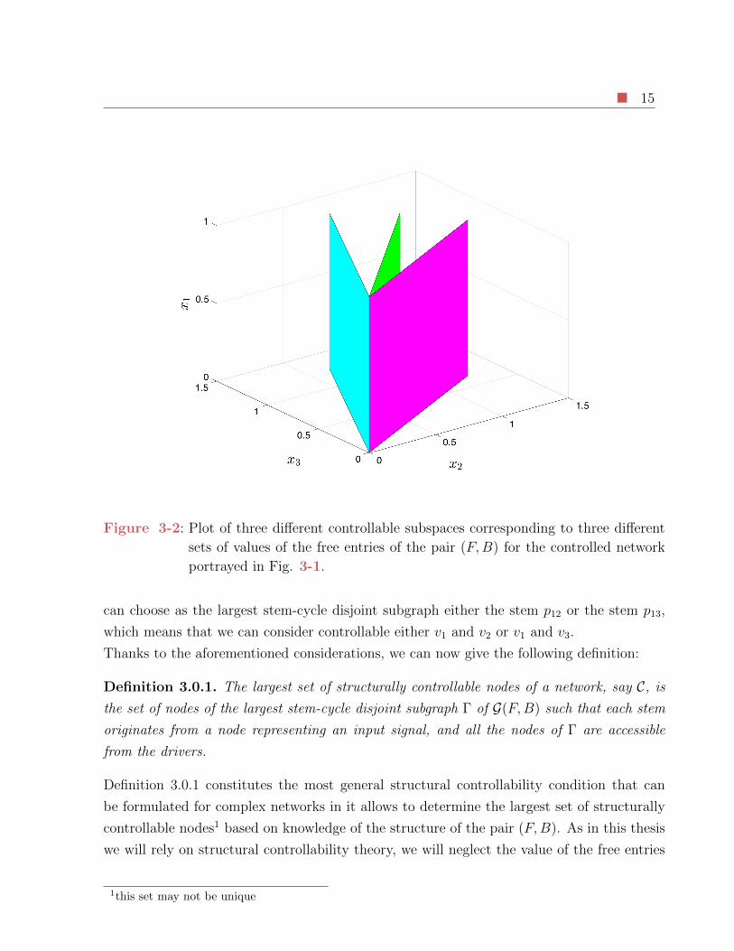
or do the opposite. As shown in Figure 3-2, if the free entries of the pair (F,B) vary, also the
controllable subspace does but its projection on the x2, x3 plane remains a straight line thus
still allowing us to impose either the state of the node v2 or of the node v3. Consistently, we
15
Figure 3-2: Plot of three different controllable subspaces corresponding to three different
sets of values of the free entries of the pair (F,B) for the controlled network
portrayed in Fig. 3-1.
can choose as the largest stem-cycle disjoint subgraph either the stem p12 or the stem p13,
which means that we can consider controllable either v1 and v2 or v1 and v3.
Thanks to the aforementioned considerations, we can now give the following definition:
Definition 3.0.1. The largest set of structurally controllable nodes of a network, say C, is
the set of nodes of the largest stem-cycle disjoint subgraph Γ of G(F,B) such that each stem
originates from a node representing an input signal, and all the nodes of Γ are accessible
from the drivers.
Definition 3.0.1 constitutes the most general structural controllability condition that can
be formulated for complex networks in it allows to determine the largest set of structurally
controllable nodes1 based on knowledge of the structure of the pair (F,B). As in this thesis
we will rely on structural controllability theory, we will neglect the value of the free entries
1this set may not be unique

16 3 Partial Controllability of Complex Networks
of the matrix F in equation (2-4). Hence, for simplicity, we will know on represent the
dynamics of a linear dynamical network as
x = Ax, (3-2)
where each unit entry of the adjacency matrix A indicates the presence of a free entry in the
matrix F in eq. (2-4), the exact value of which is unknown. We will resort to eq. (2-4) only
if necessary and in this case we will explicitly refer to it.
In Chapter 2 we underlined that according to Liu et al. [37], in the complex network
paradigm, controllability may be posed as the problem of selecting the minimal set of driver
nodes that ensures the generic dimension of the controllable subspace be N . Following the
same line of argument, but departing from the point of view that achieving complete struc-
tural controllability of a complex network is more often than not a chimera, in this thesis,
we pose partial controllability of complex networks as the problem of selecting a set of nodes
of fixed cardinality that maximizes the number of structurally controllable nodes. Moreover,
to allow taking into account the constraints that inevitably arise in applications, we consider
the case in which restrictions apply on the selection of the driver nodes. Specifically, we con-
sider the case in which controllability is sought of a well-specified set of target nodes. This
is the case, for instance, when attempting to design curative interventions for cancer, as one
is typically interested in acting only on cells lying in carcinogenic and pre-carcinogenic state
[68, 42]. Moreover, we take into account the case in which the selection of the driver nodes is
restricted to a well-defined subset of the nodes of the network. A typical scenario of applica-
tion of this condition is the design of curative interventions, when only some easily accessible
proteins are designated as targets for drugs [29, 15, 44]. Finally, we allow considering the
case in which the need arises of exerting these control actions without perturbing some nodes
which are assigned to particularly important or vital functions. Some of these constraints
have been recently considered in [13], where a heuristic strategy is proposed for selecting the
driver nodes ensuring controllability of a set of target nodes. However, as stated in [13], a
geometrical mapping of this problems is still lacking. In this thesis, we provide a toolbox
of algorithms that allow tackling driver node selection problems for partial controllability of
complex networks.
3.1 Problem Formulation
To give a formal statement of the main problem tackled in this thesis, we must first introduce
the following notation.

3.1 Problem Formulation 17
• We denote by Ω ⊂ V the set of admissible nodes of a network, that is, the set of nodes
that can be selected as drivers;
• We denote by ΩD ⊂ Ω the set of nodes selected as drivers;
• We denote by Φ ⊂ V the set of target nodes, that is, the nodes of a network that must
be made structurally controllable;
• We denote by Ψ ⊂ V the set of untouchable nodes, that is, the nodes of a network that
must not be perturbed by the control action;
• We denote by Ξi ⊂ V the set of nodes in the upstream of node vi;
• Given a set Θ, we denote by |Θ| its cardinality, that is, the number of its elements.
We can now formally state the main problem addressed in this thesis:
maxΩD
|C| (3-3)
s.t.
|ΩD| = M (3-4)
ΩD ⊂ Ω (3-5)
Φ ⊂ C (3-6)
( ∪i|vi∈Ψ
Ξi) ∩ ΩD = ∅. (3-7)
Equations (3-3) and (3-4) translate the general problem of finding the set of driver nodes ΩD
of cardinality M that maximizes the number of controllable nodes. Moreover eqs. (3-5)-(3-7)
formalize respectively the constraints that the driver nodes must be selected from the set of
admissible nodes Ω, that the target nodes must be made controllable, and that the set of
untouchable nodes Ψ must not be perturbed by the control action. Figure 3-3 illustrates a
possible scenario of application of the stated problem.
The problem in eqs. (3-3)-(3-7) is stated in terms of sets of nodes as the toolbox of algo-
rithms we provide to find its solution is mainly based on fulfilling graphical conditions. To
conclude the transition presented in this chapter from the classical algebraic interpretation of
controllability of linear systems to its graphical mapping leveraged in this thesis, we provide
an algebraic interpretation of eqs. (3-3)-(3-4). Namely, we structure the input matrix B
so to maximize the dimension of the controllable subspace with the constraint that B must
have M columns each being a vector with only one free entry. If the entry bij of the matrix
B is free, then node vi has been selected as a driver node.
18 3 Partial Controllability of Complex Networks
Figure 3-3: A possible scenario of application of the problem in equations (3-3)-(3-7). The
green circles represent the nodes of the set Ω, the red cicles the nodes of Ψ,
and the blue circles the nodes of Φ.
3.2 Problem Solution
To solve the problem in eqs. (3-3)-(3-7), the first step is that of deriving a graphical condition
that ensures the selection of the set of driver nodes ΩD is optimal. Indeed, the starting
point must be Definition 3.0.1 which states that the generic dimension of the controlallable
subspace is equal to the dimension of the largest stem-cycle disjoint subgraph Γ of G(A,B)
such that all stems originate from the nodes representing the input signals, and all cycles are
in the downstream of the nodes representing the input signals. Unfortunately, such condition
is based on knowledge of the matrix B and thus on the set of driver nodes ΩD which in our
problem is obviously unknown. Hence, the graphical condition to be defined must determine
the set ΩD rather than depending on it.
Lemma 3.2.1. The set of driver nodes ΩD of fixed cardinality M that maximizes the num-
ber of structurally controllable nodes of a network |C| is given by the sources of the largest
subgraph Γc of G(A) such that
• Γc is stem-cycle disjoint;
3.2 Problem Solution 19
• Γc has M stems;
• each cycle of Γc is accessible, in G(A) from at least one source of the M stems.
We choose as metric of the dimension of the subgraph Γc the number of its nodes.
In the condition defined in Lemma 3.2.1, we elect to change the metric of the dimension of
a subgraph from the number of its edges to the number of its nodes. In definition 3.0.1,
the chosen metric is the number of edges as the graph G(A,B) encompasses an additional
set of nodes representing the input signals. Hence, measuring the dimension of the largest
stem-cycle disjoint subgraph as the number of its nodes would lead to an overestimation of
the dimension of the controllable subspace. On the other hand, as in stems and cycles each
node has only one inbounding edge except for the sources of the stems which have none,
measuring the dimension of the stem-cycle disjoint subgraph of G(A,B) as the number of
its edges allows to ingore the nodes representing the input signals thus correctly evaluating
the dimension of the controllable subspace. Here, ΩD is to be determined and thus we must
reason only on the graph of the network G(A). Hence, measuring the dimension of Γc as the
number of its edges would lead to ignore the sources of the stems while chosing as a metric
the number of its nodes allows correctly evaluating |C|.On the ground of Lemma 3.2.1, we can now give the algorithm developed to solve the prob-
lem in equations (3-3)-(3-7). Our algorithm is built in two phases. Firstly, starting from the
graph G(A), we build an augmented graph G ′ that may be partitioned into disjoint cycles.
Then, we formulate an ILP that performs an optimal cycle partition of G ′ by eliminating
some of its edges. Removing, from the optimal cycle partition, the nodes and edges that are
not part of the graph G we find the stem-cycle disjoint subgraphs Γc fulfills the condition
expressed in Lemma 3.2.1 plus a set of isolated vertexes: the uncontrollable nodes. With
this intuitive explanation in mind, we can now go through the steps of our algorithm.
Algorithm 1
Steps 1-7, construction of the graph G ′:
1. G ′(V ′,P ′) = G(V ,P).
2. Find the set Ω′ = Ω− ∪i|vi∈ΨΞi ⊆ Ω of admissible nodes that do not have a vertex
of Ψ in their downstream.
3. Add, to G ′, a set of M new nodes, say Θ, representing the M input signals to be
injected in the network.

20 3 Partial Controllability of Complex Networks
4. Remove, from G ′ all the nodes of Ψ and their upstream, along with all the associated
edges.
5. Add |Θ| × |Ω′| new edges exiting each node of Θ and entering each node of Ω′.
6. Add |Θ| × (|V ′| − |Θ|) new edges exiting each node of G ′ that is also a node of G and
entering each node of Θ.
7. Add a self loop one for each node of G ′ that is not a node of Θ nor of Φ.
Steps 8-11, finding the optimal cycle partition of G ′:
8 Associate a binary decision variable yij to each edge p′ij of G ′.
9 Associate a unit weight wij to each decision variable yij that is either:
– associated with an edge p′ij of G ′ that is also an edge of G;
– associated with an edge p′ij of G ′ that exits a node of Θ;
10 Associate zero weight w′ij to all the other decision variables yij:
11 Solve the following Integer Linear Program:
maxy
∑i
∑j
w′ijyij (3-8)
subject to
yij ∈ 0, 1 ∀i, j|p′ij ∈ P ′ (3-9)∑j
yij = 1 ∀i = 1, ..., N +M (3-10)∑i
yij = 1 ∀j = 1, ..., N +M (3-11)∑l∈Ξi
∑j∈Θ
ylj ≥∑j
w′ijyij ∀i = 1, ..., N +M (3-12)
The proposed algorithm first builds an augmented graph G ′ in which the M input signals
to be injected in the network are represented as additional nodes belonging to a set Θ. The
edges exiting the nodes of Θ point only to the nodes of Ω′, so to restrict the selection of the
drivers to the admissible nodes that do not have any untouchable node in their downstream.
Instead, the added edges that point to the nodes of Θ (step 5) allow reducing the M stems
originating from the additional nodes to cycles. Finally, in order to make sure there exists a
cycle partition of G ′, self loops are added to each node of G ′ that is not a target node.

3.2 Problem Solution 21
Now, the problem in eqs. (3-3)-(3-7) can be translated into a problem on the graph G ′. We
must select, among all the cycle partitions of G ′, the one that encompasses the maximum
number of edges p′ij that are also edges of G satisfying the following constraint: the nodes
in cycles encompassing edges p′ij that are also edges of G must be accessible, in G, from the
nodes selected as drivers.
This problem translates into the Integer Linear Program (ILP) in eqs. (3-8)-(3-12). Specifi-
cally, a binary decision variable yij is associated with each edge p′ij of the graph G ′; if yij = 1,
then the corresponding edge p′ij will be part of the cycle partition. The product w′ijyij will
return a unit cost either when the selected edge of G ′ is also an edge of G or if the edge exits
a node of Θ. As, in the cycle partition, the edges exiting the nodes of Θ enter the nodes that
are selected as drivers, these are constrained to be M as prescribed by eq. (3-10). Hence,
eq. (3-8) translates the goal of maximizing the number of edges of G ′ that are also edges
of G. Moreover, as the nodes of the cycle partition with an inbounding edge of unit weight
compose the set C, and as all edges with unit weight only enter nodes of G ′ that are also
nodes of G, eq. (3-8) represents the maximal achievable cardinality of the set of controllable
nodes thanks to Lemma 3.2.1. Every other selected edge will not contribute to the objective
function and is to be viewed as a slack variable as it is only needed to form a cycle.
The role of the constraints of the ILP is that of ensuring the solution fulfills the requirements
of the problem in eqs. (3-3)-(3-7). Namely, eqs. (3-10) and (3-11) guarantee that the optimal
solution be a cycle partition of G ′ by forcing each one of its vertices to have exactly one
entering and one outgoing edge, while eq. (3-12) forces all the nodes of C to be accessible
from at least one of the driver nodes. This is done by ensuring that if a node has an entering
edge with unit weight then there is at least a node in its upstream that has an edge with
unit weight entering it that exits from a node of Θ. Note that the constraints on the target,
admissible, and untouchable nodes in eqs. (3-5)-(3-7) are fulfilled through the construction
of the graph G ′. Namely, thanks to steps 2 and 5, all the nodes that are in the upstream
of the untouchable nodes do not have an inbounding edge that exits the nodes of Θ, thus
ensuring that the nodes of the set Ψ are not perturbed by control signals. Morover, thanks
to step 7, the target nodes do not have inbounding edges with zero wight and thus must be
included in the set C. Finally, thanks to step 5, only the admissible nodes can be selected
as drivers.
An example of application of our method when M = 1 is shown in figure 3-4; the orange
node in figure 3-4b) represents the input signal, while the orange and blue edges are those
added to enable the formation of a cycle partition. The nodes with inbounding black or
orange edges are those encompassed in C.
22 3 Partial Controllability of Complex Networks
Figure 3-4: An example of application of our method
The developed algorithm us to deal, as particular cases, with the following two relevant
problems.
a. Finding the node with maximum centrality When (i) the set Ω coincides with the
entire set of vertices of G and (ii) the sets Φ and Ψ are empty, specifying our algorithm for
M = 1 allows us to determine the node with maximum control centrality [38].
b. Finding the largest set of controllable nodes given the set of driver nodes
(Hosoe’s theorem) When (i) the set ΩD is given and (ii) the sets Φ and Ψ are empty,
the proposed algorithm allows us to determine the set of controllable nodes, given the set of
driver nodes. Note that in this scenario, our algorithm reduces to Poljak’s [49] method as
the set ΩD is given and no driver node has to be selected.
Feasibility of the proposed method We rely on the implicit assumption that our method
is applied to a well formulated problem, i.e., a problem that admits a solution. However,
this would not be the case, for instance, if an untouchable node were in the downstream of a
target node, as for the latter to be controllable, the former must be influenced. We remark
that the feasibility issues are not related to our method but to the problem itself. Hence, if
our method does not output a solution, then a solution to the problem does not exist in the
structural controllability framework.
As anticipated, the viewpoint taken in this thesis is that gaining full control of complex
networks is, more often than not, a chimera leading us to shift our perspective towards con-
trolling just a fraction of the network nodes. Equations (3-3)-(3-7) translate this conceptual
idea in the problem of finding the set of driver nodes ΩD of fixed cardinality that maximizes
the cardinality |C| of the set of structurally controllable nodes of a network. In what follows,
3.2 Problem Solution 23
we propose a formulation that translates the same conceptual idea of controlling only a frac-
tion of the network nodes into a different optimization problem, namely that of finding the
set of driver nodes of minimum cardinality that allows achieving structural controllability
of a well defined set of target nodes Φ while fulfilling the constraints on admissible and
untouchable nodes:
minΩD⊂Ω
|ΩD| (3-13)
subject to
Φ ⊂ C
∪i∈Ψ (Ξi) ∩ ΩD = ∅.
Coping with this problem requires only minor tweaks to the algorithm described above. As
the number of driver nodes is now to be determined and is bounded by the cardinality of
Ω′, in step 3 we will have that |Θ| = |Ω′| as |Ω′| new nodes representing input signals must
be added to the graph G ′. Moreover, as it is possible that less than |Ω′| driver nodes are
required to ensure structural controllability of the set Φ, in step 7, a self loop must be added
to each of the nodes of Θ. Furthermore, the objective function of the ILP (Eq. (3-8)) must
now read
minyij |vj∈Θ
∑j|vj∈Θ
∑i
w′ijyij. (3-14)
Thus, in this case, a cycle partition is sought that minimizes the number of driver nodes
necessary to fulfill the requirement on the target and untouchable nodes. The vertices
representing input signals that are not injected in the network form cycles of their own
thanks to the additional self loops. Again, our algorithm assumes that the problem is well
formulated, i.e., that it admits a solution in the structural controllability framework. Again
this general formulation allows us to cope, as particular cases, with two prominent problems.
a. Finding the MDS of a network If (i) the sets Ω and Φ coincide with the entire set of
vertices and (ii) Ψ is empty, solving the problem in equation (3-13) corresponds to finding the
set of driver nodes of minimum cardinality that ensure complete controllability of a network
[37].
b. Target Controllability When (i) Ω coincides with the entire set of vertices, (ii) Ψ is
empty, and (iii) Φ is a well defined subset of nodes, solving solving the problem in equation
(3-13) allows to find an optimal solution to the problem for which a heuristic strategy is
proposed in [13].

24 3 Partial Controllability of Complex Networks
3.3 Computational Considerations
Research on complex networks has always been closely tied to computational issues for two
distinct reasons. First of all, complex networks are large scale systems and for this simple
reason any tool or method easily used for low-dimensional dynamical systems might turn
out requiring too much computational power when applied to complex networks. For in-
stance, as highlighted by Steven Strogatz in his distinguished review [59], only of late the
availability of powerful computers has made it feasible to probe the structure of complex net-
works. Second of all, most choice problems that translate into graph optimization problems
are solved by performing a second translation into ILPs. Notable examples are the shortest
path problem, scheduling problems, or the well-known traveling salesman problem. Driver
node selection problems for complex networks make no exception to this general rule as,
leveraging the structural controllability theory, they can be translated into graph optimiza-
tion problems. As shown in the previous section, the latter can again be translated into ILPs
thanks to the general algorithm proposed in this thesis. Unfortunately, ILPs are, in general,
Non-deterministic Polynomial time hard (NP-hard). Without entering into the details of
computational complexity theory (which is beyond the scope of this thesis), this means that
there is no guarantee these problems can be solved in polynomial time, although there is no
proof of the opposite as well.
The fact that ILPs are, in general, NP-hard does not mean that any problem that admits a
translation into an ILP is actually NP-hard. For instance, the shortest path problem is best
formulated as an ILP but can be solved performing a relaxation to a Linear Program (LP),
that is, ignoring the integer constraint on the decision variables, which makes the problem
solvable in (weakly) polynomial time. Moreover, several problems that naturally translate
into ILPs admit ad-hoc algorithms capable of finding the optimal solution. In fact, nobody
would ever solve a shortest path problem by solving the associated LP as several much faster
algorithms have been developed to find the optimal solution.
From these considerations, the question of if driver node selection problems can be solved
in polynomial time naturally arises. Let us start providing an answer by discussing the case
of finding the minimal set of driver nodes (MDS) necessary to ensure complete structural
controllability of a complex network, that is, the problem dealt with in ref [37]. If relying
on definition 2.5.1, finding the MDS of a network ultimately reduces to solving an ILP
the objective function of which is defined in equation (3-14) subject to the constraints in
equations (3-9)-(3-12). The question becomes: is it possible to relax the ILP to an LP
which, in general, can be solved in (weakly) polynomial time and still obtain an integer
3.3 Computational Considerations 25
solution? The algebraic condition that ensures the solution of an LP be integer is that the
matrix defined by its constraints is totally unimodular and that the constant terms are all
integers. In this case, the polytope defined by the constraints has vertices with only integer
coordinates. As it is well known that the solution of a Linear Program lies on a vertex of the
polytope defined by its constraints, it follows that if the matrix defined by the constraints of
an ILP is totally unimodular, and if the constant terms are all integers, then the solution of
the LP relaxation of an ILP is also the solution of the ILP. By inspecting equations (3-10)-
(3-12) we can immediately note that the constant terms of our constraints are all integers.
Moreover, the matrix defined by the equality constraints in eqs. (3-10) and (3-11) is totally
unimodular as it verifies the sufficient condition given in Lemma 2.2.1. Namely, we note that
all the free entries of the matrix defined in equations (3-10) and (3-11) take the value of 1,
and thus, performing the decomposition in two blocks I1 and I2 proposed in Lemma 2.2.1,
we have that one of the two, say I1, is empty while the other, say I2, encompasses all the
matrix. Moreover, we note that each each column of the matrix contains only two non-zero
entries. This as each decision variable yij represents an edge p′ij of the graph G ′, and thus
it is encompassed only once in the constraint in equation (3-10) which ensures that in the
optimal cycle node vj has only one edge exiting it and once in the constraint in equation
(3-11) which ensures that in the optimal cycle partition node vi has only one edge exiting
it. As the constraints in equations (3-10) and (3-11) force the solution of the ILP be a cycle
partition of the graph G ′, this means that finding a cycle partition of a graph is a problem
that can be solved in polynomial time. Going back to our problem, unfortunately equation
(3-17) spoils the total unimodularity of the constraint matrix of our ILP. Thus, adopting
definition 2.5.1 we obtain that finding the MDS of a network is a problem that cannot be
solved in polynomial time. As underlined in section 3.2, the constraint in eq. (3-17) ensures
each node of C be accessible from a driver node in the graph G. Here, we add that considering
this constraint is what differentiates definition 2.5.1 from that given by Liu et al. in ref. [37].
This as if a cycle is not accessible from at least a node where a control signal is injected, then
a control signal must be injected in an arbitrary node of the inaccessible cycle to guarantee
controllability of all of its nodes. Nevertheless, as this control signal can be the same as
that injected in any other node of the network, the number of distinct control signals to be
injected in the network in order to ensure the latter be completely structurally controllable
does not change. Hence, adopting the definition of a driver node given in [37] ensures the
problem of finding the MDS of a network is solvable in polynomial time. This comes at
the price of not being able to determine the complete structure of the matrix B. Moreover,
the perspective taken in this thesis is that limitations are often imposed on the number of
26 3 Partial Controllability of Complex Networks
nodes in which a signal is injected, rather than on the number of distinct signals deployed
for the control action. Finally, from an energetic standpoint, injecting the same signal into
two different nodes may be inefficient as the same control action is used to achieve a larger
number of objectives. To better understand this point consider the problem of steering the
linear dynamical system
x = Ax +Bu (3-15)
where u(t) = [u1(t) u2(t)]T , from an initial state x(0) to a desired final state x(t1). In order
to minimize the energy required to achieve the control goal, u(t) is chosen as the solution of
the following optimization problem:
minu(t)
J :=
∫ t1
0
u(t)Tu(t)dt, (3-16)
As imposing u1(t) = u2(t) represents a constraint for the optimization problem in (3-16),
bounding two signals to be identical can only yield an increase in the optimal J .
To provide a general answer to the question of if the driver nodes selection strategy pro-
posed in this thesis is NP-hard we point out that solving the problem in equations (3-3)-(3-7)
requires solving the ILP in equations (3-8)-(3-12). Again equation (3-12) ensures the con-
straint matrix is not totally unimodular and thus also finding the set of driver nodes of fixed
cardinality so to maximize the number of controllable nodes of a network is NP-hard.
Given the NP-hard nature of the ILP in equations (3-8)-(3-12) the following question nat-
urally arises: does it prove unsolvable for large networks? Absolutely not. As testified by
the numerical results reported in the next chapter, we have solved millions of instances of
the ILP in eqs. (3-8)-(3-12) for networks of up to 104 nodes and we have never been forced
to resort to heuristic strategies. Instead, we focused on finding the strongest possible for-
mulation of our problem. To obtain this strengthened formulation, in the construction of G ′
we only add one additional node representing all the input signals (step 3 of our algorithm).
This node, denoted as N + 1, now plays the role of all the nodes of Θ and is connected to
all of the other N nodes of G ′ with both inbounding and outgoing edges. Node N + 1 has
the ability to close all of the M cycles that include a driver node. Coherently, the equality
3.3 Computational Considerations 27
constraints in Eqs. (3-10) and (3-11) are changed to∑j
yij = 1 ∀i = 1, ..., N (3-17)∑i
yij = 1 ∀j = 1, ..., N (3-18)∑j
yN+1,j = M (3-19)∑i
yi,N+1 = M. (3-20)
The advantage of this new formulation is that it considerably reduces both the number of
variables and the number of constraints. Namely, the number of variables that this new
formulation allows to remove is |V ′| × (M − 1) + |Ω′| × (M − 1) as instead of adding M new
nodes representing the input signals which must then be connected with outgoing edges to
all the nodes of Ω′ and with inbounding edges with all the nodes of the graph G ′, we only
add one. Moreover, the number of constraints is reduced by 2× (M − 1) as again only one
node is added to represent the M input signals and thus only two additional constraints
must be considered to force the edges exiting and entering this node be M instead of 2M
additional constraints ensuring each node of Θ has one entering and one exiting edge. Note
that the proposed strengthened formulation is sill characterized by the total unimodularity
of the matrix defined by the constraints (3-17)-(3-20). This as equation (3-17) is the same as
equation (3-10) except for it only holds for j = 1, ..., N instead of j = 1, ..., N+M . Moreover,
the same reasoning applies to the relationship between equations (3-18) and (3-18). Finally,
as equation (3-19) is the same as N + 1-th constraint defined by equation (3-17) only with
a constant term that is still integer but equals to M , and the same reasoning applies to the
relationship between equation (3-20) and the N+1-th constraint defined by equation (3-18),
the condition in Lemma 2.2.1 is still verified.
Although all numerical results reported in this thesis have been obtained using the strength-
ened fomrulation in eqs. (3-17)-(3-20) but only relying on standard ILP solvers such as
those implemented in Matlab and Gurobi, for completeness, we have developed an ad-hoc
algorithm for the solution of our ILP based on the property that the equality constraint
matrix is totally unimodular. As we will show in what follows, this structural property can
be exploited to strongly reduce the computational complexity of the ILP. The idea behind
our strategy is that of complementing the general Branch and Cut techniques used to solve
ILPs with ad hoc bounding and cutting procedures able to exploit the special structure of
our problem.
Bounding: estimation of an upper bound for |C|. An approximation of |C| from above can

28 3 Partial Controllability of Complex Networks
be obtained from a relaxed version of our problem.
Relaxation A: a first relaxation can be obtained, as usual, by removing the integrity con-
straints on the decision variables yij thus transforming the ILP into an LP. Note that as the
equality constraint matrix is totally unimodular often this relaxation will yield an integer
solution allowing the ILP to stop at the root LP solution. This as several vertexes of the
polytope defined by the entire set of constraints in equations (3-12) and (3-17)-(3-20) will
be also vertices of the totally unimodular matrix defined by the constraints in (3-17)-(3-20),
which we know are integer.
Relaxation B: a second strategy is that of relaxing constraint (3-12). In this case the prob-
lem becomes that of finding the cycle partition of G ′ that maximizes our objective function.
As the equality constraint matrix is totally unimodular, also this problem reduces to a LP.
Obviously, in bounding from above the objective function of problem (3-8) - (3-12) the min-
imum between the two estimates can be selected.
Bounding: estimation of a lower bound for |C|. An approximation from below of the number
of controllable nodes can be obtained from Relaxation B. Indeed, the solution of the relaxed
problem offers a cycle covering of the graph G ′ for which not necessarily each cycle is acces-
sible from the drivers. By subtracting the number of nodes located in inaccessible cycles to
the objective function we get the approximation required.
Ad hoc Cutting procedures The branching phase in ILP solution methods is always com-
plemented with a cutting procedure. Cuts are additional constraints added to the ILP that
allow strengthening the formulation without eliminating feasible solutions. In our case, if the
upper bound resulting from Relaxation A is tighter, then standard cuts (Gomory, Strong,
etc.) and binary branching strategies are to be applied (although always taking into ac-
count the availability of a lower bound). On the other hand, if the upper bound obtained
by relaxing the constraints in (3-12) is tighter, then two ad hoc cutting strategies can be
deployed which exploit the structure of our problem. Both consist in applying recursively
some constraints.
Strategy 1: The first ad hoc cutting strategy consists of the following steps:
1. Relax the constraints in Eq. (3-12) and solve the LP relaxation of the resulting ILP.
The solution will be integer as the equality constraint matrix is totally unimodular.
This yields a set of driver nodes Ω1D and a set of controllable nodes C1;
2. If each node of C1 is accessible from at least one node of Ω1D then the optimal solution
is found;
3. Otherwise, |C1| is an upper bound for the optimal value |C∗|;

3.3 Computational Considerations 29
4. Remove the inaccessible nodes from C1 to obtain a lower bound for |C∗| along with the
largest set of controllable nodes from the set of drivers Ω1D;
5. Apply the inequality constraint∑l∈Ω1
D
yl,N+1 ≤M − 1 (3-21)
to exclude the set Ω1D from the possible sets of drivers and solve the LP relaxation of
the new ILP.;
6. If the solution is integer but unfeasible as some cycles are inaccessible, two new bounds
can be computed as in steps 3 and 4. Take the tightest among the available bounds and
repeat steps 5 and 6 until either an integer feasible solution or a non-integer feasible
solution is found;
7. If an integer feasible solution is found, then the optimal solution is the best one between
such solution and the current lower bound;
8. If on the other hand a non-integer solution is found, then this is the tightest possible
upper bound. Now, the standard cuts and branching strategies must be applied (tak-
ing into account the availability of upper and lower bounds to enhance the pruning
procedure).
Strategy 2: The first four steps of the second ad hoc cutting strategy coincide with the first
four steps of Strategy 1. These must be complemented by the following steps;
5. Amongst the inequality constraints in (3-12) apply only those violated by the solution
obtained at step 1;
6. If the solution is integer but unfeasible, as some cycles are inaccessible, two new bounds
can be computed as in steps 3 and 4. Take the tightest among the available bounds and
repeat steps 5 and 6 until either an integer feasible solution or a non-integer feasible
solution is found;
7. If the solution is integer and feasible, then it is optimal;
8. If the solution is non-integer and feasible, then this is the tightest possible upper bound.
Now, the standard cuts and branching strategies must be applied (taking into account
the availability of upper and lower bounds to enhance the pruning procedure).

30 3 Partial Controllability of Complex Networks
The idea behind both cutting strategies is that the sequence of upper and lower bounds
obtained by exploiting the total unimodularity of the equality constraint matrix can drive
the search toward the true solution. While these strategies have been designed to complement
standard branch and cut algorithms in order to find the optimal solution, if the search is
stopped before the solution is found (because it exceeds the maximum time, for instance) an
interval of uncertainty on the number of controllable nodes is obtained along with (at least)
a feasible solution. Hence, the two defined strategies can also be viewed as simple heuristics.
In the next chapter, we will discuss some more sophisticated heuristics which have been
developed in order to cope with driver node selection problems in huge complex networks
(networks with over 105 nodes).
CHAPTER 4
Structural Permeability of Complex
Networks to Control Signals
In Chapter 2 we have defined controllability of a linear dynamical system as a structural
property of the pair (F,B) in equation (2-5). Moreover, we have underlined that in the com-
plex network paradigm we have to view controllability as a property that must be conferred
to a network as, more often than not, the driver nodes are not given a priori but must be
selected. Still, as shown by Liu et al. in ref [37] the network structure may facilitate, or
hinder, our ability to make a network structurally controllable. Namely, the authors link
the propensity of the network structure to be made completely controllable to its degree
distribution and, relying on the cavity method [45, 67], they derive a set of self-consistent
equations able to predict the number of driver nodes required to achieve complete controlla-
bility of a network based on the degree distribution of its topology. By applying the cavity
method to several real and model network topologies, they find that sparse heterogeneous
networks are harder to be made completely controllable than dense homogeneous networks.
The authors also provide numerical evidence confirming their analytic predictions.
Spurred by these results, several researchers have studied the relation between the network
structure and its propensity to be made completely structurally controllable. For instance,
Ruths and Ruths [55] have studied the network motifs that affect controllability, while Liu
et al. [38] the relation between the network degree distribution and its maximum control
centrality, that is, the dimension of the largest set of controllable nodes achievable by lever-
aging only one driver node. Then, driven by the same idea of linking our ability to control a
network to its structure, researchers have crossed the boundary of structural controllability.
For instance, Nepusz and Vicsek [46] have explored the option of introducing a dynamical
process on the network edges and found that the controllability properties of this process
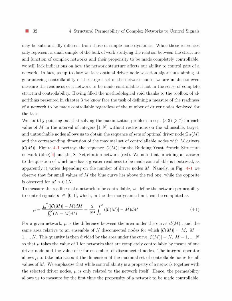
32 4 Structural Permeability of Complex Networks to Control Signals
may be substantially different from those of simple node dynamics. While these references
only represent a small sample of the bulk of work studying the relation between the structure
and function of complex networks and their propensity to be made completely controllable,
we still lack indications on how the network structure affects our ability to control part of a
network. In fact, as up to date we lack optimal driver node selection algorithms aiming at
guaranteeing controllability of the largest set of the network nodes, we are unable to even
measure the readiness of a network to be made controllable if not in the sense of complete
structural controllability. Having filled the methodological void thanks to the toolbox of al-
gorithms presented in chapter 3 we know face the task of defining a measure of the readiness
of a network to be made controllable regardless of the number of driver nodes deployed for
the task.
We start by pointing out that solving the maximization problem in eqs. (3-3)-(3-7) for each
value of M in the interval of integers [1, N ] without restrictions on the admissible, target,
and untouchable nodes allows us to obtain the sequence of sets of optimal driver node ΩD(M)
and the corresponding dimension of the maximal set of controlallable nodes with M drivers
|C(M)|. Figure 4-1 portrays the sequence |C(M)| for the Budding Yeast Protein Structure
network (blue)[4] and the SciNet citation network (red). We note that providing an answer
to the question of which one has a greater readiness to be made controllable is nontrivial, as
apparently it varies depending on the number of driver nodes M . Namely, in Fig. 4-1 we
observe that for small values of M the blue curve lies above the red one, while the opposite
is observed for M > 0.1N .
To measure the readiness of a network to be controllable, we define the network permeability
to control signals µ ∈ [0, 1], which, in the thermodynamic limit, can be computed as
µ =
∫ N0
(|C(M)| −M)dM∫ N0
(N −M)dM=
2
N2
∫ N
0
(|C(M)| −M)dM (4-1)
For a given network, µ is the difference between the area under the curve |C(M)|, and the
same area relative to an ensemble of N disconnected nodes for which |C(M)| = M, M =
1, ..., N . This quantity is then divided by the area under the curve |C(M)| = N, M = 1, ..., N
so that µ takes the value of 1 for networks that are completely controllable by means of one
driver node and the value of 0 for ensembles of disconnected nodes. The integral operator
allows µ to take into account the dimension of the maximal set of controllable nodes for all
values of M . We emphasize that while controllability is a property of a network together with
the selected driver nodes, µ is only related to the network itself. Hence, the permeability
allows us to measure for the first time the propensity of a network to be made controllable,
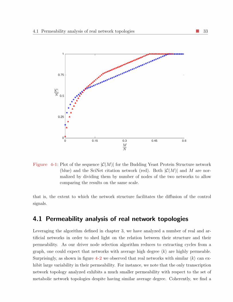
4.1 Permeability analysis of real network topologies 33
Figure 4-1: Plot of the sequence |C(M)| for the Budding Yeast Protein Structure network
(blue) and the SciNet citation network (red). Both |C(M)| and M are nor-
malized by dividing them by number of nodes of the two networks to allow
comparing the results on the same scale.
that is, the extent to which the network structure facilitates the diffusion of the control
signals.
4.1 Permeability analysis of real network topologies
Leveraging the algorithm defined in chapter 3, we have analyzed a number of real and ar-
tificial networks in order to shed light on the relation between their structure and their
permeability. As our driver node selection algorithm reduces to extracting cycles from a
graph, one could expect that networks with average high degree 〈k〉 are highly permeable.
Surprisingly, as shown in figure 4-2 we observed that real networks with similar 〈k〉 can ex-
hibit large variability in their permeability. For instance, we note that the only transcription
network topology analyzed exhibits a much smaller permeability with respect to the set of
metabolic network topologies despite having similar average degree. Coherently, we find a
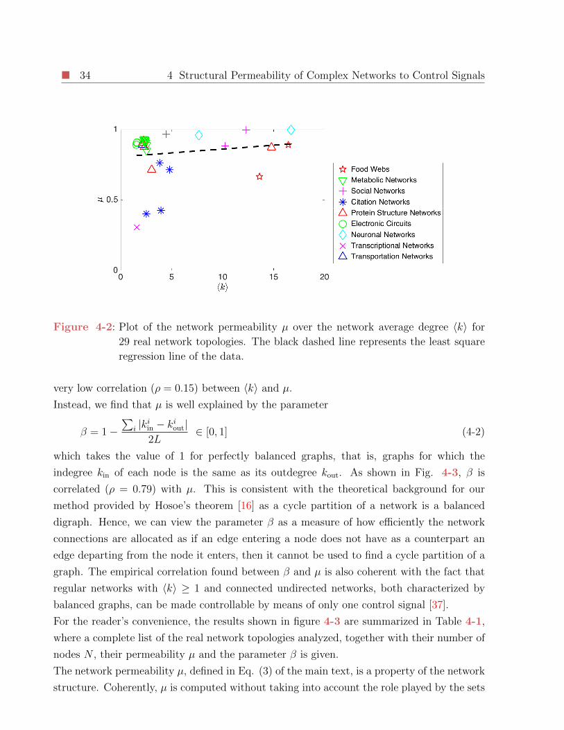
34 4 Structural Permeability of Complex Networks to Control Signals
Figure 4-2: Plot of the network permeability µ over the network average degree 〈k〉 for
29 real network topologies. The black dashed line represents the least square
regression line of the data.
very low correlation (ρ = 0.15) between 〈k〉 and µ.
Instead, we find that µ is well explained by the parameter
β = 1−∑
i |kiin − kiout|2L
∈ [0, 1] (4-2)
which takes the value of 1 for perfectly balanced graphs, that is, graphs for which the
indegree kin of each node is the same as its outdegree kout. As shown in Fig. 4-3, β is
correlated (ρ = 0.79) with µ. This is consistent with the theoretical background for our
method provided by Hosoe’s theorem [16] as a cycle partition of a network is a balanced
digraph. Hence, we can view the parameter β as a measure of how efficiently the network
connections are allocated as if an edge entering a node does not have as a counterpart an
edge departing from the node it enters, then it cannot be used to find a cycle partition of a
graph. The empirical correlation found between β and µ is also coherent with the fact that
regular networks with 〈k〉 ≥ 1 and connected undirected networks, both characterized by
balanced graphs, can be made controllable by means of only one control signal [37].
For the reader’s convenience, the results shown in figure 4-3 are summarized in Table 4-1,
where a complete list of the real network topologies analyzed, together with their number of
nodes N , their permeability µ and the parameter β is given.
The network permeability µ, defined in Eq. (3) of the main text, is a property of the network
structure. Coherently, µ is computed without taking into account the role played by the sets
4.1 Permeability analysis of real network topologies 35
Figure 4-3: Plot of the network permeability µ over the parameter β for 30 real network
topologies. The black dashed line represents the least square regression line of
the data.
Ω, Φ, and Ψ, as reasonably the constraints on admissible, target and untouchable nodes are
related to specific scenarios of application of our method. The permeability µ thus takes the
limit value of 0 for an ensemble of disconnected nodes, as the diffusion of signals is prevented
by the absence of connectivity and each node can be made controllable only if it is a driver.
This corresponds to the worst case scenario in terms of permeability. Nevertheless, when
the sets Ω and Ψ are considered, some nodes of the network become inaccessible directly
and indirectly. Namely, in order to ensure the control signals do not reach the nodes of the
set Ψ, all the untouchable nodes and all the nodes in their upstream cannot be selected as
drivers. Hence, they can neither be made controllable directly nor indirectly. The same line
of argument extends to the case of the admissible nodes. Namely, if a nodes is not part
of the set Ω, nor it is accessible from a node of the latter set, then it can neither be made
controllable directly nor indirectly. As for the presence of target nodes, while these do not
affect our ability to control any specific node, their presence might make the optimization
problem in (3-3)-(3-7) unfeasible. This corresponds to the situation in which there does not
exists a set of driver nodes ΩD ⊂ Ω of dimension M that ensures structural controllability
of the set of target nodes Φ.
Summing up, in the presence of untouchable and target nodes, and when the set of admissible
nodes does not correspond to the entire set of network nodes, the (approximate) computation
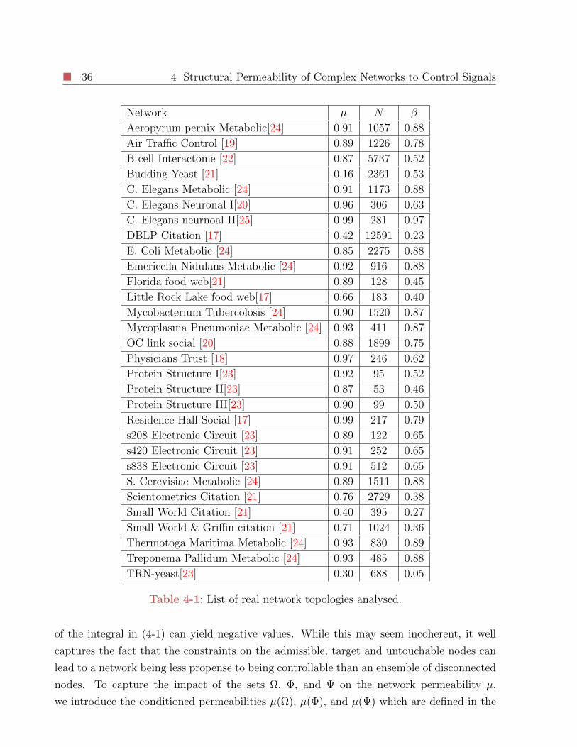
36 4 Structural Permeability of Complex Networks to Control Signals
Network µ N β
Aeropyrum pernix Metabolic[24] 0.91 1057 0.88
Air Traffic Control [19] 0.89 1226 0.78
B cell Interactome [22] 0.87 5737 0.52
Budding Yeast [21] 0.16 2361 0.53
C. Elegans Metabolic [24] 0.91 1173 0.88
C. Elegans Neuronal I[20] 0.96 306 0.63
C. Elegans neurnoal II[25] 0.99 281 0.97
DBLP Citation [17] 0.42 12591 0.23
E. Coli Metabolic [24] 0.85 2275 0.88
Emericella Nidulans Metabolic [24] 0.92 916 0.88
Florida food web[21] 0.89 128 0.45
Little Rock Lake food web[17] 0.66 183 0.40
Mycobacterium Tubercolosis [24] 0.90 1520 0.87
Mycoplasma Pneumoniae Metabolic [24] 0.93 411 0.87
OC link social [20] 0.88 1899 0.75
Physicians Trust [18] 0.97 246 0.62
Protein Structure I[23] 0.92 95 0.52
Protein Structure II[23] 0.87 53 0.46
Protein Structure III[23] 0.90 99 0.50
Residence Hall Social [17] 0.99 217 0.79
s208 Electronic Circuit [23] 0.89 122 0.65
s420 Electronic Circuit [23] 0.91 252 0.65
s838 Electronic Circuit [23] 0.91 512 0.65
S. Cerevisiae Metabolic [24] 0.89 1511 0.88
Scientometrics Citation [21] 0.76 2729 0.38
Small World Citation [21] 0.40 395 0.27
Small World & Griffin citation [21] 0.71 1024 0.36
Thermotoga Maritima Metabolic [24] 0.93 830 0.89
Treponema Pallidum Metabolic [24] 0.93 485 0.88
TRN-yeast[23] 0.30 688 0.05
Table 4-1: List of real network topologies analysed.
of the integral in (4-1) can yield negative values. While this may seem incoherent, it well
captures the fact that the constraints on the admissible, target and untouchable nodes can
lead to a network being less propense to being controllable than an ensemble of disconnected
nodes. To capture the impact of the sets Ω, Φ, and Ψ on the network permeability µ,
we introduce the conditioned permeabilities µ(Ω), µ(Φ), and µ(Ψ) which are defined in the
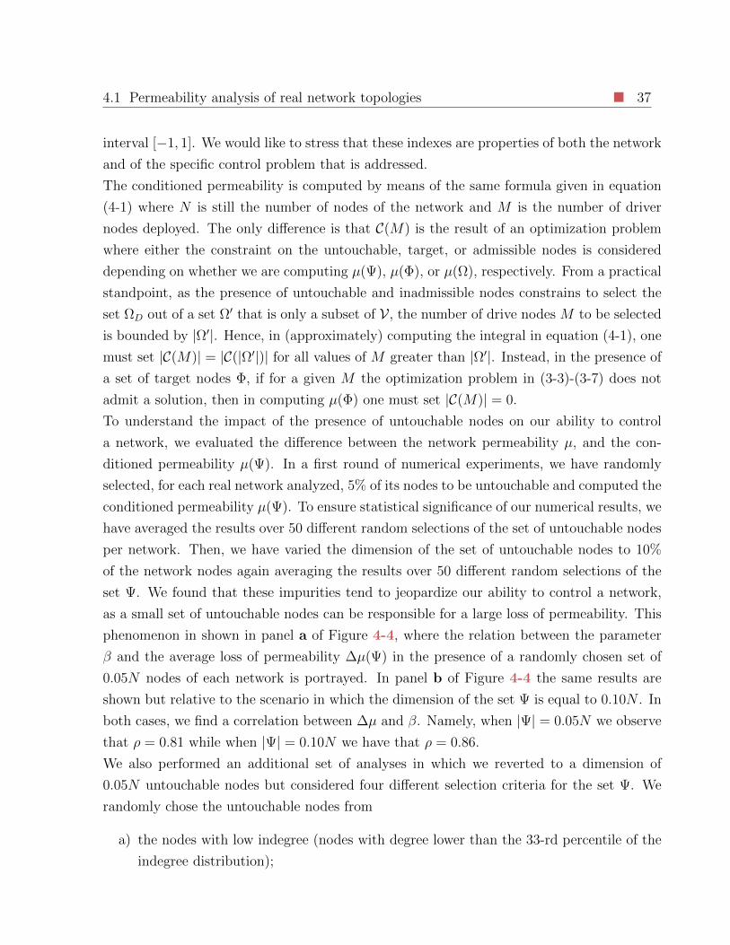
4.1 Permeability analysis of real network topologies 37
interval [−1, 1]. We would like to stress that these indexes are properties of both the network
and of the specific control problem that is addressed.
The conditioned permeability is computed by means of the same formula given in equation
(4-1) where N is still the number of nodes of the network and M is the number of driver
nodes deployed. The only difference is that C(M) is the result of an optimization problem
where either the constraint on the untouchable, target, or admissible nodes is considered
depending on whether we are computing µ(Ψ), µ(Φ), or µ(Ω), respectively. From a practical
standpoint, as the presence of untouchable and inadmissible nodes constrains to select the
set ΩD out of a set Ω′ that is only a subset of V , the number of drive nodes M to be selected
is bounded by |Ω′|. Hence, in (approximately) computing the integral in equation (4-1), one
must set |C(M)| = |C(|Ω′|)| for all values of M greater than |Ω′|. Instead, in the presence of
a set of target nodes Φ, if for a given M the optimization problem in (3-3)-(3-7) does not
admit a solution, then in computing µ(Φ) one must set |C(M)| = 0.
To understand the impact of the presence of untouchable nodes on our ability to control
a network, we evaluated the difference between the network permeability µ, and the con-
ditioned permeability µ(Ψ). In a first round of numerical experiments, we have randomly
selected, for each real network analyzed, 5% of its nodes to be untouchable and computed the
conditioned permeability µ(Ψ). To ensure statistical significance of our numerical results, we
have averaged the results over 50 different random selections of the set of untouchable nodes
per network. Then, we have varied the dimension of the set of untouchable nodes to 10%
of the network nodes again averaging the results over 50 different random selections of the
set Ψ. We found that these impurities tend to jeopardize our ability to control a network,
as a small set of untouchable nodes can be responsible for a large loss of permeability. This
phenomenon in shown in panel a of Figure 4-4, where the relation between the parameter
β and the average loss of permeability ∆µ(Ψ) in the presence of a randomly chosen set of
0.05N nodes of each network is portrayed. In panel b of Figure 4-4 the same results are
shown but relative to the scenario in which the dimension of the set Ψ is equal to 0.10N . In
both cases, we find a correlation between ∆µ and β. Namely, when |Ψ| = 0.05N we observe
that ρ = 0.81 while when |Ψ| = 0.10N we have that ρ = 0.86.
We also performed an additional set of analyses in which we reverted to a dimension of
0.05N untouchable nodes but considered four different selection criteria for the set Ψ. We
randomly chose the untouchable nodes from
a) the nodes with low indegree (nodes with degree lower than the 33-rd percentile of the
indegree distribution);
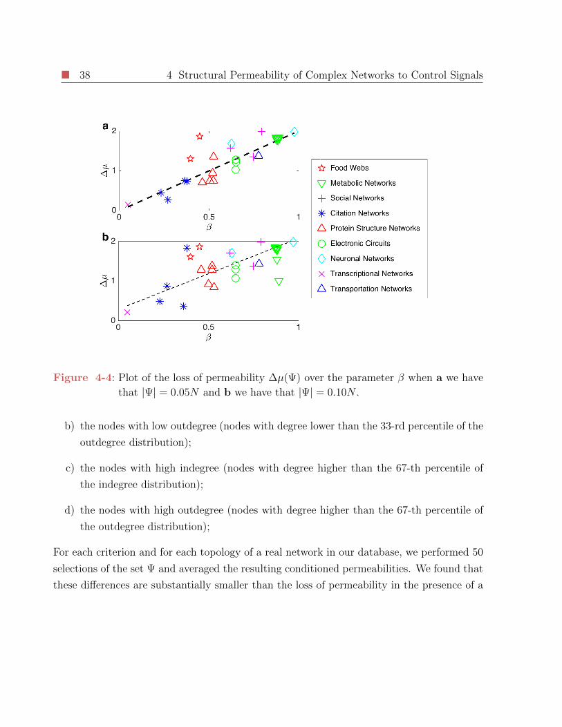
38 4 Structural Permeability of Complex Networks to Control Signals
Figure 4-4: Plot of the loss of permeability ∆µ(Ψ) over the parameter β when a we have
that |Ψ| = 0.05N and b we have that |Ψ| = 0.10N .
b) the nodes with low outdegree (nodes with degree lower than the 33-rd percentile of the
outdegree distribution);
c) the nodes with high indegree (nodes with degree higher than the 67-th percentile of
the indegree distribution);
d) the nodes with high outdegree (nodes with degree higher than the 67-th percentile of
the outdegree distribution);
For each criterion and for each topology of a real network in our database, we performed 50
selections of the set Ψ and averaged the resulting conditioned permeabilities. We found that
these differences are substantially smaller than the loss of permeability in the presence of a
4.1 Permeability analysis of real network topologies 39
completely random extraction of the set Ψ. Specifically, we found that⟨(∆µ(Ψa)−∆µ(Ψr))2
(∆µ(Ψr))2
⟩= 0.12,⟨
(∆µ(Ψb)−∆µ(Ψr))2
(∆µ(Ψr))2
⟩= 0.02,⟨
(∆µ(Ψc)−∆µ(Ψr))2
(∆µ(Ψr))2
⟩= 0.01,⟨
(∆µ(Ψd)−∆µ(Ψr))2
(∆µ(Ψr))2
⟩= 0.04,
where:
• µ is the permeability of the network;
• ∆µ(Ψi) = µ − µ(Ψi) is the permeability conditioned to the presence of untouchable
nodes selected according to the i-th criterion;
• ∆µ(Ψr) = µ − µ(Ψr) is the permeability conditioned to the presence of completely
randomly selected untouchable nodes (the criterion used in the main text of the paper);
• 〈·〉 indicates that the quantities are averaged over the networks in our databases and
over 50 different extractions of the sets Ψi.
Moreover, Figure 4-5 shows that the correlation between the loss of permeability ∆µ(Ψi)
and β, when applied to all of the networks in our dataset, is confirmed, irrespective of the
specific selection criterion considered. In fact, ∆µ(Ψa), ∆µ(Ψb), ∆µ(Ψc), and ∆µ(Ψd) have
a correlation with β of 0.86, 0.86, 0.84, and 0.85, respectively.
The previous numerical analyses were aimed at uncovering the relation between the network
structure and its readiness to be made controllable regardless of the number of drivers de-
ployed for the task. The shift of perspective proposed in this thesis, from complete to partial
controllability, and the associated toolbox of algorithms presented in chapter 3 allow us to
also uncover the structural features of the network nodes that determine their controllability
properties. By solving the optimization problem in equations (3-3)-(3-7) without restrictions
on the set of admissible, target, and untouchable nodes we can obtain the full composition
of the set of controllable nodes C(M) and of its complement C(M). In performing our nu-
merical studies, we kept track of the structural properties of the nodes of these sets in order
to uncover the structural properties of the nodes that can be made easily controllable. We
found that the nodes of both C(M) and C(M) are characterized by signatures. Namely, the

40 4 Structural Permeability of Complex Networks to Control Signals
Figure 4-5: Plot of the loss of permeability ∆µ(Ψ) over the parameter β. The title of each
panel corresponds to the criterion with which the set of untouchable nodes
responsible of the loss of permeability was selected.
nodes of C(M) exhibit higher degree than those of its complement C(M) as shown in Fig.
4-6(a).
After having structurally characterized the nodes that tend to fall in the set C from those
that require a large number of driver nodes to be included in the optimal set of controllable
nodes, we turn our attention to the structural properties of the set of optimal driver nodes
ΩD. In ref [37], Liu et al. found that when applying the maximal matching algorithm, input
signals were usually injected in nodes with low degree. This finding is labeled as surprising
as the authors expected the hubs to play a key role in network control. Being able to select
optimal sets of driver nodes ΩD of any dimension in the interval [0, N ], allows us take a
step forward in the analysis of the structural properties of the optimal driver nodes. By
observing Figure 4-1, we note that for small values of M the marginal increments in the
dimension of the set of controllable nodes |C(M)| − |C(M − 1)| are larger than those that
are experienced when M is large. This spurs us to study the structural properties of the
nodes that are selected as drivers when M is small, as these often allow controlling a large
fraction of the network nodes. We find that when M is small, the nodes of ΩD(M) typically
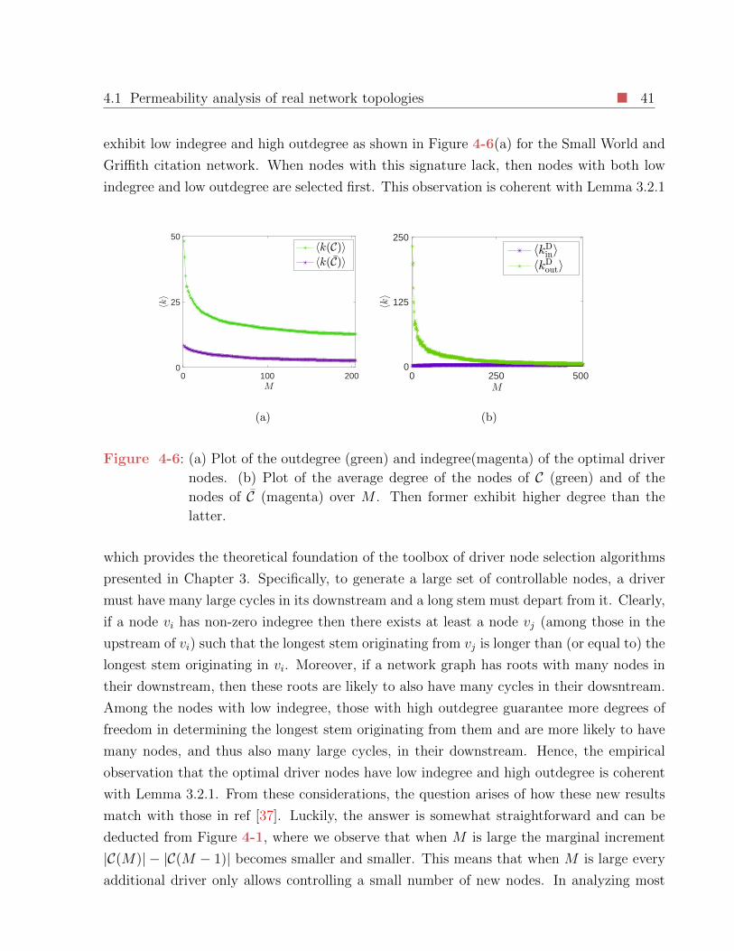
4.1 Permeability analysis of real network topologies 41
exhibit low indegree and high outdegree as shown in Figure 4-6(a) for the Small World and
Griffith citation network. When nodes with this signature lack, then nodes with both low
indegree and low outdegree are selected first. This observation is coherent with Lemma 3.2.1
0 100 200M
0
25
50
hki
hk(C)ihk( 7C)i
(a)
0 250 500M
0
125
250
hki
hkDini
hkDouti
(b)
Figure 4-6: (a) Plot of the outdegree (green) and indegree(magenta) of the optimal driver
nodes. (b) Plot of the average degree of the nodes of C (green) and of the
nodes of C (magenta) over M . Then former exhibit higher degree than the
latter.
which provides the theoretical foundation of the toolbox of driver node selection algorithms
presented in Chapter 3. Specifically, to generate a large set of controllable nodes, a driver
must have many large cycles in its downstream and a long stem must depart from it. Clearly,
if a node vi has non-zero indegree then there exists at least a node vj (among those in the
upstream of vi) such that the longest stem originating from vj is longer than (or equal to) the
longest stem originating in vi. Moreover, if a network graph has roots with many nodes in
their downstream, then these roots are likely to also have many cycles in their dowsntream.
Among the nodes with low indegree, those with high outdegree guarantee more degrees of
freedom in determining the longest stem originating from them and are more likely to have
many nodes, and thus also many large cycles, in their downstream. Hence, the empirical
observation that the optimal driver nodes have low indegree and high outdegree is coherent
with Lemma 3.2.1. From these considerations, the question arises of how these new results
match with those in ref [37]. Luckily, the answer is somewhat straightforward and can be
deducted from Figure 4-1, where we observe that when M is large the marginal increment
|C(M)| − |C(M − 1)| becomes smaller and smaller. This means that when M is large every
additional driver only allows controlling a small number of new nodes. In analyzing most
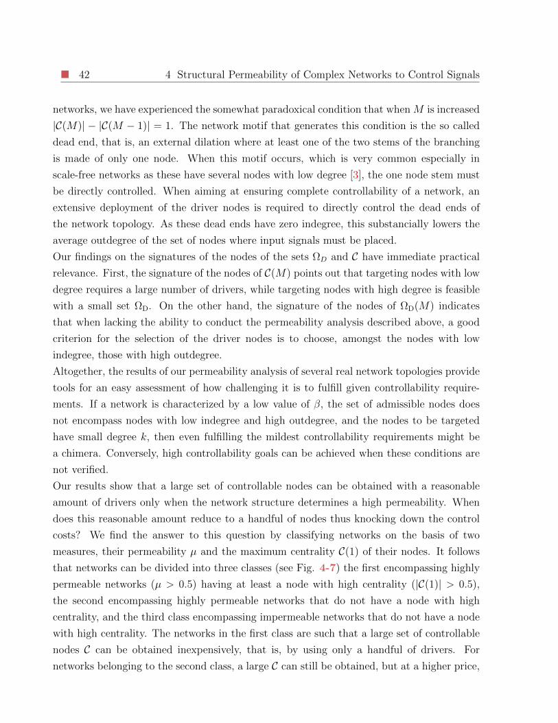
42 4 Structural Permeability of Complex Networks to Control Signals
networks, we have experienced the somewhat paradoxical condition that when M is increased
|C(M)| − |C(M − 1)| = 1. The network motif that generates this condition is the so called
dead end, that is, an external dilation where at least one of the two stems of the branching
is made of only one node. When this motif occurs, which is very common especially in
scale-free networks as these have several nodes with low degree [3], the one node stem must
be directly controlled. When aiming at ensuring complete controllability of a network, an
extensive deployment of the driver nodes is required to directly control the dead ends of
the network topology. As these dead ends have zero indegree, this substancially lowers the
average outdegree of the set of nodes where input signals must be placed.
Our findings on the signatures of the nodes of the sets ΩD and C have immediate practical
relevance. First, the signature of the nodes of C(M) points out that targeting nodes with low
degree requires a large number of drivers, while targeting nodes with high degree is feasible
with a small set ΩD. On the other hand, the signature of the nodes of ΩD(M) indicates
that when lacking the ability to conduct the permeability analysis described above, a good
criterion for the selection of the driver nodes is to choose, amongst the nodes with low
indegree, those with high outdegree.
Altogether, the results of our permeability analysis of several real network topologies provide
tools for an easy assessment of how challenging it is to fulfill given controllability require-
ments. If a network is characterized by a low value of β, the set of admissible nodes does
not encompass nodes with low indegree and high outdegree, and the nodes to be targeted
have small degree k, then even fulfilling the mildest controllability requirements might be
a chimera. Conversely, high controllability goals can be achieved when these conditions are
not verified.
Our results show that a large set of controllable nodes can be obtained with a reasonable
amount of drivers only when the network structure determines a high permeability. When
does this reasonable amount reduce to a handful of nodes thus knocking down the control
costs? We find the answer to this question by classifying networks on the basis of two
measures, their permeability µ and the maximum centrality C(1) of their nodes. It follows
that networks can be divided into three classes (see Fig. 4-7) the first encompassing highly
permeable networks (µ > 0.5) having at least a node with high centrality (|C(1)| > 0.5),
the second encompassing highly permeable networks that do not have a node with high
centrality, and the third class encompassing impermeable networks that do not have a node
with high centrality. The networks in the first class are such that a large set of controllable
nodes C can be obtained inexpensively, that is, by using only a handful of drivers. For
networks belonging to the second class, a large C can still be obtained, but at a higher price,
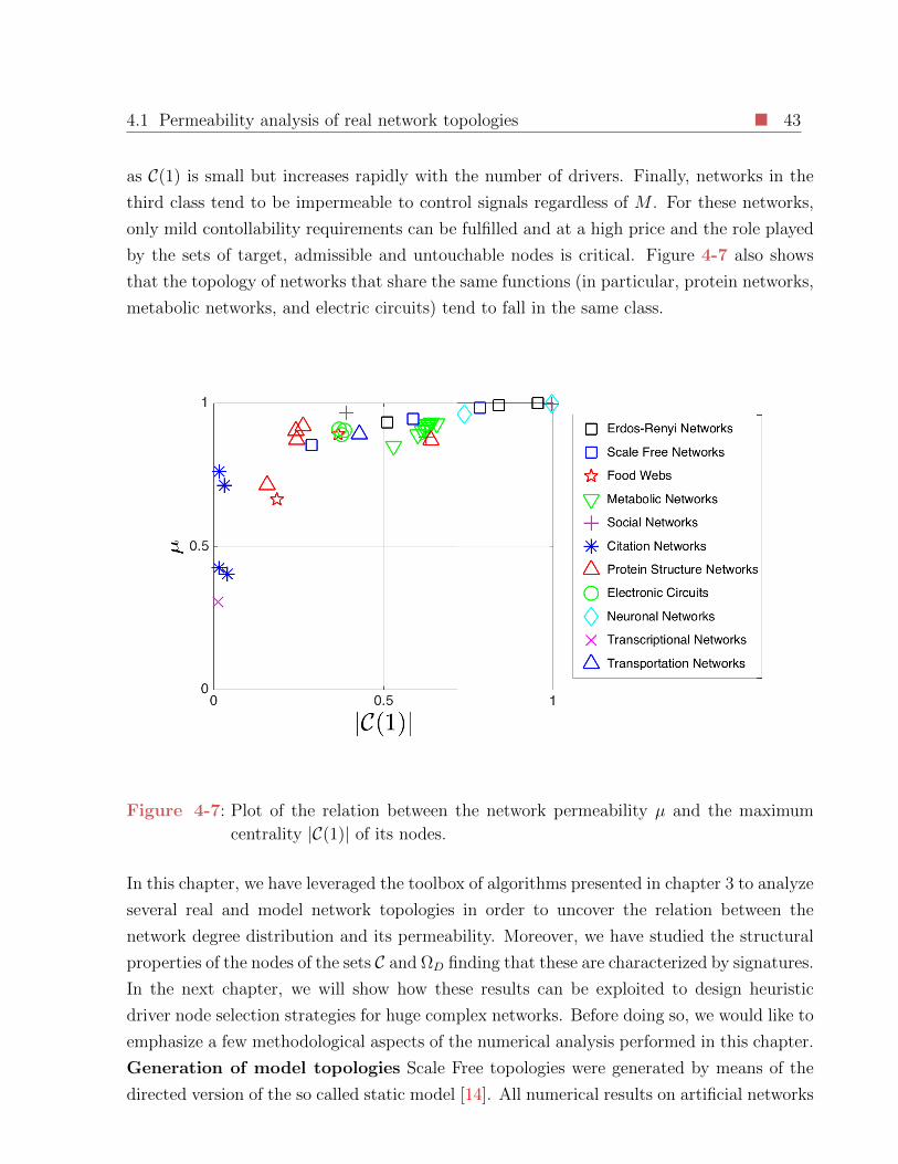
4.1 Permeability analysis of real network topologies 43
as C(1) is small but increases rapidly with the number of drivers. Finally, networks in the
third class tend to be impermeable to control signals regardless of M . For these networks,
only mild contollability requirements can be fulfilled and at a high price and the role played
by the sets of target, admissible and untouchable nodes is critical. Figure 4-7 also shows
that the topology of networks that share the same functions (in particular, protein networks,
metabolic networks, and electric circuits) tend to fall in the same class.
Figure 4-7: Plot of the relation between the network permeability µ and the maximum
centrality |C(1)| of its nodes.
In this chapter, we have leveraged the toolbox of algorithms presented in chapter 3 to analyze
several real and model network topologies in order to uncover the relation between the
network degree distribution and its permeability. Moreover, we have studied the structural
properties of the nodes of the sets C and ΩD finding that these are characterized by signatures.
In the next chapter, we will show how these results can be exploited to design heuristic
driver node selection strategies for huge complex networks. Before doing so, we would like to
emphasize a few methodological aspects of the numerical analysis performed in this chapter.
Generation of model topologies Scale Free topologies were generated by means of the
directed version of the so called static model [14]. All numerical results on artificial networks

44 4 Structural Permeability of Complex Networks to Control Signals
are averaged over 100 topologies of 1000 nodes each.
Integer Linear Programming solver The numerical analysis was conducted on the Mat-
lab platform by using the integer linear programming solver intlinprog or the Gurobi add-on.
We emphasize that the method we propose can be implemented also on other available com-
mercial software. All the presented results are exact as we have never been forced to settle
for an approximation of the optimal solution due to limitations on the execution time of our
algorithm.
CHAPTER 5
Heuristic Driver Node Selection
Strategies
In Chapter 4 we have performed an analysis of several real and model networks in order to
uncover the structural properties that influence the network permeability µ. In doing so, we
also kept track of the characteristics of the nodes of the optimal set of drivers ΩD and of the
resulting set of controllable nodes C(M). In this chapter, we take advantage of the findings
described in Chapter 4 to design heuristic driver node selection strategies that exploit the
network structure in order to maximize the number of controllable nodes. We will thus
refer to the optimization problem in equations (3-3)-(3-7) without taking into account the
constraints on admissible, target, and untouchable nodes.
The main goal of the proposed heuristic strategies is twofold. First of all, although we never
ran into an unsolvable instance of the ILP in equations (3-8)-(3-12), that is, the dreaded
worst-case scenario which could arise due to its NP-hard nature, we aim at providing the
readership with a sub-optimal strategy should this case arise. Secondly, as is the case
for all graph-optimization problems, the scale of our ILP grows with the dimension of the
network. As we will see, the strategies proposed in this chapter allow reducing the scale of
the optimization problem to be solved.
We start discussing our heuristic strategies by recalling that the ILP in equations (3-8)-(3-12)
is made NP-hard by the constraints in equation (3-12). These constraints only ensure that all
the elements of the set of controllable nodes be accessible from the driver nodes. On the other
hand, finding an optimal cycle partition of a graph, that is, the task performed in equations
(3-8)-(3-11), can be performed in polynomial time. Hence, in our heuristic strategies we aim
at decoupling these two tasks. To do so, we start by recalling that according to Lemma
3.2.1, for a node to be controllable, it must either be part of a stem originating from a driver

46 5 Heuristic Driver Node Selection Strategies
node or part of a cycle accessible from a driver node. As all of the nodes of a stem are
accessible from its source by definition, the accessibility constraints in equation (3-12) only
come into play if the graph of a network contains cycles. Otherwise they are redundant and
do not alter the polytope defined by the constraints in (3-10),(3-11). As we have shown that
the matrix defined by the latter constraints is totally unimodular we can give the following
Lemma.
Lemma 5.0.1. If the graph G of a network is a DAG, then the ILP in equations (3-8)-(3-12)
that must be solved in order to select a set of driver nodes of fixed cardinality M to maximize
the number of controllable nodes is not NP-hard.
The relevance of Lemma 5.0.1 goes beyond its statement in it allows tailoring an heuristic
strategy to networks that encompass very few, small cycles.
Heuristic Strategy 1: If the maximum number of nodes of a network that can be included in
disjoint cycles by only leveraging the network graph G is small, then a good heuristic strategy
for selecting the driver nodes so to maximize the number of controllable nodes can be obtained
by applying the algorithm for the exact solution of our problem while neglecting the constraints
in equation (3-12) and then removing, from the resulting stem-cycle disjoint subgraph, the
cycles that are not accessible from the drivers. We will denote the set of controllable nodes
obtained leveraging on Heuristic Strategy 1 by C1(M)
The rationale behind this heuristic strategy is very simple. If the network graph is such
that very few of its nodes can be included in disjoint cycles, than we may as well relax
the accessibility constraints and solve a problem that is not NP-hard. This will lead to a
slight overestimation of |C| as some inaccessible cycles might be included in the stem-cycle
disjoint subgraph resulting from the solution of the relaxed ILP. Nevertheless, by eliminating
the inaccessible cycles we should obtain a set of controllable nodes C1(M) the dimension of
which should be close to the actual optimal solution C∗(M).
As we have anticipated, Heuristic Strategy 1 is to be used if only a small number of nodes
can be included in disjoint cycles by only leveraging the edges of the graph of the network.
While we will leave to later the explanation of the criteria based on which one can determine
whether the number of nodes that can be included in disjoint cycles is neglectable, a key
aspect that must be immediately discussed is how to determine this number. One trivial
way, is to apply Algorithm 1 assuming M = 0 and neglecting the accessibility constraints
in equation (3-12) when solving the ILP (which thus becomes of complexity P). While this
strategy allows exactly computing the number of nodes that can be included in disjoint
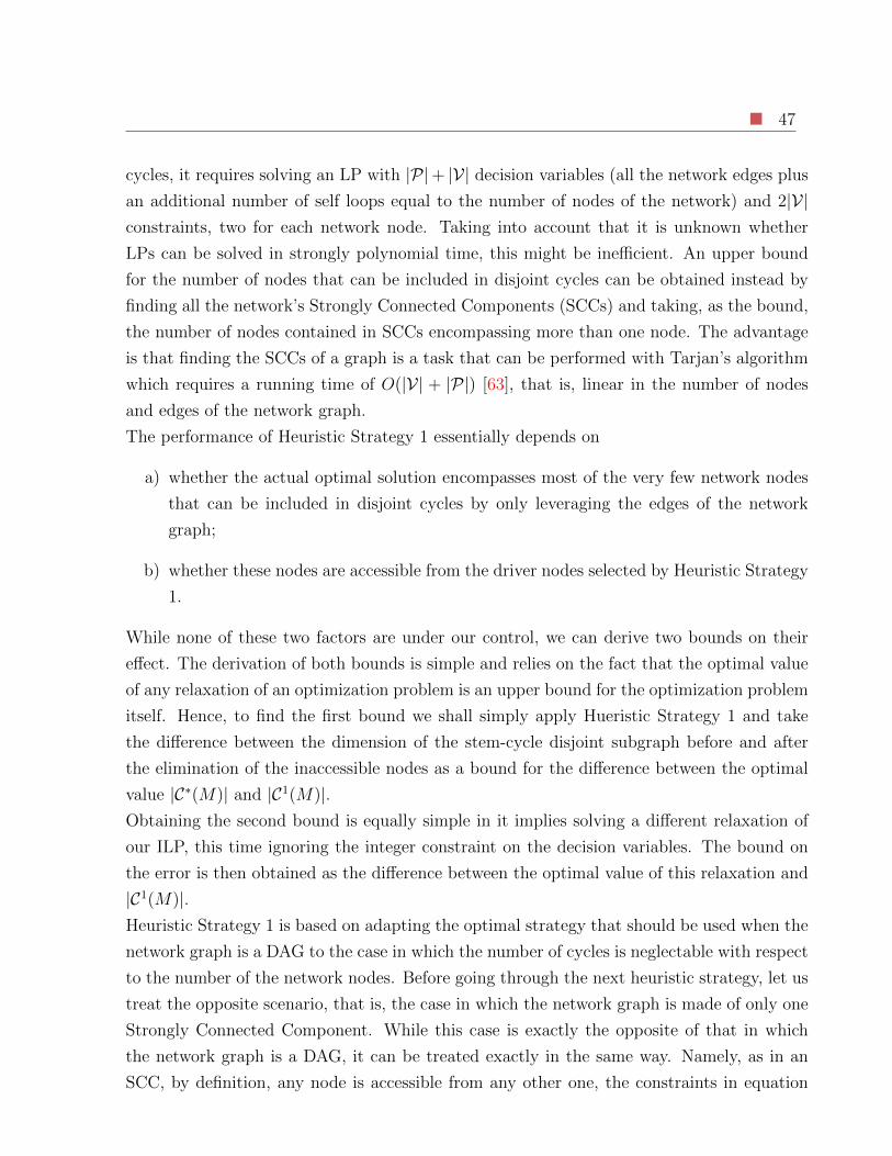
47
cycles, it requires solving an LP with |P|+ |V| decision variables (all the network edges plus
an additional number of self loops equal to the number of nodes of the network) and 2|V|constraints, two for each network node. Taking into account that it is unknown whether
LPs can be solved in strongly polynomial time, this might be inefficient. An upper bound
for the number of nodes that can be included in disjoint cycles can be obtained instead by
finding all the network’s Strongly Connected Components (SCCs) and taking, as the bound,
the number of nodes contained in SCCs encompassing more than one node. The advantage
is that finding the SCCs of a graph is a task that can be performed with Tarjan’s algorithm
which requires a running time of O(|V| + |P|) [63], that is, linear in the number of nodes
and edges of the network graph.
The performance of Heuristic Strategy 1 essentially depends on
a) whether the actual optimal solution encompasses most of the very few network nodes
that can be included in disjoint cycles by only leveraging the edges of the network
graph;
b) whether these nodes are accessible from the driver nodes selected by Heuristic Strategy
1.
While none of these two factors are under our control, we can derive two bounds on their
effect. The derivation of both bounds is simple and relies on the fact that the optimal value
of any relaxation of an optimization problem is an upper bound for the optimization problem
itself. Hence, to find the first bound we shall simply apply Hueristic Strategy 1 and take
the difference between the dimension of the stem-cycle disjoint subgraph before and after
the elimination of the inaccessible nodes as a bound for the difference between the optimal
value |C∗(M)| and |C1(M)|.Obtaining the second bound is equally simple in it implies solving a different relaxation of
our ILP, this time ignoring the integer constraint on the decision variables. The bound on
the error is then obtained as the difference between the optimal value of this relaxation and
|C1(M)|.Heuristic Strategy 1 is based on adapting the optimal strategy that should be used when the
network graph is a DAG to the case in which the number of cycles is neglectable with respect
to the number of the network nodes. Before going through the next heuristic strategy, let us
treat the opposite scenario, that is, the case in which the network graph is made of only one
Strongly Connected Component. While this case is exactly the opposite of that in which
the network graph is a DAG, it can be treated exactly in the same way. Namely, as in an
SCC, by definition, any node is accessible from any other one, the constraints in equation

48 5 Heuristic Driver Node Selection Strategies
(3-12) are redundant. Thus again thanks to the total unimodularity of the matrix defined
by equations (3-10) and (3-11) we can give the following Lemma.
Lemma 5.0.2. If the graph G is made of only one SCC, then the ILP in equations (3-8)-
(3-12) that must be solved in order to select a set of driver nodes of fixed cardinality M to
maximize the number of controllable nodes is not NP-hard.
Lemma 5.0.2 also applies to the case in which the network graph is made of a giant strongly
connected component plus an arbitrary number of one-node SCCs without self loops in the
upstream of the giant component. In this case, as the giant component is the only SCC
encompassing disjoint cycles, and as all of its nodes are accessible from all the network
nodes, the accessibility constraints in equation (3-12) are still redundant.
After having treated the two opposite scenarios of network graphs that are either DAGs
or made of one SCC together with two scenarios in which the network topology is close to
fulfilling one of these two conditions, let us turn our attention to the general case in which
the network graph is made of several SCCs each of at least two nodes and thus encompassing
cycles. As anticipated, in this case the idea is to decouple the accessibility problem from
that of finding an optimal cycle partition of a graph, that is, the two tasks performed by the
ILP in equations (3-8)-(3-12).
Heuristic Strategy 2: If the network graph is made of several SCCs each with more than two
nodes, then a good heuristic strategy is to place at least a fraction of the M driver nodes in
the Root Strongly Connected Components that have the largest number of nodes in disjoint
cycles in their downstream.
Deploying Heuristic Strategy 2 is not as straightforward as deploying Heuristic Strategy 1,
and thus we will now go through the details of its steps. The general idea is that when M is
small and the network is cycle rich then the relevance of the cycles in the largest stem-cycle
disjoint subgraph originating from the driver nodes (Γc) is much larger than that of the M
stems. Hence, placing the driver nodes in the RSCCs that have a large number of cycles in
their downstream ensures the heuristic strategy defines a large stem-cycle disjoint subgraph
Γc as its dimension will be at least equals to the number of nodes in these cycles. Before
giving the algorithm required to deploy Heuristic Strategy 2 we must define the following
notation:
• we denote by S = si the set of SCCs of a graph.
• we denote by R = ri ⊂ S the set of RSCCs of a graph.

49
• we denote by |si| the maximum number of nodes of the SCC si that can be included
into disjoint cycles;
• we denote by ∆(ri) the set of SCCs in the downstream of the RSCC ri, including ri.
• we denote by |∆(ri)| the maximum number of nodes of the SCCs in ∆(ri) that can be
included in disjoint cycles.
Algorithm 2
1. Find the set S of the SCCs of the network graph.
2. ∀ si ∈ S, find the maximum number of nodes of si that can be included in disjoint
cycles (|si|). We remark that this can be done by deploying Algorithm 1 skipping steps
2 − 7 and ignoring the constraint in equation (3-12) in the ILP (which can thus be
relaxed to a Linear Program).
3. ∀ ri ∈ R, find the maximum number of nodes in its downstream that can be included
in disjoint cycles (|∆(ri)|). We underline that |∆(ri)| =∑
j:sj∈∆(ri)|sj|, that is |∆(ri)|
is equal to the sum of the |sj| for all the SCCs sj that are in the downstream of the
RSCC ri.
4. Define the set D = ∅.
5. Define the set R = R− ∪i:|∆(ri)=0|(ri). The set R includes all the elements of R with
at least a cycle in their downstream.
6. Select, out of the set R, the RSCC r∗ = arg maxri∈R(|∆(ri)|).
7. Add r∗ to the set D.
8. Remove r∗ from the set R, that is, R = R− r∗.
9. Remove, from all the sets ∆(ri) : ri ∈ R, all the SCCs si that are in the downstream
of r∗.
10. Recompute |∆(ri)| for all ri ∈ R as
|∆(ri)| =∑
j:sj∈∆(ri)
|sj|. (5-1)
11. remove, from the set R all the elements ri such that |∆(ri)| = 0

50 5 Heuristic Driver Node Selection Strategies
12. repeat steps 6 to 10 until the number of elements in D is equal to M , that is, the
constraint on the number of driver nodes or until the set R is empty.
13. G ′ = G.
14. Remove from G ′ all the nodes that are not either i. nodes of the RSCCs in the set D
or ii. in the downstream of the RSCCs in the set D.
15. Define the scalar N = |V ′|. N is equal to the number of nodes of the graph G ′.
16. Find the set Ω′ = ∪i|vi∈vi∈rj∈D.
17. Add, to G ′ a new node, say N + 1.
18. Add |Ω′| new edges exiting node N + 1 and entering each node of Ω′.
19. Add N new edges exiting each node of G ′ and entering node N + 1.
20. Add N self loops, one for each node of G ′ except for node N + 1.
21. Associate a binary decision variable yij to each edge p′ij of G ′.
22. Associate a unit weight wij to each decision variable yij that is either:
• associated with an edge p′ij of G ′ that is also an edge of G;
• associated with an edge p′ij of G ′ that exits node N + 1;
23. Associate zero weight w′ij to all the other decision variables yij:
24. Solve the following Linear Program:
maxy
∑i
∑j
w′ijyij (5-2)
subject to
yij ∈ [0, 1] ∀i, j|p′ij ∈ P ′ (5-3)∑j
yij = 1 ∀i = 1, ..., N (5-4)∑i
yij = 1 ∀j = 1, ..., N (5-5)∑i:vi∈dj
yi,N+1 = 1 ∀j = 1, ...,M (5-6)

51
While Algorithm 2 is very lengthy, Heuristic Strategy 2 is actually very simple. As antici-
pated, the rationale is that selecting as a driver a node in an SCC si or in its upstream allows
controlling at least a number of nodes equal to |si| as all the cycles of si will be accessible
from the selected driver node. Hence, one would ideally want to select as drivers the nodes
that are encompassed in cycle rich SCCs but most importantly in SCCs that have cycle rich
downstreams. So the question shifts to which SCCs have the richest downstream in terms
of nodes that can be included in disjoint cycles. To answer this question, we can rely on
the DAG condensation of the network graph. In this new acyclic graph, there is an edge
connecting SCC si to SCC sj if, in the graph of the network G, there exists a directed path
from the nodes of si to the nodes of sj. The source nodes of the condensed graph correspond
to the RSCCs of the graph G. An example of a model network and of its DAG condensation
is provided in Figures 5-1(a) and (b).
As any non root SCC is in the downstream of at least an RSCC, then the SCCs with the
richest downstream in terms of nodes that can be included in disjoint cycles are indeed the
RSCCs, or, equivalently, the source nodes of the DAG condensation of G. Hence, Heuristic
Strategy 2 will select as drivers only the nodes of the RSCCs of the graph G. Among these
RSCCs, those with the richest downstream will be privileged. To do so, (steps 1 and 2) we
first find the set S of all the SCCs of the network and for each si we compute the value |si|,that is the maximum number of nodes of the SCC si that can be included in disjoint cycles.
Then, in step 3, we isolate the set of RSCCs R and for each of its elements ri we compute
the maximum number of nodes of their downstream that can be included in disjoint cycles
|∆(ri)|. This can be done by simply adding up all the |sj| of the SCCs in the downstream
of each root ri. After having defined the sets D and R (steps 4 and 5), in step 6 we take
the RSCC r∗ that has the largest |∆(ri)| and add it to the set of RSCCs D out of which the
drivers will be selected. As one driver node per RSCC ri is sufficient to ensure controllability
of the nodes of the SCCs in the set ∆(ri), we must select M RSCCs to compose the set D
as only one driver node will be selected out of each element of D. To do so, once the first
element of D has been selected (step 7), in steps 8 we remove it from the set R. Then, in
step 9 we remove all of its downstream from all the sets ∆(ri) ri 6= r∗ and in step 10 we
update the values of |∆(ri)| ri 6= r∗. Finally, we select, out of the remainder of the RSCCs,
the one with the largest associated |∆(ri)|. This procedure is repeated until the set D is
composed of M elements or until the set R of the RSCCs which have at least a cycle in their
downstream is empty.
From a conceptual standpoint, this iterative procedure can be viewed as a problem on a new
graph composed of two levels: one including the RSCCs such that |∆(rj) 6= 0| and another

52 5 Heuristic Driver Node Selection Strategies
including the non root SCCs such that |si| 6= 0. In this new graph, we can only have edges
connecting RSCCs to non root SCCs. Namely, an edge will connect RSCC ri to SCC sj if sj
is in the downstream of ri. The problem on this new graph consists in selecting the RSCC
that has in its downstream the SCCs with the largest number of nodes that can be included
in disjoint cycles, updating the graph by eliminating the selected root, its downstream, and
if necessary all the roots that no longer have SCCs in their dowstream, and finally repeating
these two steps until either M RSCCs have been selected or the new graph is empty. The
reduced graph for the model network in Figure 5-1(a) is shown in Figure 5-1(c). The red
circles correspond to the RSCCs while the blue circles to the non root SCCs.
Having defined the setD of the RSCCs in which the driver nodes will fall implicitly defines the
set of nodes that will be accessible from the driver nodes. Namely, these can be obtained by
taking the nodes of the RSCCs in the set D together with all the nodes in their downstream.
The a priori knowledge of the nodes that will be accessible from the drivers allows us to
ignore the accessibility constraints of the ILP in Algorithm 1. These must be substituted by
an additional set of constraints, those in equation (5-6), that ensure a driver node is selected
in each of the RSCCs of the set D. This time, the set of constraints in equations (5-4)-(5-6)
defines a totally unimodular matrix as it fulfills the conditions given in ref [30]. Moreover,
as the constant terms are integers, the ILP in equations (5-7)-(5-6) is not NP-hard.
Once we have selected the RSCCs in which the drivers will fall, we must proceed to the
selection of these drivers and of the set of controllable nodes C. This is done in steps 13 to
24 by simply specifying Algorithm 1 to the case in which a driver node must fall in each
RSCC of the set M . Note that the a priori knowledge on the set of nodes that will be
accessible from the drivers not only ensures the ILP is not NP-hard but reduces the number
of decision variables and constraints of the optimization problem. This as all the nodes of
the graph G that are not accessible from the drivers will certainly not be controllable and
thus can be eliminated from the graph G ′ together with all their associated edges. Figure
5-1(d) shows the graph of the same model network in Figure 5-1(a). This time, the nodes
selected as drivers are highlighted in green while the nodes accessible from the drivers are
highlighted in yellow. The blue circles represent the nodes that are inaccessible from the
drivers and thus will not be included in the graph G ′.For the sake of simplicity and clarity Steps 13 to 24 refer to the case in which the number
of elements of D is equal to M and not all the nodes of the network that can be included in
disjoint cycles are in the downstream of the RSCCs where the driver nodes will fall. If instead
all the nodes of the network that can be included in disjoint cycles are in the downstream
of the RSCCs of the set D, we can revert to considering, in the graph G ′, the entire network
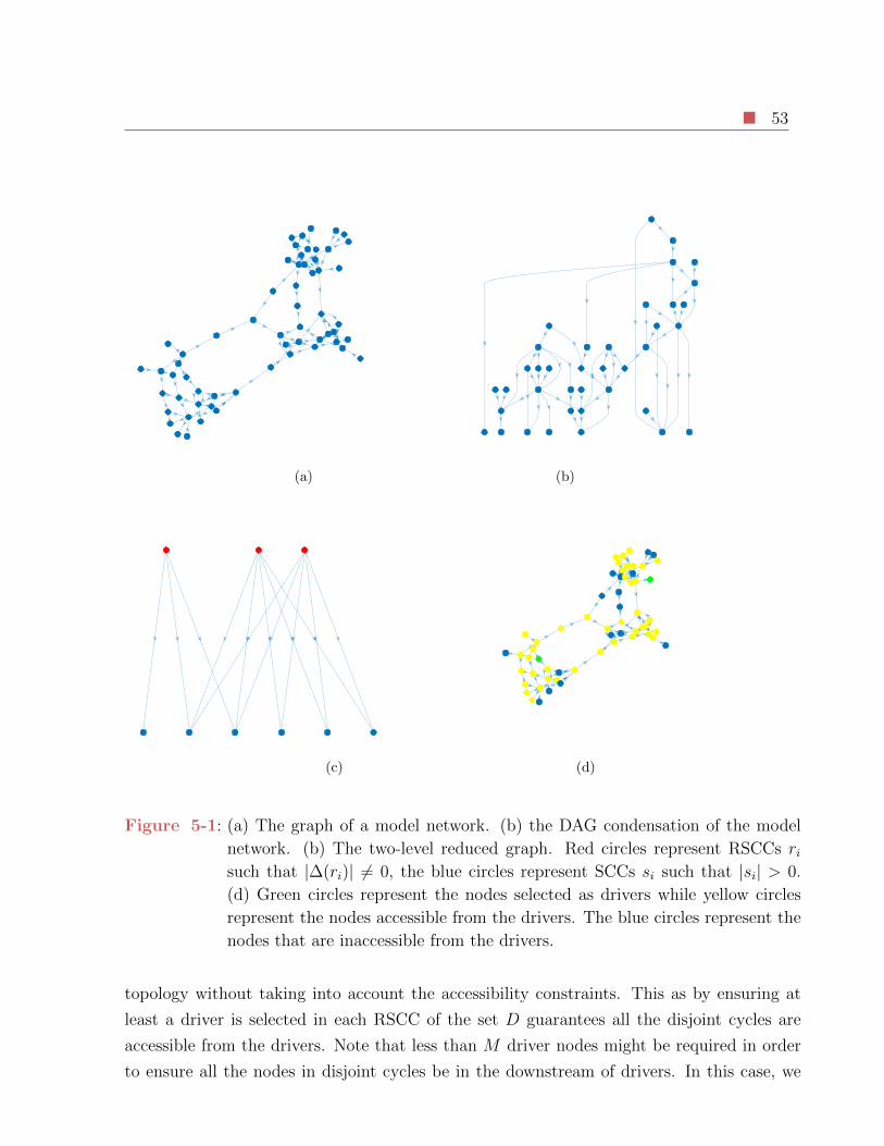
53
(a) (b)
(c) (d)
Figure 5-1: (a) The graph of a model network. (b) the DAG condensation of the model
network. (b) The two-level reduced graph. Red circles represent RSCCs risuch that |∆(ri)| 6= 0, the blue circles represent SCCs si such that |si| > 0.
(d) Green circles represent the nodes selected as drivers while yellow circles
represent the nodes accessible from the drivers. The blue circles represent the
nodes that are inaccessible from the drivers.
topology without taking into account the accessibility constraints. This as by ensuring at
least a driver is selected in each RSCC of the set D guarantees all the disjoint cycles are
accessible from the drivers. Note that less than M driver nodes might be required in order
to ensure all the nodes in disjoint cycles be in the downstream of drivers. In this case, we

54 5 Heuristic Driver Node Selection Strategies
will have that |D| < M and thus M − |D| driver nodes can be freely selected. To do so, we
take the set of |D| drivers, say ΩD, obtained after step 24 of Algorithm 2 and perform the
following steps in order to add |D| −M new drivers to the set ΩD.
25 G ′ = G.
26 Add, to G ′ a new node, say N + 1.
27 Add N new edges exiting node N + 1 and entering each node of G ′.
28 Add N new edges exiting each node of G ′ and entering node N + 1.
29 Add N self loops, one for each node of G ′ except for node N + 1.
30 Associate a binary decision variable yij to each edge p′ij of G ′.
31 Associate a unit weight wij to each decision variable yij that is either:
• associated with an edge p′ij of G ′ that is also an edge of G;
• associated with an edge p′ij of G ′ that exits node N + 1;
32 Associate zero weight w′ij to all the other decision variables yij:
33 Solve the following Linear Program:
maxy
∑i
∑j
w′ijyij (5-7)
subject to
yij ∈ [0, 1] ∀i, j|p′ij ∈ P ′ (5-8)∑j
yij = 1 ∀i = 1, ..., N (5-9)∑i
yij = 1 ∀j = 1, ..., N (5-10)∑j
yN+1,j = M (5-11)∑i:vi∈ΩD
yi,N+1 = |D| (5-12)
∑i:vi /∈ΩD
yi,N+1 = M − |D| (5-13)
Equations (5-12) and (5-13) of the ILP defined in step 33 ensure each node of ΩD is a driver
nodes that the other M − |D| drivers are freely selected out of the remainder of the network
nodes.

5.1 Performance Evaluation of Heuristic Strategy 2 55
5.1 Performance Evaluation of Heuristic Strategy 2
In the first part of this chapter, we have defined two heuristic strategies belonging to the
complexity class P able of coping with the problem of selecting M driver nodes in order to
maximize the number of controllable nodes of a network |C|. We showed that a priori, a
lower bound for the performance of Heuristic strategy 1 can be computed given the number
of network nodes that can be included in disjoint cycles as this heuristic strategy simply
consist in finding the largest stem-cycle disjoint subgraph of the network graph and then
eliminating the cycles that are not accessible from the drivers. Hence, as we are given the
freedom of choosing which heuristic to use based on the network topology we are coping with,
we have all the elements to decide whether Heuristic Strategy 1 fits our needs. Namely, given
a network topology, the larger the number of nodes that can be included in disjoint cycles,
the larger the error we are implicitly accepting in deploying Heuristic Strategy 1.
Differently from the case of Heursitc Strategy 1, evaluating the performance of Heuristic
Strategy 2 is nontrivial. A posteriori, we can always evaluate the difference between the
heuristic solution and the solution obtained by deploying Algorithm 1 while solving the LP
relaxation of the optimization problem in equations (3-8)-(3-12). While on one hand this
procedure gives us an uncertainty interval on the optimal value |C∗(M)|, on the other hand
little can be said without deploying both the heuristic strategy and Algorithm 1 relaxing
the integer constraints of the ILP. Unfortunately, this can be a very lengthy procedure. It is
thus interesting to perform a numerical analysis in order to compare the results of Heuristic
Strategy 2 to that of Algorithm 1. In this numerical analysis we aimed at considering
networks with different topological features so to provide a clear picture of the performance
of our the proposed heuristic. We start our numerical analysis by considering the topology
of the Cora citation Network [60, 17]. The topological features of this network are resumed
in Table 5-1.
|V| 23166
|P| 91500
|S| 18061
|R| 9396
Table 5-1: Main topological features of the Cora citation Network
This network is characterized by a reasonably large number of SCCs compared to the number
of network nodes. Nevertheless, of these 18061 SCCs one is a giant component made of 3991
nodes, the second largest being made of only 19 nodes. For this network, the maximum
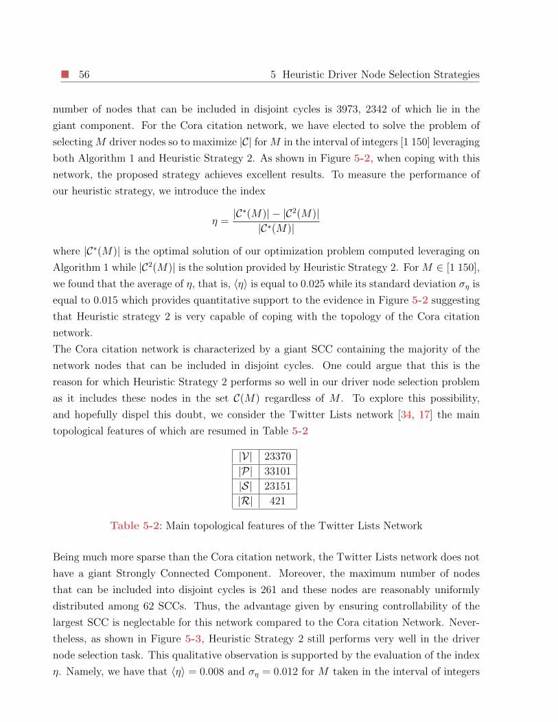
56 5 Heuristic Driver Node Selection Strategies
number of nodes that can be included in disjoint cycles is 3973, 2342 of which lie in the
giant component. For the Cora citation network, we have elected to solve the problem of
selecting M driver nodes so to maximize |C| for M in the interval of integers [1 150] leveraging
both Algorithm 1 and Heuristic Strategy 2. As shown in Figure 5-2, when coping with this
network, the proposed strategy achieves excellent results. To measure the performance of
our heuristic strategy, we introduce the index
η =|C∗(M)| − |C2(M)|
|C∗(M)|
where |C∗(M)| is the optimal solution of our optimization problem computed leveraging on
Algorithm 1 while |C2(M)| is the solution provided by Heuristic Strategy 2. For M ∈ [1 150],
we found that the average of η, that is, 〈η〉 is equal to 0.025 while its standard deviation ση is
equal to 0.015 which provides quantitative support to the evidence in Figure 5-2 suggesting
that Heuristic strategy 2 is very capable of coping with the topology of the Cora citation
network.
The Cora citation network is characterized by a giant SCC containing the majority of the
network nodes that can be included in disjoint cycles. One could argue that this is the
reason for which Heuristic Strategy 2 performs so well in our driver node selection problem
as it includes these nodes in the set C(M) regardless of M . To explore this possibility,
and hopefully dispel this doubt, we consider the Twitter Lists network [34, 17] the main
topological features of which are resumed in Table 5-2
|V| 23370
|P| 33101
|S| 23151
|R| 421
Table 5-2: Main topological features of the Twitter Lists Network
Being much more sparse than the Cora citation network, the Twitter Lists network does not
have a giant Strongly Connected Component. Moreover, the maximum number of nodes
that can be included into disjoint cycles is 261 and these nodes are reasonably uniformly
distributed among 62 SCCs. Thus, the advantage given by ensuring controllability of the
largest SCC is neglectable for this network compared to the Cora citation Network. Never-
theless, as shown in Figure 5-3, Heuristic Strategy 2 still performs very well in the driver
node selection task. This qualitative observation is supported by the evaluation of the index
η. Namely, we have that 〈η〉 = 0.008 and ση = 0.012 for M taken in the interval of integers
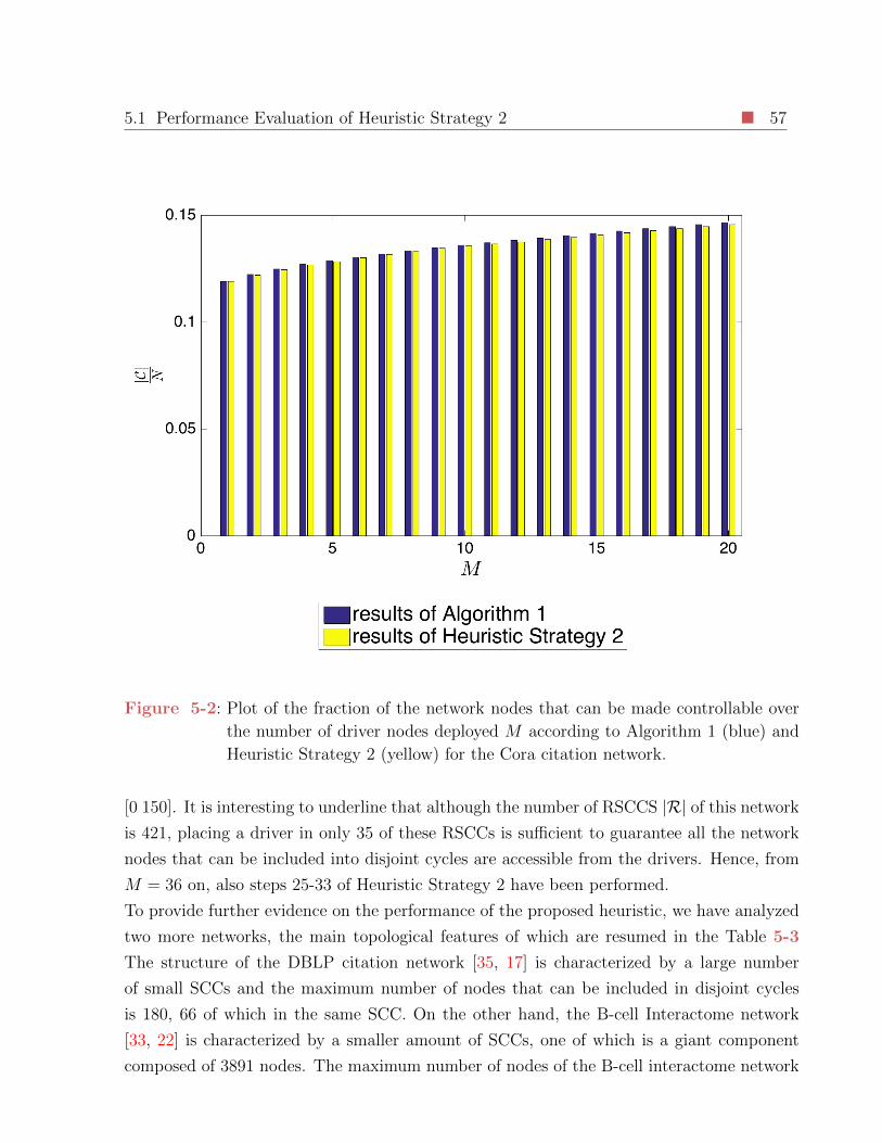
5.1 Performance Evaluation of Heuristic Strategy 2 57
Figure 5-2: Plot of the fraction of the network nodes that can be made controllable over
the number of driver nodes deployed M according to Algorithm 1 (blue) and
Heuristic Strategy 2 (yellow) for the Cora citation network.
[0 150]. It is interesting to underline that although the number of RSCCS |R| of this network
is 421, placing a driver in only 35 of these RSCCs is sufficient to guarantee all the network
nodes that can be included into disjoint cycles are accessible from the drivers. Hence, from
M = 36 on, also steps 25-33 of Heuristic Strategy 2 have been performed.
To provide further evidence on the performance of the proposed heuristic, we have analyzed
two more networks, the main topological features of which are resumed in the Table 5-3
The structure of the DBLP citation network [35, 17] is characterized by a large number
of small SCCs and the maximum number of nodes that can be included in disjoint cycles
is 180, 66 of which in the same SCC. On the other hand, the B-cell Interactome network
[33, 22] is characterized by a smaller amount of SCCs, one of which is a giant component
composed of 3891 nodes. The maximum number of nodes of the B-cell interactome network
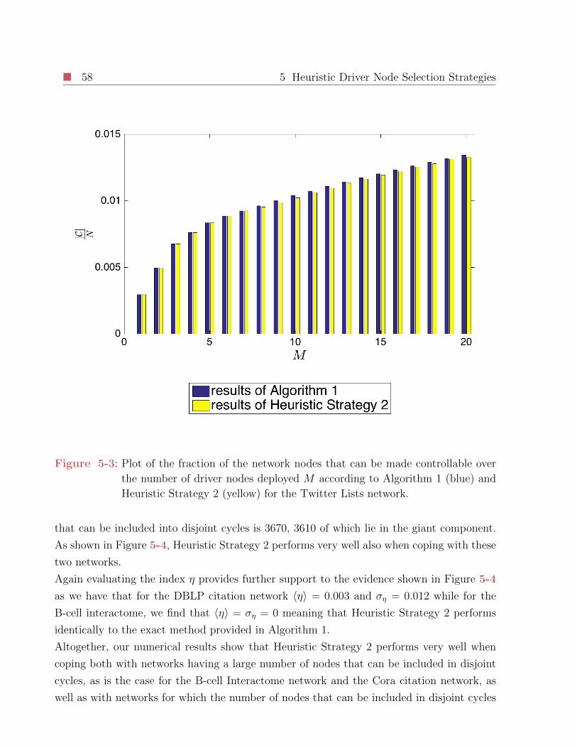
58 5 Heuristic Driver Node Selection Strategies
Figure 5-3: Plot of the fraction of the network nodes that can be made controllable over
the number of driver nodes deployed M according to Algorithm 1 (blue) and
Heuristic Strategy 2 (yellow) for the Twitter Lists network.
that can be included into disjoint cycles is 3670, 3610 of which lie in the giant component.
As shown in Figure 5-4, Heuristic Strategy 2 performs very well also when coping with these
two networks.
Again evaluating the index η provides further support to the evidence shown in Figure 5-4
as we have that for the DBLP citation network 〈η〉 = 0.003 and ση = 0.012 while for the
B-cell interactome, we find that 〈η〉 = ση = 0 meaning that Heuristic Strategy 2 performs
identically to the exact method provided in Algorithm 1.
Altogether, our numerical results show that Heuristic Strategy 2 performs very well when
coping both with networks having a large number of nodes that can be included in disjoint
cycles, as is the case for the B-cell Interactome network and the Cora citation network, as
well as with networks for which the number of nodes that can be included in disjoint cycles
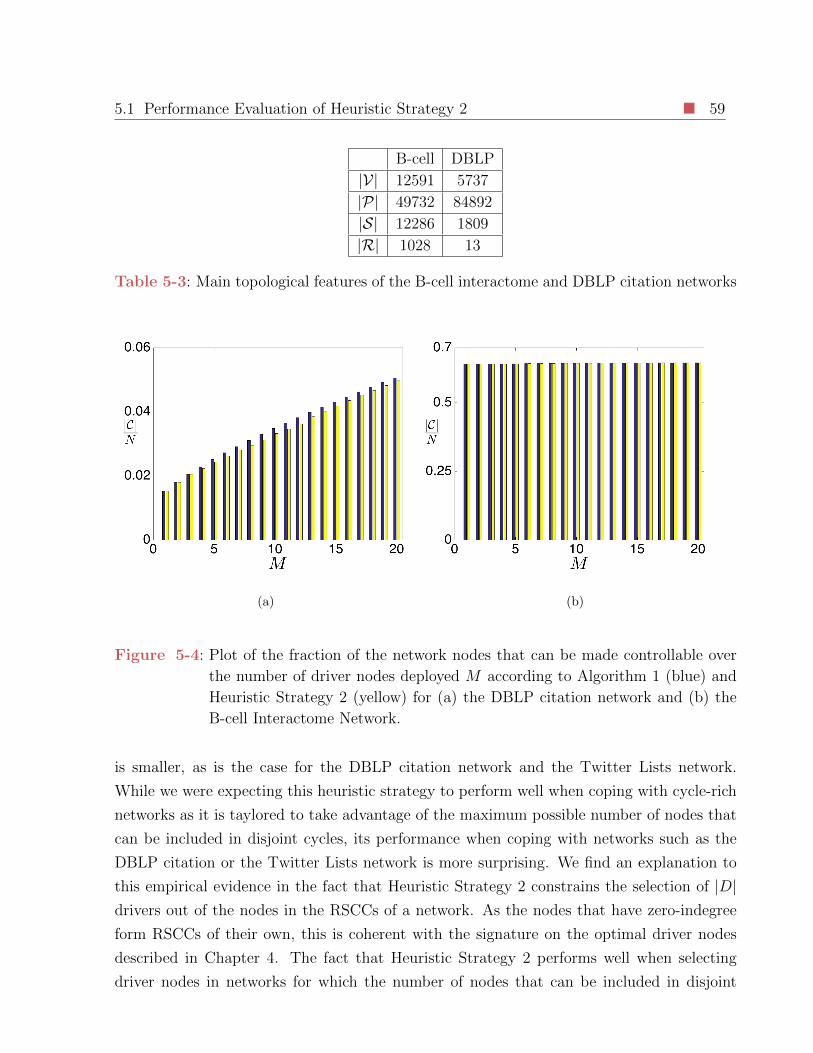
5.1 Performance Evaluation of Heuristic Strategy 2 59
B-cell DBLP
|V| 12591 5737
|P| 49732 84892
|S| 12286 1809
|R| 1028 13
Table 5-3: Main topological features of the B-cell interactome and DBLP citation networks
(a) (b)
Figure 5-4: Plot of the fraction of the network nodes that can be made controllable over
the number of driver nodes deployed M according to Algorithm 1 (blue) and
Heuristic Strategy 2 (yellow) for (a) the DBLP citation network and (b) the
B-cell Interactome Network.
is smaller, as is the case for the DBLP citation network and the Twitter Lists network.
While we were expecting this heuristic strategy to perform well when coping with cycle-rich
networks as it is taylored to take advantage of the maximum possible number of nodes that
can be included in disjoint cycles, its performance when coping with networks such as the
DBLP citation or the Twitter Lists network is more surprising. We find an explanation to
this empirical evidence in the fact that Heuristic Strategy 2 constrains the selection of |D|drivers out of the nodes in the RSCCs of a network. As the nodes that have zero-indegree
form RSCCs of their own, this is coherent with the signature on the optimal driver nodes
described in Chapter 4. The fact that Heuristic Strategy 2 performs well when selecting
driver nodes in networks for which the number of nodes that can be included in disjoint

60 5 Heuristic Driver Node Selection Strategies
cycles is not so large is encouraging as it fills the gap with Heuristic Strategy 1 which is
expected to perform well only when the number of nodes in disjoint cycles is small. This
ensures we have at our disposal a set of heuristic strategies that is expected to perform well
regardless of the network topology.
CHAPTER 6
Partial Observability of Complex
Networks
6.1 Observability of Dynamical Systems
According to the classical theory, a dynamical system is observable in a time interval [t0 tf ]
iff for all possible inputs and corresponding outputs it is possible to reconstruct its state
its state in finite time [5]. As it is well known, observability and controllability are dual
concepts. This implies that the controllability properties of a linear time invariant system
x = Fx+Bu (6-1)
y = Cx+Du
can be deduced by studying the observability properties of its dual representation
− x = −F Tx− CTu (6-2)
y = BTx+DTu.
More formally, this means that the controllable subspace of the linear system in equation
(6-1) is also the orthogonal complement of the unobservable subspace of its dual system in
equation (6-2). The duality between controllability and observability has several practical
implications. For instance, Kalman’s rank test for controllability of the system in (6-2)
provides the dimension of the observable subspace of the system in equation (6-1). It is for
this reason that we compute the dimension of the observable subspace as the rank of the
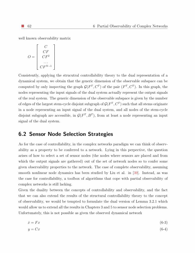
62 6 Partial Observability of Complex Networks
well known observability matrix
O =
C
CF
CF 2
. . .
CFN−1
Consistently, applying the strucutral controllability theory to the dual representation of a
dynamical system, we obtain that the generic dimension of the observable subspace can be
computed by only inspecting the graph G(F T , CT ) of the pair (F T , CT ). In this graph, the
nodes representing the input signals of the dual system actually represent the output signals
of the real system. The generic dimension of the observable subspace is given by the number
of edges of the largest stem-cycle disjoint subgraph of G(F T , CT ) such that all stems originate
in a node representing an input signal of the dual system, and all nodes of the stem-cycle
disjoint subgraph are accessible, in G(F T , BT ), from at least a node representing an input
signal of the dual system.
6.2 Sensor Node Selection Strategies
As for the case of controllability, in the complex networks paradigm we can think of observ-
ability as a property to be conferred to a network. Lying in this perpective, the question
arises of how to select a set of sensor nodes (the nodes where sensors are placed and from
which the output signals are gathered) out of the set of network nodes so to confer some
given observability properties to the network. The case of complete observability, assuming
smooth nonlinear node dynamics has been studied by Liu et al. in [39]. Instead, as was
the case for controllability, a toolbox of algorithms that cope with partial observability of
complex networks is still lacking.
Given the duality between the concepts of controllability and observability, and the fact
that we can also extend the results of the structural controllability theory to the concept
of observability, we would be tempted to formulate the dual version of Lemma 3.2.1 which
would allow us to extend all the results in Chapters 3 and 5 to sensor node selection problems.
Unfortunately, this is not possible as given the observed dynamical network
x = Fx (6-3)
y = Cx (6-4)
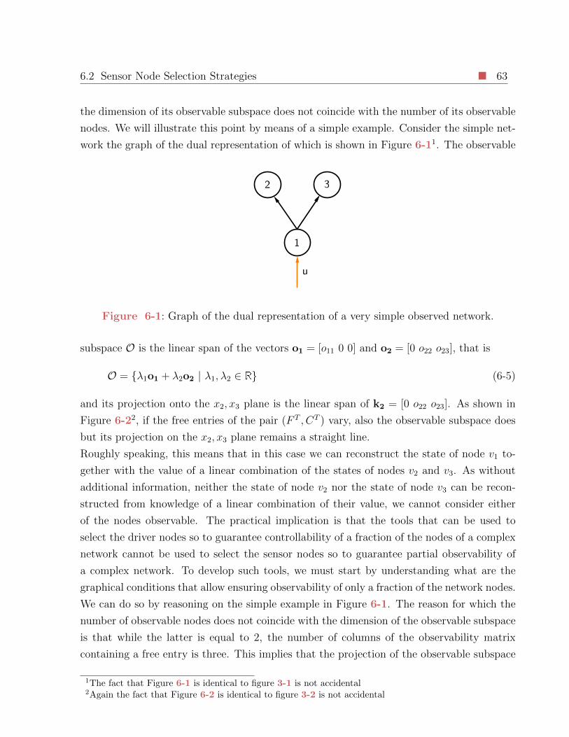
6.2 Sensor Node Selection Strategies 63
the dimension of its observable subspace does not coincide with the number of its observable
nodes. We will illustrate this point by means of a simple example. Consider the simple net-
work the graph of the dual representation of which is shown in Figure 6-11. The observable
Figure 6-1: Graph of the dual representation of a very simple observed network.
subspace O is the linear span of the vectors o1 = [o11 0 0] and o2 = [0 o22 o23], that is
O = λ1o1 + λ2o2 | λ1, λ2 ∈ R (6-5)
and its projection onto the x2, x3 plane is the linear span of k2 = [0 o22 o23]. As shown in
Figure 6-22, if the free entries of the pair (F T , CT ) vary, also the observable subspace does
but its projection on the x2, x3 plane remains a straight line.
Roughly speaking, this means that in this case we can reconstruct the state of node v1 to-
gether with the value of a linear combination of the states of nodes v2 and v3. As without
additional information, neither the state of node v2 nor the state of node v3 can be recon-
structed from knowledge of a linear combination of their value, we cannot consider either
of the nodes observable. The practical implication is that the tools that can be used to
select the driver nodes so to guarantee controllability of a fraction of the nodes of a complex
network cannot be used to select the sensor nodes so to guarantee partial observability of
a complex network. To develop such tools, we must start by understanding what are the
graphical conditions that allow ensuring observability of only a fraction of the network nodes.
We can do so by reasoning on the simple example in Figure 6-1. The reason for which the
number of observable nodes does not coincide with the dimension of the observable subspace
is that while the latter is equal to 2, the number of columns of the observability matrix
containing a free entry is three. This implies that the projection of the observable subspace
1The fact that Figure 6-1 is identical to figure 3-1 is not accidental2Again the fact that Figure 6-2 is identical to figure 3-2 is not accidental
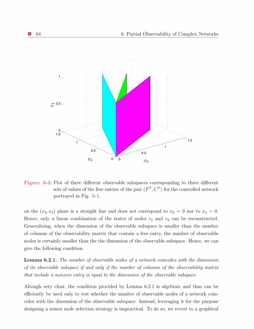
64 6 Partial Observability of Complex Networks
Figure 6-2: Plot of three different observable subspaces corresponding to three different
sets of values of the free entries of the pair (F T , CT ) for the controlled network
portrayed in Fig. 3-1.
on the (x2, x3) plane is a straight line and does not correspond to x2 = 0 nor to x3 = 0.
Hence, only a linear combination of the states of nodes v2 and v3 can be reconstructed.
Generalizing, when the dimension of the observable subspace is smaller than the number
of columns of the observability matrix that contain a free entry, the number of observable
nodes is certainly smaller than the the dimension of the observable subspace. Hence, we can
give the following condition
Lemma 6.2.1. The number of observable nodes of a network coincides with the dimension
of its observable subspace if and only if the number of columns of the observability matrix
that include a nonzero entry is equal to the dimension of the observable subspace.
Altough very clear, the condition provided by Lemma 6.2.1 is algebraic and thus can be
efficiently be used only to test whether the number of observable nodes of a network coin-
cides with the dimension of the observable subspace. Instead, leveraging it for the purpose
designing a sensor node selection strategy is impractical. To do so, we revert to a graphical

6.2 Sensor Node Selection Strategies 65
approach and consider the observed network
x = Ax (6-6)
y = Cx (6-7)
where once again, A is an adjacency matrix and each of its unit entries indicates a free entry
in the matrix F in equation (6-3). As usual, we will denote by G the graph defined by the
matrix A. Moreover, we also define the dual of the dynamical network in equation (6-6) as
−x = ATx− CTu (6-8)
and we denote by GT the graph defined by the matrix AT . As in this chapter we are interested
in optimizing the observability properties of a network, we will name sensor nodes both the
nodes of the network in equation (6-6) where the sensors are placed as well as the nodes of
the dual network in equation (6-8) where the input signals u are injected.
Now, we can give the graphical condition equivalent to Lemma 6.2.1.
Lemma 6.2.2. Consider the subgraph GTs of the graph GT of the dual network in equation
(6-8) composed of the nodes in the downstream of the sensor nodes and of all their connecting
edges. The number of observable nodes of the network in equation (6-6) coincides with the
dimension of its observable subspace if and only if there exists a stem-cycle disjoint subgraph
of GTs including all of its nodes and such that the source node of each stem is a sensor node.
Lemma 6.2.2 gives us a graphical condition to be verified that ensures a set of the network
nodes is observable from a given set of sensor nodes. In what follows, we will leverage
Lemma 6.2.2 to design sensor node selection strategies. The problem we will cope with is
that of selecting, out of the entire set of network nodes, a set of sensor nodes that guarantee
observability of the set controllable nodes C of a controlled network. We will thus assume
that both the set ΩD and C have been determined. The reason for which we decide to
cope with this specific problem is twofold. First of all, in most applications where the
complex network paradigm is deployed, the dynamics are only approximately known. For
this reason, the robustness properties of feedback control strategies, where applicable, are
appealing. As feedback control strategies rely on knowledge of the system state, observability
of the controllable nodes is required, unless a sensor is placed on each of the latter. This
brings us to the second point: we choose to determine the controllable nodes first, as thanks
to the toolbox of algorithms developed in Chapters 3 and 5 this selection can be optimal (or
suboptimal).

66 6 Partial Observability of Complex Networks
Our sensor node selection stategy is built in two steps. First, we guarantee that all the
controllable nodes be in the upstream, in the graph G, of at least a sensor node. This is
done by determining the set of RSCCs of the graph GT of minimum cardinality that ensures
all the controllable nodes are accessible, in GT , from at least one of the selected RSCCs,
and then placing a sensor in at least a node of each of these RSCCs. Then, we take the
subgraph GTS of GT in the downstream of the selected sensor nodes and ensure it fulfills the
conditions defined in Lemma 6.2.2 by selecting an additional set of sensor nodes. The steps
required to deploy this sensor node selection strategy are described in the following algorithm.
Algorithm 3
1. Find the set of SCCs S of the graph GT .
2. Find the set of RSCCs R ⊂ S of the graph GT .
3. Find the set of non root SCCs S = S −R.
4. Remove, from the set S all the SCCs that do not encompass a controllable node.
5. Find the set R ⊂ R of RSCCs that encompass at least a controllable node.
6. Associate a binary variable xi to each element of R.
7. Associate a set of binary variables zij, j = 1, . . . , |R| to each element si of S. Namely,
a binary variable zij is defined if the SCC si is in the downstream of the RSCC rj.
8. Solve the following ILP:
min∑j
xj (6-9)
s.t.
zij − xj = 0 ∀i, ∀j : ∃zij (6-10)
−∑j
zij ≤ −1 ∀i (6-11)
xj = 1 ∀j : rj ∈ R (6-12)
9. G ′ = GT .
10. Remove, from G ′ all the nodes that are neither i. associated to an RSCC rj such that
xj = 1 or ii. in the downstream of an RSCC rj such that xj = 1;

6.2 Sensor Node Selection Strategies 67
11. Define the scalar N = |V ′|. N is equal to the number of nodes of the graph G ′ as of
step 10.
12. Add, to G ′ a new node, say N + 1.
13. Add N new edges exiting node N + 1 and entering each node of G ′.
14. Add N new edges exiting each node of G ′ and entering node N + 1.
15. Associate a binary decision variable yij to each edge p′ij of G ′.
16. Solve the following Integer Linear Program:
miny
∑i
yi,N+1 (6-13)
subject to
yij ∈ 0, 1 ∀i, j|p′ij ∈ P ′ (6-14)∑j
yij = 1 ∀i = 1, ..., N (6-15)∑i
yij = 1 ∀j = 1, ..., N (6-16)
−∑
i:vi∈rj :xj=1
yi,N+1 ≤ −1 ∀j : xj = 1 (6-17)
Again, while Algorithm 3 might seem convoluted, its rationale is very simple. In steps 1-5
we find all the SCCs that encompass a controllable node, and all the RSCCs of the graph
G(AT ). Then, in steps 6-8 we ensure each controllable node be in the downstream (in G(AT ))
of at least a sensor node. This is done by associating a variabile xj to each RSCC of GT ,
and a set of variables zij to each SCC si that encompasses at least a controllable node. The
existence of the variable zij implies that the SCC si is in the downstream of the RSCC rj.
Then by solving the ILP in equations (6-9)-(6-12), the minimal set of RSCCs that have all
the controllable nodes in their downstream is selected. Namely, if xi = 1 then the RSCC
ri will include a sensor node. Equation (6-9) ensures the selected set is minimal, equations
(6-10) and (6-11) guarantee all non root SCCs that encompass a controllable node be in the
downstream of a selected RSCC, and equation (6-12) makes sure that all the RSCCs that
encompass controllable nodes also include a sensor node.
Steps 1-5 can be viewed as the construction of a two level graph where all the RSCCs are
source nodes and thus constitute the first level of this new graph and all the SCCs are sink
nodes and thus constitute the second level. The ILP in equations (6-9)-(6-12) then selects

68 6 Partial Observability of Complex Networks
the minimal set of sources of this two-level graph such that i. all sink nodes associated to
SCCs of GT that encompass a controllabe node are in the downstream of a selected source
and ii. all the sources associated to RSCCs that encompass a controllable node are selcted.
Once we have ensured each controllable node is in the downstream (in GT ) of at least a
sensor node, we must ensure the downstream of the latters is stem-cycle disjoint with each
stem originating from a sensor node. This is done in steps 9-16 by adding an additional
set of sensor nodes. Namely, in step 9 and 10 we start building an augmented graph G ′ by
eliminating, from the graph GT , all the nodes that are not in the selected RSCCs or in their
downstream. Then, in steps 12-14 we add an additional node representing the sensors to be
placed, and connect it to all the nodes of G ′. In step 15, we associate a binary variable yij to
each edge of the augmented graph G ′ and finally in step 16 we find the minimal set of sensor
nodes such that the downstream of the RSCCs selected in step 8 is stem-cycle disjoint, with
each stem originating from a sensor node. As was the case in Algorithm 1, this is done by
finding a cycle partition of the graph G ′. This time, as implied by equation (6-13), we seek
for the cycle partition that minimizes the number of edges exiting from node N + 1. As if
yi,N+1 = 1 then node i is a sensor node, this means minimizing the number of additional
sensor nodes deployed.
6.3 Computational Considerations
As the reader can note, Algorithm 3 encompasses two ILPs. Given the considerations made
in chapter 3 a legitimate question to ask is whether these are NP-hard. Let us start from
the second ILP, that in equations (6-13)-(6-17). We note that all constant terms are integer
and that the matrix defined by the constraints is binary. Hence, we must only prove that
we can decompose it into two blocks I1 and I2 as prescribed by Lemma 2.2.1. We already
know that the constraints in equations (6-15) and (6-16) will fall into the same block, say
I1, as they are the usual constraints used to find a cycle partition. The matrix defined by
the constriaint in equation (6-17) can fall in either block. In any case, it will not violate
any of the prescriptions in Lemma 2.2.1 as the variables that appear in its expression do not
appear in the other constraints. Hence the ILP in equations (6-13)-(6-17) is not NP-hard.
Now, we can turn our attention to the first ILP, that in equations (6-9)-(6-12). Once more,
the known terms of the constraints are integer and the elements of the constraint matrix only
take the values of −1, 0, 1 and thus it is worthwile checking if the constraint matrix fulfills
the sufficient condition for total unimodularity given in Lemma 2.2.1. If we choose to include
the matrix defined by the constraint in equation (6-10) in block I1 and the matrix defined

6.3 Computational Considerations 69
by the constraints in equations (6-12) and (6-11) in block I2 we note that each variable zij
appears once in block I1 and once in block I2 with opposite sign and the same applies to
each variable xj. Hence, the matrix defined by the constraints in equations (6-10)-(6-12) can
be decomposed as prescribed by Lemma 2.2.1 and thus also the first ILP in Algorithm 3 is
not NP-hard guaranteeing that Algorithm 3 can be deployed in polynomial time.
CHAPTER 7
Conclusions
Real world complex systems are not built to be controlled. Power grids, biological networks,
financial markets and social networks have developed without taking into explicit account
the need to control them. Hence, to control them efficiently, an accurate selection of the
nodes where input signals must be injected is required. As anticipated, we can translate
this problem into a different concept of controllability: from a structural property that a
dynamical system can, or cannot have, to a feature that must be conferred to some or all the
network nodes. From a theoretical point of view, this poses a new challenge, as the classical
tools of control theory must be complemented with driver node selection algorithms. In
the last five years, researchers from the engineering and physics community have promptly
responded to this challenge, as the problem of ensuring complete controllability of complex
networks has been vastly studied. Several papers have been published on this topic on
some of the most prestigious scientific journals. Perhaps, the most popular approach has
been that of leveraging the structural controllability theory to develop driver node selection
strategies to ensure complete controllability of complex networks. With the toolobox of
algorithms presented in this thesis, we have generalized this approach to the more realistic
scenario in which controllability is sought of only a fraction of the network nodes. We have
translated this shift of perspective into two optimization problems, a first one in which a
set of driver nodes of fixed cardinality must is selected in order to maximize the number
of controllable nodes of a network, and a second one in which the minimal set of driver
nodes is sought that allows ensuring structural controllability of a well-defined subset of the
network nodes. In this thesis we have presented optimal and suboptimal but computationally
efficient driver node selection algorithms capable of coping with the presented optimization
problems. Then, leveraging these tools, we have studied the relation between the network
structure and its readiness to be controlled, ultimately developing an index, the structural
7.1 Open problems and Future Work 71
permeability of complex networks to control signals, capable of measuring the ease with
which a network can be made controllable regardless of the number of driver nodes deployed
for the task. Finally, we have complemented the driver node selection algorithms with sensor
node selection strategies in order to ensure being able to deploy feedback control strategies.
This thesis has the ambition of capping off the topic of structural controllability of complex
networks in it generalizes the approaches found in the literature which are mainly related
to ensuring complete controllablity. We close this thesis by providing the reader with an
outlook on the current lines of reasearch that are currently under investigation on the topic
of controllability of complex networks.
7.1 Open problems and Future Work
In an effort to come closer to actually controlling complex networks, recently, researchers have
started to focus on measuring the effort required to control complex dynamical networks.
Taking different approaches [62], [64] [48], different studies have found that the worst-case
effort required to achieve a control goal grows exponentially with the ratio between the
driver nodes and the number of nodes of the network. In some sense this is not surprising,
as what allows indirectly controlling a network node, that is, the edges that link it to other
nodes, also introduces a dependency of its dynamics with respect to that of the nodes to
which it is connected. The results in these papers seem to suggest that although theretically
possibile, it is inpractical to control a number of nodes that is significantly larger than the
number of drivers deployed for the task. The viewpoint taken in this thesis is that to control
a number of nodes that is significantly larger than the number of drivers with reasonable
energy, the latters must be selected explicitly taking into account the control goal to be
accomplished. The idea is that, varying the the selected set of drivers nodes also changes the
paths, that is, the sequence of edges edges, through which the control signals will permeate
through the network. These paths determine the dependecies that will arise between the
controlled dynamics of the network nodes. Roughly speaking, we can imagine driver node
selection strategies that aim at exploiting the dependecies introduced by the network edges
that facilitate achieving the desired control goals while avoiding the selection, as drivers, of
the nodes that would make sure some undesired dependecies come into play. Indeed, this
can be a promising line of research that allows us to design driver node selection strategies
that can bring us close to actually controlling real world complex systems.

Bibliography
[1] Marian Anghel, Kenneth A Werley, and Adilson E Motter. Stochastic model for power
grid dynamics. In System Sciences, 2007. HICSS 2007. 40th Annual Hawaii Interna-
tional Conference on, pages 113–113. IEEE, 2007.
[2] Alex Arenas, Albert Dıaz-Guilera, Jurgen Kurths, Yamir Moreno, and Changsong Zhou.
Synchronization in complex networks. Physics Reports, 469(3):93–153, 2008.
[3] Albert-Laszlo Barabasi et al. Scale-free networks: a decade and beyond. science,
325(5939):412, 2009.
[4] Dongbo Bu, Yi Zhao, Lun Cai, Hong Xue, Xiaopeng Zhu, Hongchao Lu, Jingfen Zhang,
Shiwei Sun, Lunjiang Ling, Nan Zhang, et al. Topological structure analysis of the
protein–protein interaction network in budding yeast. Nucleic acids research, 31:2443–
2450, 2003.
[5] Frank M Callier and Charles A Desoer. Linear Systems Theory. Springer, 1991.
[6] Fei Chen, Zengqiang Chen, Linying Xiang, Zhongxin Liu, and Zhuzhi Yuan. Reaching
a consensus via pinning control. Automatica, 45(5):1215–1220, 2009.
[7] FG Commoner. A sufficient condition for a matrix to be totally unimodular. Networks,
3(4):351–365, 1973.
[8] Pietro DeLellis, Franco Garofalo, Francesco Lo Iudice, and Elena Napoletano. Wealth
distribution across communities of adaptive financial agents. New Journal of Physics,
17(8):083003, 2015.
[9] Pietro DeLellis, Franco Garofalo, Francesco Lo Iudice, and Giovanni Mancini. Decen-
tralised coordination of a multi-agent system based on intermittent data. International
Journal of Control, 88(8):1523–1532, 2015.

Bibliography 73
[10] Giovanni Filatrella, Arne Hejde Nielsen, and Niels Falsig Pedersen. Analysis of a power
grid using a kuramoto-like model. The European Physical Journal B, 61(4):485–491,
2008.
[11] Prasanna Gai and Sujit Kapadia. Contagion in financial networks. In Proceedings of
the Royal Society of London A: Mathematical, Physical and Engineering Sciences, page
rspa20090410. The Royal Society, 2010.
[12] Marco Galbiati, Danilo Delpini, and Stefano Battiston. The power to control. Nature
Physics, 9(3):126–128, 2013.
[13] Jianxi Gao, Yang-Yu Liu, Raissa M D’Souza, and Albert-Laszlo Barabasi. Target control
of complex networks. Nature communications, 5, 2014.
[14] K.-I. Goh, B. Kahng, and D. Kim. Universal behavior of load distribution in scale-free
networks. Phys. Rev. Lett., 87:278701, Dec 2001.
[15] J. Silvio Gutkind. Regulation of mitogen-activated protein kinase signaling networks
by g protein-coupled receptors. Sci. STKE, 2000(40):re1, 2000.
[16] S. Hosoe. Determination of generic dimensions of controllable subspaces and its appli-
cation. Automatic Control, IEEE Transactions on, 25(6):1192–1196, Dec 1980.
[17] http://konect.uni koblenz.de/networks.
[18] http://moreno.ss.uci.edu.
[19] http://research.mssm.edu/maayan/datasets.
[20] http://toreopsahl.com/datasets/.
[21] http://vlado.fmf.uni lj.si/pub/networks/data/bio/foodweb/foodweb.htm. Pajek’s
dataset.
[22] http://wiki.c2b2.columbia.edu/califanolab.
[23] http://wws.weizmann.ac.il/mcb/UriAlon/download/collection-complex networks.
[24] http://www3.nd.edu/ networks/resources/metabolic/index.html. Barabasilab dataset
of metabolic networks.
[25] http://www.wormatlas.org.
74 Bibliography
[26] Ramon Ferrer i Cancho, Christiaan Janssen, and Ricard V Sole. Topology of technology
graphs: Small world patterns in electronic circuits. Physical Review E, 64(4):046119,
2001.
[27] R. Kalman. Mathematical description of linear dynamical systems. Journal of the
Society for Industrial and Applied Mathematics Series A Control, 1(2):152–192, 1963.
[28] Stuart A Kauffman. Metabolic stability and epigenesis in randomly constructed genetic
nets. Journal of theoretical biology, 22(3):437–467, 1969.
[29] Wesley K. Kroeze, Douglas J. Sheffler, and Bryan L. Roth. G-protein-coupled receptors
at a glance. Journal of Cell Science, 116(24):4867–4869, 2003.
[30] Harold William Kuhn, Albert William Tucker, and George Bernard Dantzig. Linear
inequalities and related systems. Number 38. Princeton university press, 1956.
[31] Aud Larsen, Jorun K Egge, Jens C Nejstgaard, Iole Di Capua, Runar Thyrhaug, Gunnar
Bratbak, and T Frede Thingstad. Contrasting response to nutrient manipulation in
arctic mesocosms are reproduced by a minimum microbial food web model. Limnology
and oceanography, 60(2):360–374, 2015.
[32] Ernest Bruce Lee and Lawrence Markus. Foundations of optimal control theory. Tech-
nical report, DTIC Document, 1967.
[33] Celine Lefebvre, Wei Keat Lim, Katia Basso, Riccardo Dalla Favera, and Andrea Cali-
fano. A context-specific network of protein-dna and protein-protein interactions reveals
new regulatory motifs in human b cells. In Systems Biology and Computational Pro-
teomics, pages 42–56. Springer, 2007.
[34] Jure Leskovec and Julian J Mcauley. Learning to discover social circles in ego networks.
In Advances in neural information processing systems, pages 539–547, 2012.
[35] Michael Ley. The dblp computer science bibliography: Evolution, research issues, per-
spectives. In String Processing and Information Retrieval, pages 1–10. Springer, 2002.
[36] Ching-Tai Lin. Structural controllability. Automatic Control, IEEE Transactions on,
19(3):201–208, Jun 1974.
[37] Yang-Yu Liu, Jean-Jacques Slotine, and Albert-Laszlo Barabasi. Controllability of com-
plex networks. Nature, 473(7346):167–173, 2011.
Bibliography 75
[38] Yang-Yu Liu, Jean-Jacques Slotine, and Albert-Laszlo Barabasi. Control centrality and
hierarchical structure in complex networks. PLoS ONE, 7(9):e44459, 09 2012.
[39] Yang-Yu Liu, Jean-Jacques Slotine, and Albert-Laszlo Barabasi. Observability of com-
plex systems. Proceedings of the National Academy of Sciences, 110(7):2460–2465, 2013.
[40] Francesco Lo Iudice, Franco Garofalo, and Francesco Sorrentino. On the observability
of the largest set of controllable nodes of complex networks. 2016.
[41] Thomas Lux and Michele Marchesi. Scaling and criticality in a stochastic multi-agent
model of a financial market. Nature, 397(6719):498–500, 1999.
[42] H Maeda, G Y Bharate, and J Daruwalla. Polymeric drugs for efficient tumor-targeted
drug delivery based on epr-effect. European Journal of Pharmaceutics and Biopharma-
ceutics, 71(3):409 – 419, 2009.
[43] Susanna C Manrubia, Alexander S Mikhailov, et al. Emergence of dynamical order:
synchronization phenomena in complex systems, volume 2. World Scientific, 2004.
[44] Maria Julia Marinissen and J Silvio Gutkind. G-protein-coupled receptors and signaling
networks: emerging paradigms. Trends in Pharmacological Sciences, 22(7):368 – 376,
2001.
[45] Marc Mezard and Giorgio Parisi. The bethe lattice spin glass revisited. The European
Physical Journal B-Condensed Matter and Complex Systems, 20(2):217–233, 2001.
[46] Tamas Nepusz and Tamas Vicsek. Controlling edge dynamics in complex networks.
Nature Physics, 8(7):568–573, 2012.
[47] R. Olfati-Saber. Flocking for multi-agent dynamical systems: algorithms and theory.
IEEE Trans. Autom. Contr., 51:401–419, 2006.
[48] Fabio Pasqualetti, Sandro Zampieri, and Francesco Bullo. Controllability metrics, limi-
tations and algorithms for complex networks. Control of Network Systems, IEEE Trans-
actions on, 1(1):40–52, 2014.
[49] S. Poljak. On the generic dimension of controllable subspaces. Automatic Control, IEEE
Transactions on, 35(3):367–369, Mar 1990.
[50] Maurizio Porfiri, D Gray Roberson, and Daniel J Stilwell. Tracking and formation
control of multiple autonomous agents: A two-level consensus approach. Automatica,
43(8):1318–1328, 2007.
76 Bibliography
[51] Wei Ren. Consensus strategies for cooperative control of vehicle formations. Control
Theory & Applications, IET, 1(2):505–512, 2007.
[52] Wei Ren and Randal W Beard. Distributed consensus in multi-vehicle cooperative con-
trol. Springer, 2008.
[53] Craig W Reynolds. Flocks, herds and schools: A distributed behavioral model. In ACM
SIGGRAPH computer graphics, volume 21, pages 25–34. ACM, 1987.
[54] Sara Brin Rosenthal, Colin R Twomey, Andrew T Hartnett, Hai Shan Wu, and Iain D
Couzin. Revealing the hidden networks of interaction in mobile animal groups allows
prediction of complex behavioral contagion. Proceedings of the National Academy of
Sciences, 112(15):4690–4695, 2015.
[55] Justin Ruths and Derek Ruths. Control profiles of complex networks. Science,
343(6177):1373–1376, 2014.
[56] Robert W Shields and J Boyd Pearson. Structural controllability of multi-input linear
systems. Rice University ECE Technical Report, (TR7502), 1975.
[57] Brian Skyrms and Robin Pemantle. A dynamic model of social network formation. In
Adaptive Networks, pages 231–251. Springer, 2009.
[58] Francesco Sorrentino, Mario di Bernardo, Franco Garofalo, and Guanrong Chen. Con-
trollability of complex networks via pinning. Phys. Rev. E, 75:046103, Apr 2007.
[59] Steven H Strogatz. Exploring complex networks. Nature, 410(6825):268–276, 2001.
[60] Lovro Subelj and Marko Bajec. Model of complex networks based on citation dynamics.
In Proceedings of the 22nd international conference on World Wide Web companion,
pages 527–530. International World Wide Web Conferences Steering Committee, 2013.
[61] Tyler Summers, Fabrizio Cortesi, and John Lygeros. On submodularity and controlla-
bility in complex dynamical networks. 2014.
[62] Jie Sun and Adilson E Motter. Controllability transition and nonlocality in network
control. Physical review letters, 110(20):208701, 2013.
[63] Robert Tarjan. Depth-first search and linear graph algorithms. SIAM journal on com-
puting, 1(2):146–160, 1972.

Bibliography 77
[64] Gang Yan, Georgios Tsekenis, Baruch Barzel, Jean-Jacques Slotine, Yang-Yu Liu, and
Albert-Laszlo Barabasi. Spectrum of controlling and observing complex networks. Na-
ture Physics, 11:779–786, 2015.
[65] Wenwu Yu, Guanrong Chen, Jinhu Lu, and Jurgen Kurths. Synchronization via pinning
control on general complex networks. SIAM Journal on Control and Optimization,
51(2):1395–1416, 2013.
[66] Zhengzhong Yuan, Chen Zhao, Zengru Di, Wen-Xu Wang, and Ying-Cheng Lai. Exact
controllability of complex networks. Nature communications, 4, 2013.
[67] Lenka Zdeborova and Marc Mezard. The number of matchings in random graphs.
Journal of Statistical Mechanics: Theory and Experiment, 2006(05):P05003, 2006.
[68] Ranran Zhang, Mithun Vinod Shah, Jun Yang, Susan B. Nyland, Xin Liu, Jong K.
Yun, Reka Albert, and Thomas P. Loughran. Network model of survival signaling in
large granular lymphocyte leukemia. Proceedings of the National Academy of Sciences,
105(42):16308–16313, 2008.


![LOGIC SENSOR PROOUT Gate Driver Providing Galvanic ... · LOGIC SENSOR PROOUT Gate Driver Providing Galvanic ... ... 4]]]](https://img.pdfslide.net/doc/110x75/5f97e95f3e31877b342a40b6/logic-sensor-proout-gate-driver-providing-galvanic-logic-sensor-proout-gate.jpg)