DROP TEST OF A SOFT BEVERAGE PACKAGE - Solid Mechanics

Department of Mechanical Engineering

Solid Mechanics

ISRN LUTFD2/TFHF-06/5122-SE(1-80)

DROP TEST OF A SOFT

BEVERAGE PACKAGE –

EXPERIMENTAL TESTS AND A

PARAMETER STUDY IN ABAQUS

Master’s Dissertation by

Johanna Lonnand

Jenny Navred

Supervisors

Eskil Andreasson, Tetra Pak R&D AB, SwedenHakan Hallberg, Div. of Solid Mechanics, Lund University, Sweden

Magnus Harrysson, Div. of Solid Mechanics, Lund University, Sweden

Copyright c© 2006 by Div. of Solid Mechanics,Tetra Pak R&D AB, Johanna Lonn, Jenny Navred

Printed by Media-Tryck, Lund University, Lund, SwedenFor information, adress:

Division of Solid Mechanics, Lund University, Box 118, SE-221 00 Lund, SwedenHomepage: http://www.solid.lth.se

Acknowledgement

The research presented in this master's thesis was carried out at Tetra PakR&D AB in Lund in cooperation with the Division of Solid Mechanics at theUniversity of Lund, Sweden, during October 2005 to March 2006.

At rst we would like to express our deepest gratitude to our supervisorM.Sc Eskil Andreasson at Tetra Pak R&D AB, for his support and guidancethroughout this project. Without his assistance and devotion this thesiswould have been dicult to complete.

Further a great thanks to our supervisors PhD students Magnus Harryssonand Håkan Hallberg at the Division of Solid Mechanics, for their help withthe theory and helpful ideas.

We would also like to thank the sta at Tetra Pak in Lund for valuableinput to the project and their help.

Lund, April 2006

Johanna Lönn and Jenny Navréd

i

ii ACKNOWLEDGEMENT

Abstract

Beverage packages are tested in many ways at Tetra Pak to determine theirproperties. In this master's thesis the drop test method will be considered.The goal is to evaluate the possibilities to perform FE-simulations of thedynamic drop test procedure. A wish is to establish a parameter that willpredict if the package can resist an impact from a desired height.

The FE-simulations will be performed in the computer software ABAQUS/Explicit since this program is suitable for dynamic impact problems. Threevarious modelling techniques have been tried out and a skin modelling methodwas selected. This method is easy to use and the best interaction betweenthe liquid product and the package was received. The FE-model in thesimulation is simplied to obtain a model that is easy to handle. Simpli-cations have been made on the transversal sealing and no initial folds havebeen introduced. The packaging material contains paperboard and therebythe laminate structure has orthotropic properties in the elastic and plas-tic area which will be assigned in the FE-model. The uid properties areassigned by an equation of state, EOS, to represent the uid behaviour inABAQUS/Explicit.

It has been detected that the failure in the package during a drop test oftenoccurs in the area of the transversal sealing. The test method that will beconsidered to evaluate the strength in the transversal sealings is the dynamicpendulum. Unfortunately no satisfying result was obtain from the pendu-lum setup used in this thesis and therefore the transversal sealings cannot beevaluated.

The main purpose with this thesis is accomplished since it is possible toFE-simulate a drop test procedure of a soft beverage package. The resultsthat are captured in the simulations are evaluated against each other andhigh-speed lms. The behaviour in the FE-simulations are similar betweenthe simulated drop heights. The high-speed lms indicate on the same be-

iii

iv ABSTRACT

haviour as the FE-simulations show. An interesting discovery is that shearstress concentrations are usually located in the same areas that cracks ap-pear in the packaging material. The MD stresses increase with the dropheight. This corresponds well to reality since more packages are damagedwhen dropped from higher heights. It is also established that the orientationof the package in a drop test highly aect the result of the test. This is de-termined by examine the reaction forces during impact in the FE-simulations.

Keywords: drop-test, FE-simulation, ABAQUS/Explicit, hardening mod-els, beverage packages.

Contents

Acknowledgement i

Abstract iii

1 Introduction 11.1 Background . . . . . . . . . . . . . . . . . . . . . . . . . . . . 11.2 Problem formulation . . . . . . . . . . . . . . . . . . . . . . . 11.3 Objectives . . . . . . . . . . . . . . . . . . . . . . . . . . . . . 21.4 Limitations and assumptions . . . . . . . . . . . . . . . . . . . 2

2 Package information 32.1 The packaging material . . . . . . . . . . . . . . . . . . . . . . 32.2 The packaging sealings . . . . . . . . . . . . . . . . . . . . . . 42.3 The product in the package . . . . . . . . . . . . . . . . . . . 4

3 Theory 73.1 Continuum mechanics . . . . . . . . . . . . . . . . . . . . . . 7

3.1.1 Kinematics of large deformations . . . . . . . . . . . . 73.1.2 Strain measures . . . . . . . . . . . . . . . . . . . . . . 83.1.3 Stress measures . . . . . . . . . . . . . . . . . . . . . . 9

3.2 Equation of motion . . . . . . . . . . . . . . . . . . . . . . . . 103.3 Constitutive model . . . . . . . . . . . . . . . . . . . . . . . . 12

3.3.1 Hill's orthotropic yield criterion . . . . . . . . . . . . . 123.3.2 Hardening models . . . . . . . . . . . . . . . . . . . . . 13

4 Numerical solution method 174.1 FE-formulation . . . . . . . . . . . . . . . . . . . . . . . . . . 174.2 Implicit vs explicit code formulation . . . . . . . . . . . . . . . 184.3 Explicit calculation method . . . . . . . . . . . . . . . . . . . 194.4 Energy balance . . . . . . . . . . . . . . . . . . . . . . . . . . 22

v

vi CONTENTS

5 Experimental test methods 235.1 Drop test . . . . . . . . . . . . . . . . . . . . . . . . . . . . . 23

5.1.1 Experimental setup . . . . . . . . . . . . . . . . . . . . 245.1.2 Result . . . . . . . . . . . . . . . . . . . . . . . . . . . 24

5.2 Dynamic pendulum . . . . . . . . . . . . . . . . . . . . . . . . 255.2.1 Experimental setup . . . . . . . . . . . . . . . . . . . . 265.2.2 Result . . . . . . . . . . . . . . . . . . . . . . . . . . . 27

5.3 Discussion . . . . . . . . . . . . . . . . . . . . . . . . . . . . . 27

6 Material models 296.1 Packaging material . . . . . . . . . . . . . . . . . . . . . . . . 29

6.1.1 Orthotropic elastic parameters . . . . . . . . . . . . . . 306.1.2 Orthotropic plastic parameters . . . . . . . . . . . . . 316.1.3 Verifying hardening models . . . . . . . . . . . . . . . 326.1.4 Conclusion . . . . . . . . . . . . . . . . . . . . . . . . . 35

6.2 Fluid material . . . . . . . . . . . . . . . . . . . . . . . . . . . 35

7 FE-modelling in ABAQUS 377.1 Modelling procedures . . . . . . . . . . . . . . . . . . . . . . . 38

7.1.1 Model with merged nodes . . . . . . . . . . . . . . . . 407.1.2 Model with skin . . . . . . . . . . . . . . . . . . . . . . 417.1.3 Choice of simulation model . . . . . . . . . . . . . . . . 417.1.4 Sealings in the FE-model . . . . . . . . . . . . . . . . . 42

7.2 Element types . . . . . . . . . . . . . . . . . . . . . . . . . . . 437.3 Assigning packaging material . . . . . . . . . . . . . . . . . . 447.4 Boundary conditions . . . . . . . . . . . . . . . . . . . . . . . 447.5 FE-simulations in ABAQUS/Explicit . . . . . . . . . . . . . . 457.6 Summary of the modelling procedure . . . . . . . . . . . . . . 46

8 Parameter variation and result 498.1 Horizontal fall . . . . . . . . . . . . . . . . . . . . . . . . . . . 49

8.1.1 Result . . . . . . . . . . . . . . . . . . . . . . . . . . . 508.2 Vertical fall . . . . . . . . . . . . . . . . . . . . . . . . . . . . 56

8.2.1 Result . . . . . . . . . . . . . . . . . . . . . . . . . . . 568.3 Longitudinal sealing . . . . . . . . . . . . . . . . . . . . . . . 57

8.3.1 Result . . . . . . . . . . . . . . . . . . . . . . . . . . . 578.4 Material . . . . . . . . . . . . . . . . . . . . . . . . . . . . . . 58

8.4.1 Result . . . . . . . . . . . . . . . . . . . . . . . . . . . 588.5 Mesh density . . . . . . . . . . . . . . . . . . . . . . . . . . . 58

8.5.1 Result . . . . . . . . . . . . . . . . . . . . . . . . . . . 58

CONTENTS vii

9 Discussion 619.1 Conclusion . . . . . . . . . . . . . . . . . . . . . . . . . . . . . 629.2 Further Work . . . . . . . . . . . . . . . . . . . . . . . . . . . 63

Bibliography 65

A Package modelled in ABAQUS 67

B Comparing FE-simulations with high-speed lm 71

C ABAQUS/Explicit input-le 75

viii CONTENTS

Chapter 1

Introduction

Tetra Pak is one of the big companies on the liquid carton based packagingmarket. All around the world beverages are packed in Tetra Pak packages.The product that will be studied in this master's thesis is a soft aseptic pouch.The challenge is to develop a package with acceptable properties even thoughthe packaging material is relatively thin.

1.1 BackgroundBeverage packages are tested in many ways to determine their properties.One way is to perform drop tests that give an approximated value of thedrop height for the package. This method has to be performed at a largenumber of packages to evaluate the ability of the packages to resist an impact.An interesting idea is to investigate whether it is possible to perform FiniteElement simulations, FE-simulations, of the drop test procedure. This wouldbring benets to the development time which could be reduced since theFE-simulation can provide essential information in the choice of packagingmaterial. A wish at Tetra Pak R&D regarding this thesis is to be able topredict a drop height that will not result in damaged packages.

1.2 Problem formulationThe main problem in this thesis is to investigate whether it is possible to FE-simulate with a nite element model, FE-model, a soft package containinga liquid product during impact. The FE-simulations will be performed inthe computer program ABAQUS/Explicit. The diculties are to solve thelarge deformations due to the uid and material properties. If this problemis solved the next step will be to investigate whether there is a parameter to

1

2 CHAPTER 1. INTRODUCTION

evaluate and compare against to detect dierences in packaging materials.This evaluation will be done in both FE-simulations and experimental tests.

1.3 ObjectivesThe primary goal of this thesis is to investigate the possibility to FE-simulatethe soft package during impact. The following goals are dened if the primarygoal is achieved. One of these goals is to determine a parameter that canbe used to predict the critical drop height of a packaging material. Anothergoal is to evaluate the FE-simulation possibilities with this type of model.

1.4 Limitations and assumptionsThe FE-simulation model will be simplied since the geometry and sealingsare complex. All folds and imperfections are eliminated in order to simplifythe modelling procedure. The packaging material will be considered as onematerial and not as a laminate structure. This limitation will shorten thesolution time. The milk product is simplied to water since the dierencesare assumed to be negligible.

Chapter 2

Package information

The shape of the package used in this thesis is the same as the already existingTFA pouch, Tetra Fino Aseptic. The volume of the package is 250 ml. Themanufacturing process of the package is simple and contains only a few steps.The package material is fed from a roll of material, according to Figure 2.1,and then the material is sterilized and nally formed to a tube. The tube islled with product and sealed in both ends. The idea of an aseptic packageis that it can be kept at room temperature without spoiling the product.

Figure 2.1: Manufacturing process of an aseptic pounch [1].

2.1 The packaging materialThe packaging material contains polymer and paperboard layers. To protectthe milk a polymer layer is used as a light barrier. When using paperboard aspackaging material it is important to be aware of the orthotropic properties.

3

4 CHAPTER 2. PACKAGE INFORMATION

Orthotropic behaviour means that the material has dierent properties inthe three directions according to Figure 2.2. The reason paperboard hasorthotropic behaviour is due to that the bers are oriented in the paperboardmanufacturing process. Primarily the bers are oriented in the plane wherethe machine direction, MD, is the dominating one. The other directions arethe cross machine direction, CD, and the out of plane direction, ZD.

MD

ZD

CD

Figure 2.2: Paperboard properties in dierent direction.

2.2 The packaging sealingsThere are dierent types of sealing techniques that are used in dierent typesof machine systems and materials, to achieve a desirable strength in thesealings. The package has two types of sealings, longitudinal and transversal,as presented in Figure 2.3. The longitudinal sealing is created by an overlapalong the sides when forming the tube in the lling process. To preventpenetration of liquid in the packaging material a polymer strip is placedover the longitudinal sealing. In the package impulse heating is used for thetransversal sealings. During the sealing process the tube is sealed and cutinto packages. Two jaws squeeze the tube together in intervals. In a squeezemotion the jaw seals the top of the lower package and the bottom in thepackage above the lower package as shown in Figure 2.1.

2.3 The product in the packageThe product in the package is as mentioned milk. To be more precise it isUHT, ultra heat treated, milk which means that the milk can be stored atroom temperature in a sterile package. The content in the package is water

2.3. THE PRODUCT IN THE PACKAGE 5

Figure 2.3: Longitudinal and transversal sealings in the package.

during the development process since milk is too expensive. The dierencesbetween milk and water are assumed to be negligible in this thesis since thedrop tests are performed with water.

6 CHAPTER 2. PACKAGE INFORMATION

Chapter 3

Theory

This chapter will cover the theory used in this thesis. The theory is neededin order to understand the deformation aspects and the choice of materialmodel. The theory that is described in this chapter is used in the com-putational solution program. The main topics that will be described arecontinuum mechanics, equation of motion and constitutive models.

3.1 Continuum mechanicsThis section covers the essential parts of continuum mechanics. At rst thebasic theory of large deformation is introduced followed by strain and stressmeasures. The equation of motion will then be reformulated to the principleof virtual power.

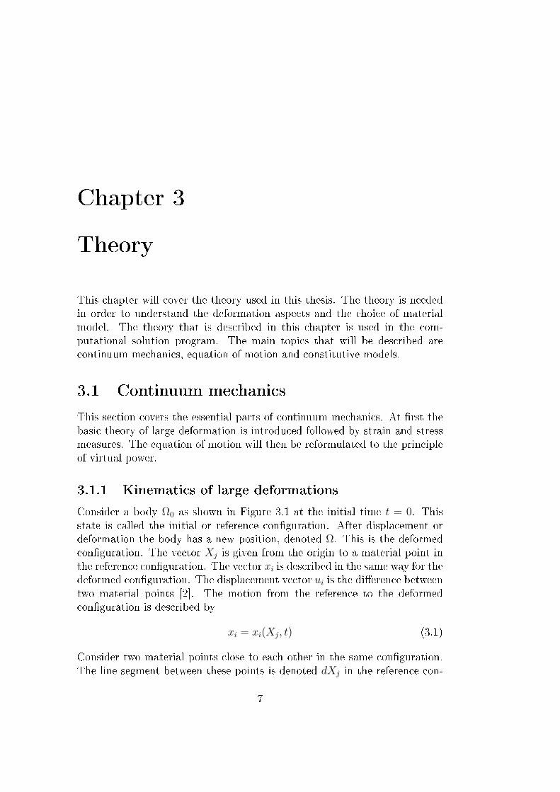
3.1.1 Kinematics of large deformationsConsider a body Ω0 as shown in Figure 3.1 at the initial time t = 0. Thisstate is called the initial or reference conguration. After displacement ordeformation the body has a new position, denoted Ω. This is the deformedconguration. The vector Xj is given from the origin to a material point inthe reference conguration. The vector xi is described in the same way for thedeformed conguration. The displacement vector ui is the dierence betweentwo material points [2]. The motion from the reference to the deformedconguration is described by

xi = xi(Xj, t) (3.1)

Consider two material points close to each other in the same conguration.The line segment between these points is denoted dXj in the reference con-

7

8 CHAPTER 3. THEORY

0

2 2

11

ΩΩ

x

x , X

x , X

X

u

Figure 3.1: Deformation from initial to deformed conguration [2].

guration respectively dxi in the deformed conguration. The linear relationbetween the line segments is uniquely dened by

dxi = FijdXj (3.2)

where Fij is the deformation gradient tensor which is dened as

Fij =∂xi

∂Xj

(3.3)

anddet(Fij) > 0 (3.4)

The polar decomposition theorem states that in continuum mechanics a de-formation gradient tensor Fij can be decomposed into a rotation matrix Rik

and a left stretch tensor Vkj [2].

Fij = RikVkj (3.5)

3.1.2 Strain measuresThe strain measure that will be considered in this thesis is the logarithmicstrain [3].

εkj = ln(Vkj) (3.6)This strain measure is appropriate for large deformation analysis since theelastic part is assumed to be small [3]. To dene the rate of deformation inthe system the velocity of a material particle is dened as

3.1. CONTINUUM MECHANICS 9

vi =∂xi

∂t(3.7)

The velocity dierence between two neighboring particles in the deformedconguration is

dvi =∂vi

∂xj

dxj = Lijdxj (3.8)

where

Lij =∂vi

∂xj

(3.9)

is the velocity gradient tensor in the deformed conguration. The velocitygradient tensor Lij can be decomposed into symmetric and antisymmetricparts according to

Lij = Dij + Wij (3.10)The rate of deformation tensor Dij is dened by

Dij =1

2

(∂vi

∂xj

+∂vj

∂xi

)(3.11)

and the spin tensor Wij as

Wij =1

2

(∂vi

∂xj

− ∂vj

∂xi

)(3.12)

3.1.3 Stress measuresThe Cauchy stress is based on the deformed conguration and thereby denesthe true stresses [2]. The Cauchy stress σij is dened as

ti = σijnj (3.13)

where ti is the traction vector and nj is the normal out of the surface in thedeformed conguration. Another type of stress measure to consider is thestresses in the reference conguration. These stresses are then calculated onthe undeformed surface and are called the nominal stresses, Pij, these aredened in a similar way as the Cauchy stresses. The nominal stresses areused in experimental measures.

t0i = Pijn0j (3.14)

10 CHAPTER 3. THEORY

0

Ω

F df

i

i j

df

n

0Ω

j

j

-1jkdf

n

Reference configuration Deformed configuration

Figure 3.2: Stress measures in current and deformed conguration [2].

3.2 Equation of motionThe equation of motion is formulated for an arbitrary part of the body inthe deformed conguration Ω according to Figure 3.2. The arbitrary bodyhas the volume V and a boundary surface S. The arbitrary body is aectedby the traction vector along the boundary surface and the inner body forcebi per unit mass in the body [4]. This is adopted in Newton's second law

∫

StidS +

∫

VρbidV =

∫

VρuidV (3.15)

where ρ is the mass density and ui is the acceleration. Further the divergencetheorem of Gauss states the following relation for an arbitrary vector qi

∫

VdivqidV =

∫

SqinidS (3.16)

The denition of the divergence of the vector qi,i is

divqi,i =∂qi

∂xi

(3.17)

This allows (3.15) to be expressed as∫

V(σij,j + ρbi − ρui)dV = 0 (3.18)

where σij,j is the divergence of the Cauchy stress. Since (3.18) holds forarbitrary regions V of the body, the equation of motion is obtained

σij,j + ρbi = ρui (3.19)The equation of motion is called the strong form. The principle of virtualpower, also called the weak formulation, is then obtained by multiplying the

3.2. EQUATION OF MOTION 11

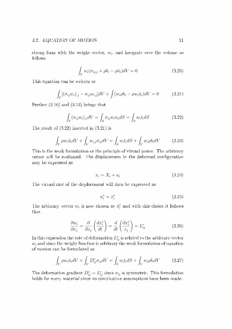
strong form with the weight vector, wi, and integrate over the volume asfollows

∫

Vwi(σij,j + ρbi − ρui)dV = 0 (3.20)

This equation can be written as∫

V[(σijwi),j − σijwi,j]dV +

∫(wiρbi − ρwiui)dV = 0 (3.21)

Further (3.16) and (3.13) brings that∫

V(σijwi),jdV =

∫

SσijwinjdS =

∫

SwitidS (3.22)

The result of (3.22) inserted in (3.21) is∫

VρwiuidV +

∫

Vwi,jσijdV =

∫

SwitidS +

∫

VwiρbidV (3.23)

This is the weak formulation or the principle of virtual power. The arbitraryvector will be evaluated. The displacement in the deformed congurationmay be expressed as

xi = Xi + ui (3.24)

The virtual rate of the displacement will then be expressed as

uvi = xv

i (3.25)

The arbitrary vector wi is now chosen as uvi and with this choice it follows

that

∂wi

∂xj

=∂

∂xj

(dxv

i

dt

)=

d

dt

(∂xv

i

xj

)= Lv

ij (3.26)

In this expression the rate of deformation Lvij is related to the arbitrary vector

wi and since the weight function is arbitrary the weak formulation of equationof motion can be formulated as

∫

VρwiuidV +

∫

VDv

ijσijdV =∫

SwitidS +

∫

VwiρbidV (3.27)

The deformation gradient Dvij = Lv

ij since σij is symmetric. This formulationholds for every material since no constitutive assumptions have been made.


3.3 Constitutive modelTo establish the constitutive model the stress rate, the yield stress criterionand the hardening model have to be determined. The formulation of Hill'sorthotropic yield criterion will be considered together with three dierenthardening models. The hardening models that are considered are isotropic,linear kinematic and combined hardening. These models can all be denedin ABAQUS.At rst small deformation is considered

εij = εeij + εp

ij (3.28)

where εeij is the elastic and εp

ij is the plastic strains. To establish a similarrelation in large deformation theory the deformation rate Dij is considered.The rate of deformation is decomposed into an elastic De

ij and a plastic Dpij

part as

Dij = Deij + Dp

ij (3.29)

An assumption is made that the stress rate is linearly related to the rate ofdeformation, this is the hypo elastic law.

Dσij

Dt= CijklD

ekl (3.30)

where Cijkl is a constitutive tensor and Dekl is elastic rate of the deformation

tensor from above. This assumption does not account for rigid body motionand therefore (3.30) is modied and called the Green-Naghdi rate

σGNij = CijklD

ekl − RlkRliσkj − σikRklRjl (3.31)

where Rik is the rotation tensor and Rlk is the rate of the rotation tensor [2].

3.3.1 Hill's orthotropic yield criterionThe yield criteria denes when a material will enter the plastic region. Foran isotropic material the von Mises yield criteria is often used. The yieldsurface has the shape of a circle in the deviatoric coordinate system accordingto Figure 3.3 since the stresses are equal in all directions. Materials thatbehave dierently when loaded in dierent directions are called anisotropic.If a material has three orthogonal symmetry planes the material is thencalled orthotropic. This means that the material is not fully anisotropic,

3.3. CONSTITUTIVE MODEL 13

examples of orthotropic materials are paper and wood. A way to introducean orthotropic yield surface is to use the Hill yield criterion

F (s2−s3)2+G(s2−s1)

2+H(s3−s1)2+2Ls2

23+2Ms212+2Ns2

13−1 = 0 (3.32)

The yield surface with the Hill criterion can be seen in Figure 3.3. Thiscriterion is applied to the packaging material that has dierent propertiesin the MD and CD. In (3.32) the 1-, 2- and 3-directions correspond to theMD, CD and ZD. The initial yielding in the Hill criterion is assumed to beaected only by deviatoric stresses, sij [5]. The deviatoric stress is denedas

sij = σij − 1

3σkkδij (3.33)

The criterion contains six independent material parameters. These can bedetermined by uniaxial stress tests and shear tests [6]. The material constantscan then be determined as

F = 12

[1

(σ1y0)2

+ 1(σ3

y0)2− 1

(σ2y0)2

]

G = 12

[1

(σ1y0)2

+ 1(σ2

y0)2− 1

(σ3y0)2

]

H = 12

[1

(σ3y0)2

+ 1(σ2

y0)2− 1

(σ1y0)2

]

L = 1

2(σ13y0)

2

M = 1

2(σ12y0)

2

N = 1

2(σ23y0)

2

(3.34)

where the σy0 is the yield stress. The Hill criterion can only be used whenthe yield surface is closed. This means that the following relation must besatised.

4

(σ1y0)

2(σ3y0)

2>

[1

(σ2y0)

2− 1

(σ3y0)

2+

1

(σ1y0)

2

]2

(3.35)

3.3.2 Hardening modelsHardening occurs when the stress in a material passes the yield stress andcan be determined by dierent hardening laws. The initial yield surface isdened as

F (σij) = 0 (3.36)


von Mises yield surface

Hill’s yield surface

32

1

σσ

σ

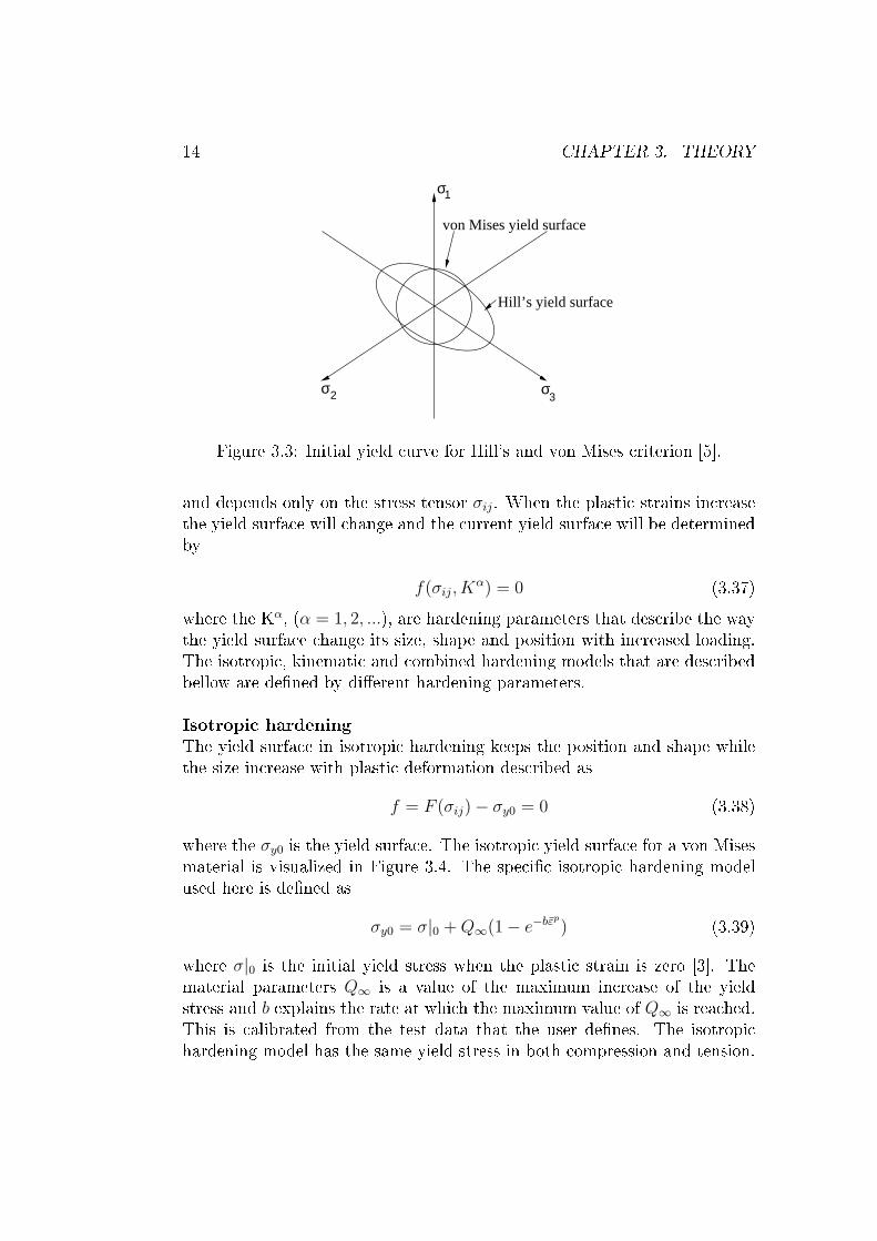
Figure 3.3: Initial yield curve for Hill's and von Mises criterion [5].

and depends only on the stress tensor σij. When the plastic strains increasethe yield surface will change and the current yield surface will be determinedby

f(σij, Kα) = 0 (3.37)

where the Kα, (α = 1, 2, ...), are hardening parameters that describe the waythe yield surface change its size, shape and position with increased loading.The isotropic, kinematic and combined hardening models that are describedbellow are dened by dierent hardening parameters.

Isotropic hardeningThe yield surface in isotropic hardening keeps the position and shape whilethe size increase with plastic deformation described as

f = F (σij)− σy0 = 0 (3.38)

where the σy0 is the yield surface. The isotropic yield surface for a von Misesmaterial is visualized in Figure 3.4. The specic isotropic hardening modelused here is dened as

σy0 = σ|0 + Q∞(1− e−bεp

) (3.39)

where σ|0 is the initial yield stress when the plastic strain is zero [3]. Thematerial parameters Q∞ is a value of the maximum increase of the yieldstress and b explains the rate at which the maximum value of Q∞ is reached.This is calibrated from the test data that the user denes. The isotropichardening model has the same yield stress in both compression and tension.

3.3. CONSTITUTIVE MODEL 15

3

2

1σ

σσ

Initial yield surface

Current yield surface

Figure 3.4: Isotropic yielding [5].

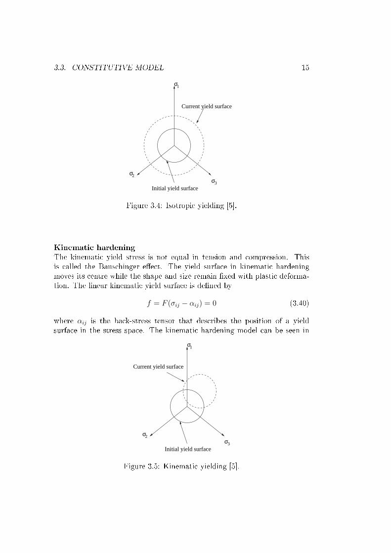
Kinematic hardeningThe kinematic yield stress is not equal in tension and compression. Thisis called the Bauschinger eect. The yield surface in kinematic hardeningmoves its centre while the shape and size remain xed with plastic deforma-tion. The linear kinematic yield surface is dened by

f = F (σij − αij) = 0 (3.40)

where αij is the back-stress tensor that describes the position of a yieldsurface in the stress space. The kinematic hardening model can be seen in


3

2

1σ

σσ


Figure 3.5: Kinematic yielding [5].


Figure 3.5 for a isotropic material. The evolution for the back stress tensoris based on Ziegler's hardening rule [3]

α = C1

σy0

(σ −α) ˙εp (3.41)

The components in (3.41) consists of the back-stress α, the back-stress rateα, the size of the yield surface σ0, the equivalent plastic strain ˙ε

p and thehardening parameter C. The initial yield surface is translated by the stressand back-stress tensors.

Combined hardeningThe combined hardening model is a mix of isotropic and kinematic hardeningdened by

f = F (σij − αij)− σy0 = 0 (3.42)The yield surface will therefore change size and position while the shapewill remain unchanged with plastic deformation, Figure 3.6. In ABAQUS


3

2

1σ

σσ


Figure 3.6: Combined yielding [5].

the combined hardening model is based on the non-linear kinematic and theisotropic hardening model, where the isotropic model is described by (3.39)and the kinematic [3] by

α = C1

σy0

(σ −α) ˙εp − γα ˙ε

p (3.43)

The nonlinearity is added in the kinematic hardening model (3.41) by theγα ˙ε

p term in (3.43). Here γ is a material parameter. The combined harden-ing model is preferably used when cyclic loading is involved.

Chapter 4

Numerical solution method

This chapter will explain the numerical solution method. The FE-formulationwill be dened as well as the computer program used in this thesis. The aimof the nite element method, FEM, is to solve problems where it is hardto determine an analytical solution. The FE-formulation is an method forsolving arbitrary dierential equations. The dierential equation to solve isthe equation of motion that is formulated as the principle of virtual power.This scalar equation will result in the FE-formulation. There are several dif-ferent programs on the market based on this theory. The simulation programused in this thesis needs to handle large deformation since the soft mater-ial will deform considerable during impact. Another important parameterfor the choice of simulation program is that nonlinear orthotropic materialproperties can be dened. It is also an advantage if the material can have or-thotropic behaviour in both the elastic and plastic range. This combinationof both elastic and plastic orthotropic behaviour is not very common todaybut is coming strongly. A simulation program that fulls these requirementsis ABAQUS. This simulation program is used to perform a large range ofanalyses. The main solvers are ABAQUS/Standard and ABAQUS/Explicit.These solvers will be explained further on in this chapter.

4.1 FE-formulationThe FE-formulation is built on the equation of motion (3.27) and will bewritten in matrix notation. At rst the approximation of displacement isdened bellow as

u = Na (4.1)

17

18 CHAPTER 4. NUMERICAL SOLUTION METHOD

where the interpolated displacement u is described by the shape function N.From this equation the acceleration vector is easy to derive and is presentedas

u = Na (4.2)The approximations above is used to compute the deformation rate as

Dv = Ba (4.3)where the b contains the derivative of the shape functions. From the Galerkinmethod [4] the weight function is determined as

w = Nc (4.4)Using (4.1)-(4.4) in (3.27) the following equation is obtained

cT(∫

VρNTNadV +

∫

VBT σdV −

∫

SNT tdS −

∫

VρNTbdV

)= 0 (4.5)

Now the FE-formulation starts to appear∫

VρNTNdV a +

∫

VBT σdV −

∫

SNT tdS −

∫

VρNTbdV = 0 (4.6)

where M, fint and fext are matrixes dened as

M =∫

VρNTNdV (4.7)

fint =∫

VBT σdV (4.8)

fext =∫

SNT tdS −

∫

VρNTbdV (4.9)

This results in the general FE-formulation

Ma = fext − fint (4.10)

4.2 Implicit vs explicit code formulationIn this section the implicit and explicit code formulation will be comparedto each other. ABAQUS/Standard can solve a wide range of various linearand nonlinear problems by using an implicit time integration scheme. This

4.3. EXPLICIT CALCULATION METHOD 19

means that the program iterate using the gradient of the next point to de-termine an acceptable solution. The slope of the function f(t) to the nexttime point t is illustrated in Figure 4.1. The implicit calculation methodoften iterate several times before an acceptable equilibrium has been found.The implicit calculation method is not suitable for dynamic impact prob-

0 1 2 3 4 50

1

2

3

4

5

6

7

8

t

f(t)

Figure 4.1: Implicit calculation method [7].

lems where contact is involved, in those cases ABAQUS/Explicit is recom-mended. This method is used for large deformation that occurs during ashort time. ABAQUS/Explicit applies the explicit time integration method,meaning that the last increment is used to anticipate the next step. In Fig-ure 4.2 the gradient of the start point is used to determine the function f(t)of the next time step t. The main dierence between ABAQUS/Standardand ABAQUS/Explicit is that the implicit method iterate while the ex-plicit method anticipate every step. The implicit method is always stablewhereas the explicit method is conditionally stable. This leads to that thedisk space and memory usage is much higher in ABAQUS/Standard analyses[3]. ABAQUS/Explicit is suitable for the application in this thesis consider-ing that the program is used for large deformation analysis with a short timeduration.

4.3 Explicit calculation methodThe explicit method is very ecient for problems with short load durationfor example in impact problems and explosions. ABAQUS/Explicit uses the


0 1 2 3 4 50

1

2

3

4

5

6

7

8

t

f(t)

Figure 4.2: Explicit calculation method [7].

explicit central-dierence integration rule to integrate the equation of motionfor a body [3]

Mu(i) = f(i)ext − f

(i)int (4.11)

The equation of motion is used to calculate the nodal acceleration u at everytime step using the diagonal mass matrix M, the applied load vector fext andthe internal force vector fint. The benet of the diagonal mass matrix is thatthe computational eort is reduced since the accelerations are solved directlyas

u(i) = M−1 · (f (i)ext − f

(i)int) (4.12)

and therefore requires no iterations. This calculation is performed at thebeginning of every increment. Further the acceleration is used to calculatethe velocity at the next time step

u(i+ 12) = u(i− 1

2) +

∆t(i+1) + ∆t(i)

2u(i) (4.13)

This requires that the initial velocity, u(i−12), is determined. When the ve-

locity is determined, the displacement can be calculated according to

u(i+1) = u(i) + ∆t(i+1)u(i+ 12) (4.14)

At the rst time step t=0 the velocity, u(0), and the acceleration, u(0), isdened by the user or is set to zero. To be able to use (4.13) and (4.14) theu(+ 1

2) and u(− 1

2) need to be calculated. This is done in the following equations

4.3. EXPLICIT CALCULATION METHOD 21

u(+ 12) = u(0) +

∆t(1)

2u(0) (4.15)

u(− 12) = u(0) − ∆t(1)

2u(0) (4.16)

The following steps in the explicit calculation are to determine the strainincrements in the elements and then the stresses. Finally the internal forcescan be computed. Now the next integration step can be performed. Thedisadvantage with an explicit method is that small errors are introducedwith time in the solution, which can make the solution unstable [5]. Toavoid this, the time increment has to be within a certain range. The timeincrement should be small enough that the acceleration within the incrementis constant. In ABAQUS/Explicit the stable time step with damping isobtained with

∆t ≤ 2

ωmax

(√

1 + ξ2 − ξ) (4.17)

where ξ is the fraction of critical damping in the highest mode [3] and ωmax

is the highest frequency in the system. A small amount of damping is intro-duced as bulk viscosity in ABAQUS/Explicit. This is done to improve themodelling of high-speed dynamic solutions because bulk viscosity introducesdamping associated with the volumetric straining [3]. The time step dependson if the FE-model contains one or several materials. When there is only onematerial the time increment is directly proportional to the size of the small-est element in the mesh. In uniform meshes with several materials the initialtime increment depends on the highest wave speed in the elements. The wavespeed cd is determined by Young's modulus E and the mass density ρ as.

cd =

√E

ρ(4.18)

Further ABAQUS/Explicit uses two strategies for supervising the time step,either calculating a new time increment or using a xed time step. Thewave speed cd and the smallest dimension Lmin in the mesh is used to get anapproximation of the stable time step.

∆t ≈ Lmin

cd

(4.19)

There are analyses that are nearly impossible to run since they require enor-mous amount of time to solve. One way to FE-simulate a time demanding


problem is to increase the mass of the part, so called mass scaling. The the-ory behind this solution are based on the equation (4.18) and (4.19). If thedensity ρ increases the wave speed cd will decrease. This leads to that thestability limit ∆t increases which will result in a shorter solution time. Themass scaling will have inuence on the inertia eects therefore the resultsneeds to be controlled to see that the inertia eects have not jeopardizedthe solution. Unfortunately it is not possible to mass scale the FE-model inthis thesis since this is not compatible with the EOS-formulation, used formodelling the water. The EOS-formulation will be discussed in chapter 6.2.

4.4 Energy balanceWhen using explicit integration methods it is necessary to control the energybalance. As already mentioned the explicit integration method can introducesmall errors if the time increment is too large. To verify if the solution isaccurate the energy values can be examined. The energy balance is denedin

EI + EV + EFD + EKE − EW = ETotal = constant (4.20)where EI is the internal energy, EV is the viscous energy dissipation, EFD

is the friction energy dissipation, EKE is the kinetic energy and EW is thework done by externally applied loads. The energies in (4.20) results in thetotal energy, ETotal. A good way to verify the solution is to investigate if thetotal energy is constant during the cause of the simulation. The total energyterm is constant since the energy can not disappear only be transformed. Innumerical methods the solution is not completely constant but should notvary by more than 1% [3]. The internal energy is the sum of the energiesdened by

EI = EE + EP + ECD − EA (4.21)where EE is the recoverable strain energy, EP is the energy dissipated throughinelastic processes such as plasticity, ECD energy dissipated through vis-coelasticity or creep and EA is the articial strain energy. The articialenergy is a measurement of energy stored in hourglass resistant and trans-verse shear in shell elements. If the articial energy is large the mesh shouldbe improved [3].

Chapter 5

Experimental test methods

To verify the simulations dierent experimental test methods are used toexamine if a correlation between a certain test method and the simulationsexist. The aim is to nd a parameter that can be evaluated in the simula-tion. Two dierent test methods are considered in this thesis, i.e. drop testand energy fracture test with dynamic pendulum. Both these methods arepracticed at Tetra Pak R&D but the dynamic pendulum will be applied fora dierent purpose than usually used.

5.1 Drop testThe drop test method is a very simple test method and corresponds well tothe reality. The disadvantage with this method is that the test only resultsin an intact or damaged package. There are no parameters that actually tellhow good the package resists an impact. The impact velocity of the package isa crucial parameter since large forces aect the package during a short tome.The impact velocity is dependent of the drop height. The impact positionof the package when hitting the ground is another parameter that can beinvestigated since all packages do not behave in the same way during impact.The position of the package before impact is dicult to see with the bareeye since the total impact in a drop test occurs in less than 200 ms. Furtherthe method is time demanding since several packages have to be dropped toget an indication of what height a package can handle. The parameters thatare tested are dierent package material and sealing types. Every time theseparameters change, a test series of 200 packages are dropped at 4-5 dierentheights. Package materials and sealings that manage a high drop height areevaluated further. The improvements are continued until the package reacha satisfactory height established by the development group.

23

24 CHAPTER 5. EXPERIMENTAL TEST METHODS

a) b)

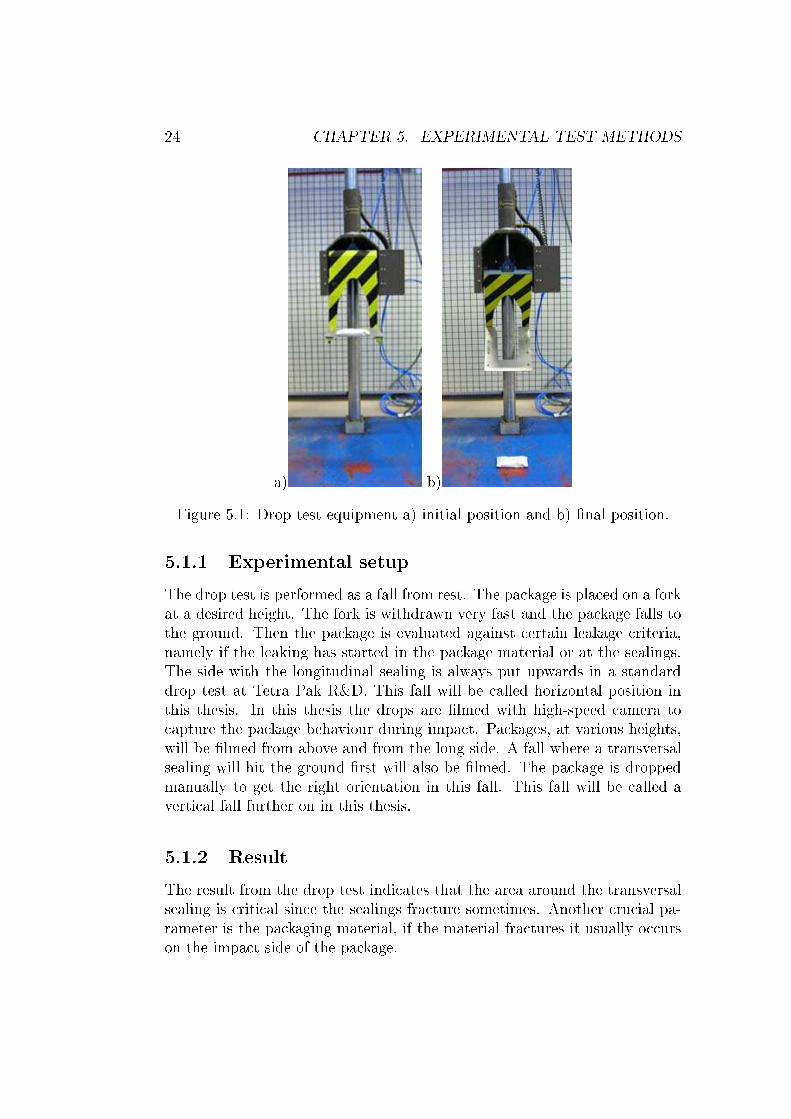
Figure 5.1: Drop test equipment a) initial position and b) nal position.

5.1.1 Experimental setupThe drop test is performed as a fall from rest. The package is placed on a forkat a desired height. The fork is withdrawn very fast and the package falls tothe ground. Then the package is evaluated against certain leakage criteria,namely if the leaking has started in the package material or at the sealings.The side with the longitudinal sealing is always put upwards in a standarddrop test at Tetra Pak R&D. This fall will be called horizontal position inthis thesis. In this thesis the drops are lmed with high-speed camera tocapture the package behaviour during impact. Packages, at various heights,will be lmed from above and from the long side. A fall where a transversalsealing will hit the ground rst will also be lmed. The package is droppedmanually to get the right orientation in this fall. This fall will be called avertical fall further on in this thesis.

5.1.2 ResultThe result from the drop test indicates that the area around the transversalsealing is critical since the sealings fracture sometimes. Another crucial pa-rameter is the packaging material, if the material fractures it usually occurson the impact side of the package.

5.2. DYNAMIC PENDULUM 25

Figure 5.2: A material crack in a package.

The high-speed lms made it possible to see how the package behaves duringimpact. The rst observation was that it is very dicult to receive an entirelyhorizontal impact position. The packages usually have an angular velocityor rotation that results in an impact that is dicult to analyze. This leadsto that the deformation behaviour in the high-speed lms depends on theimpact position. The vertical fall was a bit easier to lm since the packagehas its mass close to its centre of gravity. The result of the high-speed lmswill be used to evaluate the FE-simulated analysis further on in chapter 8.

5.2 Dynamic pendulumThe dynamic pendulum measures the energy absorption in a sample. Thistest method brings a measurement on the contrary from the drop test method.The dynamic pendulum test does not correspond to the reality as well as thedrop test method but it gives energy absorption levels that classies dier-ent materials. Another reason to evaluate this method is the fact that it isa dynamic method like the drop test. The dynamic pendulum test is per-formed on a sample of the transversal sealing in this thesis but it is usuallyperformed on a material sample. The transversal sealing is tested with thedynamic pendulum since it is near this area the damage is detected. Theexpectation for the dynamic pendulum test is to detect dierences in thematerial properties or the sealings and to obtain a parameter that can beused in the simulation.


Figure 5.3: Dynamic pendulum test equipment.

5.2.1 Experimental setupA pendulum that corresponds to the energy level of 0.5 J is positioned at axed height. Then a sample is positioned between two jaws, one xed andone movable. The pendulum is dropped and hits the moveable jaw. Thesample cracks into two pieces. The pendulum measures the energy that isrequired to crack the sample. The sealings are tested with the dynamic pen-

15

15

Sealing

5150

(mm)

Figure 5.4: Two sample geometries tested in the dynamic pendulum.

dulum since the drop test indicates that transversal sealing is a weakness inthe aseptic pouch. Three test sets were performed.

5.3. DISCUSSION 27

In the rst test set with the pendulum dierent parameters were tested toget an idea of which ones that made a dierence in the result. The testedparameters were dierent shapes of the samples and sealing types, accordingto Figure 5.4. A comparison was also performed between the top and bottomsealing. All the samples in the rst set were conditioned at 23C and 50%air humidity.In the second test set dierent material types were tested. The samples wereconditioned at 23C but at two dierent air humidities, 50% respectively80%.The last set of tests was performed at TFA-packages that actually had hugedierences in the drop test. This test was performed with the samples con-ditioned 23C and 50% air humidity since paperboard properties depends onthe humidity.

5.2.2 ResultIn the rst test setup there was no signicant dierence between the sealingtypes. No dierences were detected when the shape of the sample accordingto Figure 5.4 was considered in the evaluation process. The energy levels werea bit higher in the 15 mm samples than in the 5 mm samples but they werenot three times higher as expected. The test did not discover any actuallydierence in the energy absorption. After this set a decision was made toonly use the 5 mm samples since these were easier to prepare. In the secondtest setup where the humidity was changed no signicant dierences could bedetected. The result is showed in Figure 5.5. At last dierent TFA materialswere tested. The result shows that there are no signicant dierences betweenthese TFA package materials in the sealing. The energy absorption levels inthe TFA materials are about the same. Both materials absorb energy around0.20 J to 0.23 J. This can be compared to the energy levels in the sealingof the aseptic pouch that measures 0.16 J to 0.21 J at 50% air humidity.The total outcome from these results is that the dynamic pendulum did notdetect dierences in the sealings. Another result is that the pendulum couldbe too heavy for these types of packaging materials. The energy levels thatare measured with the 0.5 J pendulum are in the interval 0.16 J to 0.23 J.The pendulum has twice the energy that was needed to crack the samples.

5.3 DiscussionThe drop test method corresponds to the reality but it does not give anymeasures. The procedure of high-speed lming the impact during the drop


Figure 5.5: Energy absorbtion for the samples tested with various humidity.

test gives the opportunity to evaluate the simulation by comparing the be-haviour between the simulated and high-speed lmed package.The dynamic pendulum method has been tested on the transversal sealingsfor the aseptic pouch and TFA, since one of the critical areas are aroundthe sealing. The outcome of the tests shows that there are no signicantdierences between the sealings, not even when the samples were treated inhigher humidity.The result of the dynamic pendulum tests shows that the pendulum energyis twice of the energy absorption in the sample. It could be interesting to trya pendulum with a smaller energy level, perhaps around 0.20 J to be able tosee signicant dierences in the sealings.

Chapter 6

Material models

The material model that will be assigned in the FE-simulation will be estab-lished in this chapter. The packaging material has orthotropic properties inboth the elastic and plastic region. It is possible to assign both orthotropicelasticity and plasticity in ABAQUS 6.5. This has not been possible in earlierversions. The problem in this thesis contains large deformation, it is thereforeimportant that the material is properly dened in the plastic region. Theproperties of the water inside the package will be established by an equationof state, EOS.

6.1 Packaging material

The procedure to determine the material parameters for elastic and plasticbehaviour as well as the hardening models will here be described in detail.The packaging material is a laminate containing paperboard and polymers.The paperboard gives the laminate its orthotropic properties. In this thesisthe material parameters will be determined for the entire laminate and notfor each layer. The material data is obtained from tensile tests performed onthe packaging material in both MD and CD. As apparent from the tensilecurves in Figure 6.1 there are large dierences between the two directions.MD can handle higher strength while CD has better strain capability. TheZD properties are situated in the out of the plane direction and the strengthin this direction is much smaller than the other directions for paperboard.The packaging material that is used in this thesis is not available on themarket and therefore the measures are not shown in the tensile graphs inFigure 6.1 and Figure 6.3-6.5.

29

30 CHAPTER 6. MATERIAL MODELS

Nominal strain (%)

Nom

inal

str

ess

(MP

a)

MD

CD

Figure 6.1: Test data for the packaging material in machine and cross ma-chine direction.

6.1.1 Orthotropic elastic parametersA material enters the elastic region when it is loaded and no permanent strainoccurs. The material responds elastically until it reaches the yield stress,σyo. In the elastic region the Young's modulus E is determined. To obtaina proper material model with orthotropic properties the Young's modulusis determined for MD and CD. The orthotropic properties of the materialcan be dened in ABAQUS in several ways. One of them is to dene theelastic engineering constants for the material. The parameters are estab-lished by considering a tensile strain curve for the material. The orthotropicconstitutive relation between stress and strain is dened according to

ε = Cσ (6.1)

where ε, C and σ are dened as

ε11

ε22

ε33

γ12

γ13

γ23

=

1E11

−ν12

E13

−ν13

E330 0 0

−ν12

E11

1E22

−ν23

E330 0 0

−ν13

E11

−ν23

E22

1E33

0 0 0

0 0 0 1G12

0 0

0 0 0 0 1G13

0

0 0 0 0 0 1G23

σ11

σ22

σ33

σ12

σ13

σ23

(6.2)

where the 1-, 2- and 3 corresponds to MD, CD and ZD. The material en-gineering constants will be dened in this section. The Young's modulus is

6.1. PACKAGING MATERIAL 31

determined by calculating the slope of the tensile-strain curve in the elasticregion. The yield stress for MD is estimated from numerous test curves sincethe yield point is not distinguished in the graph. The Young's modulus isdecided in the same way for MD and CD. The relations that Baum [8] estab-lished are used to decide the Young's modulus in ZD and the shear modulus.These relations are established for paperboard properties and not for a lam-inate structure with polymers. The relations will here be used anyway sinceis assumed that the dominant properties in the laminate are received fromthe paperboard.

E3 =E1

200(6.3)

G12 = 0.39√

E1E2 (6.4)

G13 =E1

55(6.5)

G23 =E2

35(6.6)

6.1.2 Orthotropic plastic parametersPlasticity is one of the stages that many materials pass when loaded to frac-ture. From the yield point the material develops plastic strains. These strainswill remain even after unloading the material. If the load increases the plas-tic behaviour will continue until the material fractures. This behaviour isshown in Figure 6.2. The total strain is a combination of the elastic, εe, andplastic strain, εp.

εtij = εe

ij + εpij (6.7)

This formulation is only stated for small deformations but will here be usedto establish the plastic strains. In ABAQUS/Explicit the plastic behaviourof a material is described by assigning true stresses and true plastic strainsaccording to Cauchy theory. These are obtained from a stress-strain curveby converting the nominal measures. Nominal measures are calculated on anundeformed geometry while the true values depends on a deformed geometry.The true measures can be determined by using following relations

εtrue = ln(1 + εnom) (6.8)

σtrue = σnom(1 + εnom) (6.9)


σ

nomε

nom

total

ep

ε

εε

Figure 6.2: Tensile curve showing εe, εp and εtotal.

εp = εnom − εe = εnom − σtrue

E(6.10)

The orthotropic behaviour in the material is obtained by using Hill potential,see section 3.3.1.

6.1.3 Verifying hardening modelsThree hardening models in ABAQUS/Explicit, according to section 3.3.2, arecompared to decide which model that ts the experimental tensile test datathe best. The hardening models that will be examined are isotropic, linearkinematic and combined hardening model. A simple tensile test is simulatedto verify the hardening material models. When this is done the materialmodel can be implemented in the FE-simulation of a dropped package. Thetensile test is simulated similarly to the execution of the experimental test.In the FE-simulation the sample has the same geometry as the sample in thepractical tensile test. The sample has a rectangular geometry and containsonly one shell element. The material parameters are implemented as engi-neering constants for orthotropic elastic behaviour. To establish the plasticbehaviour Hill potential is used to dene the orthotropic properties withdierent hardening models. Plane stress is used since the problem is two-dimensional. The sample is xed at one short end in the loading direction

6.1. PACKAGING MATERIAL 33

and can not be rotated. The opposite end is displaced. The displacementis applied as a ramped function dened by an amplitude curve to preventchock loading in the sample. Two tests are performed since the materialpossesses orthotropic properties. In the rst test the displacement is appliedin the machine direction and in the other test in the cross machine direction.To verify that the material model behaves properly, the stress-strain curvesfrom the FE-simulation and the tensile test are compared. When simulatingin ABAQUS/Explicit the calculations are performed on deformed geome-try. The practical tensile test data are calculated per default on the nominalgeometry, see section 3.1.3. A FE-simulation was performed on both nominaland true geometry. The default setting in ABAQUS is to calculate on truegeometry. The dierences were small and therefore assumed to be negligible.The hardening is implemented from experimental data points according tosection 6.1.2. The data points should not be too many or have a large num-ber of decimals since this makes it harder to adjust a curve. The materialcurve is calculated to be adjusted to the material input data. To establishthe isotropic or combined material model several data points are requiredwhile the linear kinematic model only is dened by two points namely theinitial yield stress and the end point. The result of the simulated tensile testis shown in Figure 6.3-6.5.

Strain [%]

Str

ess

[MP

a]

Test Data Packaging materialABAQUS − Isotropic Hardening

MD

CD

Figure 6.3: Calibration of a material curve with isotropic hardening inABAQUS.


Strain [%]

Str

ess

[MP

a]

Test Data Packaging materialABAQUS − Kinematic Hardening

MD

CD

Figure 6.4: Calibration of a material curve with linear kinematic hardeningin ABAQUS.

Strain [%]

Str

ess

[MP

a]

Test Data Packaging materialABAQUS − Combined Hardening

MD

CD

Figure 6.5: Calibration of a material curve with combined hardening inABAQUS.

6.2. FLUID MATERIAL 35

6.1.4 ConclusionThe results from the verication of the hardening models shows that theisotropic hardening model corresponds best to the experimental test data.The combined model ts the test data well but is primarily used in cyclicloadings. The kinematic curve just approximates a linear hardening model.This suites problem exposed to large tensile stresses that transforms intocompression stresses. The isotropic hardening model is chosen since it suitsthe experimental tensile curves the best. The material model contains or-thotropic elasticity and isotropic hardening with Hill potential that will pro-vide orthotropic properties.

6.2 Fluid materialIn ABAQUS/Explicit an equation of state, EOS, can be used to model wateras a hydrodynamic material. This is done to give the solid elements its uidproperties. In this case a linear equation of state is used for the productin the package, that is as mentioned earlier the water. The linear EOS inABAQUS/Explicit describes a linear relation between volumetric strain andpressure. When dening EOS three parameters are required, c0, s and Γ0.The c0 parameter is the speed of sound in the uid and can be determinedby

c0 =

√K

ρ(6.11)

where K is the bulk modulus and ρ is the density. This only applies for a uidwith small compressibility [9]. The uid is assumed to be incompressible butis approximated to have small compressibility. The bulk modulus for wateris dened as K = 2.2 GPa and ρ = 1000 kg/m3 [10]. This results in aspeed of sound c0 = 1483 m/s. The material parameters s and Γ0 are bothnon-dimensional and are dened as zero on recommendation from ABAQUS-support since the uid is incompressible and non-viscous. A better way toFE-simulate the uid behaviour is to use computer software, like CFDesign,that is more suitable for uid solutions.


Chapter 7

FE-modelling in ABAQUS

The FE-simulations will be performed on an aseptic pouch lled with liq-uid to investigate whether it is possible to imitate the behaviour of a uidinside a soft beverage package during impact. This to analyse in whichway the packaging material is aected. The diculties with the analy-sis are to obtain a good geometry, correct material parameters and decidewhich parameters to evaluate. The FE-simulation will be performed in thecomputer program ABAQUS. The program contains several interacting soft-wares for instance ABAQUS/CAE and ABAQUS/Viewer. ABAQUS/CAEstands for Complete ABAQUS Environment and is a pre-processor. CAEis a graphical environment where models can be created or imported fromother CAD-systems. ABAQUS is divided into ten modules to facilitate theuse of the pre-processor. The modules are part, property, assembly, step, in-teraction, load, mesh, job, visualization and sketch according to Figure 7.1.ABAQUS/Viewer is a postprocessing tool that visualizes the result of ananalysis. This chapter describes the modelling procedure for a package that

Figure 7.1: A scheme of the modules in ABAQUS/CAE.

37

38 CHAPTER 7. FE-MODELLING IN ABAQUS

is exposed to a free fall. This drop test analysis contains three model parts;a package, a uid-geometry and a oor. The package with the uid inside isdropped on a rigid oor. To get an idea of how accurate the FE-simulationscorrespond to reality, high-speed lms of real drop tests are consulted. TheFE-simulations will later be veried in the visualization module against high-speed lms to see if the deformation behaviour is similar.

7.1 Modelling proceduresThe shape of the package that is studied in this thesis is very simple since thepackage only is a pouch lled with liquid. The modelling procedure is a bitmore dicult. One way to model the structure is to use several ellipses withdierent size as presented in Figure 7.2. The ellipses are used as a base whenlofting the uid volume. The lofting command calculates curves between theellipses and connects them together. One of these curves is illustrated inFigure 7.2. Every point on the ellipse has its own curve. Together the curvescan create a volume or an area.

Figure 7.2: Ellipses dening the package geometry.

At rst a solid part is created with the loft procedure that represents theuid in the FE-model. To verify the geometry of the uid, three parametersare examined

7.1. MODELLING PROCEDURES 39

Figure 7.3: Package created with loft.

• the circumferences of the ellipses are checked. All the ellipses shouldhave approximately the same circumference as the tube has during thelling process since it is this tube that is sealed into a package.

• the volume of the solid is veried to be 250 cm3 since the packagecontains 250 ml.

• the mass of the entire FE-model can be veried to 0.254 kg which isthe average weight of the package with water inside.

The geometry of the uid ends can be represented as straight lines since thetube is squeezed together. When performing the solid loft operation betweenthe ellipses and the straight lines a problem occurs. The solid loft operationdisapproves this kind of loft. The modelling procedure for the sealings willbe described further on in this chapter. The package is totally lled withuid which means that there are no cavities. This is a very important aspectto introduce into the simulation. In this thesis three dierent modellingtechniques were considered to create the uid and package interaction. Therst alternative is to create a package part from the outer surface of theuid part and then assign contact denition between the uid and the innersurface of the package. This is the most common technique when modellingcontact conditions. Unfortunately this technique is not proper for this FE-model since it was discovered at an early stage that the uid and the packagedid not interact very well since cavities occurred between the package and the


uid. This option will therefore not be further investigated in this thesis. Thesecond option is to improve the interaction between the uid and the packageto prevent the cavities that occurred in the previous method. This will bedone by merging the nodes from the two parts at the interacted surfaces.The merging nodes modelling technique will be described further in the nextsection. In the third method the package material was created based on theskin option that were found in the property module in ABAQUS/CAE. Theskin operation is actually performed on the solid mesh of the uid part andcreates a shell mesh representing the package. The skin modelling procedurewill also be discussed in detail in this chapter.

7.1.1 Model with merged nodesThis section will cover the modelling procedure with merged nodes. As men-tioned the package was created from the solid uid part. A copy is made ofthe solid part and then converted to the package shell part. This is an easytask to perform in the part-module. The choice of a shell part is based onthe fact that the packaging material is very thin and therefore well suitedfor shell elements. Further the parts are assembled, the uid is placed insidethe package. Since the uid and the package have the same size the uid iskept inside by the contact denition constraints with *ALL. This commandmakes sure that all parts are in contact with each other. The package andthe uid are meshed in a similar way but with dierent types of elements,shell respectively solid elements. An equal mesh can be accomplished if bothparts are partitioned and seeded in the same way. With the seed operationthe element mesh can be controlled by the element size or by number of ele-ments in a region. The purpose with the equal meshes is to enable mergingthe nodes. The nodes will be merged at the interacting surfaces betweenthe uid and the package. This procedure leads to that some elements sharenodes with each other but still keep their own element properties. In spiteof the fact that the meshes are divided in exactly the same way the nodeswill not match perfectly in the assembly. The reason is that when partitionthe parts the loft curve will be split and the entire shape changes in dierentways for the solid and shell parts. When splitting a loft curve the numberof interpolation points decrease and the curve gets a dierent appearance.There will be a dierence between the shell and the solid part since the loftprocedure calculates volumes and surfaces dierently. This causes problemsin the merging operation since the element nodes do not match perfectly witheach other for the dierent parts. In the merging procedure a tolerance ofthe largest distance that is allowed between the nodes is set. Only nodes inthe tolerance range will be merged. Observe that the tolerance range should

7.1. MODELLING PROCEDURES 41

not be larger than the smallest side of an element because then nodes withinone element will be merged. In this case the tolerance should not be largerthan 0.05 mm. Notice that when a merge node procedure is performed anentirely new part is created containing only an orphan mesh with its ele-ments. This means that material properties and boundary conditions mustbe assigned for the new mesh part. The materials and boundary conditionswill be described in further sections.

7.1.2 Model with skinIn this section the modelling procedure of the package with the skin operationin ABAQUS/CAE will be described. At rst the solid part is assigned itsuid properties and then the skin is positioned on the surface of the part.When creating a skin in the property-module, shell and material propertiesare assigned to the skin region. The surface of the shell elements coincidewith the upper surface of the uid elements. The part is then assembled withthe oor. The meshing procedure is performed by partitioning and seedingthe uid part. The uid part is assigned an explicit solid element type andthe skin is assigned an explicit shell element type. Then the uid part ismeshed, equal shell respectively solid elements and nodes positions appearin the part at the skin region. The skin is symbolizing the package and isinteracting with the uid inside since the nodes are shared between the solidand shell elements at the surface.

7.1.3 Choice of simulation modelIt is now time to evaluate the modelling procedure and choose the mostsuitable technique. When comparing the models it was found that the mod-elling procedure with skin has major benets compared to the merge nodemethod. The skin method is easy to use and fewer parts have to be created.The benet with one part is that it facilitates when changing parameters inthe package geometry since the changes only have to be performed in onepart. When performing a geometry change in the merge node FE-model,it has to be done in both the uid and package parts and then the entiremerge procedure must be performed all over again. The fact that the meshesmatch entirely which eliminates the cavities is another benet with the skinmodelling. In the FE-model with merged nodes cavities occurs during thesimulation since not all nodes at the surfaces are merged. As apparent theskin FE-model is to prefer, but it can be mentioned that it has its backsidestoo, especially when assigning the material orientation. When the materialorientation is assigned to the skin it can not be veried if the orientation is


properly applied before submitting the job. This is only possible to checkin ABAQUS/Viewer after submitting a job. The material orientation checkis easy to perform in a shell part, which is the case in the merging model.The possibility to visualize both uid and package in a cut plane position isan advantage for the merge node FE-model. The result of this evaluation isthat the skin FE-model is to prefer. The combination of easy modelling pro-cedure and good interaction behaviour between the uid and package makesthe skin modelling procedure to the preferred modelling strategy. In the nextsection the development of a nal FE-model with the transversal sealing isdescribed.

Figure 7.4: Longitudinal and transversal sealings in the package.

7.1.4 Sealings in the FE-modelThe nal FE-model will be built up with the skin operation and the twosealing types will be added according to 7.4. The transversal sealing willbe approximated to a rectangular shell element piece with double thicknessat each short side. As mentioned the solid loft operation does not approvewith letting a solid loft end with a straight line. The lofting will therefore beperformed as a shell loft and then converted to a solid part. This operationis performed to avoid the cavity. The lofting is performed from a straightline through the ellipses and ends in a straight line. A thing to think of whenlofting with an open loop is that the ellipses have to be created out of twoloops. This means that the ellipses should be divided into two pieces. To cre-ate the transversal sealing straight lines are created to make the transversalsealing 5 mm width. Finally a shell loft is performed between the uid end

7.2. ELEMENT TYPES 43

line and the new created line. The longitudinal sealing is created by applyingdouble package material thickness at the area where the longitudinal sealingis positioned. The skin modelling procedure continues as in section 7.1.2.

7.2 Element typesThe size of the element is important for the accuracy of the solution. A toorough mesh gives an inaccurate solution and a too ne mesh brings a moreaccurate solution but at the sacrice of a long solution time. The mesh den-sity in the current FE-model has the size of 1.1 mm and the time increment is1.5 · 10−7 s. It is now possible to determine the solution time of this analysisaccording to (4.19). The mesh density will be examined further on in thisthesis. To obtain a good mesh, dierent types of elements are used. The FE-model is mainly meshed with a structured mesh but close to the transversalsealings tetrahedron mesh are applied since the geometry is very complex inthis area. Shell elements are used to mesh the skin since the package is verythin. There are dierent types of shell elements in ABAQUS/Explicit, forthis case the S4R and S3R elements are used. The S4R element has 4 nodesand the S3R element has 3 nodes. These shell elements have conventionalstress and displacement properties and a large-strain formulation [3]. Theycan be used in three dimensional dynamic analyses and allows mechanicalloading. The shell elements also support reduced integration. This meansthat fewer Gauss points are used to calculate the stiness but the mass matrixand loads are integrated exactly. The problem with using fewer Gauss pointsis the rigid-body motions. These can occur for other displacements than thereal rigid-body motion. This depends on that fewer Gauss points can notdescribe the element in the same way as full integration. In solutions withfull integrations the stiness matrix is often too sti while the reduced inte-gration soften the stiness. If the rigid-body motion is controlled the reducedintegration may give a more accurate FE-model due to the stiness matrix[11]. Another advantage with reduced integration is that the running timesare shorter than with full integration. It should also be mentioned that fullintegration is not possible for S4R, S3R and C3D8R in ABAQUS/Explicit.When using reduced integrated elements it is necessary to be aware of thatthe hourglassing phenomena can occur.The uid part is modelled with solid elements. The uid properties of theelements are received by dening the density and EOS, according to chapter6.2. Appropriate solid elements for this analysis are the C3D8R respectivelyC3D4 element. These are three dimensional solid elements with 8 nodes.The element structure in the FE-model can be seen in Figure 7.5.


Figure 7.5: The element types in the FE-model.

The oor is modelled as an innitely sti part with innite mass. Thereforethe oor is only modelled with one element to reduce the computational ef-fort. The element type that is used in the oor is the R3D4-element. Thisis a three dimensional rigid element with four nodes, the third dimension isestablished by a thickness of the element.

7.3 Assigning packaging materialThe package contains both polymer and paperboard. The packaging materialhas higher strength properties in MD than in CD. This material behaviouris important to add in the FE-model. The material orientation is assigned inthe FE-model by creating a local coordinate system in the package and everyelement gets an appropriate material orientation. A shell element denitionhas 1- and 2-direction in the plane and the 3-direction is always the shellnormal. The material parameters were established in chapter 6.

7.4 Boundary conditionsTo solve the dynamic event, boundary conditions have to be introduced inthe FE-model. One of the most crucial conditions is the gravity but alsothe initial velocity and the impact point are important. Air resistance is ne-

7.5. FE-SIMULATIONS IN ABAQUS/EXPLICIT 45

glected in the analysis. To reduce the computational eort in the simulation,the package will always be dropped 1 mm above the oor. To be able toFE-simulate various heights the velocity of the package just before impactwill be calculated. This is based on the law of energy conservation that de-termines the connection between the drop height and the position above theoor.

mgh1 +mv2

1

2= mgh2 +

mv22

2(7.1)

v2 =√

2g(h1 − h2) (7.2)The velocity calculated with 7.2 will be the initial velocity in the FE-simulation.The velocity and gravity should be applied to both the package and the uidinside. The initial velocities and the corresponding kinetic energies thatwill be considered in these simulations are reported in table 7.1 In the FE-

Height [m] 0.3 0.8 1.3Velocity [m/s] 2.4 4.0 5.1Energy [J] 0.7 2.0 3.2

Table 7.1: Drop heights and corresponding initial velocities and energies.

simulation an impact point has to be established between the package andthe oor. The impact point is where the package will hit the ground initially.In this thesis the package will be dropped in two orientations as described inchapter 8. The friction between the package and the oor is assumed to benegligible since the package falls perpendicular to the oor.

7.5 FE-simulations in ABAQUS/ExplicitIn this section topics regarding solving analysis with the explicit method willbe discussed, for example step increments, double precision, CPU-time andimportant information that is stored in the les produced by ABAQUS whensubmitting a job.The total time in the FE-simulation should be adjusted to the problem toget an ecient simulation. This means that a long total time results in anunnecessary huge computational eort, long solution time and large resultles, especially the *.odb-le. These problems can be reduced in followingways. As already mentioned the total time should be minimized to reduce thesolution time. To reduce the solution time a higher number of CPU:s, CentralProcessing Unit, can be used for the explicit time integration method. This


is a very ecient method since the solution time can be decreased by 50 %using two CPU:s. Another way to decrease the size of the les is to optimizethe step increment. In the step increment the user decides the frequency thesolution stores data.It is recommended to use the option double precision when submitting a jobin ABAQUS/Explicit. Double precision means that more accurate numbersare used in the calculations, the oating point word lengths of 64 bits andthen the noise will be reduced in the simulation [3].When submitting a job in ABAQUS a number of les are produced and it is abit dicult to nd valuable information in them. Therefore a short overviewwill be made to bring forward the most utilized les. The most useful lesare the *.inp, *.dat and *.sta les. Interesting information that can be foundin the *.sta and *.dat les are summarized in table 7.2. The *.inp-le storesinformation from the CAE-module and is the le that is submitted to thesolver. It is a good idea to use the *.inp-le for data check. That means tocheck if all data is correct applied, for example in this case the initial velocityor the time step.

CPU-time *.sta number of elements *.dattime increment *.sta element size *.statotal mass *.sta warnings *.dat & *.stakinetic energy *.sta errors *.dat & *.sta

Table 7.2: Valuable information stored in the *.sta and *.dat les.

7.6 Summary of the modelling procedureNow it is time to summarize the modelling procedure to get a better overviewof the FE-model. The reader is asked to consult appendix A for a schematicoverview in ABAQUS/CAE. The scheme is a presentation of the various set-tings and parameters that are of importance. In this analysis SI units areused. At rst we have a uid part with a skin of shell elements at the surfacethat corresponds to the package geometry. The modelling procedure withskin was chosen since a better interaction was achieved between the packageand the uid. The package material model has orthotropic properties in boththe elastic and plastic range. The orthotropic properties are assigned accord-ing to the material orientation in the package. The uid is modelled withsolid elements and receives its uid properties by the equation of state, EOS.The components, longitudinal sealing and transversal sealings, are created in

7.6. SUMMARY OF THE MODELLING PROCEDURE 47

the FE-model with some simplications. The longitudinal sealing has doublethickness of packaging material symbolizing the overlap but no strip. Thetransversal sealings are approximated to double package material thicknessand triple in the region where the longitudinal and transversal sealing cross.Further the package is given an initial velocity and is dropped 1 mm abovethe oor to reduce the computational time. In this case it is also possibleto decrease the computational time by performing the calculations on twoCPU:s.


Chapter 8

Parameter variation and result

This chapter will cover the parameter variation of important settings in theFE-simulations and the results. The parameters that will be studied arevariable drop heights, the orientation of the package when it hits the oorand material parameters. The package will be dropped from two orientationsshown in Figure 8.1. The rst orientation is a drop where the longitudinalsealing is parallel to the oor and will be called the horizontal fall. This willbe the most common test position in the FE-simulations since this is thestandard position in the experimental drop test. The second choice is to letthe transversal sealing hit the oor rst and this will be called the verticalfall. All the FE-simulations will be performed at the reference height 0.8 mexcept those where various heights will be tested.When the package is drop tested it will hit the oor twice. The FE-simulationswill only cover the rst impact in order to reduce the solution time and thesize of the les. The rst impact is dened from the starting point until theentire package has left the oor. It is assumed that the critical stage for thepackage is during the rst impact. If the package fractures it will probablyhappen during the rst impact.The package has an ideal sealing in the FE-model that means that the sealingwill not burst. This depends on the modelling procedure where the transver-sal sealings are modelled as a straight lines and not with contact conditions.To model a crack mechanism a tensile failure condition could be applied butthis is only possible for isotropic materials in ABAQUS.

8.1 Horizontal fallThe packages are FE-simulated from various heights. This is done to inves-tigate if it is possible to detect dierences in the FE-simulation. The drop

49

50 CHAPTER 8. PARAMETER VARIATION AND RESULT

a) b)

Figure 8.1: Two main orientations of the package in the FE-simulations,a)horizontal orientation and b) vertical orientation.

tests are performed from 0.3 m, 0.8 m and 1.3 m. These heights are chosensince they represent three dierent scenarios. The package can handle a dropfrom 0.3 m and this height represent the intact package behaviour while the1.3 m drop corresponds to the damage package. A drop from 0.8 m is areasonable height from which the package should stay intact. One way tostudy if the FE-simulation behaves correct is to control the impulse of thedropped package. This is performed by calculating the momentum beforeand after the impact.

I =∫ t

0F (t)dt = m(v0 − v) (8.1)

When performing drop tests it was observed that the package hits the oorin various ways, since the package rotates during the fall. To capture thisphenomenon one package is rotated in the FE-simulation to hit the oor inan angled orientation. The orientation at impact will be estimated from ahigh-speed lm.

8.1.1 ResultThe deformation in the FE-simulation will mainly occur on the upside wherethe package dents as seen in Figure 8.2. Another deformation that is de-tected is a fold at the long sides of the package. When the package hits theoor the shock wave propagation can be seen on the underside. This is alsoreected in high stress concentration on the impact side, in both tension andcompression in the machine direction.

8.1. HORIZONTAL FALL 51

Figure 8.2: Deformation of a package dropped from 0.8 m at 4.5 ms.

Variable drop heightsThe purpose to FE-simulate the three various heights was to detect dier-ences. It is dicult to see dierent stress levels but it is possible to detectvariation in the concentration areas in the machine direction. These canbe seen in Figure 8.3. In the cross machine direction no dierences can bedistinguished and therefore will no picture of this behaviour be presented.Another interesting parameter to evaluate is the shear stresses since crackswith diagonal propagation have been detected in experimental drop tests.The shear stress in the plane direction is examined. For the shear stressconcentrations, no variations can be noticed between the heights. The shearstress for the drop from 0.8 m is presented in Figure 8.4. The amount of theshear stresses can not be investigated further in this thesis since this materialdata has not been determined for this material at Tetra Pak. The area withshear stresses corresponds with the regions where the cracks appear, compareFigure 8.5.One way to investigate when the impact occurs is to analyze the reactionforces in the oor. Various heights give dierent reaction forces in the oor.The reaction forces increases with the drop height as indicated in Figure 8.6.The graph also shows that the impact time last longer for low drop heights.Since the packages are dropped 1 mm above the oor with an initial velocitythe package with the highest speed will hit the oor rst. The reaction forces


a)

(Ave. Crit.: 75%)SNEG, (fraction = -1.0)S, Mises

-3.5e+07-2.5e+07-1.5e+07-5.0e+06+5.0e+06+1.5e+07+2.5e+07+3.5e+07+5.0e+07

b)

(Ave. Crit.: 75%)SNEG, (fraction = -1.0)S, S11

-4.9e+07-3.5e+07-2.3e+07-1.2e+07+1.0e+00+1.2e+07+2.3e+07+3.5e+07+5.0e+07

c)


-4.9e+07-3.5e+07-2.3e+07-1.2e+07+1.0e+00+1.2e+07+2.3e+07+3.5e+07+5.0e+07

Figure 8.3: Stress [Pa] in the machine direction -11 for the drop height a)0.3 m, b) 0.8 m and c) 1.3 m from a underside view.


a)


-1.1e+07-7.0e+06-4.7e+06-2.3e+06-2.5e-01+2.3e+06+4.7e+06+7.0e+06+1.1e+07

2 ms

b)


-1.1e+07-7.0e+06-4.7e+06-2.3e+06-2.5e-01+2.3e+06+4.7e+06+7.0e+06+1.1e+07

2.5 ms

c)


-1.1e+07-7.0e+06-4.7e+06-2.3e+06-2.5e-01+2.3e+06+4.7e+06+7.0e+06+1.1e+07

3 ms

Figure 8.4: Shear stress propagation in MD-CD for the drop height 0.8 mfrom a underside view.


a)

b)

Figure 8.5: a) Location of a material crack. b) Location of shear stress.


0 2 4 6 8 100

200

400

600

800

1000

1200

1400

Time [ms]

Rea

ctio

n fo

rce

[N]

Drop height 1.30 m

Drop height 0.8 m

Drop height 0.3

Figure 8.6: Reaction forces in the oor for various drop heights from hori-zontal falls.

a) 0 2 4 6 8 100

100

200

300

400

500

600

700

Time [ms]

Rea

ctio

n fo

rce

[N]

First impact

b) 150 155 160 165 1700

100

200

300

400

500

600

700

Time [ms]

Rea

ctio

n fo

rce

[N]

Second impact

Figure 8.7: Reaction forces in the oor from a 0.8 m drop during a) rstimpact and b) second impact.

in Figure 8.6 are not linear with the drop heights since the drop height is notlinear with the velocity. The areas under the graphs in Figure 8.6 representthe impulse that is dened in (8.1). The impulse is calculated by estimat-ing the velocities in the momentum before and after impact. The result isfound to be similar when comparing with the areas under the graphs. Theappearance of the graphs in Figure 8.6 depends on that few time intervalpoints have been saved in the FE-simulation. The amount of data pointsthat are saved highly aects the size of the solution le. This is the reasonthat only 40 data points are saved. The package's rst impact occurs after2.0 ms for the drop that symbolize the height 0.8 m. The second impactoccurs at 120 ms, presented in Figure 8.7, after that the package only hassmall movements.


Evaluation with high-speed lmsThe horizontal falls are compared with high-speed lms. It is dicult toobtain a complete horizontal impact in the drop test setup, section 5.1 sincethe fork tilt when it is withdrawn and may cause the rotation of the package.Another reason to this behaviour is that the centre of gravity is displacedin the package during the fall. The problem to obtain a complete horizontalfall leads to that the impact time dier between the high-speed lm and thesimulated animation. A FE-simulation with an estimated impact orientationwill be performed to simplify the evaluation procedure of the behaviour. Thisfall will be evaluated against a high-speed lm in Appendix B. It is dicultto achieve an estimated angle that corresponds with the angle in the high-speed lm. The problem is complicated by the rotation that often occurs inpractical drop test. This is why the deformation does not occur in the sameareas in the two cases. It is possible to see a tendency to similar behaviourbetween the FE-simulation and the high-speed lm.

8.2 Vertical fallThe vertical fall is tested in the FE-simulation to observe if it is possible tocapture the large deformations in the FE-simulation program, presented inchapter 3, that occur in this type of fall.

8.2.1 ResultWhen the package is dropped in a vertical orientation the water is gathered inthe lower part of the package. This leads to large deformation in this region.This behaviour corresponds well with the high-speed lm. The dierence isthat the package in the FE-simulation has larger deformations on the longsides. The comparison can be seen in Appendix B. The impact time inthe high-speed lm is estimated to 40 ms compared to the time in the FE-simulation that is 27 ms. It is dicult to establish the impact time in thehigh-speed lm since the dissolution is not as good as in the FE-simulationlms. This could be a reason that the impact time diers. Another sourceof errors could be that the air resistance is negligible in the FE-simulation.The reaction force for the vertical fall is much lower than for the horizontalas seen in Figure 8.8 but the impact last longer. This indicates on a moregentle impact for the vertical than the horizontal fall. The impulses in Figure8.8 are theoretically the same. When calculating the areas in the graphs the

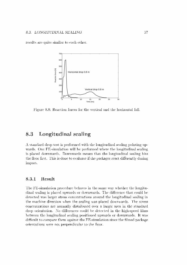
8.3. LONGITUDINAL SEALING 57

results are quite similar to each other.

0 5 10 15 20 25 300

100

200

300

400

500

600

700

Time [ms]

Rea

ctio

n fo

rce

[N]

Horizontal drop 0.8 m

Vertical drop 0.8 m

Figure 8.8: Reaction forces for the vertical and the horizontal fall.

8.3 Longitudinal sealingA standard drop test is performed with the longitudinal sealing pointing up-wards. One FE-simulation will be performed where the longitudinal sealingis placed downwards. Downwards means that the longitudinal sealing hitsthe oor rst. This is done to evaluate if the packages react dierently duringimpact.

8.3.1 Result

The FE-simulation procedure behaves in the same way whether the longitu-dinal sealing is placed upwards or downwards. The dierence that could bedetected was larger stress concentrations around the longitudinal sealing inthe machine direction when the sealing was placed downwards. The stressconcentrations are normally distributed over a larger area in the standarddrop orientation. No dierences could be detected in the high-speed lmsbetween the longitudinal sealing positioned upwards or downwards. It wasdicult to compare them against the FE-simulation since the lmed packageorientations were not perpendicular to the oor.


8.4 MaterialTo investigate the material dependency a thinner thickness was tested in theFE-simulation. The thickness was reduced by 20%.

8.4.1 ResultNo dierences were found when reducing the material thickness. The stressesand shear stresses were at the same level as before. The material propertiesout of the plane cannot be controlled since shell elements are used to createthe packaging material.

8.5 Mesh densityIn the explicit solution method the energy levels are controlled to establishthe correctness in the discretization of the FE-simulation model. If the en-ergy levels are acceptable a mesh density with fewer elements can be testedto achieve a shorter solution time. A mesh containing a larger amount of el-ements can also be tested to investigate if the deformation obtains a smotherappearance.

8.5.1 ResultAt rst a mesh containing less elements than the existing mesh was testedbut this mesh resulted in unstable energy levels according to Figure 8.9. Theinternal energy increased which is an indication for a bad mesh. Then amesh containing a larger amount of elements was tested. This resulted inthe same energy levels as the existing mesh in Figure 8.9. The mesh withlarger amount of elements had a 25% longer solution time than the existingmesh. Even though a smother appearance is obtained the cost of a longersolution time is considered to be to high.The interesting energies to investigate are plotted in Figure 8.9 and Figure8.10. The total energy is supposed to be constant in the solution and shouldnot vary more than 1% [3]. The total energy level in Figure 8.9 is constant.The initial level of the kinetic energy can be controlled in this FE-simulationsince this can be established from the energy of conservation law, Table 7.1.The kinetic energy will then decrease and the internal energy will increase.The internal energy consists of the strain energy and plastic dissipation.The strain energy will increase during the impact and will then turn backsince this only measures elastic deformation. The plastic dissipation will also

8.5. MESH DENSITY 59

a) 0 5 10 15 200

0.5

1

1.5

2

2.5

3

Time [ms]

Ene

rgy

[J]

total energykinetic energyinternal energy

b) 0 5 10 15 200

0.5

1

1.5

2

2.5

3

Time [ms]

Ene

rgy

[J]

total energykinetic energyinternal energy

Figure 8.9: a) Bad energy plot for the mesh containing less elements. b)Energy plot from the reference mesh.

a) 0 5 10 15 200

0.5

1

1.5

2

2.5

3

Time [ms]

Ene

rgy

[J]

plastic dissipationartificiall strain energystrain energy

b) 0 5 10 15 200

0.5

1

1.5

2

2.5

3

Time [ms]

Ene

rgy

[J]

plastic dissipationartificiall strain energystrain energy

Figure 8.10: a) Bad energy plot for the mesh containing less elements. b)Energy plot from the reference mesh.

increase during the impact but will then be stabilized since it measures apermanent deformation. The articial energy should be kept much smallerthan the internal energy. In this case the articial energy level is checked byenhanced hourglass control. Therefore the articial energy level is assumedto be corrected [3].


Chapter 9

Discussion

The FE-model with skin was selected among three dierent modelling tech-niques. This FE-model was chosen since it captures the interaction betweenthe packaging material and liquid the best. In the FE-simulations severalparameters have been studied. The package has been simulated in horizontaland vertical drops. The package in the FE-simulations behaved quite sim-ilar to the reality. This was concluded after analyzing the high-speed lmsand conducting practical tests. The phenomena that occur during an im-pact is that the upside of the package can deform while the impact side haveno ability to deform that leads to high stresses on this side. No dierenceswere observed in the deformation behaviour when the high-speed lms of thethree drop-heights were compared. Neither could a dierence be detected inthe deformation behaviour for the various heights in FE-simulation model.When comparing the high-speed lms with the FE-simulations similaritiesin the deformation behaviour were observed, even thou an estimated orien-tation is FE-simulated it is hard to fully capture the deformation behaviour.The package cannot burst since no fracture conditions are applied in theFE-model. In the evaluation process stress concentrations in the MD-CDplane was controlled in the packaging material. The package is modelledwith shell elements and therefore the stresses out of plane direction cannotbe examined. It is unfortunately not possible to evaluate the sealing areassince they are modelled as perfect sealings. The stress concentrations thatoccur around the transversal sealings cannot be evaluated since the cause ofthe stresses depends on geometry inaccuracy.In this thesis the dynamic pendulum was tested to investigate if a strengthparameter in the transversal sealing could be obtained. Unfortunately, nouseful result was obtained. An idea is to use a pendulum with a smallermass to investigate if a more precise result can be achieved. If this idea willbe tested the energy level in the pendulum should be a bit higher than the

61

62 CHAPTER 9. DISCUSSION

energy absorption in the samples. Hopefully this adjustment will result inmore accurate energy levels. If not so, the test method might not be suitableto measure the strength in the sealing.

9.1 ConclusionThe nal modelling technique is simple and easy to use. The benet withthis strategy is that it is easy to update the geometry in the FE-model. Thegeometry of the package can be controlled. For the aseptic pouch the cir-cumference, volume and mass can be veried against the real package. Itis also possibly to apply this technique on similar packages. The dicultieswere to capture the large deformation of a soft package and the interactionbetween the liquid and the package. The behaviour of the dropped packagesin the FE-simulations corresponds well compared to the high-speed lms.The FE-simulations show that high stress concentrations occur on the un-derside of the package. This seems to correspond well to the experimentaldrop tests since the material often fractures on this side. An observation isthat the cracks in the material often propagates diagonal from the corners.The shear stresses in MD-CD indicate on stress concentrations in the ex-posed areas. This result could be further investigated to establish if such acorrelation exists. Dierences in the stress concentration areas were detectedin the machine direction between the heights. This could be an interestingparameter to evaluate further since the aected areas could help to determineif a package can resist a drop.The reaction forces in the vertical fall are much smaller than for the hori-zontal. This is due to a larger amount of water that hits the oor at thesame time in the horizontal fall. In the vertical fall the package has a bettercapability to deform. The impact will also last for a longer time but the totalimpulse will be the same. The conclusion is that the vertical fall has a moregentle impact than the horizontal fall. The horizontal fall can therefore bedened as the most critical impact orientation. This behaviour correspondswell with the knowledge in project at Tetra Pak.The measurements obtained in the dynamic pendulum test did not indicateon any dierences between the tested samples. One conclusion that could bedrawn is that the pendulum probably is too heavy.Finally, the main purpose of this thesis is achieved since it has been shownthat it is possible to FE-simulate the dynamic event of a soft package droptest. Unfortunately no specic parameter that can predict the critical dropheight has been detected.

9.2. FURTHER WORK 63

9.2 Further WorkTo obtain better results several things can be improved in the FE-model.Specic areas that need to be improved are the sealings and the material de-scription. To be able to evaluate the transversal sealings the present sealingsneed to be replaced by a contact denition. It would therefore be desirableto have a measurement of the strength in the sealing to implement in thecontact denition.The material description can be improved by assigning the properties by thelamina command in ABAQUS. Each layer can be dened with the laminacommand. This will allow the material to have dierent bending propertiesin tension and compression. If it is desired to study the delamination be-tween the layers a model of the sealing should be created and implementedwith 3DM [12]. The 3DM-model considers both a continuum model and aninterface model where the interface model determines the delamination.To investigate if there is a connection between the cracks and the shearstresses experimental test can be used to nd this parameter. If the mate-rials show dierent strengths in the shear test this could explain why somematerials cracks easier.The drop test equipment can be improved by putting a high-speed scale onthe oor to measure the reaction forces during the impact. This would bringa measurement to evaluate in the drop test method. The reaction forcescould be compared with the ones calculated in the simulation.

64 CHAPTER 9. DISCUSSION

Bibliography

[1] Tetra Pak Marketing Services AB, Promotional Material,Lund, Sweden.

[2] T. Belytschko, Wing Kam Liu & Brian Moran Nonlinear Finite Ele-ments for Continua and Structures, Wiley 2001.

[3] ABAQUS documentation, Version 6.5

[4] O.C. Zienkiewicz & R.L. Taylor The Finite Element Method, Volume II.Butterworth Heinemann, Fith Edition, 2000.

[5] N. S Ottosen and M. Ristinmaa The Mechanics of Constitutive Mod-elling, Volume I-II, Division of Solid Mechanics, Lund University, 1999.

[6] A. Harrysson, M. Harrysson & M. Ristinmaa Current Models for Paperand Paperboard, Division of Solid Mechanics, Lund University, 2003.

[7] C. Führer & A. Schroll Numerical Analysis - An Introduction, 6th Edi-tion, Lund University, 2004.

[8] K.Persson Material model for paper - experimental and theoretical as-pects, Division of Structural Mechanics, Lund University, 1991.

[9] O.C. Zienkiewicz & R.L. Taylor The Finite Element Method, VolumeIII. Butterworth Heinemann, Fith Edition, 2000.

[10] http://hyperphysics.phy-astr.gsu.edu/hbase/sound/souspe2.html#c1,HyperPhysics Georgia State University

[11] N. S Ottosen & H. Petersson Introduction to the Finite Element MethodPrentice Hall Europe, 1992.

[12] O. Elison & L. Hansson Evaluating the 3DM model - an experimentaland nite element study, Division of Solid Mechanics, Lund University,2005.

65

66 BIBLIOGRAPHY

Appendix A

Package modelled in ABAQUS

A mind map was created to get an overview of the parameters used in the FE-simulation model. The map is based on the module setup in ABAQUS/Explicit.This mind map is created to increase the understanding for the modellingtechnique. The parameter variation that were discussed in chapter 8 aremarked in the mind map.

67

FE-mo

4. Step

Output variables

Field output

Select from list

reaction forcesdisplacement

stressstrain

velocityenergy

Space intervalnumber=200

History Output

Select from listenergy

Space intervalnumber=200

Dynamic explicit

Time period0.2 secNlgeom-on (default)

Bulk viscocitylinear - 0.06 (default)quadratic - 1.2 (default)

5. Interaction

Frictionm = 0

Contact*all with self

6. Load

Rigid floorGravity9.81 [m/s2]

Initial velocityvz = -3.96 [m/s]

7. Mesh

Hourglass controlenhanced control

Elements

SolidC3D4C3D8R

ShellS3RS4R

2D-rigid-floorR3D4

Seededge by number

Mesh controlsTetrahedralfree

Quadraticstructured

Nodesshared on surface

8. Jobdouble precision

CPU=2

9. Visualization

Reaction forces

Deformationshear stress

stressdisplacement

Energy

odel

1. Part

Floor 3D - discrete, rigid [m]

Fluid 3D - deformable, solid [m]

Package 3D - deformable, shell [m]

2. Property

Skin

Materials

WaterEOS

c0=1482 [m/s]s=0

0=0

Density 1000 [kg/m3]

TFA2

Density 895 [kg/m3]

Elasticity Engineering constants <=> Orthotropic

Plasticity Isotropic hardening potential (Híll)

Sections(shell homogenous)

Package t - thickness

LS 2*t

TS2*t3*t (with LS)width 5mm

Material orientation TFA2MDCDZD

3. Assembly

Package with fluid inside

Floor

Translated 0.001 mm

Horizontal fallVertical fall

Impact point

Sketch

(SI-units)

70 APPENDIX A. PACKAGE MODELLED IN ABAQUS

Appendix B

Comparing FE-simulations withhigh-speed lm

A comparison between the FE-simulated drops and the high-speed lms willbe shown in three picture sequence. These pictures are shown to give thereader an opportunity to observe the resemblance in the behaviour. The rstset of pictures describes the similarities in a horizontal fall from a side viewin Figure B.1. The high-speed lm captures the real behaviour the packageexperience during a fall from rest. The package in the simulation is placed ina similar angle to the oor to obtain a better agreement to the reality. Thenext picture series shows the same event but is lmed in an angle from abovein gure B.2. The last picture sequence presents a vertical drop position ofthe package in Figure B.3. All the drops in the pictures are performed from0.8 m.

71

72APPENDIX B. COMPARING FE-SIMULATIONSWITH HIGH-SPEED FILM

Figure B.1: Comparing horizontal falls in a side view.

73

Figure B.2: Comparing horizontal falls in a view from above.

74APPENDIX B. COMPARING FE-SIMULATIONSWITH HIGH-SPEED FILM

Figure B.3: Comparing vertical falls in a side view.

Appendix C

ABAQUS/Explicit input-le

75

76 APPENDIX C. ABAQUS/EXPLICIT INPUT-FILE

*Heading** Job name: DropSoftPackage Model name: nominell_model*Preprint, echo=NO, model=NO, history=NO, contact=NO**____________________________________________***** PART-FLOOR**____________________________________________***Part, name=Floor*Node

1, -0.5, -0.5, 0.2, 0.5, -0.5, 0.3, -0.5, 0.5, 0.4, 0.5, 0.5, 0.

*Element, type=R3D41, 1, 2, 4, 3*Node

5, 0., 0., 0.*Nset, nset=Floor-RefPt_, internal5,*Elset, elset=Floor1,*End Part**____________________________________________***** PART-FLUID**____________________________________________***Part, name=Fluid_content*Node

1, 0., 0., -0.07249999792, 0., 0., -0.0764999986...

62669, -0.0414670259, 0.00237717107, -0.06696761462670, -0.0413612947, 0.00255432609, -0.0659830123

***Element, type=C3D4

1, 28283, 5061, 28284, 282852, 28283, 5123, 28285, 28286...

8809, 7177, 7178, 690, 6898810, 7178, 1369, 41, 69062260, 101, 1521, 7633, 152862261, 1521, 1522, 7634, 7633

.

.

.74236, 10505, 10504, 2296, 229574237, 2304, 10505, 2295, 164***Element, type=C3D8R

8811, 4, 1058, 7179, 1376, 328, 6816, 28615, 71918812, 1058, 1057, 7180, 7179, 6816, 6817, 28616, 28615

.

.

.62258, 62609, 62607, 62567, 62568, 28281, 28282, 28260, 2825962259, 62607, 9683, 9680, 62567, 28282, 2069, 2068, 28260

77

*Element, type=S4R8271, 73, 1174, 6843, 11968272, 1174, 1175, 6844, 6843

.

.

.62669, -0.0414670259, 0.00237717107, -0.06696761462670, -0.0413612947, 0.00255432609, -0.0659830123

***Element, type=S3R74238, 6695, 6696, 102974239, 1049, 6694, 6697

.

.

.76808, 5095, 5112, 511476809, 355, 5107, 5114***Nset, nset=TS

3, 7 . . .*Nset, nset=LSTS

2, 3 . . .*Nset, nset=LS

59, 60 . . .*Nset, nset=Skin_Package

2, 3 . . .**** Region: (Water:Fluid_contetnt), (Controls:EC-1)** Section: Water*Solid Section, elset=fluid, controls=EC-1, material=Vatten1.,*Orientation, name=Ori-20., 0., 1., 1., 0., 0.3, 0.**** Region: (Skin_Package:Skin_Package), (Controls:EC-1), (Material Orientation:Package)*Elset, elset=Skin_Package, internal, generate63390, 74237, 1** Section: Skin_Package*Shell Section, elset=Skin_Package, orientation=Ori-1, controls=EC-1, material=Papper0.000122, 5*Orientation, name=Ori-10., 0., 1., 1., 0., 0.3, 0.**** Region: (TS:TS), (Controls:EC-1), (Material Orientation:TS)** Section: TS*Shell Section, elset=TS, orientation=Ori-1, controls=EC-1, material=Papper0.000244, 5*Orientation, name=Ori-10., 0., 1., 1., 0., 0.3, 0.**** Region: (LS_skin:LS_skin), (Controls:EC-1), (Material Orientation:LS)** Section: LS_skin*Shell Section, elset=_PickedSurf467, orientation=Ori-1, controls=EC-1, material=Papper0.000244, 5*Orientation, name=Ori-10., 0., 1., 1., 0., 0.3, 0.**** Region: (LSTS:LSTS), (Controls:EC-1), (Material Orientation:LSTS)** Section: LSTS*Shell Section, elset=LSTS, orientation=Ori-2, controls=EC-1, material=Papper0.000366, 5*End Part


**____________________________________________***** ASSEMBLY**____________________________________________*Assembly, name=Assembly***Instance, name=Fluid_content-1, part=Fluid_content3.49080188664863e-05, -0.0987023837026073, 0.0248711773551866*End Instance***Instance, name=Floor-1, part=Floor3.49080188526952e-05, -0.114702383702607, 0.02487117735518663.49080188526952e-05, -0.114702383702607, 0.0248711773551866,1.00003490801885, -0.114702383702607, 0.0248711773551866, 89.9999990194245*End Instance***End Assembly**____________________________________________***** ELEMENT CONTROLS**____________________________________________***Section Controls, name=EC-1, hourglass=ENHANCED1., 1., 1.**____________________________________________***** MATERIALS**____________________________________________***Material, name=Papper*Density895.,*Elastic, type=ENGINEERING CONSTANTS3.5e+09, 1.7e+09, 1.75e+07, 0.37, 0., 0., 9.43e+08, 6.4e+074.8e+07,

*Plastic1.7181e+07, 0.

2.4e+07, 0.0012.7e+07, 0.0023.3e+07, 0.0043.7e+07, 0.00634e+07, 0.008

4.3e+07, 0.014.7e+07, 0.0125e+07, 0.015

*Potential1., 0.5, 0.45, 0.4, 0.25, 0.15*Material, name=Vatten*Density1000.,*Eos, type=USUP1482.,0.,0.**____________________________________________***** INTERACTION PROPERTIES**____________________________________________***Surface Interaction, name=fric*Friction0.,**** Interaction: Int-1

79

*Contact, op=NEW*Contact Inclusions, ALL ELEMENT BASED*Contact property assignment, , fric**____________________________________________***** BOUNDARY CONDITIONS**____________________________________________**** Name: Rigid_floor Type: Symmetry/Antisymmetry/Encastre*Boundary_PickedSet109, ENCASTRE*****FIELDS**** Name: DropVel Type: Velocity*Initial Conditions, type=VELOCITYFluid_content-1.Fluid_contetnt, 1, 0.Fluid_content-1.Fluid_contetnt, 2, -3.96Fluid_content-1.Fluid_contetnt, 3, 0.** Name: Package_Vel Type: Velocity*Initial Conditions, type=VELOCITYFluid_content-1.Skin_Package, 1, 0.Fluid_content-1.Skin_Package, 2, -3.96Fluid_content-1.Skin_Package, 3, 0.** Name: TSVel Type: Velocity*Initial Conditions, type=VELOCITYFluid_content-1.TS, 1, 0.Fluid_content-1.TS, 2, -3.96Fluid_content-1.TS, 3, 0.** Name: LS_vel Type: Velocity*Initial Conditions, type=VELOCITYFluid_content-1.LS, 1, 0.Fluid_content-1.LS, 2, -3.96Fluid_content-1.LS, 3, 0.** Name: LSTS Type: Velocity*Initial Conditions, type=VELOCITYFluid_content-1.LSTS, 1, 0.Fluid_content-1.LSTS, 2, -3.96Fluid_content-1.LSTS, 3, 0.*****LOADS**** Name: gravity Type: Gravity*Dload, GRAV, 9.81, 0., -1., 0.****____________________________________________***** STEP**____________________________________________*Step, name=Step-1*Dynamic, Explicit, 0.02*Bulk Viscosity0.06, 1.2******* FIELD OUTPUT: F-Output-1***Output, field, number intervals=40*Node Output


A, PCAV, RF, U, V*Element Output, directions=YESELEDEN, ELEN, ENER, LE, PE, PEEQ, S*Contact OutputCSTRESS, PPRESS*****HISTORY OUTPUT: H-Output-1***Output, history, variable=PRESELECT, frequency=40*End Step

Documents

DROP TEST OF A SOFT BEVERAGE PACKAGE - Solid Mechanics