Embed Size (px)
Citation preview

3rd Student Conference onOperational Research
SCOR 2012, April 20–22, 2012, Nottingham, UK
Edited by
Stefan RavizzaPenny Holborn
OASIcs – Vo l . 22 – SCOR’12 www.dagstuh l .de/oas i c s

EditorsStefan Ravizza Penny HolbornSchool of Computer Science School of MathematicsUniversity of Nottingham Cardiff [email protected] [email protected]
ACM Classification 1998G.1.6 Optimization, G.2.1 Combinatorics, G.2.2 Graph Theory, G.2.3 Applications, I.2 Artificial Intelligence,I.6 Simulation and Modeling
ISBN 978-3-939897-39-2
Published online and open access bySchloss Dagstuhl – Leibniz-Zentrum für Informatik GmbH, Dagstuhl Publishing, Saarbrücken/Wadern,Germany. Online available at http://www.dagstuhl.de/dagpub/978-3-939897-39-2.
Publication dateJune, 2012
Bibliographic information published by the Deutsche NationalbibliothekThe Deutsche Nationalbibliothek lists this publication in the Deutsche Nationalbibliografie; detailedbibliographic data are available in the Internet at http://dnb.d-nb.de.
LicenseThis work is licensed under a Creative Commons Attribution-NonCommercial-NoDerivs (BY-NC-ND):http://creativecommons.org/licenses/by-nc-nd/3.0/legalcodeIn brief, this license authorizes each and everybody to share (to copy, distribute and transmit) the workunder the following conditions, without impairing or restricting the authors’ moral rights:
Attribution: The work must be attributed to its authors.No derivation: It is not allowed to alter or transform this work.Noncommercial: The work may not be used for commercial purposes.
The copyright is retained by the corresponding authors.
Digital Object Identifier: 10.4230/OASIcs.SCOR.2012.i
ISBN 978-3-939897-39-2 ISSN 2190-6807 http://www.dagstuhl.de/oasics

OASIcs – OpenAccess Series in Informatics
OASIcs aims at a suitable publication venue to publish peer-reviewed collections of papers emerging froma scientific event. OASIcs volumes are published according to the principle of Open Access, i.e., they areavailable online and free of charge.
Editorial Board
Daniel Cremers, TU Munich, GermanyBarbara Hammer, Uni Bielefeld, GermanyMarc Langheinrich, University of Lugano, SwitzerlandDorothea Wagner, KIT, Germany
ISSN 2190-6807
www.dagstuhl.de/oasics

Contents
PrefaceStefan Ravizza and Penny Holborn . . . . . . . . . . . . . . . . . . . . . . . . . . . . . . . . . . . . . . . . . . . . . . vii
Regular Papers
A Case Study on Optimizing Toll Enforcements on MotorwaysRalf Borndörfer, Guillaume Sagnol, and Elmar Swarat . . . . . . . . . . . . . . . . . . . . . . . . . . . 1
Revenue maximization through dynamic pricing under unknown market behaviourSergio Morales-Enciso and Jürgen Branke . . . . . . . . . . . . . . . . . . . . . . . . . . . . . . . . . . . . . . . 11
Empirical Bayes Methods for Discrete Event Simulation Performance MeasureEstimation
Shona Blair, Tim Bedford, and John Quigley . . . . . . . . . . . . . . . . . . . . . . . . . . . . . . . . . . . . 21
The Transition to an Energy Sufficient EconomyTimothy S. Mbasuen and Richard C. Darton . . . . . . . . . . . . . . . . . . . . . . . . . . . . . . . . . . . . . 31
Can online trading algorithms beat the market? An experimental evaluationJaveria Iqbal, Iftikhar Ahmad, and Günter Schmidt . . . . . . . . . . . . . . . . . . . . . . . . . . . . . . 43
An exact algorithm for the uncertain version of parallel machines schedulingproblem with the total completion time criterion
Marcin Siepak . . . . . . . . . . . . . . . . . . . . . . . . . . . . . . . . . . . . . . . . . . . . . . . . . . . . . . . . . . . . . . . . . . . 53
Product Form of the Inverse RevisitedPéter Tar and István Maros . . . . . . . . . . . . . . . . . . . . . . . . . . . . . . . . . . . . . . . . . . . . . . . . . . . . . 64
The design of transportation networks: a multi objective model combining equity,efficiency and efficacy
Maria Barbati . . . . . . . . . . . . . . . . . . . . . . . . . . . . . . . . . . . . . . . . . . . . . . . . . . . . . . . . . . . . . . . . . . . 75
Heuristics for the routing of trucks with double container loadsMichela Lai, Massimo Di Francesco, and Paola Zuddas . . . . . . . . . . . . . . . . . . . . . . . . . . 84
Optimization of electricity trading using linear programmingMinja R. Marinović, Dragana D. Makajić-Nikolić, Milan J. Stanojević, andLena S. Ðorđević . . . . . . . . . . . . . . . . . . . . . . . . . . . . . . . . . . . . . . . . . . . . . . . . . . . . . . . . . . . . . . . . 94
A Bilevel Mixed Integer Linear Programming Model for Valves Location in WaterDistribution Systems
Andrea Peano, Maddalena Nonato, Marco Gavanelli, Stefano Alvisi, andMarco Franchini . . . . . . . . . . . . . . . . . . . . . . . . . . . . . . . . . . . . . . . . . . . . . . . . . . . . . . . . . . . . . . . . . 103
3rd Student Conference on Operational Research (SCOR 2012).Editors: Stefan Ravizza and Penny Holborn
OpenAccess Series in InformaticsSchloss Dagstuhl – Leibniz-Zentrum für Informatik, Dagstuhl Publishing, Germany


Preface
We are delighted to present the proceedings of the 3rd Student Conference on OperationalResearch (SCOR 2012). The aim of SCOR is to provide PhD students in the early stagesof their OR careers with an excellent opportunity to meet other researchers with similarinterests and to present their work in a relaxed and friendly environment. In its third editionthe event was bigger and more international than ever before.
The conference took place from the 20–22 April 2012 at the University of Nottingham andwelcomed PhD students, mainly from European Universities, studying Operational Research,Management Science or a related field. Research areas included: Data Mining, DecisionSupport, Forecasting, Graphs and Networks, Healthcare, Heuristics and Metaheuristics,Inventory, Mathematical Programming, Multicriteria Decision Analysis, Neural Networksand Machine Learning, Optimisation, Reliability and Risk Assessment, Scheduling andTimetabling, Stochastic Modelling, Supply Chain Management, Simulation and SystemDynamics and Transport.
Some statistics from the event are as follows: there were 88 participants from 18 countrieswho provided 72 talks in up to 4 parallel streams over 3 days. There were 4 plenary talksgiven by Gavin Blackett (The OR Society), David Buxton (DSE Consulting Ltd.), TonyO’Connor (GORS) and Vincent Knight (Cardiff University) together with Louise Orpin (TheOR Society). These talks were extremely beneficial as they were aimed at giving delegates afeel for what could be next in their OR careers outside of academia.
In total there were 6 sponsors and we are extremely grateful for the sponsorship obtained,especially from The OR Society and from the ASAP research group at the University ofNottingham, which made this event possible.
As far as we are aware, this was the first time that a Smartphone app was used at an ORevent. This complemented the programme and book of abstracts. The main advantage ofthis app was that participants were able to personalise their own schedule for the event.
The review process was based on the presentation, quality and originality of the researchand there were at least two referees assigned to each paper. In total 21 submissions werereceived with 11 papers successfully accepted. These were from 6 different countries includingGermany, Hungary, Italy, Poland, Serbia and the United Kingdom demonstrating theinternational presence at the event.
We would like to give a special thanks to all authors who submitted a paper for review,to the Committee for their continued support and to all who contributed to the success ofSCOR 2012 and the proceedings.
Stefan RavizzaPenny Holborn
3rd Student Conference on Operational Research (SCOR 2012).Editors: Stefan Ravizza and Penny Holborn
OpenAccess Series in InformaticsSchloss Dagstuhl – Leibniz-Zentrum für Informatik, Dagstuhl Publishing, Germany


Organisation
Conference Committee
Stefan Ravizza, University of Nottingham, UK (Chairman)Penny Holborn, Cardiff University, UK (Vice-Chair)Michael Clark, University of Nottingham, UKEmily Cookson, Lancaster University, UKMagdalena Gajdosz, University of Strathclyde, UKPablo Gonzalez Brevis, University of Edinburgh, UKIzabela Komenda, Cardiff University, UKUrszula Neuman, University of Nottingham, UKMartin Takáč, University of Edinburgh, UKAlessia Violin, Université Libre de Bruxelles, Belgium
Additional Reviewer
Timo Kunz, Lancaster University, UK
Sponsors
The OR SocietyASAP research group, University of NottinghamProspect RecruitmentGower Optimal Algorithms Ltd.Tata SteelBanxia Software
3rd Student Conference on Operational Research (SCOR 2012).Editors: Stefan Ravizza and Penny Holborn
OpenAccess Series in InformaticsSchloss Dagstuhl – Leibniz-Zentrum für Informatik, Dagstuhl Publishing, Germany
A Case Study on Optimizing Toll Enforcements onMotorways∗
Ralf Borndörfer, Guillaume Sagnol, and Elmar Swarat
Zuse Institute Berlin Department OptimizationTakustr. 7, 14195 Berlin, Germany{borndoerfer,sagnol,swarat}@zib.de
AbstractIn this paper we present the problem of computing optimal tours of toll inspectors on Germanmotorways. This problem is a special type of vehicle routing problem and builds up an integratedmodel, consisting of a tour planning and a duty rostering part. The tours should guarantee anetwork-wide control whose intensity is proportional to given spatial and time dependent trafficdistributions. We model this using a space-time network and formulate the associated optimiz-ation problem by an integer program (IP). Since sequential approaches fail, we integrated theassignment of crews to the tours in our model. In this process all duties of a crew member mustfit in a feasible roster. It is modeled as a Multi-Commodity Flow Problem in a directed acyclicgraph, where specific paths correspond to feasible rosters for one month. We present computa-tional results in a case-study on a German subnetwork which documents the practicability of ourapproach.
1998 ACM Subject Classification G.1.6 Optimization, G.2.3 Applications
Keywords and phrases Vehicle Routing Problem, Duty Rostering, Integer Programming, Oper-ations Research
Digital Object Identifier 10.4230/OASIcs.SCOR.2012.1
1 Introduction
The Vehicle Routing Problem (VRP) is an extensively studied optimization problem with alot of variants and very different solution approaches, see [8, 4] for an overview. The core isalways to determine a set of tours to execute given tasks. In this paper we will present amodel to set up tours as well, but under some unusual settings and assumptions that lead toanother variant of vehicle routing problems.
We address the problem of computing tours for toll control inspectors on motorways.In 2005 Germany introduced a distance-based toll on motorways for commercial truckswith a weight of at least 12 tonnes. The enforcement of the toll is the responsibility of theGerman Federal Office for Goods Transport (BAG). It is implemented by a combination of anautomatic enforcement by stationary control gantries and by random tours of mobile controlteams. There are about 300 control teams distributed over the entire network. The teamsconsist mostly of two inspectors, but in some cases of only one. Each team can only controlhighway sections in its associated control area, close to the depot. Germany is subdividedinto 21 control areas. Our approach could also be applied to other countries and toll systemsif they use mobile control tours. Furthermore there must be central databases that provideon-demand information on drivers, if they have paid tolls or not.
∗ This work was funded by the German Federal Office for Goods Transport (BAG).
© Ralf Borndörfer, Guillaume Sagnol, and Elmar Swarat;licensed under Creative Commons License NC-ND
3rd Student Conference on Operational Research (SCOR 2012).Editors: Stefan Ravizza and Penny Holborn; pp. 1–10
OpenAccess Series in InformaticsSchloss Dagstuhl – Leibniz-Zentrum für Informatik, Dagstuhl Publishing, Germany
2 A Case Study on Optimizing Toll Enforcements on Motorways
Our challenge is to solve the VRP for the mobile teams. The tours should guarantee anetwork-wide control whose intensity is proportional to given spatial and time dependenttraffic distributions. Similar to classical vehicle routing problems we have a length restrictionfor all tours according to daily working time limitations. We model this problem using aspace-time network and formulate an associated optimization problem as an Integer Program.A typical problem instance is to compute a monthly plan for one control area of the Germannetwork.
The paper is structured as follows. In Section 2 the Toll Enforcement Problem (TEP) [2]is introduced and distinguished from classical vehicle routing approaches. In the followingsection the graph and IP model for the TEP is introduced and the integration of therostering part is presented. In Section 4 we explain our settings for the case study andthe computational experiments. Finally, in Section 5 the results are discussed and somedirections for future research are provided.
2 Optimal Toll Enforcement
In contrast to most of the Vehicle Routing problems, where a set of given demands or taskshas to be met, in the TEP this is different. Since the number of teams is fixed, the goal hereis to control as efficiently as possible with the available personnel. If we assign a profit valueto each section that could be covered by a tour, then our problem is related to a vehiclerouting problem with profits or a prize-collecting vehicle routing problem. In the case of onlyone vehicle this is known as the prize-collecting TSP (or TSP with profits). There are only afew applications for the case of several vehicles, see Feillet et al. [5] for a literature survey.A suitable approach to prize collecting in our setting is to set the profit to the number oftrucks that pass through a motorway section during a predefined time interval. This has theeffect to reward the controls on highly utilized sections. Furthermore, the profit values differduring different time intervals. For example, the section with the highest profit might not bethe same during the rush hour and during the night. Hence, not only the sections of a tourmust be determined, but also the starting time and the duration of a section control.
A second difference is with respect to driver assignments. Naturally vehicle routingproblems result in a set of tours. Drivers are assigned to the tours in a subsequent step. Thefeasibility of crew assignments is not part of the algorithms to solve the classical models.But in the toll control setting it is not possible to ignore the availability of crews. Thereare only a few drivers that can perform a planned tour since each tour must start and endat the home depot of its associated team. Thus, sequential approaches to plan the toursindependently of the crews will fail.
If we assign a crew to each tour, it must fit within a feasible crew roster, respecting alllegal rules, over a time horizon of several weeks. Minimum rest times, maximal amounts ofconsecutive working days, and labor time regulations must be satisfied. Hence, a personalizedduty roster planning must be used in our application. Therefore, we developed a novelintegrated approach, that leads to a new type of vehicle routing problems. To the bestknowledge of the authors there is no optimization approach to toll enforcement in theliterature yet. Related publications deal with problems such as tax evasion or ticket evasionin public transport; they mainly discuss the expected behavior of evaders or payers from atheoretical point of view, e.g. [1], or optimal levels of inspection, see [3].
R. Borndörfer, G. Sagnol, and E. Swarat 3
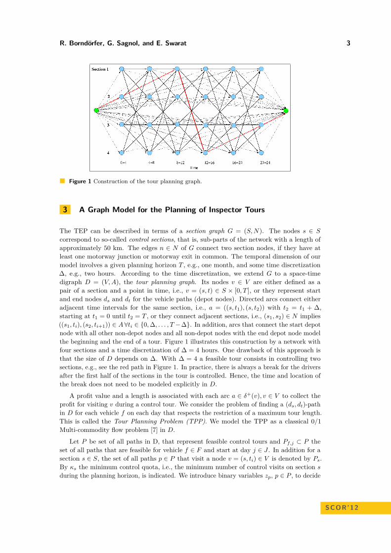
Figure 1 Construction of the tour planning graph.
3 A Graph Model for the Planning of Inspector Tours
The TEP can be described in terms of a section graph G = (S,N). The nodes s ∈ S
correspond to so-called control sections, that is, sub-parts of the network with a length ofapproximately 50 km. The edges n ∈ N of G connect two section nodes, if they have atleast one motorway junction or motorway exit in common. The temporal dimension of ourmodel involves a given planning horizon T , e.g., one month, and some time discretization∆, e.g., two hours. According to the time discretization, we extend G to a space-timedigraph D = (V,A), the tour planning graph. Its nodes v ∈ V are either defined as apair of a section and a point in time, i.e., v = (s, t) ∈ S × [0, T ], or they represent startand end nodes ds and dt for the vehicle paths (depot nodes). Directed arcs connect eitheradjacent time intervals for the same section, i.e., a = ((s, t1), (s, t2)) with t2 = t1 + ∆,starting at t1 = 0 until t2 = T , or they connect adjacent sections, i.e., (s1, s2) ∈ N implies((s1, ti), (s2, ti+1)) ∈ A ∀ti ∈ {0,∆, . . . , T −∆}. In addition, arcs that connect the start depotnode with all other non-depot nodes and all non-depot nodes with the end depot node modelthe beginning and the end of a tour. Figure 1 illustrates this construction by a network withfour sections and a time discretization of ∆ = 4 hours. One drawback of this approach isthat the size of D depends on ∆. With ∆ = 4 a feasible tour consists in controlling twosections, e.g., see the red path in Figure 1. In practice, there is always a break for the driversafter the first half of the sections in the tour is controlled. Hence, the time and location ofthe break does not need to be modeled explicitly in D.
A profit value and a length is associated with each arc a ∈ δ+(v), v ∈ V to collect theprofit for visiting v during a control tour. We consider the problem of finding a (ds, dt)-pathin D for each vehicle f on each day that respects the restriction of a maximum tour length.This is called the Tour Planning Problem (TPP). We model the TPP as a classical 0/1Multi-commodity flow problem [7] in D.
Let P be set of all paths in D, that represent feasible control tours and Pf,j ⊂ P theset of all paths that are feasible for vehicle f ∈ F and start at day j ∈ J . In addition for asection s ∈ S, the set of all paths p ∈ P that visit a node v = (s, ti) ∈ V is denoted by Ps.By κs the minimum control quota, i.e., the minimum number of control visits on section sduring the planning horizon, is indicated. We introduce binary variables zp, p ∈ P , to decide
SCOR’12
4 A Case Study on Optimizing Toll Enforcements on Motorways
that a tour is chosen or not. Then the following IP solves the TPP:
max∑p∈P
wpzp (1)
∑p∈Pf,j
zp ≤ 1, ∀(f, j) ∈ F × J (2)
∑p∈Ps
zp ≥ κs, ∀s ∈ S (3)
zp ∈ {0, 1}, ∀p ∈ P. (4)
In the objective function (1) the profit of the selected tours is maximized. Constraints (2)guarantee that each vehicle performs at most one tour per day. Constraints (3) requiresthat at least κs paths, that traverse section s, are chosen in a feasible solution. Finallyconstraints (4) demand the path variables being binary.
3.1 Integration of Duty Roster PlanningThe second task in the TEP is the planning of the rosters, called the Inspector RosteringProblem (IRP). There, the objective is to minimize the total costs. In contrast to many otherduty scheduling and rostering approaches the goal in this setting is not to minimize crewcosts. In the IRP the costs penalize some feasible but inappropriate sequences of duties, seeSection 4 for examples. This is more related to the criterion of driver friendliness.
We formulate the IRP again as a Multi-Commodity flow problem in a directed graphD = (V = (V ∪ {s, t}), A) with two artificial start and end nodes s, t. The nodes v ∈ Vrepresent duties as a pair of day and time interval. The arcs (u, v) ∈ A ⊆ V × V model afeasible sequence of two duties according to legal rules.
Let M be the set of all inspectors and bm the start value of the time account of m. Foreach month there is a regular working time for each inspector. This needs not to be metexactly, but there is a feasible interval for the nominal value of the working time account.Hence, by lm we denote the lower bound for the nominal value of inspector m and by um theupper bound, respectively. In addition, let tv be the duration of duty v ∈ V . The costs of adirect sequence of duties u and v ∈ V in a roster are indicated by cu,v. A variable xm
u,v foreach arc (u, v) and inspector m is introduced. According to that we propose the followinginteger programming formulation for the IRP:
min∑
m∈M
∑(u,v)∈A
cu,vxmu,v (5)
∑v
xms,v = 1, ∀m ∈M (6)∑
k
xmv,k −
∑u
xmu,v = 0, ∀v ∈ V ,m ∈M (7)
bm +∑u∈V
∑v
tuxmu,v ≤ um, ∀m ∈M (8)
bm +∑u∈V
∑v
tuxmu,v ≥ lm, ∀m ∈M (9)
xmu,v ∈ {0, 1}, ∀(u, v) ∈ A,m ∈M. (10)
R. Borndörfer, G. Sagnol, and E. Swarat 5
As already mentioned, in the objective function (5) the cost is minimized. By Constraints (6)we assure that exactly one arc per inspector with a non-zero flow value is leaving depots. The resulting path of all non-zero flow arcs for an inspector is called Inspector RosterPath. The flow conservation in the non-depot nodes is expressed by constraints (7). Theinequalities (8) and (9) enforce for each inspector that the planned roster does not exceedthe interval for the nominal value of the working time account. In the last constraint (10)the flow variables are restricted to be binary. In this model the use of arcs variables allows tohandle small and medium size instances, i.e., instances that have up to 160000 flow variablesin the rostering part.
Finally a formulation for the TEP is derived, by combining the TPP and the IRP byso-called coupling constraints. To this end, by Pf,v we define the set of all control pathsfeasible for vehicle f and duty v ∈ V . In addition, the parameter nf gives the numberof inspectors in vehicle f and m ∈ f denotes, that inspector m uses vehicle f in a fixedassignment. This leads to the following equation:∑
p∈Pf,u
nfzp −∑m∈f
∑v
xmu,v = 0 ∀f ∈ F, u ∈ V (11)
Each control path p belongs to a predefined time interval. Hence, by (11) it is guaranteedthat for each control path p in D all inspectors in the corresponding team have a feasibleroster path, where a duty in the time horizon of p is scheduled.
The objective function of the TEP is therefore a combination of collecting the profit (1)and minimizing the cost (5). In practice, we maximize a linear combination of these twoobjectives. A coefficient is used to set the proportion of the rostering costs in the integratedmodel. We have observed that for several instances, the solution which maximizes theprofit (1) contains no penalized duty sequence arcs (i.e., (5) is at its minimum). More detailsabout the rostering costs will be discussed in the next sections.
4 Case Study – Instances and Settings
We have implemented the above described model in an optimization tool, called TC-OPT.We tested TC-OPT on some real world instances from one control area with about 20inspectors. We used a set of standard (legal) rules, like minimum rest times, working timeregulations and some other constraints mentioned in the sections above. In addition, manuallygenerated reference plans from this control area are given. This allows a comparison of ournovel approach with plans that are representative for the current manual planning of thecontrol tours.
We selected six instances, three for August 2011 (aug1, aug2, aug3) and three for October2011 (oct1, oct2, oct3). Table 1 distinguishes the instances according to several criteria.The column “mincontrol for all sections” indicates whether we used the minimum controlquota constraint, see eq. (3), for all sections (case “yes”) or if some sections can be omittedduring control (case “no”). The fourth column gives information about so called “rotationpenalties” used in our model. This relates to the artificial costs we introduced in Section 3.1.A sequence of two duties d1 and d2 of an inspector from day t to day t+ 1 is called a rotation,if the starting-time of d2 is different from d1. If it starts later, e.g., from Mo 8-17 to Tu10-19, we call this a forward rotation. If the second duty begins earlier, e.g., Mo 8-17 to Tu6-15, it is a backward rotation.
SCOR’12
6 A Case Study on Optimizing Toll Enforcements on Motorways
Table 1 Overview on general settings for the test instances. All other parameter and data, e.g.,inspectors, teams, sections or holidays, are the same for all instances. If the data depends on the selectedmonth, it is the same in all instances belonging to the same month.
instance ∆ mincontrol for all sections rotation penalty traffic data fromaug1 4 yes moderate last monthaug2 2 yes moderate last monthaug3 4 no moderate last monthoct1 4 yes moderate last monthoct2 4 yes strong last monthoct3 4 yes moderate last year
It is legal to use rotations in a duty roster, if the minimum rest time between the end ofa duty and the beginning of the next is not less then 11h. Beside of that, is it an importantgoal to avoid or to minimize rotations in a roster. Because it is more employee-friendlyif subsequent duties start always on the same time and if changing to another start timeoccurs only after some days off. According to that we integrated rotation (penalty) factorsin our model which must be chosen in relation to the profit of the control tours. The value“strong” means that the penalty factors are higher then the profits of all tours while for“moderate” this holds only for a majority of the tours but not for all. In general the factorof the backward rotation should be higher, since this strongly infects the length of resttimes between duties. The last column indicates the period, from where we took the profitvalues in the objective function of the TPP (1). All data depending on the selected month,like holidays, fixed duties or working time accounts, are same in all of the three instancesbelonging to the same month. All other data, e.g. team assignments or the selection ofsections, are the same for all instances.
Another important aspect of the control planning is that a control may not start at anytime. There are given time intervals when the tours can take place. We call them workingtime windows. For our test setting we used six different time windows, two starting in themorning, one mid-day interval and three that start in the afternoon or in the evening. Amajor constraint in our model is that a certain duty mix is maintained. Therefore, for eachtime window there is a minimal and maximal contingent of all duties, e. g., the duties from6am to 3pm must be at least 20% of all duties and at most 50%. The main significance ofthese constraints is to define upper bounds on the number of late and night duties.
5 Case Study - Results and Discussion
We were able to solve all instances with a proven optimality. There is no optimality gapwith more than 10%. Hence, for all instances we received a feasible control plan. Beforethe solution behavior is dicussed in detail in Section 5.1 the quality of the optimized plansis analysed first. Comparing the manual and the optimized plan we see several benefits inusing TC-OPT. It is easier to handle the balance of the working hours, see eq. (8) and (9),especially in the case of different working hours in a team. The second is that we could complywith the duty mix constraints, which is more difficult in manual planning. Furthermore, itwas possible to prove the benefit in introducing the rotation factors. Comparing instanceoct2 to oct1 we were able to reduce the number of rotation when increasing the factor. Forsome instances, e.g., aug1, even a low factor suffices to avoid rotations between two scheduledduties.
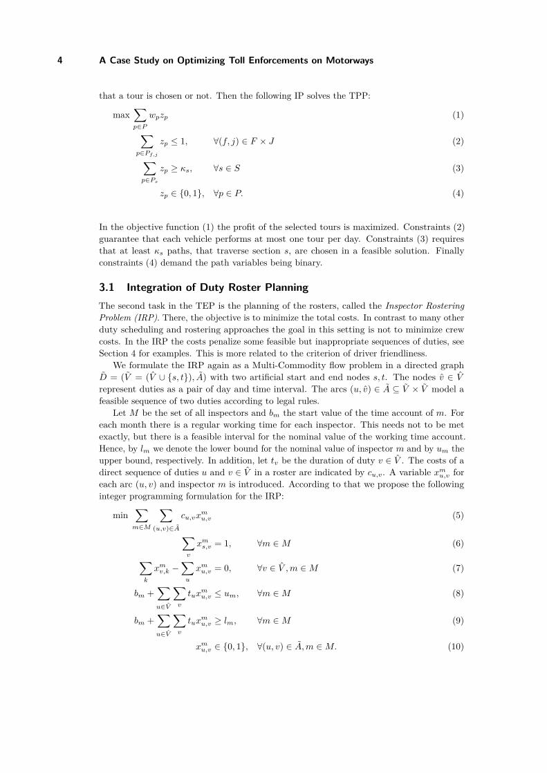
In Figure 2 the distribution of the controls on the 15 sections of the control area is shown.
R. Borndörfer, G. Sagnol, and E. Swarat 7
Figure 2 Control distribution over all sections in percent for instance aug1, the left blue columnsshow the reference plan, while the right columns in red represent the TC-OPT solution.
The main difference between the optimized and the reference plan is that the latter controlsa lot on sections five and six, while the optimized plan has a focus on sections seven andeight. The difference originates from the observation, that there is significantly more trafficon sections seven and eight than on five and six. The same holds for sections one and two,where TC-OPT controls the first section twice as much as the second one. So the objectivefunction clearly tends towards the sections with the most traffic. The sections with verylow traffic, like 12 or 15, were only controlled by the required minimum quota. We canconclude, that the control is mostly planned according to the traffic distribution. The useof minimum control quota constraints (3) achieves a better control coverage of the wholenetwork compared to the reference plans.
Choosing the time discretization to two hours, as in aug2, the control distribution alongthe sections is quite similar to the four-hour case. The only difference is a slightly higher partof the control on some low traffic sections. This originates from the possibility to control upto four sections during a tour in the two-hour case. As a result, one can control high trafficsections as well as low traffic sections in a common tour.
Another important aspect is the control distribution according to different days in a week.The main focus of the control is between Monday and Friday according to the fact that thereis much less traffic at the weekend. One reason for that is the Sunday truck ban on Germanmotorways that tolerates only small exceptions, e.g., for some urgent food transports.
Beside of the distribution over the weekdays it is interesting to study the distributionduring a day, i.e., a daily control pattern. It is important to mention that those values heavilydepend on the chosen duty mix constraints. Usually labour agreements restrict the numberof late and night shifts. Those regulations have a major impact on the mix constraints andthereby also on the daily control pattern. According to that, our optimization tool allowsthe planners to predefine the intervals for the duty mix constraints. This may have the sideeffect that the distribution can differ a lot between different areas.
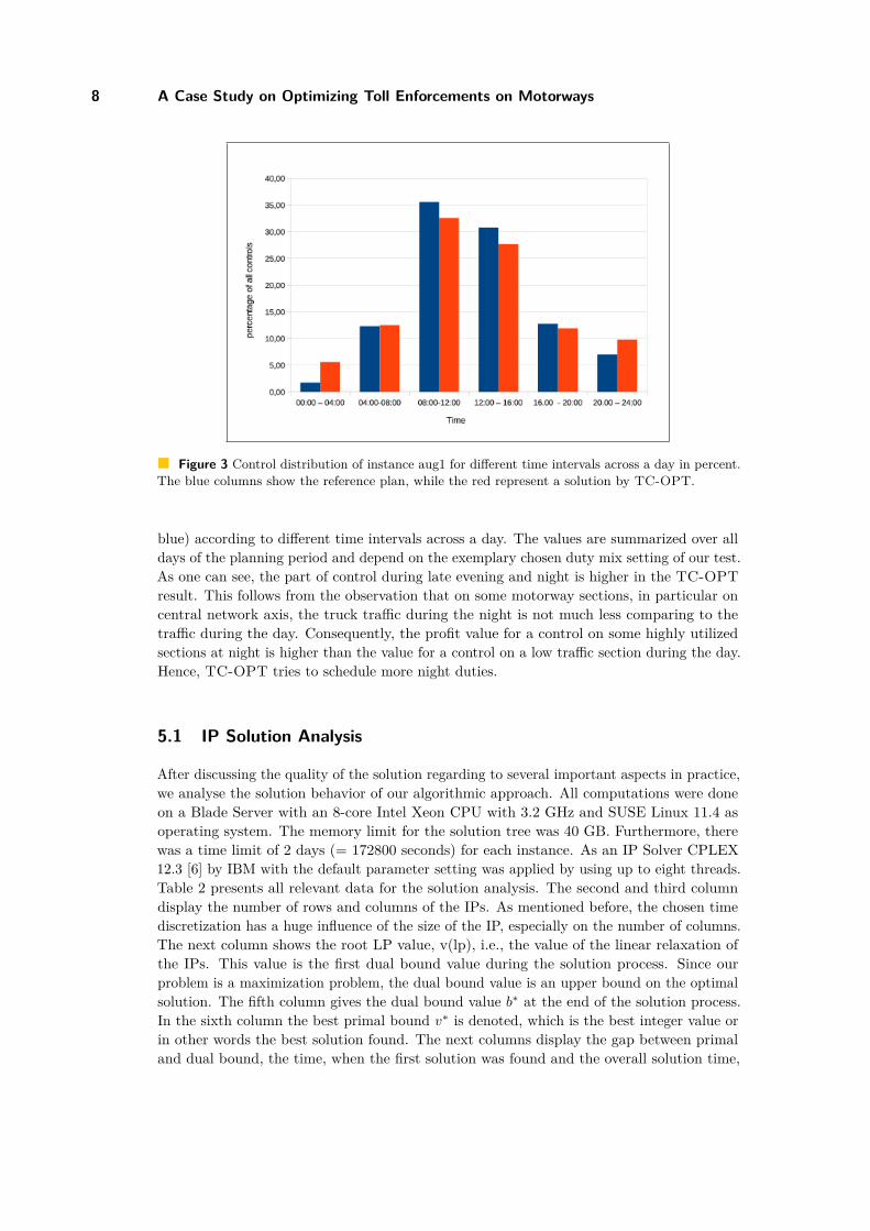
Figure 3 shows a comparison of the optimized plan (in red) and the reference plan (in
SCOR’12
8 A Case Study on Optimizing Toll Enforcements on Motorways
Figure 3 Control distribution of instance aug1 for different time intervals across a day in percent.The blue columns show the reference plan, while the red represent a solution by TC-OPT.
blue) according to different time intervals across a day. The values are summarized over alldays of the planning period and depend on the exemplary chosen duty mix setting of our test.As one can see, the part of control during late evening and night is higher in the TC-OPTresult. This follows from the observation that on some motorway sections, in particular oncentral network axis, the truck traffic during the night is not much less comparing to thetraffic during the day. Consequently, the profit value for a control on some highly utilizedsections at night is higher than the value for a control on a low traffic section during the day.Hence, TC-OPT tries to schedule more night duties.
5.1 IP Solution Analysis
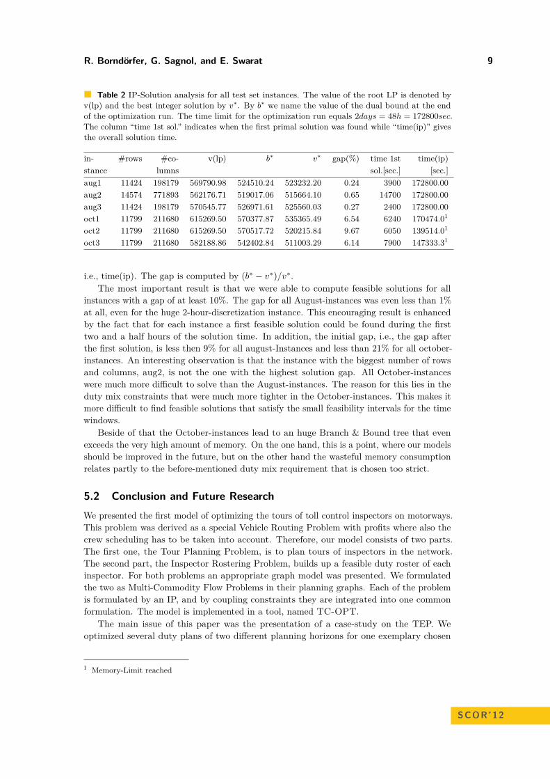
After discussing the quality of the solution regarding to several important aspects in practice,we analyse the solution behavior of our algorithmic approach. All computations were doneon a Blade Server with an 8-core Intel Xeon CPU with 3.2 GHz and SUSE Linux 11.4 asoperating system. The memory limit for the solution tree was 40 GB. Furthermore, therewas a time limit of 2 days (= 172800 seconds) for each instance. As an IP Solver CPLEX12.3 [6] by IBM with the default parameter setting was applied by using up to eight threads.Table 2 presents all relevant data for the solution analysis. The second and third columndisplay the number of rows and columns of the IPs. As mentioned before, the chosen timediscretization has a huge influence of the size of the IP, especially on the number of columns.The next column shows the root LP value, v(lp), i.e., the value of the linear relaxation ofthe IPs. This value is the first dual bound value during the solution process. Since ourproblem is a maximization problem, the dual bound value is an upper bound on the optimalsolution. The fifth column gives the dual bound value b∗ at the end of the solution process.In the sixth column the best primal bound v∗ is denoted, which is the best integer value orin other words the best solution found. The next columns display the gap between primaland dual bound, the time, when the first solution was found and the overall solution time,
R. Borndörfer, G. Sagnol, and E. Swarat 9
Table 2 IP-Solution analysis for all test set instances. The value of the root LP is denoted byv(lp) and the best integer solution by v∗. By b∗ we name the value of the dual bound at the endof the optimization run. The time limit for the optimization run equals 2days = 48h = 172800sec.The column “time 1st sol.” indicates when the first primal solution was found while “time(ip)” givesthe overall solution time.
in- #rows #co- v(lp) b∗ v∗ gap(%) time 1st time(ip)stance lumns sol.[sec.] [sec.]aug1 11424 198179 569790.98 524510.24 523232.20 0.24 3900 172800.00aug2 14574 771893 562176.71 519017.06 515664.10 0.65 14700 172800.00aug3 11424 198179 570545.77 526971.61 525560.03 0.27 2400 172800.00oct1 11799 211680 615269.50 570377.87 535365.49 6.54 6240 170474.01
oct2 11799 211680 615269.50 570517.72 520215.84 9.67 6050 139514.01
oct3 11799 211680 582188.86 542402.84 511003.29 6.14 7900 147333.31
i.e., time(ip). The gap is computed by (b∗ − v∗)/v∗.The most important result is that we were able to compute feasible solutions for all
instances with a gap of at least 10%. The gap for all August-instances was even less than 1%at all, even for the huge 2-hour-discretization instance. This encouraging result is enhancedby the fact that for each instance a first feasible solution could be found during the firsttwo and a half hours of the solution time. In addition, the initial gap, i.e., the gap afterthe first solution, is less then 9% for all august-Instances and less than 21% for all october-instances. An interesting observation is that the instance with the biggest number of rowsand columns, aug2, is not the one with the highest solution gap. All October-instanceswere much more difficult to solve than the August-instances. The reason for this lies in theduty mix constraints that were much more tighter in the October-instances. This makes itmore difficult to find feasible solutions that satisfy the small feasibility intervals for the timewindows.
Beside of that the October-instances lead to an huge Branch & Bound tree that evenexceeds the very high amount of memory. On the one hand, this is a point, where our modelsshould be improved in the future, but on the other hand the wasteful memory consumptionrelates partly to the before-mentioned duty mix requirement that is chosen too strict.
5.2 Conclusion and Future ResearchWe presented the first model of optimizing the tours of toll control inspectors on motorways.This problem was derived as a special Vehicle Routing Problem with profits where also thecrew scheduling has to be taken into account. Therefore, our model consists of two parts.The first one, the Tour Planning Problem, is to plan tours of inspectors in the network.The second part, the Inspector Rostering Problem, builds up a feasible duty roster of eachinspector. For both problems an appropriate graph model was presented. We formulatedthe two as Multi-Commodity Flow Problems in their planning graphs. Each of the problemis formulated by an IP, and by coupling constraints they are integrated into one commonformulation. The model is implemented in a tool, named TC-OPT.
The main issue of this paper was the presentation of a case-study on the TEP. Weoptimized several duty plans of two different planning horizons for one exemplary chosen
1 Memory-Limit reached
SCOR’12
10 A Case Study on Optimizing Toll Enforcements on Motorways
control area. A set of standard legal rules was integrated in our model. We were able tosolve all six instances with only a small optimality gap within two days. Furthermore, acomparison with a reference plan, that represents different aspects of traditional planningapproaches, showed that TC-OPT could support the planners. It was able to improve thequality of the optimized plan in many ways. Another important aspect of our case study isthe duration of the solution process. According to the usual planning horizon a duty planhas to be computed only once in a month. Hence, our time limit of two days is reasonablefrom a practical point of view. In urgent cases the time limit can be significantly reducedsince the first solution is found after a few hours in most cases.
Hence, it can be concluded that we are on the right way to get an optimization tool thatsatisfies all requirements of the toll control planning problem. An important aspect in ourfuture research is to be able to compute feasible plans for all control areas, with differentsettings in a reasonable time by moderate hardware requirements. We will test some impactsin our model to get smaller computation times, like problem-dependent reduction techniqueson the sizes of the planning graphs or variations on several parameters and strategies of theMIP solution process. Also additional rules, that are not legally defined, but very commonin practice, will be integrated in our model. A typical example is a fairer planning of lateand night shifts.
References1 M.G. Allingham and A. Sandmo. Income Tax Evasion: a Theoretical Analysis. Journal of
Public Economics, 1(3-4):323–338, 1972.2 R. Borndörfer, G. Sagnol, and E. Swarat. An IP Approach to Toll Enforcement Optimiz-
ation on German Motorways. Technical Report ZIB Report 11-42, Zuse Institute Berlin,Takustr. 7, 14195 Berlin, Germany, 2011.
3 C. Boyd, C. Martini, J. Rickard, and A. Russell. Fare Evasion and Non-Compliance: aSimple Model. Journal of Transport Economics and Policy, 23(2):189–197, 1989.
4 J.-F. Cordeau, G. Laporte, M. W.P. Savelsbergh, and D. Vigo. Vehicle Routing. InC. Barnhart and G. Laporte, editors, Handbooks in Operations Research and ManagementScience, Transportation, volume 14, chapter 6, pages 367–428. Elsevier, 2007.
5 D. Feillet, P. Dejax, and M. Gendreau. Traveling Salesman Problems with Profits. Trans-portation Science, 39(2):188–205, 2005.
6 IBM ILOG CPLEX, IBM Software Group. User-Manual CPLEX 12.3, 2011.7 R. M. Karp. On the Computational Complexity of Combinatorial Problems. Networks,
5(1):45–68, 1975.8 P. Toth and D. Vigo. The Vehicle Routing Problem. Society for Industrial and Applied
Mathematics, Philadelphia, USA, 2002.

Revenue maximization through dynamic pricingunder unknown market behaviourSergio Morales-Enciso1 and Jürgen Branke2
1 Centre for Complexity Science, The University of WarwickCoventry, CV4 7AL, [email protected]
2 Warwick Business School, The University of WarwickCoventry, CV4 7AL, [email protected]
AbstractWe consider the scenario of a multimodal memoryless market to sell one product, where a cus-tomer’s probability to actually buy the product depends on the price. We would like to set theprice for each customer in a way that maximizes our overall revenue. In this case, an explorationvs. exploitation problem arises. If we explore customer responses to different prices, we get apretty good idea of what customers are willing to pay. On the other hand, this comes at the costof losing a customer (when we set the price too high) or selling the product too cheap (when weset the price too low). The goal is to infer the true underlying probability curve as a functionof the price (market behaviour) while maximizing the revenue at the same time. This paperfocuses on learning the underlying market characteristics with as few data samples as possibleby exploiting the knowledge gained from both exploring potentially profitable areas with highuncertainty and optimizing the trade-off between knowledge gained and revenue exploitation.The response variable being binary by nature, classification methods such as logistic regressionand Gaussian processes are explored. Two new policies adapted to non parametric inferencemodels are presented, one based on the efficient global optimization (EGO) algorithm and thesecond based on a dynamic programming approach. Series of simulations of the evolution of theproposed model are finally presented to summarize the achieved performance of the policies.
1998 ACM Subject Classification I.2.6 Learning
Keywords and phrases Dynamic pricing, revenue management, EGO, Gaussian processes forclassification
Digital Object Identifier 10.4230/OASIcs.SCOR.2012.11
1 Introduction and literature review
Dynamic pricing is a strategy which aims to offer different prices for the exact same productto different customers. In general, this strategy is followed in order to maximize a firm’srevenue by understanding how the market reacts to different prices.
Depending on the nature of the service or product offered, there are different possiblescenarios. When designing a dynamic pricing policy, the distinction on whether finite orinfinite inventories and time horizons are being considered is important. Another possibledistinction is the nature of the market in terms of buying recurrence and the existence of aprecedent reference price because recurrent customers for an already established product havebeen shown to develop a peak-end memory effect which influences their behaviour towardsprice changes [13]. In this paper, we consider the memoryless scenario with an infinite timehorizon and infinite inventory. This is commonly the case when a new non seasonal product
© Sergio Morales-Enciso and Jürgen Branke;licensed under Creative Commons License NC-ND
3rd Student Conference on Operational Research (SCOR 2012).Editors: Stefan Ravizza and Penny Holborn; pp. 11–20
OpenAccess Series in InformaticsSchloss Dagstuhl – Leibniz-Zentrum für Informatik, Dagstuhl Publishing, Germany
12 Revenue maximization through dynamic pricing under unknown market behaviour
is introduced to the market and both the expected life cycle of the product and the availableinventory are sufficiently large.
Dynamic pricing strategies have been long studied in the context of physical distributionchannels where advertised prices are targeted to the whole market and every price changecarries a cost. Examples of this can be tracked back to revenue management research inthe airline industry started in the 70s [10], or to [7] where optimal policies are studied forseasonal products with finite inventories sold through physical distribution channels. Thesestudies try to understand the behaviour of the demand in terms of the arrival rates, whichis affected after a period of time when prices are changed for a given epoch. Since all themarket has access to the same information (advertised price), a change in the arrival rate ofcustomers who actually buy is expected.
In the current market conditions, the internet offers a perfect scenario for dynamic pricing,since prices can be changed individually for each customer without incurring any cost. In fact,this is already a common practice among internet retailers as is shown by the controversialexample of Amazon.com, which in September of 2000 ran a randomized pricing test acrossdifferent customers [17], along with many other examples which are described in [9]. Manyrecent studies considering the internet as a distribution channel and accounting for morefrequent price changes have been developed. An interesting characteristic of the recentstudies is that they all consider the relation between the advertised price and the arrivalrate of the buying customers as a descriptive measure of the market behaviour, like whendealing with physical distribution channels. Furthermore, most of the reviewed papers use aparametric regression model when inferring the demand curve, imposing a functional form tothe unknown market behaviour (e.g. [3], [1], and [4]). Some of the studies justify the choiceof a parametric model (like [6]), and only a few make use of non parametric models [2].
In order to take full advantage of the virtual markets, and keeping in mind that the firmaims to maximize the accumulated revenue and not to control the market behaviour, differentprices can be quoted to each customer without disclosing the quoted price to the rest of themarket. However, the fact that the information is not available to everyone removes therelationships between the quoted prices and the rate of arriving customers. For instance,reducing the price of a product will not necessarily increase the arrival rate of customersunless it is widely advertised, which is exactly what would be avoided in real cases if themarket price sensitivity is to be studied. Because of this, we propose to estimate the overallmarket price sensitivity through the estimation of the probability of buying a product givena quoted price (see section 2), and we assume constant arrival rates, removing the needof a time index. The traditional approach to this problem and our proposed approach areequivalent in the sense that the arrival rate of customers with probability 1 of buying –asmodelled in the former– and the probability of customers (buying and not buying) arrivingat a constant rate –as proposed it the latter– are interchangeable. The difference mainlyrelies in the number of samples needed to understand the market behaviour and the way ofperforming the experiment, i.e. quoting undisclosed prices directly to the customer.
The goal of this paper is to provide insight on which is the best pricing policy to followin order to maximize the accumulated revenue of a firm having to determine the price ofa product in an unknown market under the described framework. We propose 2 policies(EGO and one step lookahead in revenue) and compare their performance with another 2policies known in literature (random exploration and greedy) as well as with the optimalsolution as a benchmark, since in a realistic scenario it would be unknown. EGO (Effectiveglobal optimization) policy is based on the methodology outlined in [8] and takes samples atthe maximum expected improvement point. The one step lookahead policy is based on a
S. Morales-Enciso and J. Branke 13
dynamic programming approach and maximizes the overall revenue of the 2 next samples,which implicitly takes into account the information gained during the first sample, but doesnot include an explicit term to quantify information acquisition as opposed to the one steplookahead policy proposed in [6].
The next section addresses the problem of how to infer the probability of getting a positiveanswer from a customer given a quoted price, which is required by the policies to function.Section 3 details the derivation of the compared policies taking care of the mathematicaldetails, and section 4 describes the implementation details and the results obtained for eachof the compared policies. Finally, in section 5 our conclusions and future research paths arepresented.
The main contributions of this paper are first, the use of Gaussian process for classification(GPC), a non parametric method of inference, as detailed in section 2. Second, the designof two new policies, which are well suited to work with non parametric models. Third, theconsideration of multimodal markets as explained in 2, and –more importantly– fourth, thechange of paradigm to approach the problem by proposing to use the probability of buyingrather than the arrival rates as a description of the market behaviour.
2 Market behaviour inference
Every time a price is quoted to a customer, the customer has the choice to accept the productat the quoted price or to reject it. If the probability distribution for a customer accepting anoffer at every given price were known it would be straightforward to determine the price to bequoted so that it would maximize the expected income. Nevertheless in our case, and oftenin real life, the probability distribution of obtaining a positive answer from the customer isnot known for every possible price. This could be determined by making an extensive survey,but it would be suboptimal since many samples would be required at very low and very highprices which do not provide any profit. Besides, it is desirable to start maximizing the profitfrom the first quotes.
The aim in this section is to determine an accurate probability distribution P(y =1|x;D) for each price x ∈ [0, xmax] given the minimum possible number of observationsD = {(xi, yi)ni=1} = (X,Y ) so that the optimal price to be quoted to the customer can befound. This means that the response variable y ∈ {0, 1} is binary by nature.
2.1 Logistic regression
One possibility is to use logistic regression, which assumes a functional form (1) for themarket demand, and despite the name is a generalized linear model which works as a k-classclassifier rather than as a regression. As shown in chapter 4 of [5], Bayesian logistic regressionallows to express not only the expected mean probability, but also confidence in the estimateby using some approximations of which the interested reader can find further details in [12].If the market is composed of only one type of customer, a logistic regression of first ordershould be used. But if for example the market is composed of more than one type of customer,each with different price sensitivity, the aggregated distribution would be multimodal andthe inference process would require the inclusion of higher order transformations in thedesign matrix Φ in (1) in order to accurately capture this property. Multimodal markets arecommon and as a simple example we can consider a university, where staff members might bewilling to pay more than students for a same product. A more realistic example is an online
SCOR’12
14 Revenue maximization through dynamic pricing under unknown market behaviour
retailer selling products across different countries with different incomes and preferences.
P(y = 1|x;D) = 11 + e−ωT Φ(X) , where ω
T is the transpose of the coefficient vector ω. (1)
Knowing the number of modes beforehand will be a problem if the composition of the marketis unknown. Failing to use the correct degree for the regression will result in a poor estimate,which limits in a considerable fashion the performance of any sampling policy using thisinference method when the composition of the market is unknown. This is the main reasonwhy logistic regression is not incorporated in any of the proposed sampling policies. Anotherdrawback of the logistic regression for our goal is that it is difficult to incorporate priorinformation. In the Bayesian framework, the prior information relates to the coefficientsω to be inferred, and provides a way to express a posterior distribution on the coefficientsinferred from the data. But for design matrices of order higher than 1, the functional formof the resulting curve is not trivial to control through ω.
2.2 Gaussian processes for classification (GPC)In order to avoid the problem of determining the possibly multimodal composition of themarket and to allow more flexibility to the model to adapt to the true shape of the marketbehaviour, a non parametric model is suggested. In particular, a GPC is used.
When used for regression, a Gaussian process (GP) is fully defined by a mean functionwhich allows to introduce any prior information available into the model, and a covariancefunction which expresses the correlation between the data points [14]. As a result of applyingGP for regression to a dataset, we obtain an estimate on the function generating the data,also called latent function f , along with the confidence of such estimate. This means thatnot only do we get the best fit of a function to the data, but also a distribution for eachpoint of the function expressing how certain we are about the obtained estimate. Since therange of the latent function is R, f is not suitable to be interpreted as a probability. So, inorder to ensure the output falls in the interval [0,1], which is required for the classificationcase, a sigmoid function (λ) is applied to f . A complete and formal description on GP canbe found in [14] and [11].
For our case, the GPC is defined by the following mean (m), covariance (k), and sigmoid(λ) functions:
m(x) = 0, k(x, x′) = σfexp
(− (x−x′)2
2l2
), λ(f) = 1
1+e−f (2)
Using a zero mean function means that no prior information is being introduced, or equival-ently, the probability of a customer buying the product is 1
2 a priori. Nevertheless, introducingany prior information on the shape of the resulting probability curve to be inferred would beas simple as changing the prior mean to the believed shape in order to improve the inferenceprocess. Furthermore, if the probability curve were suspected to follow a monotonouslydecreasing behaviour with respect to price, a fair assumption in many cases, it could bedone by following the proposed methodology in [15]. The squared exponential covariancefunction (2) specifies how much a given data point influences the points in its vicinity andhow far the vicinity extends to. The optimal parameters θ∗ = (σ∗f , l∗) are to be learnt fromthe available observations by maximizing the logarithm of the likelihood of the parametersgiven the data (log(L(θ|D)) = − 1
2YTK−1Y − log|K|− n
2 log(2π)) with respect to θ. K is then× n covariance matrix containing the resulting value of the kernel function of all possiblecombinations of the observations. λ(f) (2) is the logistic function which is used to shrink
S. Morales-Enciso and J. Branke 15
f so that the output can be interpreted as a probability. Once the optimal parameters areknown, the expected value of f evaluated at a given price is estimated using (3) and thevariance of the estimate is given by (4).
E[f(xnew)|D, θ∗] = k(xnew, X)K−1Y (3)
V ar[f(xnew)|D, θ∗] = k(xnew, xnew)− k(xnew, X)K−1k(X,xnew) (4)
Where k(xnew, X) is the 1× n row vector resulting from applying the kernel function fromthe new data point to all the data points in D and k(X,xnew) = k(xnew, X)T .
Finally, the probability of a customer accepting the quote given the price xnew is givenby (5) and the confidence of this prediction is given by (6).
µ(x) := P(ynew = 1|xnew;D) = λ
(E[f(xnew)|D, θ∗]
)(5)
σ2(x) := V ar[P(ynew = 1|xnew;D)] =
λ
(E[f(xnew)|D, θ∗] + V ar[f(xnew)|D, θ∗]
)− λ(E[f(xnew)|D, θ∗]
)(6)
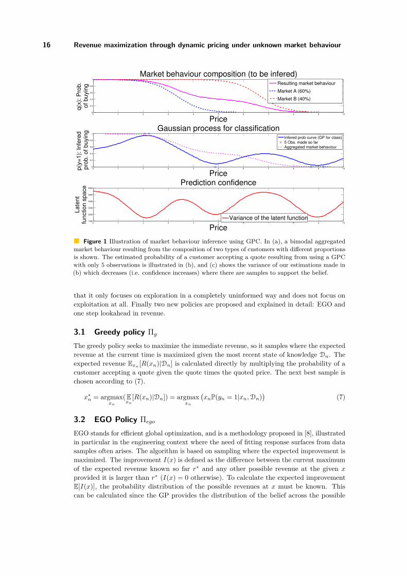
Figure 1 shows the resulting probability of buying P(y = 1) for all the prices as inferredfrom n = 5 observations using a GPC. The observations were obtained by sampling from abimodal market, which is represented by the weighted sum of the probabilities of buyingwhich are Bernoulli distributed with parameter q(x) as shown in plot (a) in Figure 1.
3 Policies to compare
The purpose of a policy is to have a rule which dictates the best action to take given ourcurrent knowledge at any given point in time, providing a systematic way of taking decisions.Under stochastic conditions an optimal policy can only guarantee up to some probabilitythat the recommended action will be the best. In general, when a process can be simulated,repeated realizations of the same process are performed in order to learn the best course ofaction. When trying to learn the market behaviour, there are two main challenges. First,the goal is to learn the transition probabilities governing the process, i.e. the distributionof the possible outcomes given the current state and action taken. This makes the processimpossible to simulate, since the probability distribution underlying the samples is unknown.And second, the value of taking an action, i.e. the obtained revenue for a given quote in thiscase, depends not only on the current state but on all the history of actions taken on whichthe current belief is based, making the process non-Markovian. This makes the problem tobe a partially observable non Markov decision process (POnMDP), which can be treated asa POMDP where the state space grows exponentially each time an action is taken [16].
This paper considers five policies. The first, called optimal policy or Πtrue, is providedonly as a benchmark and upper bound for the others since it requires the true probabilitycurve to be known. It consists simply of repeatedly quoting the price x∗ that maximizesthe expected revenue given complete information. The next two are standard policies thathave been proposed earlier (c.f. [6] for example) out of which one is the random policy Πr
and the other is the greedy policy Πg. Πr takes samples at the price x resulting from auniform distribution over the whole interval of possible prices x∗ ∼ U [x|0, xmax]. This means
SCOR’12
16 Revenue maximization through dynamic pricing under unknown market behaviour
0 1 2 3 4 5 6 7 8 9 100
0.2
0.4
0.6
0.8
1
Price
q(x
): P
rob
. o
f b
uyin
g
Market behaviour composition (to be infered)
0 1 2 3 4 5 6 7 8 9 100
0.2
0.4
0.6
0.8
1
Price
p(y
=1
): I
nfe
red
p
rob
. o
f b
uyin
g Gaussian process for classification
0 1 2 3 4 5 6 7 8 9 101000
2000
3000
4000
5000
6000
Price
La
ten
tfu
nctio
n s
pa
ce
Prediction confidence
Resulting market behaviour
Market A (60%)
Market B (40%)
Variance of the latent function
Infered prob curve (GP for class)
5 Obs. made so far
Aggregated market behaviour
Figure 1 Illustration of market behaviour inference using GPC. In (a), a bimodal aggregatedmarket behaviour resulting from the composition of two types of customers with different proportionsis shown. The estimated probability of a customer accepting a quote resulting from using a GPCwith only 5 observations is illustrated in (b), and (c) shows the variance of our estimations made in(b) which decreases (i.e. confidence increases) where there are samples to support the belief.
that it only focuses on exploration in a completely uninformed way and does not focus onexploitation at all. Finally two new policies are proposed and explained in detail: EGO andone step lookahead in revenue.
3.1 Greedy policy Πg
The greedy policy seeks to maximize the immediate revenue, so it samples where the expectedrevenue at the current time is maximized given the most recent state of knowledge Dn. Theexpected revenue Exn [R(xn)|Dn] is calculated directly by multiplying the probability of acustomer accepting a quote given the quote times the quoted price. The next best sample ischosen according to (7).
x∗n = argmaxxn
(Exn
[R(xn)|Dn]) = argmaxxn
(xnP(yn = 1|xn,Dn)
)(7)
3.2 EGO Policy Πego
EGO stands for efficient global optimization, and is a methodology proposed in [8], illustratedin particular in the engineering context where the need of fitting response surfaces from datasamples often arises. The algorithm is based on sampling where the expected improvement ismaximized. The improvement I(x) is defined as the difference between the current maximumof the expected revenue known so far r∗ and any other possible revenue at the given x
provided it is larger than r∗ (I(x) = 0 otherwise). To calculate the expected improvementE[I(x)], the probability distribution of the possible revenues at x must be known. Thiscan be calculated since the GP provides the distribution of the belief across the possible
S. Morales-Enciso and J. Branke 17
Figure 2 Two steps of the EGO policy in action are shown. Starting with (a.1), which shows theestimated probability of buying given the 3 shown data points, and (c.1) showing the confidence ofthe predictions, the expected revenue along with its confidence interval can be calculated as (b.1)illustrates. Then, using (9), the expected improvement can be calculated (d.1) and the best actionto take determined by using (10).
values, which is specified by the mean (5) and variance (6). By multiplying these two valuestimes the price x, we obtain the distribution on the expected revenue at x, which is used tocompute the expected improvement (9).
I(x) = max(r∗ − E[R(x)], 0) where r∗ = maxx(E[R(x)]) (8)
E[I(x)] =∫∞r∗I(x)P(E[R(x)])dx where P(E[R(x)]) ∼ N(E[R(x)]|µ(x), σ2(x)) (9)
Once the expected improvement E[I(x)] is known, the next best sample should be takenwhere E[I(x)] is maximized (10).
x∗ = argmaxx
(E[I(x)]) (10)
The EGO policy explicitly takes into account both information acquisition and exploitation ofwhat is believed to be the action with the highest reward. Besides, as the number of samplesincreases, the confidence intervals narrow, placing each time less weight in the explorationpart. An illustration of how this policy works is provided in Figure 2.
3.3 One step lookahead in revenue Πdp1
The one step lookahead in revenue policy proposes to sample at the maximum of the sumof the immediate expected revenue given the current observations E[R(xn)|Dn] plus theexpected revenue at the next step given the current data together with the outcome of theaction taken in the first step E[R(xn+1)|Dn∪{(xn, yn)] appropriately weighted by the current
SCOR’12
18 Revenue maximization through dynamic pricing under unknown market behaviour
belief (11). The first part of the sum corresponds to the greedy policy Πg. Since the actiontaken in step n influences our belief on the market behaviour, in order to calculate the secondpart of (11), all the possible outcomes of action xn along with their possible responses ynand the corresponding belief update, which follows from having a new sample, should betaken into account.
Exn
[R(xn)+R(xn+1)] = maxxn∈χ
{Exn
[R(xn)|Dn
]+ Exn
[maxxn+1
( Exn+1
[R(xn+1)|Dn∪{(xn, yn)}])]}
(11)
Let Pn := Pn(yn = 1|Dn) denote the estimated probability of a customer buying a productconsidering the observations available at step n, let P+
n+1 := Pn+1(yn+1 = 1|Dn ∪ {(xn, yn =1)}) denote how the estimation of the probability would update at step n + 1 had theaction xn been taken and had its outcome been a positive answer yn = 1, and let P−n+1 :=Pn+1(yn+1 = 1|Dn ∪ {(xn, yn = 0)}) denote the case where the outcome for action xn hadbeen a negative answer yn = 0.
Since there are only two possible outcomes for yn, and the revenue obtained when yn = 0is 0, only the cases with positive answers contribute to the expected revenue. However, thetwo possible outcomes must be taken into account after taking action xn, since in both casesthe belief would be updated in a different manner. Calculating the expectations given theavailable data, obtained by multiplying the price times the probability of getting a yes, weobtain:
Exn
[R(xn)+R(xn+1)] = maxxn
{xnPn+Pn max
xn+1
(xn+1P+
n+1)+(1−Pn) max
xn+1
(xn+1P−n+1
)}(12)
Finally, the next best sample according to Πdp1 is given by finding the price to be quotedsuch that it maximizes (12), which is expressed in (13)
x∗n = argmaxxn
Exn
[R(xn) +R(xn+1)] (13)
4 Implementation and results
The accumulated revenue achieved throughout a given number of quotes is considered in orderto compare the performance of the policies described above. The accumulated revenue is givenby the sum of the products of the quotes made times the response obtained: Racc = X · Y .
To see how each of the policies perform, a simulation of the process was implementedand the accumulated revenue was tracked for the first 50 samples. The market is assumedto follow a bimodal probability curve q(x) as shown in plot (a) in Figure 1. So, samplingthe market is simulated by drawing a response from a Bernoulli distribution with parameterq(x).
For each of the proposed policies, the simulation starts with 2 samples {x0, x1} ∈ [0, 10]and their response {y0, y1} ∈ {0, 1}. If there is at least one positive and one negative response,then the policies start to run. Otherwise, new samples are taken until there is at least one ofeach possible responses. This is done to ensure the inference process is not mislead from thebeginning. The new samples (before the policies start to run) are taken at min(X)/2 if Y isonly composed of zeros, or at max(X) + (10−max(X))/2 if Y is composed only of ones.
For Πtrue and Πr there is no need to perform any inference process. For the rest of thepolicies, each time a new sample is taken, the belief of the probability of buying is updated
S. Morales-Enciso and J. Branke 19
Figure 3 Performance of the five policies described in section 3. No statistically significantdifference was found in the performance for policies Πg, Πego, and Πdp1, although they all shownbetter performance compared to Πr.
by running the GPC and the price at which the next best sample is taken (x∗) is determinedby applying each policy.
For all the policies except Πdp1 the simulation was run for 100 replications, each withdifferent random seeds, but common random seeds were kept across different policies. Theaccumulated revenue for each policy and each replication was tracked along 50 samples,allowing to provide the results with confidence intervals. This is shown in Figure 3(a).Πdp1 was only ran for 50 replications and up to 25 samples because of its computationalrequirements. For clarity, the obtained results are presented in a separate plot in Figure 3(b).
After running the numerical simulations, it was found that the random policy Πr performedthe worst. This is due to the focus on constant uninformed exploration and the lack ofexploitation. Nonetheless, the simulations show no statistical difference between the other3 policies compared (Πg,Πego, and Πdp1) which seems counter intuitive. One possibleexplanation could be that no additional information is used across these 3 policies, even ifthe information available is being treated differently.
5 Conclusion and future research
In this paper, the utility of dynamic pricing used to maximize the accumulated revenueof a firm was reviewed. In particular, a memoryless market with an infinite time horizonand infinite inventory scenario was considered. A new approach to measure the marketprice sensitivity better adapted to virtual market characteristics was proposed, and twosampling policies (Πego and Πdp1) were adapted to work with non parametric inferencemodels and compared to 3 other policies commonly found in literature. It has been shownthat there is no significant difference between the proposed policies and the greedy policy.This motivates the authors to explore the design of new policies and the adaptation of knownpolicies to the described paradigm. In particular, understanding the strengths of policiesknown to outperform the greedy policy in the traditional framework can provide insight onhow to create better performing policies in the proposed setting. Future lines of researchshall include the dynamic case where the market sensitivity changes with time –hinting toconstantly consider exploration– and a delayed reward measurement case where the responseof a sample is not known until after certain time.
SCOR’12

20 Revenue maximization through dynamic pricing under unknown market behaviour
References1 Victor F. Araman and René Caldentey. Dynamic pricing for nonperishable products with
demand learning. Operations Research, 57(5):1169–1188, 2009.2 Victor F. Araman and René Caldentey. Revenue management with incomplete demand
information. Forthcoming in Encyclopedia of Operations Research, 2011.3 Yossi Aviv and Amit Pazgal. Pricing of short life-cycle products through active learning.
Working paper.4 Yossi Aviv and Amit Pazgal. A partially observed markov decision process for dynamic
pricing. Management Science, 51(9):1400–1416, 2005.5 Christopher M. Bishop. Pattern Recognition and Machine Learning (Information Science
and Statistics). Springer-Verlag New York, Inc., 1st edition, 2006.6 Alexandre X. Carvalho and Martin L. Puterman. Learning and pricing in an internet en-
vironment with binomial demands. Journal of Revenue and Pricing Management, 3(4):320– 336, 2005.
7 Guillermo Gallego and Garrett van Ryzin. Optimal dynamic pricing of inventories withstochastic demand over finite horizons. Management Science, 40(8):999–1020, 1994.
8 Donald R. Jones, Matthias Schonlau, and William J. Welch. Efficient global optimizationof expensive black-box functions. Journal of Global Optimization, 13(4):455–492, December1998.
9 P.K. Kannan and Praveen K. Kopalle. Dynamic pricing on the internet: Importance andimplications for consumer behavior. International Journal of Electronic Commerce, 5(3):63– 83, 2001.
10 Ken Littlewood. Forecasting and control of passenger bookings. American Airlines Inc,1972.
11 David J. C. Mackay. Information Theory, Inference and Learning Algorithms. CambridgeUniversity Press, 1st edition, 2003.
12 David J.C. MacKay. The evidence framework applied to classification networks. NeuralComputation, 4(5):720–736, 1992.
13 Javad Nasiry and Ioana Popescu. Dynamic pricing with loss-averse consumers and peak-endanchoring. Operations Research, 59(6):1361–1368, 2011.
14 Carl E. Rasmussen and Christopher Williams. Gaussian Processes for Machine Learning.MIT Press, 2006.
15 Jaakko Riihimäki and Aki Vehtari. Gaussian processes with monotonicity informa-tion. Journal of Machine Learning Research: Workshop and Conference Proceedings,AISTATS2010 special issue, 2010.
16 Stuart J. Russell and Peter Norvig. Artificial Intelligence: A Modern Approach. PearsonEducation, 2nd edition, 2003.
17 Troy Wolverton. Amazon backs away from test prices, 2000. http://news.cnet.com/2100-1017-245631.html (Accessed 01/04/2012).
Empirical Bayes Methods for Discrete EventSimulation Performance Measure Estimation∗
Shona Blair1, Tim Bedford1, and John Quigley1
1 Dept. of Management Science, University of Strathclyde40 George Street, Glasgow, G1 1QE, UK{shona.blair, tim.bedford, j.quigley}@strath.ac.uk
AbstractDiscrete event simulation (DES) is a widely-used operational research methodology facilitatingthe analysis of complex real-world systems. Although, generally speaking, simplicity is greatlydesirable in DES modelling applications, in many cases the nature of the underlying systemresults in simulation models which are large in scale, complex, and expensive to run. As such,the careful design and analysis of simulation experiments is essential to ensure valid and efficientinference concerning DES model performance measures. It is envisaged that empirical Bayes(EB) methods, which enable data to be pooled across a set of populations to support inference ofthe parameters of a single population, may be of use within this context. Despite this potential,EB has so far been neglected within the DES literature. This paper presents a preliminary com-putational investigation into the efficacy of EB procedures in the estimation of DES performancemeasures. The results of this investigation, and their significance, are explored. Additionally,likely directions for future research are also addressed.
1998 ACM Subject Classification I.6.8 Types of Simulation
Keywords and phrases Discrete Event Simulation, Analysis Methodology, Empirical Bayes
Digital Object Identifier 10.4230/OASIcs.SCOR.2012.21
1 Introduction and Motivation
Discrete event simulation (DES) is a powerful and flexible methodology, widely utilized in ORapplications for the design, analysis and improvement of complex, dynamic and stochasticreal-world systems. At its core, DES involves abstracting the fundamental structure of thesystem of interest and using this information to construct a computer model of the system.A process of experimentation is conducted with the computer model in order to gain insightinto and understanding of the performance of the real system. One of the key advantages ofdiscrete event simulation is its ability to incorporate a “realistic” level of system complexityinto the analysis process, when compared with the more rigid assumptions of alternativemodeling techniques; indeed, DES is frequently referred to as a “method of last resort” [9].Whilst the benefits of simple models are well understood and widely disseminated (see, forexample, [11, 13]), there are many instances when the nature of the underlying system beingstudied necessitates the use of simulation models which are large-scale, structurally complex,difficult to interpret and computationally expensive to run. As such, the careful designand analysis of simulation experiments is necessary to ensure valid and efficient inferenceconcerning model performance [8].
∗ This work was partially supported by an EPSRC CASE Studentship and SIMUL8 Corporation.
© Shona Blair, Tim Bedford, and John Quigley;licensed under Creative Commons License NC-ND
3rd Student Conference on Operational Research (SCOR 2012).Editors: Stefan Ravizza and Penny Holborn; pp. 21–30
OpenAccess Series in InformaticsSchloss Dagstuhl – Leibniz-Zentrum für Informatik, Dagstuhl Publishing, Germany
22 EB Methods for DES Performance Measure Estimation
Empirical Bayes (EB) procedures offer a structured and theoretically sound framework forthe pooling of data obtained across a set of populations to support inference concerningthe parameters of an individual population. This often enables more efficient inference insituations which feature a repeated structure, providing that sufficient “similarity” existsbetween component populations. (For a general EB reference, see [2]). It seems intuitivelyreasonable that such an approach may be of benefit in simulation model experimentation,owing to the underlying similarity between simulation model configurations. In light of thecomputational expense involved in executing simulation models (touched on above), suchincreased efficiency in estimation would likely prove highly advantageous in practice. Yet, inspite of this apparent potential, EB has so far been neglected within the simulation literature.
This paper presents the results of a preliminary computational investigation into the use ofEB procedures in the estimation of DES model performance measures. It begins, in Section2, with the presentation and brief derivation of the EB procedures which are to be applied.Then, in Section 3, the DES model selected for testing is introduced, the reasons behind thischoice outlined and certain theoretical results regarding performance measures of interestare presented. After this, in Section 4, the experimental design of the study is described,before the results are summarised in Section 5. The paper concludes, in Section 6, with somediscussion of how this research area might be further explored in the future.
2 Introducing the Empirical Bayes Procedures
Empirical Bayes procedures feature a hierarchical model structure, identical to that ofa traditional Bayesian analysis. As such, we typically have a situation in which modelparameters are themselves represented by probability distributions, termed “prior” distri-butions. In a Bayesian analysis, the prior distribution would be subjectively determined,usually elicited from subject matter experts. However, in an empirical Bayes setting thedata themselves determine the prior distribution. As mentioned in the previous section,EB methods are well-suited to applications featuring a large number of “similar” popula-tions or processes. In this situation, the data obtained from each of the populations arepooled and used to provide inference on a general prior distribution. This general priordistribution is then combined with the individual samples from each of the populationsusing standard Bayesian updating to obtain a “posterior” distribution specific to each of thepopulations. (For a detailed overview of the above theory and terminology, please refer to [2].)
EB methods have a long history, with their roots in actuarial work on credibility theory,the first major publication by Robbins [12] in 1955 and a series of landmark papers in the1970’s by Efron and Morris [4, 5, 6] (see [10] for a more detailed account of their develop-ment). However, recent years have seen a huge upsurge in the volume of EB publications.This is due predominantly to scientific advances such as microarray technology, facilitatinghigh-throughput biological screening and generating massive datasets that demand a freshapproach to statistical analysis [3]. A frequent feature of such datasets is their large numberof populations, contrasted with relatively few observations from each. Such structures, asmentioned before, are ideally suited to an empirical Bayes analysis. Indeed, many successfulapplications have been published; a recent survey being [1]. Not surprisingly, this renewedinterest has led to methodological and theoretical developments, as well as applications.
Here, however, we focus on some specific results which show particular promise in terms of
S. Blair, T. Bedford, and J. Quigley 23
their potential applicability within the context of DES model analysis. The empirical Bayesestimator shall employ is the “double-shrinkage” estimator presented in article [15]. Thisestimator assumes a normal/lognormal model of the data and its derivation is presented inthe following subsections.
2.1 AssumptionsFor i = 1, 2, . . . , p, we assume:
Xi|θi, σ2i
ind∼ N(θi, σ2i ) (1)
θiiid∼ N(µ, τ2) (2)
log σ2i
iid∼ N(µυ, τ2υ ) (3)
log(S2i /σ
2i ) iid∼ N(m,σ2
ch) (4)
where m = E[log(χ2d)] = ψ(d2 )− log(d2 ) and σ2
ch = V ar[log(χ2d)] = ψ′(d2 ), with d denoting the
degrees of freedom. Initially, we suppose that hyperparameters µ, τ2, µυ and τ2υ are known.
2.2 DerivationGiven a sample of n observations, xi, from sampling distribution (1) for population i, theprior distribution (2) on θi, and, for the moment, the additional assumption that σ2
i is known,a standard application of Bayes rule yields:
θi|xi, σ2i ∼ N(Mixi + (1−Mi)µ,Miσ
2i ), (5)
where Mi = τ2/(τ2 + σ2i /n) and xi = 1
n
∑j xij , for the posterior distribution of θi.
In such a case, we would use the posterior mean:
θi = Mixi + (1−Mi)µ, (6)
as a point estimator of θi.
However, the true population variances σ2i for i = 1, 2, . . . , p are unknown, and as with [15]
we adopt a lognormal prior (3) for σ2i , with the additional assumption (4) that S2
i /σ2i is
also lognormally distributed (with parameters selected to coincide with those of χ2d/d, the
standard distributional assumption regarding the quantity S2i /σ
2i ).
From (4), it follows that:
logS2i | log σ2
i ∼ N(m+ log σ2i , σ
2ch), (7)
and combining (3) and (7) using Bayes rule yields:
log σ2i | logS2
i ∼ N(Mυ(logS2i −m) + (1−Mυ)µυ,Mυσ
2ch), (8)
SCOR’12

24 EB Methods for DES Performance Measure Estimation
where Mυ = τ2υ/(τ2
υ + σ2ch).
As in [15], we estimate this quantity using:
σ2i = exp(Mυ(logS2
i −m) + (1−Mυ)µυ). (9)
Thus, assuming known hyperparameters, we have the estimator:
θi = Mix+ (1−Mi)µ, (10)
with Mi = τ2/(τ2 + σ2i /n), where σ2
i is as given by equation (9) above.
2.3 Estimation of HyperparametersAll that remains is the estimation of the hyperparameters µ, τ2, µυ and τ2
υ . As with [15], weadopt the following estimators.
For µυ and τ2υ , we have:
µυ = 1p
∑i
(logS2i −m) and τ2
υ = (1p
∑i
(logS2i −m)2 − σ2
ch − µ2υ)+,
from which we obtain:
Mυ = τ2υ
τ2υ + σ2
ch
and σEB,i = exp(Mυ(logS2i −m) + (1− Mυ).
To estimate µ and τ2, we use:
µ =∑i(xi/σEB,i)∑i(1/σEB,i)
and τ2 = (∑i(xi − µ)2
p)+.
Thus, the ‘double-shrinkage’ empirical Bayes point estimator is given as:
θEB,i = MEB,ixi + (1− MEB,i)µ, (11)
where MEB,i = τ2/(τ2 + σ2EB,i/n), and µ, τ2 and σ2
EB,i are as given above.
3 Introducing the DES Test Model
The purpose of this study is to evaluate the application of the EB methodology to the estim-ation of DES model performance measures. Having already introduced the EB procedures

S. Blair, T. Bedford, and J. Quigley 25
which are to be evaluated, this section aims to discuss an appropriate DES model upon whichto test the EB procedures.
The model to be used is a computer-based implementation of an M/M/1 queuing model.This simple model consists of a single-server queuing system with exponentially distributedinter-arrival and service times and a first in - first out (FIFO) queuing discipline.
Simple “artificial” DES models such as this are frequently used in research for the evaluationof DES model analysis techniques [7]. These test models offer the key advantage that theor-etical values are available for many performance measures of interest, and this knowledgegreatly facilitates the testing of output analysis methods. One criticism which can be leveledat this approach is that such models bear little resemblance to the majority of DES modelsencountered in practice (those being significantly more complex). In light of this point, itis helpful to highlight the exploratory nature of the study; it should be emphasized thatmuch of the value of this investigation lies in the issues it raises and the directions for furtherresearch which surface. This discussion is taken up again in Section 6 after the results arepresented.
For now, some relevant queuing model theory and results, extracted from [14] and used inlater sections of the paper, are presented.
3.1 M/M/1 TheoryAs discussed above, an appropriate choice of DES test model for this investigation appearsto be an M/M/1 model with a first in - first out queuing discipline. In this case, thereare only two additional model parameters which may be varied, the arrival rate, denotedby λ, and the service rate, denoted by µ. In order to simplify our analysis, we note thatthese parameters may be combined to give a single parameter, namely the traffic intensity,which uniquely specifies a particular M/M/1 configuration. The traffic intensity parameter,denoted by ρ, is given by ρ = λ
µ . We note that in future discussions, the particular M/M/1configuration will be specified solely by reference to the traffic intensity, ρ.
Our performance measure of interest will be the steady-state (or long-run) expected timein system, which we denote by W . The exact value of this quantity for any M/M/1 modelis given as a simple function of the arrival (λ) and service rate (µ) parameters, W = 1
µ−λ .This enables us to calculate the steady-state expected time in system exactly for any givenM/M/1 model configuration.
4 Experimental Design
The aim of this section is to provide an overview of the experimental design employed duringthe computational testing. Although the key points will be presented, a more comprehensivepicture of the research design may be obtained from visiting the following web address:http://personal.strath.ac.uk/shona.blair/research/SCOR2012/
Initially, it is important to mention that in this experiment, the performance of the EBestimator, θEB,i , (as given by (11) in Section 2), is evaluated relative to that of the standardestimator of a population mean, the sample mean Xi. The sample mean is most prevalentpoint estimator of DES performance measures [9]; it offers the advantage of being easily
SCOR’12

26 EB Methods for DES Performance Measure Estimation
interpretable and constitutes a convenient standard by which other methods may be compared.
In order to estimate the steady-state time in system, the test model had to be executed andtime in system data collected. The relevant details concerning this stage of the experimenta-tion are as follows:
Traffic intensities: a mesh with lower limit ρ = 0.02, upper limit ρ = 0.9 and step-sizeρ = 0.02 was used in the experiment. This resulted in 45 model configurations and gavea nice, fine grid.Number of replications: 200, 000 independent replications were made at each trafficintensity configuration to ensure sufficient data was collected.Warm-up period: a warm-up of 500 customers was used, ensuring that the model wasin steady-state prior to data collection.Run-length: a run-length of 600 customers was used. The relatively short run-length(in comparison to the warm-up period) ensured the experiment reflected possible real-lifedata collection constraints.
This scheme yields a 200, 000 by 45 data matrix, where each data value represents an aver-age time in system based on the first 100 customers after the aforementioned warm-up period.
Having obtained the necessary M/M/1 time in system data, we now discuss how this datacan be used to calculate both EB and standard estimates. In the standard setting, we simplycollect a batch of data from each traffic intensity configuration and calculate the samplemean to make inference regarding the true population mean. The only decision to be madeconcerns the size of the batch of data. In the empirical Bayes setting, however, data obtainedfrom other model configurations can be pooled to support inference of the population meanof a given configuration. Thus immediate decisions need to be made concerning the size ofthe batches to be used and the pooling strategy to be employed.
To gain as much insight as possible, a range of batch sizes were explored, from 3 to 20. Thisenabled us to understand how the batch size affected the performance of the estimationtechnique. Additionally, in terms of the pooling strategy employed, a simple two sample t-testwas conducted systematically for each pair of traffic intensity configurations to test for ho-mogeneity. This approach was adopted as it avoids subjective decisions, based on theoreticalknowledge of the system, biasing the results of the study. A range of significance levels, from0.05, 0.1, 0.15, ..., 0.95, were used to explore the relationship between pooling strategy and EBperformance. This design resulted in 342 possible combinations of batch size and significancelevel, each of which was evaluated in the course of the computational testing. For each ofthese batch size / significance level combinations, the large volume of M/M/1 data collectedpermitted the calculation of 10, 000 pairs (both EB and standard) of estimates for each ofthe 45 traffic intensities. It is thus convenient to consider two 10, 000 by 45 matrices (onefor each estimator) associated with each of the 342 batch size / significance level combinations.
To assess the performance of each estimator, the estimated values were subtracted from thetrue values, the errors squared, and the averages calculated over the 45 traffic intensities.This created, for each estimator, 10, 000 mean squared error (MSE) values. These wereaveraged, to remove the issue of stochastic variability, and the square root was taken toobtain the root mean squared error (rMSE) for each estimator. In order to gauge the relativeefficacy, the ratio of the EB rMSE over the standard rMSE was taken as our critical statistical
S. Blair, T. Bedford, and J. Quigley 27
metric of interest. Finally, note that both the M/M/1 model and the EB and standard dataanalysis procedures were implemented in Matlab R2011a and run on a standard desktop PC(Intel Core-i5, 3GHz, 8GB RAM).
5 Summary and Discussion of Experimental Results
This section of the paper briefly presents and discusses the key results obtained from theaforementioned program of experimentation. As in the previous section, we begin by notingthat a comprehensive set of numerical results and a detailed analysis may be found at thesame web address. As mentioned in the previous section, the key statistical metric of interestis the ratio of the rMSE of the EB estimator to the rMSE of the standard estimator. Thevalue of this quantity for each combination of batch size and significance level can found inTable 1 of Appendix A, which has been illustrated in Figure 1.
Figure 1 Ratio of EB rMSE to standard rMSE: This depicts the relative performance of theestimators, and how this varies with batch size and significance level. The plane at ratio= 1 enablesus to easily identify areas where the EB estimator outperforms the standard estimator.
From examination of Table 1, the most favourable value of this ratio (0.8852) was obtainedusing a batch size of 3 and a significance level of 0.4, whilst the least favourable (1.6980)occurred for batch size 5 and a significance level of 0.05. Additionally, it appears that theoptimal significance level, in terms of EB performance, is 0.4. As such, Figure 2 illustratesthe relative EB performance for this significance level over varying batch size.
6 Conclusion and Future Research
As may be seen from the results illustrated in the previous section, quantifiable benefit canbe achieved from the application of EB procedures to DES performance measure estimation.
SCOR’12
28 EB Methods for DES Performance Measure Estimation
Figure 2 rMSE ratio over varying batch size for optimal significance level.
This is a positive outcome to our pilot study which goes a significant way towards establishingthe feasibility of the application of empirical Bayes to DES model performance measureestimation. However, it is also apparent that the batch size used and the pooling strategyadopted are critical to the realization of this benefit. In this study, the decision as to whetheror not to pool model configurations was made on the outcome of a simple two sample t-test.Although there are many more options for statistical tests of homogeneity, little in the wayof formal guidance exists specifically concerning empirical Bayes pooling strategies. Moreexploration should be done on this subject with the aim of providing statistical indicators toguide practitioners in how to apply this method.
DES models exhibit great variety, differing vastly in characteristics such as purpose, struc-ture, scale, nature of input parameters and nature of output distributions. This complexityincreases the challenges involved in attempting to apply empirical Bayes to model analysisand in attempting to provide detailed guidelines enabling practitioners to make use of thismethodology. A comprehensive study evaluating the benefits of EB in relation to more“realistic” DES models forms part of our ongoing research.
Acknowledgements We would like to thank Stephen Chick for several fruitful discussionson this topic and for his involvement as external supervisor of S. Blair, and the Simul8Corporation for their technical advice and general project support.
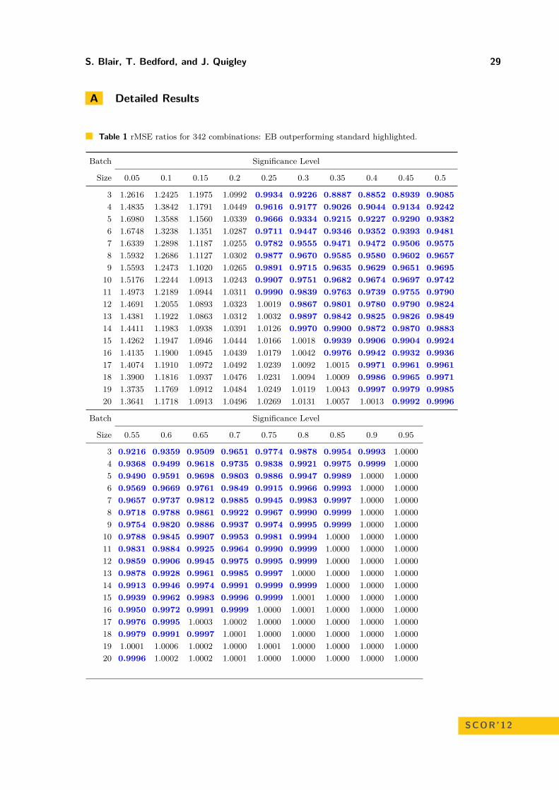
S. Blair, T. Bedford, and J. Quigley 29
A Detailed Results
Table 1 rMSE ratios for 342 combinations: EB outperforming standard highlighted.
Batch Significance Level
Size 0.05 0.1 0.15 0.2 0.25 0.3 0.35 0.4 0.45 0.5
3 1.2616 1.2425 1.1975 1.0992 0.9934 0.9226 0.8887 0.8852 0.8939 0.90854 1.4835 1.3842 1.1791 1.0449 0.9616 0.9177 0.9026 0.9044 0.9134 0.92425 1.6980 1.3588 1.1560 1.0339 0.9666 0.9334 0.9215 0.9227 0.9290 0.93826 1.6748 1.3238 1.1351 1.0287 0.9711 0.9447 0.9346 0.9352 0.9393 0.94817 1.6339 1.2898 1.1187 1.0255 0.9782 0.9555 0.9471 0.9472 0.9506 0.95758 1.5932 1.2686 1.1127 1.0302 0.9877 0.9670 0.9585 0.9580 0.9602 0.96579 1.5593 1.2473 1.1020 1.0265 0.9891 0.9715 0.9635 0.9629 0.9651 0.969510 1.5176 1.2244 1.0913 1.0243 0.9907 0.9751 0.9682 0.9674 0.9697 0.974211 1.4973 1.2189 1.0944 1.0311 0.9990 0.9839 0.9763 0.9739 0.9755 0.979012 1.4691 1.2055 1.0893 1.0323 1.0019 0.9867 0.9801 0.9780 0.9790 0.982413 1.4381 1.1922 1.0863 1.0312 1.0032 0.9897 0.9842 0.9825 0.9826 0.984914 1.4411 1.1983 1.0938 1.0391 1.0126 0.9970 0.9900 0.9872 0.9870 0.988315 1.4262 1.1947 1.0946 1.0444 1.0166 1.0018 0.9939 0.9906 0.9904 0.992416 1.4135 1.1900 1.0945 1.0439 1.0179 1.0042 0.9976 0.9942 0.9932 0.993617 1.4074 1.1910 1.0972 1.0492 1.0239 1.0092 1.0015 0.9971 0.9961 0.996118 1.3900 1.1816 1.0937 1.0476 1.0231 1.0094 1.0009 0.9986 0.9965 0.997119 1.3735 1.1769 1.0912 1.0484 1.0249 1.0119 1.0043 0.9997 0.9979 0.998520 1.3641 1.1718 1.0913 1.0496 1.0269 1.0131 1.0057 1.0013 0.9992 0.9996
Batch Significance Level
Size 0.55 0.6 0.65 0.7 0.75 0.8 0.85 0.9 0.95
3 0.9216 0.9359 0.9509 0.9651 0.9774 0.9878 0.9954 0.9993 1.00004 0.9368 0.9499 0.9618 0.9735 0.9838 0.9921 0.9975 0.9999 1.00005 0.9490 0.9591 0.9698 0.9803 0.9886 0.9947 0.9989 1.0000 1.00006 0.9569 0.9669 0.9761 0.9849 0.9915 0.9966 0.9993 1.0000 1.00007 0.9657 0.9737 0.9812 0.9885 0.9945 0.9983 0.9997 1.0000 1.00008 0.9718 0.9788 0.9861 0.9922 0.9967 0.9990 0.9999 1.0000 1.00009 0.9754 0.9820 0.9886 0.9937 0.9974 0.9995 0.9999 1.0000 1.000010 0.9788 0.9845 0.9907 0.9953 0.9981 0.9994 1.0000 1.0000 1.000011 0.9831 0.9884 0.9925 0.9964 0.9990 0.9999 1.0000 1.0000 1.000012 0.9859 0.9906 0.9945 0.9975 0.9995 0.9999 1.0000 1.0000 1.000013 0.9878 0.9928 0.9961 0.9985 0.9997 1.0000 1.0000 1.0000 1.000014 0.9913 0.9946 0.9974 0.9991 0.9999 0.9999 1.0000 1.0000 1.000015 0.9939 0.9962 0.9983 0.9996 0.9999 1.0001 1.0000 1.0000 1.000016 0.9950 0.9972 0.9991 0.9999 1.0000 1.0001 1.0000 1.0000 1.000017 0.9976 0.9995 1.0003 1.0002 1.0000 1.0000 1.0000 1.0000 1.000018 0.9979 0.9991 0.9997 1.0001 1.0000 1.0000 1.0000 1.0000 1.000019 1.0001 1.0006 1.0002 1.0000 1.0001 1.0000 1.0000 1.0000 1.000020 0.9996 1.0002 1.0002 1.0001 1.0000 1.0000 1.0000 1.0000 1.0000
SCOR’12

30 EB Methods for DES Performance Measure Estimation
References1 Y. Benjamini. Discovering the false discovery rate. Journal of the Royal Statistical Society:
Series B (Statistical Methodology), 72(4):405–416, 2010.2 B.P. Carlin and T.A. Louis. Bayesian methods for data analysis. Texts in statistical science.
CRC Press, 2009.3 B. Efron. Large-Scale Inference: Empirical Bayes Methods for Estimation, Testing, and
Prediction. Institute of Mathematical Statistics Monographs. Cambridge University Press,2010.
4 B. Efron and C. Morris. Limiting the risk of bayes and empirical bayes estimators - part ii:The empiricial bayes case. Journal of the American Statistical Society, 67:130–139, 1972.
5 B. Efron and C. Morris. Stein’s estimation rule and it competitors - an empiricial bayesapproach. Journal of the American Statistical Society, 68:117–130, 1973.
6 B. Efron and C. Morris. Dta analysis using stein’s estimator and its generalizations. Journalof the American Statistical Society, 70:311–319, 1975.
7 K. Hoad, S. Robinson, and R. Davies. Classification of discrete event simulation modelsand output: creating a sufficient model set. In Operational Research Society SimulationWorkshop 2010 (SW10), 2010.
8 J.P.C. Kleijnen, S.M. Sanchez, T.W. Lucas, and T.M. Cioppa. State-of-the-art review:A user’s guide to the brave new world of designing simulation experiments. INFORMSJournal on Computing, 17(3):263–289, 2005.
9 A.M. Law. Simulation modeling and analysis. McGraw-Hill series in industrial engineeringand management science. McGraw-Hill, 2007.
10 J.S. Maritz. Empirical Bayes methods. Methuen’s monographs on applied probability andstatistics. Methuen, 1970.
11 M. Pidd. Computer simulation in management science. Wiley, 2004.12 H. Robbins. An empirical bayes approach to statistics. In Proceedings of the Third Berke-
ley Symposium on Mathematical Statistics and Probability, pages 157–164. University ofCalifornia Press, 1955.
13 S. Robinson. Conceptual modelling for simulation part i: definition and requirements.Journal of the Operational Research Society, 59(3):278–290, 2008.
14 S.M. Ross. Introduction to Probability Models. Academic Press, 2009.15 Z. Zhao. Double shrinkage empirical bayesian estimation for unknown and unequal vari-
ances. Statistics and Its Interface, 3(4):533–541, 2010.

The Transition to an Energy Sufficient EconomyTimothy S. Mbasuen1 and Richard C. Darton2
1 Department of Engineering Science, University of OxfordOX1 3PJ, Oxford, United [email protected]
2 Department of Engineering Science, University of OxfordOX1 3PJ, Oxford, United [email protected]
AbstractNigeria is an energy-rich nation with a huge energy resource base. The country is the largestreserves holder and largest producer of oil and gas in the African continent. Despite this, onlyabout 40% of its 158 million people have access to modern energy services. Around 80% of itsrural population depend on traditional biomass. This paper presents an overview of ongoingresearch to examine energy policies in Nigeria. The aims are: 1) to identify and quantify thebarriers to sustainable energy development and 2) to provide an integrated tool to aid energypolicy evaluation and planning. System dynamics modelling is shown to be a useful tool to mapthe interrelations between critical energy variables with other key sectors of the economy, and forunderstanding the energy use dynamics (impact on society and the environment). It is found thatthe critical factors are burgeoning population, lack of capacity utilisation, and inadequate energyinvestments. Others are lack of suitably trained manpower, weak institutional frameworks, andinconsistencies in energy policies. These remain the key barriers hampering Nigeria’s smoothtransition from energy poverty to an energy sufficient economy.
1998 ACM Subject Classification I.6 Simulation and Modelling
Keywords and phrases energy sufficiency, energy policy, policy evaluation, economic planning,modelling
Digital Object Identifier 10.4230/OASIcs.SCOR.2012.31
1 Introduction
Nigeria, though an ‘energy-rich’ country falls within the category of countries suffering from‘energy poverty’ as defined by the UN [1]. The country is the largest reserves holder andlargest producer of oil and gas in Africa; yet, only about 40% of its total population haveaccess to modern energy services [2]. Around 80% of its rural population depend almostwholly on traditional biomass for their energy needs [2]. The country’s energy industryremains inefficient in meeting the energy needs and aspirations of its customers. This isevident in the dismal performance of the industry in terms of service delivery and per capitaoutput.
For instance, in spite of its enormous oil and gas activities, the petroleum industrycurrently provides less than 15% of the country’s GDP [3, 4]. Similarly, its GDP per capitaand electricity consumption per capita remains among the lowest even in Sub-SaharanAfrica-behind Angola and Ghana [5]. Persistent energy crisis has significantly weakened theindustrialisation of the country, and grossly undermines the sustainable development agendaof the government.
© Timothy S. Mbasuen and Richard C. Darton;licensed under Creative Commons License NC-ND
3rd Student Conference on Operational Research (SCOR 2012).Editors: Stefan Ravizza and Penny Holborn; pp. 31–42
OpenAccess Series in InformaticsSchloss Dagstuhl – Leibniz-Zentrum für Informatik, Dagstuhl Publishing, Germany

32 The Transition to an Energy Sufficient Economy
A review of technical and policy documents [5, 6, 7, 8, 9], and discussions with keypolicymakers in the energy industry reveal that the most serious challenges hindering thecountry from meeting its energy aspirations include: burgeoning population, lack of capacityutilisation (at all levels), and inadequate energy investments. Others are corruption, lackof suitably trained manpower, weak institutional frameworks, and inconsistencies in energypolicies [6]. These remain the key barriers hampering Nigeria’s smooth transition from energypoverty to an energy sufficient economy.
Despite these enormous challenges, there is still the lack of appropriate policy evaluationand planning tools to aid informed decision making process. The only recognised structuredtools that have so far been attempted in planning and examining energy policies in thecountry are the IAEA’s1 MAED2 and WASP3[10]. While these models are capable of givingvaluable insights into analysis of energy demand and supply in an economy, they are notable to account for other dynamics relating to society and the environment, since they arelargely based on a static economic modelling approach.
Elsewhere in the world, particularly in the transition and other developing economies,system dynamics models have been used to support energy policy evaluation and economicplanning. Notable among recent examples is the successful application of the T21 modelframework of the Millennium Institute (MI) in China, Denmark, the Balkans, and Guyana[11]. In the African continent and the Caribbean, specific examples include Ghana, Mali,Malawi, Mozambique, and Jamaica [11]. The success stories for these countries also serve asa motivation for developing a similar model for Nigeria.
In recognition of the overall long-term energy security and sustainability implications ofthe current energy/economic crises, the government has embarked on a policy of vigorousreforms to improve the situation. This paper presents an overview of ongoing research beingundertaken to examine energy policies in Nigeria using system dynamics modelling andmulti-criteria analysis. The aims are: 1) to identify and quantify the barriers to sustainableenergy development and 2) to provide an integrated and holistic tool to aid energy policyevaluation and economic planning for the country.
2 The Barriers to Sustainable Energy Development in Nigeria
As an emerging economy, Nigeria has faced a number of development challenges. In itsenergy industry for example, there is currently a massive gap between energy demand andsupply. The inability of the nation to effectively develop its vast energy resources, to improvethe economic and the social wellbeing of its people is attributed to a range of barriers. Themost fundamental of these factors are considered in this discussion.
2.1 Burgeoning PopulationNigeria’s population has continued to grow over the last five decades; the total populationwas last reported at 158.32 million people in 2010, up from 110.00 million in 1995 [12]. Inspite of birth control mechanisms currently available in the country-leading to a steadydecline in birth rates, it is still expected that the country’s overall population will continueto grow into the future. The implication however, is that a continuous rise in population
1 International Atomic Energy Agency.2 Model for Analysis of Energy Demand: (for evaluation of future energy demand).3 Wien Automatic System Planning: (for finding optimal expansion plans for power generating systems).

T.S. Mbasuen and R.C. Darton 33
means energy demand is likely to increase, even faster. Such a rise in population will notonly constitute a serious barrier to energy poverty reduction strategy of the government, butwill equally impede the overall human development process of the nation.
2.2 Lack of Capacity Utilisation
Despite its diverse energy resource base as illustrated in Table 1, the overall capacityutilisation of energy resources (defined in Btoe4) in the country remains very dismal. Thekey challenges include: lack of awareness, lack of skilled manpower, inadequate funding, andtechnological barriers [2, 13]. Lack of awareness in this context is taken to denote a lowperception of the benefits of renewable and decentralised energy options. Furthermore, theinability of government to adopt state-of-the art energy efficient technologies such as CHCP5
in its energy development strategies remains a serious impediment to sustainable energydevelopment.
Table 1 Nigeria’s Proved Conventional Energy Reserves at 2011 [7, 14].
SNo Resource type Reserve Energy value (Btoe) Lifespan (Years)1 Crude oil 37.2 billion barrel 5.431 43.12 Natural gas 187 trillion scf 4.485 1143 Coal and lignite 2.175 billion tonnes 1.512 794 Tar sands 40.6 billion barrel equiv. 5.928 505 Uranium Not yet quantified - -
2.3 Inefficient Energy Supply Infrastructure
In spite of a relatively low energy consumption profile overall (Figure 1a), the in-countryenergy supply capability is still very depressing. For instance, the country maintains fourrefineries with a combined crude processing capacity of 450 000 barrels/day; yet, none ofthe refineries has ever operated to optimal capacity [14]. Over the last 15 years, some ofthe refineries operated at 0 and 30% capacity, leaving a shortfall of about 85% to be metby imports [14]. In the upstream sub sector, the country is known to substantially flare
(a) Oil Production and Consumption (b) Gas Flaring (2010)
Figure 1 Nigeria Oil Production & Consumption and Gas Flaring.
4 Billion tonnes of oil equivalent (authors’ computations).5 Combined Heat-Cooling and Power.
SCOR’12

34 The Transition to an Energy Sufficient Economy
its natural gas for lack of infrastructure to market it. According to NOAA6 [15], about536 billion scf of natural gas was flared in the country in year 2010 (shown in Figure 1b).In monetary terms, the NNPC7 estimates that gas flaring8 costs the nation in average 2.5billion US dollars per year in lost revenue [7]. While this is largely attributed to technologicalchallenges, the problem is reinforced by inadequate funding, poor maintenance culture, andinconsistent energy policies.
2.4 Inadequate Energy InvestmentsAnother barrier to effective development and utilisation of energy resources in Nigeria isinadequate funding. In the power sector for instance, government proposed to invest a totalof 5.8 billion US dollars (for the period 2005 - 2013) [6]. This amount obviously, is inadequate,in view of the deplorable state of the electricity sub sector, and the high take-off investmentfunds required for developing renewable technologies.
The proposed public sector investment in the oil and gas upstream and downstream isapproximately 3.8 billion US dollars [6]. In realistic terms, this amount is only sufficient tobuild one modern refinery. It implies therefore, that such meagre investment proposals canhardly make any noticeable difference, except more robust funding schemes are adopted.
2.5 Lack of Suitably Trained ManpowerThe population structure of Nigeria provides a solid base for assessing availability and thequality of human capital and labour force necessary to transform the energy industry and theentire economy of the country. Review of energy industry and government reports [5, 6, 7],as well as historical data [14, 16] reveal that majority of the country’s labour force are eitherunskilled or semiskilled. These categories of workforce apparently, are unlikely to change theeconomic fortunes of the country. Further discussions on this barrier are considered in themodel representation section of this report.
2.6 Weak Institutional FrameworksMany established energy institutions are unable to demonstrate focused regulatory andmanagement capability required to improve energy development activities in the country. Forexample, the NNPC and DPR9 have been proposing an end to gas flaring in the country forseveral years, but the deadlines to implement the policies has been repeatedly postponed [14].Similarly, the loss of about 35 - 48% of electricity generated in the country to transmissionand distribution losses is largely blamed on inability of the PHCN10, to perform maintenanceand upgrade of electricity supply infrastructure [2, 6]. These and many similar institutionalchallenges remain the barriers to smooth transformation of the nation’s energy industry.
According to Transparency International’s 2011 Corruption Perception Index (CPI),Nigeria is ranked 143 out of 182 countries for corruption-behind other African countries suchas Botswana, Rwanda, and Namibia [17]. The evidence and impact of corruption can beseen in different sectors of the Nigerian economy. For example, ‘Trading Economics’ noted
6 National Oceanic Atmospheric Administration.7 Nigerian National Petroleum Corporation.8 Gas Flaring in the context of oil production simply refers to the burning off (into the atmosphere) ofnatural gas associated with crude oil.
9 Department of Petroleum Resources.10Power Holding Company of Nigeria.

T.S. Mbasuen and R.C. Darton 35
that Nigeria is one of the most advanced economies in Africa with average GDP growthof about 7.7% (as of last quarter of 2011), and about 95% foreign exchange earnings fromoil and gas exports [18]. Yet, agriculture remains the main source of revenue to 2/3 of itspopulation; while more than 50% of Nigerians still live in extreme poverty [12, 18]. Suchdismal performance among other crucial issues is largely ascribed to corruption in bothpublic and private sectors, and the lack of proper institutional frameworks for dealing with it[6, 14, 18].
However, the Economic and Financial Crimes Commission (EFCC) and other similarbodies in the country are working to address these issues [8, 9]. More detailed ‘quantitative’discussions on corruption in the country is captured elsewhere in the model under ‘GovernmentRevenue and Expenditure’.
3 Energy Policy Reforms
As revealed in the foregoing, the current picture of energy development in Nigeria is marredby a number of challenges. It is against this backdrop that government has embarkedon ambitious policy plans to improve the nation’s energy and economic situation. Oneof the desired outcomes is to provide secure and sustainable energy access to its teemingpopulation-particularly the rural population. To achieve this, the policy thrust indicatesenhanced development of both conventional and renewable energy resources.
4 Current Study Objective and Methodology
4.1 ObjectiveThe focus of this study is to develop a system dynamics (SD) model that maps the interrela-tions between critical energy variables (in Nigeria) and its impact on the three sustainabilitydomains: the society, the economy, and the environment. The aims are: 1) to combine the SDmodel with a multi-criteria analysis (MCA) technique to examine energy policies, with theoverall intent of identifying and quantifying the barriers to sustainable energy development.2) To provide an integrated and holistic policy evaluation and economic planning tool to aidinformed decision making in the country.
4.2 MethodologyThis study consists of four major phases as follows:
Phase I : the first phase of the study (October 2010 – June 2011) involved critical review ofliterature on sustainability concepts; assessment tools and methodologies; current approachesto policy development and policy evaluation; and critique of the Nigerian energy system. Thesystem dynamics methodology was found to be a useful approach for building an economy-wide dynamic model, which when combined with a simple, stakeholder-focused MCA methodsuch as SMART11, would provide a robust framework for analysing both the technical andsocial dynamics of the energy system.
Phase II : the second phase of the research (July 2011 – December 2011) developed atheoretical framework that enables integration of the proposed SD model with the chosenMCA technique. The idea was that combining an SD simulation model with a ‘social-oriented’
11 Simple Multi-Attribute Ranking Technique.
SCOR’12

36 The Transition to an Energy Sufficient Economy
MCA model would result into a more rigorous and inclusive approach to exploring energypolicies. The role of the MCA method is to account for stakeholder perspectives and todeal with issues of trade-offs. More importantly, it will aid us in making choices betweencompeting policy alternatives.
Phase III : the third phase of the study (January 2012 – September 2012) is focusedon data gathering, and building the proposed SD simulation model. The overall modelconceptualisation and formulation process had commenced during the second phase of theresearch, with a few targeted Nigerian stakeholder contacts/discussions.
Phase IV : the fourth and last phase of the research (October 2012 – September 2013),will focus on full model verification, and a demonstration of how the SD simulation modeland SMART value model can work together, for effective policy valuation. The process willinitially involve systematic model calibration with historical data. In addition, the integratedmodel will be reviewed with experts in the ministries of energy and national planning (thepotential users of the model), who earlier provided inputs in developing the model.
The verification process is also expected to be iterative, as it will largely involve presentingthe model output to stakeholders, getting feedback, updating and representing it for additionalcomments. The idea is to ensure the most comprehensive input possible from experts andpolicymakers.
5 The Energy Dynamics Model
5.1 Model PurposeIn broad terms, the purpose of the proposed ‘Energy Dynamics Model’ is to map theinterrelations that characterise the overall energy situation of Nigeria, and to serve as a‘baseline’ from where alternative policies aimed at improving the social, the economic, andthe environmental conditions of the country can be tested. In a specific sense, the modelseeks to answer the overarching research question: how and over what timescale can Nigeriamake a smooth transition from ‘energy poverty’ to an ‘energy sufficient’ economy?
5.2 Dynamical Hypothesis: a High Level MapA high level map-HLM (Figure 2), was configured to encapsulate the overall model structureconsidered for the study. The HLM also serves as a dynamical hypothesis, which governsthe development of the final model (using vensim™). In the HLM, there are four criticalfoci: energy resource (availability), energy demand (management), energy production/supply(efficiency), and energy financing (investment). The HLM hypothesises that these criticalenergy variables need to be broadly in balance, if Nigeria’s transition to an energy sufficienteconomy is to be achieved smoothly. The elements are in a dynamic equilibrium, such thatany distortion in their balance is likely to create ripple effects on the entire economy.
As illustrated in the map, availability (centre upper left corner) of viable primary energyresources (top left corner) is the first step towards ensuring energy security for the nation.The supply (centre lower right corner) of these resources is triggered by the demand (centreupper right corner) for energy to power and sustain the economy (top right corner). However,a sustainable production12 (centre lower left corner) of the energy resources is only feasible
12Energy ‘production’ in this sense is distinguished from ‘supply’ in that by production, we refer to actualprocess of extracting/converting primary energy resources; while supply refers to the process of makingenergy products available (including domestic/exports).
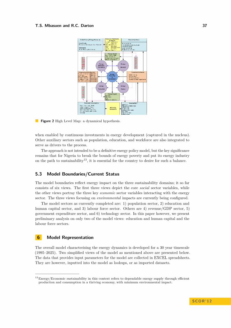
T.S. Mbasuen and R.C. Darton 37
Figure 2 High Level Map: a dynamical hypothesis.
when enabled by continuous investments in energy development (captured in the nucleus).Other auxiliary sectors such as population, education, and workforce are also integrated toserve as drivers to the process.
The approach is not intended to be a definitive energy policy model, but the key significanceremains that for Nigeria to break the bounds of energy poverty and put its energy industryon the path to sustainability13, it is essential for the country to desire for such a balance.
5.3 Model Boundaries/Current Status
The model boundaries reflect energy impact on the three sustainability domains; it so farconsists of six views. The first three views depict the core social sector variables, whilethe other views portray the three key economic sector variables interacting with the energysector. The three views focusing on environmental impacts are currently being configured.
The model sectors as currently completed are: 1) population sector, 2) education andhuman capital sector, and 3) labour force sector. Others are 4) revenue/GDP sector, 5)government expenditure sector, and 6) technology sector. In this paper however, we presentpreliminary analysis on only two of the model views: education and human capital and thelabour force sectors.
6 Model Representation
The overall model characterising the energy dynamics is developed for a 30 year timescale(1995–2025). Two simplified views of the model as mentioned above are presented below.The data that provides input parameters for the model are collected in EXCEL spreadsheets.They are however, inputted into the model as lookups, or as imported datasets.
13Energy/Economic sustainability in this context refers to dependable energy supply through efficientproduction and consumption in a thriving economy, with minimum environmental impact.
SCOR’12
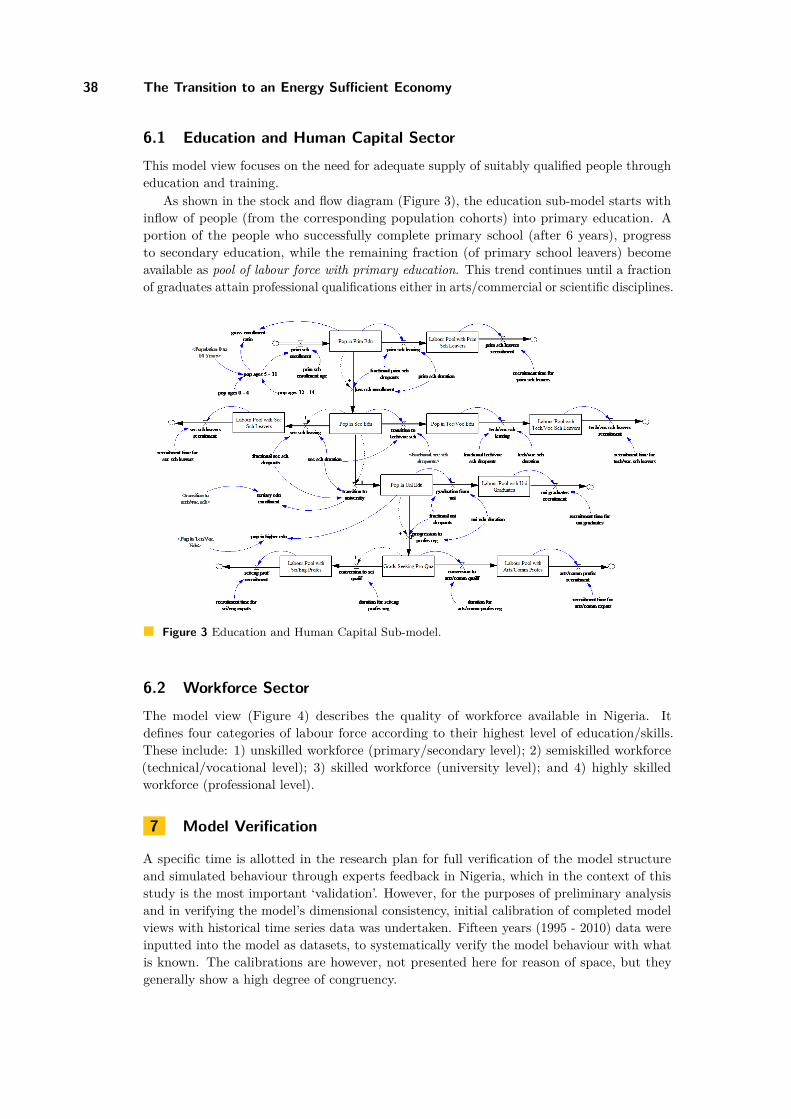
38 The Transition to an Energy Sufficient Economy
6.1 Education and Human Capital SectorThis model view focuses on the need for adequate supply of suitably qualified people througheducation and training.
As shown in the stock and flow diagram (Figure 3), the education sub-model starts withinflow of people (from the corresponding population cohorts) into primary education. Aportion of the people who successfully complete primary school (after 6 years), progressto secondary education, while the remaining fraction (of primary school leavers) becomeavailable as pool of labour force with primary education. This trend continues until a fractionof graduates attain professional qualifications either in arts/commercial or scientific disciplines.
Figure 3 Education and Human Capital Sub-model.
6.2 Workforce SectorThe model view (Figure 4) describes the quality of workforce available in Nigeria. Itdefines four categories of labour force according to their highest level of education/skills.These include: 1) unskilled workforce (primary/secondary level); 2) semiskilled workforce(technical/vocational level); 3) skilled workforce (university level); and 4) highly skilledworkforce (professional level).
7 Model Verification
A specific time is allotted in the research plan for full verification of the model structureand simulated behaviour through experts feedback in Nigeria, which in the context of thisstudy is the most important ‘validation’. However, for the purposes of preliminary analysisand in verifying the model’s dimensional consistency, initial calibration of completed modelviews with historical time series data was undertaken. Fifteen years (1995 - 2010) data wereinputted into the model as datasets, to systematically verify the model behaviour with whatis known. The calibrations are however, not presented here for reason of space, but theygenerally show a high degree of congruency.
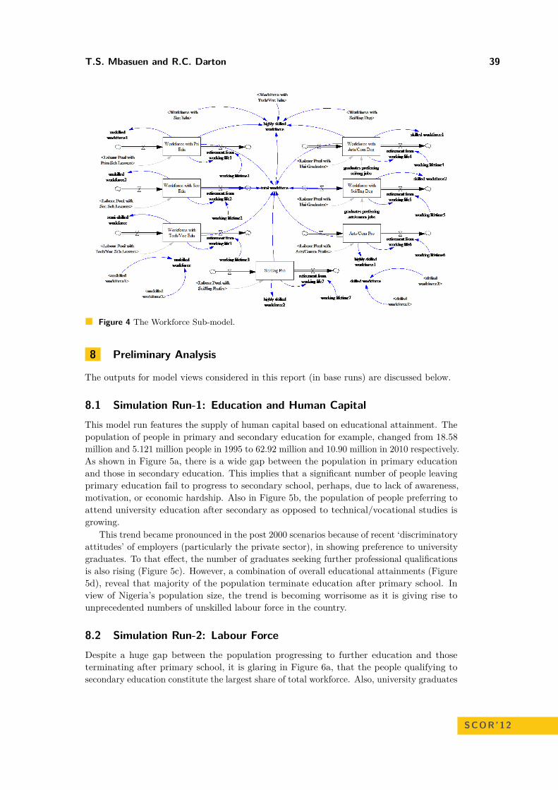
T.S. Mbasuen and R.C. Darton 39
Figure 4 The Workforce Sub-model.
8 Preliminary Analysis
The outputs for model views considered in this report (in base runs) are discussed below.
8.1 Simulation Run-1: Education and Human CapitalThis model run features the supply of human capital based on educational attainment. Thepopulation of people in primary and secondary education for example, changed from 18.58million and 5.121 million people in 1995 to 62.92 million and 10.90 million in 2010 respectively.As shown in Figure 5a, there is a wide gap between the population in primary educationand those in secondary education. This implies that a significant number of people leavingprimary education fail to progress to secondary school, perhaps, due to lack of awareness,motivation, or economic hardship. Also in Figure 5b, the population of people preferring toattend university education after secondary as opposed to technical/vocational studies isgrowing.
This trend became pronounced in the post 2000 scenarios because of recent ‘discriminatoryattitudes’ of employers (particularly the private sector), in showing preference to universitygraduates. To that effect, the number of graduates seeking further professional qualificationsis also rising (Figure 5c). However, a combination of overall educational attainments (Figure5d), reveal that majority of the population terminate education after primary school. Inview of Nigeria’s population size, the trend is becoming worrisome as it is giving rise tounprecedented numbers of unskilled labour force in the country.
8.2 Simulation Run-2: Labour ForceDespite a huge gap between the population progressing to further education and thoseterminating after primary school, it is glaring in Figure 6a, that the people qualifying tosecondary education constitute the largest share of total workforce. Also, university graduates
SCOR’12
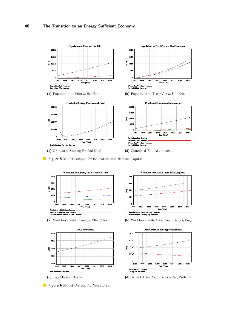
40 The Transition to an Energy Sufficient Economy
(a) Population in Prim & Sec Edu (b) Population in Tech/Voc & Uni Edu
(c) Graduates Seeking Profsnl Qual (d) Combined Edu Attainments
Figure 5 Model Output for Education and Human Capital.
(a) Workforce with Prim/Sec/Tech/Voc (b) Workforce with Arts/Comm & Sci/Eng
(c) Total Labour Force (d) Skilled Arts/Comm & Sci/Eng Profsnls
Figure 6 Model Output for Workforce.
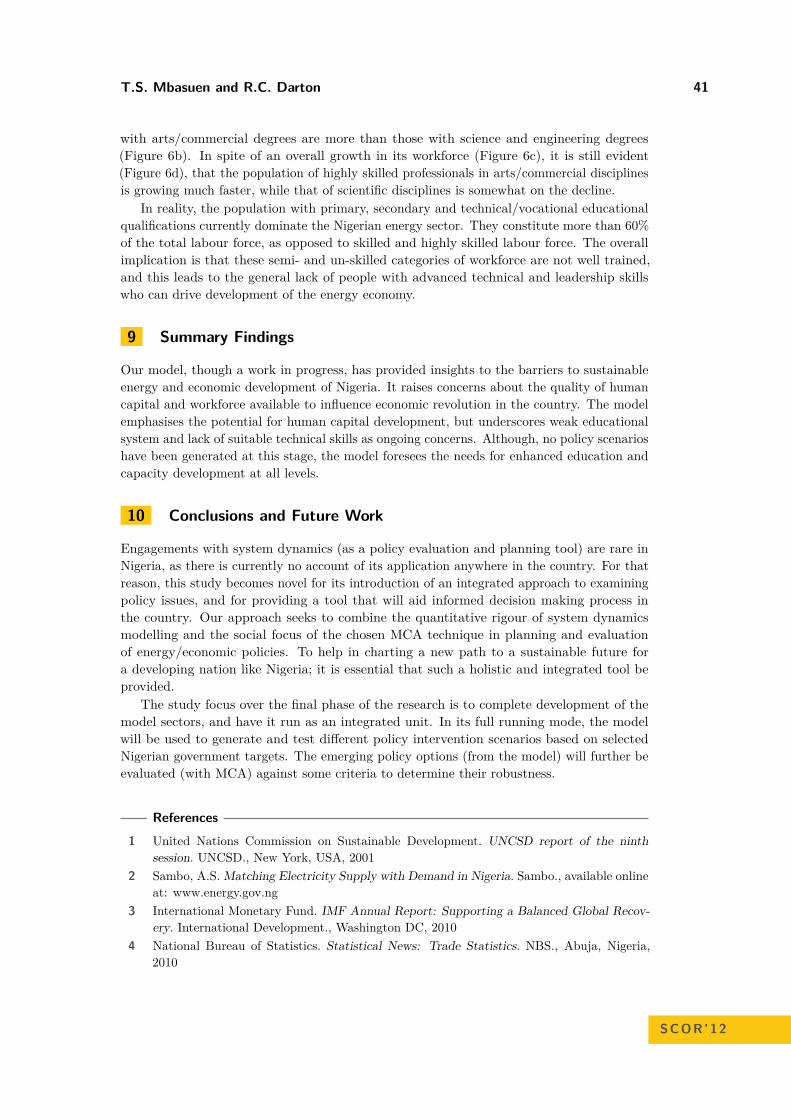
T.S. Mbasuen and R.C. Darton 41
with arts/commercial degrees are more than those with science and engineering degrees(Figure 6b). In spite of an overall growth in its workforce (Figure 6c), it is still evident(Figure 6d), that the population of highly skilled professionals in arts/commercial disciplinesis growing much faster, while that of scientific disciplines is somewhat on the decline.
In reality, the population with primary, secondary and technical/vocational educationalqualifications currently dominate the Nigerian energy sector. They constitute more than 60%of the total labour force, as opposed to skilled and highly skilled labour force. The overallimplication is that these semi- and un-skilled categories of workforce are not well trained,and this leads to the general lack of people with advanced technical and leadership skillswho can drive development of the energy economy.
9 Summary Findings
Our model, though a work in progress, has provided insights to the barriers to sustainableenergy and economic development of Nigeria. It raises concerns about the quality of humancapital and workforce available to influence economic revolution in the country. The modelemphasises the potential for human capital development, but underscores weak educationalsystem and lack of suitable technical skills as ongoing concerns. Although, no policy scenarioshave been generated at this stage, the model foresees the needs for enhanced education andcapacity development at all levels.
10 Conclusions and Future Work
Engagements with system dynamics (as a policy evaluation and planning tool) are rare inNigeria, as there is currently no account of its application anywhere in the country. For thatreason, this study becomes novel for its introduction of an integrated approach to examiningpolicy issues, and for providing a tool that will aid informed decision making process inthe country. Our approach seeks to combine the quantitative rigour of system dynamicsmodelling and the social focus of the chosen MCA technique in planning and evaluationof energy/economic policies. To help in charting a new path to a sustainable future fora developing nation like Nigeria; it is essential that such a holistic and integrated tool beprovided.
The study focus over the final phase of the research is to complete development of themodel sectors, and have it run as an integrated unit. In its full running mode, the modelwill be used to generate and test different policy intervention scenarios based on selectedNigerian government targets. The emerging policy options (from the model) will further beevaluated (with MCA) against some criteria to determine their robustness.
References
1 United Nations Commission on Sustainable Development. UNCSD report of the ninthsession. UNCSD., New York, USA, 2001
2 Sambo, A.S. Matching Electricity Supply with Demand in Nigeria. Sambo., available onlineat: www.energy.gov.ng
3 International Monetary Fund. IMF Annual Report: Supporting a Balanced Global Recov-ery. International Development., Washington DC, 2010
4 National Bureau of Statistics. Statistical News: Trade Statistics. NBS., Abuja, Nigeria,2010
SCOR’12
42 The Transition to an Energy Sufficient Economy
5 Central Bank of Nigeria. Annual Reports and Statement of Accounts. CBN., Abuja, Nigeria,2009
6 Federal Ministry of National Planning. Nigeria Vision 20:2020 First Implementation Plan(2010 - 2013). FMNP., Abuja, Nigeria, 2010
7 Nigerian National Petroleum Corporation. Oil and Gas Statistics: Annual Statistical Bul-letin. NNPC., Abuja, Nigeria, 2011
8 Economic and Financial Crimes Commission. Fighting Corruption in Nigeria. EFCC., avail-able online at: www.efccnigeria.org/
9 Independent Corrupt Practices and Other related Offences Commission. Fighting Corrup-tion in Nigeria. ICPC., available online at: www.icpc.gov.ng/
10 Sambo, A. S., Iloeje, O. C., Ojosu, J. O., Olayande, J. S., Yusuf, A. O. Nigeria’s Experienceon the Application of IAEA’s Energy Models (MAED & WASP) for National EnergyPlanning. Korea Atomic Energy Research Institute, Daejon, Korea, 2006
11 Millennium Institute. T21 Models, Papers and Newsletters. MI., available online at:www.millennium-institute.org/resources/elibrary/index.html
12 United Nations Development Programme. Human Development Report. UNDP., Washing-ton DC, 2010
13 Global Network on Energy for Sustainable Development. Renewable Energy Technologiesand Poverty Alleviation: Overcoming Barriers and Unlocking Potentials. GNESD., avail-able online at: www.gnesd.org/publications.htm
14 US Energy Information Administration. Country Analysis Briefs: Nigeria. EIA Energy andMining Report., Washington DC, 2011
15 National Oceanic and Atmospheric Administration. Global Gas Flaring Country Data. Na-tional Geographical Data Center., USA, 2010
16 IBRD/World Bank. Africa Development Indicators 2010. IBRD., Washington DC, 201017 Transparency International. Countries Ranking: Corruption Perception Index 2011. TI.,
available online at: www.transparency.org18 Trading Economics. Indicators: Nigeria GDP Growth Rate. TE., available online at:
www.tradingeconomics.com/nigeria/gdp-growth
Can online trading algorithms beat the market?An experimental evaluationJaveria Iqbal1, Iftikhar Ahmad1, and Günter Schmidt1,2
1 Chair of Information and Technology ManagementUniversity of Saarland, Germany
2 Department of Statistical SciencesUniversity of Cape Town, South Africa{ji,ia,gs}@itm.uni-sb.de
AbstractFrom experimental evaluation, we reasonably infer that online trading algorithms can beat themarket. We consider the scenario of trading in financial market and present an extensive ex-perimental study to answer the question “Can online trading algorithms beat the market?”. Weevaluate the selected set of online trading algorithms on DAX30 and measure the performanceagainst buy-and-hold strategy. In order to compute the experimentally achieved competitive ra-tio, we also compare the set of algorithms against an optimum offline algorithm. To add furtherdimensionality into experimental setup, we use trading periods of various lengths and apply anumber of evaluation criteria (such as annualized geometric returns, average period returns andexperimentally achieved competitive ratio) to measure the performance of algorithms in shortvs. long term investment decisions. We highlight the best and worst performing algorithms anddiscuss the possible reasons for the performance behavior of algorithms.
1998 ACM Subject Classification F.2 Analysis of Algorithms and Problem Complexity
Keywords and phrases Online Algorithms, Experimental Evaluation, Competitive Analysis
Digital Object Identifier 10.4230/OASIcs.SCOR.2012.43
1 Introduction
The major concern of an investor (both individual and corporate) in financial market is theprofitability of the underlying trading strategy. As financial markets are highly volatile andrisky, an investor wants to ensure that the trading strategy that he/she relies on, is profitableand provides better returns in unforeseen circumstances. Performance evaluation of thetrading strategies is required to ensure that the selected strategies are thoroughly tested inreal world scenario. Trading in financial markets is based on the principle of maximizing thedifference between selling and buying, i.e., buying at minimum possible price and selling atmaximum possible price. However, as the investor (henceforth called as player) cannot seethe future prices, his decision is based on limited knowledge.
Online algorithms can be used to support trading decisions in financial markets wherecomplete knowledge about future is not available. Online algorithms are based on theparadigm that the player has no knowledge about future and every decision the algorithmmakes is based on the current knowledge of the algorithm. Online algorithms are evaluatedthrough competitive analysis paradigm. Competitive analysis is used to measure the perform-ance of an online algorithm against an optimum offline algorithm. Let P be a maximizationproblem and I be the set of all input instances, ON be an online algorithm for problem P
© Javeria Iqbal, Iftikhar Ahmad, and Günter Schmidt;licensed under Creative Commons License NC-ND
3rd Student Conference on Operational Research (SCOR 2012).Editors: Stefan Ravizza and Penny Holborn; pp. 43–52
OpenAccess Series in InformaticsSchloss Dagstuhl – Leibniz-Zentrum für Informatik, Dagstuhl Publishing, Germany
44 Can online trading algorithms beat the market?
and ON(I) be the performance of algorithm ON on input instance I ∈ I. Let OPT be anoptimum offline algorithm for the same problem P , ON is said to be c-competitive if ∀I ∈ I
ON (I) ≥ 1c· OPT (I). (1)
We consider a set of online algorithms for trading and evaluate them from empirical per-spective by executing the set of algorithms on real world. We evaluate the performance ofalgorithms using different lengths of trading periods (10, 20, 60, 130 and 260 days) and use avariety of evaluation measures such as annualized geometric returns (AGR), average periodreturn (APR) and experimentally achieved competitive ratio (ce) to evaluate the selectedset of online algorithms.
Definitions: We present a set of basic terms and definitions with reference to onlinetrading algorithms.
i. Transaction: A transaction is either selling or buying of an asset.ii. Trade: A trade consists of two transactions, one is buying and one is selling. The number
of trading periods in an investment horizon is represented by P .iii. Investment Horizon: The total time duration in which all transactions are carried out.
The investment horizon can be divided into one or more time segments for trading.iv. Duration (T ): The length of a trading period.v. Offered Price (qt): The offered price on day t.vi. Upper Bound (M): The upper bound on possible offered prices during the trading period.vii. Lower Bound (m): The lower bound on possible offered prices during the trading period.viii. Amount Converted (st): Specifies which fraction of the amount available (e.g. wealth) is
to be converted at price qt on day t, with 0 ≤ st ≤ 1.
2 Literature Review
In this section, we briefly describe different performance evaluation techniques for onlinealgorithms and provide a short review of the literature in relation to experimental analysisof different trading strategies.
The performance of online algorithms are analyzed from three different perspectives,Bayesian Analysis assumes that the input instance is drawn from a known probabilitydistribution and expected performance of the algorithm is investigated on the assumedprobability distribution, Competitive Analysis compares the performance of online algorithmsagainst that of optimum offline algorithm, and Experimental Analysis uses the back testingtechnique to evaluate the performance of online algorithm on real world (as well as synthetic)data. Each of these techniques has its own limitations and drawbacks. The Bayesiananalysis is considered to be too optimistic and relies heavily on underlying distribution.The competitive analysis is criticized to be too pessimistic as online algorithm is comparedwith an optimum offline algorithm which has complete knowledge about the future, thusexperimental analysis can be used as a useful tool in conjunction with worst case competitiveanalysis to evaluate the performance of online algorithms and to measure the disparitybetween theoretical and real world performance of online algorithms.
The experimental analysis of online trading algorithms is not widely addressed in theliterature. Mohr and Schmidt [7] presented an empirical study where the reservation pricealgorithm of El-Yaniv et al. [2] is compared with buy-and-hold (BH). Schmidt et al. [9]evaluated the reservation price algorithm and threat based algorithm [2] to dollar average
J. Iqbal, I. Ahmad, and G. Schmidt 45
strategy (DAS) and BH. However, there is no such study which considers a broader set ofonline algorithms for trading and evaluate them extensively on real world dataset.
The experimental evaluation of heuristics trading algorithms has received considerableattention from researchers. In these studies BH is used as a benchmark for comparingdifferent strategies. Due to space constraint the details cannot be included and the reader isreferred to [1, 4, 6, 8, 10, 11].
3 Online Trading Algorithms
We briefly discuss the set of online trading algorithms. The proof of competitive ratio andoptimality of algorithm is left out due to space constraint and the reader is referred tocorresponding research papers. The online trading algorithms are broadly classified as NonPreemptive and Preemptive algorithms.
3.1 Non Preemptive AlgorithmsIn non preemptive algorithms (also referred to as reservation price algorithms), the playerinvests (buys or sells) his whole wealth at one point of time in investment horizon. Theplayer computes a reservation price and compares each offered price with reservation price.A reservation price is the maximum(minimum) price which a player will accept for buying(selling). The player takes a buy decision and invests at the offered price if it is less or equalthan the pre-computed reservation price, and a sell decision is taken when the offered price isgreater (or equal) than the pre-computed reservation price. We discuss algorithms presentedby El-Yaniv et al. [2] and Kao and Tate [3] and BH strategy.
3.1.1 El-Yaniv et al. reservation price algorithmEl-Yaniv et al. [2] presented reservation price algorithm based on the assumption that thelower and upper bound of offered price m and M are known to the player. El-Yaniv et al.presented the strategy for max-search (sell) problem. Schmidt et al. [9] analogously extendedthe strategy for buy. The buy and sell strategies are given as following;
Algorithm 1 (RPMm)Buy at the first price less than or equal to q∗ =
√M ·m.
Sell at the first price greater than or equal to q∗ =√
M ·m.
3.1.2 Kao and Tate online difference maximization approachKao and Tate [3] presented a non-preemptive strategy maximizing the difference betweenthe rank of selected buy and sell items. Let xt be the rank of qt in the t prices observed sofar, Kao and Tate [3] described the buy and sell strategies as following;
Algorithm 2 (KT )Buy at price qt if xt ≤ LT (t).Sell at price qt if xt ≥ HT (t) .
Where LT (t) and HT (t) are the limits (reservation price) for buy and sell respectively andare calculated as following;
HT (t) =⌈
t + 1T + 1 ·RT (t + 1)
⌉. (2)
SCOR’12

46 Can online trading algorithms beat the market?
RT (t) is the expected final rank of high selection (sell) if the optimal strategy is followedstarting at the t-th time. RT (t) is calculated as following;
RT (t) = HT (t)− 1t
(RT (t + 1)− T + 1
2(t + 1)HT (t))
+ T + 12 . (3)
LT (t) =
0 t = T,⌊t+1T +1 · (RT (t + 1)− PT (t + 1))
⌋t < T.
(4)
PT (t) is the expected high-low (sell-buy) difference, following optimal strategy at step t,PT (t) is calculated as following;
PT (t) =
0 t = T,
PT (t + 1) + LT (t)t
(RT (t + 1)− PT (t + 1)− T +1
t+1 ·LT (t)+1
2
)t < T.
(5)
3.1.3 Buy-and-HoldThe buy-and-hold strategy is a long term investment policy which is used as a benchmark infinancial markets for comparing the performance of other trading algorithms and strategies.The key idea is that financial markets returns are worthwhile in contempt of volatility andrecession.
Algorithm 3 (BH )Buy at the the first offered price q1.Sell at the the last offered price qT .
3.2 Preemptive AlgorithmsIn preemptive algorithms, the player does not invest (buy and sell) at one point of time ininvestment horizon, instead the player invests a portion of wealth. The exact investmentamount depends on the offered price and/or time of investment. We consider the preemptivealgorithms of El-Yaniv et al. [2], Lorenz et al. [5] and dollar average strategy.
3.2.1 El-Yaniv et al. threat based algorithmEl-Yaniv et al. [2] strategy is based on the assumption that the adversary may drop theoffered price to some minimum level m and will keep it there for the rest of investmenthorizon, the strategy maximizes the performance of the algorithm while safeguarding itselfagainst the assumed threat. The basic rules of the algorithm are as following;
Algorithm 4 (YFKT )1. Consider a conversion from asset D into asset Y only if the price offered is the highest
(lowest for selling) seen so far.2. Whenever convert asset D into asset Y , convert just enough D to ensure that a
competitive ratio c would be obtained if an adversary drops the price to the minimumpossible price m, and keeps it there afterwards.
3. On the last day T , all remaining D is converted into Y , possibly at price m.El-Yaniv et al. [2] proposed different variants of Algorithm 3.2.1, each assuming differenta-priori information. We consider the variant of Algorithm 3.2.1 where the player hasknowledge about lower and upper bounds (m and M) of offered prices.
J. Iqbal, I. Ahmad, and G. Schmidt 47
3.2.2 Lorenz et al. algorithmLorenz et al. [5] proposed a strategy where the player has the information about the lowerand upper bounds of offered prices. Two different strategies were proposed, one each forbuying and selling.
Algorithm 5 (LPS)Selling (Max-search) Problem: At the start of the game the player computes reservationprices q∗i = (q∗1 , q∗2 , ...q∗u),where i = 1, .., u. As the prices are observed by the player,he accepts the first price which is at least q∗1 . The player then waits for the next pricewhich is at least q∗2 , and so on. If there is still some wealth left on day T , it must besold at the last offered price, which may be at the lowest price m.
q∗i = m
[1 + (c− 1)
(1 + c
u
)i−1]
. (6)
Where c is the competitive ratio for the max-search (selling) problem.Buying (Min-search) Problem: Follows the same procedure as for max-search problem,the reservation prices are computed as follows;
q∗i = M
[1−
(1− 1
c
)(1 + 1
u · c
)i−1]
. (7)
Where c is the competitive ratio for the min-search (buying) problem.
3.2.3 Dollar average strategy (DAS)The dollar average strategy is based on fixed investments on predefined time intervals. Weapply DAS to invest equal amount of wealth on each day of the investment horizon. LetL = T/2 be the length of sell (buy) period, we invest 1/L of the total wealth on each day.
4 Experimental Evaluation
We discuss the basic experimental setup, dataset, assumptions and results as follows;
4.1 SettingsWe discuss the datasets utilized for performance analysis, the assumptions considered for thetrading algorithms and methodology adapted for evaluation process.
Dataset: We consider real world dataset of DAX30 (Jan 1st 2001 - Dec 31st 2010) forexperimental evaluation.
Assumptions: We consider the following set of assumptions.
1. The initial wealth assumed is always 1 unit.2. All prices are daily closing prices.3. In Frankfurt stock exchange, the transaction cost is calculated as min{max{0.60, 0.0048%},
18}, i.e 0.0048% of the market value (minimum of 60 cents) upto maximum of 18 euros.Thus, the transaction costs are highly dependent on amount transacted, but for the sakeof simplicity and other factors such as liquidity (which is limited in stock market) weconsider a transaction cost of 0.0048% of volume traded.
SCOR’12

48 Can online trading algorithms beat the market?
4. The length of trading period is T ∈ {10,20,60,130,260} days.5. The interest rate considered is zero as wealth (money) deposited in broker account is
interest free.6. We assume that the algorithm knows the a-priori information such as m and M etc, as
this is required for the proper working of algorithm.
Evaluation Criteria: We use annualized geometric returns (AGR), average trading periodreturn (APR), experimentally achieved competitive ratio (ce), and average number oftransactions (Tx) as criteria to evaluate the performance of trading algorithms. The differentmeasures provide a deeper insight on profitability of an algorithms in short and long runs.We discuss the number of transactions performed by each algorithm to discuss the potentialimpact of transaction cost on performance of algorithm.Let Di and di be the amount of wealth at the start and end of trading period i. Return ofthe trading period i, is given as;
ri = di/Di. (8)
Geometric return is based on the assumption that the wealth at hand at start of the period i
is invested in the next period i + 1. Geometric returns can be used to evaluate the annualizedperformance that algorithm achieves in investment horizon. Let P be the number of tradingperiods in an investment horizon, if the number of years in the investment horizon, y ≥ 1,then AGR is calculated as;
AGR(P ) =(
P∏i=1
ri
)1/y
. (9)
The average period return (APR) is used for performance evaluation of algorithms, wherewe assume trading periods of same length and averages the results over all trading periodsof same length. APR reflects the expected average performance within a trading period ofgiven length.
APR(P ) =(
P∏i=1
ri
)1/P
. (10)
Although, AGR and APR provides a useful insight about the profitability of an algorithm,it does not tell the whole story, as it is a stand alone measure and fails to measure theperformance of an algorithm against the optimum possible result. Experimentally achievedcompetitive ratio (ce) measures the performance of an algorithm against that of the optimalalgorithm and can be use in conjunction with AGR and APR to report the profitability ofan algorithm.
4.2 ResultsIn the following, we present the performance evaluation of algorithms on DAX30. Weanalyze the average number of transactions as well.
Performance evaluation: We discuss annualized geometric returns (AGR), average periodreturn (APR) and experimentally achieved competitive ratio (ce).Table 1 describes the AGR of algorithms on DAX30 dataset for trading periods of differentlengths. It can be observed that the performance of YFKT is the best whereas BH and
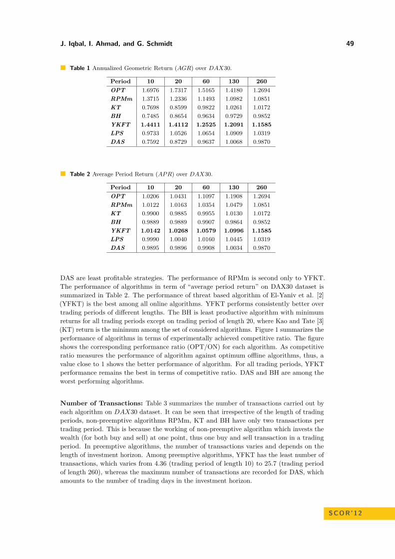
J. Iqbal, I. Ahmad, and G. Schmidt 49
Table 1 Annualized Geometric Return (AGR) over DAX30.
Period 10 20 60 130 260OPT 1.6976 1.7317 1.5165 1.4180 1.2694RPMm 1.3715 1.2336 1.1493 1.0982 1.0851KT 0.7698 0.8599 0.9822 1.0261 1.0172BH 0.7485 0.8654 0.9634 0.9729 0.9852YKFT 1.4411 1.4112 1.2525 1.2091 1.1585LPS 0.9733 1.0526 1.0654 1.0909 1.0319DAS 0.7592 0.8729 0.9637 1.0068 0.9870
Table 2 Average Period Return (AP R) over DAX30.
Period 10 20 60 130 260OPT 1.0206 1.0431 1.1097 1.1908 1.2694RPMm 1.0122 1.0163 1.0354 1.0479 1.0851KT 0.9900 0.9885 0.9955 1.0130 1.0172BH 0.9889 0.9889 0.9907 0.9864 0.9852YKFT 1.0142 1.0268 1.0579 1.0996 1.1585LPS 0.9990 1.0040 1.0160 1.0445 1.0319DAS 0.9895 0.9896 0.9908 1.0034 0.9870
DAS are least profitable strategies. The performance of RPMm is second only to YFKT.The performance of algorithms in term of “average period return” on DAX30 dataset issummarized in Table 2. The performance of threat based algorithm of El-Yaniv et al. [2](YFKT) is the best among all online algorithms. YFKT performs consistently better overtrading periods of different lengths. The BH is least productive algorithm with minimumreturns for all trading periods except on trading period of length 20, where Kao and Tate [3](KT) return is the minimum among the set of considered algorithms. Figure 1 summarizes theperformance of algorithms in terms of experimentally achieved competitive ratio. The figureshows the corresponding performance ratio (OPT/ON) for each algorithm. As competitiveratio measures the performance of algorithm against optimum offline algorithms, thus, avalue close to 1 shows the better performance of algorithm. For all trading periods, YFKTperformance remains the best in terms of competitive ratio. DAS and BH are among theworst performing algorithms.
Number of Transactions: Table 3 summarizes the number of transactions carried out byeach algorithm on DAX30 dataset. It can be seen that irrespective of the length of tradingperiods, non-preemptive algorithms RPMm, KT and BH have only two transactions pertrading period. This is because the working of non-preemptive algorithm which invests thewealth (for both buy and sell) at one point, thus one buy and sell transaction in a tradingperiod. In preemptive algorithms, the number of transactions varies and depends on thelength of investment horizon. Among preemptive algorithms, YFKT has the least number oftransactions, which varies from 4.36 (trading period of length 10) to 25.7 (trading periodof length 260), whereas the maximum number of transactions are recorded for DAS, whichamounts to the number of trading days in the investment horizon.
SCOR’12
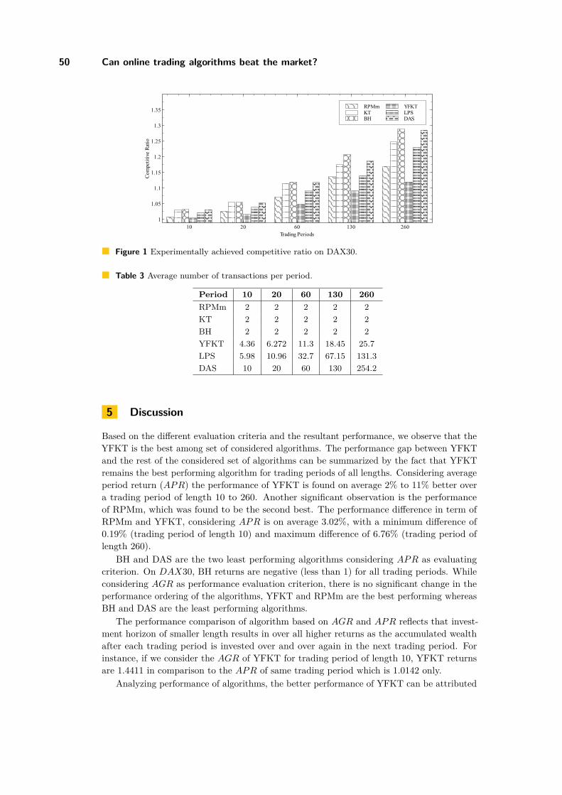
50 Can online trading algorithms beat the market?
RPMmKTBH
YFKTLPSDAS
Com
petit
ive
Ratio
1
1.05
1.1
1.15
1.2
1.25
1.3
1.35
Trading Periods10 20 60 130 260
Figure 1 Experimentally achieved competitive ratio on DAX30.
Table 3 Average number of transactions per period.
Period 10 20 60 130 260RPMm 2 2 2 2 2KT 2 2 2 2 2BH 2 2 2 2 2YFKT 4.36 6.272 11.3 18.45 25.7LPS 5.98 10.96 32.7 67.15 131.3DAS 10 20 60 130 254.2
5 Discussion
Based on the different evaluation criteria and the resultant performance, we observe that theYFKT is the best among set of considered algorithms. The performance gap between YFKTand the rest of the considered set of algorithms can be summarized by the fact that YFKTremains the best performing algorithm for trading periods of all lengths. Considering averageperiod return (APR) the performance of YFKT is found on average 2% to 11% better overa trading period of length 10 to 260. Another significant observation is the performanceof RPMm, which was found to be the second best. The performance difference in term ofRPMm and YFKT, considering APR is on average 3.02%, with a minimum difference of0.19% (trading period of length 10) and maximum difference of 6.76% (trading period oflength 260).
BH and DAS are the two least performing algorithms considering APR as evaluatingcriterion. On DAX30, BH returns are negative (less than 1) for all trading periods. Whileconsidering AGR as performance evaluation criterion, there is no significant change in theperformance ordering of the algorithms, YFKT and RPMm are the best performing whereasBH and DAS are the least performing algorithms.
The performance comparison of algorithm based on AGR and APR reflects that invest-ment horizon of smaller length results in over all higher returns as the accumulated wealthafter each trading period is invested over and over again in the next trading period. Forinstance, if we consider the AGR of YFKT for trading period of length 10, YFKT returnsare 1.4411 in comparison to the APR of same trading period which is 1.0142 only.
Analyzing performance of algorithms, the better performance of YFKT can be attributed
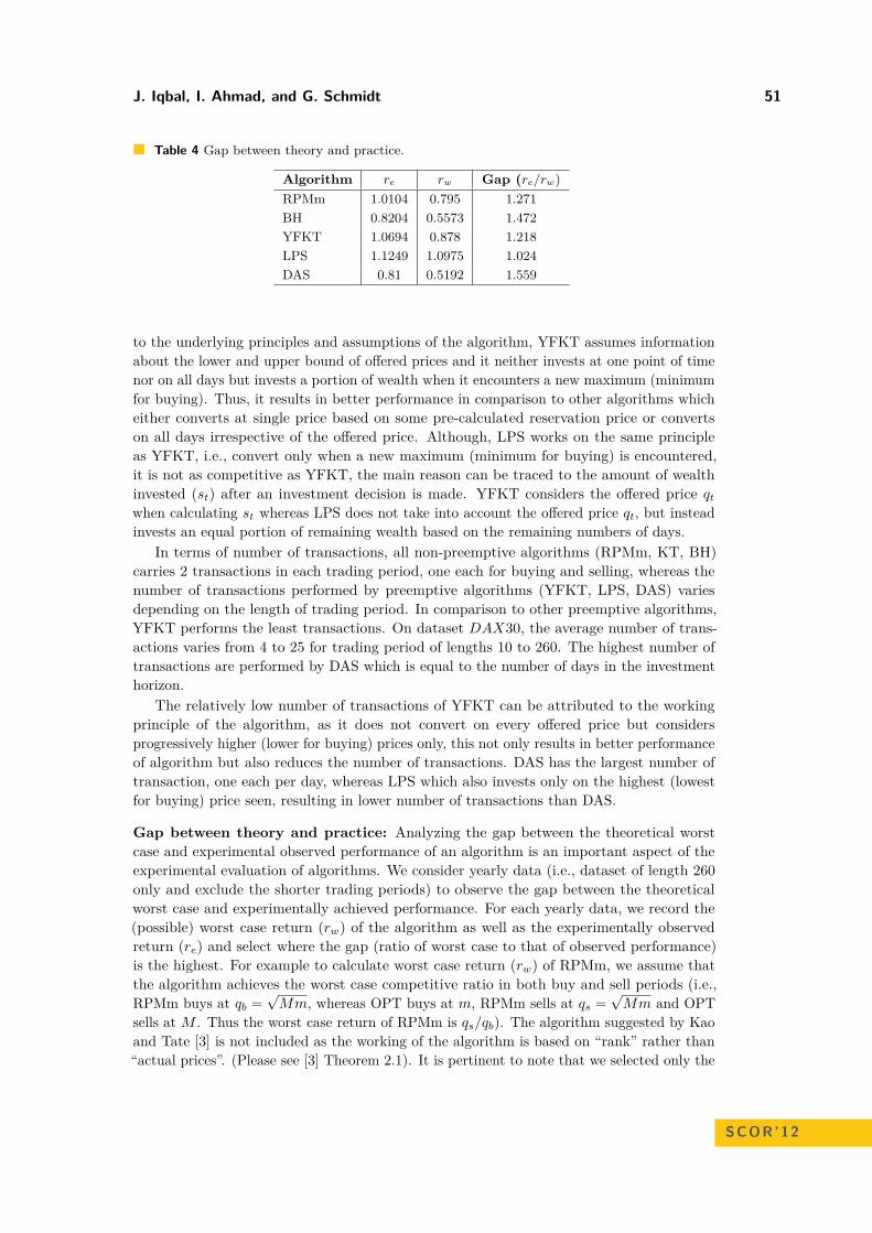
J. Iqbal, I. Ahmad, and G. Schmidt 51
Table 4 Gap between theory and practice.
Algorithm re rw Gap (re/rw)RPMm 1.0104 0.795 1.271BH 0.8204 0.5573 1.472YFKT 1.0694 0.878 1.218LPS 1.1249 1.0975 1.024DAS 0.81 0.5192 1.559
to the underlying principles and assumptions of the algorithm, YFKT assumes informationabout the lower and upper bound of offered prices and it neither invests at one point of timenor on all days but invests a portion of wealth when it encounters a new maximum (minimumfor buying). Thus, it results in better performance in comparison to other algorithms whicheither converts at single price based on some pre-calculated reservation price or convertson all days irrespective of the offered price. Although, LPS works on the same principleas YFKT, i.e., convert only when a new maximum (minimum for buying) is encountered,it is not as competitive as YFKT, the main reason can be traced to the amount of wealthinvested (st) after an investment decision is made. YFKT considers the offered price qt
when calculating st whereas LPS does not take into account the offered price qt, but insteadinvests an equal portion of remaining wealth based on the remaining numbers of days.
In terms of number of transactions, all non-preemptive algorithms (RPMm, KT, BH)carries 2 transactions in each trading period, one each for buying and selling, whereas thenumber of transactions performed by preemptive algorithms (YFKT, LPS, DAS) variesdepending on the length of trading period. In comparison to other preemptive algorithms,YFKT performs the least transactions. On dataset DAX30, the average number of trans-actions varies from 4 to 25 for trading period of lengths 10 to 260. The highest number oftransactions are performed by DAS which is equal to the number of days in the investmenthorizon.
The relatively low number of transactions of YFKT can be attributed to the workingprinciple of the algorithm, as it does not convert on every offered price but considersprogressively higher (lower for buying) prices only, this not only results in better performanceof algorithm but also reduces the number of transactions. DAS has the largest number oftransaction, one each per day, whereas LPS which also invests only on the highest (lowestfor buying) price seen, resulting in lower number of transactions than DAS.
Gap between theory and practice: Analyzing the gap between the theoretical worstcase and experimental observed performance of an algorithm is an important aspect of theexperimental evaluation of algorithms. We consider yearly data (i.e., dataset of length 260only and exclude the shorter trading periods) to observe the gap between the theoreticalworst case and experimentally achieved performance. For each yearly data, we record the(possible) worst case return (rw) of the algorithm as well as the experimentally observedreturn (re) and select where the gap (ratio of worst case to that of observed performance)is the highest. For example to calculate worst case return (rw) of RPMm, we assume thatthe algorithm achieves the worst case competitive ratio in both buy and sell periods (i.e.,RPMm buys at qb =
√Mm, whereas OPT buys at m, RPMm sells at qs =
√Mm and OPT
sells at M . Thus the worst case return of RPMm is qs/qb). The algorithm suggested by Kaoand Tate [3] is not included as the working of the algorithm is based on “rank” rather than“actual prices”. (Please see [3] Theorem 2.1). It is pertinent to note that we selected only the
SCOR’12
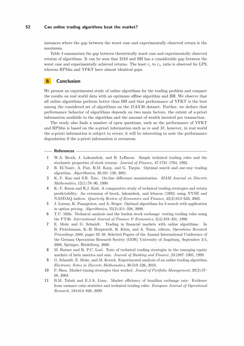
52 Can online trading algorithms beat the market?
instances where the gap between the worst case and experimentally observed return is themaximum.
Table 4 summarizes the gap between theoretically worst case and experimentally observedreturns of algorithms. It can be seen that DAS and BH has a considerable gap between theworst case and experimentally achieved returns. The least re to rw ratio is observed for LPS,whereas RPMm and YFKT have almost identical gaps.
6 Conclusion
We present an experimental study of online algorithms for the trading problem and comparethe results on real world data with an optimum offline algorithm and BH. We observe thatall online algorithms perform better than BH and that performance of YFKT is the bestamong the considered set of algorithms on the DAX30 dataset. Further, we deduce thatperformance behavior of algorithms depends on two main factors, the extent of a-prioriinformation available to the algorithm and the amount of wealth invested per transaction.
The study also finds a number of open questions, such as the performance of YFKTand RPMm is based on the a-priori information such as m and M , however, in real worldthe a-priori information is subject to errors, it will be interesting to note the performancedegradation if the a-priori information is erroneous.
References1 W.A. Brock, J. Lakonishok, and B. LeBaron. Simple technical trading rules and the
stochastic properties of stock returns. Journal of Finance, 47:1731–1764, 1992.2 R. El-Yaniv, A. Fiat, R.M. Karp, and G. Turpin. Optimal search and one-way trading
algorithm. Algorithmica, 30:101–139, 2001.3 K.-Y. Kao and S.R. Tate. On-line difference maximization. SIAM Journal on Discrete
Mathematics, 12(1):78–90, 1999.4 K.-Y. Kwon and R.J. Kish. A comparative study of technical trading strategies and return
predictability: An extension of brock, lakonishok, and lebaron (1992) using NYSE andNASDAQ indices. Quarterly Review of Economics and Finance, 42(3):613–633, 2002.
5 J. Lorenz, K. Panagiotou, and A. Steger. Optimal algorithms for k-search with applicationin option pricing. Algorithmica, 55(2):311–328, 2009.
6 T.C. Mills. Technical analysis and the london stock exchange: testing trading rules usingthe FT30. International Journal of Finance & Economics, 2(4):319–331, 1998.
7 E. Mohr and G. Schmidt. Trading in financial markets with online algorithms. InB. Fleischmann, K.-H. Borgwardt, R. Klein, and A. Tuma, editors, Operations ResearchProceedings 2008, pages 33–38. Selected Papers of the Annual International Conference ofthe German Operations Research Society (GOR) University of Augsburg, September 3-5,2008, Springer, Heidelberg, 2008.
8 M. Ratner and R. P.C. Leal. Tests of technical trading strategies in the emerging equitymarkets of latin america and asia. Journal of Banking and Finance, 23:1887–1905, 1999.
9 G. Schmidt, E. Mohr, and M. Kersch. Experimental analysis of an online trading algorithm.Electronic Notes in Discrete Mathematics, 36:519–526, 2010.
10 P. Shen. Market-timing strategies that worked. Jounal of Portfolio Management, 29(2):57–68, 2003.
11 B.M. Tabak and E.J.A. Lima. Market efficiency of brazilian exchange rate: Evidencefrom variance ratio statistics and technical trading rules. European Journal of OperationalResearch, 194:814–820, 2009.
An exact algorithm for the uncertain version ofparallel machines scheduling problem with thetotal completion time criterionMarcin Siepak1
1 Wroclaw University of Technology/Institute of InformaticsWybrzeze Wyspianskiego 27, 50-370 [email protected]
AbstractAn uncertain version of parallel and identical machines scheduling problem with total completiontime criterion is considered. It is assumed that the execution times of tasks are not knowna priori but they belong to the intervals of known bounds. The absolute regret based approachfor coping with such an uncertainty is applied. This problem is known to be NP-hard anda branch and bound algorithm (B&B) for finding the exact solution is developed. The results ofcomputational experiments show that for the tested instances of the uncertain problem — B&Bworks significantly faster than the exact procedure based on enumeration of all the solutions.The algorithm proposed has application for further research of quality evaluation for heuristicand approximate solution approaches for the considered problem (in order to check how far fromthe optimality are solutions generated by them) and also in the cases where the requirement isto obtain the exact solutions for the uncertain problem.
1998 ACM Subject Classification I.2.8 Problem Solving, Control Methods, and Search
Keywords and phrases Task scheduling, Interval uncertainty, Minmax regret, Branch and Bound
Digital Object Identifier 10.4230/OASIcs.SCOR.2012.53
1 Introduction
P‖∑Ci is classical scheduling problem polynomially solvable ([3], [5]). It consists in
scheduling the set of I tasks on the set of J parallel and identical machines. The executiontimes pi, i = 1, . . . , I are given. The optimal schedule minimizes the total flow time
∑i Ci,
i.e. the sum of tasks completion times where Ci is the completion time of the ith task. Sucha schedule, at each point of time maximizes the number of tasks already processed, by firstscheduling those which execution time is the shortest. In order to solve the problem, itis required to assign tasks to the machines and also fix the tasks execution order on eachmachine.
In this paper we consider the uncertain version of P‖∑Ci where the execution times
pi are imprecise. The uncertainty is modelled by the concept of a scenario which is anassignment of possible values into the imprecise parameters of the problem [1]. The set of allpossible scenarios can be described in two ways — in the discrete scenario case, the possiblevalues of uncertain parameters are presented explicitely and in the interval scenario casethey can take any value between a lower and upper bound. Hereinafter we consider theinterval case where we assume that for each of tasks only the borders of the intervals p
iand
pi are given where pi6 pi and pi ∈
[p
i, pi
]. Such a way of uncertainty description is useful
in the cases where no historical data is available regarding the imprecise parameters, which© Marcin Siepak;licensed under Creative Commons License NC-ND
3rd Student Conference on Operational Research (SCOR 2012).Editors: Stefan Ravizza and Penny Holborn; pp. 53–63
OpenAccess Series in InformaticsSchloss Dagstuhl – Leibniz-Zentrum für Informatik, Dagstuhl Publishing, Germany
54 An exact algorithm for the uncertain version of parallel machines scheduling problem
would be required in order to obtain the probability distribution and apply the stochasticapproach and also when there is lack of experts opinions which would be a source of otherrepresentations of uncertain execution times, e.g. in the form of a membership function forthe fuzzy approach.
To solve the nondeterministic case, one can assume the specific values of uncertainparameters and use the deterministic approach. The quality of such a solution however, maybe poor because assumed values may differ greatly from the actual ones. For the considerednondeterministic problem, we use therefore the approach based on the absolute opportunityloss (regret) introduced by Savage in [12] and the concept of minmax regret ([2], [9]) whichrequires finding a feasible solution that is ε-optimal for any possible scenario with ε as smallas possible [1].
Minmax regret versions of many classical optimization problems were studied in [1] and[6]. Newer results were recently obtained in [2], [7], [13], [14].
The paper is organised as follows. The deterministic and uncertain versions of theconsidered problem are formulated in Section 2. The solution algorithm proposed is presentedin Section 3. Section 4 is devoted to description of the computational experiments and theirresults. In Section 5, the conclusions are presented.
2 Problem formulation
2.1 Deterministic caseLet us introduce the following notation:I = {1, 2, . . . , I} — set of tasks,J = {1, 2, . . . , J} — set of machines,p = [pi]i=1,...,I — vector of task execution times.Moreover, let x = [xikj ]i=1,...,I;k=1,...,I;j=1,...,J be the matrix of binary optimization variableswhere xikj = 1 if the ith task is scheduled as the kth to the last task on machine j, and 0otherwise. Each machine has therefore I virtual positions, where tasks can be assigned toand parameter k specifies index of the position to the last where a task can be performed.
The objective function is expressed as the sum of tasks completion times [11]:
F (p, x) =I∑
i=1pi
J∑j=1
I∑k=1
kxikj . (1)
The following constraints are imposed on optimization variables xikj . Each task isperformed on exactly one position of exactly one machine:
J∑j=1
I∑k=1
xikj = 1; i = 1, . . . , I. (2)
Maximally one task can be performed on each position of each machine:
I∑i=1
xikj 6 1; j = 1, . . . , J ; k = 1, . . . , I. (3)
The elements of matrix x are binary optimization variables:
xikj ∈ {0, 1} ; i = 1, . . . , I; j = 1, . . . , J ; k = 1, . . . , I. (4)
M. Siepak 55
Therefore, formulation of deterministic version of P‖∑Ci is as follows
F′(p) , F (p, x
′) = min
xF (p, x) =
I∑i=1
pi
J∑j=1
I∑k=1
kx′
ikj (5)
subject to (2), (3) and (4).
2.2 Uncertain caseFor the uncertain case, we assume that the exact value of execution time pi is not given, andthis parameter belongs to the interval
[p
i, pi
]where p
iand pi are known. It means that we
consider uncertain parameters pi described by a set of their possible values in the form ofintervals. No other characteristics of such an uncertainty are assumed or used. A particularvector p expresses fixed configuration of the execution times and is called a scenario. A set
P =[p1, p1
]× . . .×
[p
I, pI
](6)
of all scenarios is characterized by the Cartesian product of all the intervals. A scenariowhere completion times of all tasks are equal borders of the corresponding intervals p
ior pi
is called an extreme scenario.In order to measure solution quality for the nondeterministic problem, we apply absolute
regret as introduced by Savage in [12]. It expresses the difference between value of the totalflow time criterion for given solution x and specified scenario p as well as optimal value ofthe total flow time criterion for p:
F (p, x)− F′(p). (7)
To find solution of the problem, the robust approach ([1], [9]) is applied. For specifiedsolution x the uncertain parameters are determined by obtaining so called worst case scenariodenoted by px, i.e. the one which maximizes absolute regret:
z(x) = maxp∈P
[F (p, x)− F
′(p)]. (8)
The optimal solution x∗ for the uncertain version of P‖∑Ci minimizes (8), i.e. z∗ , z(x∗) =
minx z(x) subject to (2), (3) and (4).
3 Solution algorithm
3.1 Deterministic caseThe deterministic version of P‖
∑Ci is polynomially solvable and the optimal solution can
be obtained using SPT (Shortest Processing Time) rule [11]. This procedure sorts all thetasks in nonincreasing order according to their execution times. They are assigned iterativelythen, i.e. the i’th task is assigned into the first available position to the last (i.e. not occupiedposition, such that the value of parameter k is the smallest) on the n’th machine, where
n ={J, when (i mod J) = 0(i mod J), otherwise. (9)
SCOR’12
56 An exact algorithm for the uncertain version of parallel machines scheduling problem
3.2 Uncertain caseThe uncertain version of P‖
∑Ci is NP-hard which results directly from NP-hardness of the
nondeterministic version of a single machine scheduling problem, i.e. 1‖∑Ci [10].
Let us denote by Pe the set of extreme scenarios, i.e.
Pe ={p1, p1
}× . . .×
{p
I, pI
}. (10)
and by px the worst-case scenario for solution x.
I Lemma 1. px ∈ Pe for any feasible solution x.
Proof. It is easy to see, that for two feasible solutions x1 and x2 the following equality holds:
F (p, x1)− F (p, x2) =I∑
i=1pi
J∑j=1
I∑k=1
kx1ikj −
I∑i=1
pi
J∑j=1
I∑k=1
kx2ikj
=I∑
i=1pi
J∑j=1
(kx1
ij − kx2
ij
)(11)
where for any feasible solution xs:
kxs
ij ={k ∈ {1, . . . , J} if ∃k : xs
ikj = 10 if ∀k = 1, . . . , I xs
ikj = 0. (12)
As a result of (11) we get:
F (p, x)− F′(p) =
I∑i=1
pi
J∑j=1
(kx
ij − kx′
ij
). (13)
Now, in order to maximize (13) and obtain the worst-case scenario, it is enough to assume:
pi ={
pi, when ∃jx, jx′ ∈ {1, . . . , J} : kxijx
> 0 ∧ kx′
ijx
′ > 0 ∧ kxijx
> kx′
ijx
′
pi, otherwise.
(14)
From (14) it results immediately, that ∀i either pi ∈ px or pi∈ px and consequently px ⊂ Pe
for each solution x. J
3.3 Branch and bound algorithmAs a consequence of NP-hardness of the uncertain version of P‖
∑Ci, we apply Branch and
Bound procedure (B&B) [4] which allows to obtain the exact solution for small instances ofthe problem faster than the algorithm based on a simple enumeration (denoted as EXCT).B&B can therefore be applied to larger instances of the uncertain problem, which solvingusing EXCT procedure would take unacceptably long time in the real life systems. Accordingto B&B, the main complex and hard to solve input problem denoted as OPT is decomposedinto a finite number of subproblems OPT1, OPT2, ..., OPTq where the corresponding subsetsof feasible solutions Q1, . . . , Qq, fulfill conditions Ql∩Qm = ∅ for l 6= m and Q1∪. . .∪Qq = Q,where Q is a set of feasible solutions for OPT . The process of decomposition can representedin a form of partition tree where the root corresponds to the input problem OPT andthe nodes represent individual subproblems. For each subproblem, until it is fulfilled bymaximally one solution — a further decomposition can be performed.
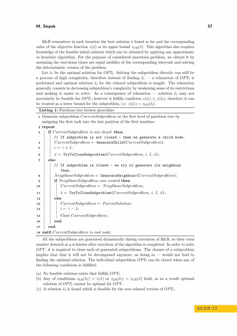
M. Siepak 57
B&B remembers in each iteration the best solution x found so far and the correspondingvalue of the objective function z(x) or its upper bound zUB(x). This algorithm also requiresknowledge of the feasible initial solution which can be obtained by applying any approximateor heuristic algorithm. For the purpose of considered uncertain problem, we obtain it byassuming the execution times are equal middles of the corresponding intervals and solvingthe deterministic version of the problem.
Let xl be the optimal solution for OPTl. Solving the subproblem directly can still bea process of high complexity, therefore instead of finding xl — a relaxation of OPTl isperformed and optimal solution xl for the relaxed subproblem is sought. The relaxationgenerally consists in decreasing subproblem’s complexity by weakening some of its restrictionsand making it easier to solve. As a consequence of relaxation — solution xl may notnecessirely be feasible for OPTl, however it fulfills condition z(xl) ≤ z(xl), therefore it canbe treated as a lower bound for the subproblem, i.e. z(xl) = zLB(xl).
Listing 1: Partition tree browse procedure1 Generate subproblem CurrentSubproblem at the first level of partition tree byassigning the first task into the last position of the first machine;
2 repeat3 if CurrentSubproblem is not closed then
// If subproblem is not closed - then we generate a child node.4 CurrentSubproblem ← GenerateChild(CurrentSubproblem);5 i ← i + 1;
6 x ← TryToCloseSubproblem(CurrentSubproblem, i, I, x);7 else
// If subproblem is closed - we try to generate its neighbourthen.
8 NeighbourSubproblem ← GenerateNeighbour(CurrentSubproblem);9 if NeighbourSubproblem was created then
10 CurrentSubproblem ← NeighbourSubproblem;
11 x ← TryToCloseSubproblem(CurrentSubproblem, i, I, x);12 else13 CurrentSubproblem ← ParentSolution;14 i ← i − 1;
15 Close CurrentSubproblem ;16 end17 end18 until CurrentSubproblem is root node;
All the subproblems are generated dynamically during execution of B&B, so their totalnumber denoted as q is known after execution of the algorithm is completed. In order to solveOPT , it is required to close each of generated subproblems. The closure of a subproblemimplies that that it will not be decomposed anymore, as doing so — would not lead tofinding the optimal solution. The individual subproblem OPTl can be closed when any ofthe following conditions is fulfilled:
(a) No feasible solution exists that fulfills OPTl.(b) Any of conditions zLB(xl) > z(x) or zLB(xl) > zUB(x) hold, so as a result optimal
solution of OPTl cannot be optimal for OPT .(c) A solution xl is found which is feasible for the non relaxed version of OPTl.
SCOR’12
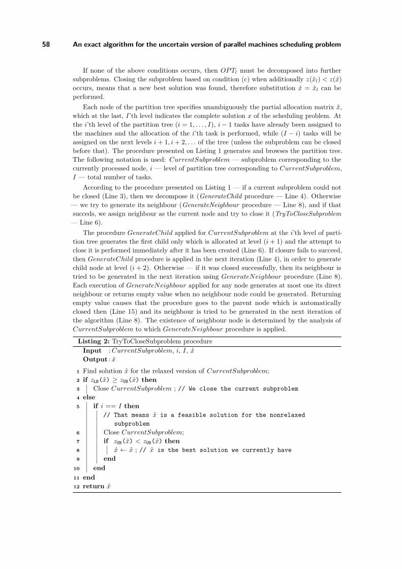
58 An exact algorithm for the uncertain version of parallel machines scheduling problem
If none of the above conditions occurs, then OPTl must be decomposed into furthersubproblems. Closing the subproblem based on condition (c) when additionally z(xl) < z(x)occurs, means that a new best solution was found, therefore substitution x = xl can beperformed.
Each node of the partition tree specifies unambiguously the partial allocation matrix x,which at the last, I’th level indicates the complete solution x of the scheduling problem. Atthe i’th level of the partition tree (i = 1, . . . , I), i− 1 tasks have already been assigned tothe machines and the allocation of the i’th task is performed, while (I − i) tasks will beassigned on the next levels i+ 1, i+ 2, . . . of the tree (unless the subproblem can be closedbefore that). The procedure presented on Listing 1 generates and browses the partition tree.The following notation is used: CurrentSubproblem — subproblem corresponding to thecurrently processed node, i — level of partition tree corresponding to CurrentSubproblem,I — total number of tasks.
According to the procedure presented on Listing 1 — if a current subproblem could notbe closed (Line 3), then we decompose it (GenerateChild procedure — Line 4). Otherwise— we try to generate its neighbour (GenerateNeighbour procedure — Line 8), and if thatsucceds, we assign neighbour as the current node and try to close it (TryToCloseSubproblem— Line 6).
The procedure GenerateChild applied for CurrentSubproblem at the i’th level of parti-tion tree generates the first child only which is allocated at level (i+ 1) and the attempt toclose it is performed immediately after it has been created (Line 6). If closure fails to succeed,then GenerateChild procedure is applied in the next iteration (Line 4), in order to generatechild node at level (i+ 2). Otherwise — if it was closed successfully, then its neighbour istried to be generated in the next iteration using GenerateNeighbour procedure (Line 8).Each execution of GenerateNeighbour applied for any node generates at most one its directneighbour or returns empty value when no neighbour node could be generated. Returningempty value causes that the procedure goes to the parent node which is automaticallyclosed then (Line 15) and its neighbour is tried to be generated in the next iteration ofthe algorithm (Line 8). The existence of neighbour node is determined by the analysis ofCurrentSubproblem to which GenerateNeighbour procedure is applied.
Listing 2: TryToCloseSubproblem procedureInput :CurrentSubproblem, i, I, xOutput : x
1 Find solution x for the relaxed version of CurrentSubproblem;2 if zLB(x) ≥ zUB(x) then3 Close CurrentSubproblem ; // We close the current subproblem4 else5 if i == I then
// That means x is a feasible solution for the nonrelaxedsubproblem
6 Close CurrentSubproblem;7 if zUB(x) < zUB(x) then8 x ← x ; // x is the best solution we currently have9 end
10 end11 end12 return x
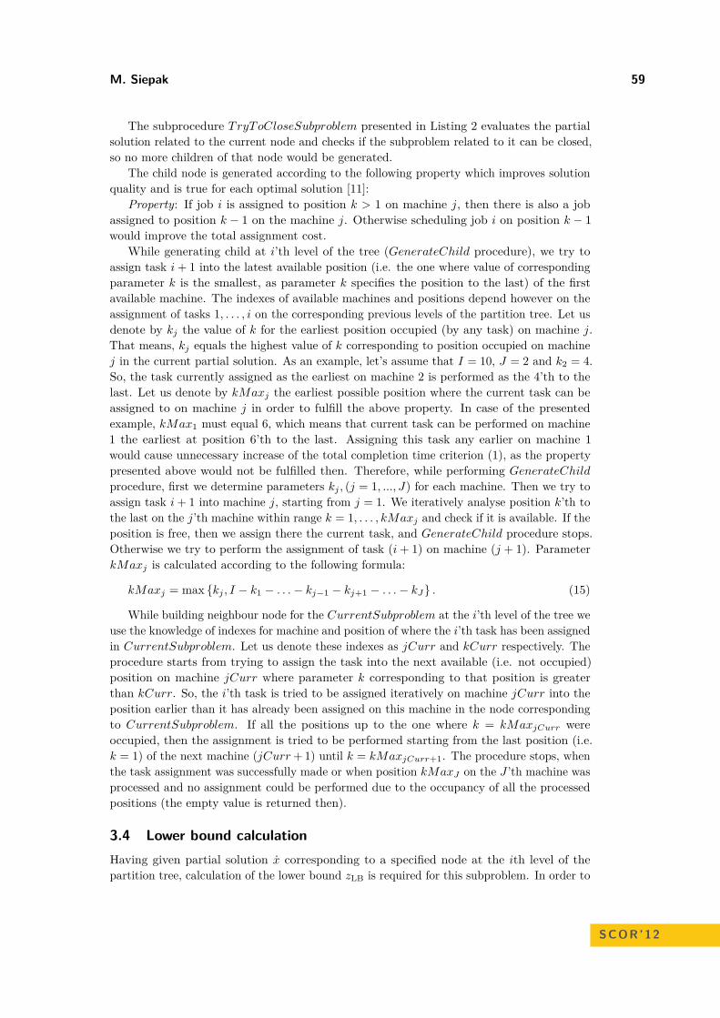
M. Siepak 59
The subprocedure TryToCloseSubproblem presented in Listing 2 evaluates the partialsolution related to the current node and checks if the subproblem related to it can be closed,so no more children of that node would be generated.
The child node is generated according to the following property which improves solutionquality and is true for each optimal solution [11]:
Property: If job i is assigned to position k > 1 on machine j, then there is also a jobassigned to position k − 1 on the machine j. Otherwise scheduling job i on position k − 1would improve the total assignment cost.
While generating child at i’th level of the tree (GenerateChild procedure), we try toassign task i+ 1 into the latest available position (i.e. the one where value of correspondingparameter k is the smallest, as parameter k specifies the position to the last) of the firstavailable machine. The indexes of available machines and positions depend however on theassignment of tasks 1, . . . , i on the corresponding previous levels of the partition tree. Let usdenote by kj the value of k for the earliest position occupied (by any task) on machine j.That means, kj equals the highest value of k corresponding to position occupied on machinej in the current partial solution. As an example, let’s assume that I = 10, J = 2 and k2 = 4.So, the task currently assigned as the earliest on machine 2 is performed as the 4’th to thelast. Let us denote by kMaxj the earliest possible position where the current task can beassigned to on machine j in order to fulfill the above property. In case of the presentedexample, kMax1 must equal 6, which means that current task can be performed on machine1 the earliest at position 6’th to the last. Assigning this task any earlier on machine 1would cause unnecessary increase of the total completion time criterion (1), as the propertypresented above would not be fulfilled then. Therefore, while performing GenerateChildprocedure, first we determine parameters kj , (j = 1, ..., J) for each machine. Then we try toassign task i+ 1 into machine j, starting from j = 1. We iteratively analyse position k’th tothe last on the j’th machine within range k = 1, . . . , kMaxj and check if it is available. If theposition is free, then we assign there the current task, and GenerateChild procedure stops.Otherwise we try to perform the assignment of task (i+ 1) on machine (j + 1). ParameterkMaxj is calculated according to the following formula:
kMaxj = max {kj , I − k1 − . . .− kj−1 − kj+1 − . . .− kJ} . (15)
While building neighbour node for the CurrentSubproblem at the i’th level of the tree weuse the knowledge of indexes for machine and position of where the i’th task has been assignedin CurrentSubproblem. Let us denote these indexes as jCurr and kCurr respectively. Theprocedure starts from trying to assign the task into the next available (i.e. not occupied)position on machine jCurr where parameter k corresponding to that position is greaterthan kCurr. So, the i’th task is tried to be assigned iteratively on machine jCurr into theposition earlier than it has already been assigned on this machine in the node correspondingto CurrentSubproblem. If all the positions up to the one where k = kMaxjCurr wereoccupied, then the assignment is tried to be performed starting from the last position (i.e.k = 1) of the next machine (jCurr+ 1) until k = kMaxjCurr+1. The procedure stops, whenthe task assignment was successfully made or when position kMaxJ on the J ’th machine wasprocessed and no assignment could be performed due to the occupancy of all the processedpositions (the empty value is returned then).
3.4 Lower bound calculationHaving given partial solution x corresponding to a specified node at the ith level of thepartition tree, calculation of the lower bound zLB is required for this subproblem. In order to
SCOR’12
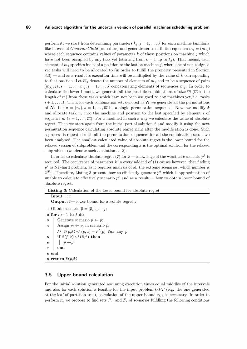
60 An exact algorithm for the uncertain version of parallel machines scheduling problem
perform it, we start from determining parameters kj , j = 1, . . . , J for each machine (similarlylike in case of GenerateChild procedure) and generate series of finite sequences mj = (mjs
)where each sequence contains values of parameter k of those positions on machine j whichhave not been occupied by any task yet (starting from k = 1 up to kj). That means, eachelement of mj specifies index of a position to the last on machine j, where one of non assignedyet tasks will need to be allocated to (in order to fulfill the property presented in Section3.3) — and as a result its execution time will be multiplied by the value of k correspondingto that position. Let mj denote the number of elements of mj and m be a sequence of pairs(mjs
, j) , s = 1, . . . ,mj ; j = 1, . . . , J concatenating elements of sequences mj . In order tocalculate the lower bound, we generate all the possible combinations of size m (m is thelength of m) from these tasks which have not been assigned to any machines yet, i.e. tasksi+ 1, . . . , I. Then, for each combination set, denoted as N we generate all the permutationsof N . Let n = (ns), s = 1, . . . ,m be a single permutation sequence. Now, we modify xand allocate task ns into the machine and position to the last specified by element s ofsequence m (s = 1, . . . ,m). For x modified in such a way we calculate the value of absoluteregret. Then we start again from the initial partial solution x and modify it using the nextpermutation sequence calculating absolute regret right after the modification is done. Sucha process is repeated until all the permutation sequences for all the combination sets havebeen analysed. The smallest calculated value of absolute regret is the lower bound for therelaxed version of subproblem and the corresponding x is the optimal solution for the relaxedsubproblem (we denote such a solution as x).
In order to calculate absolute regret (7) for x— knowledge of the worst case scenario px isrequired. The occurrence of parameter k in every addend of (1) causes however, that findingpx is NP-hard problem, as it requires analysis of all the extreme scenarios, which number is2|Pe|. Therefore, Listing 3 presents how to efficiently generate px which is approximation ofunable to calculate effectively scenario px and as a result — how to obtain lower bound ofabsolute regret.
Listing 3: Calculation of the lower bound for absolute regretInput : xOutput : z— lower bound for absolute regret z
1 Obtain scenario p = [pi]i=1...,I ;2 for i← 1 to I do3 Generate scenario p ← p;4 Assign pi ← p
iin scenario p;
// z(p,x)=F (p, x)− F ′(p) for any p
5 if z(p,x)>z(p,x) then6 p ←p;7 end8 end9 return z(p,x)
3.5 Upper bound calculation
For the initial solution generated assuming execution times equal middles of the intervalsand also for each solution x feasible for the input problem OPT (e.g. the one generatedat the leaf of partition tree), calculation of the upper bound zUB is necessary. In order toperform it, we propose to find sets Pm and Ps of scenarios fulfilling the following conditions
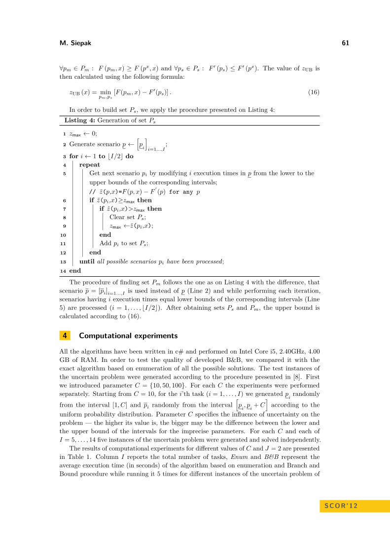
M. Siepak 61
∀pm ∈ Pm : F (pm, x) ≥ F (px, x) and ∀ps ∈ Ps : F ′ (ps) ≤ F ′ (px). The value of zUB isthen calculated using the following formula:
zUB (x) = minpm,ps
[F (pm, x)− F ′(ps)] . (16)
In order to build set Ps, we apply the procedure presented on Listing 4:Listing 4: Generation of set Ps
1 zmax ← 0;2 Generate scenario p ←
[p
i
]i=1...,I
;
3 for i← 1 to bI/2c do4 repeat5 Get next scenario pi by modifying i execution times in p from the lower to the
upper bounds of the corresponding intervals;// z(p,x)=F (p, x)− F ′(p) for any p
6 if z(pi,x)≥zmax then7 if z(pi,x)>zmax then8 Clear set Ps;9 zmax ←z(pi,x);
10 end11 Add pi to set Ps;12 end13 until all possible scenarios pi have been processed;14 end
The procedure of finding set Pm follows the one as on Listing 4 with the difference, thatscenario p = [pi]i=1...,I is used instead of p (Line 2) and while performing each iteration,scenarios having i execution times equal lower bounds of the corresponding intervals (Line5) are processed (i = 1, . . . , bI/2c). After obtaining sets Ps and Pm, the upper bound iscalculated according to (16).
4 Computational experiments
All the algorithms have been written in c# and performed on Intel Core i5, 2.40GHz, 4.00GB of RAM. In order to test the quality of developed B&B, we compared it with theexact algorithm based on enumeration of all the possible solutions. The test instances ofthe uncertain problem were generated according to the procedure presented in [8]. Firstwe introduced parameter C = {10, 50, 100}. For each C the experiments were performedseparately. Starting from C = 10, for the i’th task (i = 1, . . . , I) we generated p
irandomly
from the interval [1, C] and pi randomly from the interval[p
i, p
i+ C
]according to the
uniform probability distribution. Parameter C specifies the influence of uncertainty on theproblem — the higher its value is, the bigger may be the difference between the lower andthe upper bound of the intervals for the imprecise parameters. For each C and each ofI = 5, . . . , 14 five instances of the uncertain problem were generated and solved independently.
The results of computational experiments for different values of C and J = 2 are presentedin Table 1. Column I reports the total number of tasks, Enum and B&B represent theaverage execution time (in seconds) of the algorithm based on enumeration and Branch andBound procedure while running it 5 times for different instances of the uncertain problem of
SCOR’12
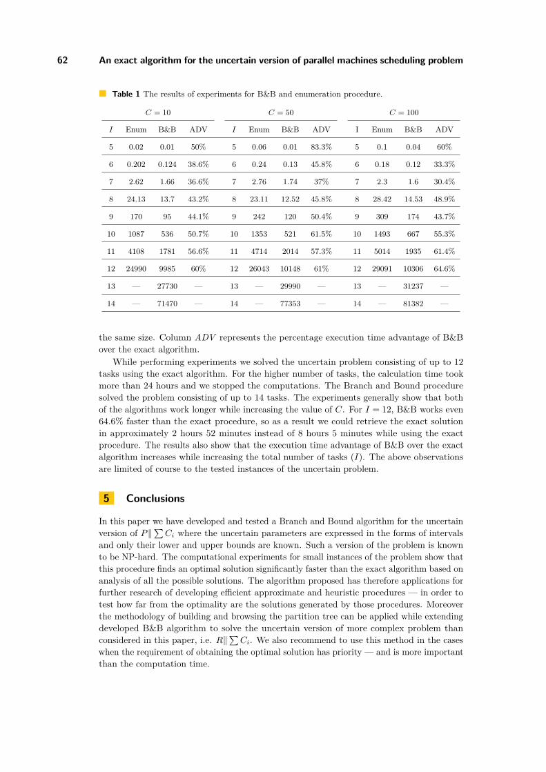
62 An exact algorithm for the uncertain version of parallel machines scheduling problem
Table 1 The results of experiments for B&B and enumeration procedure.
C = 10 C = 50 C = 100
I Enum B&B ADV I Enum B&B ADV I Enum B&B ADV
5 0.02 0.01 50% 5 0.06 0.01 83.3% 5 0.1 0.04 60%
6 0.202 0.124 38.6% 6 0.24 0.13 45.8% 6 0.18 0.12 33.3%
7 2.62 1.66 36.6% 7 2.76 1.74 37% 7 2.3 1.6 30.4%
8 24.13 13.7 43.2% 8 23.11 12.52 45.8% 8 28.42 14.53 48.9%
9 170 95 44.1% 9 242 120 50.4% 9 309 174 43.7%
10 1087 536 50.7% 10 1353 521 61.5% 10 1493 667 55.3%
11 4108 1781 56.6% 11 4714 2014 57.3% 11 5014 1935 61.4%
12 24990 9985 60% 12 26043 10148 61% 12 29091 10306 64.6%
13 — 27730 — 13 — 29990 — 13 — 31237 —
14 — 71470 — 14 — 77353 — 14 — 81382 —
the same size. Column ADV represents the percentage execution time advantage of B&Bover the exact algorithm.
While performing experiments we solved the uncertain problem consisting of up to 12tasks using the exact algorithm. For the higher number of tasks, the calculation time tookmore than 24 hours and we stopped the computations. The Branch and Bound proceduresolved the problem consisting of up to 14 tasks. The experiments generally show that bothof the algorithms work longer while increasing the value of C. For I = 12, B&B works even64.6% faster than the exact procedure, so as a result we could retrieve the exact solutionin approximately 2 hours 52 minutes instead of 8 hours 5 minutes while using the exactprocedure. The results also show that the execution time advantage of B&B over the exactalgorithm increases while increasing the total number of tasks (I). The above observationsare limited of course to the tested instances of the uncertain problem.
5 Conclusions
In this paper we have developed and tested a Branch and Bound algorithm for the uncertainversion of P‖
∑Ci where the uncertain parameters are expressed in the forms of intervals
and only their lower and upper bounds are known. Such a version of the problem is knownto be NP-hard. The computational experiments for small instances of the problem show thatthis procedure finds an optimal solution significantly faster than the exact algorithm based onanalysis of all the possible solutions. The algorithm proposed has therefore applications forfurther research of developing efficient approximate and heuristic procedures — in order totest how far from the optimality are the solutions generated by those procedures. Moreoverthe methodology of building and browsing the partition tree can be applied while extendingdeveloped B&B algorithm to solve the uncertain version of more complex problem thanconsidered in this paper, i.e. R‖
∑Ci. We also recommend to use this method in the cases
when the requirement of obtaining the optimal solution has priority — and is more importantthan the computation time.
M. Siepak 63
References1 H. Aissi, C. Bazgan, and D. Vanderpooten. Minmax and minmax regret versions of com-
binatorial optimization problems: A survey. European Journal of Operational Research,197:427–438, 2009.
2 I. Averbakh and J. Pereira. Exact and heuristic algorithms for the interval data robustassignment problem. Computers & Operations Research, 38:1153–1163, 2011.
3 J. Bruno, E. G. Coffman, Jr., and R. Sethi. Scheduling independent tasks to reduce meanfinishing time. Communications of the ACM, 17:382–387, 1974.
4 M. J. Brusco and S. Stahl. Branch-and-bound applications in combinatorial data analysis.Springer, 2005.
5 W. A. Horn. Minimizing average flow time with parallel machines. Operations Research,21:846–847, 1973.
6 A. Kasperski. Discrete Optimization with Interval Data: Minmax Regret and Fuzzy Ap-proach (Studies in Fuzziness and Soft Computing). Springer, Berlin, Heidelberg, New York,2008.
7 A. Kasperski, A. Kurpisz, and P. Zielinski. Approximating a two-machine flow shop schedul-ing under discrete scenario uncertainty. European Journal of Operational Research, 217:36–43, 2012.
8 A. Kasperski and P. Zielinski. Minimizing maximal regret in linear assignment problemswith interval data. Technical Report 07, Raport Serii PREPRINTY, Wroclaw, 2004.
9 P. Kouvelis and G. Yu. Robust Discrete Optimization and Its Applications. Kluwer Aca-demic Publishers, Dortrecht, Boston, London, 1997.
10 V. Lebedev and I. Averbakh. Complexity of minimizing the total flow time with intervaldata and minmax regret criterion. Discrete Applied Mathematics, 154:2167–2177, 2006.
11 M. L. Pinedo. Scheduling - Theory, Algorithms and Systems. Springer, New York, 2008.12 L. J. Savage. The theory of statistical decision. Journal of the American Statistical Asso-
ciation, 46:55–67, 1951.13 M. Siepak and J. Jozefczyk. Minmax regret algorithms for uncertain p||cmax problem with
interval processing times. In Proceedings of 21’st International Conference on SystemsEngineering, Las Vegas, USA, 2011.
14 A. Volgenant and C. W. Duin. Improved polynomial algorithms for robust bottleneckproblems with interval data. Computers & Operations Research, 37:900–915, 2010.
SCOR’12
Product Form of the Inverse Revisited∗
Péter Tar1 and István Maros1
1 Department of Computer Science and Systems TechnologyUniversity of Pannonia, Veszprém, [email protected]
Abstract
Using the simplex method (SM) is one of the most effective ways of solving large scale real lifelinear optimization problems. The efficiency of the solver is crucial. The SM is an iterativeprocedure, where each iteration is defined by a basis of the constraint set. In order to speed upiterations, proper basis handling procedures must be applied.
Two methodologies exist in the state-of-the-art literature, the product form of the inverse(PFI) and lower-upper triangular (LU) factorization. Nowadays the LU method is widely usedbecause 120-150 iterations can be done without the need of refactorization while the PFI canmake only about 30-60 iterations without reinversion in order to maintain acceptable numericalaccuracy.
In this paper we revisit the PFI and present a new version that can make hundreds orsometimes even few thousands of iterations without losing accuracy. The novelty of our approachis in the processing of the non-triangular part of the basis, based on block-triangularizationalgorithms. The new PFI performs much better than those found in the literature. The resultscan shed new light on the usefulness of the PFI.
1998 ACM Subject Classification G.1.6 Optimization
Keywords and phrases Linear optimization, Simplex method, Basis inverse, Product form of theinverse
Digital Object Identifier 10.4230/OASIcs.SCOR.2012.64
1 Introduction
Our research aims to revisit the usability and effectiveness of the product form of the inversein the simplex method in the light of the technological and algorithmic developments of thepast decades. In Section 2 we present a brief literature overview of the simplex methodand highlight the issues that play a key role in our investigations. These areas are thebasis handling procedures, the property of sparsity and the numerical issues of the solutionalgorithm. In Section 3 we present our novel approach with a detailed description of theprocessing of the non-triangular part of the basis. In Section 4 a computational study isgiven to validate our results. Section 5 contains the conclusions.
∗ This publication/research has been supported by TÁMOP-4.2.2/B-10/1-2010-0025 project.
© Péter Tar and István Maros;licensed under Creative Commons License NC-ND
3rd Student Conference on Operational Research (SCOR 2012).Editors: Stefan Ravizza and Penny Holborn; pp. 64–74
OpenAccess Series in InformaticsSchloss Dagstuhl – Leibniz-Zentrum für Informatik, Dagstuhl Publishing, Germany
P. Tar and I. Maros 65
2 Literature overview
The history of linear optimization started in the early 1950’s. The problem was originatedby Dantzig [2]. One of the possible formulations of the problem is the standard form
minimize cT x,subject to Ax = b,
x ≥ 0,
where A ∈ Rm×n; c,x ∈ Rn and b ∈ Rm.The simplex method gives the global optimum of a linear optimization problem. It also
has a modular structure. Thus, loosely connected parts of the algorithm can be investigatedseparately. The simplex method is an iterative algorithm. The state of a simplex iterationcan be described by a basis (B) of the linear equation system. In each iteration one variableleaves the basis while another one enters. The whole process is started from an initial basisand ends with an optimal one if it exists.
2.1 Use of the basis in the simplex methodThe efficiency of a simplex implementation can be measured by solution times. The totalsolution time depends on the number of iterations and the time consumed by one iteration.In our approach we focused on the time taken by an iteration. In each iteration two types ofoperations are necessary to facilitate a basis change:
α = B−1a, (or solve Bα = a for α), (1)αT = aTB−1, (or solve BT α = a for α), (2)
where B is a basis of matrix A and a is some vector appearing in the algorithm. Thecomputational effort needed to carry out these computations is significant. This highlightsthat the implementation of these two computations has an important influence on theperformance of the simplex method. In the literature two major methods exist to performoperations with the basis. One is called the product form of the inverse (PFI), which weinvestigate in our work, the other is the elimination form (EFI) or lower-upper triangular(LU) factorization.
The PFI was introduced in [3]. The idea of this approach is to store the inverse of thebasis as the product of special matrices.
B−1 = EmEm−1 . . .E1
B−1i = EiB−1
i−1, for i = 1, . . . ,m,
where B−10 = I and, obviously, B−1
m = B−1
The Ei matrices are called elementary transformation matrices (ETMs). They differ fromthe unit matrix in only one column. During a basis change, this form can be updated bycomputing a new ETM. If the new basis is B, then B−1 = EB−1.
The basic simplex operations of (1) and (2) are performed recursively:
α = EmEm−1 . . .E1a (3)αT = aT EmEm−1 . . .E1 (4)
(3) is called FTRAN (Forward TRANsformation) while (4) is referred to as BTRAN (BackwardTRANsformation).
SCOR’12
66 Product Form of the Inverse Revisited
The LU factorization of the basis in linear programming is presented in [7]. The idea isbased on the triangular decomposition of the basis B = LU, where L is lower and U is uppertriangular matrix. With this approach the FTRAN and BTRAN operations are computedby forward and backward substitutions. Details are omitted in this paper. The aim of ourresearch was to investigate the PFI. During simplex iterations both forms (PFI and LU)can be updated by special formulas, so inversion (or factorization) is not necessary in everyiteration. The update operations are relatively cheap in terms of computational effort.
2.2 SparsityLarge scale real-life linear optimization problems usually have the property of sparsity. Thismeans that there are very few non-zeros relative to the total size of the coefficient matrixA. Experience shows that the average number of non-zero elements in a column is no morethan 10, irrespectively of the size of the problem. During computations a vector can betransformed in such a way that the number of non-zero elements increases. This phenomenonis known as fill-in.
Independently of the PFI or LU method, triangular reordering of the basis must beperformed during inversion (or factorization). The benefit of triangularization comes fromsparse computing. It generally means that during inversion (or factorization) of the basisthe number of non-zeros in the resulting inverse (or the LU matrices) can be kept low. Inour work we focus on large-scale problems, thus exploiting sparsity is a key issue.
2.3 Numerical issuesDuring simplex iterations numerical errors (rounding, truncation and cancellation) can occurdue to the finite precision of the computing architectures. As a general rule, double precisionis used. In course of simplex iterations many additive and multiplicative operations areperformed. As the computation carries on, these errors can add up and reach such magnitudesthat can ruin the results unless numerical errors are handled properly.
As the basis changes numerical values become less accurate. Thus the vectors (likereduced cost, solution, etc.) computed by FTRAN and BTRAN operations lose accuracy, too.It can be said that the accuracy of the representation of the basis determines the accuracyof the resulting vectors. As such, it has a significant effect on choosing the incoming andoutgoing variables. The accuracy of the computations can be controlled by reinversion (orrefactorization) of the basis. This operation involves substantial computational effort.
The simplex algorithm is considered numerically stable if the following properties aresatisfied during the solution process:
The obtained solution is optimal.The numerical value of the objective value is (not strictly) monotonically improving.After reinvesion (or refactorization) the basis remains valid. (Numerical problems canlead to a linearly dependent set of vectors as a basis.)
3 Revisiting the product form of the inverse
Nowadays, the PFI is meant to be less effective than the LU form even if some examplesexist for which PFI is superior. The idea of revisiting the product form emerged during thedevelopment of a simplex solver. We wanted to know the capabilities of the PFI in the lightof recent technological and algorithmic developments. The basic problem with the PFI isthat reinversion is needed after 30-60 iterations to maintain acceptable numerical accuracy,

P. Tar and I. Maros 67
while this can go up to 100-200 if the LU form is used [8]. There were some efforts to creategood PFI, but numerical problems weren’t solved [6, 5].
In our work we focused on building a PFI based method and implementation that cansolve real-life problems without reinverting frequently. We have built a system that cansolve problems (from the netlib collection) using reinversion frequencies (number of iterationswithout reinverting) up to 300-3000.
We have implemented and investigated triangularization methods available in the literatureby studying their strengths and weaknesses and also proposed numerical issues to be consideredduring the FTRAN and BTRAN operations. We present our approach in the followingsections.
3.1 The inversion processDuring inversion elementary transformation matrices are generated from the columns of theactual basis. An ETM is the result of a pivoting process on the basis. Inversion in productform can be described as follows.1. Start with a matrix with known inverse, the identity matrix (I) is a simple choice because
I−1 = I.2. Replace the columns of I with the columns of the basis, so the updating formula can be
used.The ETM for the update formula in the ith step can be computed as:
E = [e1, . . . , ei−1,ηi, ei+1, . . . , em]
using
ηi =[−v
1i
vpi
, . . . ,−vp−1i
vpi
,1vp
i
,−vp+1i
vpi
, . . . ,−vmi
vpi
]vi =B−1
i−1bi,
where bi is column i of B. In practical implementations, after a new ETM is formed, all theremaining columns are updated by it. In this way, the vi vectors are available for the nextstep, there is no need for further computations. While the inverse of a matrix is unique theproduct form is not. This flexibility can be utilized to achieve some desirable goals. Columnpermutations can be done on the basis in order to create a form, which gives a low fill-induring the inversion.
3.2 Triangularization methodDuring inversion the order that we use to replace the columns of I should be selected carefully.As the remaining columns are updated, the number of non-zeros in vi vectors can increaseas a result of possible fill-ins. After an ETM is generated all remaining vectors must beupdated if they have non-zero elements in the pivot row of the ETM. The other vectorsremain unchanged.
Row and column counts are introduced for the basis to represent the number of non-zerosin the corresponding rows and columns. These counts can be used to identify the triangularparts of the basis. The advantage of the triangular parts is that they can be inverted directlywithout fill-in and without affecting the remaining part.
Figure 1 demonstrates the non-zero structure of a basis after triangularization.
SCOR’12

68 Product Form of the Inverse Revisited
R M C
R×
×× × ×
M
× × ×× × ×
× × ×× × × ×
C× × ×
× × × × ×× × × × ×
Figure 1 Triangularized form of a basis.
We emphasize that in an efficient implementation the column reordering is done onlylogically through a permutation vector. First, the R columns are identified and inverted.This can be done without fill-in. Next, C columns are identified. After that, the M columnsmust be processed (this is the most critical part of the inversion). Finally the C columns areinverted also without fill-in.
3.3 Processing the non-triangular partThe non-triangular part of the basis plays a key role in both the size and the accuracy of theinverse. We have identified three requirements to be satisfied during the processing of thispart to obtain a stable inverse.1. The number of fill-ins must be as low as possible.2. Beside the number of fill-ins, the number of transformations must also be considered.
If there is no fill-in but the non-zero elements of the basis are transformed many timeswith the update formula then their numerical accuracy can deteriorate. Furthermore,numerical properties must be considered. A well-scaled element can be a better pivotcandidate even if it is a result of more transformations.
3. The distribution of the transformations among the non-zeros is important. The accumula-tion of numerical errors should be prevented or reduced. If the number of transformationsis low but there are only a few elements which have been transformed many times then thenumerical error accumulated on these specific values can ruin the stability of computationswith the inverse.
During inversion all these properties must be taken care of.To identify some structure in the non-triangular part (which is also sparse), we can use
block-triangularization. The Tarjan algorithm [9, 4] is appropriate to identify the blockstructure. The result is a lower block-triangular form where non-zero elements are permutedinto the diagonal. The block-triangular form can reveal hidden triangularity of the basis.This satisfies the first requirement of a stable inverse.
Each block containing more than one column cannot be inverted without numericaltransformations. It is important to notice that if pivot elements are chosen within the blocksthen numerical transformations must be done only on the columns of the correspondingblock. So, numerical errors can not overflow from one block to another. This prevents theadding up of numerical errors throughout the whole non-triangular part thus satisfying thethird requirement of a stable inverse.

P. Tar and I. Maros 69
After running the Tarjan algorithm threshold pivoting can be used to identify the pivotpositions within the blocks. This criterion selects a subset from the eligible pivot elements.Threshold pivoting must select a pivot element within a non-triangular block satisfying
|vij | ≥ umax{|vk
j |}, (5)
where u is an adjustable parameter and vj is the investigated vector. The value 0.01 for u isappropriate in most cases. From the elements satisfying equation (5) one with the lowestrow count is chosen for pivoting, thus the number of necessary updates is kept low.
This criterion hopefully gives an eligible numerical value for the pivot element to maintainaccuracy. In special cases it can happen that the only possible choice left in a column isan element of small magnitude. Choosing a too small element as a pivot can result in an ηvector with large elements because the elements of the vector v are divided by the pivot. Ifthe η vector contains large elements then the small numerical errors arising from the finiteprecision can scale up to the magnitude of “normal” values. In the worst case the onlypossibility for the algorithm can be to choose a numerical garbage as a pivot element. Bothcan ruin the inversion procedure and lead to wrong basis changes. As a result of wrongchoices after the next reinversion the simplex algorithm usually falls back to phase-1 or theobjective value gets much worse.
The threshold pivoting criterion works well if the candidate set contains good elements.Therefore, the pivoting algorithm should take care of this. We have proposed and implementeda heuristic extension for processing the non-triangular part. We consider the number ofnon-zeros in the columns of a non-triangular block and order the columns with increasingcolumn counts. After that the threshold pivoting procedure is called for the column withthe lowest column count. Thus columns having a few non-zeros are pivoted first, preventingthem to add up numerical errors on their non-zeros. Columns with higher column countshave numerical advantages in case of threshold pivoting because there is a wider range ofnon-zeros to be chosen for pivot elements. With this extension the balance between thenumber of updates and the numerical stability satisfies the second requirement of a stableinverse.
A comprehensive study on the efficiency of the reordering is shown in Section 4.
3.4 Improving numerical stability during computationsAdditive operations must be performed during FTRAN, BTRAN and column updating.These operations are the main sources of numerical problems. It can happen that thedifference of differently transformed, but algebraically identical quantities is a small numberbut not zero. In such a case the numerical garbage must be eliminated. We can introduce arelative tolerance (εr) and say that if the result of an additive operation is smaller than theabsolute value of the larger one multiplied by the tolerance then the result can be consideredzero (6). Using this technique improves the numerical properties of the algorithm.
a+ b ={
0, if |a+ b| < εr max{|a|, |b|},a+ b, otherwise.
(6)
During additive operations serious cancellation errors can occur. The resulting inaccuratevalues can scale up significantly in subsequent operations. To reduce the probability of thisto happen (e.g., during computing dot products) we collect the positive and negative termsseparately and add them up at the end. Similarly, we need to be cautious in case of logical(comparison) operations on two numbers. If equality is tested then absolute tolerance (εa) is
SCOR’12

70 Product Form of the Inverse Revisited
also used. If the absolute value of the numbers difference is under the tolerance they areconsidered to be equal.
Both techniques have been implemented and used in our simplex solver. Now we use10−10 for the relative tolerance and 10−14 for the absolute tolerance. The pivoting method isextended with a tolerance too, all pivot elements must be over 10−6 in absolute value.
4 Computational results
We have performed a computational study of our PFI implementation. For the tests we usedthe netlib collection. In Table 1 we present a subset of these problems which we use to presentthe findings. The chosen subset contains representatives of the sizeable and numerically moredifficult problems. Problems DFL001, QAP12 and QAP15 are omitted because currently ourimplementation uses the primal algorithm only and these problems can be handled moreeffectively with the dual.
Table 1 Test problem set from the netlib collection.
Problem name Rows Columns Non-zeros Density25FV47 822 1571 11127 0.86%80BAU3B 2263 9799 29063 0.13%BNL2 2325 3489 16124 0.19%
D2Q06C 2172 5167 35674 0.31%DEGEN3 1504 1818 26230 0.95%FIT2D 26 10500 138018 50.55%FIT2P 3001 13525 60784 0.14%
GREENBEA 2393 5405 31499 0.24%GROW22 441 946 8318 1.99%
MAROS-R7 3137 9408 151120 0.51%PILOT 1442 3652 43220 0.82%PILOT87 2031 4883 73804 0.74%QAP08 913 1632 8304 0.55%
STOCFOR3 16676 15695 74004 0.02%TRUSS 1001 8806 36642 0.41%
WOOD1P 245 2594 70216 11.04%
All the following results have been obtained on a personal computer with Intel(R)Core(TM)2 Duo [email protected], 2GB RAM running 32bit Windows 7. The simplex imple-mentation of our research group is named after the university, it is called Pannon Optimizer(PanOpt). It is important to note that the following results have been reached by using thefollowing settings:
Presolve techniques are not used.Scaling techniques are not used.Advanced starting basis finder techniques are not used. Every solution is obtained fromthe lower logical starting basis.Dantzig full pricing is used. This heavily effects the number of iterations needed to obtainthe optimal solution.All these properties affect the solution time, thus our solution times published are worsethan commercial solvers but they can serve as a basis for comparison. The computedoptimal solutions have been validated using the COIN-OR CLP software [1].
P. Tar and I. Maros 71
4.1 Study of the efficiency of column reorderingIn this section the numbers of non-zero transformations are analyzed. Two measurementsare used for comparison. Both use the lower block-triangular form generated by the Tarjanalgorithm. The measurements are done using a reinversion frequency of 60. During thetests the averages of transformations are computed. Solution times are analyzed in the nextsection.
The results are shown in Table 2. The first set of measurements is generated usingthreshold pivoting within the blocks of the block-triangular form, considering the columnorder given by the Tarjan algorithm. The second set of measurements is generated usingthreshold pivoting with the reordering of columns based on the column counts. The tablealso shows the reduction achieved in the number of transformations.
Table 2 Inversion statistics on average transformation numbers per inversion.
Problem name Average number of transformations per inversion ReductionWithout reordering Reordered
25FV47 199757 130262 34.79 %80BAU3B 386 291 24.40 %BNL2 14782 8372 43.36 %
D2Q06C 1371770 739189 46.11 %DEGEN3 237036 163321 31.10 %FIT2D 4545 4033 11.26 %FIT2P 215598 201894 6.36 %
GREENBEA 37640 15372 59.16 %GROW22 196210 44865 77.13 %
MAROS-R7 211474 235210 -11.22 %PILOT 11508000 10360700 9.97 %
PILOT87 47395100 36729000 22.50 %QAP08 3859540 2387350 38.14 %
STOCFOR3 1457 1349 7.37 %TRUSS 295365 270876 8.29 %
WOOD1P 30702 28133 8.37 %
The table clearly shows that reordering reduces the number of transformations requiredto compute the product form of the inverse in most cases. It can happen that the sequence ofbases is different in these two cases because the numerical properties of the basis can producenumerically different reduced costs, thus the pricing strategy may choose different variablesto enter the basis. This happened during the solution of MAROS-R7 in the reordered case.Bases with larger non-triangular parts have been obtained throughout the solution process.
The computation of the FTRAN and BTRAN operations become faster, too, becausethe resulting inverse usually has fewer non-zeros than it has in the general case. Reorderingcan be done very quickly because the column counts are directly available. It is importantto note that the column reordering has other advantageous features. Most importantly, itprovides a numerically more stable inverse, so reinversion frequency can be increased.
4.2 Investigating reinversion frequenciesIn the literature the main problem with the PFI is that reiversion must be performedtoo frequently. Reinversion frequency of 30-60 is advised to be used. In this section we
SCOR’12
72 Product Form of the Inverse Revisited
demonstrate the stability of our inversion process by increasing the reinversion frequency.This gives a substantial reduction in solution time if a problem cannot be triangularized well.Measurements have been made using both variants of the algorithm.
In Table 3 the test set with reinversion frequencies of 60, 120 and 300 and 1200 ispresented without using the column ordering technique. In Table 4 the same measurementsare shown with the reordering variant. The “Improvement” column shows comparison of thebest solution time relative to the column of 60, which is said to be the maximal advised value.It is important to note that the column of 60 in Table 4 is already better (in most cases)than the same column in Table 3. This observation makes it clear that total improvementachieved by reordering combined with an increased reinversion frequency is more than the“Improvement”. This result is shown in the “Total improvement” column.
The results clearly show that significantly more iterations can be done without reinvertingthan advised. Our method seems to be numerically stable. We can solve nearly all netlibproblems with the current (“work in progress”) version of PanOpt. Even PILOT andPILOT87, which are known to be numerically hard problems, can be solved with doing morethan a hundred iterations in a row using the reordering variant. Remember, scaling is notused on the matrix, which proves that the numerical difficulties of the problems are handledproperly by the inversion process and the FTRAN, BTRAN implementations.
Problem STOCFOR3 has a very good structure. Its non-triangular part and its averagetransformation count during inversion are relatively small in contrast to the problem size,thus the inversion process is fast. Unfortunately, as the sequence of ETMs representing theinverse gets longer, the BTRAN and FTRAN operations slow down and become less accurate.For such problems frequent reinversion is beneficial.
On the other hand, QAP08 and PILOT87 are extremely non-triangular, their transform-ation average is very high. Therefore, creating the inverse of the bases of these problemstakes significant amount of time. Such problems benefit from more frequent reinversions asit can be seen in the “Improvement” columns.
It is also interesting to compare Tables 3 and 4. It shows that the reordering methodgenerally decreases solution times. For PILOT using a reinversion frequency of 1200 solutioncannot be obtained without column reordering because serious numerical problems occurred.On the other hand, with the reordered variant solution can be obtained for PILOT87 (1951.971seconds) with reinverting only after 3000 iterations. Such results with the PFI have not beenpublished yet.
5 Conclusions
In our work we have revisited the product form of the inverse for the simplex method. Wehave introduced a technique, which is appropriate to process the non-triangular part of thebasis. The novelty of our approach is based on the block-triangular form. Our approachreorders the columns within each block based on the number of non-zeros in the columns.The threshold pivoting procedure is applied after reordering. In this way the resulting inverseis stable enough to be updated for hundreds or thousands of iterations and also solutiontimes are reduced. We have implemented our method and presented a computational studyto prove its efficiency.
We also have some further improvement ideas for the PFI. These ideas aim the furtherreduction of the number of transformations necessary to carry out inversions. Hopefully,stability will be further increased while the transformation count and solution time reduced.Any success will be reported in the future.

P. Tar and I. Maros 73
Table 3 Solution times with different reinversion frequencies (without reordering).
Problem Solution time (sec) using Best Improve-name reinversion frequency case ment
60 120 300 120025FV47 15.581 12.667 18.735 48.670 12.667 18.70 %80BAU3B 5.617 6.294 5.529 10.317 5.529 1.57 %BNL2 9.617 12.365 14.685 63.884 9.617 0.00 %
D2Q06C 240.290 257.150 275.087 634.711 240.290 0.00 %DEGEN3 26.811 27.299 33.402 67.905 26.811 0.00 %FIT2D 24.774 24.619 25.271 28.135 24.619 0.63 %FIT2P 114.350 132.001 191.432 680.007 114.350 0.00 %
GREENBEA 42.721 36.335 48.179 143.892 36.335 14.95 %GROW22 1.067 0.947 1.024 2.178 0.947 11.25 %
MAROS-R7 28.116 23.214 24.114 37.175 23.214 17.43 %PILOT 541.016 353.776 579.610 Error 353.776 34.61 %
PILOT87 3225.252 1988.138 1225.894 1308.544 1225.894 61.99 %QAP08 68.090 40.026 44.149 84.112 40.026 41.22 %
STOCFOR3 58.828 63.529 87.504 217.524 58.828 0.00 %TRUSS 35.959 23.461 31.171 60.112 23.461 34.76 %
WOOD1P 0.915 0.963 0.927 1.071 0.915 0.00 %
Table 4 Solution times with different reinversion frequencies (with reordering).
Problem Solution time (sec) using Best Improve- Total
name reinversion frequency case ment improve-60 120 300 1200 ment
25FV47 11.604 10.957 13.553 46.733 10.957 5.58 % 29.68 %80BAU3B 5.588 5.172 5.564 8.057 5.172 7.44 % 7.92 %BNL2 10.576 12.386 13.770 51.131 10.576 0.00 % -9.97 %
D2Q06C 178.310 152.192 217.553 557.962 152.192 14.65 % 36.66 %DEGEN3 23.746 20.659 25.053 74.886 20.659 13.00 % 22.95 %FIT2D 24.477 24.788 25.106 28.156 24.477 0.00 % 1.20 %FIT2P 126.502 117.152 188.609 736.908 117.152 7.39 % -2.45 %
GREENBEA 26.952 30.919 46.467 116.071 26.952 0.00 % 36.91 %GROW22 0.858 0.928 0.948 2.150 0.858 0.00 % 19.59 %
MAROS-R7 28.019 23.887 24.230 37.412 23.887 14.75 % 15.04 %PILOT 517.893 307.454 277.950 402.567 277.950 46.33 % 48.62 %
PILOT87 2884.267 1517.950 1089.021 1205.336 1089.021 62.24 % 66.23 %QAP08 60.738 34.163 28.481 68.982 28.481 53.11 % 58.17 %
STOCFOR3 58.952 63.318 87.061 218.299 58.952 0.00 % -0.21 %TRUSS 25.518 24.662 28.309 59.582 24.662 3.35 % 31.42 %
WOOD1P 0.815 0.882 0.873 1.332 0.815 0.00 % 10.93 %
SCOR’12

74 Product Form of the Inverse Revisited
Acknowledgments We would like to thank our colleagues for their work in the implement-ation of other modules of Pannon Optimizer. This publication/research has been supportedby the TÁMOP-4.2.2/B-10/1-2010-0025 project.
References1 COIN-OR Linear Optimization Solver. http://www.coin-or.org/projects/Clp.xml.2 G.B. Dantzig. Maximization of a linear function of variables subject to linear inequalities.
In T.C. Koopmans, editor, Activity analysis of production and allocation, pages 339–347.Wiley, New York, 1951.
3 George B. Dantzig and Wm. Orchard-Hays. The product form for the inverse in the simplexmethod. Mathematical Tables and Other Aids to Computation, 8(46):64–67, 1954.
4 I. S. Duff and J. K. Reid. An implementation of Tarjan’s algorithm for the block triangular-ization of a matrix. ACM Transactions on Mathematical Software (TOMS), 4(2):137–147,1978.
5 A. M. Erisman, R. G. Grimes, J. G. Lewis, and Jr. W. G. Poole. A structurally stable modi-fication of Hellerman-Rarick’s P4 algorithm for reordering unsymmetric sparse matrices.SIAM Journal on Numerical Analysis, 22(2):369–385, 1985.
6 E. Hellerman and D. Rarick. The partitioned preassigned pivot procedure (P4). In Sparsematrices and their applications, pages 67–76. Plenum Press, 1972.
7 Harry M. Markowitz. The elimination form of the inverse and its application to linearprogramming. Management Science, 3(3):255–269, 1957.
8 I. Maros. Computational Techniques of the Simplex Method. Kluwer Academic Publishers,Norwell, Massachusetts, 2003.
9 R. E. Tarjan. Depth-first search and linear graph algorithms. SIAM Journal on Computing,1(2):146–160, 1972.
The design of transportation networks: a multiobjective model combining equity, efficiency andefficacyMaria Barbati1
1 Department of Management Engineering, University of Naples Federico IIP.le Tecchio, 80, [email protected]
AbstractA network design problem consists in locating facilities (nodes and arcs) that enable the transferof flows (passengers and/or goods) from given origin-destination pairs. The topic can haveseveral applications within transportation and logistics contexts. In this work we propose amulti-objective model in which balancing or equity aspects, i.e. measures of the distribution ofdistances of users from the path, are considered. These kinds of models can be used when thereis the need to balance risks or benefits among all the potential users deriving from the location ofthe path to be designed. The application of the proposed model to a benchmark problem used inthe literature to test these kinds of models, shows that it is able to find solutions characterizedby significant level of equity but also of efficiency and efficacy.
1998 ACM Subject Classification G.1.6. Optimization
Keywords and phrases Graphs/Network, Transportation, Multi criteria Decision Analysis
Digital Object Identifier 10.4230/OASIcs.SCOR.2012.75
1 Introduction
A location problem consists in the positioning of a set of facilities within a given space. Thedecision is made on the basis of an objective function, which can concern the minimizationof costs or the maximization of benefits.If the facilities have an extension such that the representation through points is ineffective wedeal with a network design problem. For example communication systems, public transportand energy distribution require appropriate networks for their representation.A network G(N,A) consists of a set of nodes, N = 1, ..., n, and a set of arcs A = ((i, j) :i, j ∈ N). At each arc there is usually associated a cost while at each node can be associateda demand service.A network design problem requires the definition of a subset of arcs to be inserted in asolution in order to optimize an objective function subject to a set of constraints. In particulartopological constraints which are often included in the problem formulation require that thesolution presents given topological characteristics (path, tree, cycle, network).The objective function can be related to an efficiency measure (i.e. total network cost) or toan efficacy measure concerning demand satisfaction aspects (i.e. cost, accessibility)[6], [8].Many models consider the simultaneous presence of more objectives (multicriteria networkdesign problem [1], [2], [3]).In addition to the mentioned criteria, in many applications the need to obtain solutionsrelated to the concept of equity occurs. This means that in the network design one could
© Maria Barbati;licensed under Creative Commons License NC-ND
3rd Student Conference on Operational Research (SCOR 2012).Editors: Stefan Ravizza and Penny Holborn; pp. 75–83
OpenAccess Series in InformaticsSchloss Dagstuhl – Leibniz-Zentrum für Informatik, Dagstuhl Publishing, Germany
76 The design of transportation networks
search for solutions in which some parameters (cost and/or benefits) are distributed as evenlyas possible among the potential users.The importance of taking into account such aspects derives from various considerations [7].In general if users perceive a substantial equity in the treatment of the fruition of a service,they are more satisfied. In addition when facilities are considered “undesirable”, an equitabledistribution of the risk and/or disadvantage due to their locations can reduce the conflictsamong users and can help in accepting possible solutions.In this paper we propose a path location problem in which balancing aspects are explicitlyconsidered. The remainder of the paper is organized as follows. In the following sectionwe illustrate the main path location models proposed in the literature. Then we propose aformulation of a new model. Computational experiments are then performed, in order toanalyze solutions provided by the proposed model; finally, some conclusions and directionsfor further researches are drawn.
2 Path Location Problem
Let G = (N,A) a network of potential arcs which can be included in a solution and (O, D)∈ N a pair of nodes. A path location problem consists of selecting a subset of arcs, accordingto some criteria and defining a path from the origin O to the destination D.In the literature different path location models have been proposed. The Maximum CoverageShortest Path Problem (MCSP) [4] was formulated as a problem with two objectives. It wasassumed that there is a demand for each node and that this demand is covered by a path ifthe path passes to some node located within a given distance (threshold).The first objective is to identify the shortest (or minimum cost) path while the secondobjective is to maximize the total demand covered by the path. These two objectives areusually conflicting as in general when we increase the length of the path, the covered demandalso increases.The Maximum Population Shortest Path Problem (MPSP) [5] is a special case of the MCSPproblem, where the threshold is zero (i.e. the demand is satisfied at a node if that nodebelongs to the path). Variants of MCSP can include constraints on the distances betweenany node not belonging to the path and the path itself (mandatory closeness constraints).The Median Shortest Path Problem (MSPP) [5] is another bi-criteria path location modelwhere the second objective is oriented to maximize the “accessibility” to the path. This canbe measured as the sum of the distances from any node to the closest node of the path. Inpractice the objective aims at minimizing the average cost to reach the path.We introduce the following notation:Ni = set of nodes j such that the arc (i, j) existsMj =set of nodes i such that the arc (i, j) existsPi = set of nodes j such that the path from i to j existswi = demand associated to the node idij= distance between node i and jTij = the length of the shortest path connecting node i to node jQ = a non empty subset of N|Q| = the cardinality of subset Q
Xij ={
1 if a direct arc between the node i and the node j exists0 otherwise
Yij ={
1 if node i is assigned to node j0 otherwise
M. Barbati 77
The MSPP can be formulated as:
minZ = (Z1, Z2) =(∑
i
∑j
dijXij ,∑
i
∑j
wiTijYij) (1)
s.t.∑
j∈NO
XOj = 1 (2)
∑i∈ND
XiD = 1 (3)
∑i∈Mj
Xij −∑
k∈Nj
Xjk = 0 ∀j ∈ N, j 6= O, j 6= D (4)
∑j∈Ni
Xij +∑j∈Pi
Yij = 1 ∀i ∈ N, i 6= O, i 6= D (5)
Yij −∑
i∈Mj
Xij ≤ 0 ∀(i, j) ∈ A (6)
∑i∈Q
∑j∈Q
Xij ≤ |Q| − 1 ∀Q ⊆ N, |Q| ≥ 2 (7)
Xij ∈ {0, 1} ∀(i, j) ∈ A (8)Yij ∈ {0, 1} ∀(i, j) ∈ A (9)
The objective function (1) is composed by two objectives. The first one (Z1) measuresthe length (cost) of the path, while the function Z2 measures the accessibility for each node.The constraints (2) and (3) assure, respectively, that the origin node and the destinationnode are on the median shortest path. The constraints set (4) states that demand of arcsentering and leaving a node is equal. The set of constraints (5) requires that each nodeis either in the path or is assigned to a node that is on that path. The set of constraints(6) prevents a node i, which is not on the path, to be assigned to a node j that does notbelong to the path. The set of constraints (7) avoids the possible presence of cycles. Thelast constraints sets (8) and (9) ensure that the variables Xij and Yij are binary.Moreover in the Equity Constrained Shortest Path Problem, introduced in [9], [10] a path isconsidered feasible if the sum of the differences in cost between all pairs of nodes is less thana certain threshold value, called equity parameter. The introduction of equity for networkdesign is also analyzed in [11].
3 The proposed model
We propose a version of the MSPP described above in order to include balancing aspects inthe solution to be found. To this aim we introduce the parameter rk(i, j) defined as the riskor benefit perceived at node k due to the presence of the arc (i, j). We can then consider thetotal perceived cost or benefit at node k as the sum of the cost rk(i, j) due to any arc (i, j)belonging to a path P . We can assume that rk(i, j) depends on the distance from k to theclosest node between i and j.This way a balancing constraint can be defined as:
wk · (∑
(i,j)∈P rk(i, j))− wh · (∑
(i,j)∈P rh(i, j)) ≤ µ ∀k, h ∈ N (10)
where µ is an equity parameter representing the maximum cost or benefit difference betweenany pair of nodes k and h. Adding this constraints to the model (1) − (9) we couldobtain a formulation that combines efficiency (the minimization of path length), efficacy
SCOR’12
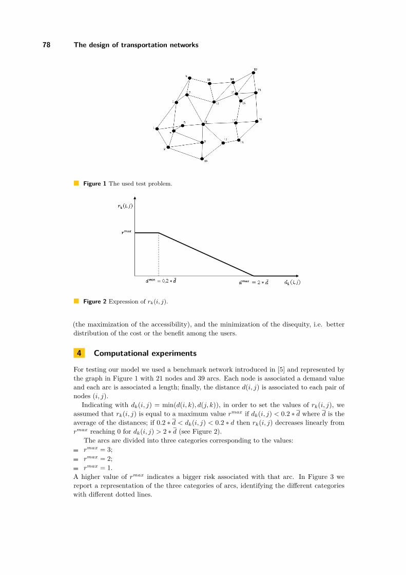
78 The design of transportation networks
Figure 1 The used test problem.
Figure 2 Expression of rk(i, j).
(the maximization of the accessibility), and the minimization of the disequity, i.e. betterdistribution of the cost or the benefit among the users.
4 Computational experiments
For testing our model we used a benchmark network introduced in [5] and represented bythe graph in Figure 1 with 21 nodes and 39 arcs. Each node is associated a demand valueand each arc is associated a length; finally, the distance d(i, j) is associated to each pair ofnodes (i, j).
Indicating with dk(i, j) = min(d(i, k), d(j, k)), in order to set the values of rk(i, j), weassumed that rk(i, j) is equal to a maximum value rmax if dk(i, j) < 0.2 ∗ d where d is theaverage of the distances; if 0.2 ∗ d < dk(i, j) < 0.2 ∗ d then rk(i, j) decreases linearly fromrmax reaching 0 for dk(i, j) > 2 ∗ d (see Figure 2).
The arcs are divided into three categories corresponding to the values:rmax = 3;rmax = 2;rmax = 1.
A higher value of rmax indicates a bigger risk associated with that arc. In Figure 3 wereport a representation of the three categories of arcs, identifying the different categorieswith different dotted lines.
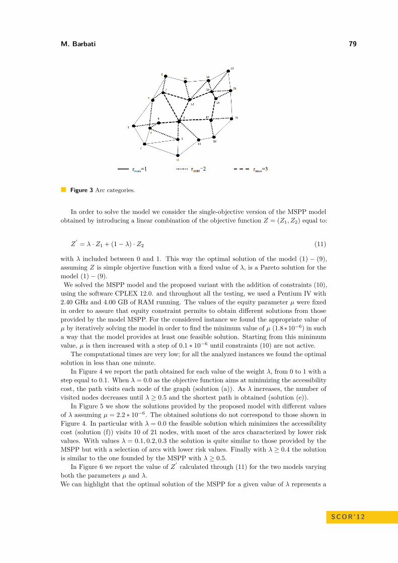
M. Barbati 79
Figure 3 Arc categories.
In order to solve the model we consider the single-objective version of the MSPP modelobtained by introducing a linear combination of the objective function Z = (Z1, Z2) equal to:
Z′ = λ · Z1 + (1− λ) · Z2 (11)
with λ included between 0 and 1. This way the optimal solution of the model (1) − (9),assuming Z is simple objective function with a fixed value of λ, is a Pareto solution for themodel (1)− (9).We solved the MSPP model and the proposed variant with the addition of constraints (10),using the software CPLEX 12.0. and throughout all the testing, we used a Pentium IV with2.40 GHz and 4.00 GB of RAM running. The values of the equity parameter µ were fixedin order to assure that equity constraint permits to obtain different solutions from thoseprovided by the model MSPP. For the considered instance we found the appropriate value ofµ by iteratively solving the model in order to find the minimum value of µ (1.8∗10−6) in sucha way that the model provides at least one feasible solution. Starting from this minimumvalue, µ is then increased with a step of 0.1 ∗ 10−6 until constraints (10) are not active.
The computational times are very low; for all the analyzed instances we found the optimalsolution in less than one minute.
In Figure 4 we report the path obtained for each value of the weight λ, from 0 to 1 with astep equal to 0.1. When λ = 0.0 as the objective function aims at minimizing the accessibilitycost, the path visits each node of the graph (solution (a)). As λ increases, the number ofvisited nodes decreases until λ ≥ 0.5 and the shortest path is obtained (solution (e)).
In Figure 5 we show the solutions provided by the proposed model with different valuesof λ assuming µ = 2.2 ∗ 10−6. The obtained solutions do not correspond to those shown inFigure 4. In particular with λ = 0.0 the feasible solution which minimizes the accessibilitycost (solution (f)) visits 10 of 21 nodes, with most of the arcs characterized by lower riskvalues. With values λ = 0.1, 0.2, 0.3 the solution is quite similar to those provided by theMSPP but with a selection of arcs with lower risk values. Finally with λ ≥ 0.4 the solutionis similar to the one founded by the MSPP with λ ≥ 0.5.
In Figure 6 we report the value of Z ′ calculated through (11) for the two models varyingboth the parameters µ and λ.We can highlight that the optimal solution of the MSPP for a given value of λ represents a
SCOR’12
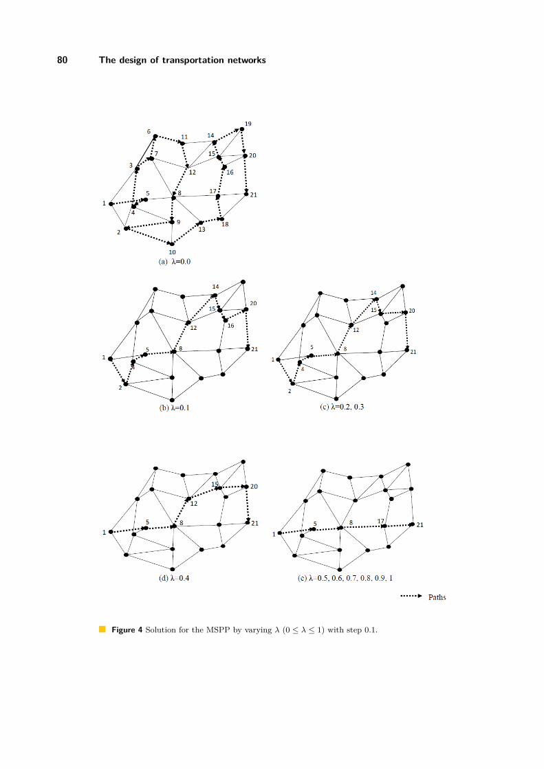
80 The design of transportation networks
Figure 4 Solution for the MSPP by varying λ (0 ≤ λ ≤ 1) with step 0.1.
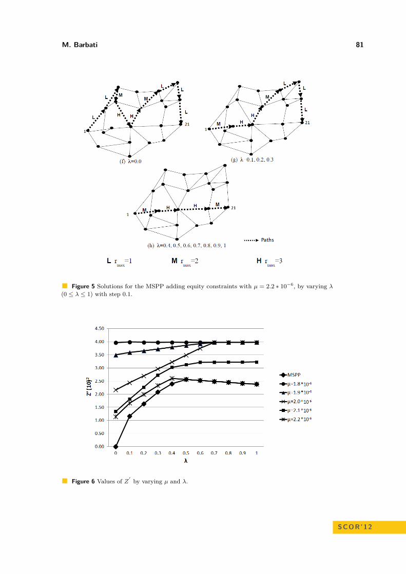
M. Barbati 81
Figure 5 Solutions for the MSPP adding equity constraints with µ = 2.2 ∗ 10−6, by varying λ(0 ≤ λ ≤ 1) with step 0.1.
Figure 6 Values of Z′
by varying µ and λ.
SCOR’12

82 The design of transportation networks
lower bound for Z when the equity constraint is introduced. When µ decreases we obtainsolutions with significant difference from the lower bound due to the fact that the set ofequity constraints is more active and then its presence reduces the set of feasible solutions.For example analyzing the obtained solution for λ = 0.5 for the lowest value of µ, and so forthe highest level of equity, the solution is characterized by a higher value of Z ′ . Increasing µ,and so decreasing the level of the equity, also the level of Z ′ decrease; so, the solution forintermediate values of µ are characterized by both level of equity and Z ′ (representing of theother two objectives), as wished. In addition, decrementing the level of equity the solutionbecomes more similar to those obtained by the MSPP model, until when µ ≥ 2.3 for whichthe solutions of the proposed model correspond with ones provided by the MSPP model forall the values of λ; in practice the constraint is not more effective.
5 Conclusion
In this work we analyzed the path location problems, taking into account the three mainmodels in the literature: the Median Shortest Path Problem (MSPP), the Maximum CoveringShortest Path Problem (MCSPP) and the Equity Constrained Shortest Path problem. Fromthe analysis of the literature we found the opportunity to include equity aspects in this context.For this reason we proposed a variant of the MSPP introducing balancing constraints. Weformulated the model and we tested its effectiveness through experiments on a test problem.Comparing the solutions, it became evident the effect of the insertion of the equity constraintson the resulting paths; indeed we found paths with a higher level of equity and also withgood values of the other two objectives. As further research we want to seek alternativemethods of calculating the perceived risk from each node, in order to adapt the model todescribe different applications.
Acknowledgements I would like to thank Riccardo Palladino for the work completed duringhis degree thesis from which this work originates and my supervisor Giuseppe Bruno forhelping me to develop this work and also this paper.
References1 B. Boffey Multiobjective Routing Problems. Top, vol.3, pp. 167-203, 1995.2 J.R. Current. Multiple objectives in transportation network design and routing. European
Journal of Operational Research vol.65, pp. 1-3, 1993.3 J. Current, M.Marsh. Multiobjective transportation network design and routing prob-
lems:Taxonomy and annotation. European Journal of Operational Research vol.65, pp. 4-19,1993.
4 J.R. Current , C.S. Revelle, J.L. Cohon. The maximum covering/shortest path problem: amultiobjective network design and routing formulation. European Journal of OperationalResearch, vol. 21, pp. 189-199, 1985.
5 J.R. Current , C.S. Revelle, J.L. Cohon. The median shortest path problem: a multiob-jective approach to analyze cost vs. accessibility in the design of transportation networks.Transportation Science, vol. 21, pp. 188-197, 1987.
6 M. Ehrgott, X. Gandibleux A survey and annotated bibliography of multiobjective com-binatorial optimization. Operations Research Spektrum, vol. 22, pp. 425-460, 2000.
7 H.A. Eiselt, G. Laporte Objectives in Location Problems. In: Facility Location: A Surveyof Applications and Methods, pp.151-180,Springer-Verlag, Berlin, 1995.
8 R.Z. Farahani, M. SteadieSeifi, N. Asgari. Multiple criteria facility location problems: Asurvey. Applied Mathematical Modelling, vol. 34, 1689-1709, 2008.

M. Barbati 83
9 R. Gopalan, R. Batta, M.H. Karwan . The Equity Constrained Shortest Path Problem.Computers & Operations Research, vol.17, pp. 297-307, 1990.
10 R. Gopalan, K.S. Kolluri, R. Batta, M.H. Karwan. Modeling equity of risk in the trans-portation of hazardous materials. Operations Research, vol.38, pp. 961-973, 1990.
11 M.B. Mandell. Modelling Effectiveness-Equity Trade-Offs in Public Service Delivery Sys-tems. Management Science, vol. 37, pp. 467-482, 1991.
SCOR’12
Heuristics for the routing of trucks with doublecontainer loads∗
Michela Lai1, Massimo Di Francesco2, and Paola Zuddas3
1 Department of Mathematics and Computer Science, University of CagliariVia Ospedale 72, 09124, Cagliari, [email protected]
2 Department of Land Engineering, University of CagliariVia Marengo 2, 09123, Cagliari, [email protected]
3 Department of Mathematics and Computer Science, University of CagliariVia Ospedale 72, 09124, Cagliari, [email protected]
AbstractThis research addresses a problem motivated by a real case study. A carrier must plan theroutes of trucks in order to serve importers and exporters. What is original in this vehiclerouting problem is the impossibility to separate trucks and containers during customer serviceand the opportunity to carry up to two containers per truck. Customers may demand more thanone container and may be visited more than once. Moreover, according to the carrier’s policy,importers must be served before exporters. In order to address this Vehicle Routing Problemwith backhaul and splits, a linear integer programming model is proposed. This research aimsto show to what extent an exact algorithm of a state of the art solver can be used to solve thismodel. Moreover, since some instances are too difficult to solve for the exact algorithm, a numberof heuristics is proposed and compared to this algorithm. Finally, the heuristics are compared tothe real decisions of the carrier who has motivated this problem.
1998 ACM Subject Classification H.4.2 Types of Systems Logistics
Keywords and phrases Split Vehicle Routing Problem, Backhaul, Drayage, Container transport-ation, Heuristics
Digital Object Identifier 10.4230/OASIcs.SCOR.2012.84
1 Introduction
This paper addresses a vehicle routing problem, which is motivated by a real case study. Acarrier is in charge of planning the distribution of container loads by trucks and containersbased at a port. The carrier has a homogeneous fleet of trucks carrying up to two containersand the planning of routes must be performed within 10 minutes. Two classes of customersmust be served: importers and exporters. The importers need to receive full container loadsfrom the port and the exporters need to ship container loads to the port. Typically customersneed to be served by more than one container and must be visited by more than one truck.
According to the carrier’s policy, trucks and containers cannot be uncoupled duringcustomer service, because truck drivers are required to check the right execution of operations.As a result, in this problem there are no pickups or deliveries of loaded and empty containers:
∗ This work was partially supported by Grendi Trasporti Marittimi.
© Michela. Lai, Massimo Di Francesco, and Paola Zuddas;licensed under Creative Commons License NC-ND
3rd Student Conference on Operational Research (SCOR 2012).Editors: Stefan Ravizza and Penny Holborn; pp. 84–93
OpenAccess Series in InformaticsSchloss Dagstuhl – Leibniz-Zentrum für Informatik, Dagstuhl Publishing, Germany
M. Lai, M. Di Francesco, and P. Zuddas 85
during customer service containers are filled or emptied and moved away by the same trucksused for bringing containers to customers.
Moreover, since the container loads of exporters are typically not ready before theafternoon, the carrier policy is to serve importers before exporters. As a result, emptycontainers leaving from importers can be moved to exporters, where they are filled andshipped to the port.
This problem belongs to the class of Vehicle Routing Problem (VRP) with backhauls,because deliveries must be performed before pickups [1]. However, in classical VRP withbackhaul each customer must be visited only once, whereas in our problem multiple visits ateach customer are allowed. Therefore, although several solution methods exist in VRP withbackhauls [2], [3], [4], [5], they may be suboptimal because splits are not considered.
There are also some similarities to drayage problems, which consists of picking up anddelivering of full containers. Typically they are separated from trucks during customer service[6], whereas this is not possible in this problem. The closest problem setting was probablyfaced by Imai et al. [7], who studied the optimal assignment of own and chartered trucksto a set of delivery and pickup pairs. As in our setting, tractors and containers cannot beuncoupled, but the capacity of trucks is limited to one container only. Homogeneous fleetswith one container trucks are also considered in [8] and [9].
The objective of this paper is to propose an optimization model accounting for theoriginal characteristics of this problem. The model minimizes distribution costs, such that allcustomers are served as requested, truck capacity constraints hold and importers are servedbefore exporters.
Since we are required to determine efficient solutions rapidly, this paper also aims topropose a number of heuristics for this problem. The common idea between these heuristicsis to build an initial set of routes in which all customers are either importers or exporters.Next, these routes are merged according to different criteria, one for each heuristic.
The contributions of this paper are:to present a problem with some original characteristics, which have not been investigatedin the rich VRP literature;to model the problem by a linear integer programming formulation;to propose and evaluate a number of heuristics with respect to an exact algorithm of astate-of-art solver.
The paper is organized as follows. In Section 2 the problem description is presented. Theproblem is modeled in Section 3. Solution methods are described in Section 4. The heuristicsare tested in Section 5. Section 6 presents a summary of conclusions and describes futureresearch perspectives in the field.
2 Problem description
Consider a fleet of trucks and containers based at a port. Trucks carry up to two containersand serve two types of customer requests: the delivery of container loads from the port toimporters and the shipment of container loads from exporters to the same port. Typicallycustomers need to ship or receive more than one container load. Therefore, usually eachcustomer must be served by multiple containers and must be visited more than once.
A relevant characteristic of this problem is the impossibility to separate trucks andcontainers during customer service. As a result, when importers receive container loadsby trucks, containers are emptied and moved away by the same trucks used for providing
SCOR’12
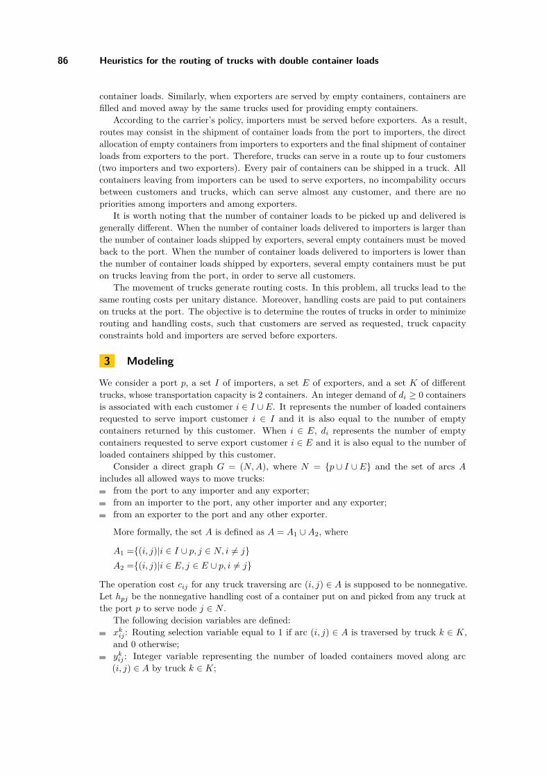
86 Heuristics for the routing of trucks with double container loads
container loads. Similarly, when exporters are served by empty containers, containers arefilled and moved away by the same trucks used for providing empty containers.
According to the carrier’s policy, importers must be served before exporters. As a result,routes may consist in the shipment of container loads from the port to importers, the directallocation of empty containers from importers to exporters and the final shipment of containerloads from exporters to the port. Therefore, trucks can serve in a route up to four customers(two importers and two exporters). Every pair of containers can be shipped in a truck. Allcontainers leaving from importers can be used to serve exporters, no incompability occursbetween customers and trucks, which can serve almost any customer, and there are nopriorities among importers and among exporters.
It is worth noting that the number of container loads to be picked up and delivered isgenerally different. When the number of container loads delivered to importers is larger thanthe number of container loads shipped by exporters, several empty containers must be movedback to the port. When the number of container loads delivered to importers is lower thanthe number of container loads shipped by exporters, several empty containers must be puton trucks leaving from the port, in order to serve all customers.
The movement of trucks generate routing costs. In this problem, all trucks lead to thesame routing costs per unitary distance. Moreover, handling costs are paid to put containerson trucks at the port. The objective is to determine the routes of trucks in order to minimizerouting and handling costs, such that customers are served as requested, truck capacityconstraints hold and importers are served before exporters.
3 Modeling
We consider a port p, a set I of importers, a set E of exporters, and a set K of differenttrucks, whose transportation capacity is 2 containers. An integer demand of di ≥ 0 containersis associated with each customer i ∈ I ∪ E. It represents the number of loaded containersrequested to serve import customer i ∈ I and it is also equal to the number of emptycontainers returned by this customer. When i ∈ E, di represents the number of emptycontainers requested to serve export customer i ∈ E and it is also equal to the number ofloaded containers shipped by this customer.
Consider a direct graph G = (N, A), where N = {p ∪ I ∪ E} and the set of arcs A
includes all allowed ways to move trucks:from the port to any importer and any exporter;from an importer to the port, any other importer and any exporter;from an exporter to the port and any other exporter.
More formally, the set A is defined as A = A1 ∪A2, where
A1 ={(i, j)|i ∈ I ∪ p, j ∈ N, i 6= j}A2 ={(i, j)|i ∈ E, j ∈ E ∪ p, i 6= j}
The operation cost cij for any truck traversing arc (i, j) ∈ A is supposed to be nonnegative.Let hpj be the nonnegative handling cost of a container put on and picked from any truck atthe port p to serve node j ∈ N .
The following decision variables are defined:xk
ij : Routing selection variable equal to 1 if arc (i, j) ∈ A is traversed by truck k ∈ K,and 0 otherwise;yk
ij : Integer variable representing the number of loaded containers moved along arc(i, j) ∈ A by truck k ∈ K;

M. Lai, M. Di Francesco, and P. Zuddas 87
zkij : Integer variable representing the number of empty containers moved along arc
(i, j) ∈ A by truck k ∈ K.
The problem can be formulated as follows:
min∑k∈K
∑(i,j)∈A
cijxkij +
∑j∈N
hpj(ykpj + zk
pj)
(1)
s.t. ∑k∈K
∑l∈N
ykil =
∑k∈K
∑j∈p∪I
ykji − di ∀i ∈ I (2)
∑k∈K
∑l∈N
zkil =
∑k∈K
∑j∈p∪I
zkji + di ∀i ∈ I (3)
∑l∈N
ykil ≤
∑j∈p∪I
ykji ∀i ∈ I, ∀k ∈ K (4)
∑l∈N
zkil ≥
∑j∈p∪I
zkji ∀i ∈ I, ∀k ∈ K (5)
∑k∈K
∑l∈p∪E
ykil =
∑k∈K
∑j∈N
ykji + di ∀i ∈ E (6)
∑k∈K
∑l∈p∪E
zkil =
∑k∈K
∑j∈N
zkji − di ∀i ∈ E (7)
∑l∈p∪E
ykil ≥
∑j∈N
ykji ∀i ∈ E,∀k ∈ K (8)
∑l∈p∪E
zkil ≤
∑j∈N
zkji ∀i ∈ E,∀k ∈ K (9)
ykij + zk
ij ≤ 2xkij ∀(i, j) ∈ A,∀k ∈ K (10)∑
j∈N
xkji −
∑l∈N
xkil = 0 ∀i ∈ N, ∀k ∈ K (11)
∑j∈N
xkpj ≤ 1 ∀k ∈ K (12)
∑k∈K
∑i∈I∪E
zkip −
∑k∈K
∑i∈I∪E
zkpi =
∑i∈I
di −∑i∈E
di (13)
xkij ∈ {0, 1} ∀(i, j) ∈ A,∀k ∈ K (14)
ykij ∈ {0, 1, 2} ∀(i, j) ∈ A,∀k ∈ K (15)
zkij ∈ {0, 1, 2} ∀(i, j) ∈ A,∀k ∈ K (16)
Container handling and truck routing costs are minimized in the objective function (1).Constraints from (2) to (5) concern the service to importers. Constraints (2) and (3)
are the flow conservation constraints of loaded and empty containers respectively at eachimporter node. Constraints (4) and (5) check the number of loaded and empty containers ineach truck entering and leaving from importers: when a truck leaves from each importer, thenumber of loaded containers cannot increase and the number of empty containers cannot bereduced.
Constraints from (6) to (9) concern the service to exporters. Constraints (6) and (7)are the flow conservation constraints of loaded and empty containers, respectively, for each
SCOR’12

88 Heuristics for the routing of trucks with double container loads
exporter node. Constraints (8) and (9) control the number of loaded and empty containersin each truck entering and leaving from exporters: when a truck leaves from each exporter,the number of loaded containers cannot be reduced and the number of empty containerscannot be increased.
Constraint (10) imposes that the number of containers moved by each truck is not largerthan the transportation capacity. Constraints (11) are the flow conservation constraints fortrucks at each node. Constraint (12) guarantees that trucks are not used more than once.Constraint (13) represents the flow conservation of empty containers at port p.
Finally, constraints (14), (15) and (16) define the domain of decision variables.
4 Solution methods
Several solution methods can be adopted to solve the previous problem. Generally speaking,they can be divided into exact and heuristic methods. In this paper we illustrate to whatextent a well-known exact algorithm can be used to face this problem. This analysis isperformed by the solver Cplex, which solves integer programming models by a branch-and-cutalgorithm.
However, most Vehicle Routing Problems are NP-hard and, also in our problem, there islittle hope of finding exact solution procedures for large problem instances [11]. Therefore,in this section we propose a number of heuristics, which can be used to tackle the problemat hand.
All proposed heuristics are composed of two phases. The first phase, which is the samefor all heuristics, determines an initial solution, in which all routes serve either importersor exporters. In the second phase, each heuristic implements a different rule to merge theroutes determined in the first phase. Finally, the best heuristic in terms of objective functionis selected.
In the first phase, we face two vehicle routing problems with splits: the first has importersonly, whilst the second has exporters only. However, Split Vehicle Routing Problems are alsoknown to be difficult. Therefore, since an efficient metaheuristic for this class of problemshas been proposed by Archetti et al. [10], their algorithm has been chosen to determineroutes in the first phase.
The routes determined in the first phase are merged in the second phase according todifferent saving-based heuristics. Savings represent the routing costs achieved by mergingtwo routes instead of leaving them separately. Given a route i with importers only and aroute j with exporters only, the saving generated by their merging is computed as sij =c(i) + c(j)− c(ij), in which c(i) and c(j) are the respective costs of routes i and j, and c(ij)is the cost of the merged route. Savings are saved in a matrix, in which the number of rowsis equal to the number of routes serving importers in the first phase and the number ofcolumns is equal to the number of routes serving exporters in the first phase.
In this paper, the order of visits between pairs of importers and pairs of exporters is notchanged after the merging. To clarify, let us consider for instance two importers i1 and i2and two exporters e1, e2. Assume that the routes determined in the first phase are p, i1, i2,p and p, e1, e2, p. If these routes are merged, the final route is p, i1, i2, e1, e2,p. Therefore,the possibility of visiting importer i2 before importer i1 and exporter e2 before e1 is nottaken into account.
Some definitions are provided for the sake of clarity in the presentation of the heuristics:Row i represents the i− th route of importers, as determined in the first phase;Column j represents the j − th route of exporters, as determined in the first phase;

M. Lai, M. Di Francesco, and P. Zuddas 89
Entry sij >= 0 is the saving generated by the merging of routes i and j. Only nonnegativesavings are considered. When an entry sij takes value 0, the merging is not allowed.Whenever two routes i and j are merged by a heuristic, the related saving sij is set to 0;
mi Number of columns (routes) that can be merged with the route represented by row i;mj Number of rows (routes) that can be merged with the route represented by column j;avrgi is the average of all savings in row i;avrgj is the average of all savings in column j.
We propose eight heuristics, whose solution is denoted by s0,...,7:Heuristic 0 (H0) This heuristic does nothing and returns routes as determined in the first
phase:Step0 s0 = ∅.Step1 For each row i, insert i into s0.Step2 For each column j, insert j into s0.
Heuristic 1 (H1) This heuristic determines the maximum saving for each route of importersand selects the best routes serving exporters:Step0 s1 = ∅.Step1 For each row i, select the largest sij . Merge routes i and j, if any, and insert the
new route into s1.Step2 For each row i not involved in any merging, insert i into s1.Step3 For each column j not involved in any merging, insert j into s1.
Heuristic 2 (H2) This heuristic determines the maximum saving for each route of exportersand selects the best routes serving importers:Step0 s2 = ∅.Step1 For each column j, select the largest sij . Merge routes i and j, if any, and insert
the new route into s2.Step2 For each row i not involved in any merging, insert i into s2.Step3 For each column j not involved in any merging, insert j into s2.
Heuristic 3 (H3) This heuristic gives priority to routes of importers that can be mergedwith a low number of other routes.Step0 s3 = ∅.Step1 Search for row i with the lowest value of mi. If any, go to Step2, otherwise go to
Step3.Step2 Select the largest sij for i, merge routes i and j and insert the new route into s3.
Go to Step1.Step3 For each row i not involved in any merging, insert i into s3.Step4 For each column j not involved in any merging, insert j into s3.
Heuristic 4 (H4) This heuristic gives priority to routes of exporters that can be mergedwith a low number of other routes.Step0 s4 = ∅.Step1 Search for column j with the lowest value of mj . If any, go to Step2, otherwise
go to Step3.Step2 Select the largest sij for j, merge routes i and j and insert the new route into s4.
Go to Step1.Step3 For each row i not involved in any merging, insert i into s4.Step4 For each column j not involved in any merging, insert j into s4.
SCOR’12

90 Heuristics for the routing of trucks with double container loads
Heuristic 5 (H5) This heuristic gives priority to routes of both importers and exporters,that can be merged with a low number of other routes:Step0 s5 = ∅.Step1 Search for row i with the lowest value of mi and the column j with the lowest
value of mj . If mi <= mj , go to Step2, otherwise go to Step3. If no routes can bemerged, go to Step4.
Step2 Select the largest sij for i, merge routes i and j and insert into s5. Go to Step1.Step3 Select the largest sij for j, merge routes i and j and insert into s5. Go to Step1.Step4 For each row i not involved in any merging, insert i into s5.Step5 For each column j not involved in any merging, insert j into s5.
Heuristic 6 (H6) This heuristic differs from the previous one in the selection of savings: wechoose the closest saving to the average of all available savings, instead of the largest one:Step0 s6 = ∅.Step1 Search for row i with the lowest value of mi and the column j with the lowest
value of mj . If mi <= mj , go to Step2, otherwise go to Step3. If no routes can bemerged, go to Step4.
Step2 Select the closest sij to avrgi, merge routes i and j and insert into s6. Go toStep1.
Step3 Select the closest sij to avrgj , merge routes i and j and insert into s6. Go toStep1.
Step4 For each row i not involved in any merging, insert i into s6.Step5 For each column j not involved in any merging, insert j into s6.
Heuristic 7 (H7) This heuristic merges the routes with the largest saving in the matrix:Step0 s7 = ∅.Step1 Select for the largest sij in the saving matrix. If any, go to Step2, otherwise go
to Step3.Step2 Merge routes i and j and insert the new route into s7. Go to Step1.Step3 For each row i not involved in any merging, insert i into s7.Step4 For each column j not involved in any merging, insert j into s7.
After the execution of all heuristics, we select the best one in terms of objective function.
5 Experimentation
In this section we test the previous heuristics on artificial and real instances. The realinstances are provided by a shipping company operating in the port of Genoa (Italy).
Tests are performed on both artificial and real instances. Five classes of artificial instanceshave been generated:
10 customers;20 customers;30 customers;40 customers;50 customers.
In each class the coordinates of nodes are fixed. The instances of a class differ in thenumber of importers and exporters. The heuristics are implemented in the programminglanguage C++. Tests are performed by Cplex 12.2 running on a four-CPU server 2.67 GHz

M. Lai, M. Di Francesco, and P. Zuddas 91
64 GB RAM. Since a major requirement of this problem is to determine solutions in a fewminutes, Cplex is set to stop after 10 minutes. Computational results are indicated in Table2, in which the following notation is used:|I|: Number of importers;|E|: Number of exporters;H0, . . . , H7: Objective function returned by Heuristic 0,. . . , Heuristic 7;t(s): The total execution time (in seconds) to solve the related instance, i.e. it representshow long it takes to run the first phase plus the time spent to run all heuristics H0, . . . ,H7;% Gap from CPLEX : gap between the best heuristic and the best upper bound providedby CPLEX within 10 minutes;Optimality gap: Optimality gap between lower and upper bounds in Cplex after 10minutes.
The string n.s. means that Cplex cannot provide a feasible solution within 10 minutes.Table 2 shows that only one instance with 10 customers can be optimally solved. Cplex
does not provide feasible solutions within 10 minutes for all instances with 40 and 50customers, whereas all heuristics can solve these instances within 10 minutes. Generallyspeaking, the heuristic H7 is the most promising in terms of the objective function.
Real instances, which have about 40 customers, have no feasible solutions by Cplex within10 minutes. In this case we compare the best heuristic to the carrier’s decisions in terms oftotal travelled distances. Results on the real instances are shown in Table 1, in which thefollowing notation is used:
Instances The instance considered;|I| Number of importers;|E| Number of exporters;|K| Number of trucks;Carrier’s decisions The total travelled distance according to the carrier’s decisions (km);Decisions The total travelled distance according to the best heuristic (km);% Improvement: gap between the best heuristic and the carrier’s decisions;Criterion The heuristic(s) providing the best solution;
Table 1 The solutions of real instances.
Instances |I| |E| |K| Carrier’s Best Heuristicdecisions Decisions % Improvement Criterion
Instance 1 7 34 41 16503 16196 -1.90 7Instance 2 10 28 31 13369 11701 -14.26 7Instance 3 3 31 39 13702 13602 -0.74 1, 3, 7Instance 4 6 34 36 13263 12328 -7.58 7Instance 5 3 28 41 13180 12869 -2.42 1, 3, 7
Table 1 shows that in each instance the best heuristic always improves the carrier’sdecisions. The improvement seems to be particularly relevant when |I| increases and becomescloser to |E|, due to the larger search space of feasible routes.
SCOR’12
92 Heuristics for the routing of trucks with double container loads
6 Conclusion
This paper has investigated a vehicle routing problem with some original characteristics, suchas the opportunity to carry two containers per truck and the impossibility to separate trucksand containers during customer service. We have formulated an integer linear programmingmodel for this problem. An exact algorithm was used to solve several artificial instances,but it was able to solve only instances with few customers. Several heuristics are proposedand tested on both artificial and real instances. According to our tests, the most promisingheuristic in terms of objective function is H7, because high-quality routes are built from thebeginning by the maximum saving.
The comparison with the carrier’s decisions shows that the heuristics represent a promisinginstrument to improve its current decision-making process, because they yield significantsavings in distances travelled by trucks.
Research is in progress to face problems with heterogeneous fleets of trucks, time windowsand larger transportation capacities. New heuristics will be developed accounting for thespecific characteristics of these problems.
Acknowledgements The authors want to thank professor Claudia Archetti, who madeavailable her Tabu Search code for the Split Vehicle Routing Problem. The authors are alsograteful to Antonio Musso, managing director of Grendi Trasporti Marittimi, who introducedto them the application that motivated this research.
References1 P. Toth, D. Vigo. The Vehicle Routing Problem. SIAM Monographs on Discrete Mathem-
atics and Applications, Philadelphia, USA, 2002.2 S. Anily. The Vehicle Routing Problem with Delivery and Back-haul Options. Naval Re-
search Logistic Quarterly, 43, 415-434, 1996.3 A. Mingozzi, S. Giorgi and R. Baldacci. An Exact Method for the Vehicle Routing Problem
with Backhauls. Transportation Science, 33, 315-329, 1999.4 P. Toth, D. Vigo. An Exact Algorithm for the Vehicle Routing Problem with Backhauls.
Transportation Science, 31, 372-385, 1997.5 P. Toth, D. Vigo. A Heuristic Algorithm for the Symmetric and Asymmetric Vehicle Rout-
ing Problem with Backhauls. European Journal of Operational Research, 113, 528-543,1999.
6 R. Zhang, W.Y. Yun, I.K. Moon. Modeling and optimization of a container drayage problemwith resource constraints. International Journal of Production Economics, 133, 351-359,2011.
7 A. Imai, E. Nishimura, J. Current. A Lagrangian relaxation-based heuristic for the vehiclerouting with full container load. European Journal of Operational Research, 176, 87-105,2007.
8 A. Caris, G.K. Janssens. A Local search heuristic for the pre- and end-haulage of intermodalcontainer terminals. Computers and Operations Research, 36, 2763-2772, 2009.
9 R. Namboothiri and A.L. Erera, Planning local container drayage operations given a portaccess appointment system. Transportation Research Part E: Logistics and TransportationReview, 44, 185-202, 2008.
10 C. Archetti, M. G. Speranza, A. Hertz. A Tabu Search Algorithm for the Split DeliveryVehicle Routing Problem. Transportation science, 40, 1, 64-73, 2006.
11 C. H. Papadimitriou. Computational Complexity. Addison Wesley Longman, 1993.
M. Lai, M. Di Francesco, and P. Zuddas 93
Table2The
solutio
nsof
artifi
cial
instan
ces.
HEURISTIC
SCPLE
X
|I|
|E|
H0
H1
H2
H3
H4
H5
H6
H7
t(s)
%Gap
from
CPLE
X
%Optim
ality
Gap
10CLIENTS
28
2417
0.26
2087
2.07
2139
2.98
2067
2.07
2139
2.98
2298
5.55
2298
5.55
2067
2.07
60.00
4.06
55
2367
4.27
2154
4.40
2091
6.21
2241
1.33
20066.19
2072
9.28
2113
1.93
1996
0.83
00.00
0.00
82
2406
7.78
2352
8.75
2110
9.77
2317
5.59
2110
9.77
2128
9.41
2286
3.04
2110
9.77
01.95
4.04
20CLIENTS
218
4643
6.64
4156
6.04
4363
9.35
4076
6.04
4363
9.35
4331
9.77
4331
5.09
4076
6.04
0-2.93
7.51
515
4620
4.46
3687
3.01
4274
3.03
3623
3.01
4184
5.95
4063
6.38
4037
8.63
3623
3.01
0-4.48
7.91
1010
4632
6.75
3475
1.04
3625
6.89
3527
7.56
36608.49
3597
6.40
3812
7.17
3309
2.29
04.20
4.40
155
4620
4.46
4002
1.52
3733
6.19
4022
2.93
38196.39
4048
0.64
4246
3.88
3726
1.67
0-1.08
6.29
182
4620
4.46
4401
9.68
4305
0.79
4487
7.00
43050.79
4445
9.09
4475
3.25
4297
5.11
42-2.41
7.02
30CLIENTS
228
6912
1.47
6370
8.18
6675
0.74
6272
8.18
6673
0.74
6687
1.79
6668
2.33
6272
8.18
3-6.38
9.52
525
6990
6.97
6001
9.63
6636
5.54
5942
3.33
65468.45
6480
9.86
6686
3.83
5935
9.63
2-1.76
6.66
1020
7070
4.03
5477
4.37
6057
4.18
5474
0.43
59587.76
5858
1.67
6404
7.55
5412
9.24
1-5.63
14.27
1515
7090
5.38
5209
2.61
5093
4.97
5268
7.38
53340.51
5117
2.63
6081
6.68
4921
8.46
1-4.44
10.37
2010
7090
5.38
5917
0.97
5500
4.74
6057
6.35
55574.39
5899
8.61
6380
8.75
5475
7.12
1n.s
n.s.
255
6948
1.27
6669
5.13
6107
5.33
6655
4.36
61075.33
6453
8.63
6597
7.58
6107
4.67
2-13.11
15.51
282
6898
2.30
6990
6.35
6721
7.27
6856
3.65
6721
7.27
6836
1.82
6836
1.82
6721
7.27
3-5.17
9.93
40CLIENTS
238
1013
02.11
9564
5.86
9969
5.34
9398
5.86
1000
62.51
9629
1.21
9695
2.05
9398
5.86
17n.s
n.s.
535
1018
52.55
8876
4.09
9165
4.05
8824
4.09
9205
3.54
9549
8.95
9940
1.32
8822
4.09
11n.s
n.s.
1030
1015
82.68
7619
4.52
8299
9.48
7596
8.82
8544
2.09
8662
1.65
9062
6.66
7511
7.98
49n.s
n.s.
1525
1017
76.10
7092
0.95
7601
6.82
7034
7.44
7551
8.30
7498
0.22
8936
8.12
6848
4.46
3n.s
n.s.
2020
1018
95.27
7652
5.84
7151
4.12
7694
1.13
7170
9.14
7564
1.02
8904
4.40
7079
5.53
2n.s
n.s.
2515
1023
49.92
8373
3.24
7674
9.41
8326
7.22
7680
5.40
8750
5.43
9538
7.34
7626
1.72
5n.s
n.s.
3010
1012
86.43
9183
8.75
8577
2.27
9256
0.11
8588
8.37
9185
1.87
9524
3.18
8550
6.14
6n.s
n.s.
355
1017
35.75
9905
7.56
9507
2.84
9782
8.28
9507
2.84
9809
5.70
1003
64.94
9507
2.84
11n.s
n.s.
382
1007
22.47
1002
65.05
9773
6.69
9951
6.60
9773
6.69
1001
09.32
1001
09.32
9773
6.69
11n.s
n.s.
50CLIENTS
248
1320
95.20
1252
33.97
1306
17.35
1245
13.9
713
0761
.45
1308
57.73
1309
59.03
1245
13.9
720
n.s
n.s.
545
1314
32.46
1206
17.96
1262
58.08
1201
97.9
612
5786
.41
1254
47.20
1283
93.50
1201
97.9
623
n.s
n.s.
1040
1320
98.19
1131
27.96
1160
88.33
1126
87.9
611
6348
.43
1204
67.73
1241
13.76
1126
87.9
615
n.s
n.s.
1535
1334
59.72
1023
04.67
1130
48.46
1007
70.4
811
3085
.01
1113
24.61
1215
95.94
1008
37.89
8n.s
n.s.
2030
1326
73.52
9427
9.48
9896
6.22
9208
9.72
1036
20.29
9957
5.14
1134
07.89
9154
2.11
5n.s
n.s.
2525
1318
59.53
8480
7.36
9131
8.81
8325
4.21
9280
7.30
8602
8.26
1121
55.51
8237
3.34
5n.s
n.s.
3020
1319
07.73
8985
4.06
8623
9.26
8810
5.14
8686
5.49
9023
7.42
1119
15.47
8392
3.10
6n.s
n.s.
3515
1320
79.70
1034
80.43
9640
5.91
1040
61.17
9667
2.63
1062
94.63
1170
55.94
9577
1.71
8n.s
n.s.
4010
1314
50.60
1142
21.90
1060
93.40
1167
02.34
1069
20.76
1154
79.38
1245
21.98
1059
76.9
210
n.s
n.s.
455
1327
93.70
1231
51.73
1130
13.98
1224
72.64
1142
08.57
1236
25.22
1247
87.33
1127
04.7
219
n.s
n.s.
482
1328
92.88
1279
84.28
1224
62.3
712
6229
.39
1224
62.3
712
8170
.93
1302
64.79
1224
62.3
735
n.s
n.s.
SCOR’12

Optimization of electricity trading using linearprogramming∗
Minja R. Marinović1, Dragana D. Makajić-Nikolić1,Milan J. Stanojević1, and Lena S. Ðorđević1
1 Faculty of organizational sciences, University of BelgradeJove Ilića 154, Belgrade, [email protected], [email protected], [email protected],[email protected]
AbstractIn the last two decades, the liberalization of the electricity markets have been established in orderto increase efficiency, harmonize and reduce electricity prices, make a better use of resources, givecustomers the right to choose their supplier and provide customers with a better service. Thischange made the electricity market competitive and introduced several new subjects. In thispaper, we study one of these subjects: Electricity Trading Company (ETC) and its daily tradingprocess. We present a linear mathematical model of total daily profit maximization subjectto flow constraints. It is assumed that the demand and supply are known and some of themare arranged. Possible transmission capacities are known but also additional capacities can bepurchased. All trading, transmission prices and amounts are subject of auctions. First, we presentenergy trading problem as directed multiple-source and multiple-sink network and then model itusing linear programming. Also, we provide one realistic example which is slightly changed inorder to save confidentiality of the given data.
1998 ACM Subject Classification G 1.6 Optimization, G 2.2 Network Problems
Keywords and phrases energy daily trading, day-ahead planning, LP model, optimization
Digital Object Identifier 10.4230/OASIcs.SCOR.2012.94
1 Introduction
Until the nineties, power plants power production and transmission were carried out betweenmonopolistic public power companies. This situation changed since electricity markets havebeen deregulated allowing customers to choose their provider and producers. Today, we have aSingle European electricity market which provides seamless competition within the electricitysupply chain. All participants enjoy a wide choice between competing electricity retailers,who source their requirements in competitive wholesale markets. Market participants aretrying to satisfy demand in their own countries and supply electricity across borders intoneighborhood markets. Cross-border trading and supply is a part of this market. EnergyTrading Companies (ETCs) are buying transmission capacity from Transmission SystemOperators (TSOs) [1]. All time, TSOs consistently release to the market a truly maximumamount of cross-border transmission capacity. We should mention that ETCs are operatingin the middle stage of an energy supply chain [11] and they are trying to manage the risksassociated with fluctuating prices through buying and selling electricity contracts. Both
∗ This research was partially supported by the Ministry of Education and Science, Republic of Serbia,Projects numbers TR32013 and TR35045.
© Minja R. Marinović, Dragana D. Makajić-Nikolić, Milan J. Stanojević, and Lena S. Ðorđević;licensed under Creative Commons License NC-ND
3rd Student Conference on Operational Research (SCOR 2012).Editors: Stefan Ravizza and Penny Holborn; pp. 94–102
OpenAccess Series in InformaticsSchloss Dagstuhl – Leibniz-Zentrum für Informatik, Dagstuhl Publishing, Germany

M.R. Marinović, D.D. Makajić-Nikolić, M.J. Stanojević, and L.S. Ðorđević 95
traders and end-users apply financial instruments such as futures, options and derivatives toprotect their exposures to prices and to speculate on price fluctuations.
There are few ways of trading electricity but two main ways are via the telephone inbilateral transactions (so called “Over The Counter“ or OTC, usually through the intermedi-ation of a broker), or it is traded through futures markets such as Nordpool or EEX. Somekey factors influencing energy prices include geopolitical factors, global economic growth,short term weather impacting demand, supply disruptions from maintenance or unexpectedoutages, fuel price movements and product swapping in response to relative prices [3].
The literature concerning different issues in energy trading and transmission is extensive.In [8] the authors analyze the impact of CO2 cost on power prices and test two differentaverage cost pricing policies, regional and zonal, that have different effects on electricitymarket of Central and West Europe. In [12] multiple interrelated markets is considered forelectricity and propose a multi-stage mixed-integer stochastic model for capacity allocationstrategy in a multi-auction competitive market. A generalized network flow model of thenational integrated energy system that incorporates production, transportation of coal,natural gas, and electricity storage with respect to the entire electric energy sector of theU.S. economy is proposed in [10]. The authors have formulated a multi period generalizedflow problem in which the total cost is minimized subject to energy balance constraints. Theproblem of energy allocation between spot markets and bilateral contracts is formulatedas a general portfolio optimization quadratic programming problem in [6]. The proposedmethodology with risky assets can be applied to a market where pricing, either zonal or nodal,is adopted to mitigate transmission congestion. In [9] the authors propose a zonal networkmodel, aggregating individual nodes within each zone into virtual equivalent nodes, and allcross-border lines into equivalent border links. Using flow-based modeling, the feasibility ofthe least granularity zonal model where the price zones are defined by the political borders,is analyzed. The authors in [4] consider network systems with multiple-source multiple-sinkflow such as electric and power systems. They observe the problem in which resources aretransmitted from resource-supplying nodes to resource-demanding nodes through unreliableflow networks. In [7] they analyze the simultaneous optimization of power production andday-ahead power trading and formulated it as a stochastic integer programming model.
In this paper, we consider day-ahead planning from the perspective of a decision makerin ETC. Decisions that should be made are: where and how much electricity ETC shouldbuy and sell and on which ways that energy should be transferred in order to maximizetotal daily profit. We represent this problem by a directed multiple-source and multiple-sinknetwork and model using linear programming. We illustrate this approach on an example ofone ETC trading on Central and South-East Europe (CSEE).
The paper is organized as follows. Section 2 is devoted to a description of the mainassumptions of the observed problem. In Section 3, we present a LP model for day-aheadplanning. Then, in Section 4 we report and discuss numerical results to illustrate the modelapplication. Also, we present the solution of the LP model with fixed parameters and thenwe investigate the impact of prices on trading capacities and amounts. Conclusions alongwith perspectives regarding further work are given in Section 5.
2 Problem description
In this paper we are focusing on electricity trading from the perspective of ETC. The maintask of trading section of ETC is to ensure each client’s demands are met whatever thecircumstances. Trading section also enables ETC to respond to the ever-changing state of the
SCOR’12
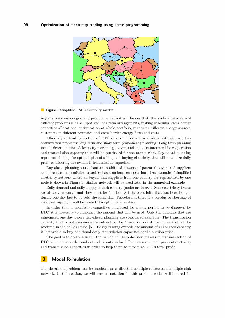
96 Optimization of electricity trading using linear programming
Figure 1 Simplified CSEE electricity market.
region’s transmission grid and production capacities. Besides that, this section takes care ofdifferent problems such as: spot and long term arrangements, making schedules, cross bordercapacities allocations, optimization of whole portfolio, managing different energy sources,customers in different countries and cross border energy flows and costs.
Efficiency of trading section of ETC can be improved by dealing with at least twooptimization problems: long term and short term (day-ahead) planning. Long term planninginclude determination of electricity market e.g. buyers and suppliers interested for cooperationand transmission capacity that will be purchased for the next period. Day-ahead planningrepresents finding the optimal plan of selling and buying electricity that will maximize dailyprofit considering the available transmission capacities.
Day-ahead planning starts from an established network of potential buyers and suppliersand purchased transmission capacities based on long term decisions. One example of simplifiedelectricity network where all buyers and suppliers from one country are represented by onenode is shown in Figure 1. Similar network will be used later in the numerical example.
Daily demand and daily supply of each country (node) are known. Some electricity tradesare already arranged and they must be fulfilled. All the electricity that has been boughtduring one day has to be sold the same day. Therefore, if there is a surplus or shortage ofarranged supply, it will be traded through future markets.
In order that transmission capacities purchased for a long period to be disposed byETC, it is necessary to announce the amount that will be used. Only the amounts that areannounced one day before day-ahead planning are considered available. The transmissioncapacity that is not announced is subject to the “use it or lose it” principle and will bereoffered in the daily auction [5]. If daily trading exceeds the amount of announced capacity,it is possible to buy additional daily transmission capacities at the auction price.
The goal is to create a useful tool which will help decision makers in trading section ofETC to simulate market and network situations for different amounts and prices of electricityand transmission capacities in order to help them to maximize ETC’s total profit.
3 Model formulation
The described problem can be modeled as a directed multiple-source and multiple-sinknetwork. In this section, we will present notation for this problem which will be used for
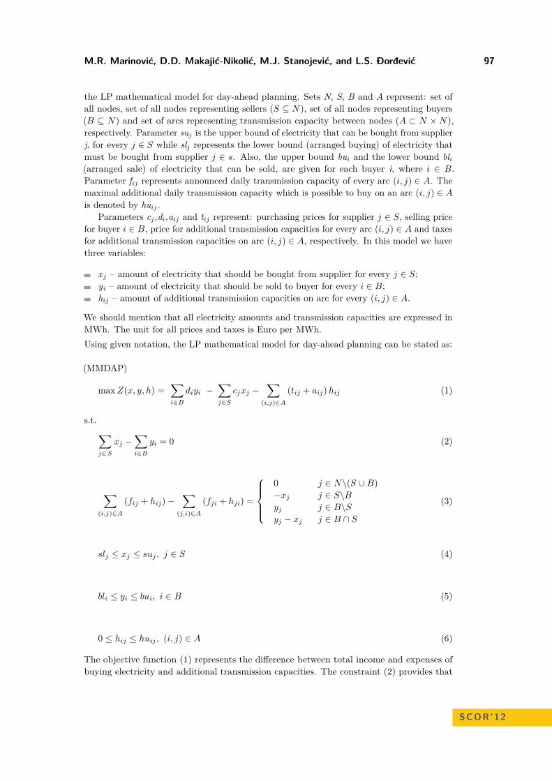
M.R. Marinović, D.D. Makajić-Nikolić, M.J. Stanojević, and L.S. Ðorđević 97
the LP mathematical model for day-ahead planning. Sets N, S, B and A represent: set ofall nodes, set of all nodes representing sellers (S ⊆ N), set of all nodes representing buyers(B ⊆ N) and set of arcs representing transmission capacity between nodes (A ⊂ N ×N),respectively. Parameter suj is the upper bound of electricity that can be bought from supplierj, for every j ∈ S while slj represents the lower bound (arranged buying) of electricity thatmust be bought from supplier j ∈ s. Also, the upper bound bui and the lower bound bli(arranged sale) of electricity that can be sold, are given for each buyer i, where i ∈ B.Parameter fij represents announced daily transmission capacity of every arc (i, j) ∈ A. Themaximal additional daily transmission capacity which is possible to buy on an arc (i, j) ∈ A
is denoted by huij .Parameters cj ,di,aij and tij represent: purchasing prices for supplier j ∈ S, selling price
for buyer i ∈ B, price for additional transmission capacities for every arc (i, j) ∈ A and taxesfor additional transmission capacities on arc (i, j) ∈ A, respectively. In this model we havethree variables:
xj – amount of electricity that should be bought from supplier for every j ∈ S;yi – amount of electricity that should be sold to buyer for every i ∈ B;hij – amount of additional transmission capacities on arc for every (i, j) ∈ A.
We should mention that all electricity amounts and transmission capacities are expressed inMWh. The unit for all prices and taxes is Euro per MWh.Using given notation, the LP mathematical model for day-ahead planning can be stated as:
(MMDAP)
max Z(x, y, h) =∑i∈B
diyi −∑j∈S
cjxj −∑
(i,j)∈A
(tij + aij) hij (1)
s.t. ∑j∈ S
xj −∑i∈B
yi = 0 (2)
∑(i,j)∈A
(fij + hij)−∑
(j,i)∈A
(fji + hji) =
0−xj
yj
yj − xj
j ∈ N\(S ∪B)j ∈ S\Bj ∈ B\Sj ∈ B ∩ S
(3)
slj ≤ xj ≤ suj , j ∈ S (4)
bli ≤ yi ≤ bui, i ∈ B (5)
0 ≤ hij ≤ huij , (i, j) ∈ A (6)
The objective function (1) represents the difference between total income and expenses ofbuying electricity and additional transmission capacities. The constraint (2) provides that
SCOR’12
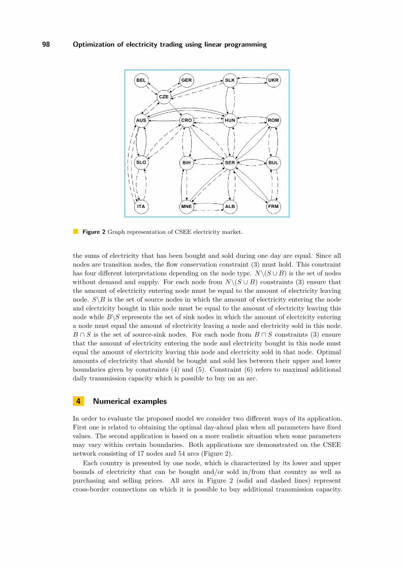
98 Optimization of electricity trading using linear programming
Figure 2 Graph representation of CSEE electricity market.
the sums of electricity that has been bought and sold during one day are equal. Since allnodes are transition nodes, the flow conservation constraint (3) must hold. This constrainthas four different interpretations depending on the node type. N\(S ∪B) is the set of nodeswithout demand and supply. For each node from N\(S ∪ B) constraints (3) ensure thatthe amount of electricity entering node must be equal to the amount of electricity leavingnode. S\B is the set of source nodes in which the amount of electricity entering the nodeand electricity bought in this node must be equal to the amount of electricity leaving thisnode while B\S represents the set of sink nodes in which the amount of electricity enteringa node must equal the amount of electricity leaving a node and electricity sold in this node.B ∩ S is the set of source-sink nodes. For each node from B ∩ S constraints (3) ensurethat the amount of electricity entering the node and electricity bought in this node mustequal the amount of electricity leaving this node and electricity sold in that node. Optimalamounts of electricity that should be bought and sold lies between their upper and lowerboundaries given by constraints (4) and (5). Constraint (6) refers to maximal additionaldaily transmission capacity which is possible to buy on an arc.
4 Numerical examples
In order to evaluate the proposed model we consider two different ways of its application.First one is related to obtaining the optimal day-ahead plan when all parameters have fixedvalues. The second application is based on a more realistic situation when some parametersmay vary within certain boundaries. Both applications are demonstrated on the CSEEnetwork consisting of 17 nodes and 54 arcs (Figure 2).
Each country is presented by one node, which is characterized by its lower and upperbounds of electricity that can be bought and/or sold in/from that country as well aspurchasing and selling prices. All arcs in Figure 2 (solid and dashed lines) representcross-border connections on which it is possible to buy additional transmission capacity.

M.R. Marinović, D.D. Makajić-Nikolić, M.J. Stanojević, and L.S. Ðorđević 99
Table 1 Optimal solution.
Buying in MWh Selling in MWhnode min Optimal max min Optimal maxBEL 18 40 40 25 31 67GER 2 70 70 0 70 80AUS 1 31 31 0 0 60ITA 0 36 50 31 41 41SLO – – – 5 5 35CZE 25 35 35 0 0 38HUN 0 0 10 – – –CRO – – – 22 22 44BiH 36 52 52 42 49 49MNE – – – 5 5 60SLK – – – 12 12 33SER 0 46 46 0 80 80ALB 5 10 35 – – –FRM 0 40 40 3 3 57ROM – – – 4 38 70BUL – – – 14 14 25UKR 10 10 20 – – –
Arcs represented by solid lines indicate the existence of announced transmission capacitiespurchased earlier. Maximal additional daily transmission capacities, amounts of announcedtransmission capacities, prices and taxes of each arc are also given. Due to confidentialityissues, we present in this paper slightly modified data which are within boundaries of commonreal-life situations.The model has been implemented and solved using the GNU Linear Programming Kit [2].The optimal solution for one scenario is given in Table 1. Marks “–” mean that there wereno suppliers or buyers in the corresponding country.In addition to the optimal trade amounts, the solution determines additional transmissioncapacities that should be purchased. As well, the solution provides information about totaltrade amounts in MWh and profit which will be made with this scenario.Beside information about total daily trade and total daily income, the application has thepossibility to show expenses of buying electricity and expenses of additional transmissioncapacities in Euros. In order to obtain a total profit certain corrections in the objective haveto be made:
Taxes for announced transmission capacities as well as costs of long term purchasedtransmission capacities evaluated on daily basis should be subtracted.Unit prices for previously arranged buying and selling (blj and slj) can differ from actualprices. These differences should be taken into account.
However, any of these corrections will not affect the optimal solution obtained by the model.In the further analysis we will use the term “profit” to refer to the value in (1), although itis just an approximation.In order to demonstrate the second way of using MMDAP we perform a sensitivity analysisfor some parameters. In this case we present a scenario where the selling price for node SERvaries from 80 to 88 Euro/MWh. We analyze the influence of the selling price on the optimal
SCOR’12
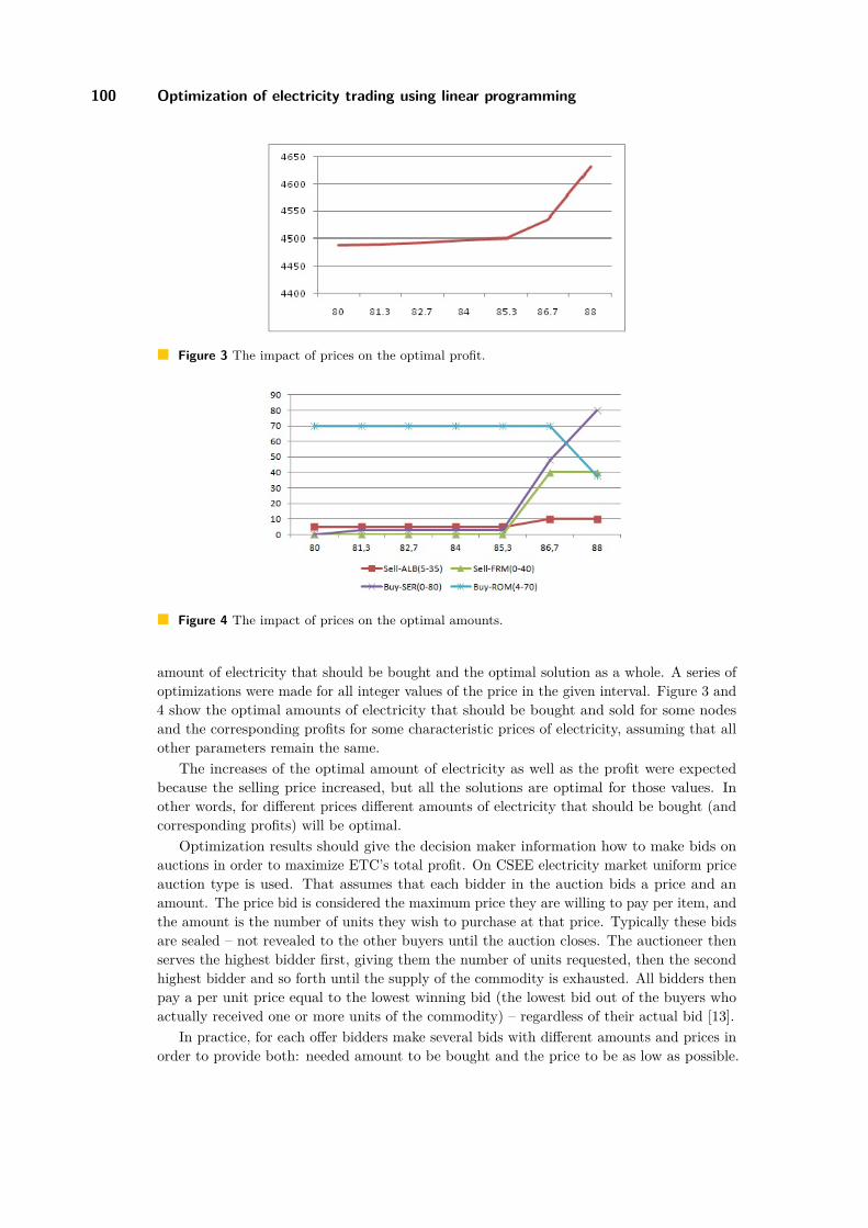
100 Optimization of electricity trading using linear programming
Figure 3 The impact of prices on the optimal profit.
Figure 4 The impact of prices on the optimal amounts.
amount of electricity that should be bought and the optimal solution as a whole. A series ofoptimizations were made for all integer values of the price in the given interval. Figure 3 and4 show the optimal amounts of electricity that should be bought and sold for some nodesand the corresponding profits for some characteristic prices of electricity, assuming that allother parameters remain the same.
The increases of the optimal amount of electricity as well as the profit were expectedbecause the selling price increased, but all the solutions are optimal for those values. Inother words, for different prices different amounts of electricity that should be bought (andcorresponding profits) will be optimal.
Optimization results should give the decision maker information how to make bids onauctions in order to maximize ETC’s total profit. On CSEE electricity market uniform priceauction type is used. That assumes that each bidder in the auction bids a price and anamount. The price bid is considered the maximum price they are willing to pay per item, andthe amount is the number of units they wish to purchase at that price. Typically these bidsare sealed – not revealed to the other buyers until the auction closes. The auctioneer thenserves the highest bidder first, giving them the number of units requested, then the secondhighest bidder and so forth until the supply of the commodity is exhausted. All bidders thenpay a per unit price equal to the lowest winning bid (the lowest bid out of the buyers whoactually received one or more units of the commodity) – regardless of their actual bid [13].
In practice, for each offer bidders make several bids with different amounts and prices inorder to provide both: needed amount to be bought and the price to be as low as possible.

M.R. Marinović, D.D. Makajić-Nikolić, M.J. Stanojević, and L.S. Ðorđević 101
Table 2 List of bids derived from optimal solutions.
Bids Amountsof el.
Price Accumulatedamount
Guaranteedprofit
B1 3 481.3-85.3 3 4489-4501B2 45 85.4-86.7 48 4535B3 35 86.8-88 80 4631
On the basis of the presented optimal solutions we can suggest the ETC decision maker tomake bids as presented in Table 2.Depending on the price equal to the lowest winning bid (which will not be known till theend of the auction), ETC will buy 0, 3, 48 or 80 MWh from node SER. For prices that arepresented as intervals in Table 2, ETC decision maker can give any price from that intervalfor which it estimates that can win. Anyhow, the corresponding amount will be optimal. Theprofits given in the rightmost column represent the optimal profit in case that correspondingbid becomes the lowest winning bid. If any lower bid wins, the profit will be bigger.
5 Conclusions
In this paper, problem of day-ahead energy planning in the Energy Trading Companies havebeen considered. It has been formulated as a linear programming problem. Day-ahead energyplanning implies finding the optimal amounts of electricity that should be bought from eachsupplier and sold to each buyer and the optimal routes which can satisfy the daily demandsusing the purchased and additional energy transmission capacities.
A real numerical example was considered and demonstrate the usage of the model whichhas been presented in this paper. Since the developed model is linear, it can be used to solvereal life problems of large dimensions.
As a topic of further research, the trading through futures markets can be taken intoconsideration. Another topic of future research is modeling long term planning strategy ofEnergy Trading Companies.
References1 EFET, Electricity markets harmonisation – New edition. http://www.efet.org2 GLPK, GNU Linear Programming Kit. http://www.gnu.org/s/glpk/3 HARCOURT, Harcourt strategy sheet – Energy and Power Trading. http://www.
harcourt.ch4 Hsieh C. C., Chen Y. T. Resource allocation decisions under various demands and cost
requirements in an unreliable flow network. Comput Oper Res 32:2771–2784, 2005.5 Kristiansen T. An assessment of the Danish–German cross-border auctions. Energy Policy
35:3369–3382, 2007.6 Liu M., Wu F. F. Portfolio optimization in electricity markets. Electr Pow Syst Res 77:1000–
1009, 2007.7 Nowak M. P., Schultz R. D., Westphalenm M. A. Stochastic Integer Programming Model
for Incorporating Day-Ahead Trading of Electricity into Hydro-Thermal Unit Commitment.Optim Eng 6:163–176, 2005.
8 Oggioni G., Smeers Y. Evaluating the impact of average cost based contracts on theindustrial sector in the European emission trading scheme. Cent Europ J Oper Re 17,2:181–217, 2009.
SCOR’12

102 Optimization of electricity trading using linear programming
9 Purchala K., Haesen E., Meeus L., Belmans R. Zonal network model of European intercon-nected electricity network, CIGRE/IEEE PES, International Symposium New Orleans, pp.362–369, 2005.
10 Quelhas A., Gil E., McCalley J. D., Ryan S. M. A Multiperiod Generalized Network FlowModel of the U.S. Integrated Energy System: Part I–Model Description. IEEE T PowerSyst 22, 2:829–836, 2007.
11 Thery R., Zarate P. Energy planning: a multi-level and multicriteria decision makingstructure proposal. Cent Europ J Oper Re 17, 3:265–274, 2009.
12 Triki C., Beraldi P., Gross G. Optimal capacity allocation in multi-auction electricity mar-kets under uncertainty. Comput Oper Res 32:201–217, 2005.
13 Vijay K., Auction theory. Academic Press, San Diego, 2002.

A Bilevel Mixed Integer Linear ProgrammingModel for Valves Location in Water DistributionSystemsAndrea Peano, Maddalena Nonato, Marco Gavanelli, StefanoAlvisi, and Marco Franchini
Department of Engineering,University of FerraraVia Saragat, 144122, Ferrara, Italy{andrea·peano, maddalena·nonato, marco·gavanelli, stefano·alvisi,marco·franchini}@unife·it
AbstractThe positioning of valves on the pipes of a Water Distribution System (WDS) is a core decision inthe design of the isolation system of a WDS. When closed, valves permit to isolate a small portionof the network, so called a sector, which can be de-watered for maintenance purposes at the costof a supply disruption. However, valves have a cost so their number is limited, and their positionmust be chosen carefully in order to minimize the worst-case supply disruption which may occurduring pipe maintenance. Supply disruption is usually measured as the undelivered user demand.When a sector is isolated by closing its boundary valves, other portions of the network maybecome disconnected from the reservoirs as a secondary effect, and experience supply disruptionas well. This induced isolation must be taken into account when computing the undelivereddemand induced by a sector isolation. While sector topology can be described in terms of graphpartitioning, accounting for induced undelivered demand requires network flow modeling. Theaim of the problem is to locate a given number of valves at the extremes of the network pipes sothat the maximum supply disruption is minimized. We present a Bilevel Mixed Integer LinearProgramming (MILP) model for this problem and show how to reduce it to a single level MILPby exploiting duality. Computational results on a real case study are presented, showing theeffectiveness of the approach.
1998 ACM Subject Classification G.1.6 Optimization
Keywords and phrases Isolation Valves Positioning, Bilevel Programming, Hydroinformatics
Digital Object Identifier 10.4230/OASIcs.SCOR.2012.103
1 Introduction
In this Section we introduce a real problem in hydraulic engineering concerning the locationof the isolation valves of a Water Distribution System, and reformulate it as a graph basedoptimization problem. A mathematical model is presented in Section 2, computational resultsare presented in Section 3 where conclusions are drawn.
1.1 Valves closure and sector isolationWater Distribution Systems (WDSs) are complex systems whose mission is to supply waterto the communities living in their service area. A WDS is made of several components, themain ones being: a set of reservoirs feeding the WDS, a set of pipes delivering water to the
© Andrea Peano, Maddalena Nonato, Marco Gavanelli, Stefano Alvisi, and Marco Franchini;licensed under Creative Commons License NC-ND
3rd Student Conference on Operational Research (SCOR 2012).Editors: Stefan Ravizza and Penny Holborn; pp. 103–112
OpenAccess Series in InformaticsSchloss Dagstuhl – Leibniz-Zentrum für Informatik, Dagstuhl Publishing, Germany
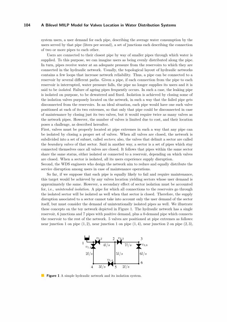
104 A Bilevel MILP Model for Valves Location in Water Distribution Systems
system users, a user demand for each pipe, describing the average water consumption by theusers served by that pipe (liters per second), a set of junctions each describing the connectionof two or more pipes to each other.
Users are connected to their closest pipe by way of smaller pipes through which water issupplied. To this purpose, we can imagine users as being evenly distributed along the pipe.In turn, pipes receive water at an adequate pressure from the reservoirs to which they areconnected in the hydraulic network. Usually, the topological layout of hydraulic networkscontains a few loops that increase network reliability. Thus, a pipe can be connected to areservoir by several different paths. Given a pipe, if each connection from the pipe to eachreservoir is interrupted, water pressure falls, the pipe no longer supplies its users and it issaid to be isolated. Failure of ageing pipes frequently occurs. In such a case, the leaking pipeis isolated on purpose, to be dewatered and fixed. Isolation is achieved by closing some ofthe isolation valves purposely located on the network, in such a way that the failed pipe getsdisconnected from the reservoirs. In an ideal situation, each pipe would have one such valvepositioned at each of its two extremes, so that only that pipe could be disconnected in caseof maintenance by closing just its two valves, but it would require twice as many valves asthe network pipes. However, the number of valves is limited due to cost, and their locationposes a challenge, as described hereafter.First, valves must be properly located at pipe extremes in such a way that any pipe canbe isolated by closing a proper set of valves. When all valves are closed, the network issubdivided into a set of subnet, called sectors; also, the valves that delimit a sector are calledthe boundary valves of that sector. Said in another way, a sector is a set of pipes which stayconnected themselves once all valves are closed. It follows that pipes within the same sectorshare the same status, either isolated or connected to a reservoir, depending on which valvesare closed. When a sector is isolated, all its users experience supply disruption.Second, the WDS engineers who design the network aim to reduce and equally distribute theservice disruption among users in case of maintenance operations.
So far, if we suppose that each pipe is equally likely to fail and require maintenance,this target would be achieved by any valves location yielding sectors whose user demand isapproximately the same. However, a secondary effect of sector isolation must be accountedfor, i.e., unintended isolation. A pipe for which all connections to the reservoirs go throughthe isolated sector will be isolated as well when that sector is closed. Therefore, the supplydisruption associated to a sector cannot take into account only the user demand of the sectoritself, but must consider the demand of unintentionally isolated pipes as well. We illustratethese concepts on the toy network depicted in Figure 1. The hydraulic network has a singlereservoir, 6 junctions and 7 pipes with positive demand, plus a 0-demand pipe which connectsthe reservoir to the rest of the network. 5 valves are positioned at pipe extremes as follows:near junction 1 on pipe (1, 2), near junction 1 on pipe (1, 4), near junction 2 on pipe (2, 3),
b b b
b b b
12 3
4 56
v3,6
v2,3
v5,4
v1,2
v1,4
2l/s
4l/s 7l/s
5l/s 6l/s
3l/s 2l/s
Figure 1 A simple hydraulic network and its isolation system.
A. Peano, M. Nonato, M. Gavanelli, S. Alvisi, and M. Franchini 105
near junction 3 on pipe (3, 6), and finally near junction 5 on pipe (4, 5). Three sectors areinduced by those valves, namely S1 made of pipes (1, 4), (4, 5) with demand 5l/s; S2 made ofpipes (1, 2), (2, 5), (5, 6), (3, 6) with demand 17l/s; S3 made of pipe (2, 3) with demand 7l/s.Let vi,j denote a valve located on pipe (i, j) near i, and let vj,i be the one close to j. If pipe(2, 3) needs repairing, valves v1,2 and v3,6 can be closed, with a supply disruption of 7l/s. Ifpipe (5, 6) leaks, the boundary valves of S2 will be closed, namely v1,2, v5,4, v3,6, and v2,3,but the supply disruption will be 24 = 17 + 7, greater than its sector demand, accounting forthe unintended isolation of S3.
The Isolation System Design (ISD) of WDSs consists of locating a limited number of valvesat pipe extremes so that any pipe can be isolated. What an optimal placement is may dependon several criteria that give rise to different objective functions; in particular, the BottleneckIsolation Valves Location Problem (BIVLP) minimizes the maximum undelivered demand.The two main issues related to the ISD problem addressed in the hydraulic engineeringliterature, are: the identification of the segments and unintended isolation due to the closureof some isolation valves, and the optimal location of isolation valves. Regarding the first topic,among others, [12, 13] exploit a dual representation of the network, with segments treatedas nodes and valves as links; [5, 9] exploit the topological incidence matrices to identify thesegments. Regarding the second topic, both [9] and [5] tackle the problem by bi-objectivegenetic algorithms, seeking a compromise between cost and solution quality. In particular,the former minimizes the number of valves and the maximum supply disruption. The latterminimizes the cost of the installed valves related to pipe diameters and the average supplydisruption weighted by the probability of pipe failure. Both provide an approximation of thePareto frontier and no bounds to evaluate the quality of the heuristic solutions.
The only two exact approaches for the BIVLP we are aware of are provided in [2] and [7],which apply two different tools of the Logic Programming field to minimize the maximumundelivered demand given a fixed number of valves. The former is based on Constraint LogicProgramming on Finite Domain [11] (CLP(FD)), and models the problem as a two-playersgame and three moves: player 1 locates the valves, player 2 chooses a pipe to break, andplayer 1 closes a set of valves. The latter is based on the Answer Set Programming [8] (ASP)paradigm and uses the concept of “extended sector”, that is the union of a sector with its(if existing) unintended isolations. Both can be used to compute the Pareto frontier of theproblem tackled by [9] by solving a sequence of instances with an increasing number ofvalves. Different models for the BIVLP have been proposed in each paper, with different prosand cons regarding prototyping and computing times. At present the best computationalperformance is achieved by the CLP(FD) model [2], which implements a redundant valveselimination technique and bounding procedures, and which is our benchmark.
In the following we reformulate the BIVLP in the framework of graph theory, and set thebasis for the mathematical optimization model provided in Section 2.
1.2 Hydraulic sectors and graph partitioningThe Graph Partitioning problem (GPP) is one of the most studied problems in combinatorialoptimization, and admits several variants. Recall that a partition of a set is a collection ofnon-empty disjoint subsets whose union returns the set. Generally speaking, GPP consistsof partitioning the vertices of a graph into a set of connected components by removinga minimum (weight) set of edges, according to some criteria. For example, the numberof components of the partition is fixed, and the number of nodes in each component isbounded from above. The set of removed edges is usually referred to as a multicut. Literaturereferences are many, among which [3] investigates the polytopes associated to the integer
SCOR’12

106 A Bilevel MILP Model for Valves Location in Water Distribution Systems
programming formulations of the major variants, and [6] studies the convex hull of incidencevectors of feasible multicuts for the capacitated GPP.
The several analogies between the hydraulic network sectorisation and graph partitioning,as recently exploited in the hydraulic engineering literature [14], seem at first to provide anideal framework for modelling BIVLP. Recall that each pipe must belong to one sector inorder to be isolated if required, but only one sector, due to the minimality of sector definition.Therefore, sectors induce a partition on the positive demand pipes, whose associated multicutmodels the location of the isolation valves at pipe extremes. This simple correspondence,though, does not allow us to address the issue of unintended isolation. To meet thisrequirement we need to introduce an extended graph that represents the topology of thenetwork, on which flow variables will model water flows, thus capturing unintended supplydisruption. We first provide a graph representation of the hydraulic network supporting graphpartition, and in the next Section we show how to extend such graph to handle unintendedisolation.
First, we suppose to concentrate the user demand of a pipe (i, j) at a single point denotedas εij , located in the middle of the pipe. Denote by δεij
such demand. Then, we shrink allthe reservoirs into a single one, to which we associate node σ. Now we can introduce theundirected graph G = (V,E) defined as follows.The vertex set V is made of the union of: Σ = {σ}, where σ is the super source modellingthe set of reservoirs; Ψ, being the union over all pipes of the demand points εij ; Γ, modellingthe junctions of the hydraulic network.The edge set E is made of: T , the set of the few structural edges corresponding to 0-demandpipes which connect σ to a vertex in Γ; we denote as Γ(Σ) ⊂ Γ the subset of the junctionnodes adjacent to a reservoir. F , made of a pair of edges (i, εij) and (j, εij) for each pipe(i, j) in the hydraulic network. Figure 2 shows how the two adjacent pipes of the hydraulicnetwork are modelled in graph G.
ǫ232 31(2, ǫ23)ǫ12
(3, ǫ23)(2, ǫ12)(1, ǫ12)1 2 3(1, 2) (2, 3)
Figure 2 Two adjacent pipes of the hydraulic network and their representation in G.
Each edge in F may host a valve, while edges in T do not. In real life WDSs, actually, aspecial valve is always present on each pipe in T in order to isolate the reservoir from thenetwork, if the reservoir needs maintenance. However, such a valve would never be closed forpipe maintenance purposes, so we disregard it here. Therefore, we assume that the edges inT bear no valves, and that these edges, the reservoirs and the nodes in Γ(Σ) do not belongto any sector. Furthermore, to keep notation simple, we suppose that all pipes other thanthose incident on the reservoirs have positive demand.
Let hmax be the number of available valves, and smax the maximum number of sectorsadmitted. Denote by ∆s, for s ∈ S = {1, .., smax}, the undelivered demand associated tosector s, and it is given by the sum of δεij
for each pipe (i, j) which gets isolated whenthe boundary valves of sector s are closed. Note that isolating a sector s on the hydraulicnetwork corresponds to the removal of all edges (i, εij) ∈ F on graph G such that a boundaryvalve of s is positioned on pipe (i, j) near junction i. We search for the location of at mosthmax valves on as many edges of F yielding at most smax sectors such that maxs∈S{∆s} isminimum. In Section 2 we provide a mathematical model for this problem.
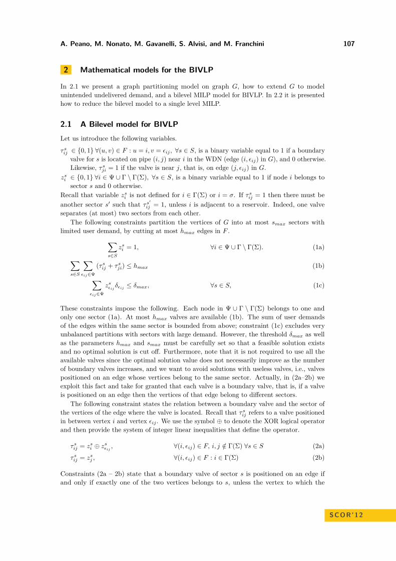
A. Peano, M. Nonato, M. Gavanelli, S. Alvisi, and M. Franchini 107
2 Mathematical models for the BIVLP
In 2.1 we present a graph partitioning model on graph G, how to extend G to modelunintended undelivered demand, and a bilevel MILP model for BIVLP. In 2.2 it is presentedhow to reduce the bilevel model to a single level MILP.
2.1 A Bilevel model for BIVLPLet us introduce the following variables.
τsij ∈ {0, 1} ∀(u, v) ∈ F : u = i, v = εij , ∀s ∈ S, is a binary variable equal to 1 if a boundaryvalve for s is located on pipe (i, j) near i in the WDN (edge (i, εij) in G), and 0 otherwise.Likewise, τsji = 1 if the valve is near j, that is, on edge (j, εij) in G.
zsi ∈ {0, 1} ∀i ∈ Ψ ∪ Γ \ Γ(Σ), ∀s ∈ S, is a binary variable equal to 1 if node i belongs tosector s and 0 otherwise.
Recall that variable zsi is not defined for i ∈ Γ(Σ) or i = σ. If τsij = 1 then there must beanother sector s′ such that τs′
ij = 1, unless i is adjacent to a reservoir. Indeed, one valveseparates (at most) two sectors from each other.
The following constraints partition the vertices of G into at most smax sectors withlimited user demand, by cutting at most hmax edges in F .∑
s∈Szsi = 1, ∀i ∈ Ψ ∪ Γ \ Γ(Σ). (1a)∑
s∈S
∑εij∈Ψ
(τsij + τsji) ≤ hmax (1b)
∑εij∈Ψ
zsεijδεij≤ δmax, ∀s ∈ S, (1c)
These constraints impose the following. Each node in Ψ ∪ Γ \ Γ(Σ) belongs to one andonly one sector (1a). At most hmax valves are available (1b). The sum of user demandsof the edges within the same sector is bounded from above; constraint (1c) excludes veryunbalanced partitions with sectors with large demand. However, the threshold δmax as wellas the parameters hmax and smax must be carefully set so that a feasible solution existsand no optimal solution is cut off. Furthermore, note that it is not required to use all theavailable valves since the optimal solution value does not necessarily improve as the numberof boundary valves increases, and we want to avoid solutions with useless valves, i.e., valvespositioned on an edge whose vertices belong to the same sector. Actually, in (2a–2b) weexploit this fact and take for granted that each valve is a boundary valve, that is, if a valveis positioned on an edge then the vertices of that edge belong to different sectors.
The following constraint states the relation between a boundary valve and the sector ofthe vertices of the edge where the valve is located. Recall that τsij refers to a valve positionedin between vertex i and vertex εij . We use the symbol ⊕ to denote the XOR logical operatorand then provide the system of integer linear inequalities that define the operator.
τsij = zsi ⊕ zsεij, ∀(i, εij) ∈ F, i, j /∈ Γ(Σ) ∀s ∈ S (2a)
τsij = zsj , ∀(i, εij) ∈ F : i ∈ Γ(Σ) (2b)
Constraints (2a – 2b) state that a boundary valve of sector s is positioned on an edge ifand only if exactly one of the two vertices belongs to s, unless the vertex to which the
SCOR’12
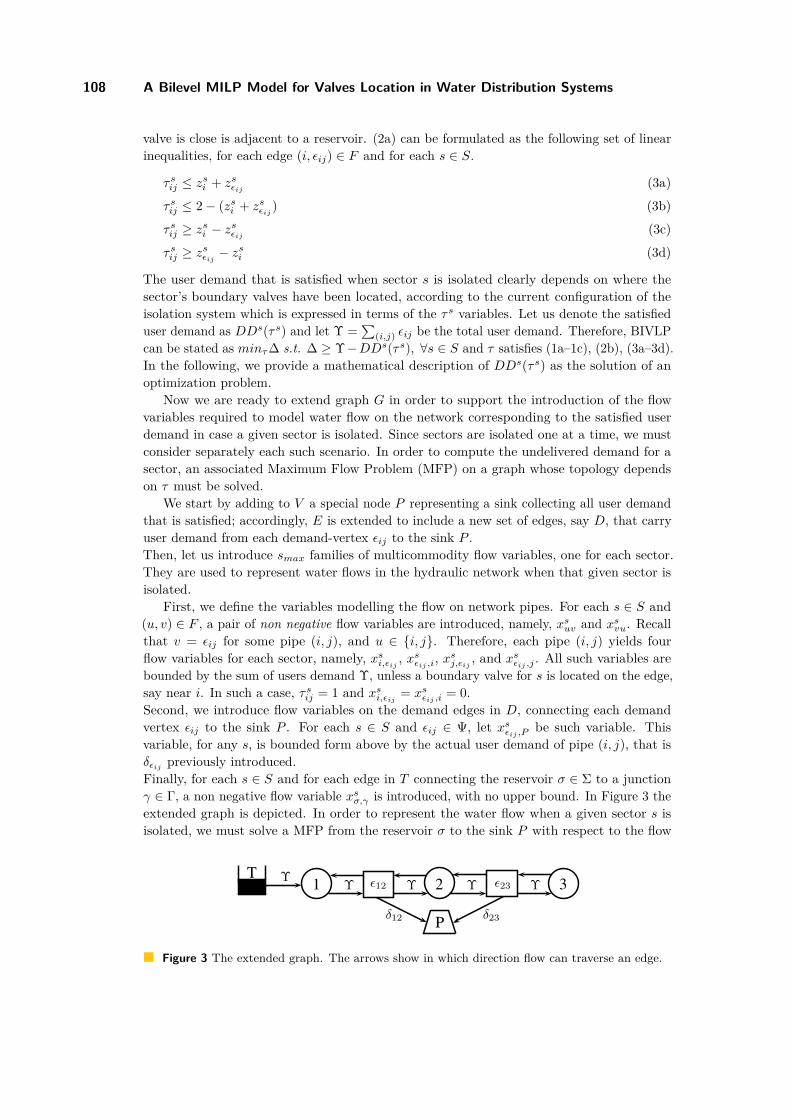
108 A Bilevel MILP Model for Valves Location in Water Distribution Systems
valve is close is adjacent to a reservoir. (2a) can be formulated as the following set of linearinequalities, for each edge (i, εij) ∈ F and for each s ∈ S.
τsij ≤ zsi + zsεij(3a)
τsij ≤ 2− (zsi + zsεij) (3b)
τsij ≥ zsi − zsεij(3c)
τsij ≥ zsεij− zsi (3d)
The user demand that is satisfied when sector s is isolated clearly depends on where thesector’s boundary valves have been located, according to the current configuration of theisolation system which is expressed in terms of the τs variables. Let us denote the satisfieduser demand as DDs(τs) and let Υ =
∑(i,j) εij be the total user demand. Therefore, BIVLP
can be stated as minτ∆ s.t. ∆ ≥ Υ−DDs(τs), ∀s ∈ S and τ satisfies (1a–1c), (2b), (3a–3d).In the following, we provide a mathematical description of DDs(τs) as the solution of anoptimization problem.
Now we are ready to extend graph G in order to support the introduction of the flowvariables required to model water flow on the network corresponding to the satisfied userdemand in case a given sector is isolated. Since sectors are isolated one at a time, we mustconsider separately each such scenario. In order to compute the undelivered demand for asector, an associated Maximum Flow Problem (MFP) on a graph whose topology dependson τ must be solved.
We start by adding to V a special node P representing a sink collecting all user demandthat is satisfied; accordingly, E is extended to include a new set of edges, say D, that carryuser demand from each demand-vertex εij to the sink P .Then, let us introduce smax families of multicommodity flow variables, one for each sector.They are used to represent water flows in the hydraulic network when that given sector isisolated.
First, we define the variables modelling the flow on network pipes. For each s ∈ S and(u, v) ∈ F , a pair of non negative flow variables are introduced, namely, xsuv and xsvu. Recallthat v = εij for some pipe (i, j), and u ∈ {i, j}. Therefore, each pipe (i, j) yields fourflow variables for each sector, namely, xsi,εij
, xsεij ,i, xsj,εij
, and xsεij ,j. All such variables are
bounded by the sum of users demand Υ, unless a boundary valve for s is located on the edge,say near i. In such a case, τsij = 1 and xsi,εij
= xsεij ,i= 0.
Second, we introduce flow variables on the demand edges in D, connecting each demandvertex εij to the sink P . For each s ∈ S and εij ∈ Ψ, let xsεij ,P
be such variable. Thisvariable, for any s, is bounded form above by the actual user demand of pipe (i, j), that isδεij previously introduced.Finally, for each s ∈ S and for each edge in T connecting the reservoir σ ∈ Σ to a junctionγ ∈ Γ, a non negative flow variable xsσ,γ is introduced, with no upper bound. In Figure 3 theextended graph is depicted. In order to represent the water flow when a given sector s isisolated, we must solve a MFP from the reservoir σ to the sink P with respect to the flow
ǫ232 31 ǫ12
P δ23δ12
Υ Υ Υ ΥT Υ
Figure 3 The extended graph. The arrows show in which direction flow can traverse an edge.
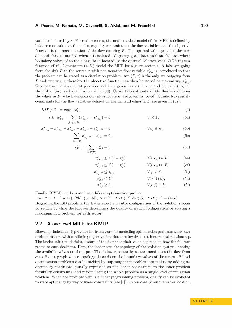
A. Peano, M. Nonato, M. Gavanelli, S. Alvisi, and M. Franchini 109
variables indexed by s. For each sector s, the mathematical model of the MFP is defined bybalance constraints at the nodes, capacity constraints on the flow variables, and the objectivefunction is the maximization of the flow entering P . The optimal value provides the userdemand that is satisfied when s is isolated. Capacity goes down to 0 on the arcs whereboundary valves of sector s have been located, so the optimal solution value DDs(τs) is afunction of τs. Constraints (4–5i) model the MFP for a given sector s. A fake arc goingfrom the sink P to the source σ with non negative flow variable xsPσ is introduced so thatthe problem can be stated as a circulation problem. Arc (P, σ) is the only arc outgoing fromP and entering σ, therefore the objective function can then be stated as maximizing xsP,σ.Zero balance constraints at junction nodes are given in (5a), at demand nodes in (5b), atthe sink in (5c), and at the reservoir in (5d). Capacity constraints for the flow variables onthe edges in F , which depends on valves location, are given in (5e-5f). Similarly, capacityconstraints for the flow variables defined on the demand edges in D are given in (5g).
DDs(τs) = max xsP,σ (4)
s.t. xsσ,i +∑
j:εij∈Ψ(xsεij ,i − x
si,εij
) = 0 ∀i ∈ Γ, (5a)
xsi,εij+ xsj,εij
− xsεij ,i − xsεij ,j − x
sεij ,P = 0 ∀εij ∈ Ψ, (5b)∑
εij∈Ψxsεij ,P − x
sP,σ = 0, (5c)
xsP,σ −∑
i∈Γ(Σ)
xsσ,i = 0, (5d)
xsi,εij≤ Υ(1− τsij) ∀(i, εij) ∈ F, (5e)
xsεij ,i ≤ Υ(1− τsij) ∀(i, εij) ∈ F, (5f)
xsεij ,P ≤ δεij ∀εij ∈ Ψ, (5g)
xsσ,i ≤ Υ ∀i ∈ Γ(Σ), (5h)xsi,j ≥ 0, ∀(i, j) ∈ E. (5i)
Finally, BIVLP can be stated as a bilevel optimization problem.minτ∆ s. t. (1a–1c), (2b), (3a–3d), ∆ ≥ Υ−DDs(τs) ∀s ∈ S, DDs(τs) = (4-5i).Regarding the ISD problem, the leader select a feasible configuration of the isolation systemby setting τ , while the follower determines the quality of a such configuration by solving amaximum flow problem for each sector.
2.2 A one level MILP for BIVLPBilevel optimization [4] provides the framework for modelling optimization problems where twodecision makers with conflicting objective functions are involved in a hierarchical relationship.The leader takes its decisions aware of the fact that their value depends on how the followerreacts to such decisions. Here, the leader sets the topology of the isolation system, locatingthe available valves on the pipes. The follower, sector by sector, maximizes the flow fromσ to P on a graph whose topology depends on the boundary valves of the sector. Bileveloptimization problems can be tackled by imposing inner problem optimality by adding itsoptimality conditions, usually expressed as non linear constraints, to the inner problemfeasibility constraints, and reformulating the whole problem as a single level optimizationproblem. When the inner problem is a linear programming problem, duality can be exploitedto state optimality by way of linear constraints (see [1]). In our case, given the valves location,
SCOR’12
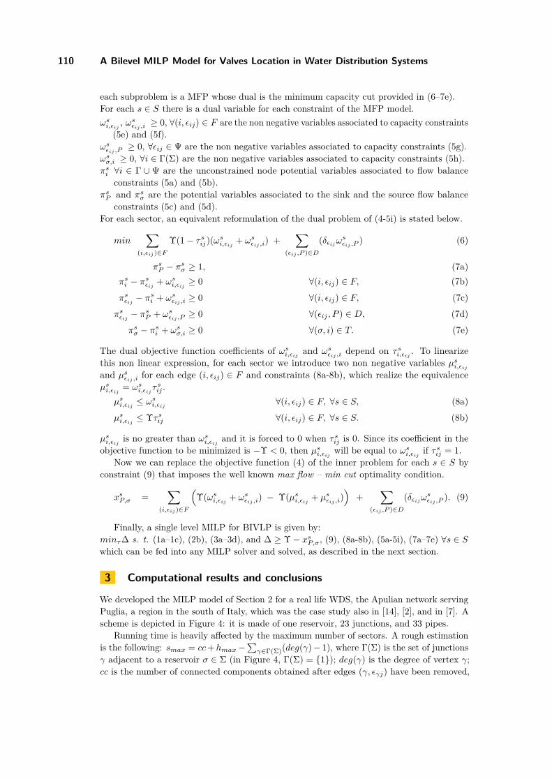
110 A Bilevel MILP Model for Valves Location in Water Distribution Systems
each subproblem is a MFP whose dual is the minimum capacity cut provided in (6–7e).For each s ∈ S there is a dual variable for each constraint of the MFP model.ωsi,εij
, ωsεij ,i≥ 0, ∀(i, εij) ∈ F are the non negative variables associated to capacity constraints
(5e) and (5f).ωsεij ,P
≥ 0, ∀εij ∈ Ψ are the non negative variables associated to capacity constraints (5g).ωsσ,i ≥ 0, ∀i ∈ Γ(Σ) are the non negative variables associated to capacity constraints (5h).πsi ∀i ∈ Γ ∪ Ψ are the unconstrained node potential variables associated to flow balance
constraints (5a) and (5b).πsP and πsσ are the potential variables associated to the sink and the source flow balance
constraints (5c) and (5d).For each sector, an equivalent reformulation of the dual problem of (4-5i) is stated below.
min∑
(i,εij)∈F
Υ(1− τsij)(ωsi,εij+ ωsεij ,i) +
∑(εij ,P )∈D
(δεijωsεij ,P ) (6)
πsP − πsσ ≥ 1, (7a)πsi − πsεij
+ ωsi,εij≥ 0 ∀(i, εij) ∈ F, (7b)
πsεij− πsi + ωsεij ,i ≥ 0 ∀(i, εij) ∈ F, (7c)
πsεij− πsP + ωsεij ,P ≥ 0 ∀(εij , P ) ∈ D, (7d)
πsσ − πsi + ωsσ,i ≥ 0 ∀(σ, i) ∈ T. (7e)
The dual objective function coefficients of ωsi,εijand ωsεij ,i
depend on τsi,εij. To linearize
this non linear expression, for each sector we introduce two non negative variables µsi,εij
and µsεij ,ifor each edge (i, εij) ∈ F and constraints (8a-8b), which realize the equivalence
µsi,εij= ωsi,εij
τsij .µsi,εij
≤ ωsi,εij∀(i, εij) ∈ F, ∀s ∈ S, (8a)
µsi,εij≤ Υτsij ∀(i, εij) ∈ F, ∀s ∈ S. (8b)
µsi,εijis no greater than ωsi,εij
and it is forced to 0 when τsij is 0. Since its coefficient in theobjective function to be minimized is −Υ < 0, then µsi,εij
will be equal to ωsi,εijif τsij = 1.
Now we can replace the objective function (4) of the inner problem for each s ∈ S byconstraint (9) that imposes the well known max flow – min cut optimality condition.
xsP,σ =∑
(i,εij)∈F
(Υ(ωsi,εij
+ ωsεij ,i) − Υ(µsi,εij+ µsεij ,i)
)+
∑(εij ,P )∈D
(δεijωsεij ,P ). (9)
Finally, a single level MILP for BIVLP is given by:minτ∆ s. t. (1a–1c), (2b), (3a–3d), and ∆ ≥ Υ− xsP,σ, (9), (8a-8b), (5a-5i), (7a–7e) ∀s ∈ Swhich can be fed into any MILP solver and solved, as described in the next section.
3 Computational results and conclusions
We developed the MILP model of Section 2 for a real life WDS, the Apulian network servingPuglia, a region in the south of Italy, which was the case study also in [14], [2], and in [7]. Ascheme is depicted in Figure 4: it is made of one reservoir, 23 junctions, and 33 pipes.
Running time is heavily affected by the maximum number of sectors. A rough estimationis the following: smax = cc+hmax−
∑γ∈Γ(Σ)(deg(γ)− 1), where Γ(Σ) is the set of junctions
γ adjacent to a reservoir σ ∈ Σ (in Figure 4, Γ(Σ) = {1}); deg(γ) is the degree of vertex γ;cc is the number of connected components obtained after edges (γ, εγj) have been removed,
A. Peano, M. Nonato, M. Gavanelli, S. Alvisi, and M. Franchini 111
bb
b
b
b
bb
b b
b
b
b
b
bb
b
b
b b
b
b
bb
1
239
10
13
22
12
114
6
519
1817
23
21
20148
715
16
T
Figure 4 The Apulian network.
for each junction γ ∈ Γ(Σ), except for the component made of σ, γ, and pipe (σ, γ). Anypipe with positive demand and incident on a junction in Γ(Σ) must have a valve locatednear the junction to be isolated. Once such valves have been placed, yielding cc sectors, atmost one more sector may result from the placement of one additional valve. This boundcan be tight for very sparse networks, such as a tree, but real WDSs have several loops. Atighter estimate for smax and a downsizing of the MILP model can be achieved by moresophisticated procedures exploiting the network topology of the instance, and are currentlyunder investigation.
As in [2], hmax varies in [5, · · · , 14] and the time limit for each instance is 8000 seconds.In the Apulian network cc = 1, Γ(Σ) = {1} and deg(1) = 4, then we have that smax =1 + hmax − (4− 1) = hmax − 2, hence smax varies in [3, · · · , 12].
The MILP solver is Gurobi Optimizer 4.6 [10], experiments were run on a Intel dual corearchitecture based on P8400 CPUs, 2.26 GHz, 4GB of RAM.
Figure 5 for each value of hmax reports the running time for the optimally solved instances,and the time the best feasible solution was found for the others. For such instances, labelsreport the gap between the best feasible MILP solution (zMILP ) and the optimal one providedin [2] (zCLP ). Note that for hmax = 8, 9, 14 we find the optimal solution within the timelimit but we cannot certify it.
In conclusion, we provided a third exact solution approach to the BIVLP, based on MILP.A first implementation outperforms the ASP based approach and can solve to optimality
3 4 5 6 7 8 9 10 11 12 13 140
1000
2000
3000
4000
5000
6000
7000
8000
0
1000
2000
3000
4000
5000
6000
7000
8000
MILP – Total computing timeMILP – Best feasible solution timeCLP(FD) – Total computing timeCLP(FD) – Best feasible solution time
# Valves
Co
mp
uti
ng
tim
e
0% 0% 3.6% 1.5% 10.3%
| zCLP – zMILP | / zCLP
0%
Figure 5 Computation time and solution gap values with different number of valves.
SCOR’12
112 A Bilevel MILP Model for Valves Location in Water Distribution Systems
several instances of those solved by the CLP(FD) based approach in the same time limit, whileprovides good quality solutions to the others. Regarding the Pareto front generation, someiterations could be saved w.r.t. [2] where the number of used valves is fixed. Current researchis devoted to improve the computational performance by: tuning the solver parameterswhich have been used at their default value; strengthening the GPP constraints takingadvantage of the literature studies on its polyhedral structure [3, 6]; reducing symmetries inthe model; tightening the estimate on smax exploiting the WDS’s graph topology; exploitingthe knowledge of the exact solution with one more (one less) available valve in the computationof the Pareto optimal frontier. Furthermore, we aim to tackle different objective functionsbuilding on the MILP model here presented to formulate the feasible region of the ISDproblem. For example, we plan to handle different probabilities of pipe failures and pipedependent valve costs. Finally, hybrid approaches integrating MILP and CLP will beexplored.
References1 M. Bruglieri, P. Cappanera, A. Colorni, and M. Nonato. Modeling the gateway location
problem for multicommodity flow rerouting. In J. Pahl et al., editor, Network Optimization,volume 6701 of Lecture Notes in Computer Science. Springer Berlin / Heidelberg, 2011.
2 M. Cattafi, M. Gavanelli, M. Nonato, S. Alvisi, and M. Franchini. Optimal placementof valves in a water distribution network with CLP(FD). Theory and Practice of LogicProgramming, 11(4-5):731–747, 2011.
3 S. Chopra and M. R. Rao. The partition problem. Mathematical Programming, 59(1), 1993.4 B. Colson, P. Marcotte, and G. Savard. An overview of bilevel optimization. Annals of
Operations Research, 153:235–256, 2007. 10.1007/s10479-007-0176-2.5 E. Creaco, M. Franchini, and S. Alvisi. Optimal placement of isolation valves in water
distribution systems based on valve cost and weighted average demand shortfall. Journalof Water Resources Planning and Management, 24(15), 2010.
6 C. Ferreira, A. Martin, C. de Souza, R. Weismantel, and L. Wolsey. Formulations and validinequalities for the node capacitated graph partitioning problem. Mathematical Program-ming, 74(3), 1996.
7 M. Gavanelli, M. Nonato, A. Peano, S. Alvisi, and M. Franchini. An ASP approach for thevalves positioning optimization in a water distribution system. In F. Lisi, editor, 9th ItalianConvention on Computational Logic (CILC 2012), Rome, Italy, volume 857 of CEUR Work-shop Proceedings, pages 134–148, 2012.
8 M. Gelfond. Answer sets. In Handbook of Knowledge Representation, chapter 7. Elsevier,2007.
9 O. Giustolisi and D. A. Savić. Identification of segments and optimal isolation valve systemdesign in water distribution networks. Urban Water Journal, 2010.
10 Gurobi Optimization, Inc. Gurobi optimizer reference manual. http://www.gurobi.com.11 J. Jaffar and M. J. Maher. Constraint logic programming: A survey. Journal of Logic
Programming, 19/20:503–581, 1994.12 H. Jun and G. V. Loganathan. Valve-controlled segments in water distribution systems.
Journal of Water Resources Planning and Management, 133(2), 2007.13 J.-J. Kao and P.-H. Li. A segment-based optimization model for water pipeline replacement.
J. Am. Water Works Assoc., 99(7):83–95, 2007.14 A. D. Nardo, M. D. Natale, G. Santonastaso, and S. Venticinque. Graph partitioning
for automatic sectorization of a water distribution system. In D. Savic, Z. Kapelan, andD. Butler, editors, Urban Water Management: Challenges and Opportunities, volume 3,pages 841–846. Centre for Water Systems, University of Exeter, Exeter (UK), 2011.

![Einsteingravityasa3Dconformallyinvarianttheory · arXiv:1010.2481v2 [gr-qc] 28 Mar 2011 Einsteingravityasa3Dconformallyinvarianttheory HenriqueGomes∗ UniversityofNottingham,SchoolofMathematicalSciences](https://img.pdfslide.net/doc/110x75/5fa5fc17f6e2a617f700a314/einsteingravityasa3dconformallyinvarianttheory-arxiv10102481v2-gr-qc-28-mar.jpg)