Embed Size (px)
Citation preview

From the SelectedWorks of Sanhita Athalye
2008
Drought Resilience in Agriculture: The Role ofTechnological Options, Land Use Dynamics andRisk PerceptionRam RanjanSanhita Athalye, Indian Institute of Technology - Kharagpur
Available at: https://works.bepress.com/sanhita_athalye/2/

Drought Resilience in Agriculture: The Role of Technological Options, Land Use Dynamics and Risk Perception
Ram Ranjan Economist, CSRIO Land and Water
Private Bag No. 5, Wembley WA 6913, Australia Ph: 61 8 93336145, email: [email protected]
and
Sanhita Athalye Indian Institute of Technology, Kharagpur
West Bengal, India 721302 Ph: 91 9732985223, email: [email protected]
Abstract
This paper explores the role of behavioural factors --such as subjective risk perception over the probability of droughts, of the probability of land getting urbanized and of resistance to revising beliefs over water scarcity situation, in determining farmers’ resilience to droughts. A measure of resilience in agriculture, in wake of severe and sustained droughts, is derived as the ability to continue farming, by saving and carrying forward water, through the adoption of water efficient technology. Findings indicate that behavioural factors dominate the decision to adopt when the economic factors, such as the price of water, do not capture the true opportunity costs of water. The range of available technological options is crucial too, as marginal improvements in technology do not lead to adoption. Empirical application to the case of lettuce farming in Western Australia reveals that in the presence of speculative benefits from land rezoning, technological adoption is done only for enhancing profits in agriculture, and not for improving resilience to droughts.
Keywords: drought resilience, risk perception, technology adoption, water scarcity, land rezoning, drought perception

2
1. Introduction
Farming all over world is facing pressure to use water efficiently due to its increasing
scarcity and rising urban and environmental water demands. When faced with the
prospect of long term water shortages in agriculture, farmers have the option to
mitigate water scarcity through investment in advanced technology options such as
drip irrigation, or to exit farming. Given these tough choices faced by the farmers,
their resilience to water shortages, particularly those borne out of sustained droughts,
is becoming an important policy question that has not yet been tackled adequately.
Resilience against severe droughts is an aspect that has not been fully explored
in the literature to the best of the authors’ knowledge1. Resilience to sustained
droughts could be enhanced through adoption of water saving technology. However,
several factors may influence technology adoption. These could be economic,
political, technological or behavioural. Farmer heterogeneity, which may lead to
differences in size, productivity or over risk perceptions, may play a key role in
deciding over who adopts and who exits. Climatic and policy related variations in
water supply are a crucial factor too, as they introduce uncertainty over returns from
such investments in technology. Sunk cost in new technology and the possibility of
speculative rewards from land rezoning, could also be determinants in investment
decisions. But the overall impact of each of these factors can be optimally evaluated
only when explored simultaneously.
There exists a considerable amount of literature on predicting the adoption of
technology in agriculture. However, most of the focus on technology adoption
decisions is placed upon the impact of such choices on short term profitability.
1 Keil et al. (2006) derive a measure of drought resilience based upon reduction in consumption of basic household necessities. This study is based upon ENSO related droughts in central Sulawesi, Indonesia.

3
Technology adoption could actually serve a bigger purpose for the farmers by
ensuring their ability to survive long drought periods, when water saved through the
better technology could be, either stored underground, or carried forward in future.
There is evidence in the literature over the influence of water shortages on
technology adoption decisions. For instance, drip irrigation technology even though it
was first introduced in California in 1969, did not pick until 1977-79. This coincided
with severe droughts in the region and higher oil prices (Carey and Zilberman 2000).
The impact of droughts on inducing technology adoption has also been studied by
Zilberman et al. (1995). Shuchk et al. (2005), using survey data for adoption of
efficient irrigation technology in drought affected regions of Colorado find that
drought indeed significantly improves the percentage of farms adopting modern
irrigation technologies, with the farmers having the most reliable sources of water as
the major adopters. A crucial question then is over how technology adoption decision
is influenced when the water savings resulting from such an adoption could be used
for enhancing resilience against sustained droughts.
The impact of water markets and stochastic water supply on technology
adoption has been studied by Carey and Zilberman (2002) and Dinar and Letey
(1991). Using the case of drip irrigation technology in California, they find that
farmers do not adopt the better technology unless the net present value from adoption
exceeds the costs by a large margin. They also argue that the presence of water
markets delay the adoption of water saving technology adoption as water could be
availed of through the market.
Most of the existing work on technology adoption so far is based upon the
option value approach made popular by Dixit and Pindyck (1994) and McDonald and
Seigel (1986). This basically argues that irreversibility associated with the investment

4
in sunk costs presents an option value for waiting and therefore delays waiting. These
studies include Khanna et al. (2000), Carey and Zilberman (2002), Isik (2001), etc.
However, while the option value approach derives an important insight into the timing
of adoption which is not captured by the net present value approach, there are several
other equally important factors that may influence technology adoption decisions by
farmers, which have not been adequately dealt with in the literature. These include
behavioural factors such as risk perception over droughts, opportunity for speculative
benefits from land rezoning, un-availability of economically viable technological
options and the political economy of agriculture. While Carey and Zilberman (2002)
find water markets as discouraging adoption in the US, in Australia the price of water
has been found to be too low to influence water saving technological choices in
Agriculture (Brennan 2008). Subjective perception of the probability of severe
droughts may vary amongst farmers and over time. Such considerations as well as the
possibility of reaping higher land prices from possible future urbanization make the
prediction of technology adoption a complex exercise.
In this paper we explore the nature of linkages between these previously
unexplored factors and their impact on farmers’ resilience to short term water
scarcity, severe droughts and pressure from Urbanization. The approach involves
modelling the ability to carry forward some or all of the water saved through better
technology which would have implications for surviving in the years when water
supply is severely constrained through droughts. This ability to save water for future
makes their survival in wake of a drought endogenous to their current decisions
related to water abstractions and technology adoption. The key results from this
analysis are that risk perception influences technology adoption choices thereby
determining their survival in agriculture, and that technological options that lead to

5
only marginal improvements in water saving are not adopted. Heterogeneity amongst
farmers matters as well. Their ability to revise expectations over future water scarcity
based upon current and past observations plays a crucial role in technology adoption,
however this could go either way based upon the realization of the current rainfall. A
farmer that does not revise his expectations of the mean rainfall based upon past and
current observations will always overestimate the mean rainfall in an approaching
drought scenario and therefore may not adopt the technology. Finally, land rezoning
possibilities further distort the choice over technology adoption and may make
farmers less resilient to droughts.
In what follows, we first lay out the analytical framework of the model of
technology adoption choices in the presence of a stochastic water supply, possibilities
of land urbanization (which yields positive rewards) and severe droughts and they
illustrate the intuition through an application to the case of lettuce farming in Western
Australia. Discussion and conclusion follow.
2. Model
The model considers a general farmer who has a single source of water which could
be rainfall, a reservoir he maintains, or an allocation from the government.
The stock dynamics of the reservoir follows the below equation:
(1) )())(1))((()()1( thdroughtPtraintreservoirtreservoir −−+=+
where )(train follows a normal distribution with mean µ & standard deviation σ
and )(th is the water harvested by the farmer in each time period. Harvesting is
optimally derived by the model. Further, P(drought) is the possibility of a per period
severe drought in the wake of which there is no water allocation to the farmer (or
there is no rainfall through which he could augment his reservoir) and the farmer has

6
to rely entirely on the stock of existing reservoir for farming as long as the drought
continues. Whenever such a drought happens, he is assumed to harvest a fixed water
quantity equal to “mets”, which may be the minimum evapotranspiration required for
producing crops. The ‘mets’ value is a proportion of optimum water application in a
normal year, which is essential to avoid damage to the crops. Table 2 below depicts
the mets value for fruits, Vegetables and other crops.
INSERT TABLE 2 HERE
Thus the reservoir in drought years takes the following path:
(2) metstresevoirtreservoirtreservoir −⋅−=+ )()()1( α Here, α is the proportional decrease in reservoir water due to evaporation, leakage,
etc. We further assume that there is no leakage from the reservoir in the wet years
without any loss of generality. Once the reservoir level goes below ‘mets’, the farmer
cannot sustain agriculture for another year and has to exit farming. The number of
consecutive years, ‘n(t)’, for which he can sustain in a severe drought depends on
several factors including his reservoir level at time t at which consecutive droughts
begin, on α and on mets. This value of n is crucial in determining the farmers survival
in agriculture and therefore could be construed as a measure of his resilience and is
derived by solving equation (2) for fixed amounts of harvesting (mets) until there is
less than ‘mets’ amount of water left in the reservoir as2:
(3) ( )
−
⋅+⋅+
=α
αα
1log
)(
)1(log
)(treservoirmets
mets
ceiltn
On exit from farming, he recovers some scrap value (‘scrap’) of land, equipment, etc.
2 This can be derived as shown in the appendix.

7
The farmer’s exit from farming could also be induced by another event: rezoning of
his farmland for urbanisation. Such a selling gives him greater rewards for the same
land (say U) as compared to a scrap value of land that he receives from selling it
before land is rezoned. The probability of land getting rezoned in any year ‘t’ is
assumed to be sigmoid, and is based upon the assumption that as population pressure
increases, agriculture areas near the periphery of urbanization get converted over
time.
(4) )()(
tb
taLP
+⋅=
Where parameters a and b determine the maximum value and the time at which the
probability of rezoning peaks. The profit function for the farmer in any normal year is
given as:
(5) )()()( tchftrainprofit h−⋅= π
Where π is the price of the agricultural produce and ch(t) is the cost of harvesting
water (or the price paid to the government for its allocation). In a severe drought
year, as ‘harvest = mets’, profit is defined as:
(6) )()()( tcmetsftfitdroughtpro h−⋅= π
The expected gain EG from farming in any year is thus:
(7) )())(1()( droughtPfitdroughtprodroughtPtrainprofitEG ⋅+−⋅=
Next let us consider the future output of a particular farmer starting from a
particular year. In order to obtain the total reward from farming, we break the
situation into several possible cases that are independent from each other. Consider
any particular year, say ‘T’, such that up to time period T the farmer does not exit, and

8
the exit situation starts after T. An exit situation for a farmer could arise due to
rezoning or consecutive droughts starting from year T+1. Hence, the probability of
this happening is :
(8)
)()())(1()( tndroughtPLPLP ⋅−+
Upto year T, the farmer obtains the expected gains from farming in each year.
Therefore the profit from agriculture upto year T is:
(9) }{})())(1()({)(
1
)( rtT
tG
tn edroughtPLPLPTagprofit E −
=
⋅⋅⋅−+= ∑
Upon exit rewards are either obtained due to exit from rezoning or losses from an n-
year drought followed by a scrap value of land and capital from exit in the year T+n.
Thus expected exit rewards are:
(10)
}])({})())(1()([{)(
)()(
1
)1)(()()1( ∑+
+=
−++−+− ⋅+⋅⋅⋅−++⋅⋅=tnT
Tt
rttnTrTnTr etfitdroughtproescrapdroughtPLPLPeULP
Texitprofit
The total profits (Eprofit) obtained from farming and exit, therefore are the sum of
equation (9) and (10) and given as:
(11)
∫∑
∑∞
+
+=
−++−
+−−
=
⋅+⋅⋅⋅−++
⋅⋅+⋅⋅⋅−+=
0)(
1
)1)(()(
)1(
1
)(
}])({})())(1()([{
)(}{})())(1()({
tnT
Tt
rttnTrTn
TrrtT
tG
tn
etfitdroughtproescrapdroughtPLPLP
eULPedroughtPLPLP
EprofitE

9
The farmer may have a choice to adopt a water saving technology which
reduces his water application rates and allows him to sustain through longer drought
periods. More efficient technologies may allow the farmer to survive through drought
periods by reducing water applications to minimum possible levels (Schuck et al.
2005). However, this comes at a sunk cost equal to the price of the new technology,
which is irreversible. Therefore, he is faced with a binary choice over whether or not
to adopt.
Let the cost of adoption be ‘ctech’ and the choice of adoption be 1 when
adopted and 0 when not adopted. The new rainprofit function is derived as3:
(12)
( )
)1()()((
)}()({
)()(})()({
)(1)(1()}()({
)(
−−=−⋅+
⋅⋅−−⋅+
−⋅−⋅−⋅=
txtxtxdotwhere
adoptionaftertchf
adoptionofyearfirstthefortxdottxctechtchf
adoptiontilltxdottxtchf
trainprofit
hnew
hnew
h
L
L
L
ππ
π
Similarly droughtprofit is obtained as:
(13)
( )
)1()()((
)}()({
)()(})()({
)(1)(1()}()({
)(
−−=−⋅+
⋅⋅−−⋅+
−⋅−⋅−⋅=
txtxtxdotwhere
adoptionaftertcmetsf
adoptionofyearfirstthefortxdottxctechtcmetsf
adoptiontilltxdottxtcmetsf
tfitdroughtpro
hnew
hnew
h
L
L
L
ππ
π
The above formulation so far does not consider the behavioral aspects of
decision making in agriculture when faced with severe droughts. The behavioral
element of our model is based on accumulated evidence in economics and psychology
literature (see summary in Hurley and Shogren, 2005). Assume that the farmer
assigns higher weights to low probabilities of droughts and lower weights to high 3
Technically, the farmer can dis-adopt, but numerically a constraint can be imposed upon the model to
disallow dis-adoption.

10
probabilities of droughts (also see Starmer, 2000 and Ranjan and Shogren 2007). Let
the weighting function follow an inverse S-shape. Following Prelec (1998), we use a
two-parameter weighting function as:
(14) γθ )ln()( pepw −−=
where θ is the parameter that primarily determines elevation, and γ is the parameter
that primarily determines curvature. Elevation reflects the inflection (reference) point
at which the farmer switches from overestimating low probability events to
underestimating high probability events, i.e., the degree of over- and underestimation;
curvature captures the idea that the farmer become less sensitive to changes in
probability the further they are from the inflection point (Tversky and Kahneman
1992; Gonzales and Wu 1999). Figure 1 below shows the subjective weighting of the
probability of droughts that converts an objective probability of once in 20 year
drought into a subjective probability of once in 10 years drought. The frequency of
droughts in Australia is roughly once in 18 years (Bureau of Meteorology 2008).
INSERT FIGURE 1 HERE
Further, so far we have assumed that per period additions to the reservoir,
either due to rainfall or due to allocation are being given by a distribution with a
certain mean and variance. However, when water scarcity is climate change related, it
is more likely that the mean rainfall (and therefore the water allocations) would be
downwardly adjusted over time. Rainfall is assumed to come from a distribution
whose mean gets adjusted over time as:
(15)
[ ] [ ])____(
_______
yrpriorwtmeanpriorwt
yrprioryrpriorwtmeanpriormeanpriorwtmeannew
+⋅+⋅=

11
Where prior_mean is the mean rainfall up to the penultimate year, wt_prior_mean is
weightage assigned to the mean rainfall up to the penultimate year, prior_yr is the
rainfall of preceding year and wt_prior_yr is the weightage assigned to rainfall of
preceding year. Given the above characterization of the farmer’s problem, his task is
to select optimal water allocation rate and decide over whether or not adopt the water
efficient technology in order to maximize his profits. Note that if rewards from land
rezoning are very high or the profits from farming very low (when the price of water
may become large), the farmer’s objective may not be to maximize his stay in
agriculture. His measure of resilience from droughts, as given by the parameter n,
may still indicate the length of drought that he can endure before exiting. In order to
further explore how these different aspects influence his decision making, we perform
an empirical illustration of the above analytical model that best fits the above
characterization. We pick the case of lettuce farmers in Western Australia who are
faced with the prospect of water curtailment in future due to decreasing groundwater
levels and increasing water demand from the urban and environmental sectors.
3. Empirical Illustration
We consider a lettuce farmer in Western Australia who may be faced with water
restrictions in future. Currently, most of the water in Western Australia is derived
from the Gnangara mound, which is a large underground reservoir for water (Dept. of
Environment 2005). Historically, the mound was considered as an unlimited source
for water, but with increasing frequency of droughts, the levels have been going
down. The city of Perth in Western Australia is the largest consumer of this
underground water and has been making increasing demands on its resources from a

12
mining boom related population explosion. Current policy options for mitigating
water scarcity involve metering water use in agriculture and curtailing its allocation to
farmers (Brennan 2007).
Given this brief background, assume that the farmer receives an annual water
allocation from the government a proportion, ‘β’, of which he can carry over to the
next year if unused in the current year. Assuming he has no other sources of water, his
water reservoir stock would evolve as:
(16) )()()()1( thtallocationrainadjtreservoirtreservoir −⋅+⋅=+ β
where rainadj is a curtailment from his current allocation. It is assumed that
government does not allocate any water during a drought year. The chance of such a
drought is 1 in 18 years (BOM 2008). However, for our empirical estimation we take
it to be once in 20 years for convenience. Water allocation is based upon the realized
rainfall in each year. For instance, if rainfall is 600 mm, it amounts to 6 ML of water
per hectare for the farmer. Figure 2 below depicts the rainfall in the past 18 years
which has a mean and variance of 8.038 and 1.0082 respectively.
INSERT IFGURE 2 HERE
Lettuce farming gross margin function is based upon Brennan (2007) and is
derived as:
(17) )h(t)-(+)(exp(-h(t)) -exp(--( 2⋅− δϕτεςκηϑχ th
Where harvesting of water for farming is in Mega Litres (ML) and
δϕτεςκηϑχ &,,,,,,, are parameters of the production function and are presented in
Table 3 below. This function is inclusive of the cost of water which are $50/ML.
INSERT TABLE 3 HERE

13
The term )h(t)-( 2⋅δϕτ ensures that productivity declines after water application
exceeds a certain optimal level. This decline in productivity assumption is consistent
with the empirical evidence in lettuce farming which is caused by nitrogen leaching.
The gross revenue function using the two sprinkler irrigation technologies are
presented in figure 3 below.
INSERT FIGURE 3 HERE
Sprinklers with 60% and 90% distribution uniformity (DU) are considered as two
technological choices, though intermediary uniformity is also possible. Increase in the
distribution uniformity makes for more efficient use of water. The farmer is taken to
have 60% uniformity for the base case. The technology with 90% distribution
uniformity comes at a cost of about $8,165/hectare, which once invested may not be
reverted back too.
3. 1. Scenarios In the base case scenario we assume that the farmer has a prediction over future water
supply which is based upon the mean and variance of past 18 years rainfall. This data
is shown in Figure 2 below. The predictions are generated using a random number
generator in GAMS for the mean and variances based upon the empirical observation.
Short term forecasts play a relatively minor role in the decision making of farmers as
compared to medium and long term forecasts (Perkins 2003). Therefore, pattern
generated by the random predictions could be considered as one possible long term
scenario under consideration by the farmer while he derives his long term
optimization path. The farmer revises his expectation over the mean rainfall in each
period as given by equation (15) above. In the base case the farmer does not adopt the
water saving technology as there is enough rainfall in each year. The years in which
technology is adopted are presented in Table 4 in the Appendix. Note also that we

14
restrict the reservoir capacity (or carry forward capacity) to 5 ML of water. The
number of years that he could survive in the wake of a severe drought , as given by n,
goes to zero right after the first year. This indicates that the farmer stays in farming
only dependent upon the rainfall and will be out of farming as soon as the drought
period starts. The expected profits from being in agriculture summed up to time t (as
given by the variable agprofit) are shown in figure 4 below.
INSERT FIGURE 4 HERE
Water abstraction, rainfall and the reservoir levels are depicted in figure 5 below.
INSERT FIGURE 5 HERE
In the first scenario we lower the mean rainfall to 6.038 from 8.038 in order to
observe the impact of a future expectation of reduced rainfall on farmer’s decision.
The farmer adopts the technology in year 48. However, when the parameter c of the
gross revenue function with 90 percent distribution uniformity is changed to 3.3,
adoption happens much earlier—in time period 20. This highlights the role of
availability of technological choices in influencing technology adoption. Marginal
improvements in technology discourage adoption as the costs of adoption are too high
and can only be profitably incurred when adoption happens too far in future—when
its discounted cost is lower.
In the second scenario, we consider the impact of a farmer’s subjective risk
perceptions on the probability of severe droughts in future. The base case has one in
twenty year chance of severe drought. However, the subjective weighing of the risks
increases this chance to 0.11, i.e. one in 10 years. The impact of this weighing is that
technology adoption happens much earlier, in year 34.
In the third scenario, we consider the impact of a higher land rezoning
possibility on technology adoption keeping mean rain low at 6.038. This is achieved
15
by raising the parameter a to 0.8 which increases the upper bound of maximum
probability to 0.8. Surprisingly, this case leads to adoption in year 48, similar to the
base case. This happens due the exogenous nature of risk of rezoning and the
associated positive rewards from rezoning which do not encourage water saving. It is
however possible that when urbanization comes at a cost, water saving options are
encouraged. This result is consistent with earlier finding in the literature, called
"impermanence syndrome" (for instance, Lockeretz 1989), that attributes inefficient
farming to speculative rewards from land rezoning.
INSERT FIGURE 6 HERE
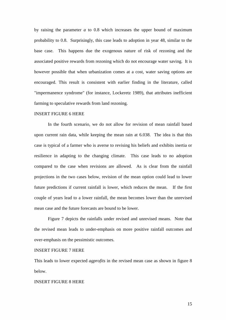
In the fourth scenario, we do not allow for revision of mean rainfall based
upon current rain data, while keeping the mean rain at 6.038. The idea is that this
case is typical of a farmer who is averse to revising his beliefs and exhibits inertia or
resilience in adapting to the changing climate. This case leads to no adoption
compared to the case when revisions are allowed. As is clear from the rainfall
projections in the two cases below, revision of the mean option could lead to lower
future predictions if current rainfall is lower, which reduces the mean. If the first
couple of years lead to a lower rainfall, the mean becomes lower than the unrevised
mean case and the future forecasts are bound to be lower.
Figure 7 depicts the rainfalls under revised and unrevised means. Note that
the revised mean leads to under-emphasis on more positive rainfall outcomes and
over-emphasis on the pessimistic outcomes.
INSERT FIGURE 7 HERE
This leads to lower expected agprofits in the revised mean case as shown in figure 8
below.
INSERT FIGURE 8 HERE

16
However, if the first couple of years lead to a higher rainfall, the opposite may happen
too—projected rain in future would be higher than the unrevised case. Therefore,
when farmers are updating their belief over future rainfall they are prone to be
resilient to drought or exit earlier, all of which depending upon their observation of
the current rainfall.
In the fifth scenario, we consider the impact of a curtailment of water supply
from the policy maker. This situation may arise despite a good rainfall scenario as
urban and environmental demand for water are given precedence. In this case we
lower the water supply by ten percent through the rainadj parameter (rainadj=.9). In
this case technology adoption happens in the 13th year. In the final scenario we
consider the impact of a higher reservoir capacity on the farmer’s decision to adopt
technology. Not surprisingly, there is no technology adoption.
4. Discussion The fact that the base case scenario does not lead to technology adoption is based
upon the expectation of an optimistic future rainfall scenario. Even though the
farmers revise their means, the random realizations are still based upon a distribution
with a high mean rainfall. The first scenario corrects for this over-optimism by
reducing the mean rainfall. Technology adoption happens, but too far in future. This
is because the future costs of technology adoption occurring far in future are low
when considered in their present value terms. The sunk cost of capital discourages
early adoption when the gains in water saving are not too much. When the possibility
of much better technology exists, adoption happens much earlier as the benefits from
water saving overrides the high costs of capital. Expectation over severe droughts is
equally important as it lowers the time of technology adoption when the risk of

17
droughts is over-weighted. Such over-weighting has been found to be prevalent in the
literature and is more likely to be the norm than exception. It is however unknown as
to what is the exact nature of heterogeneity in the population over the extent of over-
weighting. A heterogeneous farming population would imply that technology
adoption happens gradually amongst farmers, which in itself may have an added
psychological influence on further technology adoption by the rest of the population.
This phenomenon has been termed as ‘popularity weighting’ in the literature (Ellision
and Feudenberg 1993). Another important consideration is over the possibility of
future land urbanization, which yields much higher returns to the farmers than staying
in agriculture. This could significantly influence the decision to adopt technology if
the land is going to be urbanized in future with a high probability. The results show
that even when water is scarce, the possibility of land rezoning discourages adoption.
The fourth scenario takes the case of a farmer that does not adjust his expectations
over future rainfall based upon current observations. This case is interesting as it
highlights the possibility of both positive and negative outcomes in terms of adoption,
depending upon the current rainfall. When water allocation is curtailed, technology
adoption happens earliest of all the cases. This is an important outcome as it
highlights the role of policy intervention in influencing adoption. On one hand, the
ability to carry forward water encourages adoption, whereas on the other, a higher
allocation of water discourages adoption. A combination of the two choices could be
used to induce adoption by farmers. Finally, a higher reservoir capacity neither leads
to technology adoption not does it enhance the resilience (by making n positive).
Most of the scenarios give a zero value for the resilience parameter ‘n’ right
from the very beginning. This is because of low rainfall and low starting levels of
reservoir. In cases when reservoir capacity may be high, it does not necessarily imply

18
that resilience would be higher. The prospects of higher land value from urbanization
do not provide any incentives to save water. Technology adoption occurs only for
maximizing profits in agriculture, it is not done with the purpose of enhancing
resilience. It is likely that when the social costs associated with exit from farming
(such as loss of agricultural lifestyle) are an important consideration for the farmers,
farmers would be more inclined to adopt technology for enhancing resilience.
Similarly, when droughts might adversely affect the value of land and are so severe
that urban demand for agricultural land goes down, farmers may have a higher
incentive to stay in agriculture and adopt measures that build their resilience in the
wake of repeated droughts.
Finally, introduction of water markets could induce efficient technology
adoption by raising the price of water, but unless the prices are really large, there may
not be enough incentive to adopt the technology with higher distribution uniformity.
For instance, Brennan (2007) finds that when water prices are raised to $200/ML from
their base case of $50 ML, a farmer with 55% distribution uniformity reduces his
water application by 20 percent. Only, when the added benefits from water savings
exceed the cost of capital, will the better technology be adopted. This is confirmed in
our empirical exercise by raising the price of water to $200/ML, which does not lead
to adoption of the better technology just like the base case. Other studies as well have
found little private economic incentives for adoption geared towards enhancing
resilience and advocated for government subsidies (Thomas et al. 2005).
5. Conclusion This paper highlights the role of several constraining factors around the farmer in
determining his resilience in agriculture. Most importantly, economic factors such as

19
the sunk costs of capital or water prices are the least important in influencing adoption
when the new technology does not offer significant gains in water saving or when
water prices do not capture the true opportunity cost of water. Yet, command and
control options such as water allocation and the ability to carry forward water are
highly effective in influencing technology adoption. Behavioral factors such as
probability weighting and belief revisions are equally important. Yet, our
understanding of such aspects is very limited. It is the enhanced understanding of
such influences which is required if we are to be able to accurately predict farmers
resilience to drought and urban pressures. Farmer heterogeneity also influences the
rate of adoption due to differences in their ability to revise perceptions over future
water scarcity and droughts. Even though not taken up in this paper, the rate of
adoption of technology might as well determine the psychological influence on
farmers’ decision to adopt or not. Uncertainty related to future water availability is
also highly influential in determining adoption. However, this uncertainty could be
either climatic (on which we have limited control) or could be policy related. It is the
latter that could be controlled.

20
References
Abel, A. and J. Eberly: A Unified Model of Investment under Uncertainty. American Economic Review 84, pp. 1369-84 (1994). Brennan, D.: “Factors Affecting The Economic Benefits of Sprinkler Uniformity and Their Implications for Irrigation Water Use”. Irrigation Science 26: 109-119, 2007. Bureau of Meteorology: Living with Droughts: http://www.bom.gov.au/climate/drought/livedrought.shtml, Accessed on June 22, 2008.
Department of Environment: State of the Mound: Section 46 Progress report. Government of Western Australia, Perth, Australia (2005). Dinar, A. and J. Letey: Agricultural Water Marketing: Allocative Efficiency and Drainage Reduction. Journal of Environmental Economics and Management (20), pp. 210-23 (1991).
Dixit, A. and R. Pindyck: Investment under uncertainty. Princeton University Press (1994). Ellison, G., D. Fudenberg. “Rules of Thumb for Social Learning”, The journal of Political Economy, Vol. 101, No. 4, 612-643 (1993).
Gonzalez, R. and G. Wu: On the Shape of Probability Weighting Function, Cognitive Psychology 38, 129-166 (1999). Isik, M. : Technology Adoption Decisions under Uncertainty: Impact of Alternative Return Assumptions on Timing of Adoption. Annual Meeting of American Agricultural Economics Association, Illinois (2001). Keil, A., M. Zeller, A. Wida, B. Sanim, R. Birner: Determinants of Farmers’ Resilience towards ENSO-Related Droughts: Evidence from Central Sulawesi, Indonesia. Paper Presented at the International Association Agricultural Economists Conference, Gold Coast, Queensland, Australia (2006). URL: http://ageconsearch.umn.edu/bitstream/25592/1/cp060318.pdf Khanna, M., O.F. Epohue and R. Hornbaker: Site-specifc Crop Management: Adoption Pattern and Trends. Review of Agricultural Economics, Fall/Winter 21: 455-472 (1999). Lockeretz, W. (1989). Secondary Effects on Midwestern Agriculture of Metropolitan Development and Decrease in Farmland. Land Economics 65(3): 205-210.
McDonald, R. and D. Seigel: The Value of Waiting to Invest, Quarterly Journal of Economics, 101: 707-727 (1986).

21
Perkins, D.: Drought in south-west Queensland: A Farmer’s Perspective. Drought Com Workshop (2003) URL: http://www.bom.gov.au/climate/droughtcom/abstracts/perkins.pdf
Prelec, D.: The Probability Weighting Function, Econometrica, 66(3) 497-527 (1998). Quereshi, M.E., J. Connor, Mac Kirby and M. Mainuddin: Economic Assessment of Acquiring Water for Environmental Flows in the Murray Basin, The Australian Journal of Agricultural and Resource Economics, 51, pp. 283-303 (2007). Ranjan, R. and J. F. Shogren: How Probability Weighting Affects Participation in Water Markets. Water Resources Research, Volume 42, Issue 8, CiteID W08426 (2006). Schuck, E.C., W. M. Frasier, R. S. Webb, L. J. Ellingson and W.J. Umberger: Adoption of More Technically Efficient System as a drought Response, Water Resources Development, Vol. 21, No. 4, 651-662 (2005). Thomas, R.J., E. de Pauw, M. Qadir, A. Amri, M. Pala, A. Yahyaouoi, M. el-Bouhssini, M. Baum, L. Iniguez, K. Shideed: Increasing the Resilience of Dryland Agro-Ecosystems to Climate Change: SAT eJournal: An Open Access journal Published by ICRISAT, Vol. 4, Issue 1 (2004). http://www.icrisat.org/journal/SpecialProject/sp5.pdf Tversky, A., and D. Kahneman: Advances in Prospect Theory: Cumulative Representation of Uncertainty, Journal of Risk and Uncertainty, 5, 297-323 (1992). Xu, C., M. Canci, M. Martin, M. Donnelly, and R. Stokes: Perth Annual Regional Modelling System: Vertical Flux Model, Part II, Model Application. Water Corporation Report No. SLUI 123, Perth, Western Australia (January 2005). Zilberman, D. A. Dinar, N. McDougall, M. Khanna, C. Brown and F. Castillo: Individual and Institutional Responses to Drought: The Case of California Agriculture. Working Paper, Dept. of Agricultural and Resource Economics, University of California, Berkeley (1995).

22
Appendix
At the end of the first year
mets-)-t)(1reservoir(=1)+treservoir( α
At the end of the second year
)1)1(()-t)(1reservoir(
mets-)-1)(1treservoir(=
2)+treservoir(
2 +−−=
+
ααα
mets
At the end of the nth year
)1)-(1)-mets((1-
)-t)(1reservoir(=
n)+treservoir(
1
n
+++− ααα
Ln
Using the formula for a geometric series
)]1(1[
])1(1[
1)-(1)-(11
1
αα
αα
−−−−=
+++−
−
n
nL
metsmetstreservoir
ntreservoirn
n =
−−−−−−=
+∴−
)]1(1[
])1(1[)1)((
)(1
ααα
Now, we consider a point where mets becomes equal to a reservoir level at year (t+n).
If the above equation is solved for using Mathematica, we would get:
( )
−
⋅+⋅+
=α
αα
1log
)(
)1(log
)(treservoirmets
mets
tn
The next integer larger or equal to this value will have the reservoir level reduced to a
level where there is no sufficient water to sustain agriculture for yet another severe
drought. Hence the ceiling function is used. This finally gives equation (3).
Table 1: Base Case Parameter Values

23
Parameter Definition Value Units
a Scaling parameter for rezoning probability
.5 Scalars
b Scaling parameter for rezoning probability
.5 Scalars
µ Mean for rainfall* 8.038 Mega Litre
σ Standard Deviation for rainfall* 1.0082 Mega Litre α Proportional decrease of reservoir
due to evaporation and leakage 0.05 Scalar
mets minimum water application required during severe drought conditions to avoid extensive crop damage.
4 Mega Litre
P The probability of a severe drought where the rainfall goes below µ-3σ
.05 Scalar
scrap the value recovered from selling land and capital after exit from farming
100,000 Dollars/hectare
U Value of land from Urbanization 500,000 Dollars/hectare θ Scaling parameter for the inverted
s-shaped weighing function .922 Scalar
γ Scaling parameter for the inverted s-shaped weighing function
.784 Scalar
wt_prior_year Weightage given to rainfall of the preceding year
1 Scalar
wt_prior_mean Weightage given to the mean rainfall of all the years up to the penultimate year
(t-2) scalar
β Proportion of water that can be carried forward
scalar
rainadj Water curtailment parameter 1 Scalar ctech Cost of capital 8,165/hectare dollars *This the historical mean, which gets revised with new rain data

24
Table 2: Minimum Water Requirements for Certain Crops (Qureshi et al. 2007)
Crop Rice Grape, Fruit Potatoes, Vegetables
Beef, Dairy, Sheep, Legumes, Oilseeds, Cereals
% of normal
80
60 40

25
Table 3: Lettuce Production Function Estimates for 60 & 90 Percent Distribution Uniformity(DU) Parameters Values (60% DU) Values (90% DU)
η -1.95 -1.63 χ 10000 27500 κ .86 1.24
ϑ .88 .355 ς 4620 5580 τ 2.8 12.4 ϕ 7 9.8 δ 4.8 1.1 ε .044 .038

26
Table 4: Year of Water Saving Technology Adoption Scenario Year
Base Case No Adoption 1 (µ =6.038) 48
2 ( µ =6.038, weighted
risk of drought)
34
3 ( )5.,8. == ba
48
4 µ =6.038, no mean
revision)
No Adoption
5 (60% rainadj)
13
6 (initial reservoir=
15 ML)
No Adoption

27
0.2 0.4 0.6 0.8 1.0Probability
0.2
0.4
0.6
0.8
1.0Weighted-Probability
Figure 1: Subjective Weighting of the Probability of a Drought
Objective probability of drought=.05
Subjective probability of drought=.113

28
Figure 2: Historical Rainfall in mm (Xu et al. 2005)
Year
mm

29
5 10 15 20water
-2000
-1000
1000
2000
3000
4000
5000Profts
Figure 3: Production Function for Lettuce under 60% and 90% Distribution Uniformity and under a much better technology that may not be yet available.
60% DU
90% DU
much advanced technology

30
Figure 4: Expected Agricultural Profits until Exit from Farming
Year
Profit ($)

31
Figure 5: Rainfall, Water Abstraction and Reservoir Levels under the Base Case
Year
mm

32
Figure 6: Expected Agricultural Profits until Exit from Farming
Year
Profit($)

33
Figure 7: Rainfall under Revised and Unrevised Means
Year
Rainfall (mm)

34
Figure 8: Expected Agricultural Profits until Exit under Revised and Unrevised means for Rainfall
Year
Profit ($)