1

Dry Laws and Homicides: Evidence from the São

Paulo Metropolitan Area§

Ciro Biderman†, João M P De Mello‡ and Alexandre Schneider¥

Abstract

We use time-series and cross-section variation in adoption of dry laws

in the São Paulo Metropolitan Area (SPMA) to measure the impact of

recreational consumption of alcohol on violent behavior. Adoption of

dry laws causes a 10% reduction in homicides. As auxiliary evidence,

we show a similar reduction in battery and deaths by car accidents.

KEY WORDS: Dry Law, Alcohol, Crime, Difference-in-Differences.

JEL CODES: I18, R58, Z00, K32

1. Introduction

A long tradition of anecdotal evidence suggests that alcohol consumption causes

all sorts of social maladies. A non-exhaustive list includes domestic violence, poverty,

unemployment, and family disruption. In this paper, we study the impact of social

§ The authors would like to thank Lilia Konishe, Edson Macedo, Mariano Lima, Euripedes Oliveira and Michel Azulai for excellent research assistance, and Flavia Chein for graciously helping with the map. Finally, we thank Tulio Kahn from the Secretaria de Segurança de São Paulo for sharing the data. We further thank Paulo Arvate, Paulina Achurra, Claudio Ferraz and seminar participants at PUC-Rio, IPEA, EPGE-FGV, and at the 11th Annual Meeting of LACEA for comments and suggestions. Usual disclaimer applies. C. Biderman acknowledges funding generously provided by FAPESP grant 2004/03327-1. A. Schneider stresses that opinions expressed here are solely his, and not the official position of the Municipality of São Paulo. † Center for the Study of the Politics and Economics of the Public Sector (CEPESP/FGV); Latin American and Caribean department at Lincoln Institute of Land Policy; (LAC/LILP); and Department of Urban Studies and Planning (DUSP/MIT). ‡ Corresponding author. Departamento de Economia, PUC-Rio: jmpm@econ.puc-rio.br. ¥ A. Schneider is the Secretary of Education of the City of São Paulo.

2

consumption of alcohol on murder, the utmost form of social misbehavior. More

specifically, we estimate the causal effect on homicide rates of restricting the recreational

sales of alcohol (dry laws, hereafter), which is mandatory night closing hours for

restaurants and bars.

We evaluate the impact of dry laws on homicides by taking advantage of a unique

empirical opportunity. Between March-2001 and August-2004, 16 out of 39

municipalities in the São Paulo Metropolitan Area (SPMA, hereafter) adopted dry laws at

different periods. We find that adoption of dry laws reduced homicides by some 10%.

Our paper relates to several pieces of literature. First, and rather generally, our

results pertain to the literature on alcohol consumption and violence. Experimental

studies in psychology suggest that alcohol suppresses inhibition, impairs judgment and

thus induces aggressive behavior (McClelland et al [1972]). However, the literature with

non-experimental data has had difficulty documenting a convincing link. Omission of

common determining factors such as child abuse and mental problems is one problem

(see Currie and Terkin [2006]). Non-random selection plagues studies that use individual

on arrest or victim data because sober offenders or victims are less likely to get caught or

be victimized (Martin [2001]). Overall, the epidemiological literature has not been able to

settle the issue of causality (Lipsey et al [1997]).

In this context of weak documentation of the causal perverse effects of alcohol

consumption, our work relates to a few recent papers that employ sharper identification

strategies. Arguably, the most convincing paper is Carpenter and Dobkin [2008], who

exploit the exogenous variation provided by the 21-year-old legal drinking age in the

United States. They show that alcohol consumption increases car accident fatalities and

youth suicide. The cost of their high internal validity is loosing some external validity,

i.e., the causal impact concerns only youth drinking. In addition, they only consider

suicide and car accident mortality, not violent crime. Somewhat differently from our

results, Carpenter [2007] finds that youth drinking is associated with more property crime

but has no impact on violent crime.

The contrast between results in Carpenter [2007] and ours may be due to the fact

that dry laws in the SPMA restrict only the recreational consumption of alcohol. The dry

law implied in a large reduction in consumption at bars that was partially substituted by

3

consumption at home. Meanwhile, Carpenter and Dobkin [2008] shows that the total

consumption of alcohol is affected by the minimum legal drinking age (MLDA). The

specific question our paper pertains to is about violence induced by alcohol consumed in

social settings. At bars, mental impairment and reduction of inhibition combine with

altercations that less than rarely grow into fights. Settling scores when intoxicated is

perhaps the perfect recipe for disaster. Additionally, there is less reason to believe that the

impact of social consumption of alcohol on property crime is stronger than alcohol

consumption in general. The idea is simple and reasonable. Whether dry laws have a

first-order effect is an empirical question.

Previous empirical evidence is ambiguous on the link from social consumption to

violence. Stockwell et al [1993], in a survey of Western Australian adults, found that bars

were the preferred venue of alcohol consumption prior to committing violent crimes.

Roncek and Maier [1991] and Scribner et al [1995] find similar results in other empirical

settings (see Martin [2001] for an excellent survey). On the other hand, Gorman et al

[1998], using data on New Jersey cities, cannot link bar density and crime after they

control for city demographics. These papers employ only cross-section variation and thus

they cannot convincingly control for common determinants of bar presence and violence.

Directly related to our paper is Duailibi et al [2007] that use only time-series variation

from Diadema, one of the 16 adopting cities in our sample. Although their results are in

line with ours, causal inference is not warranted in their case given the lack of cross-

section variation in dry law adoption. By employing both cross-section and time series

variation, we have a much sharper identification strategy.

Even if a causal link from alcohol (not necessarily consumed socially) to violence

is well established, policy implications are unclear. The economics of crime literature

paints an ambiguous picture of outright prohibition and taxation. Miron and Zweibel

[1991, 1995], for instance, argue that prohibition. Price oriented interventions (e.g.,

taxation) seem equality ineffective, perhaps because of low price-elasticity of the demand

for alcohol (Miron [1998]). Perhaps reflecting the practical inefficacy of price-oriented

interventions, Markowitz [2005] finds puzzling results using victimization data: higher

beer taxes increase the probability of assault but has no impact on rape or robbery, a set

of result hard to rationalize. In addition, making alcohol illegal altogether has perverse

4

effects. One is violence induced by the impossibility of settling contracts through the

formal judicial system (Miron and Zweibel [1991, 1995]). Another is a substitution

effect: illegality levels alcohol with illicit psychotropics, and reduces the relative price of

moving to “stronger” drugs (Thornton [1998]). Conlin et al [2005] use county-level

variation in alcohol consumption prohibition in Texas to show that access to alcohol

reduces crime associated with illicit drugs. The consequences of this “substitution effect”

for policy are not clear, however: should we facilitate the access to alcohol in order to

fight drug use?

In the light of this evidence, targeted sales restrictions such as the SPMA dry laws

are interesting from a policy perspective. Because dry laws are less radical than

prohibition, they are less likely to trigger substitution effects and contract-enforcement

crime. Because they are focused at circumstances in which the effects of alcohol are

magnified by social interaction, dry laws are relatively economical from a welfare

perspective.

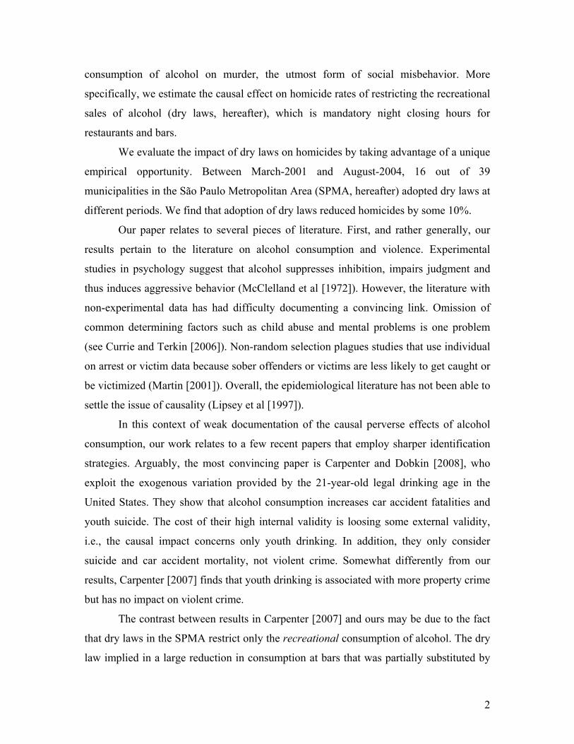
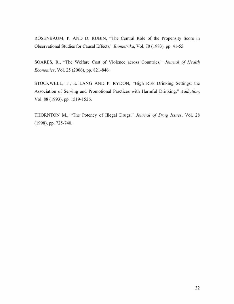
The story of the paper can be summarized by figure I. Panel A shows several

facts. Not surprisingly, adopting cities were more violent than non-adopting ones before

adoption. Nevertheless, homicides were falling at about the same rate in both groups of

cities. Following adoption, homicides dropped much faster in adopting cities. The

difference in slopes means that, after adoption, homicides dropped 14 percentage points

more in adopting than in non-adopting cities. For adopting cities, the difference in slopes

before and after adoption is statistically significant; for non-adopting cities it is not

statistically significant. In panel B, we regress the homicide rate on city and time

dummies, and a set of dummies for months before and after the adoption. Estimated

coefficients are depicted. Two things are noticeable: a sharp drop in homicides at the

month of adoption, and a change in levels before and after adoption.

Is figure I indisputable evidence that dry laws had a causal impact on homicides?

The answer is no for several reasons. First and foremost, adoption is a choice of cities,

which poses several challenges for causal inference. One such challenge is that dry laws

could have been adopted exactly where they would work, although we find this

possibility quite unlikely. It relies on an implausible level of rationality and

foresightedness on the municipal-level policy makers.

5

More importantly, endogenous adoption suggests that adopting cities may have

adopted other crime-fighting policies. This is all more likely because adopting cities were

particularly violent prior to adoption (figure I, panel A). Although we control for a long

list of “other suspects”, it is always possible that dry law is confounded with the adoption

of other unobserved policies. Additionally, adopting and non-adopting cities may be

different in time-varying dimensions. For example, homicides could be following

different secular trends prior to adoption (although figure I suggest this is not the case).

Finally, and again because adopting cities were more violent prior to adoption, mean

reversion could mechanically produce the results.

The paper is organized as follows. Information on data sources is in Section 2.

Section 3 describes the empirical setting and narrates the chronology of the events.

Section 4 contains an extensive description of the empirical strategy designed to address

the difficulties raised by the non-random adoption of dry laws. Results are presented in

section 5, which also contains an extensive robustness analysis, validation and

falsification tests. Section 6 discusses other policy interventions and alternative

explanations for our results. Section 7 concludes.

2. Data

Data come from several sources. Crime data are from the “Secretaria Estadual de

Segurança Pública de São Paulo”, the state-level enforcement authority. Data runs from

April 1999 through December 2004. The sample ends in December 2004 because it is the

last month for which monthly data was available. For validation purposes, we use data on

deaths by car accidents from DATASUS, a hospital database from the Ministry of Health.

We use both city-level data, and report-level data from INFOCRIM, a compustat crime-

tracking system. Report-level is useful because it contains information on the time of the

day the crime was committed.

INFOCRIM started in 1999 in the city of São Paulo. In other cities in the SPMA,

it was implemented gradually, as precincts were incorporated in the system. Thus, cities

enter the sample as INFOCRIM was implemented at its precincts. Since INFOCRIM was

not operational in all cities during the sample period, we use it only as corroborative

6

evidence. Still, INFOCRIM does have data on adopting and non-adopting cities (mainly

São Paulo) before and after adoption, and thus it is rather useful for our purposes.

Although crime data usually suffer from under-reporting, our three main

dependent variables - homicides, deaths by car accident and vehicle robbery – are well

measured. In the case of murder under-reporting is negligible because an investigation is

mandatory as long as body is produced.1 Reporting is also mandatory in case of deaths by

car accident. Finally, vehicle robbery is well measured for three reasons: avoiding

receiving traffic tickets; avoiding having one’s name involved in criminal activities

related to the subsequent use of a stolen car; and for insurance purposes.

A small digression on under-reporting is in place because we use other crime

categories such as battery as corroborative evidence. Crime statistics suffer from serious

under-reporting in Brazil, stemming from historical general lack of confidence on police

authorities. Under-reporting per se does not mean that information from other categories

is useless, only that extra caution must be exercised because under-reporting dropped

over the period. State-level police action has improved, and thus improving reporting.

Institutional improvement in the state-level bureaucracy reduced the costs of reporting.

Among them are i) Poupa-Tempo, whose claque is “time-saver”, and corresponds to the

creation of offices where all state requirements to the citizens such as getting documents,

using the judicial system, paying bills and reporting crimes are pooled together; ii)

Delegacia Eletrônica (electronic police station) for on-line reporting and iii) Delegacias

da Mulher, police stations specialized in domestic violence.

Recorded crime rates confirm that under-reporting dropped over period. Figure V

shows three categories: homicides, vehicle theft/robbery and common theft/robbery,

which includes all categories except vehicle. In 1999 vehicle and common theft/robbery

rates were similar, an evidence of under-reporting. In the United States, recorded

common theft/robbery is three times higher than vehicle theft/robbery (Uniform Crime

Report, 2006, FBI). Overtime, homicides and vehicle theft/robbery follow a similar

pattern of reduction, reflecting the general drop in crime in the SPMA due to factors

1 Homicides are attributed to a city if the crime was committed in that city or if the dead body was found within the city limits. Some “miscoding” happens because the dead body could be moved. Except for very elaborate stories, this only introduces noise in the homicide data.

7

discussed in section 3. In contrast, common theft/robbery, if anything increased during

the period, which is hard to rationalize except for improvements in reporting.

If these improvements occurred uniformly across cities, there would be little

concern in using under-reported categories. However, reporting did not improve

simultaneously across cities. Poupa-Tempo started in São Paulo City. Delegacia

Eletrônica was available across the state, but internet penetration varied wildly both

across cities and over time. For all these reasons, under-reported categories are used only

as additional evidence and with caution.

Demographics are from Fundação SEADE, a state-level government think-tank

that compiles data for São Paulo State from several sources. Besides conducting their

own surveys, SEADE compiles census data from Instituto Brasileiro de Geografia e

Estatística (IBGE), the Brazilian equivalent of the Bureau of Statistics. From their

database we have annual city-level income per capita, population and male population

between 15 and 30 years olds. Since our procedures use monthly crime and accident data,

we interpolate these demographics to obtain a monthly frequency. Also from Fundação

SEADE comes information on other policies such as the presence and the date of

establishment of a municipal police force (if any), its size, spending on education and

welfare, and the creation date of a municipal secretary of justice (if any). Information on

the dry laws comes from the text of the law, which we collected on-line or requested to

the city council by telephone.

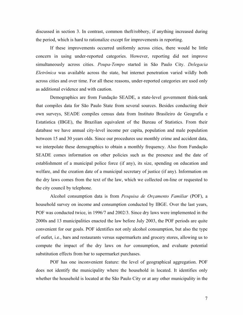
Alcohol consumption data is from Pesquisa de Orçamento Familiar (POF), a

household survey on income and consumption conducted by IBGE. Over the last years,

POF was conducted twice, in 1996/7 and 2002/3. Since dry laws were implemented in the

2000s and 13 municipalities enacted the law before July 2003, the POF periods are quite

convenient for our goals. POF identifies not only alcohol consumption, but also the type

of outlet, i.e., bars and restaurants versus supermarkets and grocery stores, allowing us to

compute the impact of the dry laws on bar consumption, and evaluate potential

substitution effects from bar to supermarket purchases.

POF has one inconvenient feature: the level of geographical aggregation. POF

does not identify the municipality where the household in located. It identifies only

whether the household is located at the São Paulo City or at any other municipality in the

8

SPMA. Thus, comparing precise groups of adopting and non-adopting municipalities is

not feasible using the POF. Nevertheless, we can compare a group of cities that contains

adopting cities and a group that does not contain any adopting city. Quite important for

our purposes, 69% of the population in the SPMA excluding the city of São Paulo lived

in adopting cities. Finally, field work was done between July 2002 and July 2003.

Luckily, 71% of the adopting cities’ population was in cities that have adopted in or

before July 2002. Another 18% of adopting cities’ population was in cities that adopted

between August 2002 and July 2003. Hence, most dry laws were effective when

interviews were conducted.

3. The Empirical Setting and the Chronology of Events

The SPMA is the largest contiguous urban area in South America, and the third

largest worldwide. Politically, it is defined as an administrative region in the state of São

Paulo. In 2005 it had roughly 19 million inhabitants. It is composed of 39 independent

municipalities, with their own mayor and city council. City sizes vary widely, from Santa

Isabel with a population of 11,000, to São Paulo City, with its 11 million inhabitants in

2005.

Although violence has gone down over the last 8 years, the SPMA is a violent

place. Figure II, which is a broader version of figure I, shows the evolution of homicides

over the 1992-2004 period. Homicides increased steadily through the 1990s reaching a

peak in 1999. They subsequently fell sharply, a reversion comparable to that of New

York in the 1990s. Several factors contributed to this reversion. For example, De Mello

and Schneider [2008] show that changes in the demographic pyramid trace very well the

time-series pattern of the data: the SPMA experienced an increase in youngsters (between

15 and 24 years old) in the 1990s and a reduction in the 2000s.

In reaction to the sharp increase in crime during the 1990s, but after the reversion

in 1999, policy interventions took place in every level of government. Perhaps the most

famous are (i) the Lei do Desarmamento (Dec-2003), a federal legislation on firearms’

possession, and (ii) INFOCRIM, a compustat-like crime-tracking system that improved

police intelligence at the state level. We have no credible quantitative measure of their

9

impact, but it is likely that they contributed to decline in homicide depicted in figure II.

For our purposes, however, it is important that that these two policy interventions cannot

be confounded with the dry laws (see discussion in section 6).

Municipalities have jurisdiction over the regulation of local commerce. This

allowed Barueri, a city in the SPMA, to approve in March 2001 a legislation imposing

mandatory closing hours for bars and restaurants, from 11PM to 6AM. The law allowed

for exceptions, under certain circumstances. In Barueri, less than 60 bars and restaurants

out of roughly 4,000 were exempt.2 Several cities followed suit, and as of December

2004, 16 out of 39 cities in the SPMA have adopted similar legislation. While laws varied

somewhat in strictness, with a few adopting cities having laxer rules during weekends,

71.68% of the population in adopting cities were in municipalities where the curfew at

11pm was in place all week, and all municipalities but Osasco have a curfew at 11pm

during weekdays. Table I has the adoptions dates and the closing hours.

Anecdotal evidence suggests that the laws worked. One newspaper story is

particularly illustrative. The owner of a bar in Diadema, a particularly violent adopting

city, reports that “…before [adoption] it was a little messy here. The law is good because

it avoids fights.”3

Taken together, adopting cities had a population of 3.2 million inhabitants in

2004, and accounted for 17% of the population in the SPMA. Excluding the São Paulo

City, an outlier with 10 million inhabitants, dry laws were adopted in cities that account

for 46% of the SPMA.

In weak institutional settings such as Brazil, it is not obvious that dry laws were

actually enforced, i.e., whether bar consumption of alcohol dropped as a consequence of

adoption. Again, anecdotal evidence suggests that the laws were effective. In the same

newspaper story, the husband of the bar owner reports that “…sales have fallen after the

2 Conditions for exemption included not being located near schools, being outside “crime zones” or zones without nuisance complaints. The presence of acoustic isolation and of private security in front of bar was also a necessary condition. See http://www.propagandasembebida.org.br, in Portuguese 3 This story is at Globo Online, the electronic version of the second most important newspapers in Brazil. In Portuguese at http://g1.globo.com/Noticias/SaoPaulo/0,,AA1359613-5605,00.html. The Economist, 10/20/2005, reporting a story on Diadema (an adopting city in the SPMA), lists dry laws as an important factor contributing for the decline in murder rates starting in 2001. In an interview to O Globo, the second largest circulation newspaper in the country, Barueri's (another SPMA city) Municipal Secretary of Communication reports that homicides "fell up to 70%" after the city implemented the dry law.

10

law was passed”. We confirm this anecdotal evidence using household consumption data

from Pesquisa de Orçamento Familiar (POF). POF allows us to compare alcohol

consumption patterns between 1996 and 2003 in the city of São Paulo and the rest of

SPMA.

We calculate the impact of dry law adoption on the consumption of two alcoholic

beverages: beer and cachaça, which represent roughly 82% of total alcohol consumption

in value (figures are from POF).4 We estimate the following model:

itittitiit CONTROLSSPMASPMAAlcohol εγγγγ +Σ+×+++= 20032003 3210 (1)

where SPMA is a dummy for the SPMA excluding the city of São Paulo; and 2003 is a

dummy that equals 1 if the interview was done in the 2002-2003 POF. Controls include

gender, age, years of schooling and household income of the respondent. Alcohol is

measured both as a fraction of total consumption in bars, and as total consumption. POF

has a stratified sampling design so we use weights to make observations representative of

the population.

Table II shows the percentage of alcohol consumption in bars/restaurants versus

supermarkets/grocery stores. The pattern is clear. In 1996, for both beer and cachaça, bar

consumption as a fraction of overall consumption was similar in the two groups of cities.

The picture changes in 2003. The percentage of bar consumption of cachaça remained

roughly constant in the city of São Paulo. In contrast, it dropped nine percentage points in

the SPMA excluding São Paulo. Bar consumption of beer dropped in both groups but

much more pronouncedly in the SPMA excluding the city of São Paulo. Averages

suggest that the adoption of the dry law caused a 23.61 and an 11.11 percentage point

reductions in bar consumption of beer and cachaça, respectively. Columns (1) and (3) of

table III shows that this difference is statistically significant. In column (2) and (4) we see

that these differences are larger after controlling for demographics. Interestingly, males

are more prone to consuming alcohol in bars, as expected, providing further evidence that

dry laws had the potential for reducing violent crime. 4 Cachaça is the national alcohol beverage, distilled from fermented sugar cane. Its alcohol strength ranges from 38%/Vol. to 48%/Vol.

11

The remaining columns in table III concern total consumption. For both beer and

cachaça, bar consumption in the dry law group dropped in absolute terms and relative to

the control group (columns (5) and (7)). The reduction in consumption is economically

significant. Take cachaça for example. The 121.473 drop in annual consumption of

cachaça attributable to the dry laws represented roughly one half of a monthly minimum

wage in 2000. Columns (6) and (8) show the same estimates for supermarket/grocery

store consumption. In both cases some substitution occurred: supermarket consumption

increased in the SMPA excluding the city of São Paulo. For cachaça the substitution

effect is small, representing no more than 14% of the reduction in bar consumption. For

beer, the substitution effect is large, some 111% more than the reduction in bar

consumption. These estimates confirm the intuition in the industry that cachaça is a “bar

drink”, especially in the poor neighborhoods of edge cities.

In summary, individual consumption data shows that dry laws worked towards

reducing bar consumption, both overall and relative to total alcohol consumption. Some

substitution occurred but not enough to offset the overall reduction in alcohol

consumption, especially in the case of cachaça.

4. The Empirical Strategy

Our identification strategy hinges on six pillars. First, we use both time-series and

cross-section variation. Thus we can control for all time-invariant heterogeneity across

cities, a necessary condition to make causal inference on any alcohol-crime relationship.

Several common determinants of crime and alcohol (ab)use – such as child abuse,

poverty, and psychological disturbances – are almost never observable, and are fairly

constant over short periods of time. Second, the staggered nature of adoption provides an

additional source of identifying variation. Different adoption periods allow us to compare

early adopting cities with late adopting cities, thus mitigating the problems posed by

endogenous adoption. Third, dry laws should have different impacts on different types of

crimes, a feature that allows us to isolate the impact of potential adoption of other non-

observable policies; in other words, other crime categories provide the basis for

validation and falsification tests. Fourth, if dry laws did have a causal impact on

12

homicides, then the distribution of homicides during the day must have changed in

response to the restriction in bar opening hours. Fifth, we analyze the institutional and

empirical determinants of the adoption of dry laws and other crime policies, and show

that i) adoption of dry laws does not seem to correlate with the adoption of other

observable municipal level policies; and ii) the institutions of law enforcement in the

state of São Paulo make it highly unlikely that law enforcement could not have spuriously

produced the results. Finally, we conduct an extensive sensitivity analysis to probe the

robustness of our results.

4.1 Summary statistics: Adopting and Non-Adopting Cities

Summary statistics on adopting and non-adopting cities are presented in table IV.

The SPMA is a violent metropolis. In our six-year sample, 45,400 people were murdered

in the SPMA. With a population around 18 million people over the period, the average

monthly rate of homicides was 3.65 per 100thd inhabitants. For comparison, in 2002, the

SPMA would rank second in the United States, slightly below Washington DC, the

“murder capital”, with its 3.81 monthly homicides per 100thd inhabitants. In Chicago, the

5th most violent city, the rate was 1.85. In New York City at its peak (1990), the rate was

3.56.

Non-adopting cities resemble adopting in most dimensions, a desirable feature of

a “control group”. They are similar in terms of population, percentage of male population

between 15 and 30 years old, income per capita, and school attainment measured both by

the number of years of schooling and by the high-school drop-out rate. The first row in

Demographics seemingly suggests that non-adopting cities are larger than adoption. This

difference is driven by city of São Paulo, which represents 58% of the population of the

SPMA. Excluding São Paulo, adopting and non-adopting cities have roughly the same

average size.

Average characteristics may disguise time-series heterogeneity. Data, however,

suggest that demographics in adopting and non-adopting cities followed similar secular

trends. Comparing the first and the last 6 months in sample period, nominal per capita

income rose by 31% and 27% in adopting and non-adopting cities, respectively. The

13

proportion of population in the crime-prime age (male in the 15-30 age bracket) dropped

by the same magnitude in both groups. Population growth is also similar.

As we know, dry laws were adopted in more violent cities. Over the sample

period, monthly aggregate homicides in adopting cites averaged a rate of 3.83 per 100thd

inhabitants, roughly 7% higher than the 3.59, the rate of non-adopting cities.

Comparing averages before and after adoption suggests that the adoption of dry

laws is associated with a drop in homicides. In adopting cities, the monthly homicide rate

was 2.32 in the last 6 months of the sample period, a 97% drop from 4.57 in the first 6

months of the sample period. Homicides also fell in non-adopting cities over the same

period by 87%. This “difference-in-differences” represents a 10% drop in homicides to

be attributed to dry law adoption, in line with the 14% suggested by figure I.

Before proceeding to confirm the suggestion of the difference in means, we do an

in depth investigation of the determinants of the decision to adopt the dry law.

4.2 Investigating the decision to adopt the law

In the context of non-random determination of dry law adoption, two points are

crucial for causal inference. First, if adoption occurred in reaction to surges in homicides,

then it is likely that other unobserved policies were adopted concurrently. Second, if

observed policies explain dry law adoption, then it is likely that all policies – observed

and unobserved - were also adopted in bundle. We estimate a duration model for the

timing of adoption to evaluate the empirical relevance of these two points (see Kiefer

[1988] and Jenkins [1995]). The following factors are included in the duration analysis:

• All municipal policy variables whose data is available. Policies are divided in two

sets: a) law enforcement policies, such as presence of a municipal secretary of

justice, of a municipal police force, their adoption time if they were established

during the sample period, and the size (in personnel) of the municipal police force

(in 1999 and in 2003); and b) policy choices that are arguably related to crime

prevention, such as the municipal expenditures on welfare (social assistance),

education, and cultural activities.

14

• The recent dynamics of homicide. This allows us to test the hypothesis that dry

law adoption was related to recent shocks to homicides. We also include the

average homicides in 2000 as a baseline measure of homicides to measure how

overall violence affects the decision to adopt.

• Demographic controls such as income, population and male population between

15 and 30 are included because they may affect homicides and, potentially, the

decision to adopt dry laws (a younger constituency may oppose the adoption). In

two of the specifications time and time squared are included to account for time

varying hazard rates. Adoption occurs over time and, as figure I makes clear,

homicides follow a decreasing trend overall in the sample period. Hence, time

affects both adoption and homicides.

• Finally, the number of neighboring cities that have adopted the law at time t is

included. It captures neighbor emulation or adoption for fear of suffering from

spillover effects. Table IV presents the results.

The first column contains the results of a stripped-down model. Neither the

dynamics of homicide nor competing policies are included.5 In line with descriptive

statistics, demographics are unrelated to the adoption of dry laws. Time explains adoption

mechanically because adoption occurs later in the sample period. Base line homicides in

2000 increase the hazard rate of adoption, meaning that more violent cities were more

prone to adopt. Finally, the number of adopting neighbors also increases the hazard rate,

suggesting either an imitation effect, or adoption for fear of spillover effects. Taken

together, these variables explain 15% of the timing of adoption of dry laws.

The model presented in column (2) includes four lags of homicide. None is

significant individually, all lags are jointly insignificant. In column (3), homicides are

omitted and all observed competing policies are introduced. Neither the establishment of

a municipal police force nor of a secretary of justice affects the hazard rate. Similarly, the

hiring of new municipal policemen does not affect the timing of adoption. Finally, 5 The sample is restricted to the period September-1999 through December-2004 to maintain the sample uniformity across estimated models (when the four lags of homicide are included, observations from April-1999 through August-1999 are lost). Results in columns (1) and (3) (where it matters) are very similar if the May-August observations are reintroduced.

15

spending in education increase the hazard rate of adopting dry laws, but welfare spending

reduces it. Overall, all competing policies explain an additional 6 percentage points

(above and beyond the variables included in column (1)) of the timing of adoption of dry

laws.

Column (4) is a combination of columns (2) and (3), with all the variables

included. In column (5), we include only the main variables of interest: the dynamics of

homicide and the competing policies. Results are similar: past homicides are still

unrelated with the timing of adoption, and only spending with education and welfare are

related to the adoption of dry laws. It is noteworthy that lags of homicides and competing

policies explain half the variation explained by demographics, the number of adopting

neighbors, and baseline homicides (8% against 15%).

In summary, the main drivers of adoption are the number of adopting neighbors

and how violent the city was in 2000. Among other policies, only spending in

“preventing measures” is related to dry laws, but only weakly and in an inconsistent way.

Welfare has the wrong sign, for example. We interpret these results as follows: violent

cities decided to adopt as a measure to fight crime, and neighbors followed suit, perhaps

because of anecdotal evidence that dry laws worked, or maybe because they feared

spillover effects. Insofar as it suggests that observed crime-fighting measures were not

adopted in bundle, this evidence increases our confidence in interpreting our results as

causal.

4.3 The Empirical Model

We estimate several version of the following model:

itit

I

iii

T

tttitit

CONTROLSCity

MonthAdoptLawHomicide

εη

ωββ

+Φ++

++=

∑

∑

=

=

1

110

(2)

where i is a city in the SPMA, and t is a month. AdoptLawit is a dummy variable that

assumes the value 1 if the dry law was in place in city i at period t, and 0 otherwise.

Hence, for non-adopting cities, it assumes only the value 0. We test whether the

16

parameter β1 is negative, i.e., whether dry laws reduced homicides. Montht is a full set of

period dummies. Their inclusion is important because homicides were falling in the

SPMA as a whole. If period specific effects are not accounted for, AdoptLawit will

capture aggregate shocks because it assumes more values 1 at the end of the sample

period. Cityi is a full set of city specific dummies to control for city fixed-effects.

Although model (2) discards all pure cross-sectional and all pure time-series

variation, objections to causal interpretation still arise. First, the procedure does not

account for all time-varying heterogeneity. This is always true in any policy evaluation

procedure, but it is a more serious threat when policy adoption is a choice.

The most direct way to account for time-varying heterogeneity is including

controls. Controlsit includes income, population, and the percentage of population in a

particularly problematic age bracket, between 15 and 30 years. These demographic

variables affect homicide and are observed with at least an annual frequency. We are

agnostic as to whether these variables affect adoption of dry laws but, since they are

available, there is little objection to inclusion. More importantly, all observable

municipal-level policy changes that occurred during the period are included (which are

the same as in the duration model of adoption).

Although section 4.1 and figure I.A suggest that different results will not be

driven by different secular trends in homicides, we play it safe and we implement three

procedures to account for them. The first consists in estimating a “random-trends” model;

each city has its own specific linear trend θit. Alternatively, we estimate a rich dynamic

model. In some specifications, Controlsit includes several lags of the homicide as

explanatory variables. An additional advantage of including lags of homicides is the

following. Despite evidence in section 4.2, it could still be the case that spikes in

homicide induces both the adoption of dry law and of other unobserved policies. By

including lags of homicide we proxy for these unobserved policy reactions. There is no

specific theoretical reason to believe that past homicides cause present homicides, after

time and city specific effects are included. However, a rich dynamic model serves a dual

purpose: controlling for different secular trends and proxying for possible unobserved

policy reactions.

17

Finally, we perform a placebo experiment, in which AdoptLawit assumes the value

1 a year before it should. If estimates are similar, one would have serious reasons to

suspect that something else drives the results. In particular, one would suspect that

different secular trends, not adoption of dry laws, are the main culprits.

We weight observations by population. The data is at the city level, and city size

varies wildly within the SPMA. Weighting by population serves a dual purpose. First, it

emulates a regression at the individual level i.e., weighting observations provides

estimates closer to a random sample in the SPMA. Second, homicides are not a common

occurrence, and observations from small cities are much noisier than those from larger

cities, i.e., the variance of εit is decreasing in population (see standard errors of homicide

rates by city size in table V). Thus variation from smaller cities should be discounted. In

order to avoid giving more weight to observations in the later part of the sample, the

weight is the city population in 2000. Finally, observations are always clustered at the

city level. Thus, all estimated standard errors are robust to within city correlation, an

important feature in light of results in Bertrand et al [2004].

5. RESULTS

5.1 Main Estimates

Table VI shows estimates of several versions of model (2). For conciseness, only

1β̂ is reported. Other estimates are available upon request. All models include a full set

of city and period dummies.

Column (1) contains the estimates of the simplest model, with no time-varying

controls (besides period dummies). The estimated coefficient on the variable AdoptLaw

( 1β̂ ) is -0.642, and it is reasonably well estimated (p-value = 5.73%). Considering the

homicide rate in adopting cities in the six first months of the sample (4.57 in table

V), 642.0ˆ1 −=β means a 14% drop in homicides per 100thd inhabitants, a significant

reduction. In terms of lives, had the law been adopted in the city of São Paulo (more than

18

10 million inhabitants), this would mean roughly 770 (0.642×100×12) lives saved

annually.

Results in columns (2)-(4) show that the estimated impact of dry law adoption is

robust to inclusion of controls. In fact, including competing policies increases the

estimated effect of dry laws (t is now 0.847), and increases precision (p – value = 3.54%).

In column (3) four lags of homicide are included as regressors. The estimated coefficient

is now smaller in magnitude (0.510) but still quite significant both practically and

statistically (p – value < 1%). In column (4) we include the observed time-varying

demographics and the number of adopting neighbors. Since it is the most complete

model, the point estimate -0.490 is our benchmark estimate for the impact of the dry law.

Table VII presents a long list of robustness checks. First, we check whether the

weighting procedure is driving results and estimated the model by straight OLS, without

weighting (column (1)). Comparing with the benchmark (column (4) on table V), point

estimates are similar but the estimated standard errors are larger under OLS, which

confirms the efficiency of the weighting scheme. In Column (2) we use WLS again, but

exclude the city of São Paulo because it represents 60% of the sample in terms of

population. The point estimate (-0.679) is larger than the benchmark -0.490.

Column (3) deals with the econometric challenges posed by the inclusion of lags

of the dependent variable. The fixed-effect transformation does not work if N is large and

T small, unless the error term is strictly exogenous, which rules out serial correlation for

example. Since in our case N is small and T is large, OLS has small bias but Monte Carlo

experiments suggest one needs large N and very large T. Despite the complications in

identifying models with fixed-effects and lagged dependent variables, we implement a

GMM procedure, using further lags as instruments for the lags of the included lags of

homicide (Arellano and Bond [1991]).6 The point estimate is larger (in modulus) than the

benchmark (-0.536 versus -0.490). Thus, potential biases caused by inclusion of lags of

the dependent variable are towards zero, if anything.

6 A wide range of possible specifications for the Arellano-Bond estimator is available. For conciseness reasons, and because this is only one of the many robustness check, we do not dwell into the several implications of different estimation methods. We implement the standard version on the STATA package. All variables are first-differenced, the one-step estimator for the standard deviation is used and Ti – p – 2 lags are used as instruments for the p included lagged dependent variable. Only one slight modification: four lags (the p) of the dependent variable are included (instead of two).

19

In Column (4) the model is estimated in logs, with very similar results. The

estimated coefficient means that dry laws cause a 15.2% reduction in homicides.

Homicides were higher in adopting than in non-adopting cities around the period

of adoption. This suggests that mean reversion may be driving results. To deal with this

issue, we allow each city to have its own linear trend θit. Columns (5) (no dynamics) and

(6) (full model) show results very similar to previous estimates.

Finally, in column (7) we perform a placebo experiment in which AdoptLaw is

replaced by a faux treatment dummy that assumes the value 1 twelve months before

actual adoption. Although negative, the estimated coefficient associated with the faux

treatment is almost five times smaller in modulus than the benchmark -0.490 (and it is not

statistically significant).

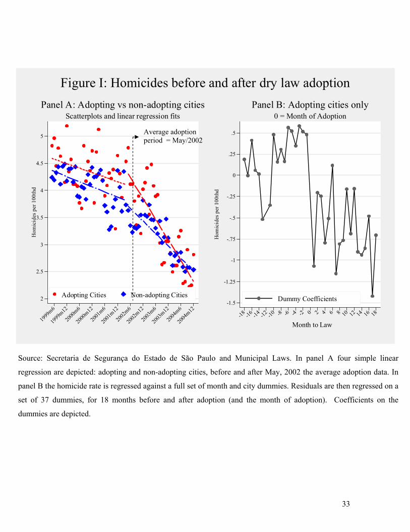
Figure III presents the coefficients of a different specification. The spirit is similar

to Panel B in Figure I but controls are added to the specification. Treatment is coded as a

set of dummies for the number of months to the introduction of the law. A total of 36

dummy coefficients are estimated, 18 for the months before and 18 for after the law. Two

patterns arise. Before adoption, the estimated dummies are all zero, except for the 12th

month before adoption, a positive outlier. At the month of adoption, we estimate a big

negative coefficient on the dummy. For subsequent months, the dummies fluctuate

around -1, which is in line with the hypothesis that dry law had a causal impact on

homicide.

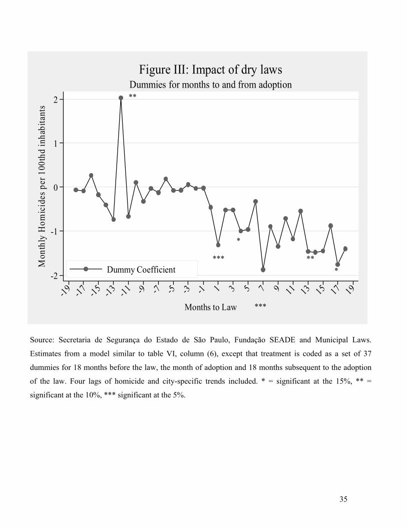
A final piece of evidence comes from INFOCRIM, which has report-level data,

with which we trace the hour of the day that homicides were committed. INFOCRIM is

collected since 1999 for the city of São Paulo. Luckily, compilation includes some (but

not all) observations from neighboring cities. Among them are Diadema and Osasco, two

adopting cities. Thus we can compare the distribution of crime throughout the day in

adopting and non-adopting cities before and after adoption. Figure IV has the results.

The histogram in the right shows the distribution of homicides throughout the day

in the city of São Paulo. Two histograms are overlaid, one for the years 1999-2001,

another for 2002-2003. No noticeable change arises, as expected. In adopting cities the

figure is different, and a clear pattern arises. After adoption, the proportion of homicides

that occurred between 11pm and 6pm (closing hours in Diadema) dropped significantly,

20

from 44% to 32%. In line with the hypothesis that the recreational consumption of

alcohol induces violence, the distribution of homicides in adopting cities shifted to the

7pm-22pm period, which are the night opening hours for bars. These results are strong

because it is difficult to conceive a policy change or demographic shift that caused a shift

in the distribution of homicides throughout the day.

5.2 Using only adopting cities

Adoption did not occur simultaneously across cities. Thus, we can restrict the

analysis to adopting cities and use only the staggered nature of adoption as the source of

identifying variation. In this case, adopting cities before adoption become the control

group.

Restricting the attention to adopting cities involves a variance-bias trade-off.

Clearly, excluding non-adopting cities discards relevant variation and increases variance.

On the other hand, restricting the sample to adopters reduces potential bias for two

reasons. Late adopters have a very high “propensity” to adopt, given that they eventually

did adopt, thus helping “homogenize” the control and treatment groups.7 Second, it

reduces the risk of capturing potential unobserved policies. It could still happen that late

adopters could also have adopted unobserved policies later, and the effects would still be

confounded. However, the “unobserved policies bias” now needs a very fine tuning of

timing to work. Table VIII contains the results.

Column (1) is the equivalent of the benchmark model (Table VI, column (4)).

Results are, if anything, stronger. Although as expected some precision is lost, the

estimated coefficient is still rejected at the 5% level. In column (2) we restrict the sample

to December 2003 to emulate the case of a treatment and control groups with late

adopters as controls. Results are again stronger. In column (3) we include city-specific

dummies but exclude the dynamics of homicide. Results are similar. When both are

7 Previous versions of this paper contained the results of a propensity score weighting procedure. More weight was given to adopting city-month pairs that had a lower probability of having a law in place, and vice-versa for non-adopting cities, in the spirit of Rosenbaum and Rubin [1983] and Imbens [2000]). The observables of the propensity function (probit) were the same variables included in the duration model. Results, if anything, are slightly stronger, and are available upon request.

21

included we replicate the benchmark estimate (table VI, column (4)). Although precision

is lost we still reject the null hypothesis of no effect at the 10% level.

5.3 Validation Tests

Arguably, dry laws should have an impact on other outcome variables. As a

validation exercise we measure the impact of dry law adoption on deaths by car

accidents, and battery.

5.3.1 Impact of Dry Laws on Battery

As suggested by the newspaper story, dry laws reduced fights. Thus it should

have an impact of crime against a person that come short of murder. The Brazilian Penal

Code has a category called Lesão Corporal Dolosa, whose literal translation is Body

Injury with Intent. Its equivalent in Common Law is battery.8 Table IX shows descriptive

statistics on battery and table X contains the results of the estimates of some models in

tables VI-VIII. For the sake of brevity we do not show estimates from all models (which

are available upon request).

Column (1) – (3) show that, regardless of the inclusion of controls, dry laws

reduced battery. Consider the estimate -2.915 in column (3), the equivalent of the

benchmark model for homicides in table VI, column (4). Comparing with means in table

IX, this coefficient represents roughly 10% of battery in adopting cities, an impact very

similar to that on homicides. Again, using only the staggered nature of adoption to

estimate the impact (column (4)) does not change results significantly.

5.3.2 Impact of Dry Laws on Deaths by Car Accident

Unfortunately, we have no data on accidents or alcohol related hospital

admissions but hospital data on deaths by car accident is available. Table XI presents 8 Assault is normally defined as the threat of violence, while battery is actual physical violence. We do not have data on “attempted” Lesão Corporal Dolosa, which should be roughly similar to assault.

22

summary statistics on deaths by car accident and Table XII shows results when the

dependent variable is deaths by car accidents.

Results suggest that dry laws had an impact on deaths by car accident. Point

estimates suggest that adoption of dry laws reduced car accidents casualties by roughly

0.055 deaths per 100,000 inhabitants. In terms of magnitude this effect is a little smaller

than the impact on homicides. It represents 8.5% reduction in car accident deaths. It is

however much less precisely estimated, which is not surprising for several reasons. First,

the relationship between bar drinking and deaths by car accident is much more tenuous

than the relationship between homicides and bar drinking. For once, the vast majority of

bar drinkers, ca accidents are not relevant because about half of the population in the

SPMA during the period of analysis did not have a car. Most bars are in the periphery,

whose dwellers use the public transportation system; drunk driving (whose law started

being enforced now) is more a problem in middle-class and upper-middle class places,

which represent a small proportion of population and bars. Second, the geography of the

relationship between bar drinking and deaths by car accident is unfavorable. It is unclear

whether an accident will happen at the city where the bar is located, or another city. For

homicides, odds that the homicide will be committed nearby are higher simply because

committing homicides do not imply driving (deaths by car accident necessarily imply

someone driving). On top of that, hospital data is problematic. The Emergency Room

where the victim end up may not be in the same city where the bar is located or the

accident took place. Finally, when the victim is declared dead at the scene she/he will be

taken to the morgue and consequently will not show in the hospital data. For these

reasons, hospital data on car accidents are very noisy.

To mitigate the influence of accidents that happen outside the adopting cities

limits, we discard the smallest half of adopting cities in terms of area. Results are now

comparable to those for homicides. In column (3), we also discard the smallest half of

non-adopting cities. Results are similar but precision is lost due to the small number of

observations.

23

5.4 Falsification Tests

In this subsection we use crimes that should not have been affected for

falsification tests. If we find an impact of dry law on such crimes it would raise suspicion

that estimated impact of the dry law is spurious and should be attributed to “other

unobserved crime-fighting policies”.

5.4.1 Impact of Dry Laws on Vehicle Robbery

Our preferred falsification crime is vehicle robbery because of accurate reporting.

However, accurate reporting does not make vehicles robbery a good falsification

category. If it was an impulsive crime it would be affected by dry laws. It is hard to argue

that the dampening inhibition effect of alcohol does not induce all sorts of bad behaviors.

Differently from homicides, however, there is less reason to believe that alcohol

consumed socially would have a pronouncedly larger impact on vehicle theft/robbery.

However, the main argument is the nature of vehicle robbery in the SPMA. It is

well-known, but hard to quantify, that that vehicle theft/robbery is a professional crime,

driven by secondary market for parts and, to a less extent, by smuggling to neighboring

states and countries. This is hardly an impulsive type of crime. Mr. Schneider, one of the

authors and a former deputy secretary of security for the state of São Paulo reports that

the professional nature of this category is a known fact among enforcement authorities.

Second, there is an “impairment effect”: alcohol consumption compromises physical

motion and thus makes it hard to break into cars, especially because the use of security

devices. The odds of vehicle theft/robbery are substantial, with a rate of roughly 62 per

100thd inhabitants in 2004 (in US Metropolitan Areas the figure is 40 -Uniform Crime

Report, 2004, FBI). Not surprisingly, most car owners have U-locks, alarms, gas-

shutting-down systems, and even GPS tracking systems. This is true even when the

vehicle is insured because the premium increases substantially in the absence of

protecting devices.

All the arguments above apply for vehicle theft as well. However, robbery is a

better category for falsification because of the nature of the crime. By definition, since

24

robbery involves a threat, it occurs mainly in busy evening hours. Figure VI shows the

distribution of vehicle robberies during the day in the SPMA: only 20% of them occur

during the hours in which the dry laws are “binding”. For a comparison, consider panel

B, which shows the distribution of vehicle theft during the day. In contrast to vehicle

robbery, almost 36% of thefts occur during the dry law hours, 11pm-6am, which is the

mode of the distribution. This is unsurprising because theft does not require threat, and

the typical target is a vehicle parked in an empty street, i.e., late in the night and early in

the morning hours.

Table XII presents some summary statistics on vehicle robbery. First thing to

notice is that, differently from homicides and deaths by car accidents, noise in the

measure of car robbery is not related to the size of cities: both in magnitude and as a

percentage of the mean, standard deviations are not monotonically related to population.

Second, vehicle robbery is higher on average at adopting cities, due to the presence of the

city of São Paulo. Without São Paulo they are comparable.

Estimated coefficients are in table XIII. In columns (1) and (2), where more

parsimonious models are reported, the impact of dry law is positive but insignificant

statistically. When the full model is estimated, the impact is zero. Column (4) has the un-

weighted OLS estimate. Although the coefficient is much larger in modulus than in

column (3), it is still statistically insignificant. Even if it was precisely estimated, the

impact represents less than 1.2% of vehicle robberies in adopting cities (see table XII).

Thus, dry laws had no impact on car robbery, which reduces the possibility that we are

capturing “other unobserved policies”.

5.4.2 Impact of Dry Laws on Bank and Cargo Robbery

Besides vehicle robberies, we have monthly data from Jan-2001 onwards for bank

and cargo robbery, two good categories for falsification tests. Similarly to vehicle

robberies bank and cargo robbery should not be affected by dry laws, since both crimes

are professional. Bank robberies are complex ventures, which involve planning. Cargo

robbers need a network of contacts to dispose of the merchandise in the market. Similarly

to vehicle robbery, both bank and cargo robberies tend to be well measured because of

25

insurance reasons. Finally, both types of crime occur mainly during the daytime. Panel A

of Figure VII shows that 92% of bank robberies occur between 7am and 10pm, and 82%

percent between 7am and 6pm. This is expected because by definition robberies must

involve threat, and thus should almost always happen during bank opening hours.

Relative to vehicle robbery, bank robbery, and to lesser extent also cargo robbery,

has the disadvantage of being less frequent, which reduces the power of the test. Table

XV shows summary statistics for both categories. Table XVI presents the estimates of

same models presented in table XIV (vehicle robberies).

Start in panel A. The impact of dry laws on bank robberies is never different from

zero statistically, and the estimated coefficient is erratic, with oscillating sign. Bank

robberies are very infrequent, however, as the means in table XV show. Thus the failure

to estimate the impact of dry laws on bank robbery may be due to the low power of the

test. In panel B, we show the estimated impact of dry laws on cargo robbery, which is

much more frequent than bank robbery. Again, we never reject the null hypothesis that

the impact of dry laws on cargo robbery is zero. The estimated coefficient in column (1),

0.252, is large when compared to 1.008 (the mean of cargo robbery in adopting cities

(table XV)), seemingly suggesting that the impact is there but we have too little power to

identify it. However, notice that this large estimated coefficient is not robust to the

inclusion of controls: in all other three columns the impact of cargo robbery is

insignificant in practice as well as statistically.

5.5 Beggar-thy-Neighbor? Accounting for Spillover Effects

Adoption in a city may shift bar drinking to its non-adopting neighbors. Hence,

the control group could be affected by the treatment, introducing additional difficulties to

causal inference.

Table XVII shows several specifications that allow us to measure the spillover

effect, and assess its consequences. Columns (1) through (3) present direct evidence on

spillovers. The sample is restricted to non-adopting cities and adopting cities before

adoption, the “control group”. The main variable of interest is the intensity of neighbors

adoption, which is measured in three different ways: i) number of adopting neighbors, ii)

26

% of adopting neighbors and (iii) % of adopting neighbor population. In all three cases,

spillover effects are small and never significant, which we interpret as absence of

spillovers. In column (4) the sample is again full, and the number of neighbors with law

is interacted with the presence of dry law in the city: whether a dry law neighbor comes

across your boundary and drinks at your bars will depend on whether the receiving city

adopted the dry law. The estimated coefficient on the interaction, although positive, is not

significant, suggesting no spillover. Although the impact of dry law is seemingly larger in

adopting cities with few adopting neighbors, the difference is not statistically significant.

Despite their absence, we take the safe road and assess whether our results are

affected by spillovers. In columns (5) through (7) the sample is restricted to larger cities,

where there should be less concern that drinkers simply go to bars in non-adopting

neighboring cities. When population is the criteria for staying in the sample, results are

unaltered (columns (5) and (6)). However, physical size may be a better measure as it

captures more closely the costs of moving around. The estimated impact of the dry law is

now smaller, -0.294, but still statistically and practically significant. In summary,

spillover effects are neither relevant nor seem to impact our estimates in a significant

way.

6. DISCUSSION

In this section, we describe all other major policies that were adopted since the

late 1990s, and discuss whether it is plausible that they rationalize the results. Consider

police enforcement, which is not observable at the city level. Police arguably respond to

crime, and crime falls with increases in police (Marvell and Moody [1996], Corman and

Mocan [2000], Di Tella and Schargrodsky [2004], and Levitt [2002]). Although results so

far strongly suggest that adoption was not a reaction to spikes in homicide, it is still

conceivable that, for unknown reasons, police increased in adopting relative to non-

adopting cities precisely around the adoption periods. However, the institutions of police

enforcement in the state of São Paulo suggest otherwise.

Besides the fact that enforcement is done at the state-level, which considerably

reduces the potential endogeneity of police, the São Paulo state constitution mandates

27

that local police force size is determined every five years, based on the population.9 The

goal is keeping the same number of policemen per capita across cities. Some reallocation

could occur when several cities are covered by the same battalion. The police

organizational structure is as follows. The smallest unit is the police district, which is part

of a company that, in turn, is part of battalions, the largest unit. The number of policemen

is determined at the battalion level. There is some flexibility of allocating policemen

among battalions. The typical case, however, is one city-one battalion. Large cities may

have more than one battalion, and some battalions cover more than one city although it is

rare that the same battalion covers more than three cities. In summary, the institutional

setting significantly reduces the possibility of a major redeployment among cities in

response to crime within the time-span of our sample.

All major policies adopted in the period were at the state level, with a couple of

exceptions: the creation of the municipal security councils (state/municipal), and the

“disarmament law”. Municipal councils were created in 2006, outside our sample period.

By far the most publicized law enforcement event during the sample period, Lei do

Desarmamento - as it is known in Portuguese - was approved by the Congress on

December 22nd, 2003. It is a federal legislation and thus it affected all cities

simultaneously. Since law enforcement is done at the state level, we are not concerned

that its enforcement varied across cities. Moreover, since it was approved in late

December 2003, it could not plausibly affect results, especially when the sample is

restricted to December 2003.

The only major policy that could compete with dry law adoption is the creation of

INFOCRIM in 1999, a compustat-type geo-referenced system to follow real-time crime.

It is possible that INFOCRIM improved police efficiency and expediency in responding

to crime. However, it is quite unlikely that our results were confounded with INFOCRIM

since the ability to respond quantitatively to information based on the INFOCRIM was

only available in 2007 (see footnote 9).

In summary, it is implausible that these policies adopted over the last eight years

compete with dry laws in explaining the results. 9 Only recently, in 2007, has the rule changed. Now, an executive order allows the police commanders to use information from INFOCRIM when deciding on police force allocation.

28

7. CONCLUSION

At our benchmark estimate, dry laws reduce homicides rates by 0.490, which

means a 10.70% impact on adopting cities. On non-adopting cities, the counterfactual

effect is 11.72%.10 Since 16 out of 39 cities adopted, the Average Treatment Effect

(ATE) is 11.56%.11 Therefore, dry laws are responsible for a significant reduction in

homicides. To the best of our knowledge this is the first estimate of the impact of alcohol

restrictions on bars and restaurants on the rate of crime accounting for endogeneity and

that cannot be confounded with other policies or secular trends.

Our results provide a guarded support for policies that restrain the recreational

consumption of alcohol. We use the word “guarded” because in different institutional

settings results may not arise. Furthermore, our results are silent with respect to the cost

of implementing dry laws. Finally, we have to data to assess potentially perverse effects

of the law. In the UK, for example, police report data suggest an increase in violent

behavior right after 11pm, as pubs were closing (see Finey [2004]). A full cost-benefit

analysis should be conducted in order to assert confidently that opening hour restrictions

are worth implementing as a public policy.

Extrapolation to general alcohol consumption is not warranted. In fact, our results

are not in contradiction with the wisdom in economics literature. Prohibition and taxation

tend to fail because they do not reduce consumption, and may in fact shift consumption to

heavier “psycotropics”. Restricting recreational consumption is less radical and more

targeted than prohibition. The purpose is not preventing people from drinking, but

making it difficult for them to so in particularly dangerous settings.

REFERENCES

10 In the first six months of the sample, the weighted average homicides rates in adopting and non-adopting were 4.57 and 4.18. The effect is the coefficient 0.490 divided the weighted average and multiplied by 100. 11 This figure is the average of 10.70% (the treatment on the treated) and 11.72% (the counterfactual) weighted by average population in the first six months in the two groups (adopting and non-adopting).

29

BERTRAND, M., E. DUFLO AND S. MULLAINATHAN, “How Much Should We

Trust Difference-in-Differences Estimates,” The Quarterly Journal of Economics, Vol.

119 (2004), pp. 249-275.

CARPENTER, C. “Heavy Alcohol Use and Crime: Evidence from Underage Drunk-

Driving Laws,” The Journal of Law and Economics, Vol. 50 (2007).

CARPENTER, C. AND C. DOBKIN, “The Effect of Alcohol Consumption on Mortality:

Regression Discontinuity Evidence from the Minimum Drinking Age,” forthcoming

American Economic Journal of Applied Economics, Vol. 1 (2008).

CONLIN, DICKERT-CONLIN AND PEPPER, “The Effect of Alcohol Prohibition on

Illicit Drug Related Crimes: An Unintended Consequence of Regulation”, Journal of Law

and Economics, Vol. 48 (2005), pp. 215-234.

CORMAN, H. AND N. MOCAN, “A Time-Series Analysis of Crime, Deterrence and

Drug Abuse in New York City,” American Economic Review, Vol. 90 (2000), pp. 584-

604.

CURRIE, J. AND E. TERKIN, “Does Child Abuse Cause Crime?” NBER Working

Paper No. 12171, 2006.

DE MELLO, J.M AND A. SCHNEIDER “Age Structure Explaining a Large Shift in

Homicides: The Case of the State of São Paulo,” PUC-RIO: Texto para Discussão No.

549.

DI TELLA, R. AND E. SCHARDROSKY, “Do Police Reduce Crime? Estimates Using

the Allocation of Police Forces after a Terrorist Attack,” American Economic Review,

Vol. 94 (2004), pp. 115-133.

30

DUAILIBI, S, W. PONICKI, J. GRUBE, I. PINSKY, R. LARANJEIRA AND M. RAW,

“The Effect of Opening Hours on Alcohol Related Violence,” American Journal of

Public Health, Vol. 97 (2007), No. 12, pp. 2276-2280.

THE ECONOMIST, "Protecting Citizens from Themselves," 10/20/2005.

FINNEY, A., “Violence in the Night-Time Economy: Key Findings from the Research,”

Findings 214, Research Development and Statistics Directorate, Home Office, Her

Majesty Government, London, UK, 2004.

GORMAN D, P. SPEER, E. LABOUVIE AND A. SUBAIYA, “Risk of Assaultive

Violence and Alcohol Availability in New Jersey,” The American Journal of Public

Health, Vol. 88 (1998), pp 97-99.

IMBENS, G., “The Role of Propensity Score in Estimating Dose-Response Functions,”

Biometrika, Vol. 87 (2000), pp. 706-710.

JENKINS, S., “Easy Estimation Methods for Discrete-Time Duration Models,” Oxford

Bulletin of Economics and Statistics, Vol. 57 (1995), pp. 129-138.

KAHN, T. AND A. ZANETIC, “O Papel dos Municípios na Segurança Pública,” Estudos

Criminológicos, Vol. 4 (2005).

KIEFER, N., “Economic Duration Data and Hazard Function,” Journal of Economic

Literature, Vol. 26 (1988), pp. 646-679.

LEVITT, S., “Using Electoral Cycles in Police Hiring to Estimate the Effects of Police

on Crime: Reply,” American Economic Review, Vol. 92 (2002), pp. 1244-1250.

31

LIPSEY, M, D. WILSON, AND M. COHEN, “Is there a Causal Relationship between

Alcohol Use and Violence? A synthesis of the Evidence,” in Recent Developments in

Alcoholism, Vol. 13, Galanter, M ed. New York: Plenum Press, 1997.

MARKOWITZ, S., “Alcohol, Drugs and Violent Crime,” International Review of Law and Economics, Vol. 25 (2005), pp. 20-44.

MARTIN, S., “The Links between Alcohol, Crime and the Criminal Justice System:

Explanations, Evidence and Interventions,” The American Journal of Addiction, Vol.10

(2001), pp. 136-158.

MARVELL, T. AND C. MOODY, “Police Levels, Crime Rates and Specification

Problems,” Criminology, Vol. 34 (1996), pp. 609-646.

MCCLELLAND, D., W. DAVIS, R. KALIN AND E. WANNER The Drinking Man:

Alcohol and Human Motivation, New York: The Free Press, 1972.

MIRON, J., “An Economic Analysis of Analysis of Alcohol Prohibition,” Journal of

Drug Issues, Vol. 28 (1998), pp. 741-740.

MIRON, J. AND J. ZWIEBEL, “Alcohol Consumption during Prohibition,” American

Economic Review (Papers and Proceedings), Vol. 81 (1991), pp. 741-762.

MIRON, J. AND J. ZWIEBEL, “The Economic Case against Drug Prohibition,” Journal

of Economic Perspectives, Vol. 9 (1995), pp. 175-192.

O GLOBO, “Crimes caíram 70% em 3 meses em Barueri,” 05/01/2006. Available in

Portuguese at http://oglobo.globo.com/online/sp/mat/2006/05/01/247017380.asp.

RONCEK D., R. MAIER, “Bars, Blocks, and Crimes Revisited: Linking the Theory of

Routing Activities to the Empiricism of “Hot Spots”,” Criminology, Vol. 29 (1991), pp.

725- 754.

32

ROSENBAUM, P. AND D. RUBIN, “The Central Role of the Propensity Score in

Observational Studies for Causal Effects,” Biometrika, Vol. 70 (1983), pp. 41-55.

SOARES, R., “The Welfare Cost of Violence across Countries,” Journal of Health

Economics, Vol. 25 (2006), pp. 821-846.

STOCKWELL, T., E. LANG AND P. RYDON, “High Risk Drinking Settings: the

Association of Serving and Promotional Practices with Harmful Drinking,” Addiction,

Vol. 88 (1993), pp. 1519-1526.

THORNTON M., “The Potency of Illegal Drugs,” Journal of Drug Issues, Vol. 28

(1998), pp. 725-740.

33

2

2.5

3

3.5

4

4.5

5

Hom

icid

es p

er 1

00th

d

1999

m6

1999

m12

2000

m6

2000

m12

2001

m6

2001

m12

2002

m6

2002

m12

2003

m6

2003

m12

2004

m6

2004

m12

Adopting Cities Non-adopting Cities

Scatterplots and linear regression fitsPanel A: Adopting vs non-adopting cities

-1.5

-1.25

-1

-.75

-.5

-.25

0

.25

.5

Hom

icid

es p

er 1

00th

d

-18 -16 -14 -12 -10 -8 -6 -4 -2 0 2 4 6 8 10 12 14 16 18

Month to Law

Dummy Coefficients

0 = Month of AdoptionPanel B: Adopting cities only

Figure I: Homicides before and after dry law adoption

Source: Secretaria de Segurança do Estado de São Paulo and Municipal Laws. In panel A four simple linear

regression are depicted: adopting and non-adopting cities, before and after May, 2002 the average adoption data. In

panel B the homicide rate is regressed against a full set of month and city dummies. Residuals are then regressed on a

set of 37 dummies, for 18 months before and after adoption (and the month of adoption). Coefficients on the

dummies are depicted.

Average adoption period = May/2002

34

Source: Secretaria de Segurança do Estado de São Paulo and Municipal Laws. Total number of homicide

over the year at the city level was aggregated to the group level, adopting and non-adopting cities.

2.5

3

3.5

4

4.5

5

Mon

thly

Hom

icid

es p

er 1

00th

d in

habi

tant

s

1991

1992

1993

1994

1995

1996

1997

1998

1999

2000

2001

2002

2003

2004

Year

Non-adopting Adopting

Adopting and non-adopting Cities over 1991-2004Figure II: Evolution of Homicide Rates

35

-2

-1

0

1

2

Mon

thly

Hom

icid

es p

er 1

00th

d in

habi

tant

s

-19 -17 -15 -13 -11 -9 -7 -5 -3 -1 1 3 5 7 9 11 13 15 17 19

Months to Law

Dummy Coefficient

Dummies for months to and from adoptionFigure III: Impact of dry laws

Source: Secretaria de Segurança do Estado de São Paulo, Fundação SEADE and Municipal Laws.

Estimates from a model similar to table VI, column (6), except that treatment is coded as a set of 37

dummies for 18 months before the law, the month of adoption and 18 months subsequent to the adoption

of the law. Four lags of homicide and city-specific trends included. * = significant at the 15%, ** =

significant at the 10%, *** significant at the 5%.

** *** *

*

***

**

36

0

4

8

12

16

20

24

28

32

36

40

44Pe

rcen

tage

11pm-6am 7am-12am 1pm-6pm 7pm-22pm

Solid = Before Adoption Empty = After AdoptionPanel A: Adopting Cities

0

4

8

12

16

20

24

28

32

36

40

44

Perc

enta

ge11pm-6am 7am-12am 1pm-6pm 7pm-22pm

Solid = 1999-2001 Empty = 2002-2003Panel B: City of São Paulo

Figure IV : Distribution of Homicides over the Day

Source: Secretaria de Segurança do Estado de São Paulo (INFOCRIM) and Municipal Laws.

Panel A includes observations from periods before and after adoption from three cities for whom

some precincts were included early on INFOCRIM: Diadema, Ferrraz de Vasconcelos and

Osasco. Panel B has observations from the city of São Paulo.

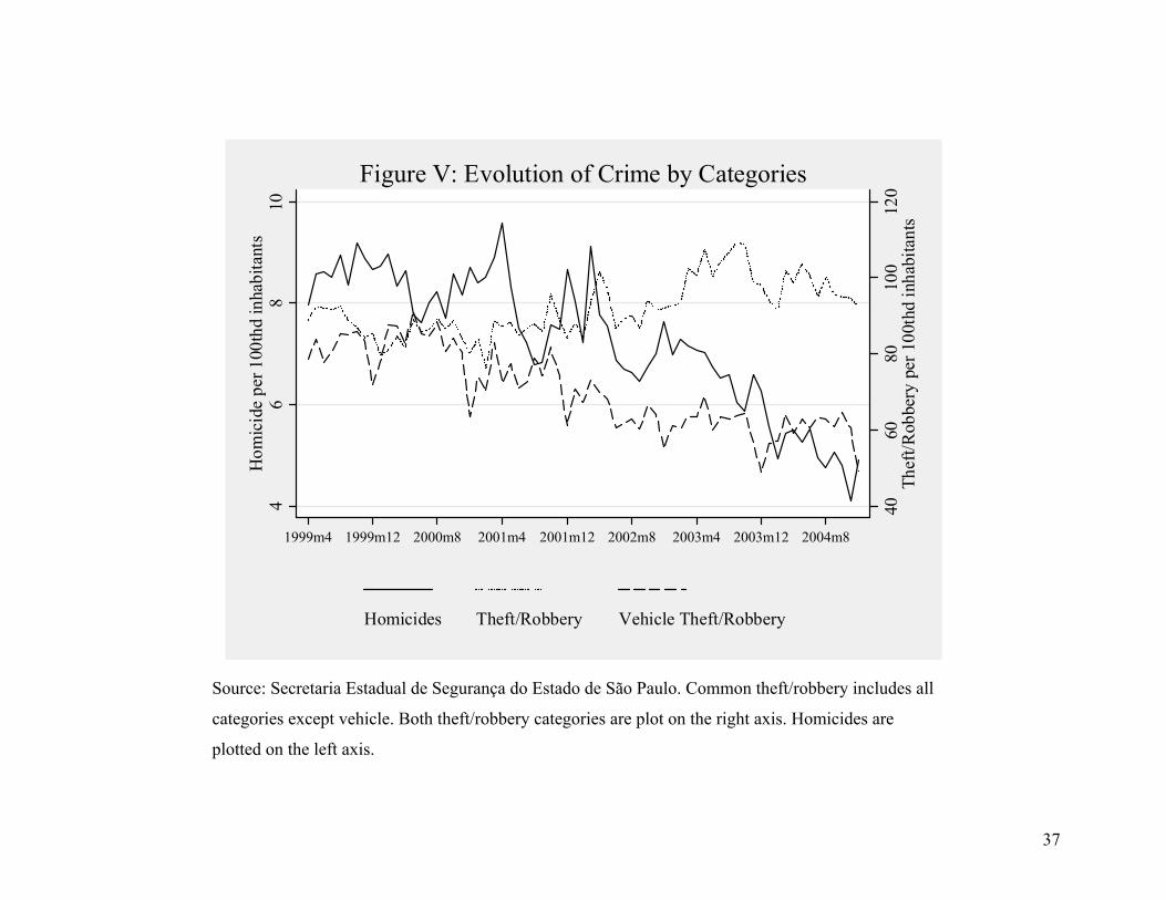
37

4060

8010

012

0Th

eft/R

obbe

ry p

er 1

00th

d in

habi

tant

s

46

810

Hom

icid

e pe

r 100

thd

inha

bita

nts

1999m4 1999m12 2000m8 2001m4 2001m12 2002m8 2003m4 2003m12 2004m8

Homicides Theft/Robbery Vehicle Theft/Robbery

Figure V: Evolution of Crime by Categories

Source: Secretaria Estadual de Segurança do Estado de São Paulo. Common theft/robbery includes all

categories except vehicle. Both theft/robbery categories are plot on the right axis. Homicides are

plotted on the left axis.

38

0

4

8

12

16

20

24

28

32

36

40Pe

rcen

tage

11pm-6am 7am-12am 1pm-6pm 7pm-22pm

Panel A: Vehicle Robbery

0

4

8

12

16

20

24

28

32

36

Perc

enta

ge11pm-6am 7am-12am 1pm-6pm 7pm-22pm

Panel B: Vehicle Theft

SPMA during the years 1999-2003Figure VI: Distribution of Vehicle Theft/Robbery over the Day

Source: Secretaria de Segurança do Estado de São Paulo, INFOCRIM.

39

0

8

16

24

32

40

48Pe

rcen

tage

11pm-6am 7am-12am 1pm-6pm 7pm-10pm

Period 1999-2003Panel A: Bank Robbery

0

8

16

24

32

40

48

Perc

enta

ge11pm-6am 7am-12am 1pm-6pm 7pm-10pm

Period 1999-2003Panel B: Cargo Robbery

City of São PauloFigure VII: Distribution of Robberies over the Day

Source: Secretaria de Segurança do Estado de São Paulo, INFOCRIM.

40

FIGURE VII: Geographical Distribution of Adoption

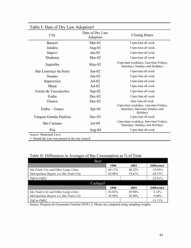
41

Table I: Date of Dry Law Adoption†

City Date of Dry Law Adoption Closing Hours

Barueri Mar-01 11pm-6am all week

Jandira Aug-01 11pm-6am all week

Itapevi Jan-02 11pm-6am all week

Diadema Mar-02 11pm-6am all week

Juquitiba May-02 11pm-6am weekdays, 2am-6am Fridays, Saturdays, Sundays and Holidays

São Lourenço da Serra Jun-02 11pm-6am all week

Suzano Jun-02 11pm-5am all week

Itapecerica Jul-02 11pm-6am all week

Mauá Jul-02 11pm-6am all week

Ferraz de Vasconcelos Sep-02 11pm-6am all week

Embu Dec-02 11pm-5am all week Osasco Dec-02 0am-5am all week

Embu – Guaçu Apr-03 11pm-6am weekdays, 1am-6am Fridays,

Saturdays, 0am-6am Sundays and Holidays

Vargem Grande Paulista Dec-03 11pm-5am all week

São Caetano Jul-04 11pm-6am weekdays, 0am-6am Fridays, Saturdays, Sundays and Holidays

Poá Aug-04 11pm-4am all week Source: Municipal Laws. †: Month the Law was passed in the city council

Table II: Differences in Averages of Bar Consumption as % of Total

Beer 1996 2003 Difference São Paulo City and Other Large Cities 68.17% 48.22% -19.95% Metropolitan Region w/o São Paulo City 62.98% 19.41% -43.57% Diff-in-Diffs‡ -23.61%

Cachaça† 1996 2003 Difference São Paulo City and Other Large Cities 43.82% 45.94% 2.12% Metropolitan Region w/o São Paulo City 45.94% 36.94% -9.00% Diff-in-Diffs‡ -11.11% Source: Pesquisa de Orçamento Familiar (POF). ‡: Means are computed using sampling weights.

42

Dependent Variables:£

(1) (2) (3) (4) (5) (6) (7) (8)In bares In stores In bares In stores

0.326 0.337 0.004 0.078 -7.293 -67.140 92.874 12.847(0.002)*** (0.003)*** (0.003) (0.041) (10.569) (1.596)*** (19.259)** ( 6.770)

0.158 0.199 -0.083 0.217 9.796 -57.725 -34.824 -25.407(0.019)*** (0.030)*** (0.012)** (0.023)** ( 21.766) (13.325)*** (11.825)* (20.294)

-0.640 -0.663 -0.130 -0.185 -121.473 245.583 -119.294 24.466(0.021)*** (0.018)*** (0.012)** (0.052)* (17.875)** ( 11.384)*** (3.981)*** (5.121)**

0.001 0.001 0.447 -0.224 1.859 -0.273(0.001) (0.004) (0.568) (0.429) ( 1.659) (0.215)0.189 0.415 196.802 -22.468 160.430 -29.297

(0.012)*** (0.049)** (42.509)** (19.464) (43.420)* (10.933)0.000 0.001 0.849 0.134 -2.296 -0.626

(0.001) (0.005) (1.105) (0.187) (1.953) (0.313)0.014 0.123 8.441 3.533 68.403 -11.454

(0.011) (0.005)*** (22.854) (1.785) (44.155) (10.089)# Observations 1299 1281 138 138 1281 1281 138 138

R 2 0.066 0.108 0.013 0.243 0.039 0.079 0.125 0.180

£: all estimates are the sub-sample of postive consumptionObservations are weighted using sampling weights

§: Total household consumption of member older than 15 years

Years of Schooling

Age (in years)

Log Income

Gender‡

Source: Pesquisa de Orçamento Familiar (POF). Standard errors clustered at the region level (three regions: City of São Paulo, Metropolitan Region ex City of São Paulo and other large cities) in paretheses.

†: Cachaça is a spirit distilled from sugar cane‡: Gender = 1 if male, 0 = female. Refers to the respondent in the household

*** = significant at the 1% level** = significant at the 5%* = significant at the 10%.

Interaction

Beer Cachaça†

Dummy for 2003

Total Consumption§¥Bar Consumption§ as a % of Total ConsumptionTable III: The Mechanism and Substitution Effects

Dummy for SPMA ex City of São Paulo

Beer Cachaça†

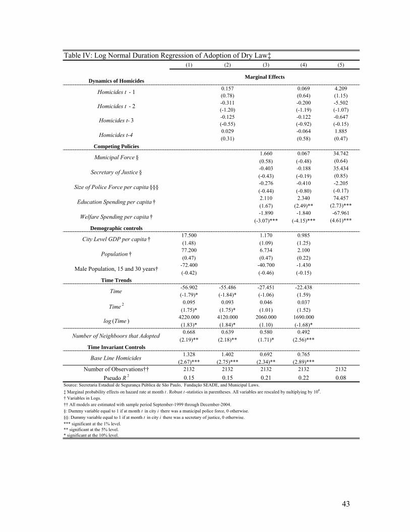
43

(1) (2) (3) (4) (5)

Dynamics of Homicides 0.157 0.069 4.209

(0.78) (0.64) (1.15)-0.311 -0.200 -5.502(-1.20) (-1.19) (-1.07)-0.125 -0.122 -0.647(-0.55) (-0.92) (-0.15)0.029 -0.064 1.885(0.31) (0.58) (0.47)

Competing Policies1.660 0.067 34.742(0.58) (-0.48) (0.64)-0.403 -0.188 35.434(-0.43) (-0.19) (0.85)-0.276 -0.410 -2.205(-0.44) (-0.80) (-0.17)2.110 2.340 74.457(1.67) (2.49)** (2.73)***-1.890 -1.840 -67.961

(-3.07)*** (-4.15)*** (4.61)***Demographic controls

17.500 1.170 0.985(1.48) (1.09) (1.25)77.200 6.734 2.100(0.47) (0.47) (0.22)

-72.400 -40.700 -1.430(-0.42) (-0.46) (-0.15)

Time Trends-56.902 -55.486 -27.451 -22.438(-1.79)* (-1.84)* (-1.06) (1.59)

0.095 0.093 0.046 0.037(1.75)* (1.75)* (1.01) (1.52)

4220.000 4120.000 2060.000 1690.000(1.83)* (1.84)* (1.10) (-1.68)*0.668 0.639 0.580 0.492

(2.19)** (2.18)** (1.71)* (2.56)***Time Invariant Controls

1.328 1.402 0.692 0.765(2.67)*** (2.75)*** (2.34)** (2.89)***

Number of Observations†† 2132 2132 2132 2132 2132Pseudo R 2 0.15 0.15 0.21 0.22 0.08

Table IV: Log Normal Duration Regression of Adoption of Dry Law‡

Marginal Effects

Homicides t - 1

Homicides t - 2

Homicides t- 3

Homicides t-4

Municipal Force §

Secretary of Justice §

Size of Police Force per capita §§§

Education Spending per capita †

Welfare Spending per capita †

City Level GDP per capita †

Population †

Male Population, 15 and 30 years†

Time

Time 2

log (Time )

Number of Neighboors that Adopted

Base Line Homicides

Source: Secretaria Estadual de Segurança Pública de São Paulo, Fundação SEADE, and Municipal Laws.‡ Marginal probability effects on hazard rate at month t . Robust t -statistics in parentheses. All variables are rescaled by nultiplying by 104.† Variables in Logs.†† All models are estimated with sample period September-1999 through December-2004.§: Dummy variable equal to 1 if at month t in city i there was a municipal police force, 0 otherwise.§§: Dummy variable equal to 1 if at month t in city i there was a secretary of justice, 0 otherwise.*** significant at the 1% level.** significant at the 5% level.* significant at the 10% level.

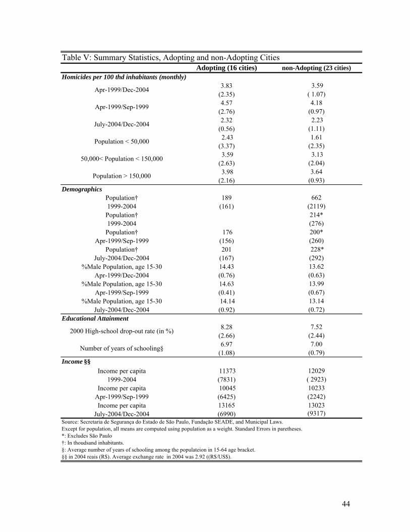
44

Adopting (16 cities) non-Adopting (23 cities)Homicides per 100 thd inhabitants (monthly)

3.83 3.59(2.35) ( 1.07)4.57 4.18

(2.76) (0.97)2.32 2.23

(0.56) (1.11) 2.43 1.61(3.37) (2.35) 3.59 3.13(2.63) (2.04) 3.98 3.64(2.16) (0.93)

DemographicsPopulation† 189 6621999-2004 (161) (2119)

Population† 214*1999-2004 (276)

Population† 176 200*Apr-1999/Sep-1999 (156) (260)

Population† 201 228*July-2004/Dec-2004 (167) (292)

%Male Population, age 15-30 14.43 13.62Apr-1999/Dec-2004 (0.76) (0.63)

%Male Population, age 15-30 14.63 13.99Apr-1999/Sep-1999 (0.41) (0.67)

%Male Population, age 15-30 14.14 13.14July-2004/Dec-2004 (0.92) (0.72)

Educational Attainment8.28 7.52

(2.66) (2.44)6.97 7.00

(1.08) (0.79)Income §§

Income per capita 11373 120291999-2004 (7831) ( 2923)

Income per capita 10045 10233Apr-1999/Sep-1999 (6425) (2242)Income per capita 13165 13023

July-2004/Dec-2004 (6990) (9317)

*: Excludes São Paulo

Table V: Summary Statistics, Adopting and non-Adopting Cities

Source: Secretaria de Segurança do Estado de São Paulo, Fundação SEADE, and Municipal Laws.Except for population, all means are computed using population as a weight. Standard Errors in paretheses.

Apr-1999/Dec-2004

July-2004/Dec-2004

Apr-1999/Sep-1999

Number of years of schooling§

50,000< Population < 150,000

Population < 50,000

Population > 150,000

2000 High-school drop-out rate (in %)

§§ in 2004 reais (R$). Average exchange rate in 2004 was 2.92 ((R$/US$).§: Average number of years of schooling among the populateion in 15-64 age bracket.†: In thoudsand inhabitants.

45

Table VI, Weighted Least Squares† Dependent Variable: Homicides per 100thd inhabitants

(1) (2) (3) (4) -0.642 -0.847 -0.510 -0.490 AdoptLaw (0.346)* (0.361)** (219)*** (0.210)***

Dynamics of Homicide?‡ No No Yes Yes Demographic Controls?‡‡ No No No Yes # Adopting Neighbors?‡‡‡ No No No Yes Competing Policies?‡‡‡‡ No Yes Yes Yes

# Observations 2691 2691 2535 2535 R2 0.529 0.536 0.552 0.552

Source: Secretaria Estadual de Segurança Pública de São Paulo, Fundação SEADE, and Municipal Laws. *** = significant at the 1% level, ** = significant at the 5%, * = significant at the 10%. †: In all specifications, observations are weighted according to population. Standard Errors in parentheses are clustered at the city level, and are thus robust to within city correlation. Period of Analysis is May-1999 through December-2004. All specifications contain a full set of period (month) and city dummies.

‡: 1st, 2nd, 3rd and 4th lags of Homicide per 100thd inhabitants. ‡‡: Logs of population, of income per capita and of the number of 15-30 year-old males. ‡‡‡: Number of bordering cities to city i which at month t that had passed dry laws. ‡‡‡‡: Dummy for the presence in city i at month t of a municipal police force. Dummy for the presence in city i at month t of a municipal secretary of justice. The number of municipal law enforcers per capita: in logs when positive, 0 otherwise; annual variable. Logs of annual spending on education and welfare, both annual.

46

Table VII, Robustness on the Point Estimates† Dependent Variable: Homicides per 100thd inhabitants

OLS Excludes

São Paulo Arellano-

Bond Log of

Homicides City-specific

trends City-specific

trends Placebo

Experiment (1)†† (2) (3)£ (4)₤ (5)§ (6)§ (7)‡

-0.406 -0.679 -0.536 -0.152 -0.602 -0.433 -0.104 AdoptLaw (0.246)* (0.246)*** (0.206)*** (0.059)*** (0.301)** (0.244)* (0.145)

Dynamics of Homicide? Yes Yes Yes Yes No Yes Yes Demographic Controls? Yes Yes Yes Yes Yes Yes Yes # Adopting Neighbors? Yes Yes Yes Yes Yes Yes Yes Competing Policies? Yes Yes Yes Yes Yes Yes Yes

# Observations 2535 2470 2496 1573 2691 2535 2535 R2 0.385 0.492 0.612 0.578 0.571 0.550

Source: Secretaria Estadual de Segurança Pública de São Paulo, Fundação SEADE, and Kahn and Zanetic [2005]. *** = significant at the 1% level, ** = significant at the 5%, * = significant at the 10% †: Weighted Least Squares procedure, unless otherwise noted. Standard Errors in parentheses are clustered at the city level, and are thus robust to within city auto-correlation. Period of Analysis is May-1999 through December-2004. All controls as defined in the legend of table VI. All specifications contain a full set of period (month) and city dummies.

††: OLS procedure, no weighting by population. £: Arellano-Bond GMM procedure, four lags included (p), dependent variable and regressors are first-differences, one-stage standard deviations, Ti - p - 2 lags of the dependent variable used as instruments. No weights included.

₤:Log of Homicide on the dependent variable and the lagged dependent variables. §: One linear trend (θit) for each city i in the sample. City dummies interacted with time. ‡: A placebo experiment: faux treatment dummy (similar for AdoptLaw) that assume the value 1 for adopting cities 12 months before actual adoption.

47

Table VIII, Only Adopting Cities† Dependent Variable: Homicides per 100thd inhabitants

April-1999 to December-

2004

April-1999 to December-

2003

April-1999 to December-

2004

April-1999 to December-

2004 (1) (2) (3)‡ (4)‡

-0.668 -0.804 -0.601 -0.491 AdoptLaw

(0.291)** (0 294)*** (0.293)* (0.287)* Dynamics of Homicide? Yes Yes No Yes Demographic Controls? Yes Yes Yes Yes # Adopting Neighbors? Yes Yes Yes Yes Competing Policies? Yes Yes Yes Yes

# Observations 1040 848 1104 1040 R2 0.524 0.512 0.567 0.549

Source: Secretaria Estadual de Segurança Pública de São Paulo, Fundação SEADE, and Municipal Laws. *** = significant at the 1% level, ** = significant at the 5%, * = significant at the 10%. †: Weighted Least Squares procedure with observations weighted by population. Only adopting cities included. All controls as defined in the legend of table VI. Standard Errors in parentheses are clustered at the city level, and thus robust to within city correlation. Period of Analysis is May-1999 through December-2004, unless otherwise noted. All specifications contain a full set of period (month) and city dummies. ‡: City-specific linear trend included.

Table IX, Summary Statistics: Battery

Adopting (16

cities) non-Adopting (23

cities) Assaults and Battery per 100,000thd inhabitants

27.54 26.78 Jan-2001/Dec-2004 (8.84) (6.99) 27.86 47.08 Population < 50,000

(13.62) (16.41) 28.33 39.11 50,000<Population< 150,000 (9.79) (13.01) 27.20 25.87 Population > 150,000 (8.20) (5.05)

Source: Secretaria de Segurança Pública do Estado de São Paulo and Municipal Laws.

48

Table X: Battery† Dependent Variable: Assault and Battery per 100thd inhabitants

All Sample All Sample All Sample Only Adopters (1) (2) (3) (4)

-4.460 -5.020 -2.915 -1.649 AdoptLaw (2.265)* (1.898)** (0.843)*** (0.719)** Dynamics of Homicide? No No Yes Yes Demographic Controls? No Yes Yes Yes # Neighbors with Law? No Yes Yes Yes

Competing Policies? No Yes Yes Yes # Observations 1872 1872 1716 704

R2 0.702 0.710 0.766 0.656 Source: Secretaria Estadual de Segurança Pública de São Paulo, Fundação SEADE, and Municipal Laws. *** = significant at the 1% level, ** = significant at the 5%, * = significant at the 10%. Observations are clustered at the city level, thus standard errors are robust to within city correlation. All specifications include city and period dummies. Sample is January-2001/December-2004 unless otherwise noted. †: Weighted Least Squares weight = population

Table XI, Summary Statistics: Deaths by Car Accident Adopting (16 cities) non-Adopting (23 cities) Deaths by Car Accidents per 100,000thd inhabitants

0.61 0.55 Apr-1999/Dec-2004 (0.71) (0.33) 0.36 0.25 Population < 50,000

(1.24) (0.92) 0.33 0.27 50,000<Population< 150,000

(0.60) (0.61) 0.73 0.57 Population > 150,000 (0.70) (0.27)

Source: DATASUS and Municipal Laws.

49

Table XII: Deaths in Car Accidents Dependent Variable: Deaths by Car Accidents per 100thd inhabitants

Whole Sample

Largest Adopters and all non-

adopters

Only largest adopters and Non-adopters

(1) (2) (3) -0.055 -0.116 -0.108 AdoptLaw (0.048) (0.053)** (0.071)

Dynamics of Homicide? Yes Yes Yes Demographic Controls? Yes Yes Yes # Adopting Neighbors? Yes Yes Yes Competing Policies? Yes Yes Yes

# Observations 2535 2080 1430 R2 0.360 0.378 0.431

Source: DATASUS, Fundação SEADE, and Municipal Laws. All specifications include a full set of city and period dummies *** = significant at the 1% level, ** = significant 5%, * = significant 10%. Observations are clustered at the city level, thus estimated standard errors are robust to within city correlation

Table XIII, Summary Statistics: Vehicle Robbery Adopting (16 cities) non-Adopting (23 cities) Vehicle Robbery per 100 thd inhabitants (monthly)

24.56 37.81 Apr-1999/Dec-2004 (14.40) (18.55) 17.63 8.76 Population < 50,000 (12.63) (8.54) 20.86 14.27 50,000<Population< 150,000 (17.65) (14.20) 26.27 39.40 Population > 150,000 (12.55) (17.69)

Source: Secretaria de Segurança do Estado de São Paulo and Muncipal Laws. Observations are weighted proportionally to population.

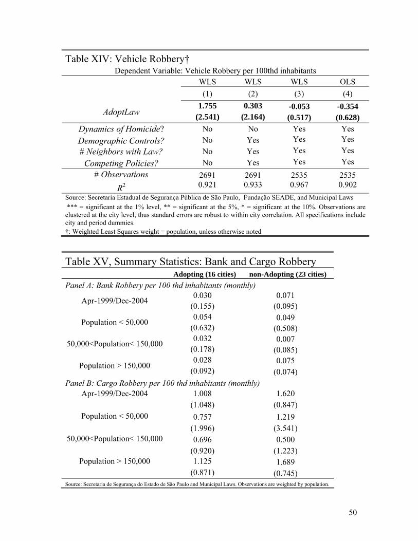
50

Table XIV: Vehicle Robbery† Dependent Variable: Vehicle Robbery per 100thd inhabitants

WLS WLS WLS OLS (1) (2) (3) (4)

1.755 0.303 -0.053 -0.354 AdoptLaw (2.541) (2.164) (0.517) (0.628) Dynamics of Homicide? No No Yes Yes Demographic Controls? No Yes Yes Yes # Neighbors with Law? No Yes Yes Yes

Competing Policies? No Yes Yes Yes # Observations 2691 2691 2535 2535

R2 0.921 0.933 0.967 0.902 Source: Secretaria Estadual de Segurança Pública de São Paulo, Fundação SEADE, and Municipal Laws *** = significant at the 1% level, ** = significant at the 5%, * = significant at the 10%. Observations are clustered at the city level, thus standard errors are robust to within city correlation. All specifications include city and period dummies. †: Weighted Least Squares weight = population, unless otherwise noted

Table XV, Summary Statistics: Bank and Cargo Robbery Adopting (16 cities) non-Adopting (23 cities) Panel A: Bank Robbery per 100 thd inhabitants (monthly)

0.030 0.071 Apr-1999/Dec-2004 (0.155) (0.095) 0.054 0.049 Population < 50,000

(0.632) (0.508) 0.032 0.007 50,000<Population< 150,000

(0.178) (0.085) 0.028 0.075 Population > 150,000 (0.092) (0.074)

Panel B: Cargo Robbery per 100 thd inhabitants (monthly) Apr-1999/Dec-2004 1.008 1.620

(1.048) (0.847) Population < 50,000 0.757 1.219

(1.996) (3.541) 50,000<Population< 150,000 0.696 0.500 (0.920) (1.223)

Population > 150,000 1.125 1.689 (0.871) (0.745) Source: Secretaria de Segurança do Estado de São Paulo and Municipal Laws. Observations are weighted by population.

51

Table XVI: Bank and Cargo Robbery† PANEL A: Dependent Variable: Bank Robbery per 100thd inhabitants

WLS WLS WLS OLS (1) (2) (3) (4)

-0.004 0.016 0.009 0.037 AdoptLaw (0.018) (0.026) (0.028) (0.043) Dynamics of Homicide? No No Yes Yes Demographic Controls? No Yes Yes Yes # Adopting Neighbors? No Yes Yes Yes Competing Policies? No Yes Yes Yes

# Observations 1872 1872 1716 1716 R2 0.207 0.218 0.246 0.225

PANEL B: Dependent Variable: Cargo Robbery per 100thd inhabitants -0.252 0.009 0.034 0.141

AdoptLaw (0.249) (0.152) (0.109) (0.140)

Dynamics of Homicide? No No Yes Yes

Demographic Controls? No Yes Yes Yes

# Adopting Neighbors? No Yes Yes Yes

Competing Policies? No Yes Yes Yes

# Observations 1872 1872 1716 1716 R2 0.581 0.627 0.651 0.338

Source: Secretaria Estadual de Segurança Pública de São Paulo, Fundação SEADE, and Municipal Laws *** = significant at the 1% level, ** = significant at the 5%, * = significant at the 10%. Observations are clustered at the city level, thus standard errors are robust to within city correlation †: Weighted Least Squares weight = population, unless otherwise noted

52

Table XVII, Beggar-thy-Neighbor?† Dependent Variable: Homicides per 100thd inhabitants

Non-adopting and adopting

before adoption

non-adopting and adopting

before adoption

non-adopting and adopting

before adoption

Whole Sample

Population >100,000

Population >200,000 Largest Areas

(1) (2) (3) (4) (5) (6) (7) -0.735 -0.494 -0.604 -0.272 AdoptLaw (0.258)*** (0.207)** (0.284)* (0.130)** 0.238

Interaction (0.204) -0.028 -0.028

# Adopting Neighbors (0.022) (0.048) 0.004

% Adopting Neighbors (0.003)

0.001 % Adopting Neighboring Population (0.002)

Dynamics of Homicide? Yes Yes Yes Yes Yes Yes Yes Demographic Controls? Yes Yes Yes Yes Yes Yes Yes

Competing Policies? Yes Yes Yes Yes Yes Yes Yes # Observations 1495 1495 1495 2535 1365 715 2080

R2 0.631 0.631 0.631 0.572 0.597 0.647 0.564 Source: Secretaria Estadual de Segurança Pública de São Paulo, Fundação SEADE, and Municipal Laws. *** = significant at the 1% level, ** = significant at the 5%, * = significant at the 10%. All controls as defined in the legend of table VI. Period of Analysis is May-1999 through December-2004 unless otherwise noted. Observations are clustered at the city level and thus are robust to within city correlation †: Weighted Least Squares procedure unless otherwise noted.