Embed Size (px)
Citation preview

DSP C5000DSP C5000
Chapter 23Chapter 23
Mobile CommunicationMobile Communication
Speech CodersSpeech Coders
Copyright © 2003 Texas Instruments. All rights reserved.Copyright © 2003 Texas Instruments. All rights reserved.

Copyright © 2003 Texas Instruments. All rights reserved.
ESIEE, Slide 2
OutlineOutline
Speech Coding, CELP CodersSpeech Coding, CELP Coders
Implementation using C54xImplementation using C54x

Copyright © 2003 Texas Instruments. All rights reserved.
ESIEE, Slide 3
Outline – Speech CodingOutline – Speech Coding
Generalities on speech and codingGeneralities on speech and coding Linear Prediction based codersLinear Prediction based coders
Short term and long term predictionShort term and long term prediction Vector QuantizationVector Quantization
CELP codersCELP coders Structure and calculationsStructure and calculations
StandardsStandards

Copyright © 2003 Texas Instruments. All rights reserved.
ESIEE, Slide 4
Applications of Speech CodingApplications of Speech Coding
Digital Transmissions Digital Transmissions On wired telephone:On wired telephone:
MultiplexingMultiplexing Integration of servicesIntegration of services
On wireless channels:On wireless channels: Spectral efficiency Spectral efficiency For better protection against errorsFor better protection against errors
Voice mail/messagingVoice mail/messaging Storage: telephone answering machineStorage: telephone answering machine Secure phoneSecure phone

Copyright © 2003 Texas Instruments. All rights reserved.
ESIEE, Slide 5
Characteristics of CodersCharacteristics of Coders
Bit Rate D: 50 bps < D < 96 kbpsBit Rate D: 50 bps < D < 96 kbps Coding Delay ~ frame delayCoding Delay ~ frame delay Quality Quality
Objective measurements: SNR, PSQMObjective measurements: SNR, PSQM Subjective measurements: MOS Subjective measurements: MOS
(excellent,good,fair,poor,unacceptable)(excellent,good,fair,poor,unacceptable) Intelligibility:Intelligibility:
Objective measure STI or subjective DRTObjective measure STI or subjective DRT Acceptability: E model of ETSI standard, Acceptability: E model of ETSI standard,
communicabilitycommunicability Immunity to noiseImmunity to noise ComplexityComplexity

Copyright © 2003 Texas Instruments. All rights reserved.
ESIEE, Slide 6
Objective Evaluation of the QualityObjective Evaluation of the Quality
The PSQM method:The PSQM method: Objective evaluationObjective evaluation Based on a model of auditive perceptionBased on a model of auditive perception Takes into account the masking effectsTakes into account the masking effects
Good correlation with the MOS grade in Good correlation with the MOS grade in « basic » conditions:« basic » conditions: Low bit rate speech coding, tandem, transmission Low bit rate speech coding, tandem, transmission
errors, ...errors, ...
But sometimes not very reliable :But sometimes not very reliable : Loss of frames, effect of the automatic controlLoss of frames, effect of the automatic control Still under development (PSQM+)Still under development (PSQM+)

Copyright © 2003 Texas Instruments. All rights reserved.
ESIEE, Slide 7
Subjective Evaluation of QualitySubjective Evaluation of Qualityusing the ACR Method yielding MOS scoreusing the ACR Method yielding MOS score A great number of auditors give grades to a A great number of auditors give grades to a
great number of speech sequences. great number of speech sequences. Database with phonetically balanced sentencesDatabase with phonetically balanced sentences Presentation in random orderPresentation in random order Naive auditorsNaive auditors
Statistical processing of results gives the MOS.Statistical processing of results gives the MOS. MOS = Mean OpinionMOS = Mean Opinion Score Score
Bad
Mediocre
Average
Good
Excellent
1
2
3
4
5

Copyright © 2003 Texas Instruments. All rights reserved.
ESIEE, Slide 8
Speech ProductionSpeech Production
Diaphragm
Lungs Larynx
Vocal chords
Nasal Cavity
Mouth Cavity
Palate
Tongue
Lips
Jaws
Vocal tract
Wind Pipe
Articulators
Wind Tunnel
Oscillator

Copyright © 2003 Texas Instruments. All rights reserved.
ESIEE, Slide 9
Speech SignalSpeech Signal

Copyright © 2003 Texas Instruments. All rights reserved.
ESIEE, Slide 10
Speech Spectrum for a Voiced SoundSpeech Spectrum for a Voiced Sound

Copyright © 2003 Texas Instruments. All rights reserved.
ESIEE, Slide 11
Speech Spectrogram Speech Spectrogram
Non stationaryNon stationary Voiced / unvoicedVoiced / unvoiced

Copyright © 2003 Texas Instruments. All rights reserved.
ESIEE, Slide 12
Calculation of SpectrogramsCalculation of Spectrograms
Preac = Preaccentuation, enhances high freqeunciesPreac = Preaccentuation, enhances high freqeuncies
Window = limits the edge effectsWindow = limits the edge effects
Preac Window FFT Log(| |)
Power spectral density
Speech signal
0 2 4 6 8 10 1
2 14 1
6 18 2
0 0
0.1 0.2 0.3 0.4 0.5 0.6 0.7 0.8 0.9 1
Time
Example of window

Copyright © 2003 Texas Instruments. All rights reserved.
ESIEE, Slide 13
Example: Time Signal and SpectrogramExample: Time Signal and Spectrogram
1 2 3 4 5 6 7 80
500
1000
1500
2000
2500
3000
3500
0 1 2 3 4 5 6 7 8 9-3
-2
-1
0
1
2
3x 10
4
TimeTime
FrequencyFrequency
TimeTime
SPECTROGRAMSPECTROGRAM
TIME SIGNALTIME SIGNAL

Copyright © 2003 Texas Instruments. All rights reserved.
ESIEE, Slide 14
Equivalent Electrical ModelEquivalent Electrical Model
NV
V
Stochastic excitation
Periodical excitation
Speech
Spectrum shaping filter
f
Transfer function of the vocal tract
Voicing
Gain
Copyright © 2003 Texas Instruments. All rights reserved.
ESIEE, Slide 15
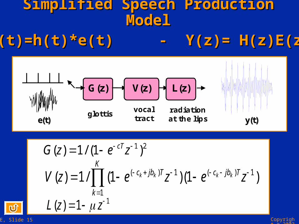
Simplified Speech Production ModelSimplified Speech Production Model
y(t)=h(t)*e(t) - Y(z)= H(z)E(z)y(t)=h(t)*e(t) - Y(z)= H(z)E(z)
V z e z e zc jb T
k
Kc jb Tk k k k( ) / ( )( )( ) ( )
1 1 11
1
1
L z z( ) 1 1
G z e zcT( ) / ( ) 1 1 1 2
G(z) V(z) L(z)
glottis radiation at the lips
vocal tract yy((tt)) ee((tt))

Copyright © 2003 Texas Instruments. All rights reserved.
ESIEE, Slide 16
All Pole Model of the All Pole Model of the Spectrum Shaping FilterSpectrum Shaping Filter
The filter H(z) represents the spectral The filter H(z) represents the spectral envelope since the excitation has a white envelope since the excitation has a white spectrum.spectrum.
1
1 1( ) ( ) ( ) ( ) .
( )1
pi
ii
H z G z V z L zA z
a z

Copyright © 2003 Texas Instruments. All rights reserved.
ESIEE, Slide 17
Short Term Linear PredictionShort Term Linear Prediction
The coefficients of H(z)=1/A(z) can be The coefficients of H(z)=1/A(z) can be obtained by linear prediction.obtained by linear prediction.
Short term analysis on Short term analysis on x(n)x(n) speech signal speech signal Frames of 10 to 30 ms.Frames of 10 to 30 ms.
Least square error criterion:Least square error criterion:
1
2
ˆ( ) ( ) : linear prediction.
ˆ( ) ( ) ( ). criterion: min ( ).
p
ii
n
x n a x n i
e n x n x n e n

Copyright © 2003 Texas Instruments. All rights reserved.
ESIEE, Slide 18
Determination of the Spectral Envelope by Determination of the Spectral Envelope by Linear PredictionLinear Prediction
Prediction Prediction error e(n) = error e(n) = residualresidual is is nearly white, nearly white,
so the spectral envelope of x(n) can be so the spectral envelope of x(n) can be approximated by Sx(f):approximated by Sx(f):
2
2
2
( ) ,( )
is the least square prediction error.
xS fA f
Copyright © 2003 Texas Instruments. All rights reserved.
ESIEE, Slide 19
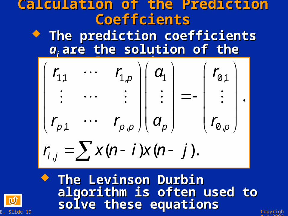
Calculation of the Prediction CoeffcientsCalculation of the Prediction Coeffcients
The prediction coefficients The prediction coefficients aaii are the are the solution of the «normal equations»:solution of the «normal equations»:
1,1 1, 1 0,1
,1 , 0,
,
.
( ) ( ).
p
p p p p p
i j
r r a r
r r a r
r x n i x n j
The Levinson Durbin algorithm is often The Levinson Durbin algorithm is often used to solve these equationsused to solve these equations

Copyright © 2003 Texas Instruments. All rights reserved.
ESIEE, Slide 20
Example of Linear PredictionExample of Linear Prediction
Amplitude of the speech signal
Amplitude of residual signal

Copyright © 2003 Texas Instruments. All rights reserved.
ESIEE, Slide 21
Example of Linear Prediction: Spectral Example of Linear Prediction: Spectral Envelope EstimationEnvelope Estimation
Formants

Copyright © 2003 Texas Instruments. All rights reserved.
ESIEE, Slide 22
Estimation of the Pitch PeriodEstimation of the Pitch Period
Pitch Period TPitch Period T00 estimated by correlation estimated by correlation of the speech signal or residual.of the speech signal or residual. Other methods exist (e.g. cepstrum)Other methods exist (e.g. cepstrum) FF00 = fundamental frequency = 1/T = fundamental frequency = 1/T00
Fractional pitch estimationFractional pitch estimation if the precision if the precision is better than the sampling period.is better than the sampling period.
0
0
50 400
120 160 f 8000 .S
S
Hz F Hz
T kT k i Fs HzT

Copyright © 2003 Texas Instruments. All rights reserved.
ESIEE, Slide 23
Long Term Prediction (LTP)Long Term Prediction (LTP)
The idea is to predict one period of The idea is to predict one period of signal from the preceding one:signal from the preceding one:
ˆ( ) ( ).x n b x n M
2 unknowns: b and M.2 unknowns: b and M.M is the pitch period (when voiced).M is the pitch period (when voiced).
Least square error criterion is used.Least square error criterion is used.

Copyright © 2003 Texas Instruments. All rights reserved.
ESIEE, Slide 24
Long Term Prediction (LTP)Long Term Prediction (LTP)
2n n M n M
n n
b x x x
2
2
n Mn n Mn n
x x x
For a given value of M, optimal b is:For a given value of M, optimal b is:
The best M value maximizes:The best M value maximizes:
All possible values of M must be tested.All possible values of M must be tested.

Copyright © 2003 Texas Instruments. All rights reserved.
ESIEE, Slide 25
Example of Long Term PredictionExample of Long Term Prediction

Copyright © 2003 Texas Instruments. All rights reserved.
ESIEE, Slide 26
LPC 10 VocoderLPC 10 Vocoder
One of the oldest speech coder is the One of the oldest speech coder is the LPC10 vocoder:LPC10 vocoder:The analysis (coder) calculates each The analysis (coder) calculates each
frame:frame:Pitch period, prediction Pitch period, prediction
coefficients, energy, voicing.coefficients, energy, voicing.The synthesis (decoder) uses these The synthesis (decoder) uses these
parameters to synthesize speech from parameters to synthesize speech from the electrical equivalent model.the electrical equivalent model.

Copyright © 2003 Texas Instruments. All rights reserved.
ESIEE, Slide 27
LPC 10 Vocoder (Order 10)LPC 10 Vocoder (Order 10)
Speech frame Linear
Prediction
pitch/voicing
energy
mux
(ai)
E
excitation (600 bps)
Spectrum shaping filter
(1800 bps)
V/UV,F0
CODER
V/UV,F0
E (ai)
1/A(z) Gain
Synthetic speech
Decoder
Frame= 22,5 msFrame= 22,5 ms

Copyright © 2003 Texas Instruments. All rights reserved.
ESIEE, Slide 28
Prediction Spectral ParametersPrediction Spectral Parameters The The aaii coefficients are sensitive to coding and coefficients are sensitive to coding and
interpolation.interpolation. They are replaced by other coefficients:They are replaced by other coefficients:
Reflexion coefficients Reflexion coefficients kkii, log area ratio LARi., log area ratio LARi. Line spectrum frequencies LSFLine spectrum frequencies LSFii..
In the LPC10 vocoderIn the LPC10 vocoder The pitch and voicing are coded on 7 bitsThe pitch and voicing are coded on 7 bits The log of energy on 5 bitsThe log of energy on 5 bits The 10 prediction coefficients ai (transformed in The 10 prediction coefficients ai (transformed in
ki and LARi) are coded on 41 bits.ki and LARi) are coded on 41 bits. A total of 53 bits per frame of 22,5ms = 2400bpsA total of 53 bits per frame of 22,5ms = 2400bps

Copyright © 2003 Texas Instruments. All rights reserved.
ESIEE, Slide 29
Vector Quantization Vector Quantization (2-dimensional example )(2-dimensional example )
k1
k2
-1
-1
1
1
k1
k2
-1
-1
1
1
* *
*
* *
scalar quantization
. . . . . . . . . . . . . . . . .
.
. . . . . . . . .
.
. . . k1
k2
-1
-1
1
1 . .
. . .
. . .
. .
input vectors (training base)
. . . . . . .
vector quantization the index of the code vector is transmitted
Code vector
Bit rate can be decreased by applying VQ to the coefficients.Bit rate can be decreased by applying VQ to the coefficients.

Copyright © 2003 Texas Instruments. All rights reserved.
ESIEE, Slide 30
Line Spectrum Frequencies LSF, LSPLine Spectrum Frequencies LSF, LSP
The Line Spectrum Frequencies fi and The Line Spectrum Frequencies fi and Line spectrum pairs cos(fi) have good Line spectrum pairs cos(fi) have good properties for quantization and properties for quantization and interpolation.interpolation.
The LSF and LSP are derived from the The LSF and LSP are derived from the inverse filter A(z).inverse filter A(z). Build FBuild F11(z) and F(z) and F22(z) symetrical and (z) symetrical and
antisymmetrical polynomials by (for order antisymmetrical polynomials by (for order 10):10):
11 1 11
11 1 12
F ( ) ( ) ( ) /(1 ).
F ( ) ( ) ( ) /(1 ).
z A z z A z z
z A z z A z z

Copyright © 2003 Texas Instruments. All rights reserved.
ESIEE, Slide 31
LSF and LSPLSF and LSP
Roots of FRoots of F11 and F and F2 2 on lie on the unit on lie on the unit circle and are interleaved.circle and are interleaved. 5 conjugate roots exp(j5 conjugate roots exp(jii), f), fii= = ii/(2/(2).).
1 21
1,3,...,9
1 22
2,4,...,10
F ( ) 1 2 .
F ( ) 1 2 .
cos cos 2 . = LSP, = LSP.
ik
ik
i i i i i
z q z z
z q z z
q f q f

Copyright © 2003 Texas Instruments. All rights reserved.
ESIEE, Slide 32
Coders using Short Term and Long Term Coders using Short Term and Long Term Prediction Prediction RELP RELP MPE LP MPE LPCELPCELP
x(n) e(n) r(n)
Calculation of ri,j and ai
Calculation of b and M
Coding of r(n) u(n) B(z) A(z)
Speech signal
residual signal
Analysis
Quantization of coefficients b, M, ai
Quantized coefficients
Quantized residual
u(n) 1/A(z) 1/B(z)
Synthetic speech signal
Synthesis
Quantized coefficients
Quantized residual

Copyright © 2003 Texas Instruments. All rights reserved.
ESIEE, Slide 33
RPE-LTP GSM Full Rate CodersRPE-LTP GSM Full Rate Coders
GSM Full Rate Coder is called:GSM Full Rate Coder is called: RPE LTP= Regular Pulse Excited, Long RPE LTP= Regular Pulse Excited, Long
Term Prediction coderTerm Prediction coder The signal u = the best down-sampled The signal u = the best down-sampled
version (version ( 4) of the residual signal r. 4) of the residual signal r. In CELP coders, vector quantization is In CELP coders, vector quantization is
applied on the signal.applied on the signal. CELP = Code Excited Linear Prediction CELP = Code Excited Linear Prediction
codercoder Each frame of residual signal is compared Each frame of residual signal is compared
to sequences of signal stored in a codebook. to sequences of signal stored in a codebook. The codebook sequences are white and the The codebook sequences are white and the codebook is called stochastic codebook.codebook is called stochastic codebook.

Copyright © 2003 Texas Instruments. All rights reserved.
ESIEE, Slide 34
CELP Coder Basic SchemeCELP Coder Basic Scheme
Analysis by synthesis (closed loop) to Analysis by synthesis (closed loop) to find the best excitation sequence.find the best excitation sequence.
Normalized Stochastic Codebook
1/A(z) 1/B(z) g
-
LS criterion
q
Original speech signal x
Synthetic Speech signal
Copyright © 2003 Texas Instruments. All rights reserved.
ESIEE, Slide 35
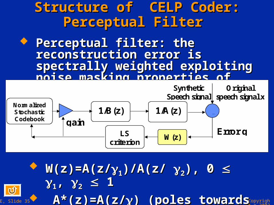
Structure of CELP Coder: Perceptual Filter Structure of CELP Coder: Perceptual Filter
Perceptual filter: the reconstruction error Perceptual filter: the reconstruction error is spectrally weighted exploiting noise is spectrally weighted exploiting noise masking properties of formants.masking properties of formants.
W(z)=A(z/W(z)=A(z/11)/A(z/ )/A(z/ 22), 0 ), 0 11, , 22 1 1 A*(z)=A(z/A*(z)=A(z/) (poles towards zero)) (poles towards zero)
NormalizedStochasticCodebook
1/A(z)1/B(z)gain
-
LScriterion
Error q
Originalspeech signal x
SyntheticSpeech signal
W(z)

Copyright © 2003 Texas Instruments. All rights reserved.
ESIEE, Slide 36
CELP Coder with Perceptual FilterCELP Coder with Perceptual Filter
Original Signal
perceptual Criterion
1/ A(z)
LPC Analysis
Synthetic speech
Iteration on the whole codebook
Gain g
Waveforms codebook
0 1 2
M-1
1/ B(z)
Pitch estimation ana-synt
Search for the best code and gain
W(z) MC
s
s
0 500 1000 1500 2000 2500 3000 3500 0 1 2 3 4 5 6 7 8 9
10
W(f)
1/A(f)

Copyright © 2003 Texas Instruments. All rights reserved.
ESIEE, Slide 37
Basic CELP Structure: Perceptual Filter Basic CELP Structure: Perceptual Filter Inserted in the 2 BranchesInserted in the 2 Branches
Least Square
g
cj
r
Speech frame
H(z) including
g W(z)
W(z)
e
+ -
s Weighted speech frame
Codebook
1/B(z) e
p
s
H(z)=W(z)/A(z)H(z)=W(z)/A(z)

Copyright © 2003 Texas Instruments. All rights reserved.
ESIEE, Slide 38
CELP Structure: Memory of H(z)CELP Structure: Memory of H(z) Memory of H(z) = Output for a zero inputMemory of H(z) = Output for a zero input hhii= impulse response of H(z)= impulse response of H(z)
0
00 1 0known
0
0
( )
ˆ( ) ( ).
ˆ ˆ( ) ( ) ( )
ˆ( ) ( ) ( ).
i n ii
n n
i n i i n i i n ii i n i
p n h e
p n h e h e h e p n
p n p n p n
p n s n p n

Copyright © 2003 Texas Instruments. All rights reserved.
ESIEE, Slide 39
CELP Coder: Memory of H(z)CELP Coder: Memory of H(z)
Least Square
+ -
g
cj
r
Speech frame
p H(z)
includingg W(z)
W(z)
p e
+ -
p0 H(z) Memory
s
1/B(z)
s
Initial conditions equal to zero

Copyright © 2003 Texas Instruments. All rights reserved.
ESIEE, Slide 40
CELP: Adaptive CodebookCELP: Adaptive Codebook LTP can be realized by an adaptive codebookLTP can be realized by an adaptive codebook
0 ( ) 2 1
0 0
ˆ ˆ ˆ ˆ( ) .n n
jn in n i i n i n i M n n
i i
p p h e h gc be p p
1
0
2 ( )
0
ˆ .
ˆ .
n
n i n i Mi
nj
n i n ii
p b h e
p g h c

Copyright © 2003 Texas Instruments. All rights reserved.
ESIEE, Slide 41
CELP with Stochastic CodebookCELP with Stochastic Codebook
Least Square
+ -
g 1
g 2
c 1,i(0)
c 2,i(1)
Speech frame
p H(z)
W(z)
p e
+ -
p0
H filter memory
s
H(z)
p1
p2
Adaptive codebook
Stochastic codebook
The adaptive codebook stores the past residual frames. It is called The adaptive codebook stores the past residual frames. It is called adaptive because its content changes with timeadaptive because its content changes with time..

Copyright © 2003 Texas Instruments. All rights reserved.
ESIEE, Slide 42
CELP DecoderCELP Decoder
g 1
g 2
c 1,i(0)
c 2,i(1)
Synthetic speech 1/A(z)
Adaptive codebook
Stochastic codebook
Decode received parameters: Index of stochastic codebook Gain of stochastic codebook Index of adaptive codebook Gain of adaptive codebook Linear prediction filter coefficients

Copyright © 2003 Texas Instruments. All rights reserved.
ESIEE, Slide 43
CELP Equations CELP Equations Example: Searching through CodebooksExample: Searching through Codebooks
The main load is the filtering of all the The main load is the filtering of all the codebook vectors.codebook vectors.
c j,i(j) H(z)
Nul Initial conditions
f j,i(j)
jth Filtered codebook
jth Original codebook
, ( ) , ( ) , ( )
, ( ) , ( ) , ( ) , ( )0
ˆ . ( ) ( )* ( ).
( ) ( ) ( ). .
j j i j j i j j i j
n
j i j j i j j i j j i jk
g f n h n c n
f n h k c n k
jp f
f Hc

Copyright © 2003 Texas Instruments. All rights reserved.
ESIEE, Slide 44
Filtering Matrix HFiltering Matrix H
0
1 0
2 1 0
1 2 1 0
0 0
0
0
0
N
h
h h
H h h h
h h h h
H(n) is the impulse response H(n) is the impulse response corresponding to H(z).corresponding to H(z).
N = length of the codebook vectors.N = length of the codebook vectors.

Copyright © 2003 Texas Instruments. All rights reserved.
ESIEE, Slide 45
Finding the Best Excitation in the Coder:Finding the Best Excitation in the Coder:Equation of the SolutionEquation of the Solution
J least square criterionJ least square criterion For a set of 2 vectors For a set of 2 vectors ccj,i(j)j,i(j), F is the 2 , F is the 2
column matrix of filtered vectors column matrix of filtered vectors ffj,i(j)j,i(j)
2 2
2 1
ˆ
Optimal gain:
ˆmin max ( )
T T
T T T
J p p p Fg
F F g F p
J p p F F F F p

Copyright © 2003 Texas Instruments. All rights reserved.
ESIEE, Slide 46
CELP Optimal SolutionCELP Optimal Solution
Optimal algorithm finds the best Optimal algorithm finds the best combination of code vectors maximizing combination of code vectors maximizing the norm and finds the optimal gains the norm and finds the optimal gains ggjj..
But the number of combinations of But the number of combinations of codebook vectors is very high and the codebook vectors is very high and the complexity is also great. Example:complexity is also great. Example: M=1024 for the stochastic codebookM=1024 for the stochastic codebook and M=256 for the adaptive codebookand M=256 for the adaptive codebookLeads to 262 144 solutions to test andLeads to 262 144 solutions to test and1280 vectors to filter.1280 vectors to filter.

Copyright © 2003 Texas Instruments. All rights reserved.
ESIEE, Slide 47
Iterative Suboptimal Algorithm for 2 Iterative Suboptimal Algorithm for 2 CodebooksCodebooks
First step:First step: Target vector = pTarget vector = p Find the best vector in the adaptive Find the best vector in the adaptive
codebook and its gain.codebook and its gain. Calculate the new target vector p1:Calculate the new target vector p1:
11 ˆn np p p
Second step: Second step: Target vector = p1Target vector = p1Find the best vector in the stochastic Find the best vector in the stochastic
codebook and its gain.codebook and its gain.

Copyright © 2003 Texas Instruments. All rights reserved.
ESIEE, Slide 48
Iterative AlgorithmIterative Algorithm
-
H(z)
W(z)
p2 g2
p0
Speech
c(n,j)
j,g1
H(z) p1 g1 e(n-M)
LSS
M,g2
+ g1
g2
p
p1
LSS

Copyright © 2003 Texas Instruments. All rights reserved.
ESIEE, Slide 49
Operations of the Iterative AlgorithmOperations of the Iterative Algorithm
At step j, the optimal codebook vector At step j, the optimal codebook vector has index i:has index i:
2 2
,ˆarg min =j j j j j kk
i g p p p f
, ,opt,
, , , ,
.T Tj j k j j k
k T Tj k j k j k j k
g T
p f p Hc
f f c H Hc
22
opt,, ,
arg max with Tj j k k
kT Tkj k j k k k
i g
p Hc
c H Hc

Copyright © 2003 Texas Instruments. All rights reserved.
ESIEE, Slide 50
Iterative AlgorithmIterative Algorithm
Numerical Example :Numerical Example : FFSS=8000Hz,=8000Hz, M=256 size of the stochastic codebookM=256 size of the stochastic codebook MMaa=128 size of the adaptive codebook=128 size of the adaptive codebook Frame size NFrame size NTT=160, 20ms=160, 20ms Frames split in 4 subframes of N=40 samplesFrames split in 4 subframes of N=40 samples p=10 linear prediction orderp=10 linear prediction order 10 Mips to filter the stochastic codebook.10 Mips to filter the stochastic codebook.

Copyright © 2003 Texas Instruments. All rights reserved.
ESIEE, Slide 51
Iterative AlgorithmIterative Algorithm
The main processing load is the filtering The main processing load is the filtering of the codebooks vectors.of the codebooks vectors.
Many algorithms have been proposed to Many algorithms have been proposed to decrease the computation load:decrease the computation load: Special structures of the codebook:Special structures of the codebook:
VSELP: Vector SumVSELP: Vector Sum Algebraic codebook: ACELPAlgebraic codebook: ACELP Linear codebook (the adaptive codebook is Linear codebook (the adaptive codebook is
linear).linear).
Structure of H avoidStructure of H avoidiing the filtering:ng the filtering: Diagonalization of HDiagonalization of HTTHH

Copyright © 2003 Texas Instruments. All rights reserved.
ESIEE, Slide 52
CELP CodingCELP Coding
Standards from 4.8 kbps to 16 kbpsStandards from 4.8 kbps to 16 kbps Federal standard (DOD) (4.8 kbps)Federal standard (DOD) (4.8 kbps)
frame = 260 samples (30 ms)frame = 260 samples (30 ms) LPC 8 --> (LSP coding 34 bits)LPC 8 --> (LSP coding 34 bits) adaptive codebook (256 vectors (fractional adaptive codebook (256 vectors (fractional
pitch))pitch)) stochastic codebook (512 vectors (-1,0,1))stochastic codebook (512 vectors (-1,0,1))

Copyright © 2003 Texas Instruments. All rights reserved.
ESIEE, Slide 53
VSELP (Vector Sum Excitation Coding)VSELP (Vector Sum Excitation Coding)
Codebook vectors v are combinations of Codebook vectors v are combinations of basis vectors (b1,b2,...,bk) basis vectors (b1,b2,...,bk) v=+/- b1 +/- b2 +/- ... +/- bkv=+/- b1 +/- b2 +/- ... +/- bk
Only the basis vectors are filteredOnly the basis vectors are filtered Motorola ( 8 kbps)Motorola ( 8 kbps) GSM (half rate)(5.6 kbps)GSM (half rate)(5.6 kbps)

Copyright © 2003 Texas Instruments. All rights reserved.
ESIEE, Slide 54
Fractional PitchFractional Pitch The precision of the pitch period is a fraction of The precision of the pitch period is a fraction of
sample Tsample TSS. An interpolation filter is used.. An interpolation filter is used. B(z)=1-bz-B(z)=1-bz-MM
ff with M with Mff=M+ =M+ x(n-M-x(n-M-) can be written as:) can be written as:
TFTF-1-1(X(f)*e(X(f)*e(-j2(-j2f(M+f(M+)Te))Te))) = x(n-M)* TF= x(n-M)* TF-1-1(e(e(-j2(-j2ffTe)Te)) =x(n-M)* h(n)) =x(n-M)* h(n)
h(n)sinc((n-))
+Fe/2 -Fe/2 f
| H(f)|
Interpolation filter H H(f)
0 2 4 6 8 10 12 14 -0.5
0
0.5
1
=1/4 T S
Time in TS

Copyright © 2003 Texas Instruments. All rights reserved.
ESIEE, Slide 55
StandardsStandards
Rate (Kbits/s) 1k 2k 4k 16k 32k 64k
Quality MOS
Production model
Hybrid coders Waveform coding
1
2
3
4
5 G711 (72)
G721 (84)
ST4209 (83)
G728 (92)
(90)
G729 (96)
ST4479 (93)
ST 4198
(87)
2400 HSX (96)
LPC 10 (83)
GSM (87)
1200 HSX
(97)
G723-1 (96)
0,5k
Langage model
8k
FS1016

Copyright © 2003 Texas Instruments. All rights reserved.
ESIEE, Slide 56
StandardsStandards Wired Telephony UIT-T Wired Telephony UIT-T
G 711 (1972)G 711 (1972) : PCM: PCM 64 kbps64 kbps G 721 (1984)G 721 (1984) : ADPCM: ADPCM 32 kbps32 kbps G 728 (1991)G 728 (1991) : LD_CELP: LD_CELP 16 kbps 16 kbps G 729G 729 : CS-ACELP: CS-ACELP 8 kbps 8 kbps
Mobile communications (ETSI - CTIA)Mobile communications (ETSI - CTIA) GSM (FR ) GSM (FR ) :RPE_LTP :RPE_LTP 13 kbps13 kbps GSM (HR) GSM (HR) :VSELP:VSELP 5.6 kbps5.6 kbps GSM (EFR) GSM (EFR) : ACELP : ACELP 12.2 kbps12.2 kbps UMTS (AMR) : ACELPUMTS (AMR) : ACELP 12.2 to 4.75 Kbps12.2 to 4.75 Kbps
Military applications (NATO)Military applications (NATO) FS 1015 (1976)FS 1015 (1976) : LPC10: LPC10 2.4 kbps2.4 kbps FS 1016 (1991)FS 1016 (1991) : CELP: CELP 4.8 kbps4.8 kbps

Copyright © 2003 Texas Instruments. All rights reserved.
ESIEE, Slide 57
AMR Adaptive MultiRate Coder AMR Adaptive MultiRate Coder for 3G Applicationfor 3G Application
8 Narrow Band NB AMR source coders8 Narrow Band NB AMR source coders 12.2 10.2 7.95 7.40 6.70 5.90 5.15 4.75 kbps12.2 10.2 7.95 7.40 6.70 5.90 5.15 4.75 kbps
9 Wide Band coders WB AMR coders9 Wide Band coders WB AMR coders Based on ACELPBased on ACELP Frame of 20 ms, fs=8000 HzFrame of 20 ms, fs=8000 Hz

Copyright © 2003 Texas Instruments. All rights reserved.
ESIEE, Slide 58
IUT Civil StandardsIUT Civil Standards
UIT Standard
Method YearBit rate in
KbpsDelay in ms
Quality MOS
Complexity in Mips
G711 PCM 1972 64 0.125 4.3 <<1
G721 ADPCM 1984 32 0,1254.1 at
32Kbps1.25
G723 1986 40-32-24G726 1988 40-32-24-16G727 1990 40-32-24-16G728 LD-CELP 1992 16 2.5 4.0 30G729 CS-ACELP 1994 8 30 3.9 25
G729a 1996 12
G723.1MP-MLQ ACELP
1995 6.3 5.3 75 3.9 24

Copyright © 2003 Texas Instruments. All rights reserved.
ESIEE, Slide 59
ETSI and Inmarsat StandardsETSI and Inmarsat Standards
Inmarsat Standard
Method YearBit rate in
KbpsDelay in ms
Quality MOS
Complexity in Mips
IMBE IMBE 1990 4.15 78.75 3.4 7Mini-M AMBE 1995 3.6 3.6 25
Standard ETSI
europeMethod Year
Bit rate in Kbps
Delay in msQuality
MOSComplexity
in Mips
GSM RPE-LTP 1987 13 40 3.47 6TETRA ACELP 1994 4.567 67.5 12
GSM HR VSELP 1994 5.6 45 30EFR-GSM (identical
DCS)ACELP 1995 12.8 40 15

Copyright © 2003 Texas Instruments. All rights reserved.
ESIEE, Slide 60
TIA and RCR StandardsTIA and RCR Standards
TIA standard
USAMethod Year
Bit rate in Kbps
Delay in msQuality
MOSComplexity
in Mips
IS54 VSELP 1989 7.95 45 3.5 20IS96 QCELP 1993 8.5-4.2-0.8 45 4 20
IS136 ACELP 1995 7.4 45IS127 EVRC RCELP 1995 8.5-4-0.8 >45 20PCS 1900 ACELP 1995 40 15
TIA standard
USAMethod Year
Bit rate in Kbps
Delay in msQuality
MOSComplexity
in Mips
RCR STD-27B
VSELP 1990 6.7 45 20
JDC HR PSI-CELP 1993 3.45 90 50

Copyright © 2003 Texas Instruments. All rights reserved.
ESIEE, Slide 61
Implementation of CELP Coders on C54xImplementation of CELP Coders on C54x
Example of the G729 Annex A.Example of the G729 Annex A. Specific instruction for codebook search Specific instruction for codebook search Some functions of DSPLIBSome functions of DSPLIB

Copyright © 2003 Texas Instruments. All rights reserved.
ESIEE, Slide 62
Profiling Example for G729 Annex AProfiling Example for G729 Annex A using C Compiler using C Compiler
G729 is a CS-ACELP Coder (ITU 1995)G729 is a CS-ACELP Coder (ITU 1995) 8Kbps with quality of ADPCM at 8Kbps with quality of ADPCM at
32Kbps G726. 32Kbps G726. DSVD: G729 Annex A voice over DSVD: G729 Annex A voice over
internet, voice e-mailinternet, voice e-mail Digital Simultaneous Voice & DataDigital Simultaneous Voice & Data
Copyright © 2003 Texas Instruments. All rights reserved.
ESIEE, Slide 63
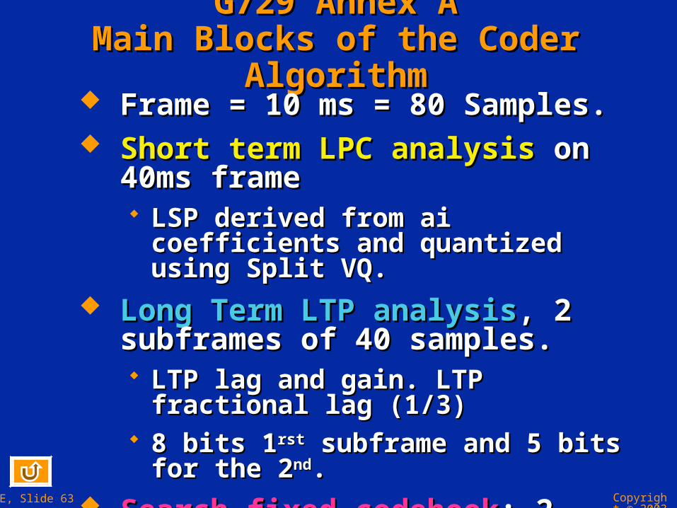
G729 Annex AG729 Annex AMain Blocks of the Coder AlgorithmMain Blocks of the Coder Algorithm Frame = 10 ms = 80 Samples.Frame = 10 ms = 80 Samples. Short term LPC analysisShort term LPC analysis on 40ms frame on 40ms frame
LSP derived from ai coefficients and LSP derived from ai coefficients and quantized using Split VQ.quantized using Split VQ.
Long Term LTP analysisLong Term LTP analysis, 2 subframes , 2 subframes of 40 samples. of 40 samples. LTP lag and gain. LTP fractional lag (1/3)LTP lag and gain. LTP fractional lag (1/3) 8 bits 18 bits 1rstrst subframe and 5 bits for the 2 subframe and 5 bits for the 2ndnd..
Search fixed codebookSearch fixed codebook: 2 subframes of : 2 subframes of 40 samples. Index and gains40 samples. Index and gains Code length = 40 with 4 non-zero pulses Code length = 40 with 4 non-zero pulses 1.1.

Copyright © 2003 Texas Instruments. All rights reserved.
ESIEE, Slide 64
Structures of Frames Structures of Frames
Previous speech 120
Subframe 1 40
Subframe 2 40
Next frame 40
Present frame, 80 samples = L_Frame
New speech, 80 samples = L_Frame
Total speech vector, 240 samples = L_Total
LPC analysis window, 240 samples = L_Window

Copyright © 2003 Texas Instruments. All rights reserved.
ESIEE, Slide 65
G729 Annex A, Bit AllocationG729 Annex A, Bit Allocation
Total in bits1818131
2681480
1rst subframe (5ms) in bits
2nd subframe (5ms) in bits
LPC filter
pitch period parity check
Fixed codebookPulse positions
Pulse signsCodebook gains
81
7 = 3+44
Adaptive codebook:
7 = 3+4
13 = (3x3+4)
5
13 = (3x3+4)4

Copyright © 2003 Texas Instruments. All rights reserved.
ESIEE, Slide 66
G729 Annex AG729 Annex AMain Blocks of the Decoder AlgorithmMain Blocks of the Decoder Algorithm
The serial received bits are converted into The serial received bits are converted into parameters:parameters: LSP vector, 2 fractional pitch lags and gains, 2 LSP vector, 2 fractional pitch lags and gains, 2
fixed codebook index and gains.fixed codebook index and gains.
LSP are converted to LP filter coefficients LSP are converted to LP filter coefficients ai and interpolated at each subframe.ai and interpolated at each subframe.
At each subframe:At each subframe: The excitation is constructed and scaled.The excitation is constructed and scaled. The speech is synthesized by filtering the The speech is synthesized by filtering the
excitation by the LP synthesis filter.excitation by the LP synthesis filter.
Postprocessing by an adaptive postfilter.Postprocessing by an adaptive postfilter.

Copyright © 2003 Texas Instruments. All rights reserved.
ESIEE, Slide 67
Using the C CompilerUsing the C Compiler Use the C program of the standard and C Use the C program of the standard and C
compiler with maximum optimization.compiler with maximum optimization. Autocorrelation Autocorrelation = 488 445 cycles= 488 445 cycles Levinson Levinson = 164 843 cycles= 164 843 cycles Conversion ai LSFConversion ai LSF = 410 404 cycles= 410 404 cycles LSF Quantization LSF Quantization = 883 853 cycles= 883 853 cycles Synthesis filteringSynthesis filtering = 501 472 cycles= 501 472 cycles Pitch open loopPitch open loop = 793 533 cycles= 793 533 cycles Fractional PitchFractional Pitch = 2 x 618 354 cycles= 2 x 618 354 cycles Search Algebraic codeSearch Algebraic code = 2x 617 582 cycles= 2x 617 582 cycles Gains quantizationGains quantization = 2x 10⁸ 480 = 2x 10⁸ 480
cyclescycles

Copyright © 2003 Texas Instruments. All rights reserved.
ESIEE, Slide 68
Assembly Language Instructions for Assembly Language Instructions for Codebook SearchCodebook Search
Better results can be obtained with Better results can be obtained with assembly language than C.assembly language than C.
Specific instructions for codebook Specific instructions for codebook search: search: Conditional storesConditional stores..
CodeBook Search (Conditional Stores) STRCD Xmem, cond SRCCD Xmem, cond SACCD src, Xmem, cond
Xmem = T if condition is true Xmem = BRC if condition is true Xmem = src if condition is true
STRCD = Store T Conditionally SRCCD = Store Block Repeat Counter Conditionally SACCD = Store Accumulator Conditionally

Copyright © 2003 Texas Instruments. All rights reserved.
ESIEE, Slide 69
Assembly Language Codebook SearchAssembly Language Codebook Search
2 2i
Best code book index
carg max noted find max of
G
opt
iopt
ii i
j
j
222 2
To avoid division:
.optii opt opt i
i opt
ccc G c G
G G

Copyright © 2003 Texas Instruments. All rights reserved.
ESIEE, Slide 70
Assembly Language Codebook SearchAssembly Language Codebook Search .mmregs .text CBS: STM #C, AR5 STM #G, AR2 STM #G-opt, AR3 STM #I-opt, AR4 ST #0, *AR4 ST #1, *AR3+ ST #0, *AR3- STM #N-1, BRC RPTBD done SQUR *AR5+, A MPYA *AR3+ MAS *AR2+, *AR3-, B SRCCD *AR4, BGEQ STRCD *AR3+, BGEQ SACCD A, *AR3-, BGEQ
SQUR *AR5+, A done: MPYA *AR3+
AR5 C(0) ...
AR3 Gopt=1 Copt2=0
AR4 Iopt=0
AR2 G(0) ...
A=C(i)A=C(i)22
B=B= C(i)C(i)22Gopt T=GoptGopt T=Gopt B=B= C(i)C(i)22Gopt-G(i)CoptGopt-G(i)Copt22
If (B If (B 0) then: 0) then: BRC BRC
GoptGopt T T Iopt Iopt A A
CoptCopt22