David Taylor Research CenterBethesda, Maryland 20084-5000

AD-A241 208

DTRC / SHD-1350-01 March 1991

Ship Hydromechanics Department D TiCS -L !:CT E

SEP 2 41991

D UA MATHEMATICAL MODEL FOR SURFACE SHIP MANEUVERING

by

William R. McCreight

E

- 91-11291

6

o

Cn Approved for Public Released: Distribution is Unlimited

9'2 91-12

i I~ l il ill I lt- I

CODE 011 DIRECTOR OF TECHNOLOGY, PLANS AND ASSESSMENT

12 SHIP SYSTEMS INTEGRATION DEPARTMENT

14 SHIP ELECTROM1"GIAGNETIC SIGNATURES DEPARTMENT

15 SHIP HYDROMECHANICS DEPARTMENT

16 AVIATION DEPARTMENT

17 SHIP STRUCTURES AND PROTECTION DEPARTMENT

18 COMPUTATION, MATHEMATICS & LOGISTICS DEPARTMENT

19 SHIP ACOUSTICS DEPARTMENT

27 PROPULSION AND AUXILIARY SYSTEMS DEPARTMENT

28 SHIP MATERIALS ENGINEERING DEPARTMENT

DTRC ISSUES THREE TYPES OF REPORTS:

1. DTRC reports, a formal series, contain information of permanent technical value.They carry a consecutive numerical identification regardless of their classification or theoriginating department.

2. Departmental reports, a semiformal series, contain information of a preliminary,temporary, or proprietary nature or of limited interest or significance. They carry adepartmental alphanumerical identification.

3. Technical memoranda, an informal series, contain technica! documentation oflimited use and interest. They are primarily working papers intended for internal use. Theycarry an identifying number which indicates their type and the numerical code of theoriginating department. Any distribution outside DTRC must be approved by the head ofthe originating department on a case-by-case basis.

- UNCLASSIFIEDSECURITY CLASSIFICATION OF THIS PAGE

REPORT DOCUMENTATION PAGE"a. REPORT SECURITY CLASSIFICATION lb. RESTRICTIVE MARKINGS

Unclassified2a. SECURITY CLASSIFICATION AUTHORITY 3. DISTRIBUTION / AVAILABILITY OF REPORT

Approved for Public Release2z DECLASSIFICATION /DOWNGRADING SCHEDULE Distribution is Unlimited

PERFORMING ORGANIZATION REPORT NUMBER(S) 5. MONITORING ORGANIZATION REPORT NUMBER(S)

DTRC / SHD-1350-01

Ea NAME OF PERFORMING ORGAN;ZATION 6b. OFFICE SYMBOL 7a NAME OF MONITORING ORGANIZATION

David Taylor Research Center i Naval Sea Systems Command1 1562 _6C ADDRESS (City, State, and Zip Coda) Tb. ADDRESS (Ciy, State, and Zip Code)

Bethesda, MD 20084-5000 Washington, D.C. 20362

aa. NAME OF FUNDING / SPONSORING 8b, OFFICE SYMBOL 9. PROCUREMENT INSTRUMENT IDENTIFICATION NUMBERORGANIZATION (f ppicabte )

Naval Sea Systems Command SEA 55W3

8c. ADDRESS (City, State, and Zip Code) 10. SOURCE OF FUNDING NUMBERS

PROGRAM PROJECT TASK WORK UNITWashington, D.C. 20362 ELEMENT NO. NO. NO. ACCESSION NO.

24313N I DN508317

11. TITLE (Indude Security Ciassication)

A Mathematical Model for Surface Ship Maneuvering

12. PERSONAL AUTHOR(S)William R. McCreight

13a. TYPE OF REPORT 13b. TIME COVERED 14. DATE OF REPORT (YeW, Month, Day) 15. PAGE COUNT

Final I FROM TO 1991 March 2416. SUPPLEMENTARY NOTATION

17. COSATI CODES 18. SUBJECT TERMS (Connue on reveme i fnecasary and Identify by bock number)

FIELD GROUP SUB-GROUP Maneuvering

19. ABSTRACT (Continue on reverse if necessary and Identit1 by block number)

The mathematical model for a time domain simulation of a surface ship maneuvering in calm water ispresented. The six-degree-of-freedom mathematical model is applicable to conventional monohuls orSWATHs. Included are calm water hydrodynamic forces, hydrostatic forces, unsteady wind forces,slowly-varying wave drift forces, and forces due to a towed body. The model depends upon data derivedfrom model experiments. This model represents an improvement over previous models in several respects.Most notable are the changes in the modeling of resistance, calm water surge hydrodynamic forces, andpropeller-rudder interaction which together lead to improved speed loss prediction.

20 DISTRIBL;TION / AVAILABILITY OF ABSTRACT 21. ABSTRACT SECURITY CLASSIFICATION

0 UNCLASS1FIED/UNUMrTED [I] SAME AS RPT 0 DIC USERS Unclassified2a. NAME OF RESPONSIBLE INDIVIDUAL 22b. TELEPHONE (include Arse Code) 22c. OFFICE SYMBOL

William R. McCreight (301) 227-1720 1561

DD FORM 1473, 84 MAR 53 APR ediion may be Used unil exhausted SECURITY CLASSIFICATION OF THIS PAGE

A ,ot ., ,4400 or* UNCLASSIFIEDi

UNCLASSIFIEDSECURITY CLASSIFICATION OF THIS PAGE

UNCLASSIFIEDSECURITY CLASSFICATION OF THIS PAGE

ii

CONTENTS

page

ABSTRACT ................................................................................................................................... 1

ADM IN ISTRATIVE IN FORM ATION ....................................................................................... I

IN TRO DUCTIO N .......................................................................................................................... 1

EQUATION S OF M OTION .................................................................................................... 4

COO RDIN ATE SYSTEM S ............................................................................................. 4

DYN AM ICS ...................................................................................................................... 4

EXTERN AL FORCES AN D M OM ENTS ..................................................................................... 6

HYDROSTATIC FORCES ............................................................................................. 6

CALM W ATER HYDRODYN AM IC FORCES ................................................................ 7

Resistance and Propulsion Model .......................................... 9

M achinery M odel .............................................................................................. 11

W IN D FORCES ................................................................................................................. 12

Unsteady W ind M odel ....................................................................................... 12

Approxim ation for W ind Force Coefficients ....................................................... 13

W AVE FORCES ................................................................................................................. 14

Slowly-Varying W ave Drift Force M odel .......................................................... 16

TOW FORCES ................................................................................................................... 17

SOLUTION OF THE EQUATION S OF M OTION ...................................................................... 18

CON CLUSION .............................................................................................................................. 19

APPENDIX - ADDITIONAL TERMS IN WAVMAN44 OR TOWMAN87 ....................... 21

REFEREN CES ................................................................................................................................ 23

"DT'O T,-K,,

Diti ';tio .I

Av L, .

Di- t i>

iii

ABSTRACT

The mathematical model for a time domain simulation of a surfaceship maneuvering in calm water is presented. The six-degree-of-freedom mathematical model is applicable to conventionalmonohulls or SWATHs. Included are calm water hydrodynamicforces, hydrostatic forces, unsteady wind forces, slowly-varying wavedrift forces, and forces due to a towed body. The model depends upondata derived from model experiments. This model represents animprovement over previous models in several respects. Most notableare the changes in the modeling of resistance, calm water su:gehydrodynamic forces, and propeller-rudder interaction whichtogether lead to improved speed loss prediction.

ADMINISTRATIVE INFORMATION

I his report was funded by Program Element 24313N, D N Number DN 508317 and Work

Unit Number 1-1235-985

INTRODUCTION

This report documents the current state of a time domain simulation for the

maneuvering of surface ships, including the effect of unsteady wind forces (wind gusts), slowly-

varying wave drift forces in long- or short-crested seas, and forces due to a towed body. This

model is suitable for trackkeeping studies as well as traditional maneuverability studies. It

has evolved at the David Taylor Research Center (DTRC) over a period of more than two

decades from the original three-degree-of-freedom model of Strom-Tejsen[1], based on the

mathematical model of Abkowitz[2]. Many people have worked on it, or influenced its

development.

Motterl added a fourth degree of freedom (roll) and the propeller and rudder model of

Smit and Chislett [3]. McCreight and Motter1 carried out a major rewrite of this program as the

first stage of an effort to develop a full maneuvering in waves model. In addition to structuring

the program, a steady wind model was added, coefficients were added to be valid over an

extended speed range instead of merely accounting for "small" deviations from the initial

conditions, improved roll damping. Provision was made for defining an arbitrary sequence of

rudder and speed commands. A nonlinear initialization scheme was developed to handle the

large excursions which can be caused by strong winds. Finally, the previously used Euler

integration was replaced by an adaptive Runge-Kutta which allowed the use of large step sizes

1 Published in reports with limited distribution.

while maintaining accuracy. This was particularly important due to the sensitivity of the

model in roll. In addition, a detailed model of steam turbine, gas turbine, and diesel engines

was incorporated by Propulsion Dynamics, Inc. (PDI)[4]. PDI also produced a user's manual for

this program. This maneuvering program was known as WAVMAN44 for historical reasons,

even though it has no wave effects. WAVMAN44 has been used in many maneuvering studies,

and has been the base for two further developments.

The first and most extensive of the developments is the originally planned

maneuvering in waves simulation, which added two additional degrees of freedom (heave and

pitch) to produce a full six-degrees-of-freedom and added first order wave excitations and

reaction forces, including memory effects (which result in the frequency-dependent added mass

and damping effects in the frequency domain). Regular wave, and long and short-crested

random seas models were included. The results of this effort are described by McCreight[51.

The resultant computer program has been referred to as WAVMAN.

The other branch of development for WAVMAN44 was by Waters, Hickok, Turner,

Hart, and Bochinski of DTRC. They implemented a series of efforts which are either presented

in reports of limited distribution or are undocumented. Their calm water hydrodynamic model

was believed to be more appropriate for SWATH ships with dihedral fins forward of the

propellers, and included the addition of fixed fin effects (together with heave and pitch for

examining the sinkage and trim changes due to fins), an unsteady wind model, a mean wave

drift force model, forces due to a towed body, and a simple autopilot. Equations for calm water

forces for heave and pitch were added. This program has been referred to as TOWMAN87.

The present version of the program, MPSS (Maneuvering Program for Surface Ships), is

applicable to both monohull and SWATH designs. While TOWMAN87 served as the starting

point, numerous features from WAVMAN have been incorporated in MPSS. MPSS also has

components and characteristics not included in any of the predecessor programs. A list of the

major differences and similarities between MPSS and the other programs follows.

(1) MPSS is a six-degree-of-freedom model as is WAVMAN. While TOWMAN87

includes some heave and pitch calm water hydrodynamic and hydrostatic terms, it does not

include the necessary inertial terms and transformations between coordinate systems required

for a consistent six degrees of freedom model.

(2) The terms used in the calm water hydrodynamic model in MPSS were selected on

the basis of physical considerations. The terms in the model were examined for the symmetry

or asymmetry, resulting in changes in the equations. Fourteen terms in the TOWMAN87 model

were eliminated and 30 terms were added on this basis. The model is most similar to that of

TOWMAN87. For flexibility, the capability to utilize the niiodel implemented in WAVMAN

(and WAVMAN44) has been retained.

2b.

(3) MPSS incorporates an explicit model to account for the effects of the propeller-

rudder interaction on the forces generated by the rudder similar to that developed by

Norrbin[61, Abkowitz[71, and others. This is extremely important in modeling the motions of

vessels with rudder(s) aft of the propeller(s). This configuration, which occurs in most

monohulls as well as SWATHs with overhanging struts, results in the propeller wake flowing

over the rudder. This model is also applicable to ships with rudders forward of the propeller.

(4) A linear interpolation method for accounting for the ship resistance was adopted in

MPSS.

(5) Approximations for the wind forces from WAVMAN are included in MPSS. The

unsteady wind model and the forces due to a towed body from TOWMAN87 have been retained.

(6) A slowly-varying wave drift force model has been developed and implemented in

MPSS.

(7) MPSS has features not present in either WAVMAN or TOWMAN87 which do not

affect the modeling. These include a new data input scheme which is more convenient and

verifies variable names.

The changes in the surge force model in items (2), (3), and (4) above together contribute

to a greatly improved speed loss model. Another effect of these changes is that only one set of

coefficients is required, which is valid for all speeds, instead of separate sets at each of the

speeds which is sometimes done.

The resultant mathematical model which is implemented in MPSS is described in this

report. As noted above, documentation of several intermediate stages of the developments of

this model has been in limited distribution reports. The distribution was limited due to the

inclusion of hydrodynamic coefficients and predicted maneuvering performance for specific

designs in those reports. For this reason, such detailed data has been omitted from this report.

3

EQUATIONS OF MOTION

Newton's laws of motion form the basis of calculating the acceleration of the ship,

considered to be a rigid body subject to external forces due to the propulsion system, rudder, fins,

the relative motion of the water due to the motion of the ship, and environmental forces due to

wind and waves. These accelerations are then integrated twice to obtain the time evolving

position and orientation of the ship as it maneuvers.

COORDINATE SYSTEMS

In developing the equations of motion, several related coordinate systems are used.

These are presented here in the order of the natural succession from one to the next.

These are:

1) The inertial (x0 , yo, z0) system which is right handed, with zo positive

downwards, and is fixed in space.

2) The upright (xu, Yu, zu) coordinate system is parallel to the inertial coordinate

system with its origin on the free surface, coinciding with amidships and moving

with the ship.

3) The yawed (x', y', z') coordinate system is obtained by rotation of the upright

coordinate system through the angle V about the z, axis.

4) The pitched (x", y", z") coordinate system is obtained by rotating the yawed

coordinate system through the angle 0 about the y' axis.

5) The body or maneuvering (x, y, z) coordinate system is obtained by rotating the

pitched coordinate system through the angle 4 about the x" axis. This is fixed and

is the conventional SNAME (Society of Naval Architects and Marine Engineers)

coordinate system[8].

DYNAMICS

The equations of motion assuming: (a) transverse symmetry, (b) the principal axes of

inertia parallel to the chosen axis system, 1y = Iz, and (c) the center of gravity located at

(xG, 0, zG), are, in standard nomenclature[8:

X= m f 6 + q w - r v - xC (q 2 + r2 ) + zG (pr + 4)] (11

Y=m[; + r u-pw + zc(qr-p) +xc(pq+i ] (2)

Z = m v + p v - q u - zc (p 2 + q2 ) +xG (p r - ) (3)

K=Ixp+(z-ly)qr-mzc( ir+ru-pw)-(Ixz+mxGzG)(pq+ i) (4)

4

M = lq + (Ix- z) pr + mzG(u +qw- rv)-mxc(w + pv-qu)

+ (IXZ + mxG Z) (p2- r2) (5)N = lzi-( Ix- Iy) pq +mxG( .,+ru-pw)+(Ix7.+ mXGzG)(qr- p)(6)

In the above equations, u, v, and w are the surge, sway and heave velocities, and p, q,

and r are the roll, pitch, and yaw velocities, measured in the body coordinate system. X, Y, Z,

K, M, and N are the total external surge, sway, heave, roll, pitch, and yaw forces and moments,respectively. m is the ship mass, Ix, ly, and Iz are the mass moments of inertial about the x, y,

and z axis, respectively. Ixz is the product of inertia with respect to the x and z axis.

The following equations relate the time rate of change of position and orientation to

the velocities in maneuvering coordinates:

5,0 = u cosO cosy + v ( sino sinO cosy - coso siny ) + w (coso sinO cosy + sin# siny) (7)

o = u cosO sin + v ( sino sinO sinW + coso cosy) + w (cos sinO sirkW - sine cosy) (8)

z, - -u sin0 + v sino cosO + w coso cosP (9)

'= p + (q sin4 + -"os4) tanO (10)

O= q cosC- A ,n'r 011 )

i= (q sinO + r cosAO) / cosO (12)

When integ-iated, these equations ,:ld (YO. Yv, zn), the position of the ship origin in the

inertial coordinate system, and the Euler angles 0, 0, and V which are commonly known as the

roll, pitch and yaw angles.

The transformation of a vector from the yawed coordinate system to the maneuvering

coordinate system, assuming x = z = 0, is given by

cosO 0 -sinGFMAN = sinosinG coso sinocosO FYAW (13)

cososinO -sino cos)cosO

where FMAN and FYAW are the vectors in the maneuvering and yawed coordinate systems,

respectively. lhis ' required '-- fransform force and moment vectors computed in the yawed

coordinate system into the maneuvering coordinate system.

5

EXTERNAL FORCES AND MOMENTS

Combining the external forces and moments into a vector:

F = {X, Y, Z, K, M,NjT

where T indicates the transpose.

We can separate the forces into components according to the cause of each force and

moment:

F = FHS + FCW + FWIND + FWAVE + FTOW (14)

The subscript HS indicates hydrostatic force, and all six components must be considered

due to the changing orientation of the ship axis system. The subscript CW indicates the

maneuvering force affecting the hull in calm water. These include the bare hull, propeller,

rudder, and fin, if any. The next two terms model external forces due to environmental

disturbances. In the present work, unsteady wind forces and slowly-varying wave drift forces

are modelled. The final term models the forces due to a towed body.

All force and moment components in the equation above are each calculated in a

coordinatc system which is convenier.t for that component, then transformed into the

maneuvering coordinate system, if necessary, and summed to obtain the total forces and moments

acting on the ship. These models are described in detail below.

HYDROSTATIC FORCES

The hydrostatic forces and moments which represent the difference between the

gravitational forces on the ship and the integral of the hydrostatic pressure acting on the hull

are calculated using a linear theory in the yawed coordinate system. In this system the non-

zero components of the hydrostatic forces and moments are taken as:

ZHS = -z0 C33 - 0 C35

KHS = - C 44

MHS = -z0 C35 - 0 C55

where zo is the vertical displacement of the seakeeping origin from its rest position, and 0 and e

are the (finite amplitude) roll and pitch angles, which for small angles reduce to the

corresponding linear seakeeping theory angles. The Cii terms are the conventional linear

hydrostatic coefficients defined by, for example, Salvesen, Tuck, and Faltinsen[91. The

resulting forces and moments are then transforr led into the body coordinate system.

6

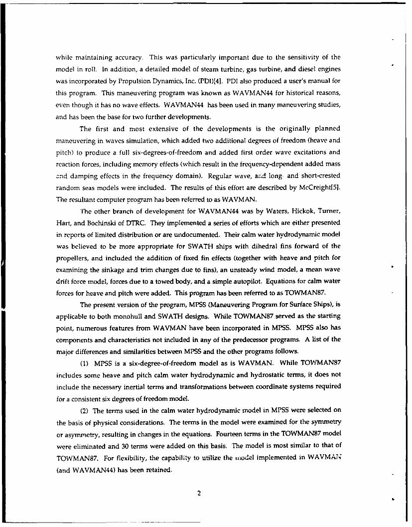
CALM WATER HYDRODYNAMIC FORCES

The calm water terms include the traditional maneuvering model and have evolved

over many years. The history and development of these terms was briefly outlined in the

introduction. The calm water forces and moments are represented as the sum of the product of

coefficients and state ariables. In the computer program, all terms are non-dimensionalized

using the SNAME system[8]. Following solution of the system of equations of motion, velocities

-n- dimensionalized. For simplicity, the equations presented here will be given in the

dimensional form. These forces are calculated in the maneuvering coordinate system.

The final expression for surge, sway, and heave forces and roll, pitch, and yaw momentsfollow.

XcV=Xl'u +XO+(X vv +X v F F) v2 + kX I+X rF F)r 2 +(X v + X , r vr vr

* ( XvO v + Xro rv + (Xdo + Xvvoo v2 + XrrO6 r2 + Xvroo v r ) 2

+ x -2 4 XFk8Fk

+ ( Xccee+ Xcce'W 02 ) c2e 2 + X.0e 0 + XRp

YcW (+Y+Y uu u 2 ) ,+ y w + Y p +Y + ( Ytr + Yhiuu +Y ruu u2 ) f

+(Yv+YvFF+YvF-F 2 )v+YpP+(Yr+YrFF+YrFFF 2 )r

+Yvlvl v lvl +Yvlrl v Irl +Yrrl r Irl +Yrlvl r lvI

+ (Yo + YOF F + YoplF F 2 )

+ (Yve v + Yv60 0)v 0) + Yvrb v r 0) + ( Yrro r + Yrb o) r io

+ (Y+Y88862+YFFF2)+Y8rl5 I + YFk Fk

+ ( Ycce + Ycce) e2 + y e42)cZ e

Zcw= Z ,+ w + , +7Z.rz+ Zu+Z vv+Zww+Zqq+Zrr

+ Zz 0 + Z 0 + Z8 F+ ZFkFk

7

KCW (K +K u u + K u u2 ), + Kv % + KO I) + K + Kri

+(KV+KvFF+Kv FF F2 )v+KP P +(Kr +KrFF+KrF F F2 )r

+Kvlvl v lvi +Kvlrl v Irl +Krlrl r Irl +Krivi r Ivi

+ (KO + K F F + KOFFF 2 )0

+(KwOV +KvOO O)vO+Kvr v r O+ ( K rr r + K r WO) r O

+(KS+K58s82+KBFFF2)8+ F KFkSFk

+ ( Kcce+ Kcceee e2 + Kcceo 02) c2 e

MCW= M(,*+w+Mp M +Mri Mu u+Mvv+Mww +Mqq+Mrr

+ M z0 M + M + 8 MFk8F k

NCW =(N, +N.,u u + NiwU2) - + N,.v * Np P + Nil t + ( Ni + Ni~u u + Ni.uu u2) i

+(N v +NvFF+NvFFF 2 )v+Npp +(Nr+NrFF+NrFFF 2 )r

+Nvvl v 1vi +Nvlrl v Irl +Nrlrl r Irl +Nrlvl r Ivi

+ ( No + NOF F + NOFF F2 ) 0

+ ( Nw¢ v + Nv,0 0 ) v + Nvro v r0 + ( Nrro r + Nro ) r 4

+(N6+N88882+N8FFF2)8+N81r SI1r +VjF NFk8Fk

+ ( Ncce+ Ncceee e2 + Ncceo 0 2 ) c2 e

In the above F is the Froude number, defined by U where U = 4 U2 + V2 + w2 is the

instantaneous forward speed of the ship and 8 is the rudder angle.NF is the number of fins installed, 8Fk is the angle of the kth fin. The fin model is

included to account for the effects of fins, particularly on SWATHs. As currently implemented,

the fin angle is assumed to be a constant which is set at the beginning of the run; that is, no

active control of fins is considered. The fins are assumed to be simple lifting surfaces mounted at

8

an arbitrary location and angle. The X force is proportional to the square of deflection, 6 Fi. It is

assumed that XF is minimum at 8F = 0.

The term XRp and the terms with coefficients with c and e for subscripts can be used to

represent the res.stance and propulsion model. Details of the resistance and propulsion model

are given in the following section.

The terms included in this hydrodynamic model were selected by considering the

physics of the flow around the hull, propellers, and rudders, and the likely functional

dependence of the resulting flow forces on the mean flow over the rudder, c, and the effective

angle of attack, e. Moderate order polynomials in these variables and absolute values of v and

r were considered. Terms were included in the model only if the resulting contribution would

have the expected symmetry or anti-symmetry. That is, surge force is symmetric; sway force,

yaw moment, and roll moment are asymmetric. Not all of the coefficients in the model are

required for all ships. In the current model, some asymmetry, as for single-screw ships, may be

excluded. In this case, appropriate terms may be added to the model.

Some terms included in several of the previous models mentioned in the introduction

would not satisfy this criterion. Some other terms are ones for which data is not likely to be

available. The appendix lists additional terms which have been utilized in previous models.

These terms have been retained in the computer program to provide flexibility.

The numerical values may be obtained either from model experiments or by prediction.

Smitt and Chislett[3], and reference 10 discuss model testing techniques. Acceleration terms

(Y , , etc.) may be predicted with reasonable accuracy by potential theory. For other

coefficients, predictions are usually not too reliable unless a similar hull is available.

Prediction techniques for the coefficients are beyond the scope of the report here. For example,

see reference 10 for information on the topic.

Resistance and Propulsion Model

The resistance and propulsion model calculates the net surge force XRp due to the calm

water resistance and the propellers. In this section, the current model for calculating XRp as

well as two older methods of calculating XRP will be presented. The older methods are

included for compatibility with older sets of coefficients.

The current method of calculating XRp has several advantages over these older

methods. First, flow due to the propellers is calculated and its effect on the rudder forces is

modelled explicitly, making possible greater accuracy over widely varying operating

conditions. Secondly, effects of speed on the non-dimensional coefficients should be eliminated,

except at high Froude numbers, and thus a single set of coefficients should suffice for all speeds.

In contrast, with the other models it is common to use separate sets of coefficients at different

9

speeds, which is necessary because in current practice the resistance and propulsion effects are

imbedded in coefficients which do not explicitly depend upon Froude number (for resistance)

and shaft speed (for thrust).

The net surge force due to calm water resistance and propulsion is given by:

XRP = N p Xcpro p (0 - t) T - RT

where Np is the number of propellers, t is the thrust deduction, T is the open water propeller

thrust per shaft, RT is the calm water resistance, and Xcprop is a coefficient which corrects for

possible inaccuracies in the calculated values of T, which is not necessarily well known.

Resistance is obtained by linear interpolation in a table of resistance coefficients which are

defined by:

CR =C= U2 L22

Propeller open water thrust and torque coefficients KT and KQ are represented in the form:

Kr T TcrT (15)- p n2 D4 = CKT0 + cKT1 JT + CK 2 JT2

pn2D 5 Q IJQ KQ2 jQ2 (16)

where JT is the advance coefficient UA / n D, n is the shaft speed, and D is the propeller

diameter. The speed of advance UA is given by U (1 - wt) where wt is the thrust wake fracticn.

JQ is defined similarly for torque using wq, the torque wake fraction. Given U, t, w, and a

machinery model as discussed in the following section, equations (15) and (16) can be solved for

n and T.

Finally, in this model two other quantities used in the force and moment model of the

previous section are also calculated. The mean flow over a rudder is given by:

c= A (1 - wt) u + k UAJ 2 + ( 1 -AR ) (1wt)2 u 2

where Ap is the area of the rudder directly behind the propeller and AR is the area of the

rudder, wt is the wake fraction of the propeller jet velocity at infinity and k = UA /UA. is afuntio of(xr-xp)whr

function of---f D here xr is the rudder location and- 3 the propeller location. k is derived

theoretically in reference 11. Reference 7 contains a convenient plot of this function. UA. is

10

given by:

w u +8KTUA = -(1 - wt) u + (1 -wt) 2 u 2 +-(nD) 2

Finally, the effective angle of attack of the flow over the rudder is given by:

e =-tan-1 v + rxrIc c 1

This is the version of propeller-rudder interaction model proposed by Abkowitz[71 following

Norrbin[6]. Use of c and e makes possible a more accurate calculation of the influence of

propeller speed on the forces and moments on the ship.

The first of the two older models is:

XRp=(1-t) NpT - RT

where T is defined by equation (15). RT for this model is given in pounds by:

RT=50 PER-U

where PE is the ship effective horsepower represented by a polynomial.

; PENp U3 - C-KP0 + CKPI U + CKp 2 U2 + CKp 3 U

3

The propeller thrust is calculated as in the first model.

The second of the two older models utilizes the simple expression:

XRp = Xu-ii + X- u2 + Xuu-u

where ii = u - UO is the speed loss and U0 is the initial forward speed of the ship. In this

model, hull resistance, propeller, and (implicitly) machinery dynamics are all combined into a

simple function of the speed loss.

Machinery Model

The machinery model governs the variation of propeller speed throughout the

maneuver. There exist three simple models and two detailed models. For the simple

machinery models, either speed, torque, or power is held constant. The detailed machinery

models are for either a diesel engine or a turbine and include the effects of engine dynamics,

11

governors, torque limiters, and drive train dynamics. The detailed models were developed by

Propulsion Dynamics, Inc.4] and will not be included here.

WIND FORCES

The wind forces and moments, FWIND, are b, ;d on data, CWIND, measured in a wind

tunnel for a range of headings. The wind force and moment coefficients, CWIND, are defined by

non-dimensionalizing the measured forces by -L L2U 2 and the moments by-L L3 U2 where PA is

the mass density of air.

This non-dimensional data, CWIND, are interpolated linearly in heading to obtain the

values for the correct relative wind direction, 4fW - , where WW is the wind heading:

o RW tan-, [ U W sin(aw - 40 - vi 1R= t [ cos6WW-) J (17)

where uI and vl are the ship velocities in the inertial coordinate system. FWIND is then

calculated by dimensionalizing the resultant values, CWIND(WRW). The force components are

dimensionalized by L L2 URW and the moment components by EA L3 where

URW =IUW cos(W - 4f) - u, 12 + I UW sin(Ww -W) - vI 2 (18)

The wind direction, W is measured relative to the x0 -axis, and is such that with the ship

parallel to the x0-axis, 14W = 00 is a following wind, iW = 90 ° is a port beam wind, and

w = 1800 is a head wind. In these equations, UW is the wind speed which will be defined in

the next section. These calculations are performed in the yawed coordinate system.

Unsteady Wind Model

An unsteady wind velocity model is incorporated using the Davenport[12] spectrum for

variation of the longitudinal component of the wind. No lateral spectrum is used at present, so

the direction of wind is assumed to be constant.

The unsteady wind velocity, Uw(t), used in equations (17) and (18) is given by:

Uw(t) = UWIND + SWIND (A + (19)

where UWIND is the mean wind velocity in knots at an elevation of 10 meters above the water

12

surface and the Davenport wind spectrum density function SWIND (Wj) in m2 / sec is given by:

1.459 x 105 K WoSWIND ((oj) = (1 + x2)4 / 3

(oj is the frequency in radians per second, j is the random phase, distributed uniformly over

(0,27], K is a drag coefficient taken as 0.005, and

x = 1.378 x 105U WIND

In the model, the spacing of the discrete oj is selected so that each component in the

summation of equation(19) has the same amplitude; the frequencies are spaced more closely

where the spectrum is larger.

Approximation for Wind Force Coefficients

If measured CWIND data are not available, an alternative is the model applied

previously by McCreight[5] for monohulls:

PAXWIND = T URW2 AF C x sin( I 'VR W I I I<

PAKWIN D = -T- URW2 AS Cy wma x sin(VRW)

SPA URW2 AS HS CK sin(ivRW) cos2 Wrnax

NWIND - 2 URW2 AF CNwma x sin( 2'RW

where AF, AS, HS, PA, p, and L are projected frontal and side above water areas, the vertical

coordinate of the centroid of the projected side area of the ship, air mass density, water mass

density, and ship length, respectively.

The values 0.70, 0.80, 1.30, 0.10 have been adopted for the wind force coefficientsCXwmax CYw max' CKwma x , and CNWmax' respectively. This approximation is based on

experimental results of Aage[131 for a number of ships. The roll dependence is adapted from

Sarchin and Goldberg[14].

13

WAVE FORCES

A seaway acting on a ship causes forces, some of which can be neglected in the

maneuvering problem and some which must be accounted for. The incident seas can be

represented using the model of St. Denis and Pierson[15], in which the sea surface C(x0 ,y0 ,t) is

represented as the sum of sine waves of varying lengths and dircctions.

C(x0 ,y0 ,t) = Re ; eiKk(X0 cospj+Y0 sinti ) + i(Okt + iFjk 5S( kgj Ajok

2ok

for short-crested seas, where Kk is the wave number - of the kth frequency 0Ok of mg

frequencies, pj is the jth of n directions, -jk is the random phase of the wave component of

frequency k and direction P, uniformly distributed over (0, 2] and S; is the Bretschneider[161

wave spectrum with cosine-squared spreading given by

S;(OkVj 2 cOs2 (g - g) S (Ok) 0 < I t - C I :5!

=0 i< I.-Pc < !57

and

-4-.24. o 2 - e 1944.5 T 0 4

2

where (C) 1/3 is the significant wave height, To is the modal, or peak energy, period and pc is

the (predominant) wave direction. The wave direction A is measured relative to the x0 axis,

and is such that with the ship parallel to the x0 -axis, p = 0* is a following wave, p = 900 is a

port beam wave, and p = 1800 is a head wave. This convention is the same as for the wind

heading.

For long-crested waves the appropriate expression is:

(x,y,t) = Re =1 e'iKk(XO cOs9+y0(t) singj) + iOakt + ick 2S (Wk) Ak

where p is the wave direction and Ek is the random phase uniformly distributed over (0,270.

Ogilvie[17] presents an excellent survey of the resulting forces and methods of

predicting them. Here we just give a brief summary of these forces and discuss the assumptions

14

and approximations used in the program for calculating the slowly-varying wave drift force

components, as well as indicate why the other terms were omitted.

For purposes of explanation, we now consider two plane waves of different lengths

propagating in the same direction

C(t) = A1 cos~olt +A2 cosw2 t

Assuming a perturbation expansion in the wave amplitudes A1 and A2 and ignoring terms

greater than quadratic, the forces are of the form:

F(t) = Re{A 1 Gl(co1) eiOlt+ A2 G1 (o 2) i2t) + 1 Re(A 1 G2 (c01,-(O1 ) + A 2 G2 (0o2 ,-(02 ) }

* 1 G2((01,(Ol) ei2olt) 1 R 2 e i2o)2t+ eA 2 co, 1 + R{2G2(co2,oa2) e

+ ReA 1 A2 G 2(o01,(o2) e i(O) 1 + (02 )t) + Re(Aj A2 G2(0 1 2 ) e i(0 - 0 2 )t) (20)

In equation (20) the first and second terms which are proportional to A1 and A2 , respectively,

are the linear exciting forces, which will be ignored in the present work. These are responsible

for the motions of ships in waves as predicted by the standard seakeeping programs, but the

motions are periodic, average out to zero, and thus are not of interest for the pure maneuvering

problem.

The remaining terms are the nonlinear wave forces. These are quite small in magnitude

relative to the first order forces, and are generally neglected in standard seakeeping studies.

Several of these are important for stationkeeping and trackkeeping studies, because while they

are small, their mean is non-zero and can cause considerable excursions in surge, sway, and yaw,2

where there are no restoring forces to balance them. The next two terms, proportional to A1 and

2A2 , respectively, are the mean drift forces, and are important. The next three terms,

i2colt i2wot i(031 + (02)tproportional to ei , ei , and e , respectively, act at even higher frequencies than

the incident waves, and thus are negligible. The last term, proportional to A1 A2 ei( 1

-

results in a slowly-varying drift force which is often also neglected, but may be important in

trackkeeping with strict requirements on the amount of drift permitted from the nominal

trackline. This is also impurtant for stationkeeping, but is traditionally ner,.e,.,d in the static

force balance approach often used in these problems. In the two wave case considered here, the

slowly-varying force is a simple sinusoidal beat at the difference frequency. The two main

expressions for forces of equation (20) can be extended to represent the responses to an irregular

15

seaway ii terms of single and double integrals (summations for the discrete case). Mcst of the

terms required in such an expression are unknown, however, and an approximate method must be

found, utilizing only the mean drift force operator G2((O,-(O).

Based on the discussion given above, only the slowly-varying drift forces will be

included in this model. That is,

FWAVE = FSVDF

where FSVDF will be defined in the next section utilizing the mean drift force operator

C,(o0,-)) which may be obtained from experimental data or from oredictions.

Slowly-Varying Wave Drift Force Model

In this program, slowly-varying wave drift forces in short-crested waves are calculated

by an approximate method due to Marthinsen [18]. This method is based on the assumption of a

narrow-banded spectrum and the idea of a local wave frequency and direction to enable the use

of regular wave drift force operators as the basis of the calculation. This is a more systematic

and general approach which is equivalent to the approximation of Hsu and Blenkern[19]. In

the case of a long-crested wave, Marthinsen showed through several examples that this

approach is equivalent to the commonly used approximate methods of Newman[20]. This

approximation uses only the regular wave drift force, which is the most readily available from

experiment or calculation. These forces are calculated in the yawed system.

We will not derive the method here. The calculation method is as follows:

Calculate the Hilbert transform of the wave elevation, which is given by

'n(xoy 0,t) =Im - - eiKk(XO cs+Y0 sint) ) + i(Okt + icjk S ((kvj) AiLj A0k

for the short-crested case and by

(x0,y0,t) = Im f -I eiKk(xO cosgj+Yo singj) + 1Okt + ick 2S((k)k

for the long-crested case. Then the instantaneous wave amplitude, frequency, wave number

components, and wave direction are given by:

A(t) = "C(t) 2 + T(t)2

CO = Tj8 _C(t) , / At)t)

kx(t) = n t) -V 7 / A2(t)

8x /8 Atkx_ 816

16

k(t) M= 8 - (t)(t A2(t)

ky~t)

W4(t) = tan "1 [ kv(t)

The resulting approximate expressions for the slowly-varying drift forces and moment are1

XSVDF = -2 P g L A2 (t) CX( ca(t), W(t) )

YSVDF =I p g L A2 (t) Cy( c(t), Wt(t) )1

NSVDF = p g L2 A2(t) CN( o(t), it(t))

where in the previous notation

Cx( CO(t), W(t) ) ( D1 pgL

represents the non-dimensional mean surge drift force for a regular wave of frequency (0 and

direction Vi and Cy and CN are similarly the non-dimensional drift force and moment for sway

and yaw, respectively.

In the simulation, the drift forces are updated only on', per second and are assumed

constant during the one second time interval. Further, in the initial phase of the simulation,

the forces are ramped up from 0 at t = 0 to the full value at t = teramp , which is an input

variable.

Strictly speaking, the slowly-varying drift force model is valid only for zero forward

speed, because experimental data is available only at zero speed. Utilizing the model at low

speeds is reasonable, however. At high speeds, drift forces are less significant because the hull

forces which are proportional to speed squared are dominant and can easily compensate for the

effect of drift forces.

TOW FORCES

The force, FTOW, due to towing a body through the water is also modelled. It is

assumed that the tow cable is parallel to the total ship velocity, U, and that the force is

proportional to the square of the total ship velocity. The tow point is located at (xT, YT, zT)"

KTOW = Ty zT

MTOW = Tx ZT

17

NTOW = Ty xT - Tx yT

where

Tx cos DTOw U2

U2'TOW

Tv sin P DTOW U2

U2

TOW

and DTOW is the drag at a reference speed of UTOW.

SOLUTION OF THE EQUATIONS OF MOTION

The program first initializes the state vectors for the ship and then the equations of

motion are integrated forward in time to obtain the specific solution for a given set of initial

conditions and rudder and speed commands. Turns, spirals, zig-zags, and arbitrary sequences of

rudder and speed changes may be commanded.

The initial conditions for the time domain solution are chosen to represent the steady

state solution corresponding to the ship moving at constant speed and heading, subject to the

wind and waves assumed. Mean values of unsteady wind and slowly-varying wave drift forces

are used during the initialization. The unsteady parts are ramped up from zero to full value at

a (user-specified) time after the beginning of the run. This is necessary in order to prevent

spurious starting transients in the solution.

The initial conditions are determined by minimizing the sum of the squares of the

accelerations in six degrees of freedom. This yields rudder angle, shaft horsepower, heave,

roll, pitch, and yaw (drift angle) to balance wind forces and forces due to asymmetry of the ship

calm water hydrodynamic model.

The method adopted for finding initial conditions yields solutions which result in

negligible starting transients. This has been demonstrated by running calm water solutions with

no steering or speed commands for periods of time up to 1000 seconds (full scale) which resulted

in essentially no change in the ship speed, heading, or attitude.

At any time t, the equations of motion, see equations (1-6), can be solved algebraically

for the acceleration in terms of the velocities, displacements, and forcing functions. Force and

moment components for hydrostatic, wind, wave drift, and tow forces are transformed to the

maneuvering coordinate system using equation (13) and then added to the calm water

hydrodynamic forces as in equation (14). Together with the kinematic relations of

18

equations (7-12) for the time derivatives of the position and orientation, and for certain

variables used in the (optional) machinery models, these form a system of differential

equations which are integrated numerically from the initial conditions as described in theprevious section to find the motion of the ship as a function of time. In the present program, an

adaptive Runge-Kutta method developed by Mersonl2l] is used.

Test runs in calm water conditions showed that predictions of sharp turns (rudder angle

35 degrees) were practically independent of step siz. for step sizes ranging from 0.0333 seconds

to 5.0 seconds. For step sizes greater than 1.0 seconds, the step reduction feature came into play

in the initial portion of the run when accelerations were largest.

CONCLUSION

This report describes a mathematical model to predict the motion of a surface ship

while maneuvering in calm water, including unsteady wind and slowly-varying wave drift

forces, and forces due to a towed body. This model incorporates a model of propeller-rudder

interaction based on the physics of the situation, rather than a simple curve fit to experimental

data as has been used previously. This mathematical model has been implemented in a

computer program, MPSS (Maneuvering Program for Surface Ships). Hydrodynamic coefficients

must be provided for the mathematical model. In addition, terms used in previous programs

which are not included in the model here may optionally be included. This program is

applicable to SWATH ships as well as monohulls.

19

This page is intentionally left blank.

20

APPENDIX - ADDITIONAL TERMS IN WAVMAN44 OR TOWMAN87

The purpose of this appendix is to present terms which are included in the calm water

forces and moments in WAVMAN44 or TOWMAN87, but are not included in the model

presented in this report. An option exists in MPSS so that these additional terms can be

utilized. This makes it possible to run MPSS using old data sets.

WAVMAN44 is a four-degrees-of-freedom program so that heave and pitch are not

included. In WAVMAN44, U is defined as Nu 2 + (w cos o)2, rather thanVu2 + v2 + w 2. This

U is used to dimensionalize the forces and moments. In addition, WAVMAN44 includes some of

the terms which are multiplied by F in the model presented in this report. However in

WAVMAN44 those terms are multiplied by t. u is defined as (u - U0 ) and U0 is the initial

forward speed of the ship. When the WAVMAN44 option is utilized in MPSS, the definition

of U stated here and the substitution of i for F will be implemented.WM WM WM WM

The additional terms in WAVMAN44, given as XCW , YCW, KC;V and NCW are:

WNMXCW =X.v +Xrtvl r IvI +XwFFv 2 F2

+ Xu85F U 2 F + X 8 5 + X88d 62 ii + X8du 8 i2

+ Xv8v5+Xr5r8+Xiiv 181 v+X5 lvi +Xvv8v2

YCW =Y+Yi v 2 Y +YvVrr +Yrrr '

+Yrvvrv2+Yr,vl rI1vl +Yoirl 0 Il +Yl0lr 101 r+yW0 3 +y880

+ Yvr8 v r 8 + YS5 8 v2 + Y8, 8 r2 + y88 2 + YvW v &2 + yr8 r 82 + YSvr 8 v r

+Y81vk 8 Ivi +Yv, 1 Vl 81+Y8ij5+Y 582 ?'u+Y86u583Ui

WMKCW = KldPUp+KIPI pipP +Kpip.jlp Ipl i+Knr 3 +Krv r 2 v

+ Kr r v2 + KvF v F + KvFF v F 2 + Kp/F p / F + KpF p F + KpFF p F 2

+Kioir 101 r+Klrl 0 Irl +Koo o3 +KZvlv 8 lvi +K 8i

WM

NCW = N0 + NO( + Nw v2 + NVVv v3 + Nvrr v r2

21

+Nrrrr3+Nrvvrv2+Nr'Niv -jvl +N0iri ) Irl +Nlblr 1)1 r+NOW 03

+N0 1 81 0 181 +Nvr5VrS+Nw6 v2 +Nrrr 2 +NS88 2

+NvS~V82+Nr88r82+NSvrSvr+NSivl 5 1v1 +NvlIlvI 81+NsdjiS

+ N&aS 82 U + N&S8i 83 U

While TOWMAN87 includes some heave and pitch calm water hydrodynamic and

hydrostatic terms, it does not include the necessary inertial terms and transformations between

coordinate systems required for a six degrees of freedom model.

TOWMAN87 includes calm water forces for heave and pitch. However, it does not

include the inertial terms and coordinate transformations required for a consistent six degrees of

freedom model. In TOWMAN87, U is defined as N]u 2 + (w cos 0)2, rather than u2 + v2 + w2 .

This U is used to dimensionalize the forces and moments. In addition, TOWMAN87 includes

the terms which are multiplied by F in the model presented in this report. However in

TOWMAN87 those terms are multiplied by powers of U. When the TOWMAN87 option is

utilized in MPSS, the definition of U stated here and the substitution of U for F will be

implemented when the flag indicating TOWMAN87 data is set in the input. The additionalTM TM TM TMterms in TOWMAN87, given as XCW YCW, MCW, and NCW are:

TMXCW = X8 8 + XSU 8 U

TMYCW = Yvvv v 3 + YvO v 0+ Yro r 0 + Yv 8 v

TMKCW= Kvv)+K, ,o ro

TMMCW = MO 4

TMNCW = Nrv T V + Nvvv v3 + Nvv v 0+Nav8v

22

REFERENCES

1. Strom-Tejsen, J. "A Digital Computer Technique for the Prediction of Standard Maneuversof Surface Ships," DTMB Report 2130, December 1965.

2. Abkowitz, Martin A., "Lectures on Ship Hydrodynamics, Steering and Maneuverability,"Hydro-og Aerodynamisk Laboratorium Report No. Hy-5, Lyngby, Denmark, May 1964.

3. Smitt, L. W. and M. S. Chislett, "Large Amplitude PMM Tests and Maneuvering Predictionsfor a Mariner Class Vessel," Tenth ONR Symposium on Naval Hydrodynamics, Boston, Jun1974.

4. Propulsion Dynamics, Inc., "Implementation of Turbine and Diesel Propulsion SystemMoels in a Surface Ship Maneuvering Simulation," DTNSRDC Report SPD-CR-003-82, Mar1982.

5. McCreight, W. R., "Ship Maneuvering in Waves," Sixteenth Symposium on NavalHydrodynamics, Berkeley, 1986.

6. Norrbin, Nils H., "Theory and Observation on the use of a Mathematical Model for ShipManeuvering in Deep and Confined Waters," Publications of the Swedish State Ship BuildingExperimental Tank, No. 68, Goteborg, 1971.

7. Abkowitz, M. A., "Measurement of Hydrodynamic Characteristics from Ship Trials bySystem Identification, Transactions of the Society of Naval Architects and Marine Engineers,Vol. 88, 1980.

8. ----. , "Nomenclature for Treating the Motion of a Submerged Body through a Fluid,"Society of Naval Architects and Marine Engineers, Technical and Research Bulletin 1-5, NewYork, 1950.

9. Salvesen, N., E. 0. Tuck, and 0. M. Faltinsen, "Ship Motions and Sea Loads," Transactionsof the Society of Naval Architects and Marine Engineers, Vol. 78, 1970.

10. Crane, C. Lincoln, Haruzo Eda, and Alexander C. Landsburg, "Controllability," Chapter 9of Principles of Naval Architecture. Volume III E.V. Lewis, editor, The Society of NavalArchitects and Marine Engineers, New York, 1989.

11. Gutsche, F. "Die Induktion der axialen Strahlzusatsgeschwindigkeit in der Umgebung derSchraubenebene, Schiffstechnik, Bd 3, 1955.

12. Davenport, A. G., "The Spectrum of Horizontal Gustiness Near the Ground in High Winds,"Quarterly Journal of the Royal Meteorological Society, Vol. 84, pp. 194-211, April 1961.

13. Aage, C., "Wind Coefficients for Nine Ship Models," Hydro-og AerodynamiskLaboratorium Report No. A-3, May 1971.

14. Sarchin, T. H. and L. L. Goldberg, "Stability and Buoyancy Criteria for U.S. Naval SurfaceShips," Transactions of the Society of Naval Architects and Marine Engineers, Vol. 70, 1962.

15. St. Denis, M. and W. J. Pierson, Jr., "On the Motion of Ships in Confused Seas," Transactionsof the Society of Naval architects and Marine Engineers, Vol. 61, 1953.

23

16. Bretschneider, C. L., "Wave Variability and Wave Spectra for Wind-Generated GravityWaves," Technical Memorandum 118, U.S. Army Beach Erosion Board, Washington, D.C, 1959.

17. Ogilvie, T. F., "Second-order Hydrodynamic Effects on Ocean Platforms, InternationalWorkshop on Ship and Platform Motions, University of California, Berkeley, 1983.

18. Marthinsen, T., "Calculation of Slowly-Varying Drift Forces, Applied Ocean ResearchVol. 5 No. 3., pp. 141-144, 1983.

19. Hsu and Blenkern, "Analysis of Peak Mooring Forces Caused by Slow Vessel DriftOscillations in Random Seas,' Paper 1159 Offshore Technology Conference, Houston, 1970.

20. Newman, J. N., "Second-Order, Slowly Varying Forces on Vessels in Irregular Waves,"International Symposium on Marinp Vehicles and Structures in Waves, Institution ofMechanical Engineers, London, 1974.

21. Fox, L., "Numerical Solution of Ordinary and Partial Differential Equations," Addison-Wesley, Reading, Massachusetts, 1962.

24