Embed Size (px)
Citation preview
DTU IMM
MSc Thesis
Analysis and Optimization of TTEthernet-based Safety Critical EmbeddedSystems
Radoslav Hristov Todorovs080990
16-08-2010

Acknowledgements
The work for this master thesis project continued 6 months. This was a time when I
encountered a lot of problems and challenges. For the resolution of and the help provided
for many of them, I am glad to say “Thank you” to whom were involved.
On first place, I would like to thank my supervisor, Paul Pop. He invited me to start
this project and also helped a lot with the establishment of the problem. Furthermore, our
meetings were always beneficial and extremely encouraging in the period when I still did not
have complete understanding of the domain of my thesis. Thanks to him, I was introduced
to similar problematic that was very helpful for the solving of my assignment. Thank you
for the support!
Next, I thank my family that was very understandable and supportive during the last
half an year.
I would like to say great “Thank you” to Roxana. She was the one I could rely on
everything in my daily life.
I am thankful to my colleges from my workplace. They were very patient with me not
only during this project but also during my entire education in DTU.
Special thanks to Philip for the correction of my English writing.
August 2010, Lyngby
1
Contents
1 Background 1
1.1 Introduction . . . . . . . . . . . . . . . . . . . . . . . . . . . . . . . . . . . . . 1
1.2 Avionic networks and IMA . . . . . . . . . . . . . . . . . . . . . . . . . . . . 2
1.3 TTEthernet . . . . . . . . . . . . . . . . . . . . . . . . . . . . . . . . . . . . . 7
1.4 AFDX . . . . . . . . . . . . . . . . . . . . . . . . . . . . . . . . . . . . . . . . 14
1.5 Integration . . . . . . . . . . . . . . . . . . . . . . . . . . . . . . . . . . . . . 25
2 Motivation 26
2.1 Introduction . . . . . . . . . . . . . . . . . . . . . . . . . . . . . . . . . . . . . 26
2.2 Hardware Architecture . . . . . . . . . . . . . . . . . . . . . . . . . . . . . . . 27
2.3 Software Architecture . . . . . . . . . . . . . . . . . . . . . . . . . . . . . . . 29
2.4 Application model . . . . . . . . . . . . . . . . . . . . . . . . . . . . . . . . . 31
2.5 Technological notations . . . . . . . . . . . . . . . . . . . . . . . . . . . . . . 33
2.6 Problem formulation . . . . . . . . . . . . . . . . . . . . . . . . . . . . . . . . 34
3 End-to-end delay analysis 37
3.1 Introduction . . . . . . . . . . . . . . . . . . . . . . . . . . . . . . . . . . . . . 37
3.2 State Of The Art . . . . . . . . . . . . . . . . . . . . . . . . . . . . . . . . . . 38
3.3 Assumptions . . . . . . . . . . . . . . . . . . . . . . . . . . . . . . . . . . . . 46
3.4 Preliminary Analysis . . . . . . . . . . . . . . . . . . . . . . . . . . . . . . . . 47
3.5 Trajectory Approach . . . . . . . . . . . . . . . . . . . . . . . . . . . . . . . . 54
2
CONTENTS CONTENTS
3.6 Computations . . . . . . . . . . . . . . . . . . . . . . . . . . . . . . . . . . . . 60
4 (II) and (TT) messages 68
4.1 Introduction . . . . . . . . . . . . . . . . . . . . . . . . . . . . . . . . . . . . . 68
4.2 Indirect Influence (II) . . . . . . . . . . . . . . . . . . . . . . . . . . . . . . . 69
4.3 Time-Triggered (TT) messages . . . . . . . . . . . . . . . . . . . . . . . . . . 73
5 Evaluation 78
5.1 Introduction . . . . . . . . . . . . . . . . . . . . . . . . . . . . . . . . . . . . . 78
5.2 Case Study 2 . . . . . . . . . . . . . . . . . . . . . . . . . . . . . . . . . . . . 79
5.3 Comparison . . . . . . . . . . . . . . . . . . . . . . . . . . . . . . . . . . . . . 89
6 Implementation 92
6.1 Introduction . . . . . . . . . . . . . . . . . . . . . . . . . . . . . . . . . . . . . 92
6.2 Input model . . . . . . . . . . . . . . . . . . . . . . . . . . . . . . . . . . . . . 93
6.3 Preliminary setup . . . . . . . . . . . . . . . . . . . . . . . . . . . . . . . . . . 94
6.4 Calculation algorithm . . . . . . . . . . . . . . . . . . . . . . . . . . . . . . . 95
7 Conclusion 97
A Input and Output files 103
3
List of Figures
1.1 IMA architecture . . . . . . . . . . . . . . . . . . . . . . . . . . . . . . . . . . 3
1.2 IMA cabinets . . . . . . . . . . . . . . . . . . . . . . . . . . . . . . . . . . . . 3
1.3 Open IMA architecture - detailed view . . . . . . . . . . . . . . . . . . . . . . 4
1.4 Open IMA network architecture . . . . . . . . . . . . . . . . . . . . . . . . . . 5
1.5 Safety-critical TTEthernet network . . . . . . . . . . . . . . . . . . . . . . . . 7
1.6 TTEthernet — Traffic Integration . . . . . . . . . . . . . . . . . . . . . . . . 9
1.7 TTEthernet — protocol integration with Ethernet . . . . . . . . . . . . . . . 10
1.8 TTEthernet — Synchronization approach . . . . . . . . . . . . . . . . . . . . 13
1.9 TTEthernet — Synchronization levels . . . . . . . . . . . . . . . . . . . . . . 13
1.10 AFDX network . . . . . . . . . . . . . . . . . . . . . . . . . . . . . . . . . . . 15
1.11 End Systems and Avionics Subsystems . . . . . . . . . . . . . . . . . . . . . . 16
1.12 End Systems — Architecture and principle of communication . . . . . . . . . 17
1.13 Virtual Link . . . . . . . . . . . . . . . . . . . . . . . . . . . . . . . . . . . . . 18
1.14 Virtual Link — Traffic Regulator . . . . . . . . . . . . . . . . . . . . . . . . . 19
1.15 Virtual Link . . . . . . . . . . . . . . . . . . . . . . . . . . . . . . . . . . . . . 20
1.16 AFDX Latency in communication . . . . . . . . . . . . . . . . . . . . . . . . . 21
1.17 AFDX Switch . . . . . . . . . . . . . . . . . . . . . . . . . . . . . . . . . . . . 22
2.1 Illustrative AFDX configuration . . . . . . . . . . . . . . . . . . . . . . . . . . 27
2.2 Relation between hardware configuration and application model . . . . . . . . 31
4
LIST OF FIGURES LIST OF FIGURES
3.1 Examinating the dependecy from other virtual links . . . . . . . . . . . . . . 49
3.2 Examinating dependency on other Indirect Influence virtual links . . . . . . . 50
3.3 Virtual link V1 has the first message from all virtual links ready for transmission 51
3.4 Virtual link Vx is indirectly influenced by virtual links - II1 and II2 . . . . . 52
3.5 Virtual link V2 has the first message from all virtual links ready for transmission 52
3.6 Virtual link V3 has the first message from all virtual links ready for transmission 53
3.7 Configuration example on which the Trajectory approach is tested . . . . . . 54
3.8 Configuration example on which the Trajectory approach is tested — time
line diagram for virtual link V1 . . . . . . . . . . . . . . . . . . . . . . . . . . 56
3.9 End-to-end delay of a packet m . . . . . . . . . . . . . . . . . . . . . . . . . . 56
3.10 End-to-end delay of a packet VL1 — formula starting times . . . . . . . . . . 58
4.1 Example of extended configuration developed from the architecture depicted
in Figure B.6 . . . . . . . . . . . . . . . . . . . . . . . . . . . . . . . . . . . . 69
4.2 Example configuration with Time-Triggered (TT) messages on which the Tra-
jectory approach is tested . . . . . . . . . . . . . . . . . . . . . . . . . . . . . 74
4.3 Example configuration on which the Trajectory approach is tested . . . . . . 74
4.4 BAG of Time-Triggered (TT) messages . . . . . . . . . . . . . . . . . . . . . 77
5.1 Configuration example on which the Trajectory approach is tested . . . . . . 79
5.2 Total worst-case response times for Holistic and Trajectory approaches in
Case Study 1 . . . . . . . . . . . . . . . . . . . . . . . . . . . . . . . . . . . . 90
5.3 Improvement (in %) achieved by the Trajectory approach compared to the
Holistic approach in Case Study 1 . . . . . . . . . . . . . . . . . . . . . . . . 90
5.4 Total worst-case response time for Holistic and Trajectory approaches in Case
Study 2 . . . . . . . . . . . . . . . . . . . . . . . . . . . . . . . . . . . . . . . 91
5.5 Improvement (in %) achieved by the Trajectory approach compared to the
Holistic approach in Case Study 2 . . . . . . . . . . . . . . . . . . . . . . . . 91
A.1 Test 1 configuration . . . . . . . . . . . . . . . . . . . . . . . . . . . . . . . . 103
5
LIST OF FIGURES LIST OF FIGURES
A.2 Test 2 configuration . . . . . . . . . . . . . . . . . . . . . . . . . . . . . . . . 105
A.3 Test 3 configuration . . . . . . . . . . . . . . . . . . . . . . . . . . . . . . . . 109
A.4 Test 4 configuration . . . . . . . . . . . . . . . . . . . . . . . . . . . . . . . . 112
A.5 Test 5 configuration . . . . . . . . . . . . . . . . . . . . . . . . . . . . . . . . 116
A.6 Test 6 configuration . . . . . . . . . . . . . . . . . . . . . . . . . . . . . . . . 118
A.7 Test 6 configuration (with Time-Triggered messages) . . . . . . . . . . . . . . 118
6
List of Tables
1.1 Virtual Link — permissible BAG values and respective frequency of the link . 18
3.1 Comparison between all known methods for measuring of end-to-end delays . 45
3.2 Virtual link data for the example depicted on 3.7 . . . . . . . . . . . . . . . . 55
4.1 Virtual link V4 parameters . . . . . . . . . . . . . . . . . . . . . . . . . . . . . 70
5.1 Virtual link data for the example depicted on 5.1 . . . . . . . . . . . . . . . . 80
5.2 Case Study 1 — Holistic vs. Trajectory Approach . . . . . . . . . . . . . . . 89
5.3 Case Study 2 — Holistic vs. Trajectory Approach . . . . . . . . . . . . . . . 90
7
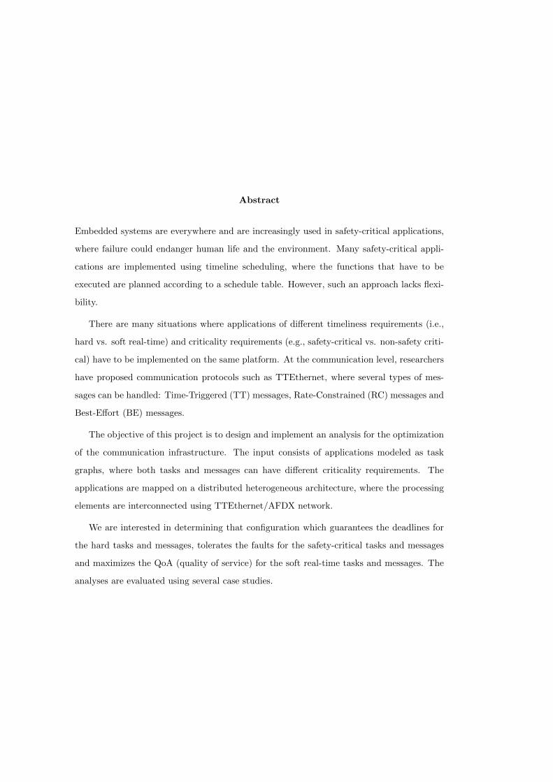
Abstract
Embedded systems are everywhere and are increasingly used in safety-critical applications,
where failure could endanger human life and the environment. Many safety-critical appli-
cations are implemented using timeline scheduling, where the functions that have to be
executed are planned according to a schedule table. However, such an approach lacks flexi-
bility.
There are many situations where applications of different timeliness requirements (i.e.,
hard vs. soft real-time) and criticality requirements (e.g., safety-critical vs. non-safety criti-
cal) have to be implemented on the same platform. At the communication level, researchers
have proposed communication protocols such as TTEthernet, where several types of mes-
sages can be handled: Time-Triggered (TT) messages, Rate-Constrained (RC) messages and
Best-Effort (BE) messages.
The objective of this project is to design and implement an analysis for the optimization
of the communication infrastructure. The input consists of applications modeled as task
graphs, where both tasks and messages can have different criticality requirements. The
applications are mapped on a distributed heterogeneous architecture, where the processing
elements are interconnected using TTEthernet/AFDX network.
We are interested in determining that configuration which guarantees the deadlines for
the hard tasks and messages, tolerates the faults for the safety-critical tasks and messages
and maximizes the QoA (quality of service) for the soft real-time tasks and messages. The
analyses are evaluated using several case studies.
Chapter 1
Background
1.1 Introduction
The main purpose of this chapter is to provide the necessary background for the further
work presented in this thesis project.
First, we give a short history of and introduction to the current state of the art of avionics
networks, the de facto Integrated Modular Avionics (IMA).
Afterwards, we discuss two current standards:
� TTEthernet (Time-Triggered Ethernet) as a novel integrating infrastructure for trans-
parent and fault-tolerant clock synchronization protocol
� AFDX (Avionics Full-Duplex Switched Ethernet), ARINC 664 Part 7, as a standard
that defines the specifications for exchange of data between Avionics Subsystems1 by
means of asynchronous messaging.
Finally, the chapter concludes with directions in how these two technologies are used in
terms of the architecture explored in this project.
1End nodes in an avionics network
1
1.2. AVIONIC NETWORKS AND IMA CHAPTER 1. BACKGROUND
1.2 Avionic networks and IMA
1.2.1 Classical approaches
The term “avionic” stands for “aviation electronic” components. Devices like these are
used for different types of electronic equipment applied to an aircraft. The present-day
avionics industry embraces a wide variety of components with ever more and more complex
functionalities. Thus, the development and the integration of a new avionics communication
network was required to address the amount of exchanged data and the communications
between the different network nodes. The classical concept “one function = one computer”
could be no longer maintained. This led to “federated architectures”, which integrates
several software functions in one hardware component. However, multifunction integration
prone to non-transparent fault propagation, and the maintenance of avionics systems of this
type becomes nightmare [1].
1.2.2 Integrated Modular Avionics — IMA
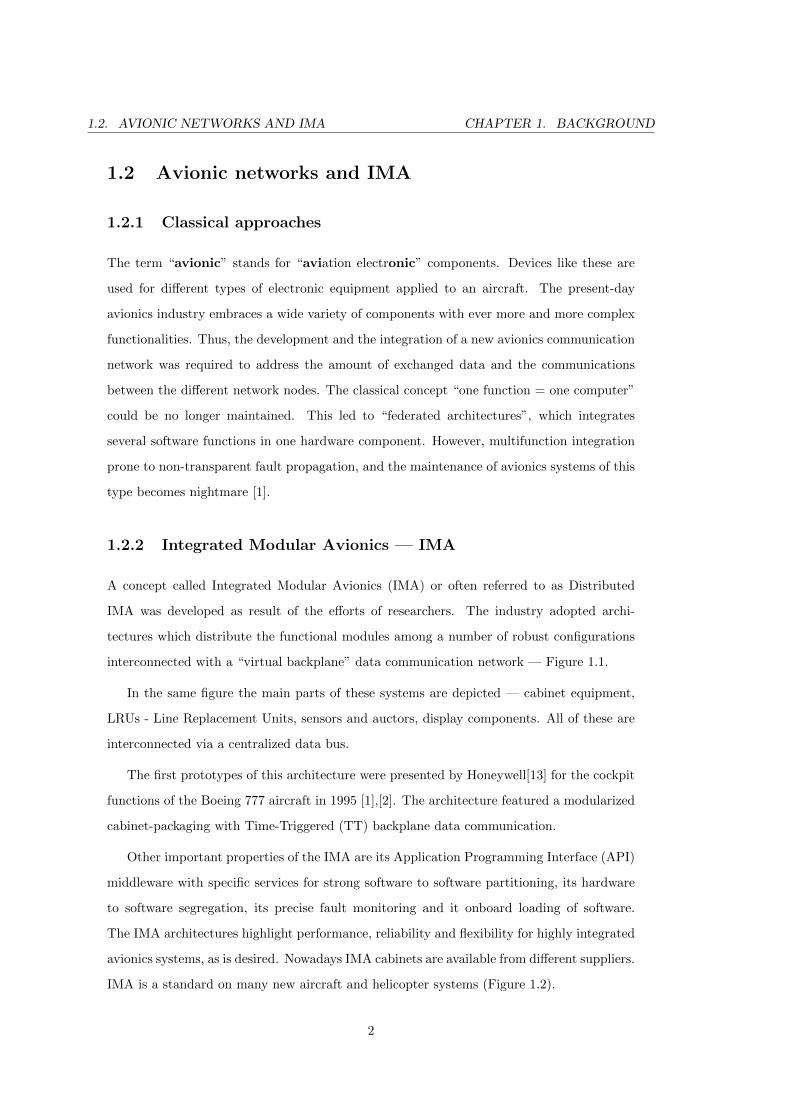
A concept called Integrated Modular Avionics (IMA) or often referred to as Distributed
IMA was developed as result of the efforts of researchers. The industry adopted archi-
tectures which distribute the functional modules among a number of robust configurations
interconnected with a “virtual backplane” data communication network — Figure 1.1.
In the same figure the main parts of these systems are depicted — cabinet equipment,
LRUs - Line Replacement Units, sensors and auctors, display components. All of these are
interconnected via a centralized data bus.
The first prototypes of this architecture were presented by Honeywell[13] for the cockpit
functions of the Boeing 777 aircraft in 1995 [1],[2]. The architecture featured a modularized
cabinet-packaging with Time-Triggered (TT) backplane data communication.
Other important properties of the IMA are its Application Programming Interface (API)
middleware with specific services for strong software to software partitioning, its hardware
to software segregation, its precise fault monitoring and it onboard loading of software.
The IMA architectures highlight performance, reliability and flexibility for highly integrated
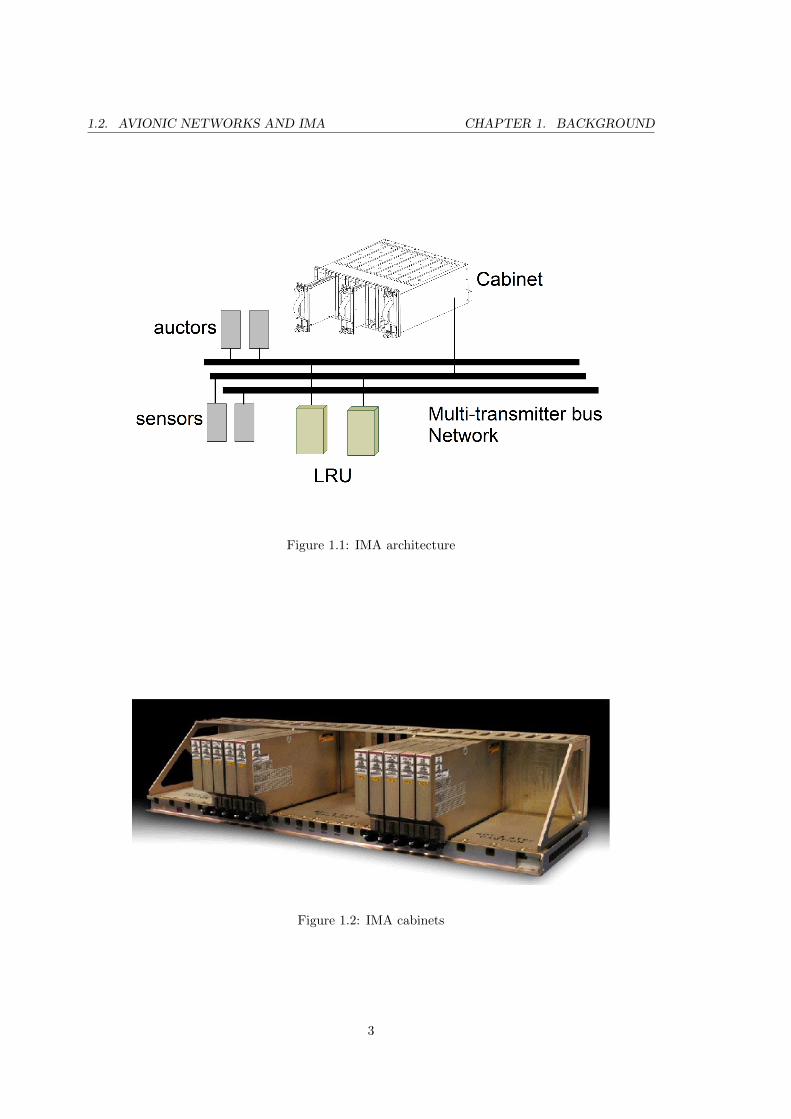
avionics systems, as is desired. Nowadays IMA cabinets are available from different suppliers.
IMA is a standard on many new aircraft and helicopter systems (Figure 1.2).
2
1.2. AVIONIC NETWORKS AND IMA CHAPTER 1. BACKGROUND
Figure 1.1: IMA architecture
Figure 1.2: IMA cabinets
3
1.2. AVIONIC NETWORKS AND IMA CHAPTER 1. BACKGROUND
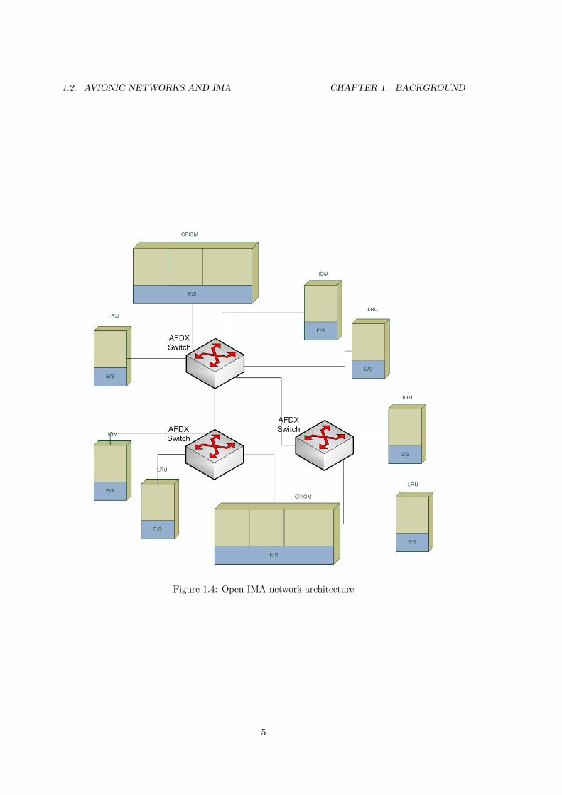
1.2.3 Open IMA and Aircraft Full DupleX (AFDX)
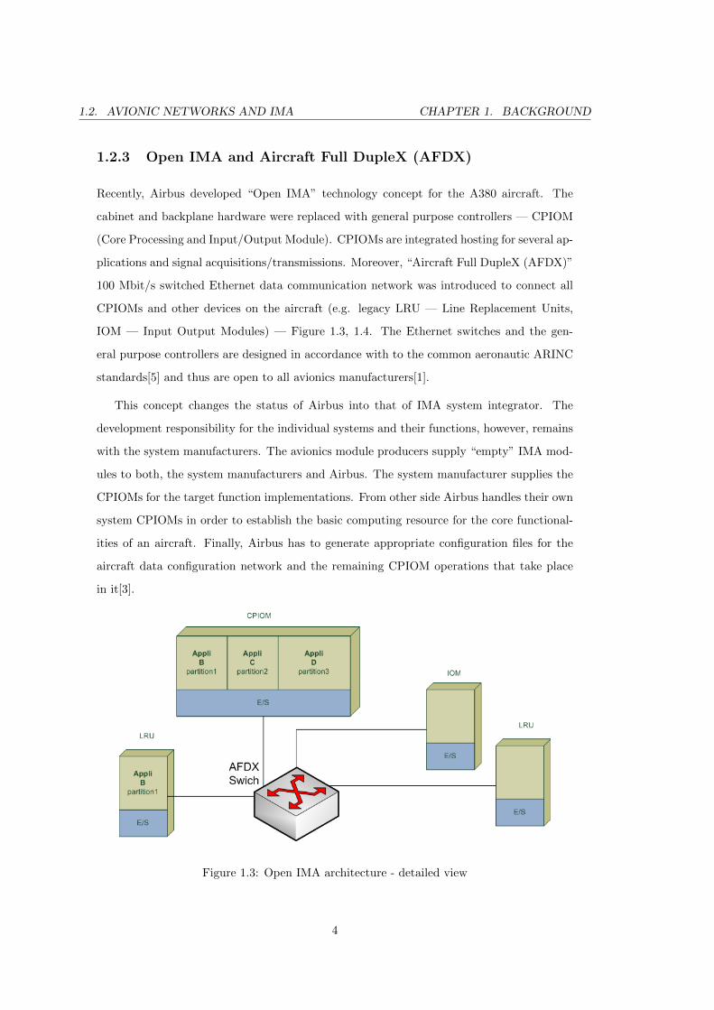
Recently, Airbus developed “Open IMA” technology concept for the A380 aircraft. The
cabinet and backplane hardware were replaced with general purpose controllers — CPIOM
(Core Processing and Input/Output Module). CPIOMs are integrated hosting for several ap-
plications and signal acquisitions/transmissions. Moreover, “Aircraft Full DupleX (AFDX)”
100 Mbit/s switched Ethernet data communication network was introduced to connect all
CPIOMs and other devices on the aircraft (e.g. legacy LRU — Line Replacement Units,
IOM — Input Output Modules) — Figure 1.3, 1.4. The Ethernet switches and the gen-
eral purpose controllers are designed in accordance with to the common aeronautic ARINC
standards[5] and thus are open to all avionics manufacturers[1].
This concept changes the status of Airbus into that of IMA system integrator. The
development responsibility for the individual systems and their functions, however, remains
with the system manufacturers. The avionics module producers supply “empty” IMA mod-
ules to both, the system manufacturers and Airbus. The system manufacturer supplies the
CPIOMs for the target function implementations. From other side Airbus handles their own
system CPIOMs in order to establish the basic computing resource for the core functional-
ities of an aircraft. Finally, Airbus has to generate appropriate configuration files for the
aircraft data configuration network and the remaining CPIOM operations that take place
in it[3].
Figure 1.3: Open IMA architecture - detailed view
4
1.2. AVIONIC NETWORKS AND IMA CHAPTER 1. BACKGROUND
Figure 1.4: Open IMA network architecture
5
1.2. AVIONIC NETWORKS AND IMA CHAPTER 1. BACKGROUND
The configuration part mainly concerns the switches, and more specifically the Ethernet
address tables, the prescribed transmission rate and the required bandwidth of a commu-
nication channel (virtual link). Adding new modules or changing existing subscribers to
the network needs only the establishment of a new virtual link between the transmitting
and the receiving device. This makes the configuration and the modification of the avionics
architecture flexible and scalable.
1.2.4 Recap
There are several standards produced and maintained by ARINC[5] covering the onboard
data communication in an aircraft. It was in relation to this that we presented in this section
the IMA concept. In conclusion, the new AIRBUS IMA concept contributes the following
features:
� modularized packaging connected to an AFDX network
� robust partitioning of the computing resources and communications
� determinism of the application execution and data exchanges
� standard APIs
� scope for interfacing with conventional equipment
6
1.3. TTETHERNET CHAPTER 1. BACKGROUND
1.3 TTEthernet
Among the major problems related to the design of an avionics network are the synchro-
nization strategies and predictability of the operations (determinism) while the network is
in operational mode.
The TTEthernet technology, developed by TTTech Computertechnik AG[12], inspired
by the academic TT-Ethernet[14] and covered by specification SAE AS6802 (of the same
organization)[11], offers synchronization operations based on integrated time-triggered and
event-triggered traffic.
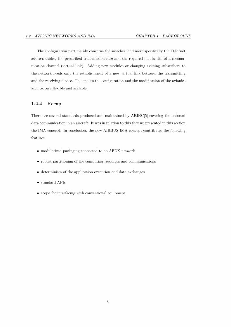
Figure 1.5 shows network of the denoted type, including a fault-tolerant configuration
capability. The network consists of host end systems with time-triggered Ethernet controllers
and two replicated store-and-forward switches interconnected with bidirectional point-to-
point links. The switches have a guardian function related to the fault-tolerant capabilities
of the network[14].
Figure 1.5: Safety-critical TTEthernet network
7
1.3. TTETHERNET CHAPTER 1. BACKGROUND
TTEthernet uses only standard Ethernet-compliant frames and thus remains compatible
with the underlying Ethernet. In fact, any technology could be chosen for an integrated
communication infrastructure, but Ethernet has also significant benefits. Ethernet is the
dominating standard for business communication, and, furthermore, there is a trend towards
applying it for distributed control systems. Areas where Ethernet has already been used for
solutions are industrial applications, the automotive industry and the avionics industry.
1.3.1 Traffic Classes[17], [16], [15]
The technology provides three traffic classes: Time-Triggered (TT) traffic, Rate-Constrained
(RC) traffic (this traffic is compliant with the AFDX traffic) and Best-Effort (BE) traffic.
Time-Triggered (TT) frames are used for applications with tight latency, jitter and de-
terminism requirements. All Time-Triggered (TT) messages are sent at predefined time slots
and they take precedence over the rest of the traffic. Time-Triggered (TT) traffic is opti-
mized for communication in distributed real-time systems with hard deadlines. Examples of
usage could be brake-by-wire and steer-by-wire systems, which use intensively rapid control
checking over the network and where the response time of the data is crucial.
Rate-Constrained (RC) messages are used for applications with less determinism and
real-time requirements. Rate-Constrained (RC) messages guarantee that their bandwidth is
predefined for each sender and the delays are within limited and predetermined boundaries.
Different controllers can send Rate-Constrained (RC) messages at the same time to the
same receiver or multiple receivers. In this case the messages may as a consequence queue
up in the network switches, which therefore need to have enough capacity. Otherwise there
will be an increase in the messages’ jitters and response times. The a priori setting of the
bandwidth and the intensity (period) of these messages is important realization for their
assets. From here their jitter and worst-case response time could be calculated offline .
The Best-Effort traffic (BE) is comparable with present-day Internet communication.
This means there is no guarantee whether the message is sent or when it will be sent. There
is no guarantee how long delay the message will incur before it arrives to its destination.
Best-Effort (BE) messages do not take precedence over any of the other traffic classes and
do not provide QoS (Quality Of Service) guarantees.
8
1.3. TTETHERNET CHAPTER 1. BACKGROUND
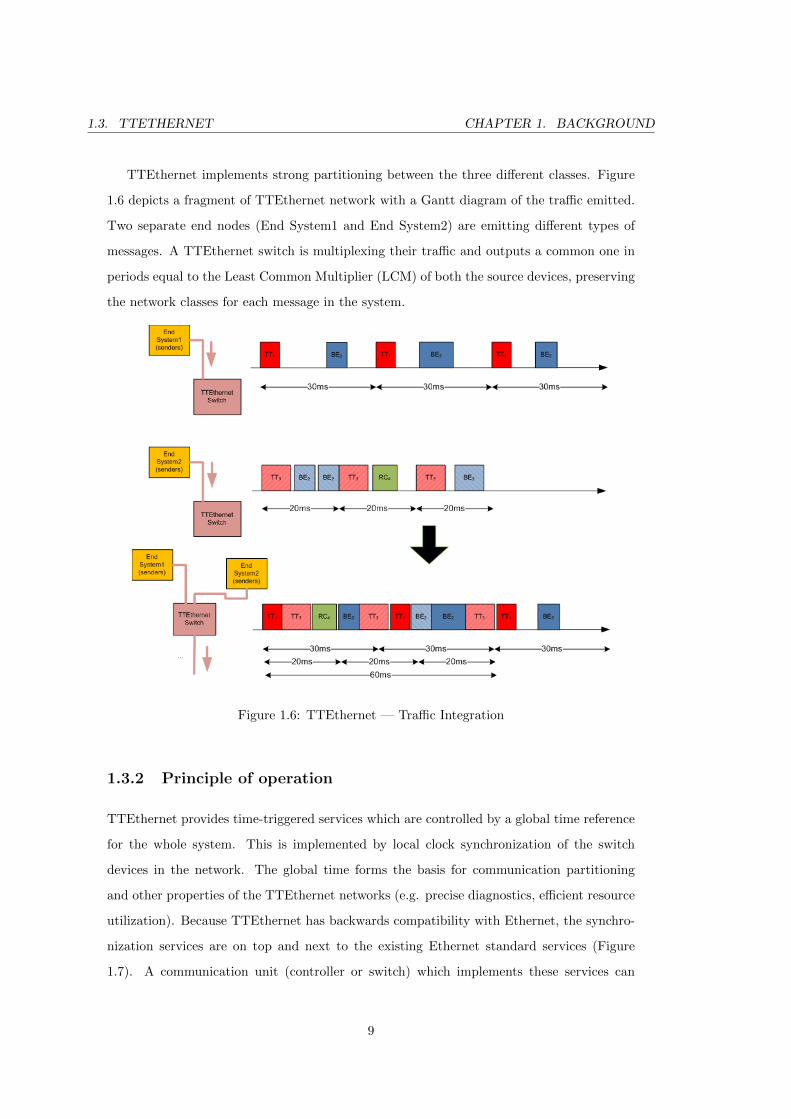
TTEthernet implements strong partitioning between the three different classes. Figure
1.6 depicts a fragment of TTEthernet network with a Gantt diagram of the traffic emitted.
Two separate end nodes (End System1 and End System2) are emitting different types of
messages. A TTEthernet switch is multiplexing their traffic and outputs a common one in
periods equal to the Least Common Multiplier (LCM) of both the source devices, preserving
the network classes for each message in the system.
Figure 1.6: TTEthernet — Traffic Integration
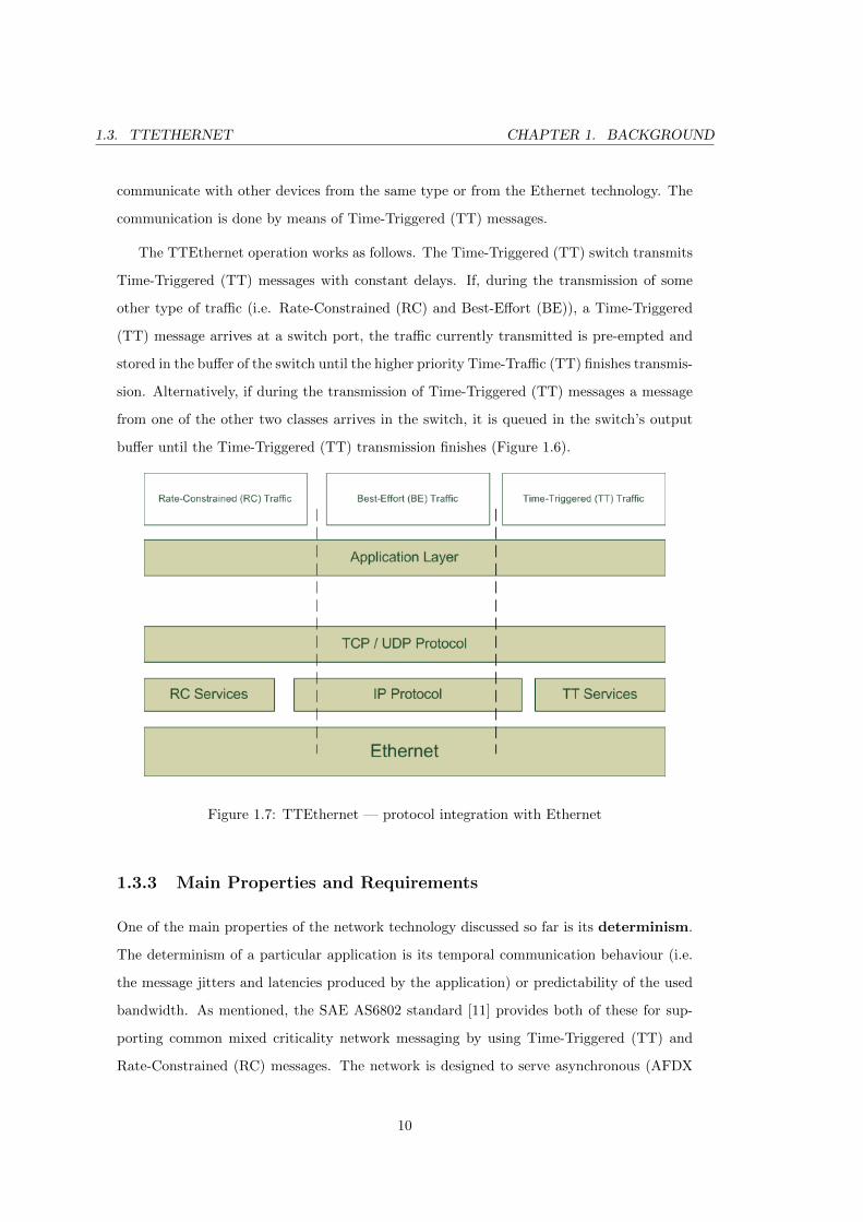
1.3.2 Principle of operation
TTEthernet provides time-triggered services which are controlled by a global time reference
for the whole system. This is implemented by local clock synchronization of the switch
devices in the network. The global time forms the basis for communication partitioning
and other properties of the TTEthernet networks (e.g. precise diagnostics, efficient resource
utilization). Because TTEthernet has backwards compatibility with Ethernet, the synchro-
nization services are on top and next to the existing Ethernet standard services (Figure
1.7). A communication unit (controller or switch) which implements these services can
9
1.3. TTETHERNET CHAPTER 1. BACKGROUND
communicate with other devices from the same type or from the Ethernet technology. The
communication is done by means of Time-Triggered (TT) messages.
The TTEthernet operation works as follows. The Time-Triggered (TT) switch transmits
Time-Triggered (TT) messages with constant delays. If, during the transmission of some
other type of traffic (i.e. Rate-Constrained (RC) and Best-Effort (BE)), a Time-Triggered
(TT) message arrives at a switch port, the traffic currently transmitted is pre-empted and
stored in the buffer of the switch until the higher priority Time-Traffic (TT) finishes transmis-
sion. Alternatively, if during the transmission of Time-Triggered (TT) messages a message
from one of the other two classes arrives in the switch, it is queued in the switch’s output
buffer until the Time-Triggered (TT) transmission finishes (Figure 1.6).
Figure 1.7: TTEthernet — protocol integration with Ethernet
1.3.3 Main Properties and Requirements
One of the main properties of the network technology discussed so far is its determinism.
The determinism of a particular application is its temporal communication behaviour (i.e.
the message jitters and latencies produced by the application) or predictability of the used
bandwidth. As mentioned, the SAE AS6802 standard [11] provides both of these for sup-
porting common mixed criticality network messaging by using Time-Triggered (TT) and
Rate-Constrained (RC) messages. The network is designed to serve asynchronous (AFDX
10
1.3. TTETHERNET CHAPTER 1. BACKGROUND
— Rate-Constrained (RC) messages) and synchronous (Time-Triggered (TT) messages) ap-
proaches. System tasks can be scheduled offline and to take advantage of the global time
reference. This means that the network provides differentiated criticality[17].
TTEthernet technology enables robust system-level partitioning and distributed
computing to be achieved. As the TTEthernt technology supports global timing there is
scope for taking advantage of time/space/communication partitioning to design distributed
functions of mixed criticality applications in one network. All distributed functions can
be executed without being influenced by other less critical network functions. Finally, all
distributed periodic tasks play a role in the global shared system memory.[14].
TTEthernet is a transparent synchronization protocol which supports co-existence
with other traffic (in most cases legacy Ethernet traffic). The standard defines a transpar-
ent clock mechanism, which means that all devices in the distributed computer network
exchange synchronization messages. The current time permanence is calculated precisely
and a priori. The transparent clock mechanism allows a precise re-establishment of the
synchronization messages. First, the worst-case execution times are calculated offline, and
second, the synchronization message delay is calculated by the worst-case execution times
minus the dynamic delay (the current delay). So this point in time is called the permanence
point[17].
Safety and fault tolerant capabilities are provided when the safety-critical network
implements strong fault isolation. As was shown in the example in Figure 1.5, the network
supports redundant switches with guardian functions, which keep the system operational
even one of the switches is faulty. If a faulty node is detected in both redundant modules,
the guardian will detach the network segment or port[14].
The TTEthernet Network is a scalable solution. In fact, there are no design restrictions
on the number of nodes in the network. Provided that the other requirements are respected
the network could handle a variety of designs. As regards its speed limitation it is stated that
this could be extended up to 10 Gigabit/sec, which is much faster than other safety-critical
protocols such as FlexRay, CAN, TTP and etc.
11
1.3. TTETHERNET CHAPTER 1. BACKGROUND
1.3.4 Network topologies and Synchronization[17], [11]
Switches in TTEthernet have a major role of organizing the data communication. The
switches allows simultaneous distribution of traffic, independent of its type, to a group of
end systems of another interconnected switch devices. An end system will communicate
with another end system or a group of end systems in exactly this way by sending a message
to a network switch, which will forward it to the next recipient in its path. The architecture
described is referred as a multi-hop architecture. The communication links and the switches
form a communicational channel between the end systems that is bidirectional.
As is so far described, the events in the system occur at predefined times with precision.
This ensures that network communication is achieved precisely with neither collisions nor
congestion. Synchronization is an important feature of time-triggered systems and therefore
synchronization messages are always transmitted to keep the clocks of the switches and the
end systems synchronized. To fulfil this requirement, TTEthernet designates several of the
nodes and the switches as master nodes and master switches. This method is called master-
slave synchronization. It guarantees both fail-safe operation and quality of synchronization.
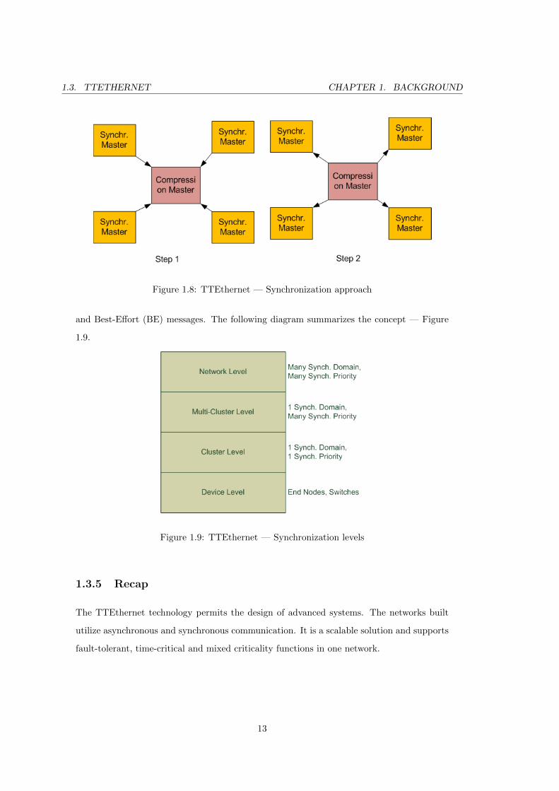
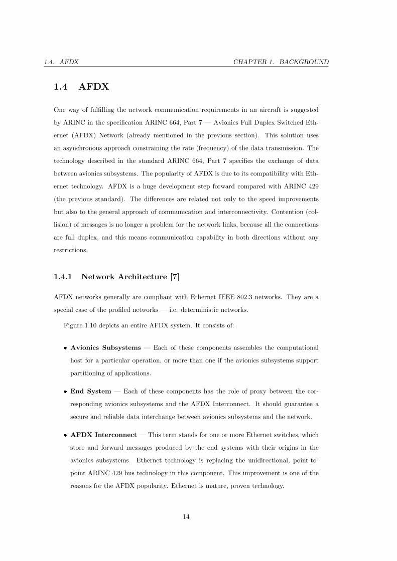
TTEthernet uses a two-step approach for the synchronization functions. In the beginning
the synchronization master nodes send protocol control frames to the compression master
nodes. The last ones to receive these frames calculate an average value for the relative arrival
times and send out a control frame in this step. The new protocol frame is announced by
sending it to the synchronization clients. The exact role of the devices is a design decision.
Most of the time the synchronization masters are the switches but it can also be the other
way around. The protocol is depicted in Figure 1.8.
There are four different layers embodied in the synchronization topology of TTEthernet
network. Three types of devices are involved in these levels: synchronization masters, syn-
chronization clients and compression masters. The first layer is the devices. In the next layer,
clusters are formed from devices (end systems and switches) that have the same synchroniza-
tion priority and synchronization domain. There is also a multi-cluster level, which adds to
the previous multiple synchronization priorities. On top of these is the network level, which
handles multiple synchronization levels with multiple priorities. Synchronization within a
cluster is done through the algorithm described above and those levels, comprising two or
more clusters (multi-cluster level), include synchronization through Rate-Constrained (RC)
12
1.3. TTETHERNET CHAPTER 1. BACKGROUND
Figure 1.8: TTEthernet — Synchronization approach
and Best-Effort (BE) messages. The following diagram summarizes the concept — Figure
1.9.
Figure 1.9: TTEthernet — Synchronization levels
1.3.5 Recap
The TTEthernet technology permits the design of advanced systems. The networks built
utilize asynchronous and synchronous communication. It is a scalable solution and supports
fault-tolerant, time-critical and mixed criticality functions in one network.
13
1.4. AFDX CHAPTER 1. BACKGROUND
1.4 AFDX
One way of fulfilling the network communication requirements in an aircraft is suggested
by ARINC in the specification ARINC 664, Part 7 — Avionics Full Duplex Switched Eth-
ernet (AFDX) Network (already mentioned in the previous section). This solution uses
an asynchronous approach constraining the rate (frequency) of the data transmission. The
technology described in the standard ARINC 664, Part 7 specifies the exchange of data
between avionics subsystems. The popularity of AFDX is due to its compatibility with Eth-
ernet technology. AFDX is a huge development step forward compared with ARINC 429
(the previous standard). The differences are related not only to the speed improvements
but also to the general approach of communication and interconnectivity. Contention (col-
lision) of messages is no longer a problem for the network links, because all the connections
are full duplex, and this means communication capability in both directions without any
restrictions.
1.4.1 Network Architecture [7]
AFDX networks generally are compliant with Ethernet IEEE 802.3 networks. They are a
special case of the profiled networks — i.e. deterministic networks.
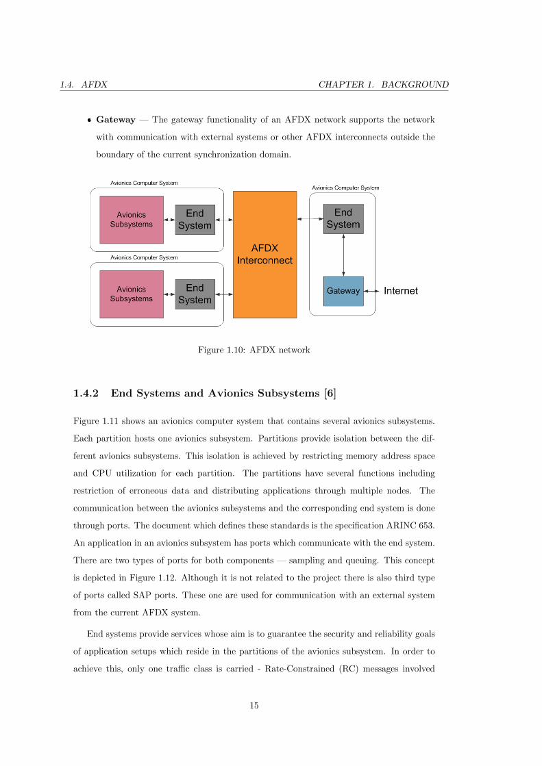
Figure 1.10 depicts an entire AFDX system. It consists of:
� Avionics Subsystems — Each of these components assembles the computational
host for a particular operation, or more than one if the avionics subsystems support
partitioning of applications.
� End System — Each of these components has the role of proxy between the cor-
responding avionics subsystems and the AFDX Interconnect. It should guarantee a
secure and reliable data interchange between avionics subsystems and the network.
� AFDX Interconnect — This term stands for one or more Ethernet switches, which
store and forward messages produced by the end systems with their origins in the
avionics subsystems. Ethernet technology is replacing the unidirectional, point-to-
point ARINC 429 bus technology in this component. This improvement is one of the
reasons for the AFDX popularity. Ethernet is mature, proven technology.
14
1.4. AFDX CHAPTER 1. BACKGROUND
� Gateway — The gateway functionality of an AFDX network supports the network
with communication with external systems or other AFDX interconnects outside the
boundary of the current synchronization domain.
Figure 1.10: AFDX network
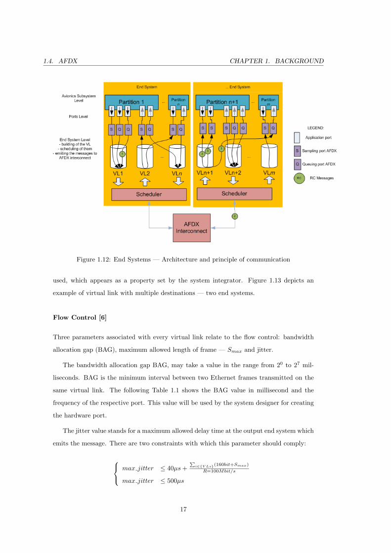
1.4.2 End Systems and Avionics Subsystems [6]
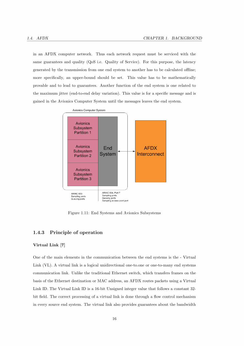
Figure 1.11 shows an avionics computer system that contains several avionics subsystems.
Each partition hosts one avionics subsystem. Partitions provide isolation between the dif-
ferent avionics subsystems. This isolation is achieved by restricting memory address space
and CPU utilization for each partition. The partitions have several functions including
restriction of erroneous data and distributing applications through multiple nodes. The
communication between the avionics subsystems and the corresponding end system is done
through ports. The document which defines these standards is the specification ARINC 653.
An application in an avionics subsystem has ports which communicate with the end system.
There are two types of ports for both components — sampling and queuing. This concept
is depicted in Figure 1.12. Although it is not related to the project there is also third type
of ports called SAP ports. These one are used for communication with an external system
from the current AFDX system.
End systems provide services whose aim is to guarantee the security and reliability goals
of application setups which reside in the partitions of the avionics subsystem. In order to
achieve this, only one traffic class is carried - Rate-Constrained (RC) messages involved
15
1.4. AFDX CHAPTER 1. BACKGROUND
in an AFDX computer network. Thus each network request must be serviced with the
same guarantees and quality (QoS i.e. Quality of Service). For this purpose, the latency
generated by the transmission from one end system to another has to be calculated offline;
more specifically, an upper-bound should be set. This value has to be mathematically
provable and to lead to guarantees. Another function of the end system is one related to
the maximum jitter (end-to-end delay variation). This value is for a specific message and is
gained in the Avionics Computer System until the messages leaves the end system.
Figure 1.11: End Systems and Avionics Subsystems
1.4.3 Principle of operation
Virtual Link [7]
One of the main elements in the communication between the end systems is the - Virtual
Link (VL). A virtual link is a logical unidirectional one-to.one or one-to-many end systems
communication link. Unlike the traditional Ethernet switch, which transfers frames on the
basis of the Ethernet destination or MAC address, an AFDX routes packets using a Virtual
Link ID. The Virtual Link ID is a 16-bit Unsigned integer value that follows a constant 32-
bit field. The correct processing of a virtual link is done through a flow control mechanism
in every source end system. The virtual link also provides guarantees about the bandwidth
16
1.4. AFDX CHAPTER 1. BACKGROUND
Figure 1.12: End Systems — Architecture and principle of communication
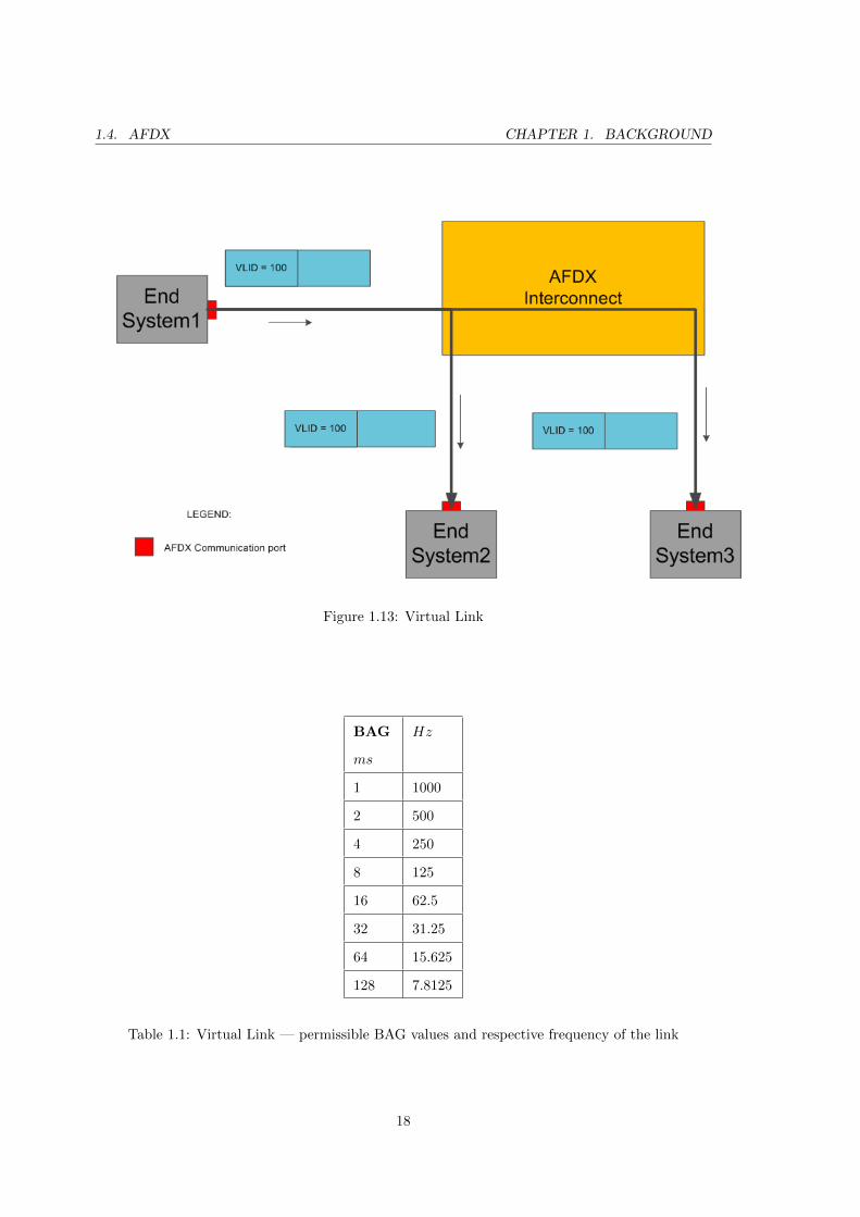
used, which appears as a property set by the system integrator. Figure 1.13 depicts an
example of virtual link with multiple destinations — two end systems.
Flow Control [6]
Three parameters associated with every virtual link relate to the flow control: bandwidth
allocation gap (BAG), maximum allowed length of frame — Smax and jitter.
The bandwidth allocation gap BAG, may take a value in the range from 20 to 27 mil-
liseconds. BAG is the minimum interval between two Ethernet frames transmitted on the
same virtual link. The following Table 1.1 shows the BAG value in millisecond and the
frequency of the respective port. This value will be used by the system designer for creating
the hardware port.
The jitter value stands for a maximum allowed delay time at the output end system which
emits the message. There are two constraints with which this parameter should comply:
max jitter ≤ 40µs+∑
i∈{V Ls}(160bit+Smax)
R=100Mbit/s
max jitter ≤ 500µs
17
1.4. AFDX CHAPTER 1. BACKGROUND
Figure 1.13: Virtual Link
BAG
ms
Hz
1 1000
2 500
4 250
8 125
16 62.5
32 31.25
64 15.625
128 7.8125
Table 1.1: Virtual Link — permissible BAG values and respective frequency of the link
18
1.4. AFDX CHAPTER 1. BACKGROUND
where R is the medium bandwidth of the network and V Ls are all the virtual links in
the system.
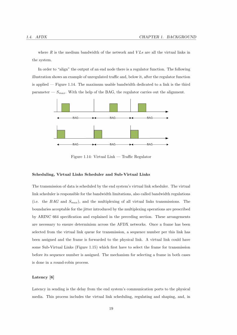
In order to “align” the output of an end node there is a regulator function. The following
illustration shows an example of unregulated traffic and, below it, after the regulator function
is applied — Figure 1.14. The maximum usable bandwidth dedicated to a link is the third
parameter — Smax. With the help of the BAG, the regulator carries out the alignment.
Figure 1.14: Virtual Link — Traffic Regulator
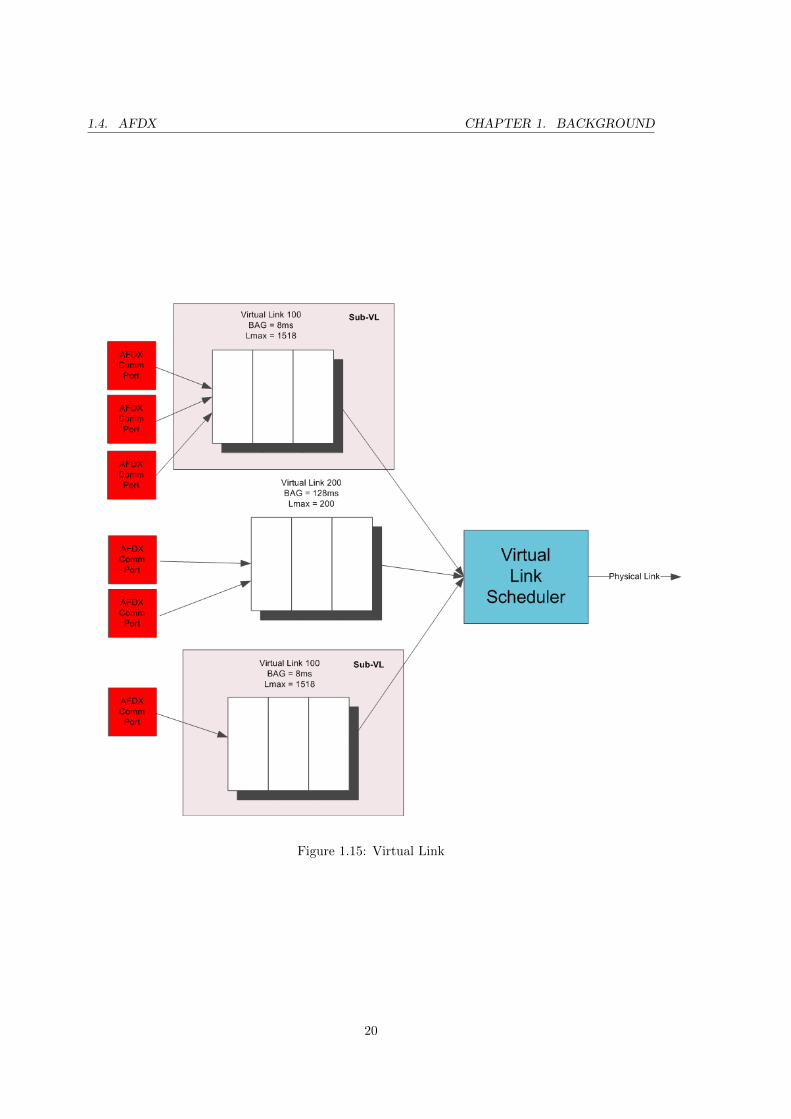
Scheduling, Virtual Links Scheduler and Sub-Virtual Links
The transmission of data is scheduled by the end system’s virtual link scheduler. The virtual
link scheduler is responsible for the bandwidth limitations, also called bandwidth regulations
(i.e. the BAG and Smax), and the multiplexing of all virtual links transmissions. The
boundaries acceptable for the jitter introduced by the multiplexing operations are prescribed
by ARINC 664 specification and explained in the preceding section. These arrangements
are necessary to ensure determinism across the AFDX networks. Once a frame has been
selected from the virtual link queue for transmission, a sequence number per this link has
been assigned and the frame is forwarded to the physical link. A virtual link could have
some Sub-Virtual Links (Figure 1.15) which first have to select the frame for transmission
before its sequence number is assigned. The mechanism for selecting a frame in both cases
is done in a round-robin process.
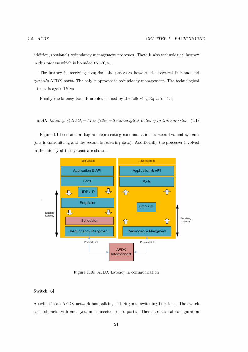
Latency [6]
Latency in sending is the delay from the end system’s communication ports to the physical
media. This process includes the virtual link scheduling, regulating and shaping, and, in
19
1.4. AFDX CHAPTER 1. BACKGROUND
Figure 1.15: Virtual Link
20
1.4. AFDX CHAPTER 1. BACKGROUND
addition, (optional) redundancy management processes. There is also technological latency
in this process which is bounded to 150µs.
The latency in receiving comprises the processes between the physical link and end
system’s AFDX ports. The only subprocess is redundancy management. The technological
latency is again 150µs.
Finally the latency bounds are determined by the following Equation 1.1.
MAX Latencyi ≤ BAGi +Max jitter + Technological Latency in transmission (1.1)
Figure 1.16 contains a diagram representing communication between two end systems
(one is transmitting and the second is receiving data). Additionally the processes involved
in the latency of the systems are shown.
Figure 1.16: AFDX Latency in communication
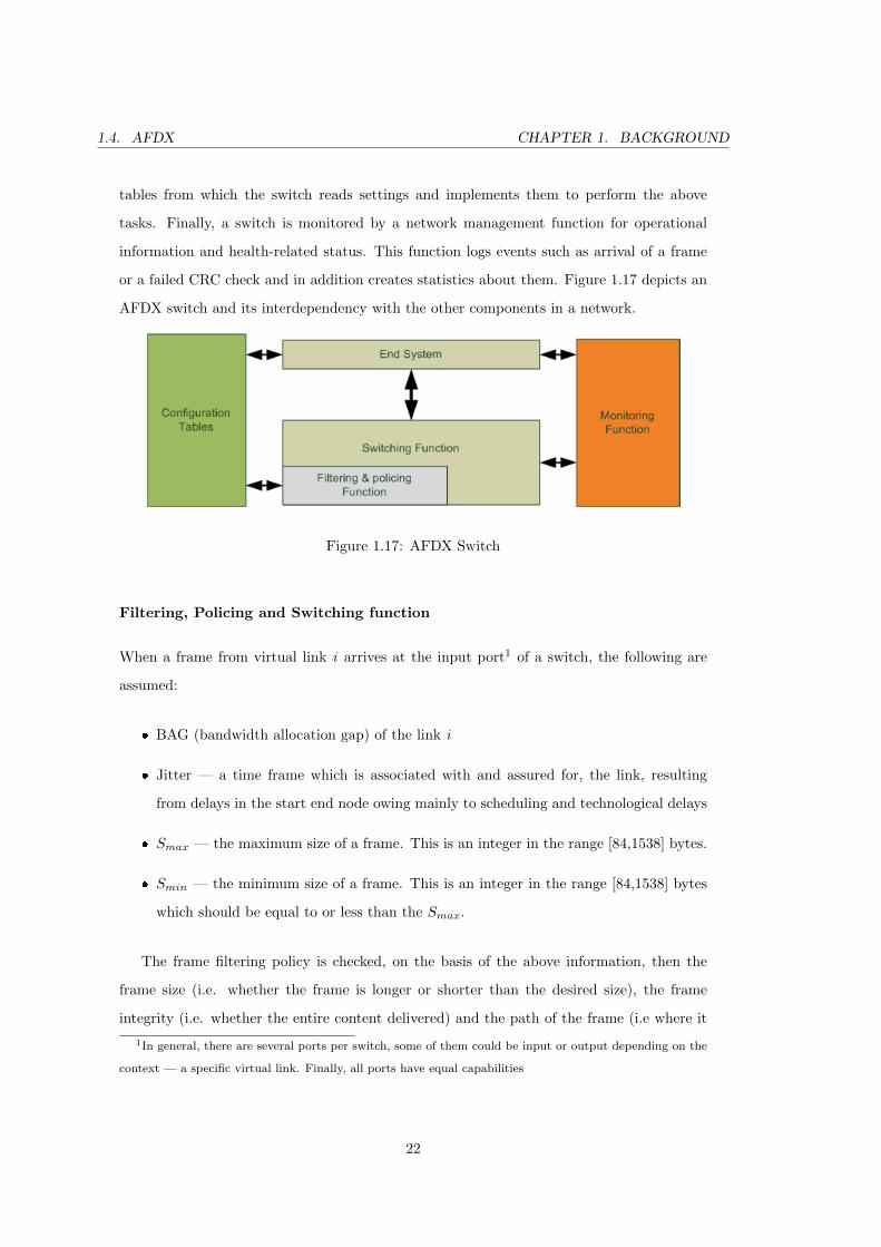
Switch [6]
A switch in an AFDX network has policing, filtering and switching functions. The switch
also interacts with end systems connected to its ports. There are several configuration
21
1.4. AFDX CHAPTER 1. BACKGROUND
tables from which the switch reads settings and implements them to perform the above
tasks. Finally, a switch is monitored by a network management function for operational
information and health-related status. This function logs events such as arrival of a frame
or a failed CRC check and in addition creates statistics about them. Figure 1.17 depicts an
AFDX switch and its interdependency with the other components in a network.
Figure 1.17: AFDX Switch
Filtering, Policing and Switching function
When a frame from virtual link i arrives at the input port1 of a switch, the following are
assumed:
� BAG (bandwidth allocation gap) of the link i
� Jitter — a time frame which is associated with and assured for, the link, resulting
from delays in the start end node owing mainly to scheduling and technological delays
� Smax — the maximum size of a frame. This is an integer in the range [84,1538] bytes.
� Smin — the minimum size of a frame. This is an integer in the range [84,1538] bytes
which should be equal to or less than the Smax.
The frame filtering policy is checked, on the basis of the above information, then the
frame size (i.e. whether the frame is longer or shorter than the desired size), the frame
integrity (i.e. whether the entire content delivered) and the path of the frame (i.e where it
1In general, there are several ports per switch, some of them could be input or output depending on the
context — a specific virtual link. Finally, all ports have equal capabilities
22
1.4. AFDX CHAPTER 1. BACKGROUND
is to be delivered). If a frame does not comply with these conditions it is discarded and the
monitoring function is modified according to the information for rejection of a frame.
The next step to be performed is the policing algorithm on the Destination Address basis
of a virtual link. The traffic policing has the task of regulating the bandwidth usage or in
other words the traffic “injected” into a network. This is done by one of two algorithms:
Byte-based traffic policing or Frame-based traffic policing. Both have the same function but
the measurement in one case is expressed in bits per second and in the other as frames per
seconds. A switch may implement both of them. The algorithm implements the following
function for the “account” ACi for the virtual link V Li:
Simax.
(1 +
J iswitch
BAGi
)(1.2)
In the case where the switch is using the frame-based policing algorithm, the following
applies. If a frame ACi is greater than Simax, then the frame is accepted and frame ACi
is debited by Simax. If this condition is not obeyed, the frame is discarded, and ACi is not
changed. A notification is sent to the monitoring functions. In this way the containment
function of the network is ensured and implemented. Since an end system which is corrupted
does not disturb the other network traffic, its frames are not accepted furthermore by a
switch.
The choice of policing algorithm is based on the Destination Address of a virtual link.
There are two types of relationship between MAC destination addresses and ACi. First, one
ACi could service only one Destination Address (MAC). Second, this could be implemented
for several destinations. In this way the propagation of faulty frames is prevented. A
shared virtual link (used by many applications in the end node) is part of only one ACi
account. This technique could be beneficial for applications distributed across multiple
partitions and sharing one communication virtual link. This capability will compromise
the segregation between the respective virtual links, as well as eliminating the required
bandwidth guarantees.
The switching function obtains the Destination Address from the configuration tables
and then performs the forwarding. Conditions which are checked, when this action is taken,
are the status of the destination port (i.e. whether the buffer in the port contains enough
available memory) and the “max delay” of the frame (i.e. the delay for a frame calculated
using the formula compared with the one set in the configuration).
23
1.4. AFDX CHAPTER 1. BACKGROUND
The switching capabilities include a prioritization mechanism dependant on the Desti-
nation Address, with two priority classes. These are High priority and Low priority. The
priority level is configured in the configuration tables of the switch. For each output port,
frames with higher priority are sent a priori, and those of lower priority class are pre-empted
and delayed.
1.4.4 Recap
The AFDX technology combines concepts taken from an asynchronous network model with
well-known Ethernet technology. At the physical level AFDX has star topology with main
devices — the switches. In addition, the network is profiled on a frame level. All connections,
addressing tables and bandwidth requirements are well-known in advance. At protocol level
there is a notation called virtual link — a point-to-point or multicast connection between end
systems. Again, the network is profiled, and the addressing and bandwidth values are known
a priori. Moreover, the network is deterministic, with latency of each connection known at
the design stage. The traffic shaping and regulating mechanisms in the end system and
those in the switch (i.e. traffic policing) help to guarantee the latency, jitter and bandwidth
for each virtual link, ensuing the required QoS.
24
1.5. INTEGRATION CHAPTER 1. BACKGROUND
1.5 Integration
In this chapter we have introduced two technologies — TTEthernet and AFDX. As can be
seen, TTEthernet is compatible with AFDX and not the other way around. This is due to
TTEthernet supporting integration of different traffic classes. AFDX has only one traffic
class even though the switches may be able to support these capabilities.
In our work we rely on the TTEthernet. But as much of it is mature and proven
technology, we will use the details of AFDX when it comes to elaborative description of
the configurations. First, we will explain the scope of our problem in an environment
which contains properties fully compliant with AFDX, and afterwards we will extend the
configuration to include properties related to and available only in TTEthernet.
25
Chapter 2
Motivation
2.1 Introduction
In this chapter we provide a motivation for the problem featured in this project. First, we
will introduce:
� the hardware architecture
� the software architecture
� and the application model related to our problem.
Afterwards, the problem is described in the terms of the the constraints introduced and
the technologies discussed in the previous chapter.
Finally, the chapter also includes additional assumptions.
26
2.2. HARDWARE ARCHITECTURE CHAPTER 2. MOTIVATION
2.2 Hardware Architecture
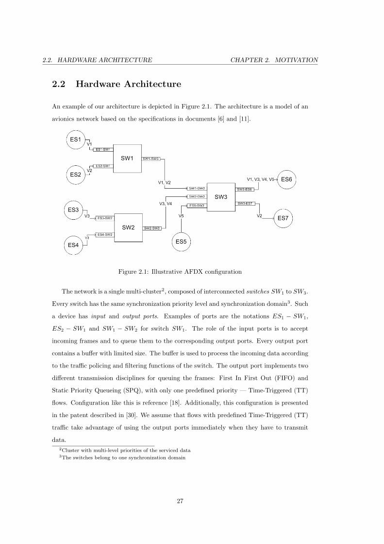
An example of our architecture is depicted in Figure 2.1. The architecture is a model of an
avionics network based on the specifications in documents [6] and [11].
Figure 2.1: Illustrative AFDX configuration
The network is a single multi-cluster2, composed of interconnected switches SW1 to SW3.
Every switch has the same synchronization priority level and synchronization domain3. Such
a device has input and output ports. Examples of ports are the notations ES1 − SW1,
ES2 − SW1 and SW1 − SW2 for switch SW1. The role of the input ports is to accept
incoming frames and to queue them to the corresponding output ports. Every output port
contains a buffer with limited size. The buffer is used to process the incoming data according
to the traffic policing and filtering functions of the switch. The output port implements two
different transmission disciplines for queuing the frames: First In First Out (FIFO) and
Static Priority Queueing (SPQ), with only one predefined priority — Time-Triggered (TT)
flows. Configuration like this is reference [18]. Additionally, this configuration is presented
in the patent described in [30]. We assume that flows with predefined Time-Triggered (TT)
traffic take advantage of using the output ports immediately when they have to transmit
data.
2Cluster with multi-level priorities of the serviced data3The switches belong to one synchronization domain
27
2.2. HARDWARE ARCHITECTURE CHAPTER 2. MOTIVATION
The inputs and outputs of the network architecture, called end systems, are denoted with
ES1 to ES7. Every end system is connected to exactly one switch port and each switch
port is connected to at most one end system. An end system can emit and receive data
simultaneously. The details describing the transmission flows of data structures and their
behaviour are given in section 2.3
The links between any switch and end system are full duplex Ethernet. This eliminates
the indeterminism of the underlying CSMA-CD Ethernet technology.
28
2.3. SOFTWARE ARCHITECTURE CHAPTER 2. MOTIVATION
2.3 Software Architecture
We have decided on a specific software architecture that runs on every end system node.
The architecture is in accordance with the specification in reference [6].
Our software architecture has the following functions:
� fetching data from a local bus
� constructing frames dependant on and restricted by the shaping unit4 of the end system
� scheduling of the frames for sending
� transmission of the frames
� acceptance of frames
When the data is available and fetched from the bus it is transformed and wrapped
in a virtual link before is sent as a sequence of frames. Only one end system can be the
source of a particular virtual link. Thus, all virtual links describe in an explicit way the
end-to-end communication. The sample configuration shown in Figure 2.1 contains virtual
links denoted by V1 to V5. As described in the ARINC-664 standard [6], the virtual link
is a concept based on a virtual communication channel where all communication flows are
statically defined offline. There are two types of virtual links:
� unicast (e.g. V1 with path ES1 − SW1 − SW3 − ES6). This is a case where a virtual
link has single start and end points
� multicast (e.g.V2 with subpaths ES2−SW2−SW3−ES6 and ES2−SW2−SW3−ES7).
In this example a virtual link again has a single starting point but more than one end
point. The data is cloned (from the traffic policing unit of a switch) in an appropriate
manner when the link is forked, without any extra timing penalty.
By definition, every virtual link is implemented with two parameters — BAG (Bandwidth
Allocation Gap) and minimum and maximum length (Sminand Smax). BAG is the minimum
delay between two full consecutive emissions of data in a virtual link. This means that a
virtual link that has to transmit an amount of data S must do it for an interval of time
4The constraints are related to proper time of emitting of a message and the size of it
29
2.3. SOFTWARE ARCHITECTURE CHAPTER 2. MOTIVATION
equal to BAG. The pair (Smin, Smax) determines the minimum and the maximum amount
of data respectively for transmission in the ingress node of a virtual link. (Obviously this
node is an end system). This means that, no matter how many transmissions are performed
in a period BAG5, the sum of them should not exceed S ≤ Smax. Alternatively, if there
is only one transmission, then S = Smax. These limitations are guaranteed by the shaping
unit software of the end system and the traffic policing unit in every switch input port in the
path of the link. Both properties will be taken into account when the virtual link scheduling
is performed in the end systems and the corresponding switches in the path.
We consider every virtual link to transmit a single predefined, dedicated service class of
frames according the specification in reference [11]. These can be Rate-Constrained (RC),
Time-Triggered (TT) and Best-Effort (BE) messages6. The architecture shown in Figure
2.1 contains five virtual links and their network classes could be 2 Time-Triggered (TT) —
V1, V4, 2 Rate-Constrained (RC) — V2, V3 and 1 Best-Effort (BE) — V5.
It is worth mentioning that the TCP/IP stack in the AFDX end systems is implemented
in the NIC 7 adapter. This is done in order to save limited CPU and memory resources
in the avionics subsystems partitions 8. The static configuration of the AFDX networks
described does not require many components of the traditional TCP/IP implementations
like ICMP, ARP and etc. Thus, the implementation highlights performance, with short
response times regarding the number of the emitted frames per any end system [19], and
limited other functionality.
5The restrictions for the BAG values are presented in the Background chapter, Ch. 16See the Background chapter, Ch. 17Network Interface Controller8The applications are hosted at this level
30
2.4. APPLICATION MODEL CHAPTER 2. MOTIVATION
2.4 Application model
We model an application A as a set of directed, acyclic graphs G(V,E) ∈ A. A node
Pmi ∈ V (m ∈ [1, n])9 describes a process of sending out data from a particular switch or
end system to another switch or end system within the boundary of a particular graph m.
An edge emij ∈ E from Pmi to Pm
j indicates that the output of Pmi is the input for Pm
j and it
represents a communication link from the hardware configuration. We define that a graph
m dimensions are equal to a virtual link paths — P. Moreover the application model makes
it possible to intersect the hardware configuration and to represent multiple virtual links
with the same ingress node to different independent nodes from the graphs. The concept
notation is depicted in Figure 2.2:
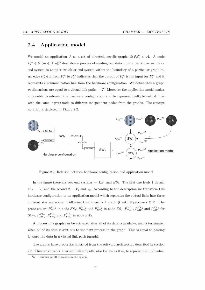
Figure 2.2: Relation between hardware configuration and application model
In the figure there are two end systems — ES1 and ES2. The first one feeds 1 virtual
link — V1 and the second 2 — V2 and V3. According to the description we transform this
hardware configuration to an application model which separates the virtual links into three
different starting nodes. Following this, there is 1 graph G with 9 processes ∈ V. The
processes are PV L1
ES1in node ES1; PV L2
ES2and PV L3
ES2in node ES2; PV L1
SW1, PV L2
SW1and PV L3
SW1for
SW2; PV L1
SW2, PV L2
SW2and PV L3
SW3in node SW3.
A process in a graph can be activated after all of its data is available, and is terminated
when all of its data is sent out to the next process in the graph. This is equal to passing
forward the data in a virtual link path (graph).
The graphs have properties inherited from the software architecture described in section
2.3. Thus we consider a virtual link subpath, also known as flow, to represent an individual
9n — number of all processes in the system
31
2.4. APPLICATION MODEL CHAPTER 2. MOTIVATION
graph Gm. Overall each virtual link has minimum inter-arrival time at the ingress end system
node, denoted with Tm and maximum release jitter at the same node, denoted with Jm. The
maximum inter-arrival time is another way to denote the BAG property of a virtual link.
From the other side, the maximum jitter Jm stands for a function which accumulates the
maximum time allowed for subtranmissions (if they exist) when a virtual link transmits
partial data S (Smin < S < Smax) in multiple emissions.
There is contention between the different graphs for the hardware resources — e.g. every
switch output port or end system can emit only the data of a particular process Pm per unit
of time. Thus the scheduling policy for each process in the switch nodes is FIFO and for the
end nodes the graphs are scheduled in a round-robin sequence. A process Pm communication
with another process mapped to the same end system is not modelled explicitly and is not
considered as “influence”. Evidence for this is the intersecting application model. The
maximum process time of Pm on any node i from the path Pm is denoted as Cmi . The
dependencies for this process time and the assumptions behind it are given in the section
2.5.
32
2.5. TECHNOLOGICAL NOTATIONS CHAPTER 2. MOTIVATION
2.5 Technological notations
The application model in section 2.4 introduced the required notations. We adhere to them
as follows:
Every edge eij in the application transmits any size of data for a time value L = Lmin =
Lmax = 16µs. This constant is relevant to the technological delay caused by the full duplex
Ethernet links in the hardware system.
The time taken by a process Pm for crossing node i (described as Pmi in section 2.4) is
Cim = Smax/R, where Smax is the maximum length of the emitted data (by a virtual link)
and R the hardware-limited bandwidth of the network (usually 100 Mbit/s). Alternatively
the transmission time through the node can vary when the virtual link transmits less data
S (Smin < S < Smax).
33
2.6. PROBLEM FORMULATION CHAPTER 2. MOTIVATION
2.6 Problem formulation
We shall now consider statically predefined Time-Triggered (TT) messages in the network
applications that we are researching. These are compatible and integrated with the models
and the configurations described so far in sections 2.2, 2.3 and 2.4. At the same time
the application A is handling Rate-Constrained (RC) traffic. The following factors are
considered for the Time-Triggered (TT) traffic:
� Static messages take precedence over all other network traffic.
� Statically defined messages have hard deadlines denoted with Dm, where m ∈ [1, n]
and Dm < Tm (Tm is the period of a message).
� These messages occupy predefined time-segments in their paths in the corresponding
graphs G. Therefore the point of time at which every Time-Triggered (TT) process
Pmi
TT passes every node in its path Pm can be identified exactly.
� This type of traffic uses synchronized switches and end systems in order to complete
the synchronization between all the Time-Triggered (TT) traffic. Any co-existence of
Time-Triggered (TT) and Rate-Constrained (RC) traffic in any particular end system
is impossible. If it is, the Rate-Constrained (RC) traffic can also be “synchronized” by
mapping it to the Time-Triggered (TT) traffic. Thus the application model does not
change. The presence of Time-Triggered (TT) traffic adds extra graphs on the top of
the existing ones.
� The Time-Triggered (TT) traffic segments are created offline and have an impact over
the rest of the traffic by preventing the communication of the Rate-Constrained (RC)
traffic from progressing during the transmission of the higher priority traffic.
In scenario I we consider a set s of defined Gs graphs (s ∈ [1, n]) executing prede-
fined Time-Triggered (TT) traffic. There is a function FTT : V → VoptRC which gives the
optimized result for the rest n − s Rate-Constrained (RC) graphs Gn−s. This function de-
terminates the scope for carrying the Time-Triggered (TT) traffic over the network and is
calculated offline by the system designer. We define a set of rules S which have to be fulfilled
or are considered as advisable with regard to the Rate-Constrained (RC) traffic.
34
2.6. PROBLEM FORMULATION CHAPTER 2. MOTIVATION
Alternatively, in scenario II, the n−s Rate-Constrained (RC) graphs Gn−s are inspected
and the virtual link parameters for Rate-Constrained (RC) are optimized. This is done
through a function FRC : V → VoptRC . This time the Time-Triggered (TT) traffic is not
changed at all. In this case the set of rules S are related to non-changeable Time-Triggered
(TT) traffic.
Our problem formulation is as follows:
� As input we have an application A with a set of graphs — Time-Triggered (TT) and
Rate-Constrained (RC).
� The available parameters data for every Time-Triggered (TT) graph are
< T,D, Smax, Smin, start− uptime >
� The available parameters for every Rate-Constrained (RC) graph are
< T = BAG,Smax, Smin >
� The goals of the application are set through S and they respect in scenario I the
opportunity to build the “best results” for constraints related to Rate-Constrained
(RC) traffic and in scenario II for limitations related to Time-Triggered (TT) traffic.
The ”best results” to which we point in both scenarios are the shortest end-to-end
delay times for the Rate-Constrained (RC) traffic, since the Time-Triggered (TT)
delays can vary but are always expected to be as they are designed. Moreover the
unpredictability of the Rate-Constrained (RC) traffic is the result of the dedicated
service class10 of this kind of messages and a satisfactory result is one that shows the
highest bounds of these end-to-end delays.
With the term “end-to-end delay” time for a given message we define the time needed
for crossing the message’s own ingress node, all links and switches in the network exactly,
before the message is delivered to the destination node of the network. This time could be
an absolute or relative value.
In conclusion we will determinate configuration ψ =< F ,S > for which the optimal
deviation F of the corresponding graphs is chosen for a set of rules S and the current
scenario.10This is explained previously in the Background chapter
35
2.6. PROBLEM FORMULATION CHAPTER 2. MOTIVATION
From now on, our main focus in the next chapters will be to study and analyse Rate-
Constrained (RC) traffic, to work out an appropriate approach for determination of its end-
to-end delays and to apply the result to both scenarios as they were described. This process
will include exploration of the work already done in the area and consequently its extension.
We will reckon the problem as solved if we apply and show results for the methods developed
to different hardware and software configurations which support the models described so far.
36
Chapter 3
End-to-end delay analysis
3.1 Introduction
In this chapter we will analyse the core problem of this thesis project, i.e. how the timing
delay of Rate-Constrained (RC) messages can be determinated in terms of the configurations
examinated and described in the Motivation chapter, Ch.2.
A survey of all existing methods in the literature compliant with the problem will be
shown first. Second, we do preliminary analysis of the delays and show where exactly the
delays have dynamic/undefined parts which have to be calculated.
Afterwards, we adopt an analysis based on the Trajectory approach[28], [29] for the
purpose of our task.
37
3.2. STATE OF THE ART CHAPTER 3. END-TO-END DELAY ANALYSIS
3.2 State Of The Art
The AFDX network is a new innovative research discipline which has been studied from the
community recently. The area in which we are interested, is related to the produced end-
to-end delays of the flows. The scrupulous exploration of the determinism of these delays
is used for certification purposes. Different approaches have been proposed to analyse the
end-to-end delays.
3.2.1 Network Calculus
The network calculus approach is a traditional approach described in many papers. The
method is based on network theories. It is used to describe the arrival curves of the virtual
links traffic and further to estimate the minimal service offered by the network switches. The
calculus gives the latency of any network entity (virtual link) and, for those with queueing
capabilities (switches), the queue size bound in bits divisible by Smin of any virtual link.
If the service curve of the switches is designated by β and the network arrival curve of the
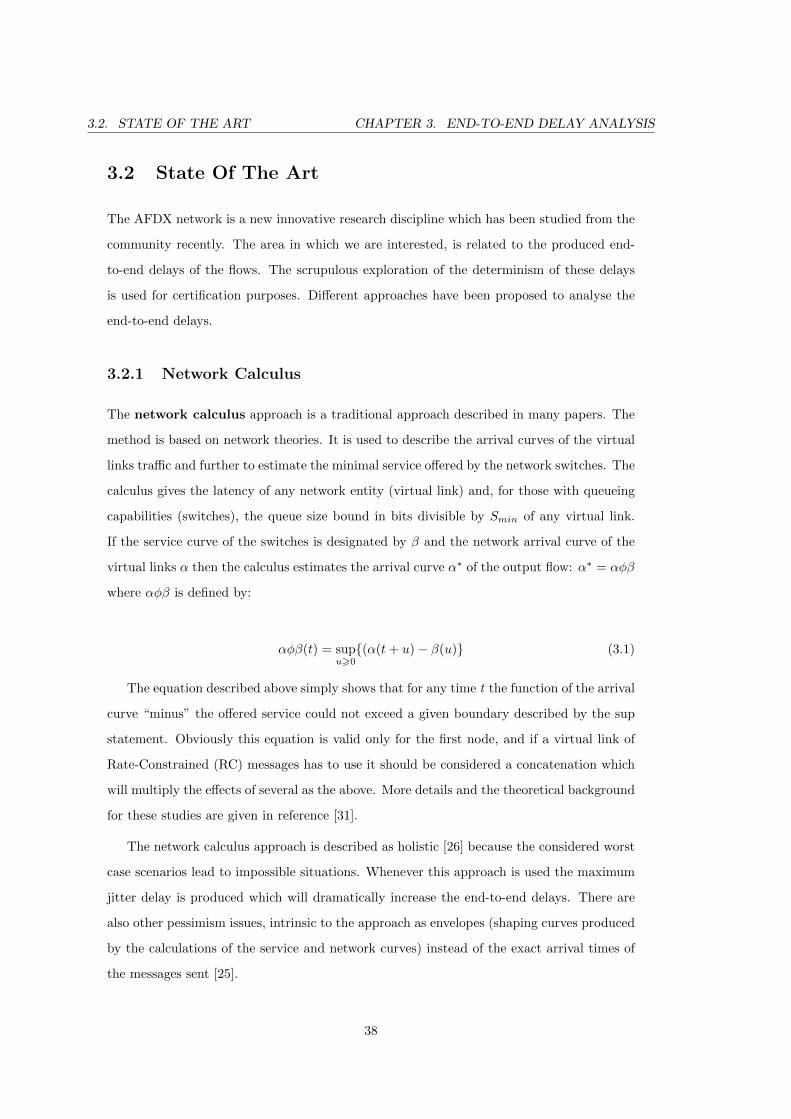
virtual links α then the calculus estimates the arrival curve α∗ of the output flow: α∗ = αφβ
where αφβ is defined by:
αφβ(t) = supu>0{(α(t+ u)− β(u)} (3.1)
The equation described above simply shows that for any time t the function of the arrival
curve “minus” the offered service could not exceed a given boundary described by the sup
statement. Obviously this equation is valid only for the first node, and if a virtual link of
Rate-Constrained (RC) messages has to use it should be considered a concatenation which
will multiply the effects of several as the above. More details and the theoretical background
for these studies are given in reference [31].
The network calculus approach is described as holistic [26] because the considered worst
case scenarios lead to impossible situations. Whenever this approach is used the maximum
jitter delay is produced which will dramatically increase the end-to-end delays. There are
also other pessimism issues, intrinsic to the approach as envelopes (shaping curves produced
by the calculations of the service and network curves) instead of the exact arrival times of
the messages sent [25].
38
3.2. STATE OF THE ART CHAPTER 3. END-TO-END DELAY ANALYSIS
3.2.2 Grouping technique
Another approach to the analysis of end-to-end delays is the grouping technique. This
technique is used as improvement of the network calculus approach. It consists of a concept
for grouping the virtual links which share at least one edge 11. The key point is that the
frames of these virtual links are serialized after exiting the first multiplexer (an end node
or a switch) and thus they do not have to be serialized again in the following multiplexers.
This utilizes the bandwidth and minimizes the blocking interdependency of the flows when
they have to use common hardware resources.
This approach is used and mentioned in [26] and [25].
3.2.3 Simulation approach
The simulation approach is designed to determinate experimentally the maximum upper
bounds on a set of scenarios, which will eventually be “sharper” than network calculus
calculations. This is so because network calculus is a generalization and derives sure upper
bounds on the delays contrariwise the simulation approach, which tests only limited and
known cases.
The simulation strategy is used in [20] and [24]. The approach described has discussions
about certain parameters which are taken into account. These are related to the virtual link
emission strategy. More specifically these are options that:
� decide whether the frames can be generated periodically, using the BAG as a period,
OR frames can be generated sporadically, using the BAG (Bandwidth Allocation Gap,
equal to the period Tm) as a minimum inter-emission time
� experiment with the phasing between virtual links (a synchronized one, in which the
first frame of every virtual link is transmitted at the same time, OR a desynchronized
one, in which we assign a phase randomly distributed between 0 and its BAG) to each
virtual link
� try different frame sizes such as e.g. the minimum length for every frame of every
virtual link, the maximum length for every frame of every virtual link, the average
length between the minimum and the maximum ones for every frame of every virtual
11In our case this is when emij = elij and where m,l ∈ [1, n], n — all graphs G in the application A
39
3.2. STATE OF THE ART CHAPTER 3. END-TO-END DELAY ANALYSIS
link, or a random length between the minimum and the maximum ones for every
frames of every virtual link
On the other hand the simulation approach can describe generic models of predefined
configurations. These configurations are examined for influence in between the composed
virtual links. As result the simulation space is reduced. Moreover larger configurations can
be represented as a composition of such predefined models. In this way larger architectures
can be simplified and they tend to be simulated more easily. This extension of the approach
is considered in [24].
3.2.4 Time automata
There is also a timed automation modelling approach based on timed automata. It
is suitable only for small configurations because the models used lead to a combinatorial
explosion in larger configurations and they become unsolvable. This method consists of the
exploration of all the possible states of a system and will thus determine an exact worst-case
end-to-end delay. It implies computing whether a property, expressed by a timed logic,
is verified or not. A timed automaton is a finite automaton with a set of clocks with time
variables that are increased uniformly in the time. The model checking approach determines
an exact worst-case end-to-end delay in the corresponding scenario, since it explores all the
possible states of the system. The composition of the time is obtained in a synchronous
way. This means if two actions lead to one which could be performed, then the time for
both is considered. Performing the transitions does not cost time, but conversely the time
is running in the nodes. Thus reachability analysis is performed by model-checking and this
means that a property is verified if it is reachable from the initial configuration.
If we consider a system with 5 virtual link flows and 3 intersecting switches, their compo-
nents can be modelled by automata as in the following equation. The global system model
is obtained by composition of all automata:
System = Switch1‖Switch2‖Switch3‖F0‖F1‖F2‖F3‖F4 (3.2)
These analyses are implemented in [20]. In the same work some techniques are suggested
which have as their the reduction of the overload of the calculations, e.g using a generalization
approach which takes into account the separate modules of the system, already calculated.
40
3.2. STATE OF THE ART CHAPTER 3. END-TO-END DELAY ANALYSIS
3.2.5 Stochastic network calculus
The next technique proposed is stochastic network calculus. This method gives an
evaluation for the distribution of end-to-end delays of a given flow in the configuration. The
distribution obtained is pessimistic if it is compared with the real behaviour of a network
observed through simulation. On the other hand, the pessimism is less than the upper
bounds obtained by a network calculus approach.
We will describe briefly the background configuration for the approach. Every switch
output port has to aggregate traffic with its capacity at a constant rate c which is the
capacity of the output link (100 Mbit/s). Every single flow is shaped separately at network
access level by the BAG (Bandwidth Allocation Gap). This corresponds to a network subject
to EF PHB (Expedited Forwarding Per-Hop Behaviour) service of DiffServ (Differentiated
Services) [32]. The nodes, in this case the switch output ports, are denoted as PSRG (Packet
Scale Rate Guarantee) nodes and the EF traffic in a node is served with a rate independently
of any other traffic transiting through the same node.
A node is PSRG (c, e), where c is the guaranteed rate with latency (error rate) e. If we
denote the departure of nth packet of the EF aggregate flow, in order of arrivals as dn , then
dn satisfies the inequality: dn ≤ fn + e where fn is calculated recursively as f0 = 0 and
fn = max {an,min {dn−1, fn−1}}+lnc, n ≥ 1 (3.3)
where the nth packet arrives at time an with ln bits.
The further analysis of Vojnovic and Le Boudec [21], [22] of networks with EF PHB
services are used to calculate the distribution of the waiting time for each switch. The
calculations are based on the probability of bound buffer overflow in the switch output port.
The authors of the above-mentioned references made several assumptions and set out proof
that identify the AFDX traffic flows as the one modelled in sections 2.2, 2.3 and 2.4 and
the background configuration above described.
In order to determinate the waiting delay in the output port of the switch, the waiting
delay at the moment of the arrival of frame f needs to be known. This is called compli-
mentary distribution of the backlog12. There is a probability that the size of all frames in
the output buffer including f exceeds level b. This kind of probability is denoted with PA
12Backlog is the quantity of bits that are held inside the output port
41
3.2. STATE OF THE ART CHAPTER 3. END-TO-END DELAY ANALYSIS
and is named palm probability. P(d(0) > 0) is the probability that d(0) (denotes the delay
through a node of a frame arriving in the node at time 0) exceeds u. In order to calculate
the probability of the end-to-end delay for a given virtual link, we compute it for different
values of u. At the end we consider:
P(d(0) = u) = P(d(0) > u− 0.5)− P(d(0) > u+ 0.5) (3.4)
The approach described is used in [23] and [24].
Another known and suggested method related to this approach is described in [24]. The
theory in this resource is based on the same principles as those described above. Starting
from this point, the main discussion is how to apply the probabilistic network analysis to a
chain of nodes and more especially in a sequence that is equal to the path of a virtual link.
The discussion of the approach ends with results achieved in Equation 3.4 transformed to
multihop flows.
3.2.6 Heuristic optimizations
In order to obtain more qualitative results several heuristic optimization methods are
mooted in [25]. Among the suggested alternatives are a tentative Alpha-Beta-assisted brute-
force approach, genetic algorithms and priority experiments. The paper shows significant
improvements in end-to-end delays and the availability of the queueing buffers while series
of genetic algorithms is used.
In the following paragraph we are describe a genetic optimization method related to
assigning a priority to a virtual link. By default the priority of the virtual links is not a part
of the specification described in [6]. This work uses several ways for spreading out of the
priorities but the important conclusion in it is the ability to assign one of only two priority
classes to a virtual link - low priority and high priority. Setting priorities should play only a
balancing role for an AFDX network. The standard [6] characterizes the AFDX networks as
“profiled networks” and more specifically as “deterministic networks”. The latter signifies
the paramount quality of the timed services offered. Thus all virtual links should respect
the same jitter and latency delay constraints independent of their priority class.
The process of assigning priority to virtual links is described in several steps. Firstly
an approach is tried where these values are randomly assigned. The problem in this case is
42
3.2. STATE OF THE ART CHAPTER 3. END-TO-END DELAY ANALYSIS
the unpredictability of the approach. Some segments of the network could show very low
performance as result of the technique.
As a second step the network calculus model is updated, so the derived values regarding
the influence of the priorities are correct. The assumption that only two priorities exist is
turned into a combinatorial problem (e.g. if there are 1007 virtual links, there should be
21007 combinations of priority assignment). Some of the cases are insignificant but they still
have some influence.
Finally the process of searching for an optimal minimum for the end-to-end delays is
carried on a “good” configuration. Several of these configuration and the corresponding
results can give the optimal solution when a Alpha-Beta reduction in a binary-tree is used.
The same resource [25] proposes optimization using genetic algorithms that are a subset
of the evolutionary algorithms. Basically the genetic algorithms represent points in the
optimization space by individuals, themselves represented by genes, and iterate generations
of population with reproduction and “natural” selection.
3.2.7 Stochastic upper bounds for heterogeneous flows
A step forward in the priority assignment of virtual flows is the work repeated in [18]. The
results presented here are for flows with static priorities in a configuration that uses static
priority queuing. The analyses are based on the stochastic network approach and include
an extension to take account priority queues. When the frames arrive in the buffer they are
stored in its priority queue. Afterwards the frames from the queue with highest priority are
scheduled first and the rest follow in regressive order of queue priority. All these extensions
have some influence on the way how the network service curve of a switch is calculated. For
this purpose a new algorithm accommodating these changes is proposed.
Finally the study presented in this paper considers different scenarios with audio and
Best-Effort (BE) flows among its configurations. Overall the results show the usage of
priority in the virtual link flows.
3.2.8 Trajectory Approach
The last approach in this survey to have been found and the last to be discussed is the
trajectory approach. This approach considers the sequence of nodes visited by a frame
43
3.2. STATE OF THE ART CHAPTER 3. END-TO-END DELAY ANALYSIS
along its trajectory with the potential other influences of other frames for each corresponding
node. Thus only possible scenarios are considered. This makes it possible to focus on a
specific packet from a given flow and construct the packet sequences in each node crossed
. The work presented in this master thesis is based on this approach and therefore the
approach will be analysed in greater details in the following chapters.
This approach is presented in [26]
3.2.9 Summary
The following Table 3.1 gives a summary of all found methods in the literature and discussed
in the section:
44
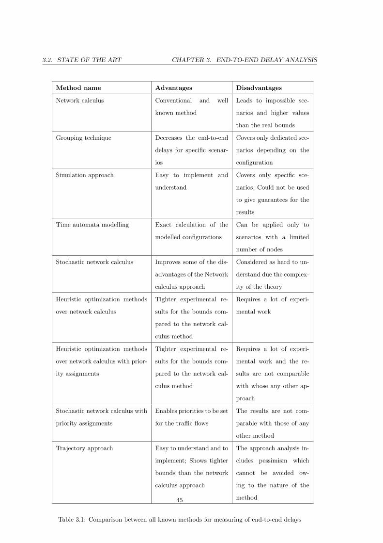
3.2. STATE OF THE ART CHAPTER 3. END-TO-END DELAY ANALYSIS
Method name Advantages Disadvantages
Network calculus Conventional and well
known method
Leads to impossible sce-
narios and higher values
than the real bounds
Grouping technique Decreases the end-to-end
delays for specific scenar-
ios
Covers only dedicated sce-
narios depending on the
configuration
Simulation approach Easy to implement and
understand
Covers only specific sce-
narios; Could not be used
to give guarantees for the
results
Time automata modelling Exact calculation of the
modelled configurations
Can be applied only to
scenarios with a limited
number of nodes
Stochastic network calculus Improves some of the dis-
advantages of the Network
calculus approach
Considered as hard to un-
derstand due the complex-
ity of the theory
Heuristic optimization methods
over network calculus
Tighter experimental re-
sults for the bounds com-
pared to the network cal-
culus method
Requires a lot of experi-
mental work
Heuristic optimization methods
over network calculus with prior-
ity assignments
Tighter experimental re-
sults for the bounds com-
pared to the network cal-
culus method
Requires a lot of experi-
mental work and the re-
sults are not comparable
with whose any other ap-
proach
Stochastic network calculus with
priority assignments
Enables priorities to be set
for the traffic flows
The results are not com-
parable with those of any
other method
Trajectory approach Easy to understand and to
implement; Shows tighter
bounds than the network
calculus approach
The approach analysis in-
cludes pessimism which
cannot be avoided ow-
ing to the nature of the
method
Table 3.1: Comparison between all known methods for measuring of end-to-end delays
45
3.3. ASSUMPTIONS CHAPTER 3. END-TO-END DELAY ANALYSIS
3.3 Assumptions
We have already described the hardware, software configurations and application model
in which we are interested. This has been done in sections 2.2, 2.3 and 2.4. There is
more that has to be considered before we formulate an analysis for the end-to-end delays
of the messages. Firstly we will examine the assumptions for traffic which considers Rate-
Constrained (RC) messages:
� Rate-Constrained (RC) traffic is sporadic. This means that there is no predictability
in the emitting process of the flows. Any time in the period, denoted with Tm for flow
m, could be used as starting time. The constraint is that this should be within the
bounds of the the jitter constraint Jm.
� For the sake of simplicity and further analysis the hardware architecture and the
application model are merged in a manner such that all end systems emit exactly one
virtual link. This is so because the delays produced inside an end system node are
disregarded. This case study excludes processes within the end system.
� The application model and the results of the analysis do not consider any delays due
to a redundancy management system. These modules are not within the scope of the
analysis.
Afterwards the analysis will be extended to include predefined Time-Triggered (TT)
messages. The assumptions related to these were presented in section 2.4. More will be
added if needed.
46
3.4. PRELIMINARY ANALYSIS CHAPTER 3. END-TO-END DELAY ANALYSIS
3.4 Preliminary Analysis
We are interested in the upper bound of the end-to-end delay of Rate-Constrained (RC)
traffic, which represents the maximum waiting service time for emitting, transmitting and
receiving a message, as well as the distribution of this time between its lower and upper
bounds.
By calculating the end-to-end delay of the messages we are aiming:
� to avoid packet loss i.e. none of the switches buffers will overflow
� to limit the end-to-end delay messages to an acceptable time, which is necessary to
maintain the deterministic nature of the AFDX networks
� to prepare the results of the calculations for integration with networks carrying mixed
traffic (Rate-Constrained (RC) and Time-Triggered (TT) messages).
3.4.1 End-to-end delay formula
The first task in our analysis it to build reliable formula that can be used to calculate the
delay if we know the exact constituent parts of it. Let’s consider a virtual link path pm
(the representative of a graph Gm from the configuration). The end-to-end delay Dpm of a
message Fpmis defined as:
Dpm = Tsm + LDFpm+ SDFpm
+WDFpm+ Tr (3.5)
where
� Tsm is the latency of the source end system. This include to the maximum time taken
to obtain application data, tc the maximum time for fragmentation of a message and
ts the maximum time used for polling over the buffers and concatenating the available
frames.
Tsm = to + tc + ts (3.6)
� LDFpmis the transmission delay over the links (between the end system and the switch
or connections between switches). The delay is dependent on the link bandwidth R
47
3.4. PRELIMINARY ANALYSIS CHAPTER 3. END-TO-END DELAY ANALYSIS
(usually 100 Mbit/s). We will denote this delay by L and it will be fixed at 16 µs
multiplied by the number of links (nblpm) in the virtual link path pm
LDFpm= nblpm × L (3.7)
� SDFpmis the transmission delay in the switches for a message Fpm
with length SFpm.
This delay specifically accounts for the time between the input port and the output
port. It is dependant on the size of the messages SFpmand the bandwidth R (usually
100 Mbit/s). As we assume that all devices in a configuration are equal we can
conclude:
SDFpm= nbspm
×(SFpm
/R)
(3.8)
where nbspm is the number of switches in the virtual link path pm.
� WDFpmis the transmission delay in the output port of the switches. This delay is
dependant on the output port load at the moment when the frame/message has to be
transmitted. The delay is
WDFpm=
∑Sk∈nbspm
WDFpm(Sk) (3.9)
where nbspm is the number switches from the path pm and WDFpm(Sk) is the delay
in the output port buffer Sk.
� Tr is the latency of delivery through the destination end system. This delay currently
is considered static.
In conclusion the delay Dpmcan be defined as the sum of the dynamic part (WDFpm
)
and the static part (LDFpm+ SDFpm
).
The results for the cost function Dpm for a frame Fpm transmitted along a virtual link
path pm is are also dependent on these “secondary” factors which have influence on the
dynamic part of Equation 3.9:
� The patterns of message generation (i.e., periodic or sporadic). A given emission might
cause very limited interference with other virtual links messages or the conversely it
might be stacked all the time in the output port of the switches
48
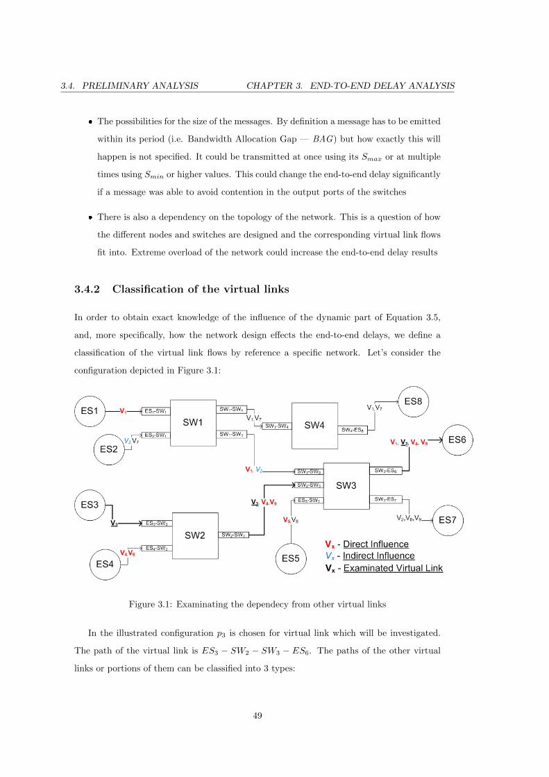
3.4. PRELIMINARY ANALYSIS CHAPTER 3. END-TO-END DELAY ANALYSIS
� The possibilities for the size of the messages. By definition a message has to be emitted
within its period (i.e. Bandwidth Allocation Gap — BAG) but how exactly this will
happen is not specified. It could be transmitted at once using its Smax or at multiple
times using Smin or higher values. This could change the end-to-end delay significantly
if a message was able to avoid contention in the output ports of the switches
� There is also a dependency on the topology of the network. This is a question of how
the different nodes and switches are designed and the corresponding virtual link flows
fit into. Extreme overload of the network could increase the end-to-end delay results
3.4.2 Classification of the virtual links
In order to obtain exact knowledge of the influence of the dynamic part of Equation 3.5,
and, more specifically, how the network design effects the end-to-end delays, we define a
classification of the virtual link flows by reference a specific network. Let’s consider the
configuration depicted in Figure 3.1:
Figure 3.1: Examinating the dependecy from other virtual links
In the illustrated configuration p3 is chosen for virtual link which will be investigated.
The path of the virtual link is ES3 − SW2 − SW3 − ES6. The paths of the other virtual
links or portions of them can be classified into 3 types:
49
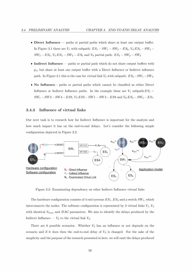
3.4. PRELIMINARY ANALYSIS CHAPTER 3. END-TO-END DELAY ANALYSIS
� Direct Influence — paths or partial paths which share at least one output buffer.
In Figure 3.1 these are V1 with subpath: ES1 − SW1 − SW3 −ES6, V4:ES4 − SW2 −
SW3 − ES6, V5:ES5 − SW3 − ES6 and V9 partial path: ES4 − SW2 − SW3
� Indirect Influence — paths or partial path which do not share output buffers with
pm but share at least one output buffer with a Direct Influence or Indirect influence
path. In Figure 3.1 this is the case for virtual link V2 with subpath: ES2−SW1−SW3.
� No Influence - paths or partial paths which cannot be classified as either Direct
Influence or Indirect Influence paths. In the example these are V1 subpath:ES1 −
SW1−SW2−SW4−ES8, V7:ES2−SW1−SW4−ES8 and V8:ES5−SW3−ES7.
3.4.3 Influence of virtual links
Our next task is to research how far Indirect Influence is important for the analysis and
how much impact it has on the end-to-end delays. Let’s consider the following simple
configuration depicted in Figure 3.2:
Figure 3.2: Examinating dependency on other Indirect Influence virtual links
The hardware configuration consists of 4 end systems ES1..ES4 and a switch SW1, which
interconnects the nodes. The software configuration is represented by 3 virtual links V1..V3
with identical Smax and BAG parameters. We aim to identify the delays produced by the
Indirect Influence — V2 to the virtual link V3.
There are 6 possible scenarios. Whether V2 has an influence or not depends on the
scenario and if it does then the end-to-end delay of V3 is changed. For the sake of the
simplicity and the purpose of the research presented in here, we will omit the delays produced
50
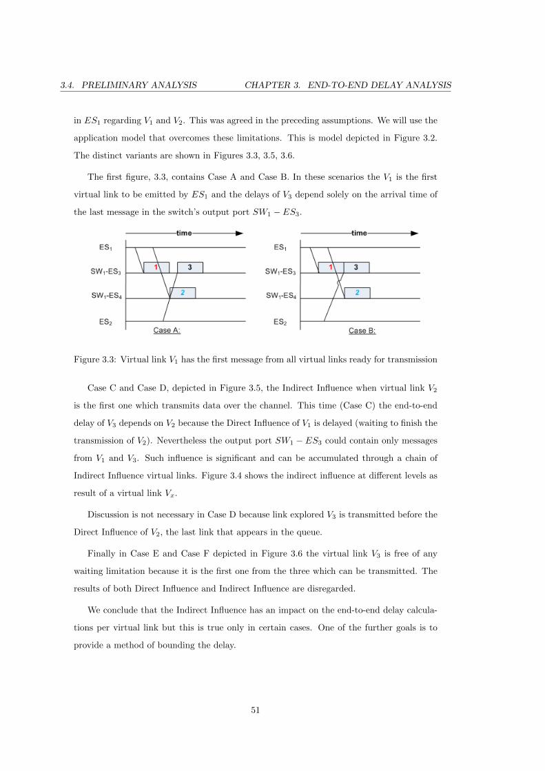
3.4. PRELIMINARY ANALYSIS CHAPTER 3. END-TO-END DELAY ANALYSIS
in ES1 regarding V1 and V2. This was agreed in the preceding assumptions. We will use the
application model that overcomes these limitations. This is model depicted in Figure 3.2.
The distinct variants are shown in Figures 3.3, 3.5, 3.6.
The first figure, 3.3, contains Case A and Case B. In these scenarios the V1 is the first
virtual link to be emitted by ES1 and the delays of V3 depend solely on the arrival time of
the last message in the switch’s output port SW1 − ES3.
Figure 3.3: Virtual link V1 has the first message from all virtual links ready for transmission
Case C and Case D, depicted in Figure 3.5, the Indirect Influence when virtual link V2
is the first one which transmits data over the channel. This time (Case C) the end-to-end
delay of V3 depends on V2 because the Direct Influence of V1 is delayed (waiting to finish the
transmission of V2). Nevertheless the output port SW1 − ES3 could contain only messages
from V1 and V3. Such influence is significant and can be accumulated through a chain of
Indirect Influence virtual links. Figure 3.4 shows the indirect influence at different levels as
result of a virtual link Vx.
Discussion is not necessary in Case D because link explored V3 is transmitted before the
Direct Influence of V2, the last link that appears in the queue.
Finally in Case E and Case F depicted in Figure 3.6 the virtual link V3 is free of any
waiting limitation because it is the first one from the three which can be transmitted. The
results of both Direct Influence and Indirect Influence are disregarded.
We conclude that the Indirect Influence has an impact on the end-to-end delay calcula-
tions per virtual link but this is true only in certain cases. One of the further goals is to
provide a method of bounding the delay.
51
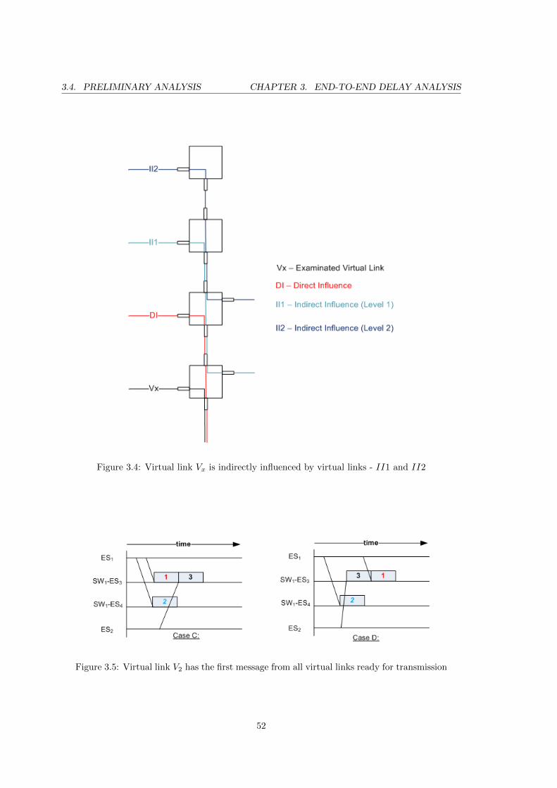
3.4. PRELIMINARY ANALYSIS CHAPTER 3. END-TO-END DELAY ANALYSIS
Figure 3.4: Virtual link Vx is indirectly influenced by virtual links - II1 and II2
Figure 3.5: Virtual link V2 has the first message from all virtual links ready for transmission
52
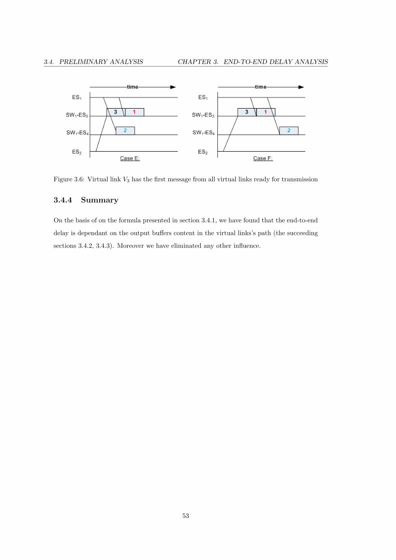
3.4. PRELIMINARY ANALYSIS CHAPTER 3. END-TO-END DELAY ANALYSIS
Figure 3.6: Virtual link V3 has the first message from all virtual links ready for transmission
3.4.4 Summary
On the basis of on the formula presented in section 3.4.1, we have found that the end-to-end
delay is dependant on the output buffers content in the virtual links’s path (the succeeding
sections 3.4.2, 3.4.3). Moreover we have eliminated any other influence.
53
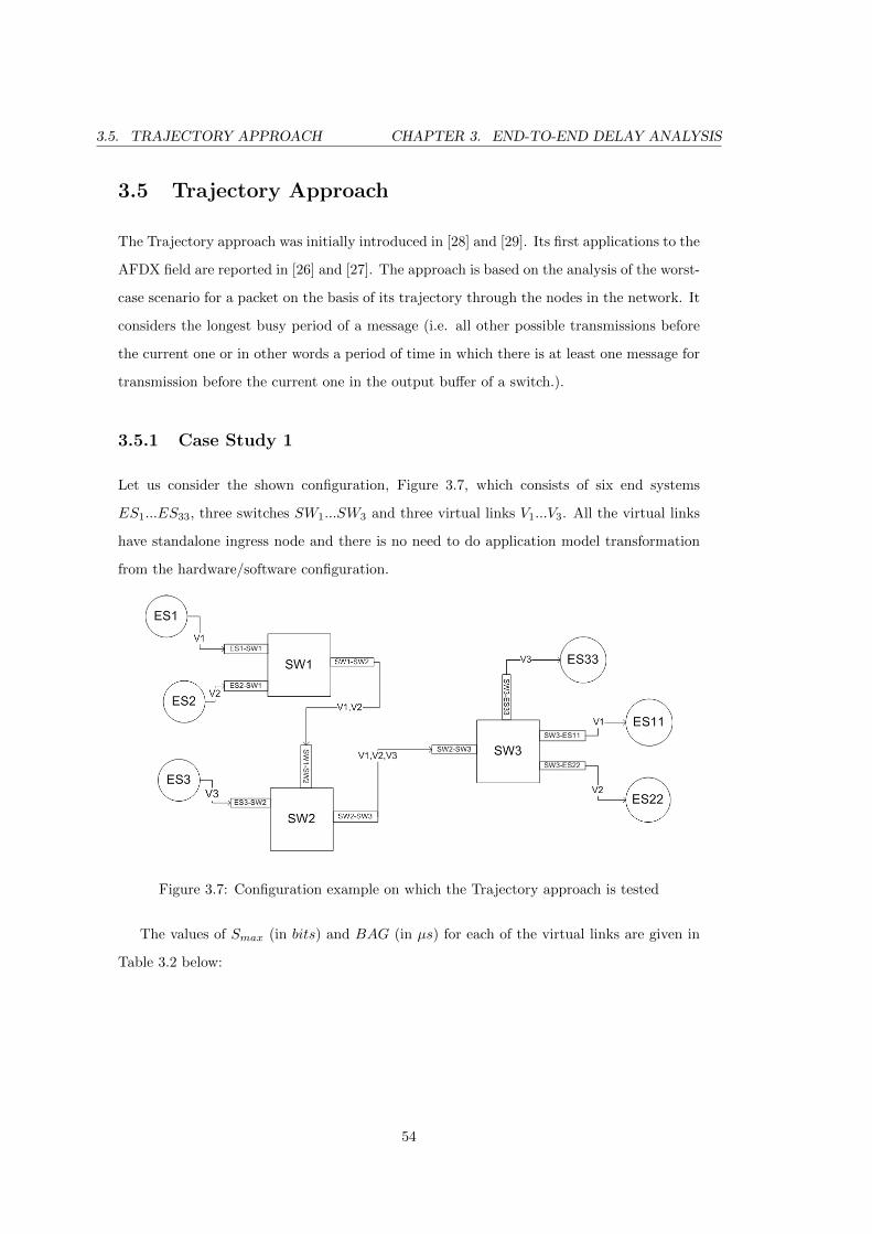
3.5. TRAJECTORY APPROACH CHAPTER 3. END-TO-END DELAY ANALYSIS
3.5 Trajectory Approach
The Trajectory approach was initially introduced in [28] and [29]. Its first applications to the
AFDX field are reported in [26] and [27]. The approach is based on the analysis of the worst-
case scenario for a packet on the basis of its trajectory through the nodes in the network. It
considers the longest busy period of a message (i.e. all other possible transmissions before
the current one or in other words a period of time in which there is at least one message for
transmission before the current one in the output buffer of a switch.).
3.5.1 Case Study 1
Let us consider the shown configuration, Figure 3.7, which consists of six end systems
ES1...ES33, three switches SW1...SW3 and three virtual links V1...V3. All the virtual links
have standalone ingress node and there is no need to do application model transformation
from the hardware/software configuration.
Figure 3.7: Configuration example on which the Trajectory approach is tested
The values of Smax (in bits) and BAG (in µs) for each of the virtual links are given in
Table 3.2 below:
54
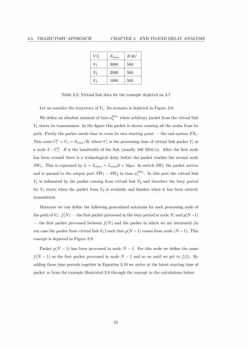
3.5. TRAJECTORY APPROACH CHAPTER 3. END-TO-END DELAY ANALYSIS
V L Smax BAG
V1 3000 500
V2 2000 500
V3 1000 500
Table 3.2: Virtual link data for the example depicted on 3.7
Let us consider the trajectory of V1. Its scenario is depicted in Figure 3.8:
We define an absolute moment of time aES13 where arbitrary packet from the virtual link
V1 starts its transmission. In the figure this packet is shown crossing all the nodes from its
path. Firstly the packet needs time to cross its own starting point — the end system ES1.
This costs Chi = Ci = Smax/R, where Ci is the processing time of virtual link packet Vi in
a node h - Chi . R is the bandwidth of the link (usually 100 Mbit/s). After the first node
has been crossed there is a technological delay before the packet reaches the second node
SW1. This is expressed by L = Lmin = Lmax0 = 16µs. In switch SW1 the packet arrives
and is queued to the output port SW1 − SW2 in time aSW11 . In this port the virtual link
V1 is influenced by the packet coming from virtual link V2 and therefore the busy period
for V1 starts when the packet from V2 is available and finishes when it has been entirely
transmitted.
Moreover we can define the following generalized notations for each processing node of
the path of V1: f(N) — the first packet processed in the busy period in node N ; and p(N−1)
— the first packet processed between f(N) and the packet in which we are interested (in
our case the packet from virtual link V1) such that p(N − 1) comes from node (N − 1). This
concept is depicted in Figure 3.9:
Packet p(N − 1) has been processed in node N − 1. For this node we define the same
f(N − 1) as the first packet processed in node N − 1 and so on until we get to f(1). By
adding these time periods together in Equation 3.10 we arrive at the latest starting time of
packet m from the example illustrated 3.9 through the concept in the calculations below:
55
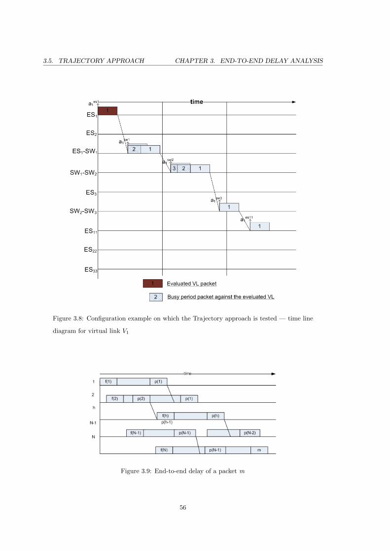
3.5. TRAJECTORY APPROACH CHAPTER 3. END-TO-END DELAY ANALYSIS
Figure 3.8: Configuration example on which the Trajectory approach is tested — time line
diagram for virtual link V1
Figure 3.9: End-to-end delay of a packet m
56
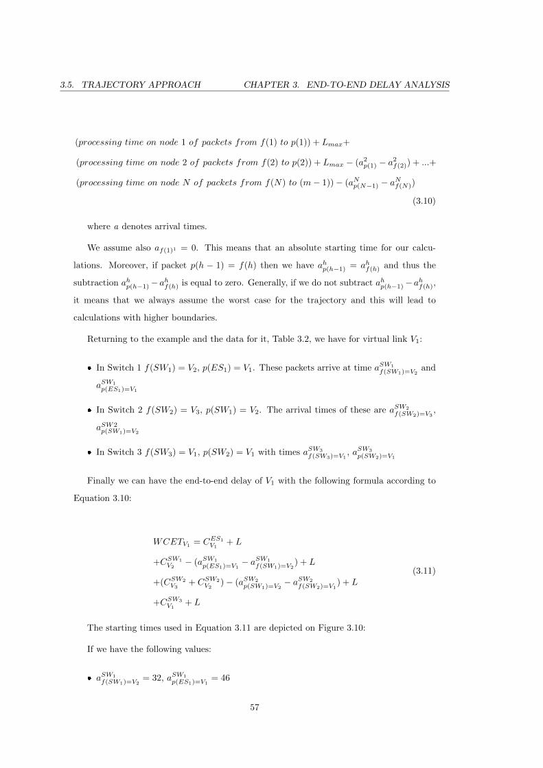
3.5. TRAJECTORY APPROACH CHAPTER 3. END-TO-END DELAY ANALYSIS
(processing time on node 1 of packets from f(1) to p(1)) + Lmax+
(processing time on node 2 of packets from f(2) to p(2)) + Lmax − (a2p(1) − a
2f(2)) + ...+
(processing time on node N of packets from f(N) to (m− 1))− (aNp(N−1) − aNf(N))
(3.10)
where a denotes arrival times.
We assume also af(1)1 = 0. This means that an absolute starting time for our calcu-
lations. Moreover, if packet p(h − 1) = f(h) then we have ahp(h−1) = ahf(h) and thus the
subtraction ahp(h−1)−ahf(h) is equal to zero. Generally, if we do not subtract ahp(h−1)−a
hf(h),
it means that we always assume the worst case for the trajectory and this will lead to
calculations with higher boundaries.
Returning to the example and the data for it, Table 3.2, we have for virtual link V1:
� In Switch 1 f(SW1) = V2, p(ES1) = V1. These packets arrive at time aSW1
f(SW1)=V2and
aSW1
p(ES1)=V1
� In Switch 2 f(SW2) = V3, p(SW1) = V2. The arrival times of these are aSW2
f(SW2)=V3,
aSW2p(SW1)=V2
� In Switch 3 f(SW3) = V1, p(SW2) = V1 with times aSW3
f(SW3)=V1, aSW3
p(SW2)=V1
Finally we can have the end-to-end delay of V1 with the following formula according to
Equation 3.10:
WCETV1= CES1
V1+ L
+CSW1
V2− (aSW1
p(ES1)=V1− aSW1
f(SW1)=V2) + L
+(CSW2
V3+ CSW2
V2)− (aSW2
p(SW1)=V2− aSW2
f(SW2)=V1) + L
+CSW3
V1+ L
(3.11)
The starting times used in Equation 3.11 are depicted on Figure 3.10:
If we have the following values:
� aSW1
f(SW1)=V2= 32, aSW1
p(ES1)=V1= 46
57
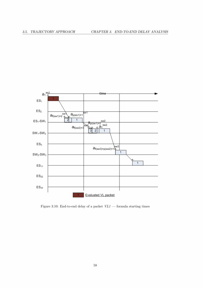
3.5. TRAJECTORY APPROACH CHAPTER 3. END-TO-END DELAY ANALYSIS
Figure 3.10: End-to-end delay of a packet VL1 — formula starting times
58
3.5. TRAJECTORY APPROACH CHAPTER 3. END-TO-END DELAY ANALYSIS
� aSW2
f(SW2)=V3= 85, aSW2
p(SW1)=V2= 102, aSW2
1 = 115
� aSW3
f(SW3)=V1= 155, aSW3
p(SW2)=V1= 155
and we calculate with Equation 3.11, then as final result for the WCET of packet of virtual
link V1 we have:
WCETV1 = 30+16+20−(46−32)+16+(20+10)−(102−85)+16+30+16 = 143 (3.12)
where C is calculated as C = Smax/R according the virtual link.
59
3.6. COMPUTATIONS CHAPTER 3. END-TO-END DELAY ANALYSIS
3.6 Computations
The Trajectory approach result is computed in [28]. In this section we summarize the results
and give the necessary formula for the computations.
The worst case end-to-end response time of any packet from virtual link i is bounded by:
Ri = maxt≥−Ji
(W lastii,t + Clasti
i − t) (3.13)
where lasti is the last node visited in the path Pi and W lastii,t is the latest starting time
of a packet generated at time t at the last node it visited. More specifically W lastii,t is
W lastii,t =
∑j∈[1,n];j 6=i;Pi∩Pj 6=∅
(1 + b t+Ai,j
Tjc)+
× Cj +
(1 + b t+ Ji
Tic)× Ci
+∑
h∈Pi;h 6=lasti
(max
j∈[1,n];h∈Pj
{Cj})− Ci + |Pi + 1|.Lmax (3.14)
where
� (x+) = max {0, x}
�
∑j∈[1,n];j 6=i;Pi∩Pj 6=∅
(1 + b t+Ai,j
Tjc)+
× Cj is the processing time of the packets from
flows crossing the flow being investigated - virtual link Vi. The analysis in [28] shows
that this time has to be considered in the slowest node, but apparently all switches in
the AFDX network are equal. Ai,j is the maximum jitter of any flow intersecting Vi
� Ai,j = min(Sfirstj,imaxi = W
lasti,ji,t − Sfirstj,i
minj; t)−Mfirsti,j
i + Sfirsti,jmaxj + Jj
� Mhi =
∑prei(h)
h=firsti(minj∈[1,n];firstj,i=firsti,j {Cj}+ Lmin)
� Shmin is the minimum time taken by a packet of Vi to go from its source node to node
denoted by h
� Shmax is the maximum time taken by a packet of Vi to go from its source node to node
denoted by h
�
(1 + b t+Ji
Tic)× Ci is the processing time of virtual link Vi on the slowest node on its
path
60
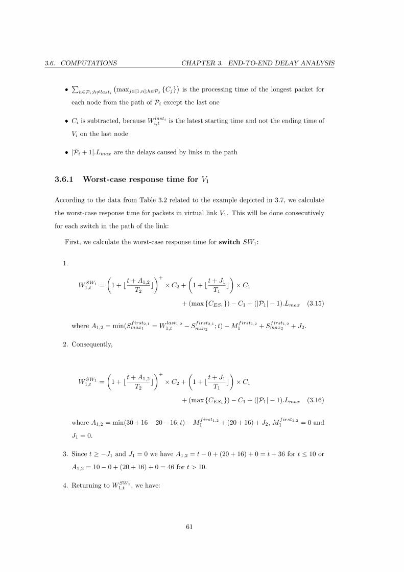
3.6. COMPUTATIONS CHAPTER 3. END-TO-END DELAY ANALYSIS
�
∑h∈Pi;h6=lasti
(maxj∈[1,n];h∈Pj
{Cj})
is the processing time of the longest packet for
each node from the path of Pi except the last one
� Ci is subtracted, because W lastii,t is the latest starting time and not the ending time of
Vi on the last node
� |Pi + 1|.Lmax are the delays caused by links in the path
3.6.1 Worst-case response time for V1
According to the data from Table 3.2 related to the example depicted in 3.7, we calculate
the worst-case response time for packets in virtual link V1. This will be done consecutively
for each switch in the path of the link:
First, we calculate the worst-case response time for switch SW1:
1.
WSW11,t =
(1 + b t+A1,2
T2c)+
× C2 +
(1 + b t+ J1
T1c)× C1
+ (max {CES1})− C1 + (|P1| − 1).Lmax (3.15)
where A1,2 = min(Sfirst2,1max1 = W
last1,21,t − Sfirst2,1
min2; t)−Mfirst1,2
1 + Sfirst1,2max2 + J2.
2. Consequently,
WSW11,t =
(1 + b t+A1,2
T2c)+
× C2 +
(1 + b t+ J1
T1c)× C1
+ (max {CES1})− C1 + (|P1| − 1).Lmax (3.16)
where A1,2 = min(30 + 16− 20− 16; t)−Mfirst1,21 + (20 + 16) + J2, M
first1,21 = 0 and
J1 = 0.
3. Since t ≥ −J1 and J1 = 0 we have A1,2 = t− 0 + (20 + 16) + 0 = t+ 36 for t ≤ 10 or
A1,2 = 10− 0 + (20 + 16) + 0 = 46 for t > 10.
4. Returning to WSW11,t , we have:
61
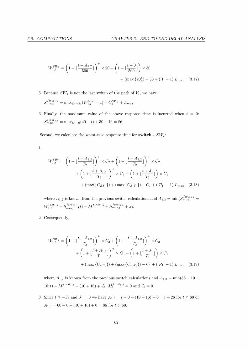
3.6. COMPUTATIONS CHAPTER 3. END-TO-END DELAY ANALYSIS
WSW11,t =
(1 + b t+A1,2
500c)+
× 20 +
(1 + b t+ 0
500c)× 30
+ (max {20})− 30 + (|1| − 1).Lmax (3.17)
5. Because SW1 is not the last switch of the path of V1, we have
Sfirst2,1max1 = maxt≥−J1(WSW1
1,t − t) + CSW11 + Lmax
6. Finally, the maximum value of the above response time is incurred when t = 0:
Sfirst2,1max1 = maxt≥−0(40− t) + 30 + 16 = 86.
Second, we calculate the worst-case response time for switch - SW2:
1.
WSW21,t =
(1 + b t+A1,2
T2c)+
× C2 +
(1 + b t+A1,2
T2c)+
× C2
+
(1 + b t+A1,3
T3c)+
× C3 +
(1 + b t+ J1
T1c)× C1
+ (max {CES1}) + (max {CSW1
})− C1 + (|P1| − 1).Lmax (3.18)
where A1,2 is known from the previous switch calculations and A1,3 = min(Sfirst3,1max1 =
Wlast1,31,t − Sfirst3,1
min3; t)−Mfirst1,3
1 + Sfirst1,3max3 + J3.
2. Consequently,
WSW21,t =
(1 + b t+A1,2
T2c)+
× C2 +
(1 + b t+A1,2
T2c)+
× C2
+
(1 + b t+A1,3
T3c)+
× C3 +
(1 + b t+ J1
T1c)× C1
+ (max {CES1}) + (max {CSW1})− C1 + (|P1| − 1).Lmax (3.19)
where A1,2 is known from the previous switch calculations and A1,3 = min(86− 10−
16; t)−Mfirst1,31 + (10 + 16) + J3, M
first1,31 = 0 and J3 = 0.
3. Since t ≥ −J1 and J1 = 0 we have A1,3 = t+ 0 + (10 + 16) + 0 = t+ 26 for t ≤ 60 or
A1,3 = 60 + 0 + (10 + 16) + 0 = 86 for t > 60.
62
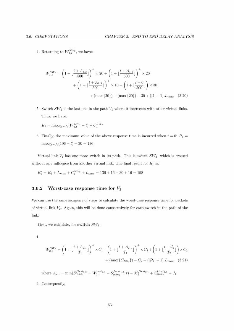
3.6. COMPUTATIONS CHAPTER 3. END-TO-END DELAY ANALYSIS
4. Returning to WSW21,t , we have:
WSW21,t =
(1 + b t+A1,2
500c)+
× 20 +
(1 + b t+A1,2
500c)+
× 20
+
(1 + b t+A1,3
500c)+
× 10 +
(1 + b t+ 0
500c)× 30
+ (max {20}) + (max {20})− 30 + (|2| − 1).Lmax (3.20)
5. Switch SW2 is the last one in the path V1 where it intersects with other virtual links.
Thus, we have:
R1 = maxt≥−J1(WSW2
1,t − t) + CSW21
6. Finally, the maximum value of the above response time is incurred when t = 0: R1 =
maxt≥−J1(106− t) + 30 = 136
Virtual link V1 has one more switch in its path. This is switch SW3, which is crossed
without any influence from another virtual link. The final result for R1 is:
R∗1 = R1 + Lmax + CSW31 + Lmax = 136 + 16 + 30 + 16 = 198
3.6.2 Worst-case response time for V2
We can use the same sequence of steps to calculate the worst-case response time for packets
of virtual link V2. Again, this will be done consecutively for each switch in the path of the
link:
First, we calculate, for switch SW1:
1.
WSW12,t =
(1 + b t+A2,1
T1c)+
×C1 +
(1 + b t+A2,1
T1c)+
×C1 +
(1 + b t+ J2
T2c)×C2
+ (max {CES2})− C2 + (|P2| − 1).Lmax (3.21)
where A2,1 = min(Sfirst1,2max2 = W
last2,12,t − Sfirst1,2
min1; t)−Mfirst2,1
2 + Sfirst2,1max1 + J1.
2. Consequently,
63
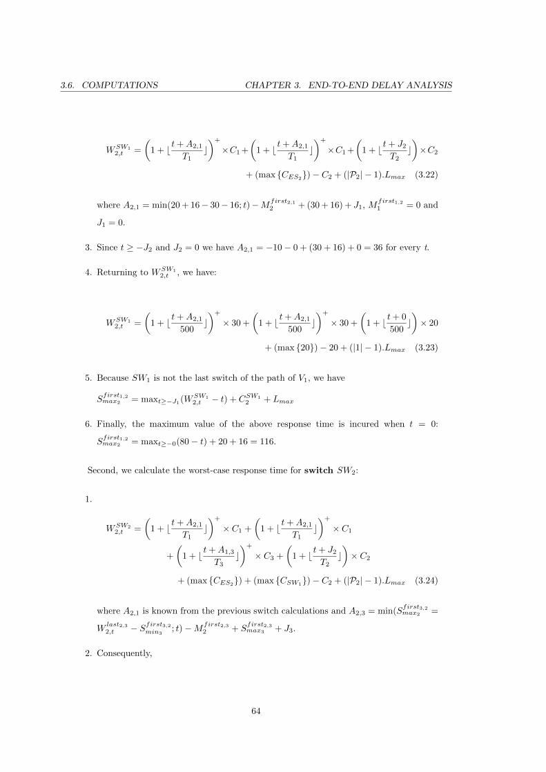
3.6. COMPUTATIONS CHAPTER 3. END-TO-END DELAY ANALYSIS
WSW12,t =
(1 + b t+A2,1
T1c)+
×C1 +
(1 + b t+A2,1
T1c)+
×C1 +
(1 + b t+ J2
T2c)×C2
+ (max {CES2})− C2 + (|P2| − 1).Lmax (3.22)
where A2,1 = min(20 + 16− 30− 16; t)−Mfirst2,12 + (30 + 16) + J1, M
first1,21 = 0 and
J1 = 0.
3. Since t ≥ −J2 and J2 = 0 we have A2,1 = −10− 0 + (30 + 16) + 0 = 36 for every t.
4. Returning to WSW12,t , we have:
WSW12,t =
(1 + b t+A2,1
500c)+
× 30 +
(1 + b t+A2,1
500c)+
× 30 +
(1 + b t+ 0
500c)× 20
+ (max {20})− 20 + (|1| − 1).Lmax (3.23)
5. Because SW1 is not the last switch of the path of V1, we have
Sfirst1,2max2 = maxt≥−J1(WSW1
2,t − t) + CSW12 + Lmax
6. Finally, the maximum value of the above response time is incured when t = 0:
Sfirst1,2max2 = maxt≥−0(80− t) + 20 + 16 = 116.
Second, we calculate the worst-case response time for switch SW2:
1.
WSW22,t =
(1 + b t+A2,1
T1c)+
× C1 +
(1 + b t+A2,1
T1c)+
× C1
+
(1 + b t+A1,3
T3c)+
× C3 +
(1 + b t+ J2
T2c)× C2
+ (max {CES2}) + (max {CSW1
})− C2 + (|P2| − 1).Lmax (3.24)
where A2,1 is known from the previous switch calculations and A2,3 = min(Sfirst3,2max2 =
Wlast2,32,t − Sfirst3,2
min3; t)−Mfirst2,3
2 + Sfirst2,3max3 + J3.
2. Consequently,
64
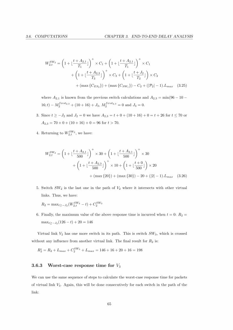
3.6. COMPUTATIONS CHAPTER 3. END-TO-END DELAY ANALYSIS
WSW22,t =
(1 + b t+A2,1
T1c)+
× C1 +
(1 + b t+A2,1
T1c)+
× C1
+
(1 + b t+A2,3
T3c)+
× C3 +
(1 + b t+ J2
T2c)× C2
+ (max {CES2}) + (max {CSW1
})− C2 + (|P2| − 1).Lmax (3.25)
where A2,1 is known from the previous switch calculations and A2,3 = min(96− 10−
16; t)−Mfirst2,32 + (10 + 16) + J3, M
first2,32 = 0 and J3 = 0.
3. Since t ≥ −J2 and J2 = 0 we have A2,3 = t+ 0 + (10 + 16) + 0 = t+ 26 for t ≤ 70 or
A2,3 = 70 + 0 + (10 + 16) + 0 = 96 for t > 70.
4. Returning to WSW22,t , we have:
WSW22,t =
(1 + b t+A2,1
500c)+
× 30 +
(1 + b t+A2,1
500c)+
× 30
+
(1 + b t+A2,3
500c)+
× 10 +
(1 + b t+ 0
500c)× 20
+ (max {20}) + (max {30})− 20 + (|2| − 1).Lmax (3.26)
5. Switch SW2 is the last one in the path of V2 where it intersects with other virtual
links. Thus, we have:
R2 = maxt≥−J2(WSW2
2,t − t) + CSW22
6. Finally, the maximum value of the above response time is incurred when t = 0: R2 =
maxt≥−J2(126− t) + 20 = 146
Virtual link V2 has one more switch in its path. This is switch SW3, which is crossed
without any influence from another virtual link. The final result for R2 is:
R∗2 = R2 + Lmax + CSW32 + Lmax = 146 + 16 + 20 + 16 = 198
3.6.3 Worst-case response time for V3
We can use the same sequence of steps to calculate the worst-case response time for packets
of virtual link V3. Again, this will be done consecutively for each switch in the path of the
link:
65
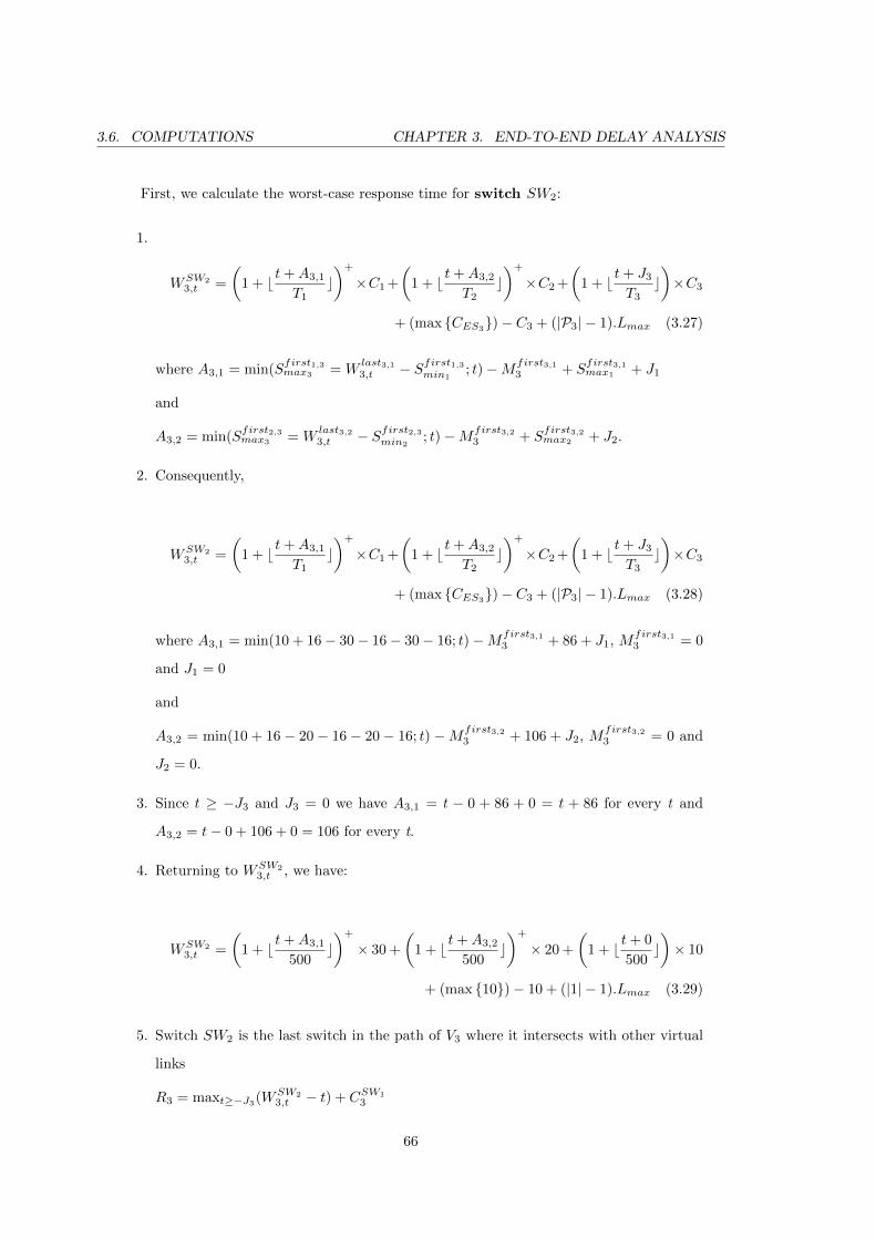
3.6. COMPUTATIONS CHAPTER 3. END-TO-END DELAY ANALYSIS
First, we calculate the worst-case response time for switch SW2:
1.
WSW23,t =
(1 + b t+A3,1
T1c)+
×C1 +
(1 + b t+A3,2
T2c)+
×C2 +
(1 + b t+ J3
T3c)×C3
+ (max {CES3})− C3 + (|P3| − 1).Lmax (3.27)
where A3,1 = min(Sfirst1,3max3 = W
last3,13,t − Sfirst1,3
min1; t)−Mfirst3,1
3 + Sfirst3,1max1 + J1
and
A3,2 = min(Sfirst2,3max3 = W
last3,23,t − Sfirst2,3
min2; t)−Mfirst3,2
3 + Sfirst3,2max2 + J2.
2. Consequently,
WSW23,t =
(1 + b t+A3,1
T1c)+
×C1 +
(1 + b t+A3,2
T2c)+
×C2 +
(1 + b t+ J3
T3c)×C3
+ (max {CES3})− C3 + (|P3| − 1).Lmax (3.28)
where A3,1 = min(10 + 16− 30− 16− 30− 16; t)−Mfirst3,13 + 86 + J1, M
first3,13 = 0
and J1 = 0
and
A3,2 = min(10 + 16 − 20 − 16 − 20 − 16; t) −Mfirst3,23 + 106 + J2, M
first3,23 = 0 and
J2 = 0.
3. Since t ≥ −J3 and J3 = 0 we have A3,1 = t − 0 + 86 + 0 = t + 86 for every t and
A3,2 = t− 0 + 106 + 0 = 106 for every t.
4. Returning to WSW23,t , we have:
WSW23,t =
(1 + b t+A3,1
500c)+
× 30 +
(1 + b t+A3,2
500c)+
× 20 +
(1 + b t+ 0
500c)× 10
+ (max {10})− 10 + (|1| − 1).Lmax (3.29)
5. Switch SW2 is the last switch in the path of V3 where it intersects with other virtual
links
R3 = maxt≥−J3(WSW23,t − t) + CSW1
3
66

3.6. COMPUTATIONS CHAPTER 3. END-TO-END DELAY ANALYSIS
6. Finally, the maximum value of the above response time is incurred when t = 0: R3 =
maxt≥−0(60− t) + 10 = 70
Virtual link V3 has one more switch in its path. This is switch SW3, which is crossed
without any influence from another virtual link. The final result for R3 is:
R∗3 = R3 + Lmax + CSW33 + Lmax = 70 + 16 + 10 + 16 = 112
67
Chapter 4
(II) and (TT) messages
4.1 Introduction
In this chapter we investigate two important aspects of AFDX networks and the models
covered so far.
The first one is related to the Indirect Influence (II) of the virtual links. This influence is
introduced in section 3.4, but there is no example yet of how it is integrated in the Trajectory
approach.
The second feature which is discussed in this chapter is related to the integration of
Rate-Constrained (RC) messages with Time-Triggered (TT) ones. Again, this is done by
modifying the formula for the Trajectory approach and using a special case of it.
68
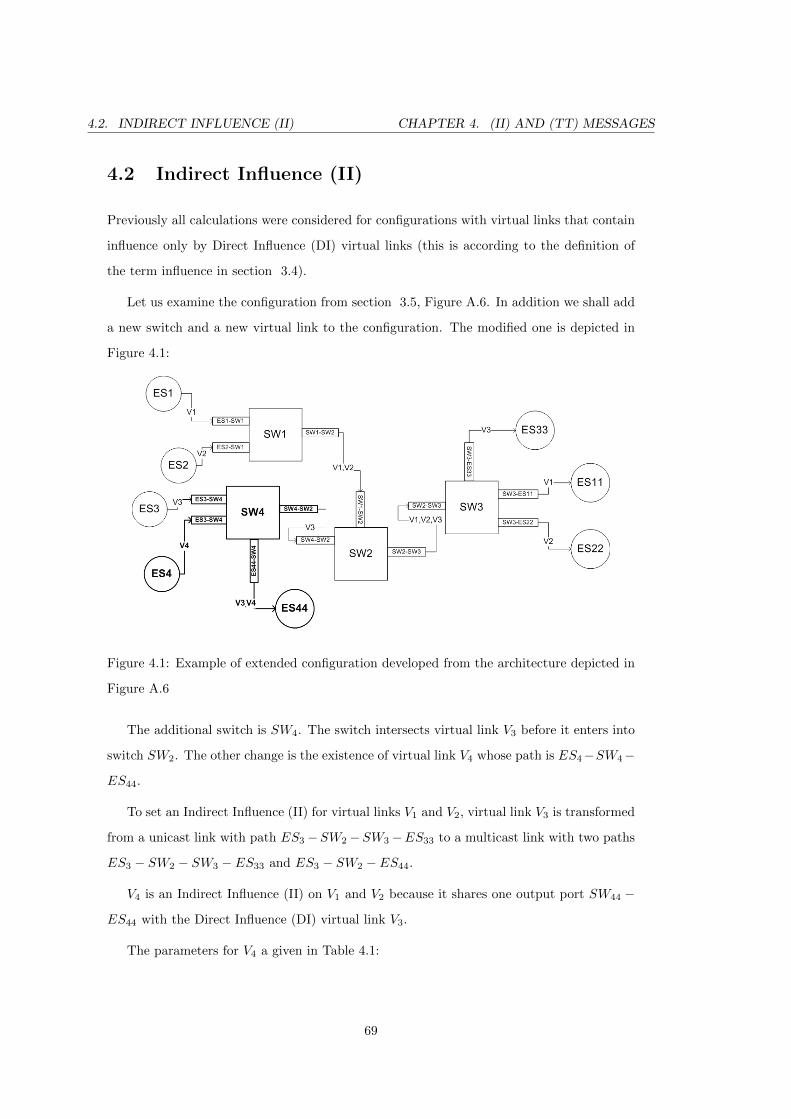
4.2. INDIRECT INFLUENCE (II) CHAPTER 4. (II) AND (TT) MESSAGES
4.2 Indirect Influence (II)
Previously all calculations were considered for configurations with virtual links that contain
influence only by Direct Influence (DI) virtual links (this is according to the definition of
the term influence in section 3.4).
Let us examine the configuration from section 3.5, Figure A.6. In addition we shall add
a new switch and a new virtual link to the configuration. The modified one is depicted in
Figure 4.1:
Figure 4.1: Example of extended configuration developed from the architecture depicted in
Figure A.6
The additional switch is SW4. The switch intersects virtual link V3 before it enters into
switch SW2. The other change is the existence of virtual link V4 whose path is ES4−SW4−
ES44.
To set an Indirect Influence (II) for virtual links V1 and V2, virtual link V3 is transformed
from a unicast link with path ES3−SW2−SW3−ES33 to a multicast link with two paths
ES3 − SW2 − SW3 − ES33 and ES3 − SW2 − ES44.
V4 is an Indirect Influence (II) on V1 and V2 because it shares one output port SW44 −
ES44 with the Direct Influence (DI) virtual link V3.
The parameters for V4 a given in Table 4.1:
69
4.2. INDIRECT INFLUENCE (II) CHAPTER 4. (II) AND (TT) MESSAGES
V L Smax BAG
V4 1500 500
Table 4.1: Virtual link V4 parameters
On the basis of the Trajectory approach formula, we will rebuild the calculations of the
worst-case response time of the virtual links. Obviously, the delay of virtual link V3 will be
increased by at least CSWV3
+ Lmax. Moreover, we recalculate the delay of V3:
First, we calculate the worst-case response time for switch SW4 — the new first switch
in the virtual links path:
1.
WSW43,t =
(1 + b t+A3,4
T4c)+
× C4 +
(1 + b t+ J3
T3c)× C3
+ (max {CES3})− C3 + (|P3| − 1).Lmax (4.1)
where A3,4 = min(Sfirst4,3max3 = W
last3,43,t − Sfirst4,3
min4; t)−Mfirst3,4
3 + Sfirst3,4max4 + J4 .
2. Consequently,
WSW43,t =
(1 + b t+A3,4
T4c)+
× C4 +
(1 + b t+ J3
T3c)× C3
+ (max {CES3})− C3 + (|P3| − 1).Lmax (4.2)
where A3,4 = min(10 + 16− 15− 16; t)−Mfirst3,43 + 0 + J1, M
first3,13 = 0 and J1 = 0.
3. Since t ≥ −J3 and J3 = 0 we have A3,4 = t− 0 + 0 + 0 = t+ t for every t.
4. Returning to WSW43,t , we have:
WSW43,t =
(1 + b t+A3,4
500c)+
× 15 +
(1 + b t+ 0
500c)× 10
+ (max {10})− 10 + (|1| − 1).Lmax (4.3)
5. Switch SW2 is the last switch in the path of V3 where it intersects with other virtual
links
R3 = maxt≥−J3(WSW23,t − t) + CSW1
3
70
4.2. INDIRECT INFLUENCE (II) CHAPTER 4. (II) AND (TT) MESSAGES
6. Finally, the maximum value of the above response time is incurred when t = 0: R3 =
maxt≥−0(25− t) + 10 = 35
Virtual link V3 has one more switch (SW2) in its path, namely which intersects with
other virtual links V1 and V2.
We will calculate the worst-case response time for switch SW2:
1.
WSW23,t =
(1 + b t+A3,4
T4c)+
× C4 +
(1 + b t+A3,1
T1c)+
× C1
+
(1 + b t+A3,2
T2c)+
× C2 +
(1 + b t+ J3
T3c)× C3
+ (max {CES3}) + (max {CSW4
})− C3 + (|P3| − 1).Lmax (4.4)
where A3,1 is known from previous calculations, A3,1 = min(Sfirst1,3max3 = W
last3,13,t −
Sfirst1,3min1
; t)−Mfirst3,13 + S
first3,1max1 + J1
and
A3,2 = min(Sfirst2,3max3 = W
last3,23,t − Sfirst2,3
min2; t)−Mfirst3,2
3 + Sfirst3,2max2 + J2.
2. Consequently,
WSW23,t =
(1 + b t+A3,4
T4c)+
× C4 +
(1 + b t+A3,1
T1c)+
× C1
+
(1 + b t+A3,2
T2c)+
× C2 +
(1 + b t+ J3
T3c)× C3
+ (max {CES3}) + (max {CSW4
})− C3 + (|P3| − 1).Lmax (4.5)
where A3,1 = min(10 + 16− 30− 16− 30− 16; t)−Mfirst3,13 + 86 + J1, M
first3,13 = 0
and J1 = 0
and
A3,2 = min(10 + 16 − 20 − 16 − 20 − 16; t) −Mfirst3,23 + 106 + J2, M
first3,23 = 0 and
J2 = 0.
3. Since t ≥ −J3 and J3 = 0 we have A3,1 = t − 0 + 86 + 0 = t + 86 for every t and
A3,2 = t− 0 + 106 + 0 = 106 for every t.
71
4.2. INDIRECT INFLUENCE (II) CHAPTER 4. (II) AND (TT) MESSAGES
4. Returning to WSW23,t , we have:
WSW23,t =
(1 + b t+A3,4
500c)+
× 15 +
(1 + b t+A3,1
500c)+
× 30
+
(1 + b t+A3,2
500c)+
× 20 +
(1 + b t+ 0
500c)× 10
+ (max {10}) + (max {15})− 10 + (|2| − 1).Lmax (4.6)
5. Switch SW2 is the last switch in the path of V3 where it intersects with other virtual
links
R3 = maxt≥−J3(WSW2
3,t − t) + CSW23
6. Finally, the maximum value of the above response time is incurred when t = 0: R3 =
maxt≥−0(90− t) + 10 = 100
Virtual link V3 has one more switch in its path. This is switch SW3, which is crossed
without any influence from another virtual link. The final result for R3 is:
R∗3 = R3 + Lmax + CSW33 + Lmax = 100 + 16 + 10 + 16 = 142
We showed in the above calculations that the worst-case response time is changed in
terms of the added additional time needed for processing V3 packets.
If we apply new calculations for V1 and V2 the results will be changed for A1,3 and A2,3
in the respective formulas. Therefore, we will not investigate further the Indirect Influence
(II) of the virtual links in this category. We accept that this influence is irrelevant for
the Trajectory approach. This is so because of the asynchronous nature of the network end
nodes. If a message from virtual link V3 is delayed owing to V4 (the Indirect Influence (II) for
V1 and V2), then the possible influence resulting from this delay is equal to the asynchronous
behaviour of the arrival time in SW2.
72
4.3. TIME-TRIGGERED (TT) MESSAGES CHAPTER 4. (II) AND (TT) MESSAGES
4.3 Time-Triggered (TT) messages
We have skipped the Indirect Influence (II) virtual links in the example configuration de-
picted in Figure A.6. They were introduced in the previous section 4.2. We will do the
same for the Time-Triggered (TT) messages which will exist next to the Rate-Constrained
(RC) messages. The properties of the Time-Triggered (TT) messages are given in section
1.3.1. By their nature these messages are traffic which has predefined timeslots and takes
precedence over any other traffic. Therefore we will not calculate the worst-case response
time of it. Our goal is to estimate the influence by the Time-Triggered (TT) traffic over the
Rate-Constrained (RC) traffic.
We use the original Trajectory approach document [29] which presents several cases of
the method. One of them is related to FP/FIFO∗13 scheduling. This alternative is a
method that is similar to the scheduling produced from Time-Triggered (TT) traffic and
Rate-Constrained (RC) traffic for TTEthernet networks. From now on we will assume
that all examples that combine Rate-Constrained (RC) messages and Time-Triggered (TT)
messages are configurations compatible with the described in 2.2, 2.3 and 2.4 but with
Time-Triggered (TT) capabilities (as the ones presented in section 1.3).
Let us consider the configuration from section 3.5, Figure A.6, which consists from six
end systems ES1...ES33, three switches SW1...SW3 and three virtual links V1...V3. All
virtual links have standalone ingress nodes and it is not required to do an application
model transformation of the hardware/software configuration. Additionally V3 emits no
more Rate-Constrained (RC) messages. They are replaced by Time-Triggered (TT) mes-
sages. Illustratively this is depicted in Figure A.7. SW2 can handle both types of traffic
(Rate-Constrained (RC) and Time-Triggered (TT))and the end nodes ES3, ES33 have the
same capabilities.
We assume that the virtual link V3 has the same values for the BAG and Smax properties
as previously when it was dedicated only for Rate-Constrained (RC) traffic. On the basis
of the Trajectory approach formula and special case of it, we redo the calculations of the
worst-case response time of virtual links V1 and V2. Obviously virtual link V3 worst-case
response time will not be changed because the link has guarantees provided from its traffic
class. It is expected that the worst-case response time of links V1 and V2 will be increased.
13Fixed Priority / First In, First Out
73
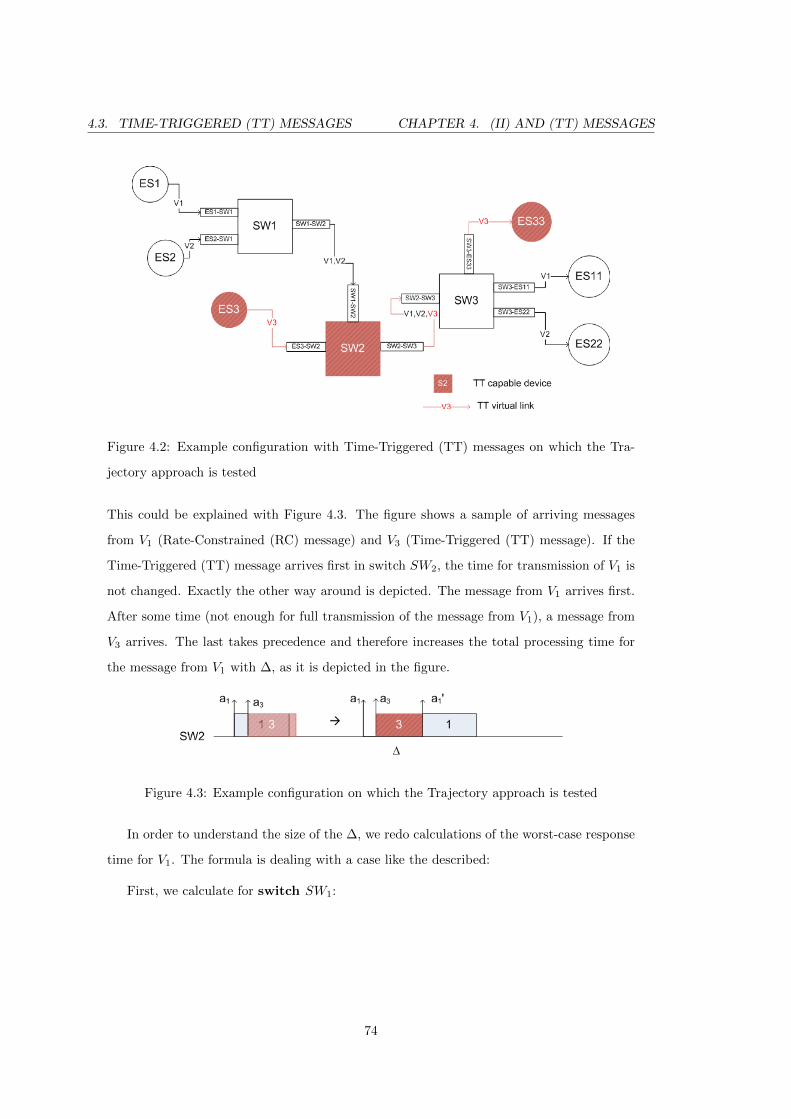
4.3. TIME-TRIGGERED (TT) MESSAGES CHAPTER 4. (II) AND (TT) MESSAGES
Figure 4.2: Example configuration with Time-Triggered (TT) messages on which the Tra-
jectory approach is tested
This could be explained with Figure 4.3. The figure shows a sample of arriving messages
from V1 (Rate-Constrained (RC) message) and V3 (Time-Triggered (TT) message). If the
Time-Triggered (TT) message arrives first in switch SW2, the time for transmission of V1 is
not changed. Exactly the other way around is depicted. The message from V1 arrives first.
After some time (not enough for full transmission of the message from V1), a message from
V3 arrives. The last takes precedence and therefore increases the total processing time for
the message from V1 with ∆, as it is depicted in the figure.
Figure 4.3: Example configuration on which the Trajectory approach is tested
In order to understand the size of the ∆, we redo calculations of the worst-case response
time for V1. The formula is dealing with a case like the described:
First, we calculate for switch SW1:
74
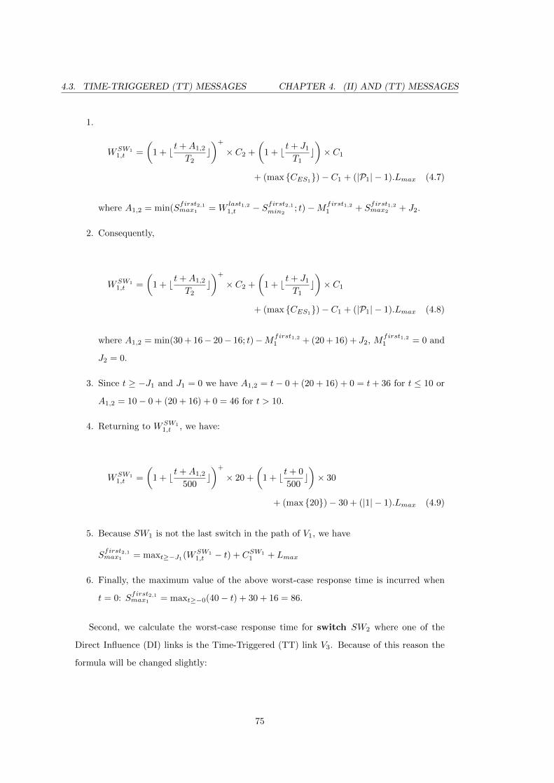
4.3. TIME-TRIGGERED (TT) MESSAGES CHAPTER 4. (II) AND (TT) MESSAGES
1.
WSW11,t =
(1 + b t+A1,2
T2c)+
× C2 +
(1 + b t+ J1
T1c)× C1
+ (max {CES1})− C1 + (|P1| − 1).Lmax (4.7)
where A1,2 = min(Sfirst2,1max1 = W
last1,21,t − Sfirst2,1
min2; t)−Mfirst1,2
1 + Sfirst1,2max2 + J2.
2. Consequently,
WSW11,t =
(1 + b t+A1,2
T2c)+
× C2 +
(1 + b t+ J1
T1c)× C1
+ (max {CES1})− C1 + (|P1| − 1).Lmax (4.8)
where A1,2 = min(30 + 16− 20− 16; t)−Mfirst1,21 + (20 + 16) + J2, M
first1,21 = 0 and
J2 = 0.
3. Since t ≥ −J1 and J1 = 0 we have A1,2 = t− 0 + (20 + 16) + 0 = t+ 36 for t ≤ 10 or
A1,2 = 10− 0 + (20 + 16) + 0 = 46 for t > 10.
4. Returning to WSW11,t , we have:
WSW11,t =
(1 + b t+A1,2
500c)+
× 20 +
(1 + b t+ 0
500c)× 30
+ (max {20})− 30 + (|1| − 1).Lmax (4.9)
5. Because SW1 is not the last switch in the path of V1, we have
Sfirst2,1max1 = maxt≥−J1
(WSW11,t − t) + CSW1
1 + Lmax
6. Finally, the maximum value of the above worst-case response time is incurred when
t = 0: Sfirst2,1max1 = maxt≥−0(40− t) + 30 + 16 = 86.
Second, we calculate the worst-case response time for switch SW2 where one of the
Direct Influence (DI) links is the Time-Triggered (TT) link V3. Because of this reason the
formula will be changed slightly:
75
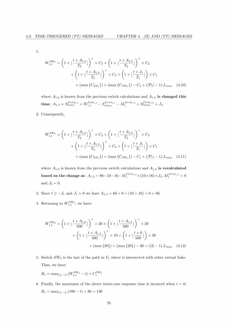
4.3. TIME-TRIGGERED (TT) MESSAGES CHAPTER 4. (II) AND (TT) MESSAGES
1.
WSW21,t =
(1 + b t+A1,2
T2c)+
× C2 +
(1 + b t+A1,2
T2c)+
× C2
+
(1 + b t+A1,3
T3c)+
× C3 +
(1 + b t+ J1
T1c)× C1
+ (max {CES1}) + (max {CSW1})− C1 + (|P1| − 1).Lmax (4.10)
where A1,2 is known from the previous switch calculations and A1,3 is changed this
time: A1,3 = Sfirst3,1max1 = W
last1,31,t − Sfirst3,1
min3−Mfirst1,3
1 + Sfirst1,3max3 + J3.
2. Consequently,
WSW21,t =
(1 + b t+A1,2
T2c)+
× C2 +
(1 + b t+A1,2
T2c)+
× C2
+
(1 + b t+A1,3
T3c)+
× C3 +
(1 + b t+ J1
T1c)× C1
+ (max {CES1}) + (max {CSW1
})− C1 + (|P1| − 1).Lmax (4.11)
where A1,2 is known from the previous switch calculations and A1,3 is recalculated
based on the change as: A1,3 = 86−10−16−Mfirst1,31 +(10+16)+J3, M
first1,31 = 0
and J3 = 0.
3. Since t ≥ −J1 and J1 = 0 we have A1,3 = 60 + 0 + (10 + 16) + 0 = 86.
4. Returning to WSW21,t , we have:
WSW21,t =
(1 + b t+A1,2
500c)+
× 20 +
(1 + b t+A1,2
500c)+
× 20
+
(1 + b t+A1,3
500c)+
× 10 +
(1 + b t+ 0
500c)× 30
+ (max {20}) + (max {20})− 30 + (|2| − 1).Lmax (4.12)
5. Switch SW2 is the last of the path in V1 where is intersected with other virtual links.
Thus, we have:
R1 = maxt≥−J1(WSW2
1,t − t) + CSW21
6. Finally, the maximum of the above worst-case response time is incurred when t = 0:
R1 = maxt≥−J1(106− t) + 30 = 136
76
4.3. TIME-TRIGGERED (TT) MESSAGES CHAPTER 4. (II) AND (TT) MESSAGES
This result is exactly the same as the one calculated for systems without Time-Triggered
(TT) messages. Furthermore, we did not find this t value for which the result is different.
There is additional requirement for the BAG parameter. It is caused by two consequen-
tial transmissions of Time-Triggered (TT) messages. The problem is depicted in Figure 4.4.
When a Time-Triggered (TT) message is transmitted, it takes precedence over the rest of
the traffic. If the transmissions are quite often (the case on left), this means shorter BAG
value, then queueing of messages from Rate-Constrained (RC) type may occur. In fact, the
queueing can be so long that a new scheduled Time-Traffic (TT) message can arrive for
transmission before the queue is processed. In this way the currently transmitted messages
will be suspended and possibly never transmitted. This will lead to buffer overflow and
infeasibility of the system.
Figure 4.4: BAG of Time-Triggered (TT) messages
The network architect should resolve the presented problem offline while the network is
in design phase.
77
Chapter 5
Evaluation
5.1 Introduction
In this chapter we provide an evaluation of the problem featured in this project. We do it
in several steps.
First, we introduce a larger example to which the same computations regarding the
Trajectory approach are applied. The example contains compound hardware configuration
with several virtual links (as application configuration) that have Direct Influence (DI)
virtual links. In section 4.2 we concluded that only the Direct Influence (DI) virtual links
from three presented classes (Direct Influence (DI), Indirect Influence (II) and No Influence)
have impact on the worst-case response times.
Second, we do a comparison between our approach and the Holistic one and conclude
the domination of the Trajectory approach. The parallel between both approaches is based
on the worst-case response times achieved. The comparison considers two examples, the one
presented in section 3.5 and the other presented in the current chapter.
Finally, the chapter also includes additional evaluation of the dependency of the parame-
ters related to the calculations. The intention is to present how the parameters of the virtual
link can influence the worst-case response times.
78
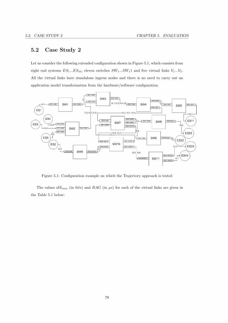
5.2. CASE STUDY 2 CHAPTER 5. EVALUATION
5.2 Case Study 2
Let us consider the following extended configuration shown in Figure 5.1, which consists from
eight end systems ES1...ES44, eleven switches SW1...SW11 and five virtual links V1...V5.
All the virtual links have standalone ingress nodes and there is no need to carry out an
application model transformation from the hardware/software configuration.
Figure 5.1: Configuration example on which the Trajectory approach is tested
The values ofSmax (in bits) and BAG (in µs) for each of the virtual links are given in
the Table 5.1 below:
79
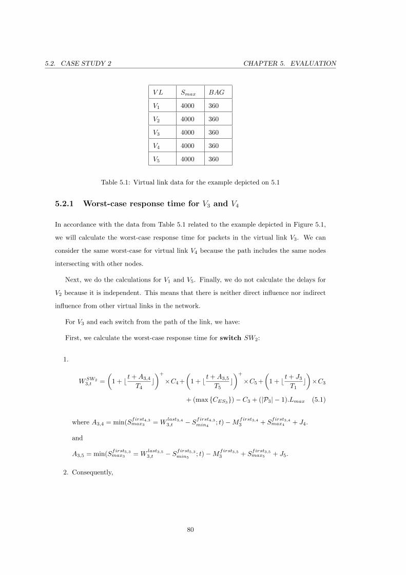
5.2. CASE STUDY 2 CHAPTER 5. EVALUATION
V L Smax BAG
V1 4000 360
V2 4000 360
V3 4000 360
V4 4000 360
V5 4000 360
Table 5.1: Virtual link data for the example depicted on 5.1
5.2.1 Worst-case response time for V3 and V4
In accordance with the data from Table 5.1 related to the example depicted in Figure 5.1,
we will calculate the worst-case response time for packets in the virtual link V3. We can
consider the same worst-case for virtual link V4 because the path includes the same nodes
intersecting with other nodes.
Next, we do the calculations for V1 and V5. Finally, we do not calculate the delays for
V2 because it is independent. This means that there is neither direct influence nor indirect
influence from other virtual links in the network.
For V3 and each switch from the path of the link, we have:
First, we calculate the worst-case response time for switch SW2:
1.
WSW23,t =
(1 + b t+A3,4
T4c)+
×C4 +
(1 + b t+A3,5
T5c)+
×C5 +
(1 + b t+ J3
T1c)×C3
+ (max {CES3})− C3 + (|P3| − 1).Lmax (5.1)
where A3,4 = min(Sfirst4,3max3 = W
last3,43,t − Sfirst4,3
min4; t)−Mfirst3,4
3 + Sfirst3,4max4 + J4.
and
A3,5 = min(Sfirst5,3max3 = W
last3,53,t − Sfirst5,3
min5; t)−Mfirst3,5
3 + Sfirst3,5max5 + J5.
2. Consequently,
80
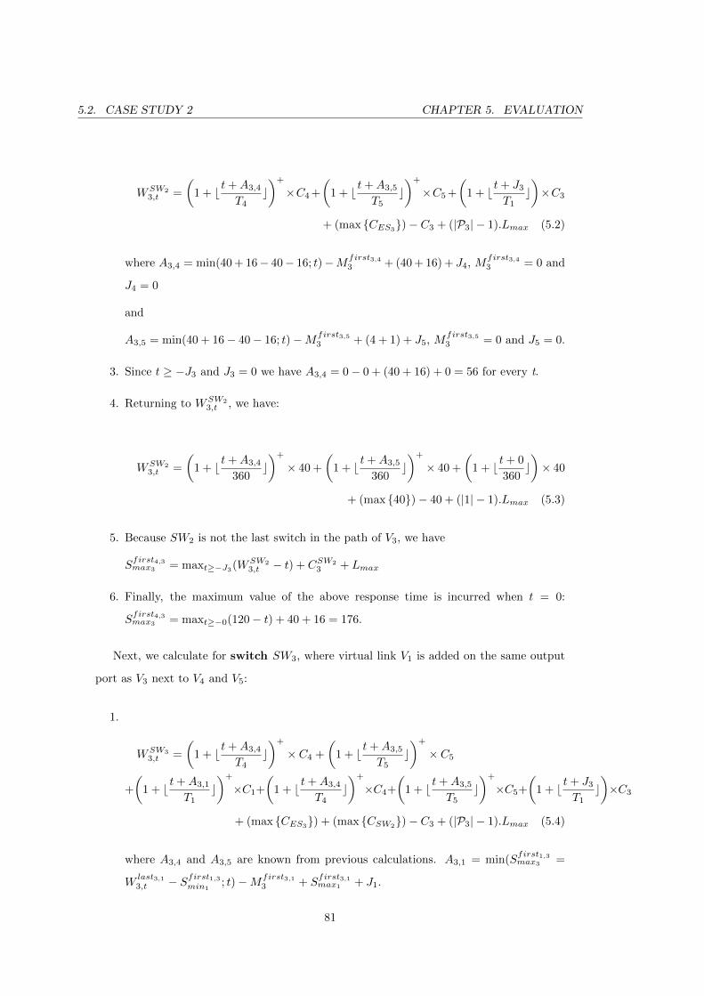
5.2. CASE STUDY 2 CHAPTER 5. EVALUATION
WSW23,t =
(1 + b t+A3,4
T4c)+
×C4 +
(1 + b t+A3,5
T5c)+
×C5 +
(1 + b t+ J3
T1c)×C3
+ (max {CES3})− C3 + (|P3| − 1).Lmax (5.2)
where A3,4 = min(40 + 16− 40− 16; t)−Mfirst3,43 + (40 + 16) + J4, M
first3,43 = 0 and
J4 = 0
and
A3,5 = min(40 + 16− 40− 16; t)−Mfirst3,53 + (4 + 1) + J5, M
first3,53 = 0 and J5 = 0.
3. Since t ≥ −J3 and J3 = 0 we have A3,4 = 0− 0 + (40 + 16) + 0 = 56 for every t.
4. Returning to WSW23,t , we have:
WSW23,t =
(1 + b t+A3,4
360c)+
× 40 +
(1 + b t+A3,5
360c)+
× 40 +
(1 + b t+ 0
360c)× 40
+ (max {40})− 40 + (|1| − 1).Lmax (5.3)
5. Because SW2 is not the last switch in the path of V3, we have
Sfirst4,3max3 = maxt≥−J3
(WSW23,t − t) + CSW2
3 + Lmax
6. Finally, the maximum value of the above response time is incurred when t = 0:
Sfirst4,3max3 = maxt≥−0(120− t) + 40 + 16 = 176.
Next, we calculate for switch SW3, where virtual link V1 is added on the same output
port as V3 next to V4 and V5:
1.
WSW33,t =
(1 + b t+A3,4
T4c)+
× C4 +
(1 + b t+A3,5
T5c)+
× C5
+
(1 + b t+A3,1
T1c)+
×C1+
(1 + b t+A3,4
T4c)+
×C4+
(1 + b t+A3,5
T5c)+
×C5+
(1 + b t+ J3
T1c)×C3
+ (max {CES3}) + (max {CSW2
})− C3 + (|P3| − 1).Lmax (5.4)
where A3,4 and A3,5 are known from previous calculations. A3,1 = min(Sfirst1,3max3 =
Wlast3,13,t − Sfirst1,3
min1; t)−Mfirst3,1
3 + Sfirst3,1max1 + J1.
81
5.2. CASE STUDY 2 CHAPTER 5. EVALUATION
2. Consequently,
WSW23,t =
(1 + b t+A3,4
T4c)+
× C4 +
(1 + b t+A3,5
T5c)+
× C5
+
(1 + b t+A3,1
T1c)+
×C1+
(1 + b t+A3,4
T4c)+
×C4+
(1 + b t+A3,5
T5c)+
×C5+
(1 + b t+ J3
T1c)×C3
+ (max {CES3}) + (max {CSW2})− C3 + (|P3| − 1).Lmax (5.5)
where A3,4 and A3,5 are known from previous calculations. A3,1 = min(176 − 40 −
16; t)−Mfirst3,13 + (40 + 16) + J1, M
first3,13 = 0 and J1 = 0.
3. Since t ≥ −J3 and J3 = 0 we have A3,1 = t− 0 + (40 + 16) + 0 = t+ 56 for t ≤ 120 or
A3,1 = 0− 0 + (40 + 16) + 0 = 56 for t 120.
4. Returning to WSW23,t , we have:
WSW33,t =
(1 + b t+A3,4
360c)+
× 40 +
(1 + b t+A3,5
360c)+
× 40
+
(1 + b t+A3,1
360c)+
×40+
(1 + b t+A3,4
360c)+
×40+
(1 + b t+A3,5
360c)+
×40+
(1 + b t+ 0
360c)×40
+ (max {40}) + (max {40})− 40 + (|2| − 1).Lmax (5.6)
5. Because SW3 is not the last switch in the path of V3, we have
Sfirst1,3max3 = maxt≥−J3
(WSW33,t − t) + CSW2
3 + Lmax
6. Finally, the maximum value of the above response time is incurred when t = 0:
Sfirst1,3max3 = maxt≥−0(296− t) + 40 + 16 = 352.
Next, we calculate the worst-case response time for switch SW4, where V4 and V5 are
the only other links on the same output port as V3:
82
5.2. CASE STUDY 2 CHAPTER 5. EVALUATION
1.
WSW43,t =
(1 + b t+A3,4
T4c)+
× C4 +
(1 + b t+A3,5
T5c)+
× C5
+
(1 + b t+A3,1
T1c)+
× C1 +
(1 + b t+A3,4
T4c)+
× C4 +
(1 + b t+A3,5
T5c)+
× C5
+
(1 + b t+A3,4
T4c)+
× C4 +
(1 + b t+A3,5
T5c)+
× C5
+
(1 + b t+ J3
T1c)×C3+(max {CES3
})+(max {CSW2})+(max {CSW3
})−C3+(|P3|−1).Lmax
(5.7)
where A3,4, A3,5 and A3,1 are known from previous calculations.
2. Returning to WSW43,t , we have:
WSW43,t =
(1 + b t+A3,4
360c)+
× 40 +
(1 + b t+A3,5
360c)+
× 40
+
(1 + b t+A3,1
360c)+
× 40 +
(1 + b t+A3,4
360c)+
× 40 +
(1 + b t+A3,5
360c)+
× 40
+
(1 + b t+A3,4
360c)+
× 40 +
(1 + b t+A3,5
360c)+
× 40
+
(1 + b t+ 0
360c)×40 + (max {40}) + (max {40}) + (max {40})−40 + (|3|−1).Lmax
(5.8)
3. Finally, the maximum value of the above response time is incurred when t = 0:
WSW43,t = maxt≥−0(432− t) + 40 + 16 = 488.
Next, we calculate the worst-case response time for switch SW7, where V4 is the only
link on the same output port as V3:
83
5.2. CASE STUDY 2 CHAPTER 5. EVALUATION
1.
WSW73,t =
(1 + b t+A3,4
T4c)+
× C4 +
(1 + b t+A3,5
T5c)+
× C5
+
(1 + b t+A3,1
T1c)+
× C1 +
(1 + b t+A3,4
T4c)+
× C4 +
(1 + b t+A3,5
T5c)+
× C5
+
(1 + b t+A3,4
T4c)+
× C4 +
(1 + b t+A3,5
T5c)+
× C5
+
(1 + b t+A3,4
T4c)+
× C4 +
(1 + b t+ J3
T1c)× C3
+(max {CES3})+(max {CSW2})+(max {CSW3})+(max {CSW4})−C3+(|P3|−1).Lmax
(5.9)
2. where A3,4, A3,5 and A3,1 are known from previous calculations.
3. Returning to WSW73,t , we have:
WSW73,t =
(1 + b t+A3,4
360c)+
× 40 +
(1 + b t+A3,5
360c)+
× 40
+
(1 + b t+A3,1
360c)+
× 40 +
(1 + b t+A3,4
360c)+
× 40 +
(1 + b t+A3,5
360c)+
× 40
+
(1 + b t+A3,4
360c)+
× 40 +
(1 + b t+A3,5
360c)+
× 40
+
(1 + b t+A3,4
360c)+
× 40 +
(1 + b t+ 0
360c)× 40
+ (max {40}) + (max {40}) + (max {40})− 40 + (|4| − 1).Lmax (5.10)
4. Finally, the maximum value of the above response time is incurred when t = 0:
WSW73,t = maxt≥−0(528− t) + 40 + 16 = 584.
By analogy WSW103,t = 640 for t = 0.
Finally, the rest of the path of virtual links is not intersected with any other virtual links.
Thus, we have:
R3 = maxt≥−J3(WSW10
3,t − t) + CSW103 (640− t) + 40 = 680
Virtual link V3 has one more switch in its path. This is switch SW1, which is crossed
without any influence from another virtual link. The final result for R3 is:
R∗3 = R3 + Lmax + CSW113 + Lmax = 61 + 16 + 40 + 16 = 752
84
5.2. CASE STUDY 2 CHAPTER 5. EVALUATION
5.2.2 Worst-case response time for V1
The path of virtual link V1 crosses switch SW1 at the beginning of its path, independently,
without any direct or indirect influence from other virtual links. The same can be observed
for the last two switches SW4 and SW5. Thus, we can formulate the Trajectory approach
only for SW3:
1.
WSW31,t =
(1 + b t+A1,3
T3c)+
×C3+
(1 + b t+A1,4
T4c)+
×C4+
(1 + b t+A1,5
T5c)+
×C5
+
(1 + b t+ J1
T1c)× C1 + (max {CES1
})− C1 + (|P1| − 1).Lmax (5.11)
where A1,3, A1,4 and A1,5 are known from previous calculations.
2. Returning to WSW31,t , we have:
WSW31,t =
(1 + b t+A1,3
360c)+
×40+
(1 + b t+A1,4
360c)+
×40+
(1 + b t+A1,5
360c)+
×40
+
(1 + b t+ 0
360c)× 40 + (max {40})− 40 + (|P1| − 1).Lmax (5.12)
3. Finally, the maximum value of the above response time is incurred when t = 0:
WSW31,t = maxt≥−0(160− t) + 40 + 16 = 216.
Finally, the rest of the path of virtual links is not intersected with any other virtual links.
Thus, we have:
R1 = maxt≥−J1(WSW3
1,t − t) + CSW31 (216− t) + 40 = 256
As previously mentioned, virtual link V1 contains additional switches in its path. These
are switches SW1, SW4, SW5, which are crossed without any influence from another virtual
link. The final result for R1 is:
R∗1 = R1 +Lmax +CSW11 +Lmax +CSW4
1 +Lmax +CSW51 +Lmax = 256 + 16 + 40 + 16 +
40 + 16 + 40 + 16 = 384
5.2.3 Worst-case response time for V5
For V5 and each switch in the path of the link, we have:
85
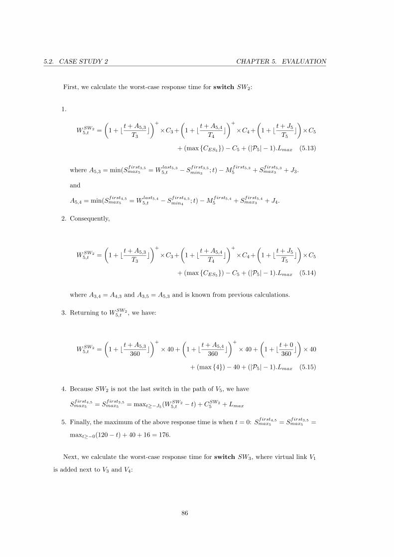
5.2. CASE STUDY 2 CHAPTER 5. EVALUATION
First, we calculate the worst-case response time for switch SW2:
1.
WSW25,t =
(1 + b t+A5,3
T3c)+
×C3 +
(1 + b t+A5,4
T4c)+
×C4 +
(1 + b t+ J5
T5c)×C5
+ (max {CES5})− C5 + (|P5| − 1).Lmax (5.13)
where A5,3 = min(Sfirst3,5max5 = W
last5,35,t − Sfirst3,5
min3; t)−Mfirst5,3
5 + Sfirst5,3max3 + J3.
and
A5,4 = min(Sfirst4,5max5 = W
last5,45,t − Sfirst4,5
min4; t)−Mfirst5,4
5 + Sfirst5,4max3 + J4.
2. Consequently,
WSW25,t =
(1 + b t+A5,3
T3c)+
×C3 +
(1 + b t+A5,4
T4c)+
×C4 +
(1 + b t+ J5
T5c)×C5
+ (max {CES5})− C5 + (|P5| − 1).Lmax (5.14)
where A3,4 = A4,3 and A3,5 = A5,3 and is known from previous calculations.
3. Returning to WSW25,t , we have:
WSW25,t =
(1 + b t+A5,3
360c)+
× 40 +
(1 + b t+A5,4
360c)+
× 40 +
(1 + b t+ 0
360c)× 40
+ (max {4})− 40 + (|P5| − 1).Lmax (5.15)
4. Because SW2 is not the last switch in the path of V5, we have
Sfirst4,5max5 = S
first3,5max5 = maxt≥−J5
(WSW25,t − t) + CSW2
5 + Lmax
5. Finally, the maximum of the above response time is when t = 0: Sfirst4,5max5 = S
first3,5max5 =
maxt≥−0(120− t) + 40 + 16 = 176.
Next, we calculate the worst-case response time for switch SW3, where virtual link V1
is added next to V3 and V4:
86
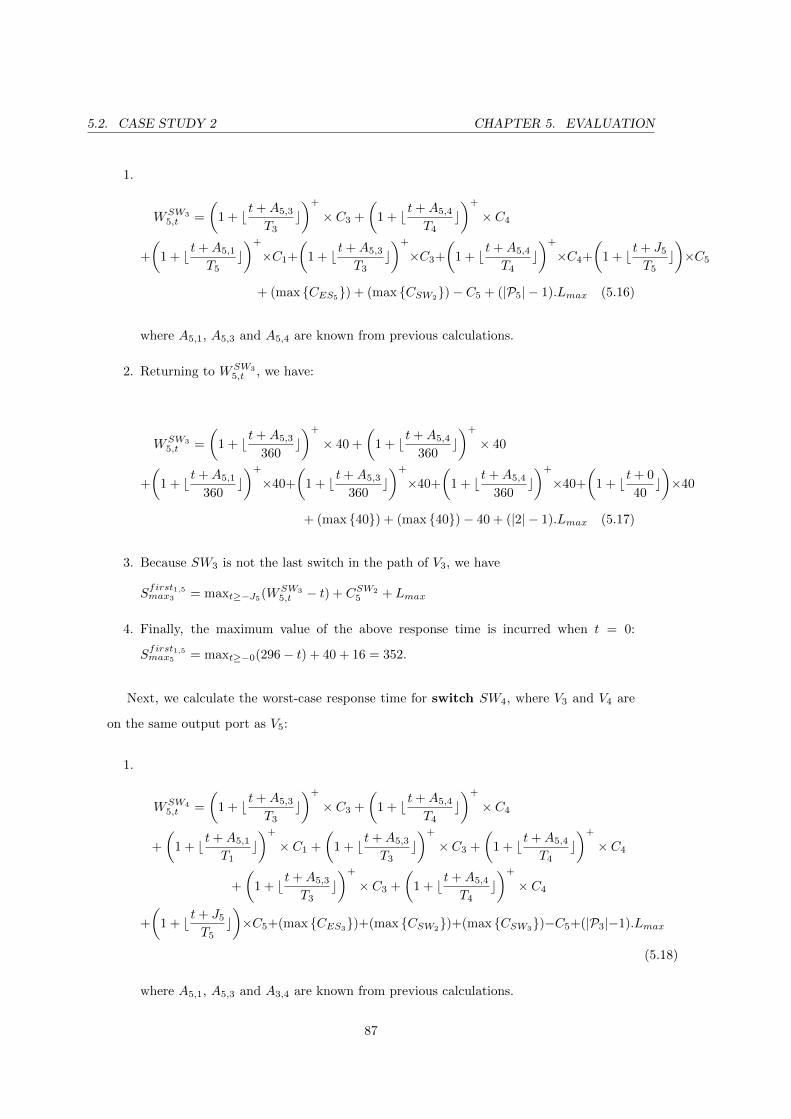
5.2. CASE STUDY 2 CHAPTER 5. EVALUATION
1.
WSW35,t =
(1 + b t+A5,3
T3c)+
× C3 +
(1 + b t+A5,4
T4c)+
× C4
+
(1 + b t+A5,1
T5c)+
×C1+
(1 + b t+A5,3
T3c)+
×C3+
(1 + b t+A5,4
T4c)+
×C4+
(1 + b t+ J5
T5c)×C5
+ (max {CES5}) + (max {CSW2
})− C5 + (|P5| − 1).Lmax (5.16)
where A5,1, A5,3 and A5,4 are known from previous calculations.
2. Returning to WSW35,t , we have:
WSW35,t =
(1 + b t+A5,3
360c)+
× 40 +
(1 + b t+A5,4
360c)+
× 40
+
(1 + b t+A5,1
360c)+
×40+
(1 + b t+A5,3
360c)+
×40+
(1 + b t+A5,4
360c)+
×40+
(1 + b t+ 0
40c)×40
+ (max {40}) + (max {40})− 40 + (|2| − 1).Lmax (5.17)
3. Because SW3 is not the last switch in the path of V3, we have
Sfirst1,5max3 = maxt≥−J5
(WSW35,t − t) + CSW2
5 + Lmax
4. Finally, the maximum value of the above response time is incurred when t = 0:
Sfirst1,5max5 = maxt≥−0(296− t) + 40 + 16 = 352.
Next, we calculate the worst-case response time for switch SW4, where V3 and V4 are
on the same output port as V5:
1.
WSW45,t =
(1 + b t+A5,3
T3c)+
× C3 +
(1 + b t+A5,4
T4c)+
× C4
+
(1 + b t+A5,1
T1c)+
× C1 +
(1 + b t+A5,3
T3c)+
× C3 +
(1 + b t+A5,4
T4c)+
× C4
+
(1 + b t+A5,3
T3c)+
× C3 +
(1 + b t+A5,4
T4c)+
× C4
+
(1 + b t+ J5
T5c)×C5+(max {CES3
})+(max {CSW2})+(max {CSW3
})−C5+(|P3|−1).Lmax
(5.18)
where A5,1, A5,3 and A3,4 are known from previous calculations.
87
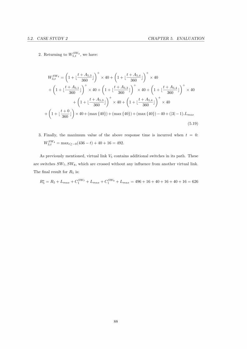
5.2. CASE STUDY 2 CHAPTER 5. EVALUATION
2. Returning to WSW45,t , we have:
WSW43,t =
(1 + b t+A5,3
360c)+
× 40 +
(1 + b t+A5,4
360c)+
× 40
+
(1 + b t+A5,1
360c)+
× 40 +
(1 + b t+A5,3
360c)+
× 40 +
(1 + b t+A5,4
360c)+
× 40
+
(1 + b t+A5,3
360c)+
× 40 +
(1 + b t+A5,4
360c)+
× 40
+
(1 + b t+ 0
360c)×40 + (max {40}) + (max {40}) + (max {40})−40 + (|3|−1).Lmax
(5.19)
3. Finally, the maximum value of the above response time is incurred when t = 0:
WSW43,t = maxt≥−0(436− t) + 40 + 16 = 492.
As previously mentioned, virtual link V5 contains additional switches in its path. These
are switches SW7, SW8, which are crossed without any influence from another virtual link.
The final result for R5 is:
R∗5 = R5 + Lmax +CSW71 + Lmax +CSW8
1 + Lmax = 496 + 16 + 40 + 16 + 40 + 16 = 626
88
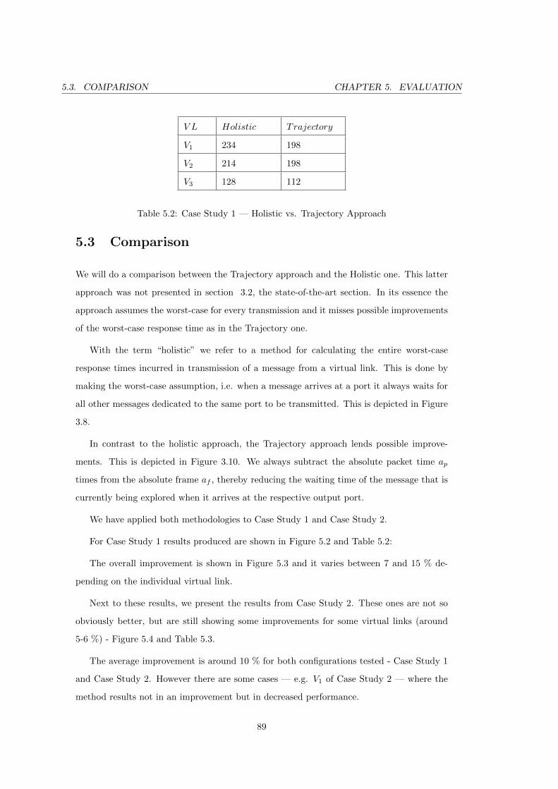
5.3. COMPARISON CHAPTER 5. EVALUATION
V L Holistic Trajectory
V1 234 198
V2 214 198
V3 128 112
Table 5.2: Case Study 1 — Holistic vs. Trajectory Approach
5.3 Comparison
We will do a comparison between the Trajectory approach and the Holistic one. This latter
approach was not presented in section 3.2, the state-of-the-art section. In its essence the
approach assumes the worst-case for every transmission and it misses possible improvements
of the worst-case response time as in the Trajectory one.
With the term “holistic” we refer to a method for calculating the entire worst-case
response times incurred in transmission of a message from a virtual link. This is done by
making the worst-case assumption, i.e. when a message arrives at a port it always waits for
all other messages dedicated to the same port to be transmitted. This is depicted in Figure
3.8.
In contrast to the holistic approach, the Trajectory approach lends possible improve-
ments. This is depicted in Figure 3.10. We always subtract the absolute packet time ap
times from the absolute frame af , thereby reducing the waiting time of the message that is
currently being explored when it arrives at the respective output port.
We have applied both methodologies to Case Study 1 and Case Study 2.
For Case Study 1 results produced are shown in Figure 5.2 and Table 5.2:
The overall improvement is shown in Figure 5.3 and it varies between 7 and 15 % de-
pending on the individual virtual link.
Next to these results, we present the results from Case Study 2. These ones are not so
obviously better, but are still showing some improvements for some virtual links (around
5-6 %) - Figure 5.4 and Table 5.3.
The average improvement is around 10 % for both configurations tested - Case Study 1
and Case Study 2. However there are some cases — e.g. V1 of Case Study 2 — where the
method results not in an improvement but in decreased performance.
89
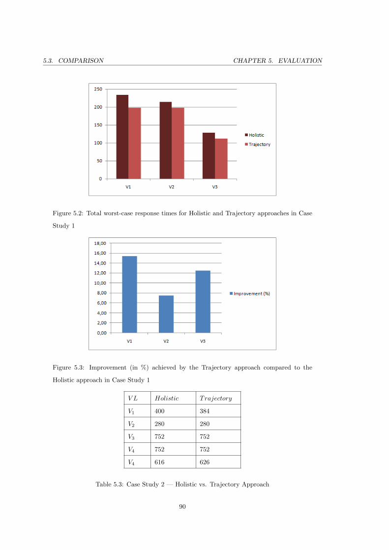
5.3. COMPARISON CHAPTER 5. EVALUATION
Figure 5.2: Total worst-case response times for Holistic and Trajectory approaches in Case
Study 1
Figure 5.3: Improvement (in %) achieved by the Trajectory approach compared to the
Holistic approach in Case Study 1
V L Holistic Trajectory
V1 400 384
V2 280 280
V3 752 752
V4 752 752
V4 616 626
Table 5.3: Case Study 2 — Holistic vs. Trajectory Approach
90
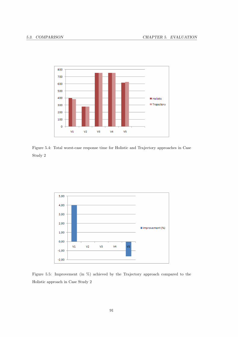
5.3. COMPARISON CHAPTER 5. EVALUATION
Figure 5.4: Total worst-case response time for Holistic and Trajectory approaches in Case
Study 2
Figure 5.5: Improvement (in %) achieved by the Trajectory approach compared to the
Holistic approach in Case Study 2
91
Chapter 6
Implementation
6.1 Introduction
In this chapter we will explain details about our programming implementation of the cal-
culations that we have developed and presented so far. The main code structures and
functionalities of the algorithms are demonstrated. All the source code is written in Java.
92
6.2. INPUT MODEL CHAPTER 6. IMPLEMENTATION
6.2 Input model
The entire program is modelled by the help of 4 configuration files in GraphML[34] file
format.
� architectureGraphXXX.graphml — The file is related to the hardware architec-
ture (section 2.2). It contains description of all end systems, switches, ports of switches
and links between end systems and switches.
� configurationMXXX.graphml — The file contains information about all parame-
ters related to a message sent from an end system. Multiple messages can be assigned
to a virtual link. Modifiable parameters of a message are: type of the message, prior-
ity, size, period (equal to virtual link’s BAG, deadline (usually is set as equal to the
period).
� configurationVLXXX.graphml — The file is responsible for the configuration of
the virtual links. Each virtual link has BAG, Smax and Smin parameter values. This
setup also contains a path parameter value, which can be unicast or multicast.
� configurationTTXXX.graphml — The file contains the exact times of emissions
by Time-Triggered (TT) messages in the system environment.
93
6.3. PRELIMINARY SETUP CHAPTER 6. IMPLEMENTATION
6.3 Preliminary setup
The input is read from the GraphML files described in the above section. Consequently
from the first file are build the objects which represents the end nodes, the switches, and
the ports of the respective switches. The next task is to distribute the virtual link informa-
tion (read from file configurationVLXXX.graphml). Some of the objects (e.g. the end
systems) contains containers which keep track of the incoming and outcoming virtual links.
A process fills up the required information for them. In parallel of this operation are done
validations of the the virtual links paths. Finally the messages are read from file configu-
rationMXXX.graphml and assigned to the respective components from the configuration
(i.e. end nodes and ports of the switches).
The preliminary setup finishes with printout of the loaded configuration. This is done
by showing of all elements described in the configuration files in appropriate order (i.e. from
hardware perspective of view — node by node and from application point of view — virtual
link by virtual link). In these phase is done also validation checking of the input and if the
printout is successful all the validations are passed affirmatively.
94
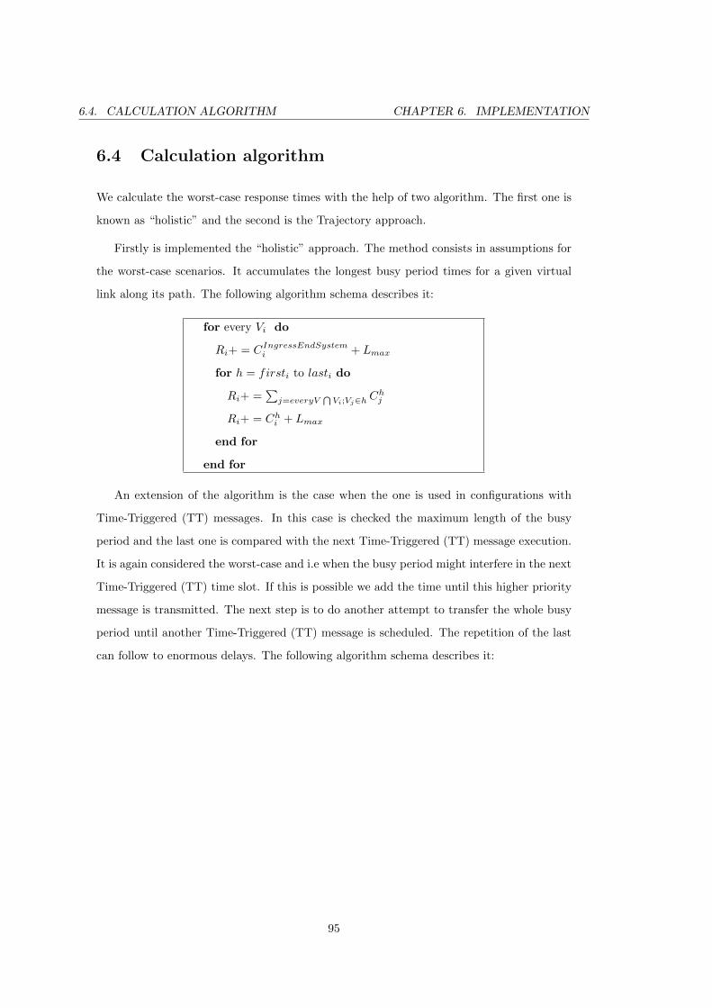
6.4. CALCULATION ALGORITHM CHAPTER 6. IMPLEMENTATION
6.4 Calculation algorithm
We calculate the worst-case response times with the help of two algorithm. The first one is
known as “holistic” and the second is the Trajectory approach.
Firstly is implemented the “holistic” approach. The method consists in assumptions for
the worst-case scenarios. It accumulates the longest busy period times for a given virtual
link along its path. The following algorithm schema describes it:
for every Vi do
Ri+ = CIngressEndSystemi + Lmax
for h = firsti to lasti do
Ri+ =∑
j=everyV⋂
Vi;Vj∈h Chj
Ri+ = Chi + Lmax
end for
end for
An extension of the algorithm is the case when the one is used in configurations with
Time-Triggered (TT) messages. In this case is checked the maximum length of the busy
period and the last one is compared with the next Time-Triggered (TT) message execution.
It is again considered the worst-case and i.e when the busy period might interfere in the next
Time-Triggered (TT) time slot. If this is possible we add the time until this higher priority
message is transmitted. The next step is to do another attempt to transfer the whole busy
period until another Time-Triggered (TT) message is scheduled. The repetition of the last
can follow to enormous delays. The following algorithm schema describes it:
95
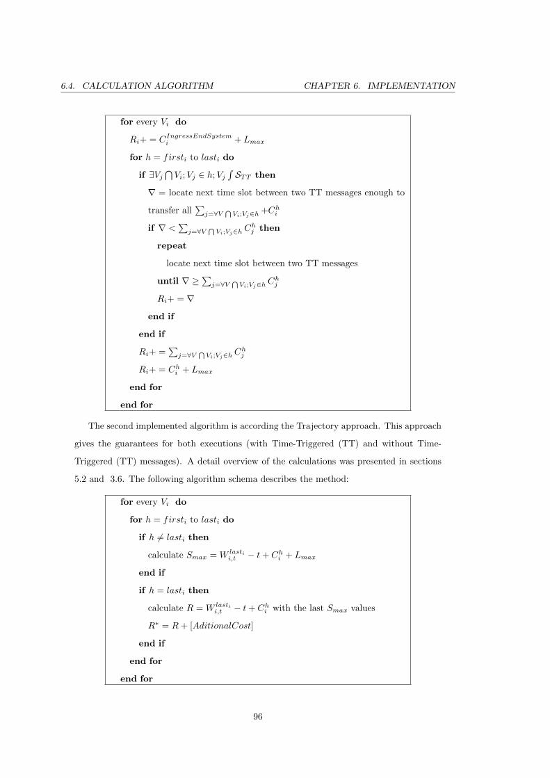
6.4. CALCULATION ALGORITHM CHAPTER 6. IMPLEMENTATION
for every Vi do
Ri+ = CIngressEndSystemi + Lmax
for h = firsti to lasti do
if ∃Vj⋂Vi;Vj ∈ h;Vj
∫STT then
∇ = locate next time slot between two TT messages enough to
transfer all∑
j=∀V⋂
Vi;Vj∈h +Chi
if ∇ <∑
j=∀V⋂
Vi;Vj∈h Chj then
repeat
locate next time slot between two TT messages
until ∇ ≥∑
j=∀V⋂
Vi;Vj∈h Chj
Ri+ = ∇
end if
end if
Ri+ =∑
j=∀V⋂
Vi;Vj∈h Chj
Ri+ = Chi + Lmax
end for
end for
The second implemented algorithm is according the Trajectory approach. This approach
gives the guarantees for both executions (with Time-Triggered (TT) and without Time-
Triggered (TT) messages). A detail overview of the calculations was presented in sections
5.2 and 3.6. The following algorithm schema describes the method:
for every Vi do
for h = firsti to lasti do
if h 6= lasti then
calculate Smax = W lastii,t − t+ Ch
i + Lmax
end if
if h = lasti then
calculate R = W lastii,t − t+ Ch
i with the last Smax values
R∗ = R+ [AditionalCost]
end if
end for
end for
96
Chapter 7
Conclusion
Embedded systems exploration is related to the creation of safety-critical applications, where
precise requirements are involved. Many safety-critical applications exist in heterogeneous
environments and the production of parts for them is often shared between different vendors.
All this makes the achievement of common scheduling of the shared tasks difficult.
One universal solution is offered by the TTEthernet networks. This technology offers
a medium at communication level where several types of messages can be handled: Time-
Triggered (TT) messages, Rate-Constrained (RC) messages and Best-Effort (BE) messages.
This helps in situations such as the above where the requirements for different tasks(e.g.,
safety-critical vs. non-safety critical) have to be implemented on the same platform. A
special case of the TTEthernet is the AFDX network where only Rate-Constrained (RC)
messages occur.
We propose an extension of the Trajectory approach introduced in [26], [27], [28] and [29]
applied firstly to an AFDX network. Originally, this approach was addressed to distributed
networks which contains FP/DP ∗ (fixed priority and dynamic priority established on the
first node visited in the network). This scheduling has two forms - FP/FIFO∗14 and
FP/EDF ∗15. Because of its nature, the former is compatible with the AFDX network
scheduling, which provides FIFO functionality for Rate-Constrained (RC) messages.
We did the calculations for the configuration that contains virtual links with Rate-
Constrained (RC) messages, influenced only by Direct Influence (DI) virtual links. After-
14Fixed Priority / First In, First Out15Fixed Priority / Earliest Deadline First
97
CHAPTER 7. CONCLUSION
wards, Indirect Influence (II) virtual links were attached and the results were recalculated.
The results after recalculation showed that the method is not dependent on these links.
Next, we have introduced the Time-Triggered (TT) class of messages, which transformed
the network to TTEthernet network. We have substituted some Rate-Constrained (RC)
messages with Time-Triggered (TT) ones. The corresponding formula was changed and the
calculations were redone.
Finally, there were some recommendations about the integration of Time-Triggered (TT)
messages with the Rate-Constrained (RC) traffic.
The method was evaluated for a larger configuration, which showed satisfactory results
for some of the virtual links. Additionally, there were comments about the parameter
dependency of the formula parameters.
In future, the importance of the research work for these networks (TTEthernet / AFDX)
will be enormous. The study throughout this thesis is based on a number of assumptions
simplifying the various lines of research in this area. We concentrated on devising a method
for easy calculation of the end-to-end delays of the traffic (Time-Triggered (TT) and Rate-
Constrained (RC)) and we have not investigated specific events in the network that could
change these end-to-end delays. By specific events, we mean any event in the course of
normal operation or one caused by a failure in the network. Therefore and in addition, the
work presented in this project can be extended in these examples to aspects such as the
following:
� There is a need to research the influence of the the computation time inside the end
nodes. An end node is usually subject to contention from several logical partitions
that have to cooperate over the usage of the single resource CPU
� Another area which can be improved is the intercommunication between different
synchronization domains in these networks. As previously explained, the topology
could be complex, and this calls for additional assumptions for the calculations of the
worst-case response times
� The third domain of future work is the integration of the Best-Effort (BE) traffic
with the rest of the ongoing traffic (Rate-Constrained (RC) and Time-Triggered (TT)
traffic). A quantitative or quality method should be developed which can show or
predict the trends of the behaviour of this traffic class.
98
CHAPTER 7. CONCLUSION
These few prospects show just how much more work needs to be done in this area.
The recent trend for using AFDX / TTEthernet networks in the avionics industry requires
detailed study of their performance and even more higher focus on the certification of these
networks. Therefore, any methods developed will be welcomed for contributing to the precise
control of these networks (trajectory, network calculus, model approach and etc).
99
Bibliography
[1] Henning Butz Open Integrated Modular Avionic (IMA): State of the Art and future
Development Road Map at Airbus Deutschland
[2] Richard L. Alena, John Ossenfort, Andre Goforth, Fernando Figueroa Communications
for Integrated Modular Avionics
[3] RenAndre L.C. Eveleens Integrated Modular Avionics Development Guidance and Cer-
tification Considerations
[4] Jean-Bernard ITIER A380 Integrated Modular Avionics - Presentation
[5] ARINC http://www.arinc.com
[6] ARINC 664 Aircraft Data Network, Part 7, Avionics Full Duplex Switched Ethernet
(AFDX) Network, 2005
[7] General Electric AFDX/ARINC 664 Protocol, Tutorial
[8] Xillinx Architecting ARINC 664, Parr 7 (AFDX), Tutorial
[9] Condor Engineering AFDX / ARINC 664 Tutorial, 2005
[10] techSAT AFDX / ARINC 664 Tutorial, 2008
[11] TTTech Computertechnik AG TTEthernet Specification, 2008
[12] TTTech Computertechnik AG http://www.tttech.com/
[13] Honeywell http://www.honeywell.com/
[14] Hermann Kopetz, Astrit Ademaj, Petr Grillinger, Klaus Steinhammer The Time-
Triggered Ethernet (TTE) Design
100
BIBLIOGRAPHY BIBLIOGRAPHY
[15] Wilfried Steiner, Michael Paulitsch, Brenden Hall, Gunthler Bauer The TTEthernet
Synchronization Strategy: A Model-Driven Design Using SAL
[16] Wilfried Steiner, Michael Paulitsch, Brenden Hall, Gunthler Bauer, Srivatsan Varadara-
jan TTEthernet Dataflow Concept
[17] GE (General Electric) Fanuc TTEthernet - A Powerful Network Solution for Advanced
Integration Systems
[18] Frederic Ridouard, Jean-Luc Scharabarg, Christian Fraboul Stochastic upper bounds for
heterogeneous flows using a Static Priority Queueing on an AFDX network
[19] Xin Chen, Xudong Xiang, Jianxiong Wan A software implementation of AFDX End
System, 2009
[20] Hussein Charara, Jean-Luc Scharbarg, Jerome Ermont, Christian Fraboul Methods for
bounding end-to-end delays on an AFDX network
[21] M. Vojnovice, J. Le Boudec Stochastic analysis of some expedited forwarding networks,
2002
[22] M. Vojnovice, J. Le Boudec Bounds for independent regulated inputs multiplexed in a
service curve network element, 2003
[23] Frederic Ridouard, Jean-Luc Scharabarg, Christian Fraboul Stochastic network calculus
for end-to-end delays distribution evaluation on an avionics switched Ethernet, 2007
[24] Frederic Ridouard, Jean-Luc Scharabarg, Christian Fraboul A probabilistic analysis of
end-to-end delays on an AFDX avionics network, 2009
[25] F. Frances, C. Fraboul, J. Grieu Using network calculus to optimize the AFDX network,
2006
[26] Henri Bauer, Jean-Luc Scharbarg, Christian Fraboul Applying and optimizing Trajec-
tory approach for performance evaluation of AFDX avionics network, 2009
[27] Henri Bauer, Jean-Luc Scharbarg, Christian Fraboul Worst-case end-to-end delay anal-
ysis of an avionics AFDX network, 2010
[28] Steven Martin, Pascale Minet Schedulability analysis of flows scheduled with FIFO:
Application to Expedited Forwarding class, 2006
101
BIBLIOGRAPHY BIBLIOGRAPHY
[29] Steven Martin, Pascale Minet Improving the Analysis of Distributed Non-Preemptive
FP/DP* Scheduling with the Trajectory Approach, 2005
[30] United States Patent Application Publication AFDX networking supporting plurality of
service classes, 2008
[31] Jean-Yves Le Boudec,Patric Thiran Network Calculus, 2004
[32] B.Davie, A. Charny, J. Bennett, K. Benson, J. Le Boudec, W. Courtney, S. Davari, V.
Firou, D. Stiladis An expedite frowarding PHB (per-hop behaviour), 2002
[33] Hussein Charara Evaluation des performances temps reel de reseaux embarques avion-
iques, 2007
[34] GraphML http://graphml.graphdrawing.org/
102
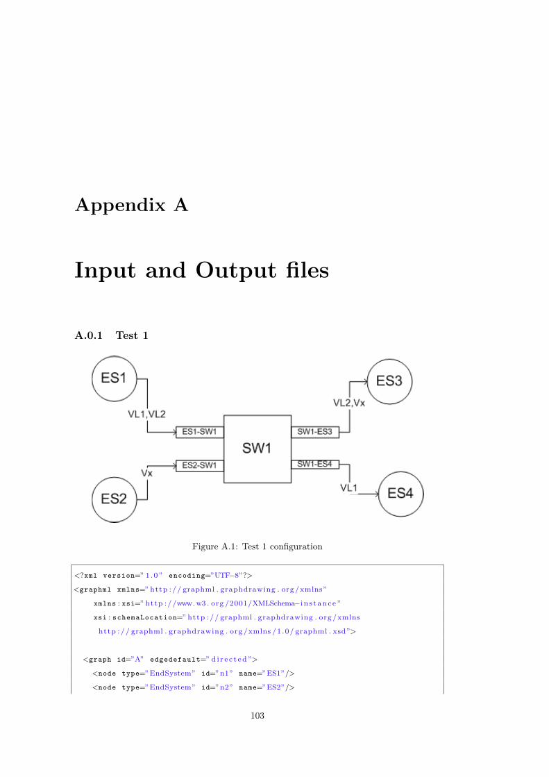
Appendix A
Input and Output files
A.0.1 Test 1
Figure A.1: Test 1 configuration
<?xml version=” 1 .0 ” encoding=”UTF−8”?>
<graphml xmlns=” http :// graphml . graphdrawing . org /xmlns”
xmlns : xsi=” http ://www. w3 . org /2001/XMLSchema−i n s t ance ”
xsi : schemaLocation=” http :// graphml . graphdrawing . org /xmlns
http :// graphml . graphdrawing . org /xmlns /1 .0/ graphml . xsd”>
<graph id=”A” edgedefault=” d i r e c t e d ”>
<node type=”EndSystem” id=”n1” name=”ES1”/>
<node type=”EndSystem” id=”n2” name=”ES2”/>
103
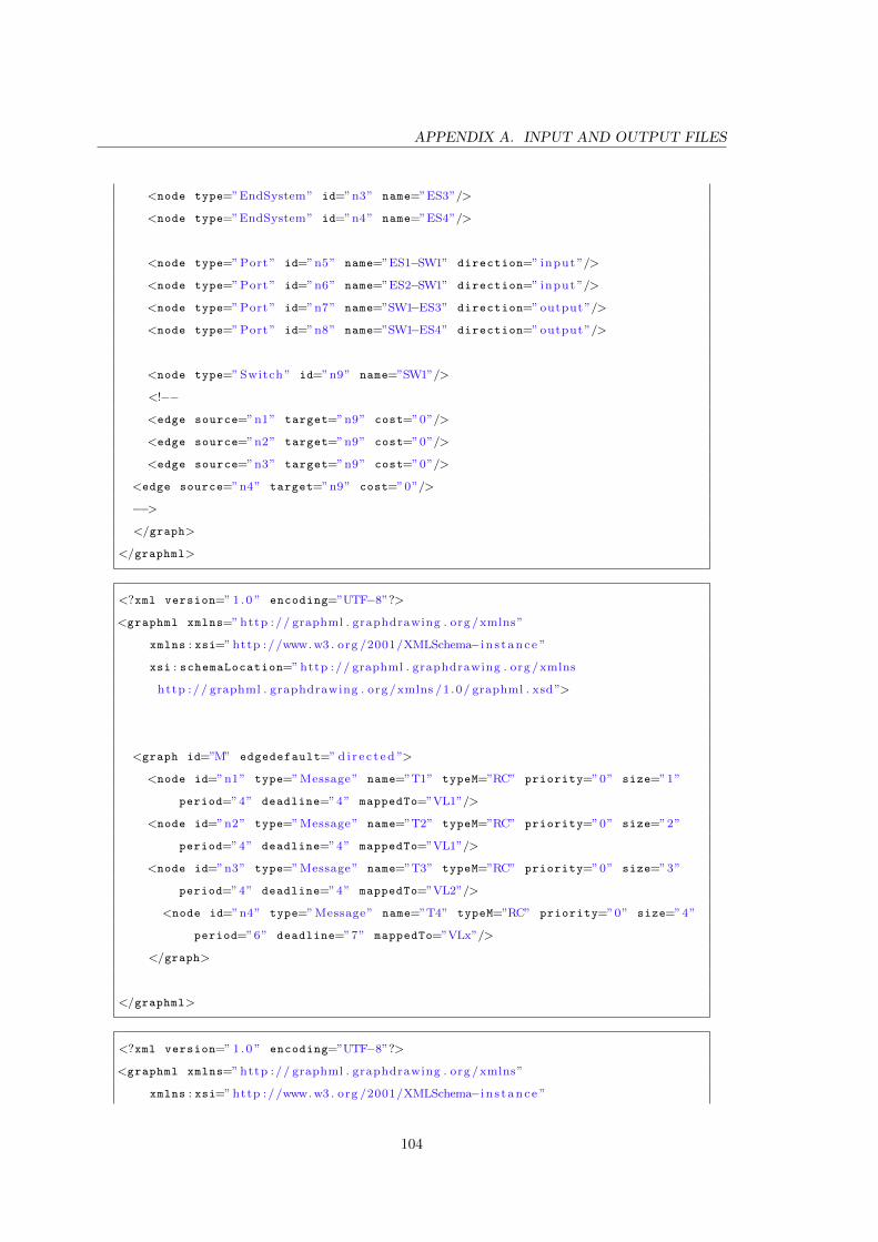
APPENDIX A. INPUT AND OUTPUT FILES
<node type=”EndSystem” id=”n3” name=”ES3”/>
<node type=”EndSystem” id=”n4” name=”ES4”/>
<node type=”Port” id=”n5” name=”ES1−SW1” direction=” input ”/>
<node type=”Port” id=”n6” name=”ES2−SW1” direction=” input ”/>
<node type=”Port” id=”n7” name=”SW1−ES3” direction=” output ”/>
<node type=”Port” id=”n8” name=”SW1−ES4” direction=” output ”/>
<node type=” Switch ” id=”n9” name=”SW1”/>
<!−−
<edge source=”n1” target=”n9” cost=”0”/>
<edge source=”n2” target=”n9” cost=”0”/>
<edge source=”n3” target=”n9” cost=”0”/>
<edge source=”n4” target=”n9” cost=”0”/>
−−>
</graph>
</graphml>
<?xml version=” 1 .0 ” encoding=”UTF−8”?>
<graphml xmlns=” http :// graphml . graphdrawing . org /xmlns”
xmlns : xsi=” http ://www. w3 . org /2001/XMLSchema−i n s t ance ”
xsi : schemaLocation=” http :// graphml . graphdrawing . org /xmlns
http :// graphml . graphdrawing . org /xmlns /1 .0/ graphml . xsd”>
<graph id=”M” edgedefault=” d i r e c t e d ”>
<node id=”n1” type=”Message” name=”T1” typeM=”RC” priority=”0” size=”1”
period=”4” deadline=”4” mappedTo=”VL1”/>
<node id=”n2” type=”Message” name=”T2” typeM=”RC” priority=”0” size=”2”
period=”4” deadline=”4” mappedTo=”VL1”/>
<node id=”n3” type=”Message” name=”T3” typeM=”RC” priority=”0” size=”3”
period=”4” deadline=”4” mappedTo=”VL2”/>
<node id=”n4” type=”Message” name=”T4” typeM=”RC” priority=”0” size=”4”
period=”6” deadline=”7” mappedTo=”VLx”/>
</graph>
</graphml>
<?xml version=” 1 .0 ” encoding=”UTF−8”?>
<graphml xmlns=” http :// graphml . graphdrawing . org /xmlns”
xmlns : xsi=” http ://www. w3 . org /2001/XMLSchema−i n s t ance ”
104
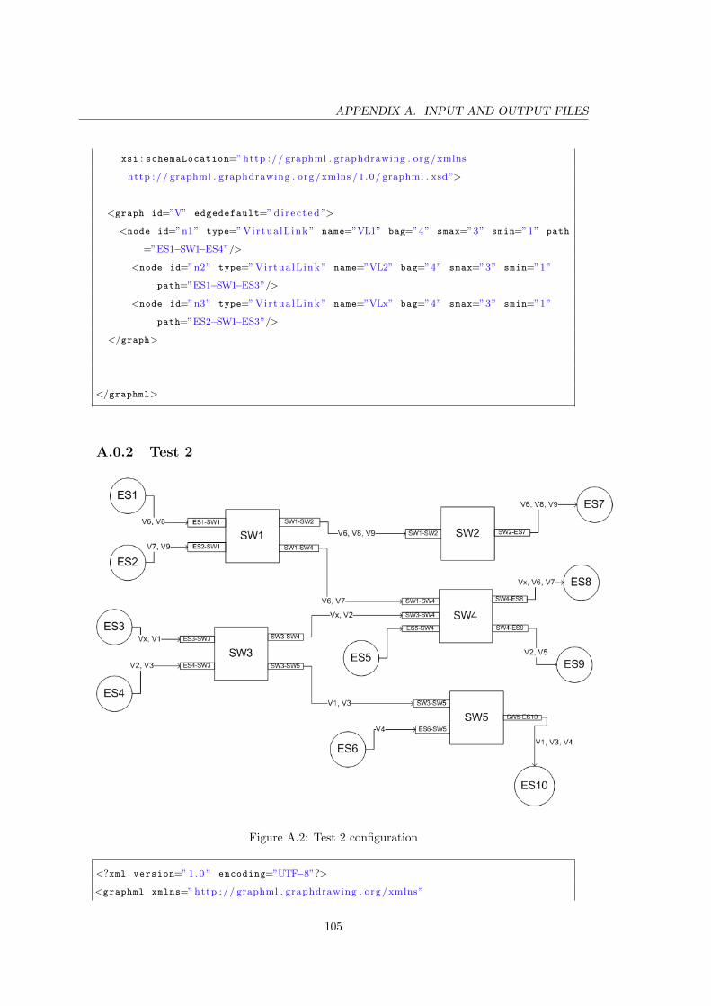
APPENDIX A. INPUT AND OUTPUT FILES
xsi : schemaLocation=” http :// graphml . graphdrawing . org /xmlns
http :// graphml . graphdrawing . org /xmlns /1 .0/ graphml . xsd”>
<graph id=”V” edgedefault=” d i r e c t e d ”>
<node id=”n1” type=” Virtua lL ink ” name=”VL1” bag=”4” smax=”3” smin=”1” path
=”ES1−SW1−ES4”/>
<node id=”n2” type=” Virtua lL ink ” name=”VL2” bag=”4” smax=”3” smin=”1”
path=”ES1−SW1−ES3”/>
<node id=”n3” type=” Virtua lL ink ” name=”VLx” bag=”4” smax=”3” smin=”1”
path=”ES2−SW1−ES3”/>
</graph>
</graphml>
A.0.2 Test 2
Figure A.2: Test 2 configuration
<?xml version=” 1 .0 ” encoding=”UTF−8”?>
<graphml xmlns=” http :// graphml . graphdrawing . org /xmlns”
105
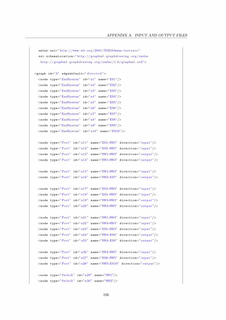
APPENDIX A. INPUT AND OUTPUT FILES
xmlns : xsi=” http ://www. w3 . org /2001/XMLSchema−i n s t ance ”
xsi : schemaLocation=” http :// graphml . graphdrawing . org /xmlns
http :// graphml . graphdrawing . org /xmlns /1 .0/ graphml . xsd”>
<graph id=”A” edgedefault=” d i r e c t e d ”>
<node type=”EndSystem” id=”n1” name=”ES1”/>
<node type=”EndSystem” id=”n2” name=”ES2”/>
<node type=”EndSystem” id=”n3” name=”ES3”/>
<node type=”EndSystem” id=”n4” name=”ES4”/>
<node type=”EndSystem” id=”n5” name=”ES5”/>
<node type=”EndSystem” id=”n6” name=”ES6”/>
<node type=”EndSystem” id=”n7” name=”ES7”/>
<node type=”EndSystem” id=”n8” name=”ES8”/>
<node type=”EndSystem” id=”n9” name=”ES9”/>
<node type=”EndSystem” id=”n10” name=”ES10”/>
<node type=”Port” id=”n11” name=”ES1−SW1” direction=” input ”/>
<node type=”Port” id=”n12” name=”ES2−SW1” direction=” input ”/>
<node type=”Port” id=”n13” name=”SW1−SW2” direction=” output ”/>
<node type=”Port” id=”n14” name=”SW1−SW4” direction=” output ”/>
<node type=”Port” id=”n15” name=”SW1−SW2” direction=” input ”/>
<node type=”Port” id=”n16” name=”SW2−ES7” direction=” output ”/>
<node type=”Port” id=”n17” name=”ES3−SW3” direction=” input ”/>
<node type=”Port” id=”n18” name=”ES4−SW3” direction=” input ”/>
<node type=”Port” id=”n19” name=”SW3−SW4” direction=” output ”/>
<node type=”Port” id=”n20” name=”SW3−SW5” direction=” output ”/>
<node type=”Port” id=”n21” name=”SW1−SW4” direction=” input ”/>
<node type=”Port” id=”n22” name=”SW3−SW4” direction=” input ”/>
<node type=”Port” id=”n23” name=”ES5−SW4” direction=” input ”/>
<node type=”Port” id=”n24” name=”SW4−ES8” direction=” output ”/>
<node type=”Port” id=”n25” name=”SW4−ES9” direction=” output ”/>
<node type=”Port” id=”n26” name=”SW3−SW5” direction=” input ”/>
<node type=”Port” id=”n27” name=”ES6−SW5” direction=” input ”/>
<node type=”Port” id=”n28” name=”SW5−ES10” direction=” output ”/>
<node type=” Switch ” id=”n29” name=”SW1”/>
<node type=” Switch ” id=”n30” name=”SW2”/>
106
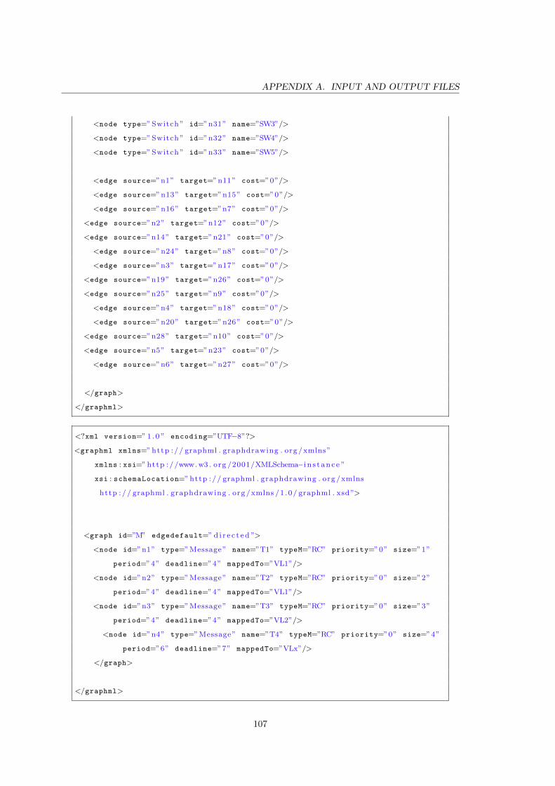
APPENDIX A. INPUT AND OUTPUT FILES
<node type=” Switch ” id=”n31” name=”SW3”/>
<node type=” Switch ” id=”n32” name=”SW4”/>
<node type=” Switch ” id=”n33” name=”SW5”/>
<edge source=”n1” target=”n11” cost=”0”/>
<edge source=”n13” target=”n15” cost=”0”/>
<edge source=”n16” target=”n7” cost=”0”/>
<edge source=”n2” target=”n12” cost=”0”/>
<edge source=”n14” target=”n21” cost=”0”/>
<edge source=”n24” target=”n8” cost=”0”/>
<edge source=”n3” target=”n17” cost=”0”/>
<edge source=”n19” target=”n26” cost=”0”/>
<edge source=”n25” target=”n9” cost=”0”/>
<edge source=”n4” target=”n18” cost=”0”/>
<edge source=”n20” target=”n26” cost=”0”/>
<edge source=”n28” target=”n10” cost=”0”/>
<edge source=”n5” target=”n23” cost=”0”/>
<edge source=”n6” target=”n27” cost=”0”/>
</graph>
</graphml>
<?xml version=” 1 .0 ” encoding=”UTF−8”?>
<graphml xmlns=” http :// graphml . graphdrawing . org /xmlns”
xmlns : xsi=” http ://www. w3 . org /2001/XMLSchema−i n s t ance ”
xsi : schemaLocation=” http :// graphml . graphdrawing . org /xmlns
http :// graphml . graphdrawing . org /xmlns /1 .0/ graphml . xsd”>
<graph id=”M” edgedefault=” d i r e c t e d ”>
<node id=”n1” type=”Message” name=”T1” typeM=”RC” priority=”0” size=”1”
period=”4” deadline=”4” mappedTo=”VL1”/>
<node id=”n2” type=”Message” name=”T2” typeM=”RC” priority=”0” size=”2”
period=”4” deadline=”4” mappedTo=”VL1”/>
<node id=”n3” type=”Message” name=”T3” typeM=”RC” priority=”0” size=”3”
period=”4” deadline=”4” mappedTo=”VL2”/>
<node id=”n4” type=”Message” name=”T4” typeM=”RC” priority=”0” size=”4”
period=”6” deadline=”7” mappedTo=”VLx”/>
</graph>
</graphml>
107
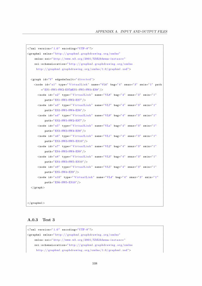
APPENDIX A. INPUT AND OUTPUT FILES
<?xml version=” 1 .0 ” encoding=”UTF−8”?>
<graphml xmlns=” http :// graphml . graphdrawing . org /xmlns”
xmlns : xsi=” http ://www. w3 . org /2001/XMLSchema−i n s t ance ”
xsi : schemaLocation=” http :// graphml . graphdrawing . org /xmlns
http :// graphml . graphdrawing . org /xmlns /1 .0/ graphml . xsd”>
<graph id=”V” edgedefault=” d i r e c t e d ”>
<node id=”n1” type=” Virtua lL ink ” name=”VL6” bag=”4” smax=”3” smin=”1” path
=”ES1−SW1−SW2−ES7#ES1−SW1−SW4−ES8”/>
<node id=”n2” type=” Virtua lL ink ” name=”VL8” bag=”4” smax=”3” smin=”1”
path=”ES1−SW1−SW2−ES7”/>
<node id=”n3” type=” Virtua lL ink ” name=”VL7” bag=”4” smax=”3” smin=”1”
path=”ES2−SW1−SW4−ES8”/>
<node id=”n4” type=” Virtua lL ink ” name=”VL9” bag=”4” smax=”3” smin=”1”
path=”ES2−SW1−SW2−ES7”/>
<node id=”n5” type=” Virtua lL ink ” name=”VLx” bag=”4” smax=”3” smin=”1”
path=”ES3−SW3−SW4−ES8”/>
<node id=”n6” type=” Virtua lL ink ” name=”VL1” bag=”4” smax=”3” smin=”1”
path=”ES3−SW3−SW5−ES10”/>
<node id=”n7” type=” Virtua lL ink ” name=”VL2” bag=”4” smax=”3” smin=”1”
path=”ES4−SW3−SW4−ES9”/>
<node id=”n8” type=” Virtua lL ink ” name=”VL3” bag=”4” smax=”3” smin=”1”
path=”ES4−SW3−SW5−ES10”/>
<node id=”n9” type=” Virtua lL ink ” name=”VL5” bag=”4” smax=”3” smin=”1”
path=”ES5−SW4−ES9”/>
<node id=”n10” type=” Virtua lL ink ” name=”VL4” bag=”4” smax=”3” smin=”1”
path=”ES6−SW5−ES10”/>
</graph>
</graphml>
A.0.3 Test 3
<?xml version=” 1 .0 ” encoding=”UTF−8”?>
<graphml xmlns=” http :// graphml . graphdrawing . org /xmlns”
xmlns : xsi=” http ://www. w3 . org /2001/XMLSchema−i n s t ance ”
xsi : schemaLocation=” http :// graphml . graphdrawing . org /xmlns
http :// graphml . graphdrawing . org /xmlns /1 .0/ graphml . xsd”>
108
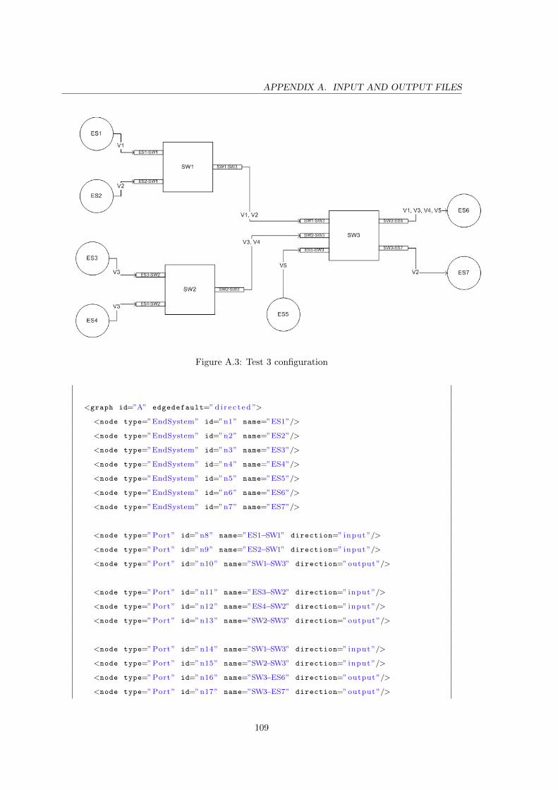
APPENDIX A. INPUT AND OUTPUT FILES
Figure A.3: Test 3 configuration
<graph id=”A” edgedefault=” d i r e c t e d ”>
<node type=”EndSystem” id=”n1” name=”ES1”/>
<node type=”EndSystem” id=”n2” name=”ES2”/>
<node type=”EndSystem” id=”n3” name=”ES3”/>
<node type=”EndSystem” id=”n4” name=”ES4”/>
<node type=”EndSystem” id=”n5” name=”ES5”/>
<node type=”EndSystem” id=”n6” name=”ES6”/>
<node type=”EndSystem” id=”n7” name=”ES7”/>
<node type=”Port” id=”n8” name=”ES1−SW1” direction=” input ”/>
<node type=”Port” id=”n9” name=”ES2−SW1” direction=” input ”/>
<node type=”Port” id=”n10” name=”SW1−SW3” direction=” output ”/>
<node type=”Port” id=”n11” name=”ES3−SW2” direction=” input ”/>
<node type=”Port” id=”n12” name=”ES4−SW2” direction=” input ”/>
<node type=”Port” id=”n13” name=”SW2−SW3” direction=” output ”/>
<node type=”Port” id=”n14” name=”SW1−SW3” direction=” input ”/>
<node type=”Port” id=”n15” name=”SW2−SW3” direction=” input ”/>
<node type=”Port” id=”n16” name=”SW3−ES6” direction=” output ”/>
<node type=”Port” id=”n17” name=”SW3−ES7” direction=” output ”/>
109
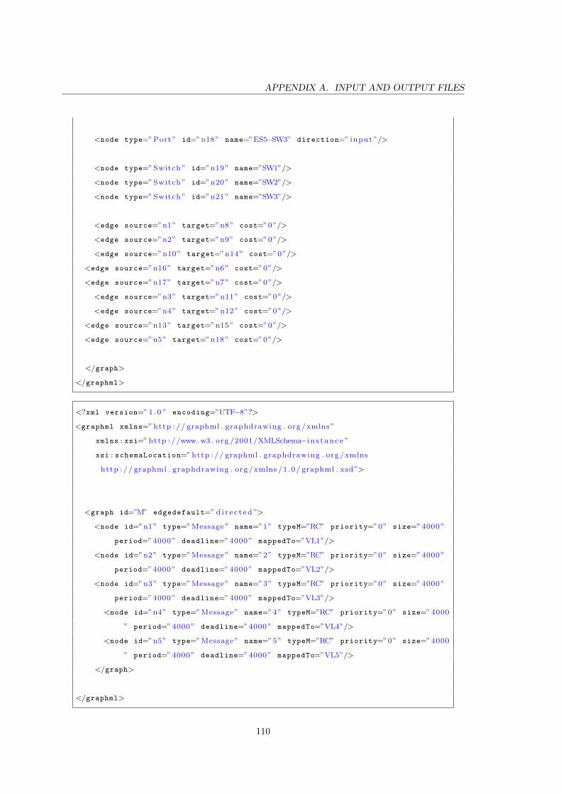
APPENDIX A. INPUT AND OUTPUT FILES
<node type=”Port” id=”n18” name=”ES5−SW3” direction=” input ”/>
<node type=” Switch ” id=”n19” name=”SW1”/>
<node type=” Switch ” id=”n20” name=”SW2”/>
<node type=” Switch ” id=”n21” name=”SW3”/>
<edge source=”n1” target=”n8” cost=”0”/>
<edge source=”n2” target=”n9” cost=”0”/>
<edge source=”n10” target=”n14” cost=”0”/>
<edge source=”n16” target=”n6” cost=”0”/>
<edge source=”n17” target=”n7” cost=”0”/>
<edge source=”n3” target=”n11” cost=”0”/>
<edge source=”n4” target=”n12” cost=”0”/>
<edge source=”n13” target=”n15” cost=”0”/>
<edge source=”n5” target=”n18” cost=”0”/>
</graph>
</graphml>
<?xml version=” 1 .0 ” encoding=”UTF−8”?>
<graphml xmlns=” http :// graphml . graphdrawing . org /xmlns”
xmlns : xsi=” http ://www. w3 . org /2001/XMLSchema−i n s t ance ”
xsi : schemaLocation=” http :// graphml . graphdrawing . org /xmlns
http :// graphml . graphdrawing . org /xmlns /1 .0/ graphml . xsd”>
<graph id=”M” edgedefault=” d i r e c t e d ”>
<node id=”n1” type=”Message” name=”1” typeM=”RC” priority=”0” size=”4000”
period=”4000” deadline=”4000” mappedTo=”VL1”/>
<node id=”n2” type=”Message” name=”2” typeM=”RC” priority=”0” size=”4000”
period=”4000” deadline=”4000” mappedTo=”VL2”/>
<node id=”n3” type=”Message” name=”3” typeM=”RC” priority=”0” size=”4000”
period=”4000” deadline=”4000” mappedTo=”VL3”/>
<node id=”n4” type=”Message” name=”4” typeM=”RC” priority=”0” size=”4000
” period=”4000” deadline=”4000” mappedTo=”VL4”/>
<node id=”n5” type=”Message” name=”5” typeM=”RC” priority=”0” size=”4000
” period=”4000” deadline=”4000” mappedTo=”VL5”/>
</graph>
</graphml>
110
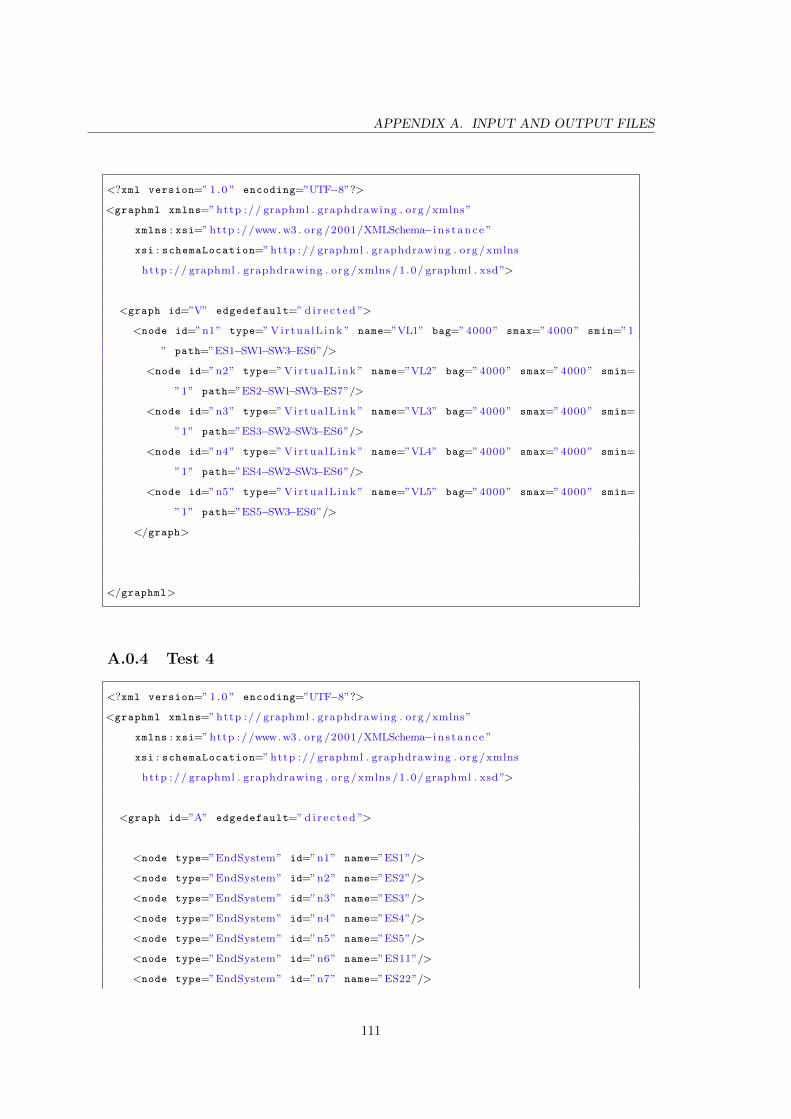
APPENDIX A. INPUT AND OUTPUT FILES
<?xml version=” 1 .0 ” encoding=”UTF−8”?>
<graphml xmlns=” http :// graphml . graphdrawing . org /xmlns”
xmlns : xsi=” http ://www. w3 . org /2001/XMLSchema−i n s t ance ”
xsi : schemaLocation=” http :// graphml . graphdrawing . org /xmlns
http :// graphml . graphdrawing . org /xmlns /1 .0/ graphml . xsd”>
<graph id=”V” edgedefault=” d i r e c t e d ”>
<node id=”n1” type=” Virtua lL ink ” name=”VL1” bag=”4000” smax=”4000” smin=”1
” path=”ES1−SW1−SW3−ES6”/>
<node id=”n2” type=” Virtua lL ink ” name=”VL2” bag=”4000” smax=”4000” smin=
”1” path=”ES2−SW1−SW3−ES7”/>
<node id=”n3” type=” Virtua lL ink ” name=”VL3” bag=”4000” smax=”4000” smin=
”1” path=”ES3−SW2−SW3−ES6”/>
<node id=”n4” type=” Virtua lL ink ” name=”VL4” bag=”4000” smax=”4000” smin=
”1” path=”ES4−SW2−SW3−ES6”/>
<node id=”n5” type=” Virtua lL ink ” name=”VL5” bag=”4000” smax=”4000” smin=
”1” path=”ES5−SW3−ES6”/>
</graph>
</graphml>
A.0.4 Test 4
<?xml version=” 1 .0 ” encoding=”UTF−8”?>
<graphml xmlns=” http :// graphml . graphdrawing . org /xmlns”
xmlns : xsi=” http ://www. w3 . org /2001/XMLSchema−i n s t ance ”
xsi : schemaLocation=” http :// graphml . graphdrawing . org /xmlns
http :// graphml . graphdrawing . org /xmlns /1 .0/ graphml . xsd”>
<graph id=”A” edgedefault=” d i r e c t e d ”>
<node type=”EndSystem” id=”n1” name=”ES1”/>
<node type=”EndSystem” id=”n2” name=”ES2”/>
<node type=”EndSystem” id=”n3” name=”ES3”/>
<node type=”EndSystem” id=”n4” name=”ES4”/>
<node type=”EndSystem” id=”n5” name=”ES5”/>
<node type=”EndSystem” id=”n6” name=”ES11”/>
<node type=”EndSystem” id=”n7” name=”ES22”/>
111
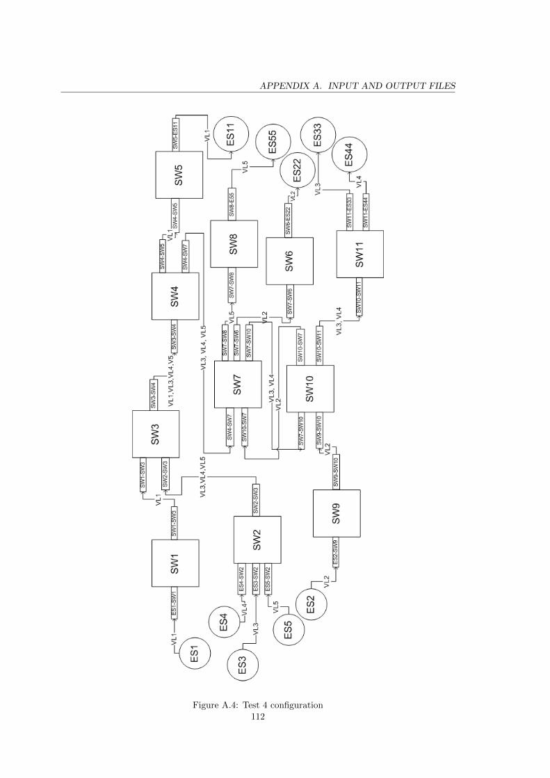
APPENDIX A. INPUT AND OUTPUT FILES
Figure A.4: Test 4 configuration112
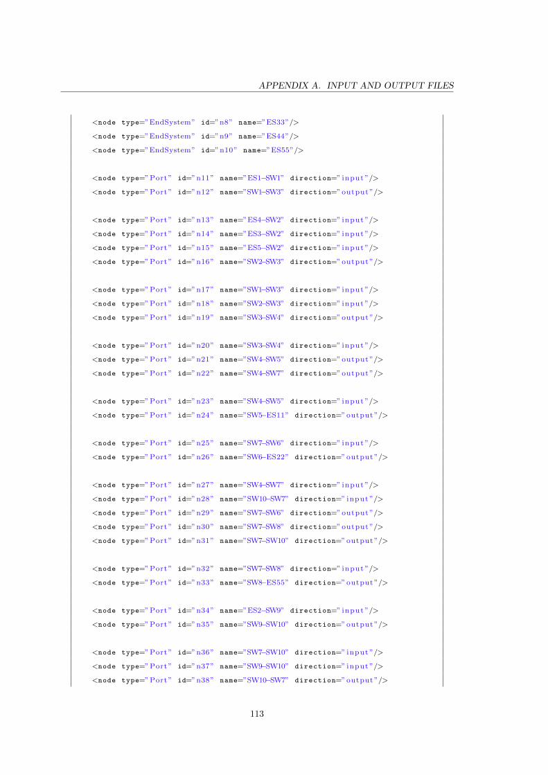
APPENDIX A. INPUT AND OUTPUT FILES
<node type=”EndSystem” id=”n8” name=”ES33”/>
<node type=”EndSystem” id=”n9” name=”ES44”/>
<node type=”EndSystem” id=”n10” name=”ES55”/>
<node type=”Port” id=”n11” name=”ES1−SW1” direction=” input ”/>
<node type=”Port” id=”n12” name=”SW1−SW3” direction=” output ”/>
<node type=”Port” id=”n13” name=”ES4−SW2” direction=” input ”/>
<node type=”Port” id=”n14” name=”ES3−SW2” direction=” input ”/>
<node type=”Port” id=”n15” name=”ES5−SW2” direction=” input ”/>
<node type=”Port” id=”n16” name=”SW2−SW3” direction=” output ”/>
<node type=”Port” id=”n17” name=”SW1−SW3” direction=” input ”/>
<node type=”Port” id=”n18” name=”SW2−SW3” direction=” input ”/>
<node type=”Port” id=”n19” name=”SW3−SW4” direction=” output ”/>
<node type=”Port” id=”n20” name=”SW3−SW4” direction=” input ”/>
<node type=”Port” id=”n21” name=”SW4−SW5” direction=” output ”/>
<node type=”Port” id=”n22” name=”SW4−SW7” direction=” output ”/>
<node type=”Port” id=”n23” name=”SW4−SW5” direction=” input ”/>
<node type=”Port” id=”n24” name=”SW5−ES11” direction=” output ”/>
<node type=”Port” id=”n25” name=”SW7−SW6” direction=” input ”/>
<node type=”Port” id=”n26” name=”SW6−ES22” direction=” output ”/>
<node type=”Port” id=”n27” name=”SW4−SW7” direction=” input ”/>
<node type=”Port” id=”n28” name=”SW10−SW7” direction=” input ”/>
<node type=”Port” id=”n29” name=”SW7−SW6” direction=” output ”/>
<node type=”Port” id=”n30” name=”SW7−SW8” direction=” output ”/>
<node type=”Port” id=”n31” name=”SW7−SW10” direction=” output ”/>
<node type=”Port” id=”n32” name=”SW7−SW8” direction=” input ”/>
<node type=”Port” id=”n33” name=”SW8−ES55” direction=” output ”/>
<node type=”Port” id=”n34” name=”ES2−SW9” direction=” input ”/>
<node type=”Port” id=”n35” name=”SW9−SW10” direction=” output ”/>
<node type=”Port” id=”n36” name=”SW7−SW10” direction=” input ”/>
<node type=”Port” id=”n37” name=”SW9−SW10” direction=” input ”/>
<node type=”Port” id=”n38” name=”SW10−SW7” direction=” output ”/>
113
APPENDIX A. INPUT AND OUTPUT FILES
<node type=”Port” id=”n39” name=”SW10−SW11” direction=” output ”/>
<node type=”Port” id=”n40” name=”SW10−SW11” direction=” input ”/>
<node type=”Port” id=”n41” name=”SW11−ES33” direction=” output ”/>
<node type=”Port” id=”n42” name=”SW11−ES44” direction=” output ”/>
<node type=” Switch ” id=”n43” name=”SW1”/>
<node type=” Switch ” id=”n44” name=”SW2”/>
<node type=” Switch ” id=”n45” name=”SW3”/>
<node type=” Switch ” id=”n46” name=”SW4”/>
<node type=” Switch ” id=”n47” name=”SW5”/>
<node type=” Switch ” id=”n48” name=”SW6”/>
<node type=” Switch ” id=”n49” name=”SW7”/>
<node type=” Switch ” id=”n50” name=”SW8”/>
<node type=” Switch ” id=”n51” name=”SW9”/>
<node type=” Switch ” id=”n52” name=”SW10”/>
<node type=” Switch ” id=”n53” name=”SW11”/>
</graph>
</graphml>
<?xml version=” 1 .0 ” encoding=”UTF−8”?>
<graphml xmlns=” http :// graphml . graphdrawing . org /xmlns”
xmlns : xsi=” http ://www. w3 . org /2001/XMLSchema−i n s t ance ”
xsi : schemaLocation=” http :// graphml . graphdrawing . org /xmlns
http :// graphml . graphdrawing . org /xmlns /1 .0/ graphml . xsd”>
<graph id=”M” edgedefault=” d i r e c t e d ”>
<node id=”n1” type=”Message” name=”1” typeM=”RC” priority=”0” size=”400”
period=”36” deadline=”3600” mappedTo=”VL1”/>
<node id=”n2” type=”Message” name=”2” typeM=”RC” priority=”0” size=”400”
period=”36” deadline=”3600” mappedTo=”VL2”/>
<node id=”n3” type=”Message” name=”3” typeM=”RC” priority=”0” size=”400”
period=”36” deadline=”3600” mappedTo=”VL3”/>
<node id=”n4” type=”Message” name=”4” typeM=”RC” priority=”0” size=”400”
period=”36” deadline=”3600” mappedTo=”VL4”/>
<node id=”n5” type=”Message” name=”5” typeM=”RC” priority=”0” size=”400”
period=”36” deadline=”3600” mappedTo=”VL5”/>
</graph>
114
APPENDIX A. INPUT AND OUTPUT FILES
</graphml>
<?xml version=” 1 .0 ” encoding=”UTF−8”?>
<graphml xmlns=” http :// graphml . graphdrawing . org /xmlns”
xmlns : xsi=” http ://www. w3 . org /2001/XMLSchema−i n s t ance ”
xsi : schemaLocation=” http :// graphml . graphdrawing . org /xmlns
http :// graphml . graphdrawing . org /xmlns /1 .0/ graphml . xsd”>
<graph id=”V” edgedefault=” d i r e c t e d ”>
<node id=”n1” type=” Virtua lL ink ” name=”VL1” bag=”36” smax=”400” smin=”1”
path=”ES1−SW1−SW3−SW4−SW5−ES11”/>
<node id=”n2” type=” Virtua lL ink ” name=”VL2” bag=”36” smax=”400” smin=”1”
path=”ES2−SW9−SW10−SW7−SW6−ES22”/>
<node id=”n3” type=” Virtua lL ink ” name=”VL3” bag=”36” smax=”400” smin=”1”
path=”ES3−SW2−SW3−SW4−SW7−SW10−SW11−ES33”/>
<node id=”n4” type=” Virtua lL ink ” name=”VL4” bag=”36” smax=”400” smin=”1”
path=”ES4−SW2−SW3−SW4−SW7−SW10−SW11−ES44”/>
<node id=”n5” type=” Virtua lL ink ” name=”VL5” bag=”36” smax=”400” smin=”1”
path=”ES5−SW2−SW3−SW4−SW7−SW8−ES55”/>
</graph>
</graphml>
A.0.5 Test 5
<?xml version=” 1 .0 ” encoding=”UTF−8”?>
<graphml xmlns=” http :// graphml . graphdrawing . org /xmlns”
xmlns : xsi=” http ://www. w3 . org /2001/XMLSchema−i n s t ance ”
xsi : schemaLocation=” http :// graphml . graphdrawing . org /xmlns
http :// graphml . graphdrawing . org /xmlns /1 .0/ graphml . xsd”>
<graph id=”A” edgedefault=” d i r e c t e d ”>
<node type=”EndSystem” id=”n1” name=”ES1”/>
<node type=”EndSystem” id=”n2” name=”ES2”/>
<node type=”EndSystem” id=”n3” name=”ES3”/>
<node type=”EndSystem” id=”n4” name=”ES4”/>
<node type=”EndSystem” id=”n5” name=”ES5”/>
<node type=”Port” id=”n6” name=”ES1−SW1” direction=” input ”/>
115
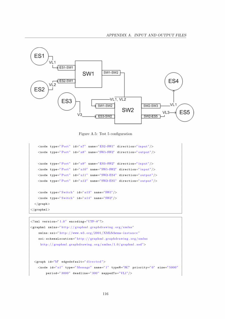
APPENDIX A. INPUT AND OUTPUT FILES
Figure A.5: Test 5 configuration
<node type=”Port” id=”n7” name=”ES2−SW1” direction=” input ”/>
<node type=”Port” id=”n8” name=”SW1−SW2” direction=” output ”/>
<node type=”Port” id=”n9” name=”ES3−SW2” direction=” input ”/>
<node type=”Port” id=”n10” name=”SW1−SW2” direction=” input ”/>
<node type=”Port” id=”n11” name=”SW2−ES4” direction=” output ”/>
<node type=”Port” id=”n12” name=”SW2−ES5” direction=” output ”/>
<node type=” Switch ” id=”n13” name=”SW1”/>
<node type=” Switch ” id=”n14” name=”SW2”/>
</graph>
</graphml>
<?xml version=” 1 .0 ” encoding=”UTF−8”?>
<graphml xmlns=” http :// graphml . graphdrawing . org /xmlns”
xmlns : xsi=” http ://www. w3 . org /2001/XMLSchema−i n s t ance ”
xsi : schemaLocation=” http :// graphml . graphdrawing . org /xmlns
http :// graphml . graphdrawing . org /xmlns /1 .0/ graphml . xsd”>
<graph id=”M” edgedefault=” d i r e c t e d ”>
<node id=”n1” type=”Message” name=”1” typeM=”RC” priority=”0” size=”5000”
period=”3000” deadline=”300” mappedTo=”VL1”/>
116
APPENDIX A. INPUT AND OUTPUT FILES
<node id=”n2” type=”Message” name=”2” typeM=”RC” priority=”0” size=”5000”
period=”3000” deadline=”300” mappedTo=”VL2”/>
<node id=”n3” type=”Message” name=”3” typeM=”RC” priority=”0” size=”5000”
period=”3000” deadline=”300” mappedTo=”VL3”/>
</graph>
</graphml>
<?xml version=” 1 .0 ” encoding=”UTF−8”?>
<graphml xmlns=” http :// graphml . graphdrawing . org /xmlns”
xmlns : xsi=” http ://www. w3 . org /2001/XMLSchema−i n s t ance ”
xsi : schemaLocation=” http :// graphml . graphdrawing . org /xmlns
http :// graphml . graphdrawing . org /xmlns /1 .0/ graphml . xsd”>
<graph id=”V” edgedefault=” d i r e c t e d ”>
<node id=”n1” type=” Virtua lL ink ” name=”VL1” bag=”3000” smax=”5000” smin=”
5000” path=”ES1−SW1−SW2−ES4”/>
<node id=”n2” type=” Virtua lL ink ” name=”VL2” bag=”300” smax=”5000” smin=”
5000” path=”ES2−SW1−SW2−ES5”/>
<node id=”n3” type=” Virtua lL ink ” name=”VL3” bag=”3000” smax=”5000” smin=
”5000” path=”ES3−SW2−ES4”/>
</graph>
</graphml>
A.0.6 Test 6
<?xml version=” 1 .0 ” encoding=”UTF−8”?>
<graphml xmlns=” http :// graphml . graphdrawing . org /xmlns”
xmlns : xsi=” http ://www. w3 . org /2001/XMLSchema−i n s t ance ”
xsi : schemaLocation=” http :// graphml . graphdrawing . org /xmlns
http :// graphml . graphdrawing . org /xmlns /1 .0/ graphml . xsd”>
<graph id=”A” edgedefault=” d i r e c t e d ”>
<node type=”EndSystem” id=”n1” name=”ES1”/>
<node type=”EndSystem” id=”n2” name=”ES2”/>
<node type=”EndSystem” id=”n3” name=”ES3”/>
<node type=”EndSystem” id=”n4” name=”ES11”/>
<node type=”EndSystem” id=”n5” name=”ES22”/>
117
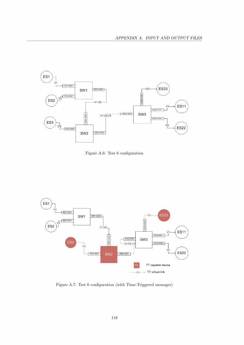
APPENDIX A. INPUT AND OUTPUT FILES
Figure A.6: Test 6 configuration
Figure A.7: Test 6 configuration (with Time-Triggered messages)
118
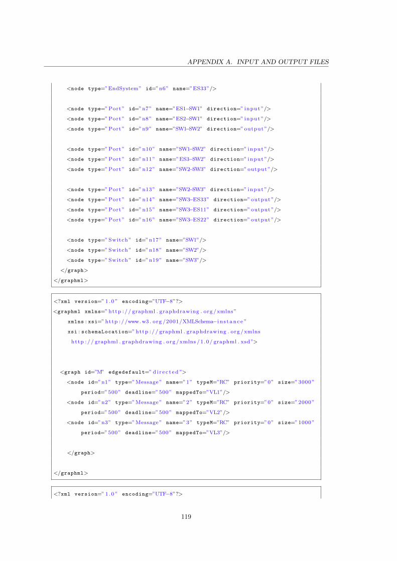
APPENDIX A. INPUT AND OUTPUT FILES
<node type=”EndSystem” id=”n6” name=”ES33”/>
<node type=”Port” id=”n7” name=”ES1−SW1” direction=” input ”/>
<node type=”Port” id=”n8” name=”ES2−SW1” direction=” input ”/>
<node type=”Port” id=”n9” name=”SW1−SW2” direction=” output ”/>
<node type=”Port” id=”n10” name=”SW1−SW2” direction=” input ”/>
<node type=”Port” id=”n11” name=”ES3−SW2” direction=” input ”/>
<node type=”Port” id=”n12” name=”SW2−SW3” direction=” output ”/>
<node type=”Port” id=”n13” name=”SW2−SW3” direction=” input ”/>
<node type=”Port” id=”n14” name=”SW3−ES33” direction=” output ”/>
<node type=”Port” id=”n15” name=”SW3−ES11” direction=” output ”/>
<node type=”Port” id=”n16” name=”SW3−ES22” direction=” output ”/>
<node type=” Switch ” id=”n17” name=”SW1”/>
<node type=” Switch ” id=”n18” name=”SW2”/>
<node type=” Switch ” id=”n19” name=”SW3”/>
</graph>
</graphml>
<?xml version=” 1 .0 ” encoding=”UTF−8”?>
<graphml xmlns=” http :// graphml . graphdrawing . org /xmlns”
xmlns : xsi=” http ://www. w3 . org /2001/XMLSchema−i n s t ance ”
xsi : schemaLocation=” http :// graphml . graphdrawing . org /xmlns
http :// graphml . graphdrawing . org /xmlns /1 .0/ graphml . xsd”>
<graph id=”M” edgedefault=” d i r e c t e d ”>
<node id=”n1” type=”Message” name=”1” typeM=”RC” priority=”0” size=”3000”
period=”500” deadline=”500” mappedTo=”VL1”/>
<node id=”n2” type=”Message” name=”2” typeM=”RC” priority=”0” size=”2000”
period=”500” deadline=”500” mappedTo=”VL2”/>
<node id=”n3” type=”Message” name=”3” typeM=”RC” priority=”0” size=”1000”
period=”500” deadline=”500” mappedTo=”VL3”/>
</graph>
</graphml>
<?xml version=” 1 .0 ” encoding=”UTF−8”?>
119
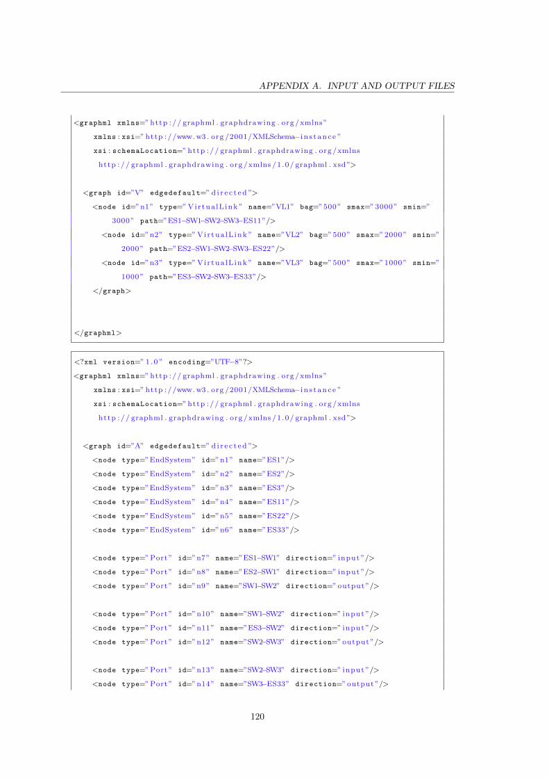
APPENDIX A. INPUT AND OUTPUT FILES
<graphml xmlns=” http :// graphml . graphdrawing . org /xmlns”
xmlns : xsi=” http ://www. w3 . org /2001/XMLSchema−i n s t ance ”
xsi : schemaLocation=” http :// graphml . graphdrawing . org /xmlns
http :// graphml . graphdrawing . org /xmlns /1 .0/ graphml . xsd”>
<graph id=”V” edgedefault=” d i r e c t e d ”>
<node id=”n1” type=” Virtua lL ink ” name=”VL1” bag=”500” smax=”3000” smin=”
3000” path=”ES1−SW1−SW2−SW3−ES11”/>
<node id=”n2” type=” Virtua lL ink ” name=”VL2” bag=”500” smax=”2000” smin=”
2000” path=”ES2−SW1−SW2−SW3−ES22”/>
<node id=”n3” type=” Virtua lL ink ” name=”VL3” bag=”500” smax=”1000” smin=”
1000” path=”ES3−SW2−SW3−ES33”/>
</graph>
</graphml>
<?xml version=” 1 .0 ” encoding=”UTF−8”?>
<graphml xmlns=” http :// graphml . graphdrawing . org /xmlns”
xmlns : xsi=” http ://www. w3 . org /2001/XMLSchema−i n s t ance ”
xsi : schemaLocation=” http :// graphml . graphdrawing . org /xmlns
http :// graphml . graphdrawing . org /xmlns /1 .0/ graphml . xsd”>
<graph id=”A” edgedefault=” d i r e c t e d ”>
<node type=”EndSystem” id=”n1” name=”ES1”/>
<node type=”EndSystem” id=”n2” name=”ES2”/>
<node type=”EndSystem” id=”n3” name=”ES3”/>
<node type=”EndSystem” id=”n4” name=”ES11”/>
<node type=”EndSystem” id=”n5” name=”ES22”/>
<node type=”EndSystem” id=”n6” name=”ES33”/>
<node type=”Port” id=”n7” name=”ES1−SW1” direction=” input ”/>
<node type=”Port” id=”n8” name=”ES2−SW1” direction=” input ”/>
<node type=”Port” id=”n9” name=”SW1−SW2” direction=” output ”/>
<node type=”Port” id=”n10” name=”SW1−SW2” direction=” input ”/>
<node type=”Port” id=”n11” name=”ES3−SW2” direction=” input ”/>
<node type=”Port” id=”n12” name=”SW2−SW3” direction=” output ”/>
<node type=”Port” id=”n13” name=”SW2−SW3” direction=” input ”/>
<node type=”Port” id=”n14” name=”SW3−ES33” direction=” output ”/>
120
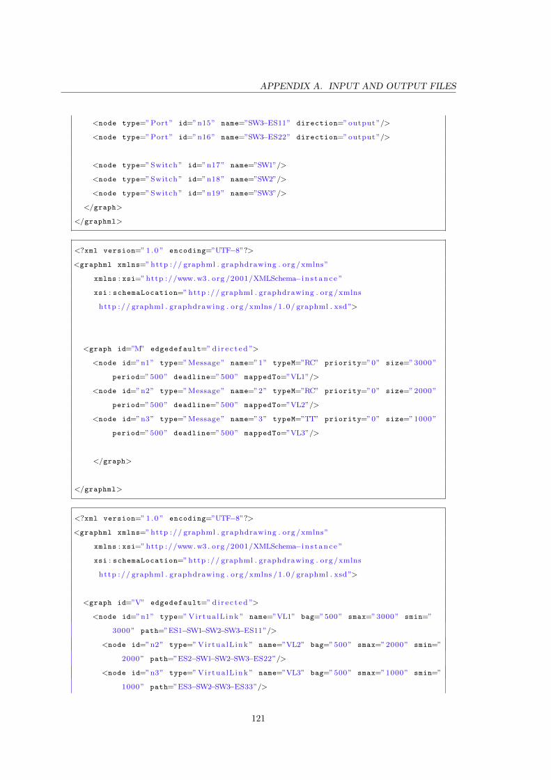
APPENDIX A. INPUT AND OUTPUT FILES
<node type=”Port” id=”n15” name=”SW3−ES11” direction=” output ”/>
<node type=”Port” id=”n16” name=”SW3−ES22” direction=” output ”/>
<node type=” Switch ” id=”n17” name=”SW1”/>
<node type=” Switch ” id=”n18” name=”SW2”/>
<node type=” Switch ” id=”n19” name=”SW3”/>
</graph>
</graphml>
<?xml version=” 1 .0 ” encoding=”UTF−8”?>
<graphml xmlns=” http :// graphml . graphdrawing . org /xmlns”
xmlns : xsi=” http ://www. w3 . org /2001/XMLSchema−i n s t ance ”
xsi : schemaLocation=” http :// graphml . graphdrawing . org /xmlns
http :// graphml . graphdrawing . org /xmlns /1 .0/ graphml . xsd”>
<graph id=”M” edgedefault=” d i r e c t e d ”>
<node id=”n1” type=”Message” name=”1” typeM=”RC” priority=”0” size=”3000”
period=”500” deadline=”500” mappedTo=”VL1”/>
<node id=”n2” type=”Message” name=”2” typeM=”RC” priority=”0” size=”2000”
period=”500” deadline=”500” mappedTo=”VL2”/>
<node id=”n3” type=”Message” name=”3” typeM=”TT” priority=”0” size=”1000”
period=”500” deadline=”500” mappedTo=”VL3”/>
</graph>
</graphml>
<?xml version=” 1 .0 ” encoding=”UTF−8”?>
<graphml xmlns=” http :// graphml . graphdrawing . org /xmlns”
xmlns : xsi=” http ://www. w3 . org /2001/XMLSchema−i n s t ance ”
xsi : schemaLocation=” http :// graphml . graphdrawing . org /xmlns
http :// graphml . graphdrawing . org /xmlns /1 .0/ graphml . xsd”>
<graph id=”V” edgedefault=” d i r e c t e d ”>
<node id=”n1” type=” Virtua lL ink ” name=”VL1” bag=”500” smax=”3000” smin=”
3000” path=”ES1−SW1−SW2−SW3−ES11”/>
<node id=”n2” type=” Virtua lL ink ” name=”VL2” bag=”500” smax=”2000” smin=”
2000” path=”ES2−SW1−SW2−SW3−ES22”/>
<node id=”n3” type=” Virtua lL ink ” name=”VL3” bag=”500” smax=”1000” smin=”
1000” path=”ES3−SW2−SW3−ES33”/>
121
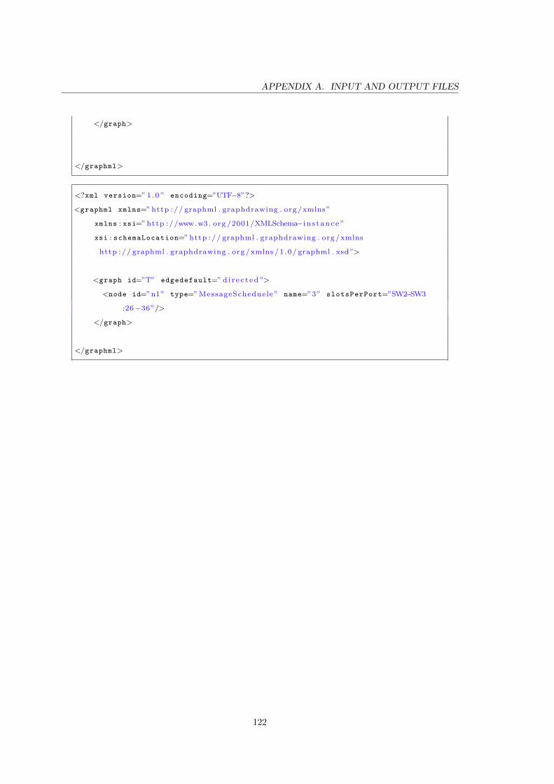
APPENDIX A. INPUT AND OUTPUT FILES
</graph>
</graphml>
<?xml version=” 1 .0 ” encoding=”UTF−8”?>
<graphml xmlns=” http :// graphml . graphdrawing . org /xmlns”
xmlns : xsi=” http ://www. w3 . org /2001/XMLSchema−i n s t ance ”
xsi : schemaLocation=” http :// graphml . graphdrawing . org /xmlns
http :// graphml . graphdrawing . org /xmlns /1 .0/ graphml . xsd”>
<graph id=”T” edgedefault=” d i r e c t e d ”>
<node id=”n1” type=” MessageScheduele ” name=”3” slotsPerPort=”SW2−SW3
:26−36”/>
</graph>
</graphml>
122


![Post Master [dpea] - WordPress.com · imm 11 imm 12 imm 13 imm 14 imm 15 posters prejury posters imm 17 imm 18 imm 19 imm 20 imm 21 imm 22 imm 23 imm 24 9h30 - 12h30 imm 16 14h30](https://img.pdfslide.net/doc/110x75/5f0c7d177e708231d435a7ad/post-master-dpea-imm-11-imm-12-imm-13-imm-14-imm-15-posters-prejury-posters.jpg)