DUAL EXTENDED KALMAN FILTER METHODS - pudn.comread.pudn.com/downloads142/ebook/620455/Kalman... · Kalman Filtering and Neural Networks, Edited by Simon Haykin ISBN 0-471-36998-5

5

DUAL EXTENDED KALMANFILTER METHODS

Eric A. Wan and Alex T. NelsonDepartment of Electrical and Computer Engineering, Oregon Graduate Institute of

Science and Technology, Beaverton, Oregon, U.S.A.

5.1 INTRODUCTION

The Extended Kalman Filter (EKF) provides an efficient method for

generating approximate maximum-likelihood estimates of the state of a

discrete-time nonlinear dynamical system (see Chapter 1). The filter

involves a recursive procedure to optimally combine noisy observations

with predictions from the known dynamic model. A second use of the

EKF involves estimating the parameters of a model (e.g., neural network)

given clean training data of input and output data (see Chapter 2). In this

case, the EKF represents a modified-Newton type of algorithm for on-line

system identification. In this chapter, we consider the dual estimation

problem, in which both the states of the dynamical system and its

parameters are estimated simultaneously, given only noisy observations.

123

Kalman Filtering and Neural Networks, Edited by Simon HaykinISBN 0-471-36998-5 # 2001 John Wiley & Sons, Inc.

Kalman Filtering and Neural Networks, Edited by Simon HaykinCopyright # 2001 John Wiley & Sons, Inc.

ISBNs: 0-471-36998-5 (Hardback); 0-471-22154-6 (Electronic)

To be more specific, we consider the problem of learning both the

hidden states xk and parameters w of a discrete-time nonlinear dynamical

system,

xkþ1 ¼ Fðxk;uk;wÞ þ vk;

yk ¼ Hðxk;wÞ þ nk;ð5:1Þ

where both the system states xk and the set of model parameters w for the

dynamical system must be simultaneously estimated from only the

observed noisy signal yk . The process noise vk drives the dynamical

system, observation noise is given by nk, and uk corresponds to observed

exogenous inputs. The model structure, Fð�Þ and Hð�Þ, may represent

multilayer neural networks, in which case w are the weights.

The problem of dual estimation can be motivated either from the need

for a model to estimate the signal or (in other applications) from the need

for good signal estimates to estimate the model. In general, applications

can be divided into the tasks of modeling, estimation, and prediction. In

estimation, all noisy data up to the current time is used to approximate the

current value of the clean state. Prediction is concerned with using all

available data to approximate a future value of the clean state. Modeling

(sometimes referred to as identification) is the process of approximating

the underlying dynamics that generated the states, again given only the

noisy observations. Specific applications may include noise reduction

(e.g., speech or image enhancement), or prediction of financial and

economic time series. Alternatively, the model may correspond to the

explicit equations derived from first principles of a robotic or vehicle

system. In this case, w corresponds to a set of unknown parameters.

Applications include adaptive control, where parameters are used in the

design process and the estimated states are used for feedback.

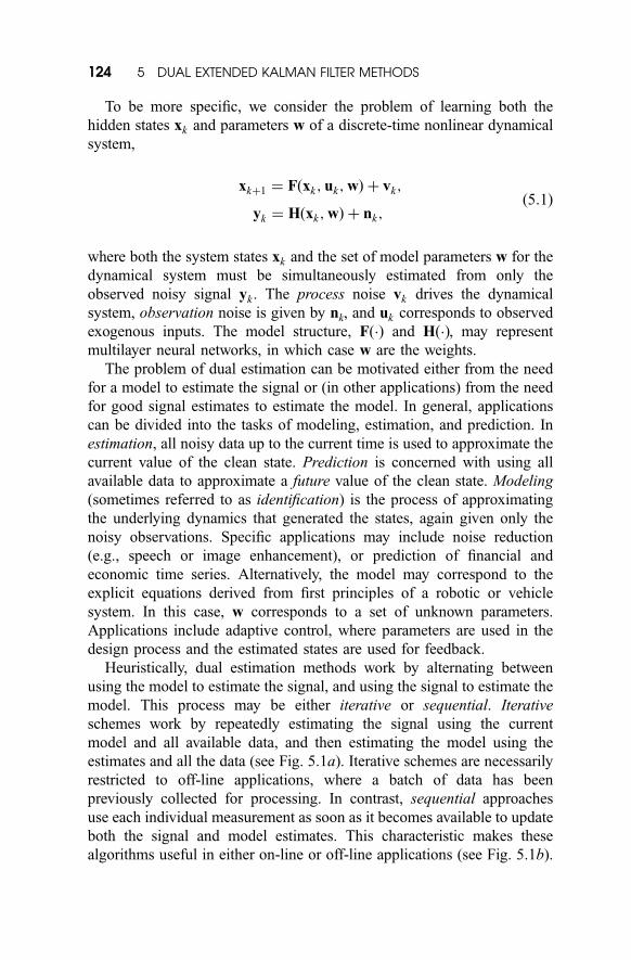
Heuristically, dual estimation methods work by alternating between

using the model to estimate the signal, and using the signal to estimate the

model. This process may be either iterative or sequential. Iterative

schemes work by repeatedly estimating the signal using the current

model and all available data, and then estimating the model using the

estimates and all the data (see Fig. 5.1a). Iterative schemes are necessarily

restricted to off-line applications, where a batch of data has been

previously collected for processing. In contrast, sequential approaches

use each individual measurement as soon as it becomes available to update

both the signal and model estimates. This characteristic makes these

algorithms useful in either on-line or off-line applications (see Fig. 5.1b).

124 5 DUAL EXTENDED KALMAN FILTER METHODS

The vast majority of work on dual estimation has been for linear

models. In fact, one of the first applications of the EKF combines both the

state vector xk and unknown parameters w in a joint bilinear state-space

representation. An EKF is then applied to the resulting nonlinear estima-

tion problem [1, 2]; we refer to this approach as the joint extended Kalman

filter. Additional improvements and analysis of this approach are provided

in [3, 4]. An alternative approach, proposed in [5], uses two separate

Kalman filters: one for signal estimation, and another for model estima-

tion. The signal filter uses the current estimate of w, and the weight filter

uses the signal estimates xxk to minimize a prediction error cost. In [6], this

dual Kalman approach is placed in a general family of recursive prediction

error algorithms. Apart from these sequential approaches, some iterative

methods developed for linear models include maximum-likelihood

approaches [7–9] and expectation-maximization (EM) algorithms [10–

13]. These algorithms are suitable only for off-line applications, although

sequential EM methods have been suggested.

Fewer papers have appeared in the literature that are explicitly

concerned with dual estimation for nonlinear models. One algorithm

(proposed in [14]) alternates between applying a robust form of the

Figure 5.1 Two approaches to the dual estimation problem. (a ) Iterativeapproaches use large blocks of data repeatedly. (b) Sequential ap-proaches are designed to pass over the data one point at a time.

5.1 INTRODUCTION 125

EKF to estimate the time-series and using these estimates to train a neural

network via gradient descent. A joint EKF is used in [15] to model

partially unknown dynamics in a model reference adaptive control frame-

work. Furthermore, iterative EM approaches to the dual estimation

problem have been investigated for radial basis function networks [16]

and other nonlinear models [17]; see also Chapter 6. Errors-in-variables

(EIV) models appear in the nonlinear statistical regression literature [18],

and are used for regressing on variables related by a nonlinear function,

but measured with some error. However, errors-in-variables is an iterative

approach involving batch computation; it tends not to be practical for

dynamical systems because the computational requirements increase in

proportion to N2, where N is the length of the data. A heuristic method

known as Clearning minimizes a simplified approximation to the EIV cost

function. While it allows for sequential estimation, the simplification can

lead to severely biased results [19]. The dual EKF [19] is a nonlinear

extension of the linear dual Kalman approach of [5], and recursive

prediction error algorithm of [6]. Application of the algorithm to speech

enhancement appears in [20], while extensions to other cost functions

have been developed in [21] and [22]. The crucial, but often overlooked

issue of sequential variance estimation is also addressed in [22].

Overview The goal of this chapter is to present a unified probabilistic

and algorithmic framework for nonlinear dual estimation methods. In the

next section, we start with the basic dual EKF prediction error method.

This approach is the most intuitive, and involves simply running two EKF

filters in parallel. The section also provides a quick review of the EKF for

both state and weight estimation, and introduces some of the complica-

tions in coupling the two. An example in noisy time-series prediction is

also given. In Section 5.3, we develop a general probabilistic framework

for dual estimation. This allows us to relate the various methods that have

been presented in the literature, and also provides a general algorithmic

approach leading to a number of different dual EKF algorithms. Results on

additional example data sets are presented in Section 5.5.

5.2 DUAL EKF–PREDICTION ERROR

In this section, we present the basic dual EKF prediction error algorithm.

For completeness, we start with a quick review of the EKF for state

estimation, followed by a review of EKF weight estimation (see Chapters


1 and 2 for more details). We then discuss coupling the state and weight

filters to form the dual EKF algorithm.

5.2.1 EKF–State Estimation

For a linear state-space system with known model and Gaussian noise, the

Kalman filter [23] generates optimal estimates and predictions of the state

xk . Essentially, the filter recursively updates the (posterior) mean xxk and

covariance Pxkof the state by combining the predicted mean xx�

k and

covariance P�xk

with the current noisy measurement yk . These estimates are

optimal in both the MMSE and MAP senses. Maximum-likelihood signal

estimates are obtained by letting the initial covariance Px0approach

infinity, thus causing the filter to ignore the value of the initial state xx0.

For nonlinear systems, the extended Kalman filter provides approxi-

mate maximum-likelihood estimates. The mean and covariance of the state

are again recursively updated; however, a first-order linearization of the

dynamics is necessary in order to analytically propagate the Gaussian

random-variable representation. Effectively, the nonlinear dynamics are

approximated by a time-varying linear system, and the linear Kalman

filters equations are applied. The full set of equations are given in Table

5.1. While there are more accurate methods for dealing with the nonlinear

dynamics (e.g., particle filters [24, 25], second-order EKF, etc.), the

standard EKF remains the most popular approach owing to its simplicity.

Chapter 7 investigates the use of the unscented Kalman filter as a

potentially superior alternative to the EKF [26–29].

Another interpretation of Kalman filtering is that of an optimization

algorithm that recursively determines the state xk in order to minimize a

cost function. It can be shown that the cost function consists of a weighted

prediction error and estimation error components given by

J ðxk1Þ ¼

Pkt¼1

½yt � Hðxt;wÞ�TðRnÞ

�1½yt � Hðxt;wÞ�

�þ ðxt � x�t Þ

TðRvÞ

�1ðxt � x�

t Þg ð5:10Þ

where x�t ¼ Fðxt�1;wÞ is the predicted state, and Rn and Rv are the

additive noise and innovations noise covariances, respectively. This inter-

pretation will be useful when dealing with alternate forms of the dual EKF

in Section 5.3.3.

5.2 DUAL EKF–PREDICTION ERROR 127

5.2.2 EKF–Weight Estimation

As proposed initially in [30], and further developed in [31] and [32], the

EKF can also be used for estimating the parameters of nonlinear models

(i.e., training neural networks) from clean data. Consider the general

problem of learning a mapping using a parameterized nonlinear function

Gðxk;wÞ. Typically, a training set is provided with sample pairs consisting

of known input and desired output, fxk; dkg. The error in the model is

defined as ek ¼ dk � Gðxk;wÞ, and the goal of learning involves solving

for the parameters w in order to minimize the expected squared error. The

EKF may be used to estimate the parameters by writing a new state-space

representation

wkþ1 ¼ wk þ rk; ð5:11Þ

dk ¼ Gðxk;wkÞ þ ek; ð5:12Þ

where the parameters wk correspond to a stationary process with identity

state transition matrix, driven by process noise rk . The output dk

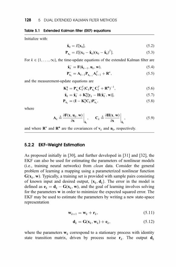
Table 5.1 Extended Kalman filter (EKF) equations

Initialize with:

xx0 ¼ E½x0�; ð5:2Þ

Px0¼ E½ðx0 � xx0Þðx0 � xx0Þ

T�: ð5:3Þ

For k 2 1; . . . ;1gf , the time-update equations of the extended Kalman filter are

xx�k ¼ Fðxxk�1; uk;wÞ; ð5:4Þ

P�xk¼ Ak�1Pxk�1

ATk�1 þ Rv; ð5:5Þ

and the measurement-update equations are

Kxk ¼ P�

xkCT

k ðCkP�xk

CTk þ RnÞ

�1; ð5:6Þ

xxk ¼ xx�k þ Kx

k ½yk � Hðxx�k ;wÞ�; ð5:7Þ

Pxk¼ ðI � Kx

kCkÞP�xk; ð5:8Þ

where

Ak ¼D @Fðx; uk;wÞ

@x

��xxk

; Ck ¼D @Hðx;wÞ

@x

��xxk

; ð5:9Þ

and where Rv and Rn are the covariances of vk and nk, respectively.


corresponds to a nonlinear observation on wk . The EKF can then be

applied directly, with the equations given in Table 5.2. In the linear case,

the relationship between the Kalman filter (KF) and the popular recursive

least-squares (RLS) is given [33] and [34]. In the nonlinear case, the EKF

training corresponds to a modified-Newton optimization method [22].

As an optimization approach, the EKF minimizes the prediction error

cost:

J ðwÞ ¼Pkt¼1

½dt � Gðxt;wÞ�TðReÞ

�1½dt � Gðxt;wÞ�: ð5:21Þ

If the ‘‘noise’’ covariance Re is a constant diagonal matrix, then, in fact, it

cancels out of the algorithm (this can be shown explicitly), and hence can

be set arbitrarily (e.g., Re ¼ 0:5I). Alternatively, Re can be set to specify a

weighted MSE cost. The innovations covariance E½rkrTk � ¼ Rr

k , on the

other hand, affects the convergence rate and tracking performance.

Roughly speaking, the larger the covariance, the more quickly older

data are discarded. There are several options on how to choose Rrk :

Set Rrk to an arbitrary diagonal value, and anneal this towards zeroes

as training continues.

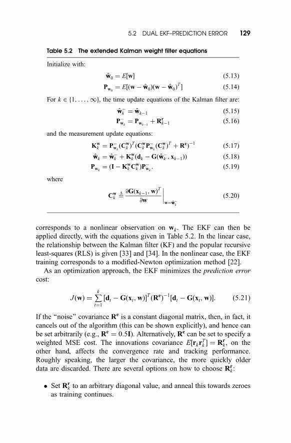
Table 5.2 The extended Kalman weight filter equations

Initialize with:

ww0 ¼ E½w� ð5:13Þ

Pw0¼ E½ðw � ww0Þðw � ww0Þ

T� ð5:14Þ

For k 2 1; . . . ;1f g, the time update equations of the Kalman filter are:

ww�k ¼ wwk�1 ð5:15Þ

P�wk

¼ Pwk�1þ Rr

k�1 ð5:16Þ

and the measurement update equations:

Kwk ¼ P�

wkðCw

k ÞTðCw

k P�wkðCw

k ÞTþ ReÞ

�1ð5:17Þ

wwk ¼ ww�k þ Kw

k ðdk � Gðww�k ; xk�1ÞÞ ð5:18Þ

Pwk¼ ðI � Kw

k Cwk ÞP

�wk: ð5:19Þ

where

Cwk ¼

D @Gðxk�1;wÞT

@w

��w¼ww�

k

ð5:20Þ


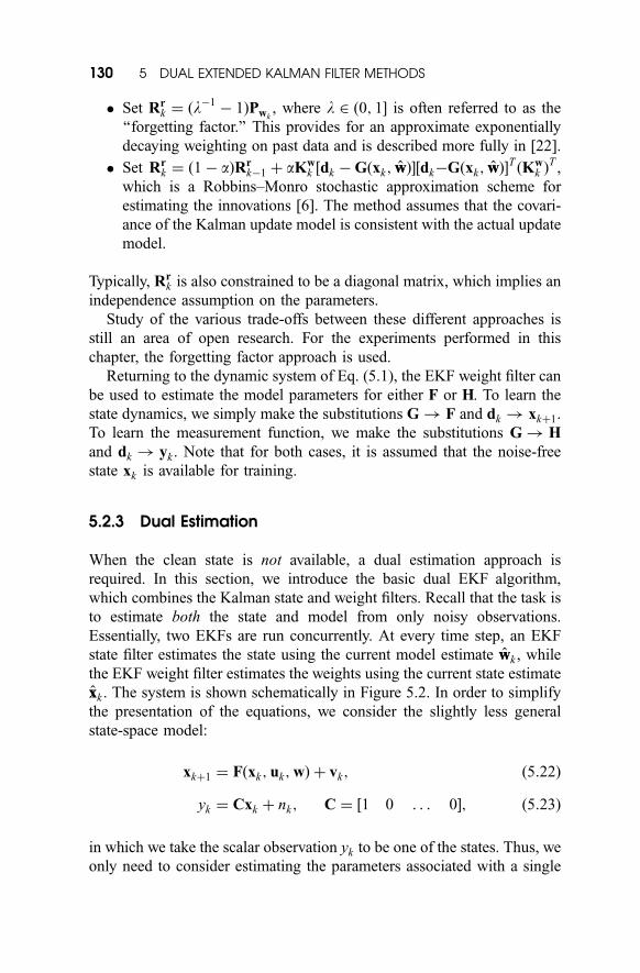
Set Rrk ¼ ðl�1

� 1ÞPwk, where l 2 ð0; 1� is often referred to as the

‘‘forgetting factor.’’ This provides for an approximate exponentially

decaying weighting on past data and is described more fully in [22].

Set Rrk ¼ ð1 � aÞRr

k�1 þ aKwk ½dk � Gðxk; wwÞ�½dk�Gðxk; wwÞ�

TðKw

k ÞT ,

which is a Robbins–Monro stochastic approximation scheme for

estimating the innovations [6]. The method assumes that the covari-

ance of the Kalman update model is consistent with the actual update

model.

Typically, Rrk is also constrained to be a diagonal matrix, which implies an

independence assumption on the parameters.

Study of the various trade-offs between these different approaches is

still an area of open research. For the experiments performed in this

chapter, the forgetting factor approach is used.

Returning to the dynamic system of Eq. (5.1), the EKF weight filter can

be used to estimate the model parameters for either F or H. To learn the

state dynamics, we simply make the substitutions G ! F and dk ! xkþ1.

To learn the measurement function, we make the substitutions G ! H

and dk ! yk . Note that for both cases, it is assumed that the noise-free

state xk is available for training.

5.2.3 Dual Estimation

When the clean state is not available, a dual estimation approach is

required. In this section, we introduce the basic dual EKF algorithm,

which combines the Kalman state and weight filters. Recall that the task is

to estimate both the state and model from only noisy observations.

Essentially, two EKFs are run concurrently. At every time step, an EKF

state filter estimates the state using the current model estimate wwk , while

the EKF weight filter estimates the weights using the current state estimate

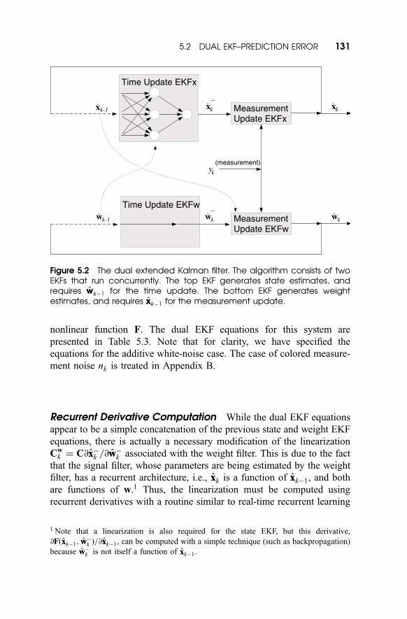
xxk . The system is shown schematically in Figure 5.2. In order to simplify

the presentation of the equations, we consider the slightly less general

state-space model:

xkþ1 ¼ Fðxk;uk;wÞ þ vk; ð5:22Þ

yk ¼ Cxk þ nk; C ¼ ½1 0 . . . 0�; ð5:23Þ

in which we take the scalar observation yk to be one of the states. Thus, we

only need to consider estimating the parameters associated with a single


nonlinear function F. The dual EKF equations for this system are

presented in Table 5.3. Note that for clarity, we have specified the

equations for the additive white-noise case. The case of colored measure-

ment noise nk is treated in Appendix B.

Recurrent Derivative Computation While the dual EKF equations

appear to be a simple concatenation of the previous state and weight EKF

equations, there is actually a necessary modification of the linearization

Cwk ¼ C@xx�

k =@ww�k associated with the weight filter. This is due to the fact

that the signal filter, whose parameters are being estimated by the weight

filter, has a recurrent architecture, i.e., xxk is a function of xxk�1, and both

are functions of w.1 Thus, the linearization must be computed using

recurrent derivatives with a routine similar to real-time recurrent learning

xk-1 MeasurementUpdate EKFx

MeasurementUpdate EKFw

x xk

yk

k

www kk-1

Time Update EKFx

Time Update EKFw

(measurement)

k

−

−

∧ ∧ ∧

∧∧∧

Figure 5.2 The dual extended Kalman filter. The algorithm consists of twoEKFs that run concurrently. The top EKF generates state estimates, andrequires wwk�1 for the time update. The bottom EKF generates weightestimates, and requires xxk�1 for the measurement update.

1 Note that a linearization is also required for the state EKF, but this derivative,

@Fðxxk�1; ww�k Þ=@xxk�1, can be computed with a simple technique (such as backpropagation)

because ww�k is not itself a function of xxk�1.


(RTRL) [35]. Taking the derivative of the signal filter equations results in

the following system of recursive equations:

@xx�kþ1

@ww¼

@Fðxx; wwÞ

@xxk

@xxk

@wwþ@Fðxx; wwÞ

@wwk

; ð5:35Þ

@xxk

@ww¼ ðI � Kx

kCÞ@xx�

k

@wwþ@Kx

k

@wwðyk � Cxx�k Þ; ð5:36Þ

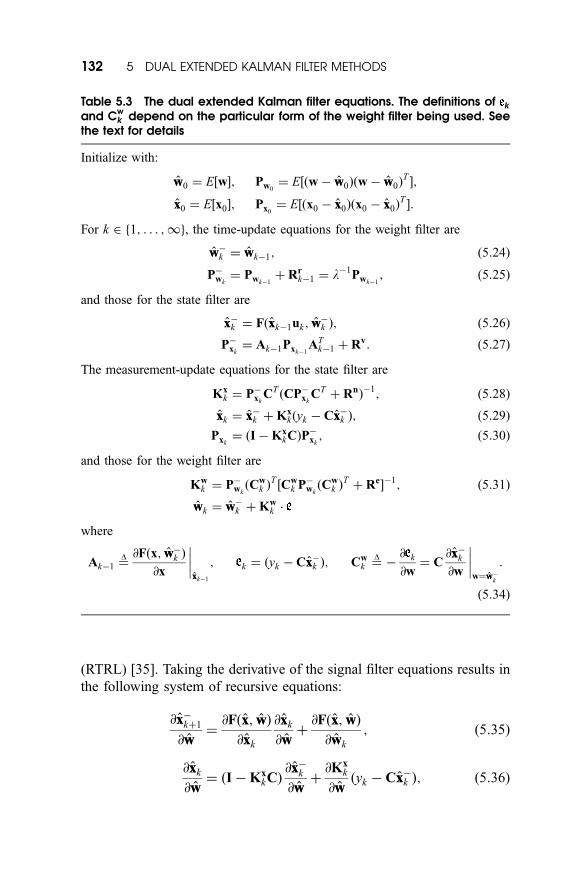
Table 5.3 The dual extended Kalman filter equations. The definitions of k

and Cwk depend on the particular form of the weight filter being used. See

the text for details

Initialize with:

ww0 ¼ E½w�; Pw0¼ E½ðw � ww0Þðw � ww0Þ

T�;

xx0 ¼ E½x0�; Px0¼ E½ðx0 � xx0Þðx0 � xx0Þ

T�:

For k 2 1; . . . ;1gf , the time-update equations for the weight filter are

ww�k ¼ wwk�1; ð5:24Þ

P�wk

¼ Pwk�1þ Rr

k�1 ¼ l�1Pwk�1; ð5:25Þ

and those for the state filter are

xx�k ¼ Fðxxk�1uk ; ww�

k Þ; ð5:26Þ

P�xk¼ Ak�1Pxk�1

ATk�1 þ Rv: ð5:27Þ

The measurement-update equations for the state filter are

Kxk ¼ P�

xkCT

ðCP�xk

CTþ RnÞ

�1; ð5:28Þ

xxk ¼ xx�k þ Kx

kðyk � Cxx�k Þ; ð5:29Þ

Pxk¼ ðI � Kx

kCÞP�xk; ð5:30Þ

and those for the weight filter are

Kwk ¼ P�

wkðCw

k ÞT½Cw

k P�wkðCw

k ÞTþ Re�

�1; ð5:31Þ

wwk ¼ ww�k þ Kw

k �

where

Ak�1 ¼D @Fðx; ww�

k Þ

@x

��xxk�1

; k ¼ ðyk � Cxx�k Þ; Cw

k ¼D�@ k

@w¼ C

@xx�k

@w

��w¼ww�

k

:

ð5:34Þ


where @Fðxx; wwÞ=@xxk and @Fðxx; wwÞ=@wwk are evaluated at wwk and contain

static linearizations of the nonlinear function.

The last term in Eq. (5.36) may be dropped if we assume that the

Kalman gain Kxk is independent of w. Although this greatly simplifies the

algorithm, the exact computation of @Kxk=@ww may be computed, as shown

in Appendix A. Whether the computational expense in calculating the

recursive derivatives (especially that of calculating @Kxk=@ww) is worth the

improvement in performance is clearly a design issue. Experimentally,

the recursive derivatives appear to be more critical when the signal is

highly nonlinear, or is corrupted by a high level of noise.

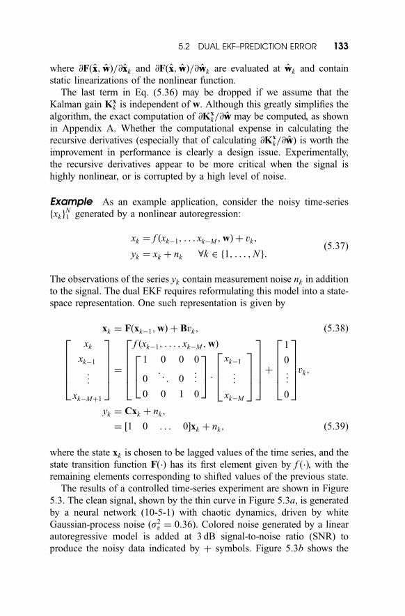
Example As an example application, consider the noisy time-series

fxkgN1 generated by a nonlinear autoregression:

xk ¼ f ðxk�1; . . . xk�M ;wÞ þ vk;

yk ¼ xk þ nk 8k 2 f1; . . . ;Ng:ð5:37Þ

The observations of the series yk contain measurement noise nk in addition

to the signal. The dual EKF requires reformulating this model into a state-

space representation. One such representation is given by

xk ¼ Fðxk�1;wÞ þ Bvk; ð5:38Þ

xk

xk�1

..

.

xk�Mþ1

266664

377775 ¼

f ðxk�1; . . . ; xk�M ;wÞ

1 0 0 0

0 . ..

0 ...

0 0 1 0

264

375 �

xk�1

..

.

xk�M

2664

3775

266664

377775þ

1

0

..

.

0

266664

377775vk;

yk ¼ Cxk þ nk;

¼ ½1 0 . . . 0�xk þ nk; ð5:39Þ

where the state xk is chosen to be lagged values of the time series, and the

state transition function Fð�Þ has its first element given by f ð�Þ, with the

remaining elements corresponding to shifted values of the previous state.

The results of a controlled time-series experiment are shown in Figure

5.3. The clean signal, shown by the thin curve in Figure 5.3a, is generated

by a neural network (10-5-1) with chaotic dynamics, driven by white

Gaussian-process noise (s2v ¼ 0:36). Colored noise generated by a linear

autoregressive model is added at 3 dB signal-to-noise ratio (SNR) to

produce the noisy data indicated by þ symbols. Figure 5.3b shows the


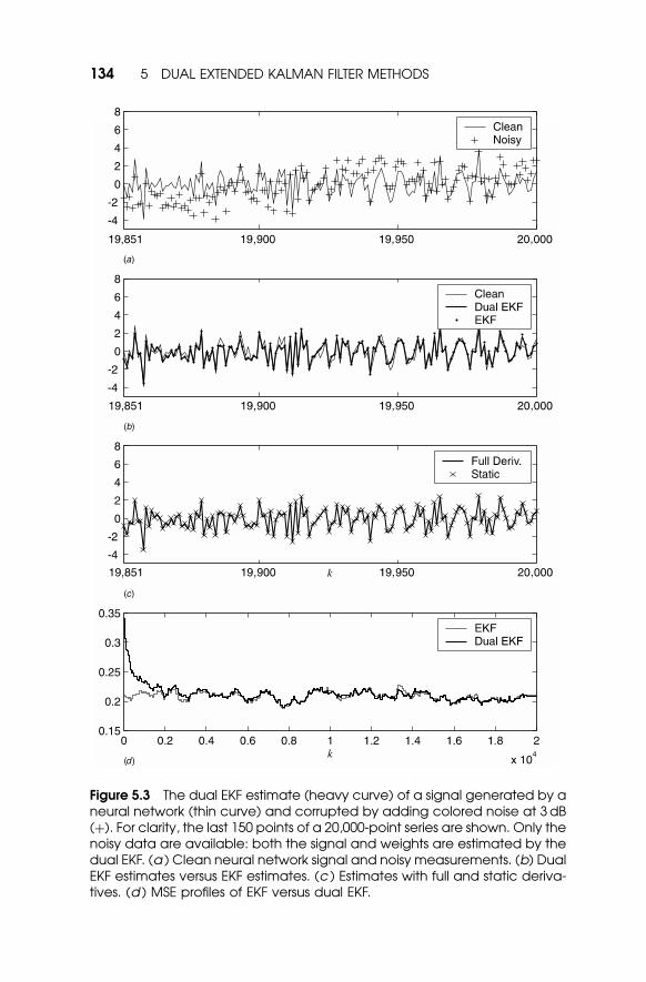
Figure 5.3 The dual EKF estimate (heavy curve) of a signal generated by aneural network (thin curve) and corrupted by adding colored noise at 3 dB(þ). For clarity, the last 150 points of a 20,000-point series are shown. Only thenoisy data are available: both the signal and weights are estimated by thedual EKF. (a ) Clean neural network signal and noisy measurements. (b) DualEKF estimates versus EKF estimates. (c ) Estimates with full and static deriva-tives. (d ) MSE profiles of EKF versus dual EKF.


time series estimated by the dual EKF. The algorithm estimates both the

clean time series and the neural network weights. The algorithm is run

sequentially over 20,000 points of data; for clarity, only the last 150 points

are shown. For comparison, the estimates using an EKF with the known

neural network model are also shown. The MSE for the dual EKF,

computed over the final 1000 points of the series, is 0.2171, whereas

the EKF produces an MSE of 0.2153, indicating that the dual algorithm

has successfully learned both the model and the states estimates.2

Figure 5.3c shows the estimate when the static approximation to

recursive derivatives is used. In this example, this static derivative actually

provides a slight advantage, with an MSE of 0.2122. The difference,

however, is not statistically significant. Finally, Figure 5.3d assesses the

convergence behavior of the algorithm. The mean-squared error (MSE) is

computed over 500 point segments of the time series at 50 point intervals

to produce the MSE profile (dashed line). For comparison, the solid line is

the MSE profile of the EKF signal estimation algorithm, which uses the

true neural network model. The dual EKF appears to converge to the

optimal solution after only about 2000 points.

5.3 A PROBABILISTIC PERSPECTIVE

In this section, we present a unified framework for dual estimation. We

start by developing a probabilistic perspective, which leads to a number of

possible cost functions that can be used in the estimation process. Various

approaches in the literature, which may differ in their actual optimization

procedure, can then be related based on the underlying cost function. We

then show how a Kalman-based optimization procedure can be used to

provide a common algorithmic framework for minimizing each of the cost

functions.

MAP Estimation Dual estimation can be cast as a maximum a poster-

iori (MAP) solution. The statistical information contained in the sequence

of data fykgN1 about the signal and parameters is embodied by the joint

conditional probability density of the sequence of states fxkgN1 and weights

2 A surprising result is that the dual EKF sometimes actually outperforms the EKF, even

though the EKF appears to have an unfair advantage of knowing the true model. Our

explanation is that the EKF, even with the known model, is still an approximate estimation

algorithm. While the dual EKF also learns an approximate model, this model can actually

be better matched to the state estimation approximation.

5.3 A PROBABILISTIC PERSPECTIVE 135

w, given the noisy data fykgN1 . For notational convenience, define the

column vectors xN1 and yN

1 , with elements from fxkgN1 and fykg

N1 ,

respectively. The joint conditional density function is written as

rxN1

wjyN1ðX ¼ xN

1 ; W ¼ wjY ¼ yN1 Þ; ð5:40Þ

where X, Y, and W are the vectors of random variables associated with

xN1 , yN

1 , and w, respectively. This joint density is abbreviated as rxN1

wjyN1.

The MAP estimation approach consists of determining instances of the

states and weights that maximize this conditional density. For Gaussian

distributions, the MAP estimate also corresponds to the minimum mean-

squared error (MMSE) estimator. More generally, as long as the density is

unimodal and symmetric around the mean, the MAP estimate provides the

Bayes estimate for a broad class of loss functions [36].

Taking MAP as the starting point allows dual estimation approaches to

be divided into two basic classes. The first, referred to here as joint

estimation methods, attempt to maximize rxN1

wjyN1

directly. We can write

this optimization problem explicitly as

ðxxN1 ; wwÞ ¼ arg max

xN1;wrxN

1wjyN

1: ð5:41Þ

The second class of methods, which will be referred to as marginal

estimation methods, operate by expanding the joint density as

rxN1

wjyN1¼ rxN

1jwyN

1rwjyN

1ð5:42Þ

and maximizing the two terms separately, that is,

xxN1 ¼ arg max

xN1

rxN1jwyN

1; ww ¼ arg max

wrwjyN

1: ð5:43Þ

The cost functions associated with joint and marginal approaches will be

discussed in the following sections.


5.3.1 Joint Estimation Methods

Using Bayes’ rule, the joint conditional density can be expressed as

rxN1

wjyN1¼

ryN1jxN

1wrxN

1w

ryN1

¼ryN

1jxN

1wrxN

1jwrw

ryN1

: ð5:44Þ

Although fykgN1 is statistically dependent on fxkg

N1 and w, the prior ryN

1is

nonetheless functionally independent of fxkgN1 and w. Therefore, rxN

1wjyN

1

can be maximized by maximizing the terms in the numerator alone.

Furthermore, if no prior information is available on the weights, rw can be

dropped, leaving the maximization of

ryN1

xN1jw ¼ ryN

1jxN

1wrxN

1jw ð5:45Þ

with respect to fxkgN1 and w.

To derive the corresponding cost function, we assume vk and nk are

both zero-mean white Gaussian noise processes. It can then be shown (see

[22]), that

ryN1

xN1jw ¼

1ffiffiffiffiffiffiffiffiffiffiffiffiffiffiffiffiffiffiffiffiffiffið2pÞN ðs2

nÞN

q exp �PNk¼1

ðyk � CxkÞ2

2s2n

" #

�1ffiffiffiffiffiffiffiffiffiffiffiffiffiffiffiffiffiffiffiffiffiffiffi

ð2pÞN jRvjNq exp �

PNk¼1

1

2ðxk � x�

k ÞTðRvÞ

�1ðxk � x�k Þ

� �;

ð5:46Þ

where

x�k ¼

DE½xk jfxtg

k�11 ;w� ¼ Fðxk�1;wÞ: ð5:47Þ


Here we have used the structure given in Eq. (5.37) to compute the

prediction x�k using the model Fð�;wÞ. Taking the logarithm, the corre-

sponding cost function is given by

J ¼PNk¼1

logð2ps2nÞ þ

ðyk � CxkÞ2

s2n

"ð5:48Þ

þ logð2pjRvjÞ þ ðxk � x�k ÞTðRvÞ

�1ðxk � x�

k Þ

�: ð5:49Þ

This cost function can be minimized with respect to any of the unknown

quantities (including the variances, which we will consider in Section 5.4).

For the time being, consider only the optimization of fxkgN1 and w.

Because the log terms in the above cost are independent of the signal

and weights, they can be dropped, providing a more specialized cost

function:

J jðxN1 ;wÞ ¼

PNk¼1

ðyk � CxkÞ2

s2n

þ ðxk � x�k ÞTðRvÞ

�1ðxk � x�

k Þ

" #: ð5:50Þ

The first term is a soft constraint keeping fxkgN1 close to the observations

fykgN1 . The smaller the measurement noise variance s2

n, the stronger this

constraint will be. The second term keeps the state estimates and model

estimates mutually consistent with the model structure. This constraint

will be strong when the state is highly deterministic (i.e., Rv is small).

J jðxN1 ;wÞ should be minimized with respect to both fxkg

N1 and w to find

the estimates that maximize the joint density ryN1

xN1jw. This is a difficult

optimization problem because of the high degree of coupling between the

unknown quantities fxkgN1 and w. In general, we can classify approaches as

being either direct or decoupled. In direct approaches, both the signal and

the state are determined jointly as a multivariate optimization problem.

Decoupled approaches optimize one variable at a time while the other

variable is fixed, and then alternating. Direct algorithms include the joint

EKF algorithm (see Section 5.1), which attempts to minimize the cost

sequentially by combining the signal and weights into a single (joint) state

vector. The decoupled approaches are elaborated below.

Decoupled Estimation To minimize J jðxN1 ;wÞ with respect to the

signal, the cost function is evaluated using the current estimate ww of the


weights to generate the predictions. The simplest approach is to substitute

the predictions xx�k ¼D Fðxk�1; wwÞ directly into Eq. (5.50), obtaining

J jðxN1 ; wwÞ ¼

PNk¼1

ðyk � CxkÞ2

s2n

þ ðxk � xx�k ÞTðRvÞ

�1ðxk � xx�

k Þ

" #: ð5:51Þ

This cost function is then minimized with respect to fxkgN1 . To minimize

the joint cost function with respect to the weights, J jðxN1 ;wÞ is evaluated

using the current signal estimate fxxkgN1 and the associated (redefined)

predictions xx�k ¼D Fðxxk�1;wÞ. Again, this results in a straightforward

substitution in Eq. (5.50):

J jðxxN1 ;wÞ ¼

PNk¼1

ðyk � CxxkÞ2

s2n

þ ðxxk � xx�k ÞTðRvÞ

�1ðxxk � xx�

k Þ

" #: ð5:52Þ

An alternative simplified cost function can be used if it is assumed that

only xx�k is a function of the weights:

Jji ðxx

N1 ;wÞ ¼

PNk¼1

ðxxk � xx�k ÞTðRvÞ

�1ðxxk � xx�

k Þ: ð5:53Þ

This is essentially a type of prediction error cost, where the model is

trained to predict the estimated state. Effectively, the method maximizes

rxN1jw, evaluated at xN

1 ¼ xxN1 . A potential problem with this approach is

that it is not directly constrained by the actual data fykgN1 . An inaccurate

(yet self-consistent) pair of estimates ðxxN1 ; wwÞ could conceivably be

obtained as a solution. Nonetheless, this is essentially the approach used

in [14] for robust prediction of time series containing outliers.

In the decoupled approach to joint estimation, by separately minimizing

each cost with respect to its argument, the values are found that maximize

(at least locally) the joint conditional density function. Algorithms that fall

into this class include a sequential two-observation form of the dual EKF

algorithm [21], and the errors-in-variables (EIV) method applied to batch-

style minimization [18, 19]. An alternative approach, referred to as error

coupling, makes the extra step of taking the errors in the estimates into

account. However, this error-coupled approach (investigated in [22]) does

not appear to perform reliably, and is not described further in this chapter.


5.3.2 Marginal Estimation Methods

Recall that in marginal estimation, the joint density function is expanded

as

rxN1

wjyN1¼ rxN

1jwyN

1rwjyN

1; ð5:54Þ

and xxN1 is found by maximizing the first factor on the right-hand side,

while ww is found by maximizing the second factor. Note that only the first

factor (rxN1jwyN

1) is dependent on the state. Hence, maximizing this factor

for the state will yield the same solution as when maximizing the joint

density (assuming the optimal weights have been found). However,

because both factors also depend on w, maximizing the second (rwjyN1)

alone with respect to w is not the same as maximizing the joint density

rxN1

wjyN1

with respect to w. Nonetheless, the resulting estimates ww are

consistent and unbiased, if conditions of sufficient excitation are met [37].

The marginal estimation approach is exemplified by the maximum-

likelihood approaches [8, 9] and EM approaches [11, 12]. Motivation for

these methods usually comes from considering only the marginal density

rwjyN1

to be the relevant quantity to maximize, rather than the joint density

rxN1

wjyN1. However, in order to maximize the marginal density, it is

necessary to generate signal estimates that are invariably produced by

maximizing the first term rxN1jwyN

1.

Maximum-Likelihood Cost To derive a cost function for weight

estimation, we further expand the marginal density as

rwjyN1¼

ryN1jwrw

ryN1

: ð5:55Þ

If there is no prior information on w, maximizing this posterior density is

equivalent to maximizing the likelihood function ryN1jw. Assuming Gaus-

sian statistics, the chain rule for conditional probabilities can be used to

express this likelihood function as:

ryN1jw ¼

QNk¼1

1ffiffiffiffiffiffiffiffiffiffiffi2ps2

ek

q exp �ðyk � ykjk�1Þ

2

2s2ek

" #; ð5:56Þ


where

ykjk�1 ¼D

E½yk j yt

� �k�1

1;w� ð5:57Þ

is the conditional mean (and optimal prediction), and s2ek

is the predic-

tion error variance. Taking the logarithm yields the following maximum-

likelihood cost function:

J mlðwÞ ¼PNk¼1

logð2ps2ekÞ þ

ðyk � ykjk�1Þ2

s2ek

" #: ð5:58Þ

Note that the log-likelihood function takes the same form whether the

measurement noise is colored or white. In evaluating this cost function,

the term ykjk�1 ¼ Cxx�k must be computed. Thus, the signal estimate must

be determined as a step to weight estimation. For linear models, this can

be done exactly using an ordinary Kalman filter. For nonlinear models,

however, the expectation is approximated by an extended Kalman filter,

which equivalently attempts to minimize the joint cost J jðxk1; wwÞ defined in

Section 5.3.1 by Eq. (5.51).

An iterative maximum-likelihood approach for linear models is

described in [7] and [8]; this chapter presents a sequential maximum-

likelihood approach for nonlinear models, developed in [21].

Prediction Error Cost Often the variance s2ek

in the maximum-like-

lihood cost is assumed (incorrectly) to be independent of the weights w

and the time index k. Under this assumption, the log likelihood can be

maximized by minimizing the squared prediction error cost function:

J peðwÞ ¼PNk¼1

ðyk � ykjk�1Þ2: ð5:59Þ

The basic dual EKF algorithm described in the previous section minimizes

this simplified cost function with respect to the weights w, and is an

example of a recursive prediction error algorithm [6, 19]. While ques-

tionable from a theoretical perspective, these algorithms have been shown

in the literature to be quite useful. In addition, they benefit from reduced

computational cost, because the derivative of the variance s2ek

with respect

to w is not computed.


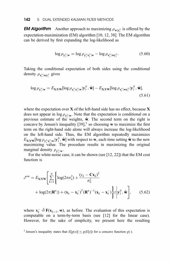
EM Algorithm Another approach to maximizing rwjyN1

is offered by the

expectation-maximization (EM) algorithm [10, 12, 38]. The EM algorithm

can be derived by first expanding the log-likelihood as

log ryN1jw ¼ log ryN

1xN

1jw � log rxN

1jwyN

1: ð5:60Þ

Taking the conditional expectation of both sides using the conditional

density rxN1jwyN

1gives

logryN1jw ¼ EXjYW½logryN

1xN

1jwjy

N1 ; ww� � EXjYW½logrxN

1jwyN

1jyN

1 ; ww�;

ð5:61Þ

where the expectation over X of the left-hand side has no effect, because X

does not appear in logryN1jw. Note that the expectation is conditional on a

previous estimate of the weights, ww. The second term on the right is

concave by Jensen’s inequality [39],3 so choosing w to maximize the first

term on the right-hand side alone will always increase the log-likelihood

on the left-hand side. Thus, the EM algorithm repeatedly maximizes

EXjYW½log ryN1

xN1jwjy

N1 ; ww� with respect to w, each time setting ww to the new

maximizing value. The procedure results in maximizing the original

marginal density ryN1jw .

For the white-noise case, it can be shown (see [12, 22]) that the EM cost

function is

J em ¼ EXjYW

PNk¼1

logð2ps2nÞ þ

ðyk � CxkÞ2

s2n

("

þ logð2pjRvjÞ þ ðxk � x�k ÞTðRvÞ

�1ðxk � x�

k Þ

)z

��yN1 ; ww

#; ð5:62Þ

where x�k ¼

D Fðxk�1;wÞ, as before. The evaluation of this expectation is

computable on a term-by-term basis (see [12] for the linear case).

However, for the sake of simplicity, we present here the resulting

3 Jensen’s inequality states that E½gðxÞ� � gðE½x�Þ for a concave function gð�Þ.


expression for the special case of time-series estimation, represented in

Eq. (5.37). As shown in [22], the expectation evaluates to

J em ¼ N logð4p2s2vs

2nÞ þ

PNk¼1

ðyk � xxkjN Þ2þ pkjN

s2n

"

þðxxkjN � xx�kjN Þ

2þ pkjN � 2p

y

kjN þ p�kjN

s2v

#; ð5:63Þ

where xxkjN and pkjN are defined as the conditional mean and variance of xk

given ww and all the data, fykgN1 . The terms xx�kjN and p�kjN are the conditional

mean and variance of x�k ¼ f ðxk�1;wÞ, given all the data. The additional

term py

kjN represents the cross-variance of xk and x�k , conditioned on all the

data. Again we see that determining state estimates is a necessary step to

determining the weights. In this case, the estimates xxkjN are found by

minimizing the joint cost J jðxN1 ; wwÞ, which can be approximated using an

extended Kalman smoother. A sequential version of EM can be imple-

mented by replacing xxkjN with the usual causal estimates xxk , found using

the EKF.

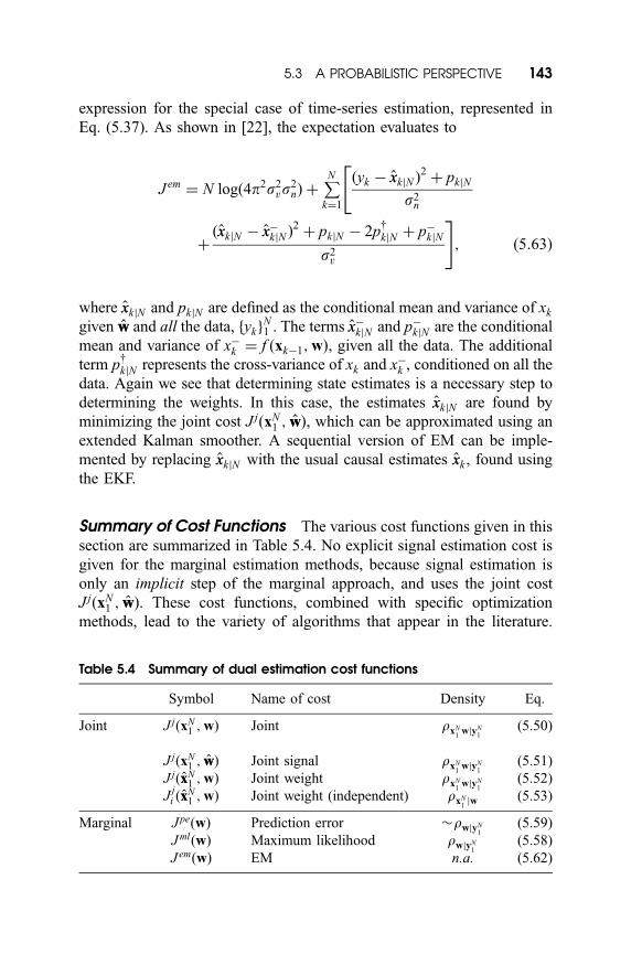
Summary of Cost Functions The various cost functions given in this

section are summarized in Table 5.4. No explicit signal estimation cost is

given for the marginal estimation methods, because signal estimation is

only an implicit step of the marginal approach, and uses the joint cost

J jðxN1 ; wwÞ. These cost functions, combined with specific optimization

methods, lead to the variety of algorithms that appear in the literature.

Table 5.4 Summary of dual estimation cost functions

Symbol Name of cost Density Eq.

Joint J jðxN1 ;wÞ Joint rxN

1wjyN

1(5.50)

J jðxN1 ; wwÞ Joint signal rxN

1wjyN

1(5.51)

J jðxxN1 ;wÞ Joint weight rxN

1wjyN

1(5.52)

Jji ðxx

N1 ;wÞ Joint weight (independent) rxN

1jw (5.53)

Marginal J peðwÞ Prediction error �rwjyN1

(5.59)

J mlðwÞ Maximum likelihood rwjyN1

(5.58)

J emðwÞ EM n.a. (5.62)


In the next section, we shall show how each of these cost functions can be

minimized using a general dual EKF-based approach.

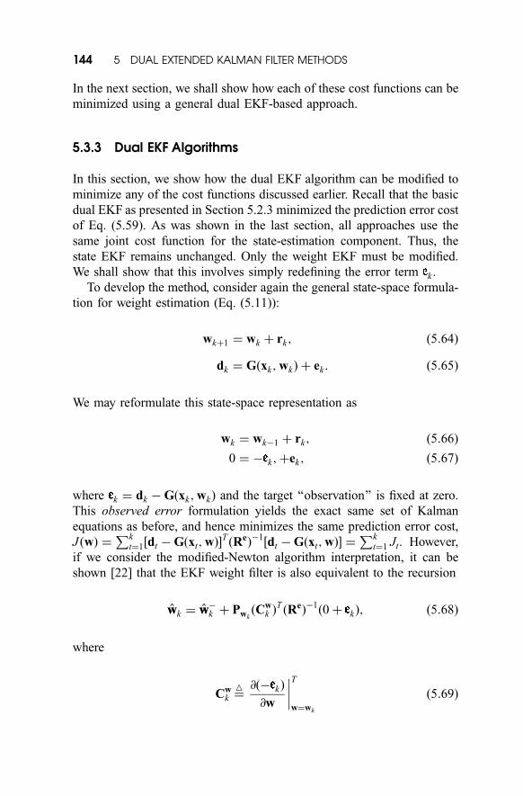
5.3.3 Dual EKF Algorithms

In this section, we show how the dual EKF algorithm can be modified to

minimize any of the cost functions discussed earlier. Recall that the basic

dual EKF as presented in Section 5.2.3 minimized the prediction error cost

of Eq. (5.59). As was shown in the last section, all approaches use the

same joint cost function for the state-estimation component. Thus, the

state EKF remains unchanged. Only the weight EKF must be modified.

We shall show that this involves simply redefining the error term k .

To develop the method, consider again the general state-space formula-

tion for weight estimation (Eq. (5.11)):

wkþ1 ¼ wk þ rk; ð5:64Þ

dk ¼ Gðxk;wkÞ þ ek : ð5:65Þ

We may reformulate this state-space representation as

wk ¼ wk�1 þ rk; ð5:66Þ

0 ¼ � k;þek; ð5:67Þ

where k ¼ dk � Gðxk;wkÞ and the target ‘‘observation’’ is fixed at zero.

This observed error formulation yields the exact same set of Kalman

equations as before, and hence minimizes the same prediction error cost,

J ðwÞ ¼Pk

t¼1½dt � Gðxt;wÞ�TðReÞ

�1½dt � Gðxt;wÞ� ¼

Pkt¼1 Jt. However,

if we consider the modified-Newton algorithm interpretation, it can be

shown [22] that the EKF weight filter is also equivalent to the recursion

wwk ¼ ww�k þ Pwk

ðCwk Þ

TðReÞ

�1ð0 þ kÞ; ð5:68Þ

where

Cwk ¼

4 @ð� kÞ

@w

��T

w¼wk

ð5:69Þ


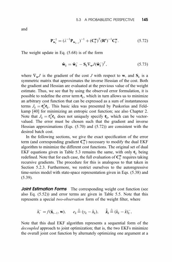
and

P�1wk

¼ ðl�1Pwk�1Þ�1

þ ðCwk Þ

TðReÞ

�1Cwk : ð5:72Þ

The weight update in Eq. (5.68) is of the form

wwk ¼ ww�k � SkHwJ ðww�

k ÞT ; ð5:73Þ

where HwJ is the gradient of the cost J with respect to w, and Sk is a

symmetric matrix that approximates the inverse Hessian of the cost. Both

the gradient and Hessian are evaluated at the previous value of the weight

estimate. Thus, we see that by using the observed error formulation, it is

possible to redefine the error term k , which in turn allows us to minimize

an arbitrary cost function that can be expressed as a sum of instantaneous

terms Jk ¼ Tk k . This basic idea was presented by Puskorius and Feld-

kamp [40] for minimizing an entropic cost function; see also Chapter 2.

Note that Jk ¼ Tk k does not uniquely specify k, which can be vector-

valued. The error must be chosen such that the gradient and inverse

Hessian approximations (Eqs. (5.70) and (5.72)) are consistent with the

desired batch cost.

In the following sections, we give the exact specification of the error

term (and corresponding gradient Cwk ) necessary to modify the dual EKF

algorithm to minimize the different cost functions. The original set of dual

EKF equations given in Table 5.3 remains the same, with only k being

redefined. Note that for each case, the full evaluation of Cwk requires taking

recursive gradients. The procedure for this is analogous to that taken in

Section 5.2.3. Furthermore, we restrict ourselves to the autoregressive

time-series model with state-space representation given in Eqs. (5.38) and

(5.39).

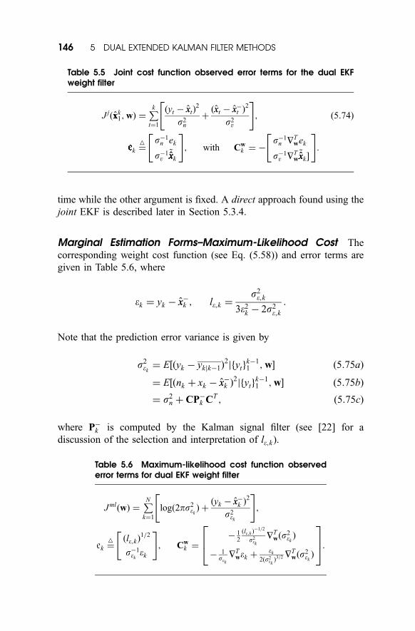
Joint Estimation Forms The corresponding weight cost function (see

also Eq. (5.52)) and error terms are given in Table 5.5. Note that this

represents a special two-observation form of the weight filter, where

xx�t ¼ f ðxxt�1;wÞ; ek ¼4ðyk � xxkÞ;

~xxxxk ¼4ðxxk � xxÞ

�k ;

Note that this dual EKF algorithm represents a sequential form of the

decoupled approach to joint optimization; that is, the two EKFs minimize

the overall joint cost function by alternately optimizing one argument at a


time while the other argument is fixed. A direct approach found using the

joint EKF is described later in Section 5.3.4.

Marginal Estimation Forms–Maximum-Likelihood Cost The

corresponding weight cost function (see Eq. (5.58)) and error terms are

given in Table 5.6, where

ek ¼ yk � xx�k ; le;k ¼s2e;k

3e2k � 2s2

e;k:

Note that the prediction error variance is given by

s2ek¼ E½ðyk � ykjk�1Þ

2jfytg

k�11 ;w� ð5:75aÞ

¼ E½ðnk þ xk � xx�k Þ2jfytg

k�11 ;w� ð5:75bÞ

¼ s2n þ CP�

k CT ; ð5:75cÞ

where P�k is computed by the Kalman signal filter (see [22] for a

discussion of the selection and interpretation of le;k).

Table 5.6 Maximum-likelihood cost function observederror terms for dual EKF weight filter

J mlðwÞ ¼PNk¼1

logð2ps2ekÞ þ

ðyk � xx�k Þ2

s2ek

" #;

ek ¼4 ðle;kÞ

1=2

s�1ekek

" #; Cw

k ¼� 1

2

ðle;k Þ�1=2

s2ek

HTwðs

2ekÞ

� 1sek

HTwek þ

ek

2ðs2ekÞ3=2 HT

wðs2ekÞ

264

375:

Table 5.5 Joint cost function observed error terms for the dual EKFweight filter

J jðxxk1;wÞ ¼

Pkt¼1

ðyt � xxtÞ2

s2n

þðxxt � xx�t Þ

2

s2v

" #; ð5:74Þ

k ¼4 s�1

n ek

s�1v

~xxxxk

" #; with Cw

k ¼ �s�1

n HTwek

s�1v HT

w~xxxxk �

" #:


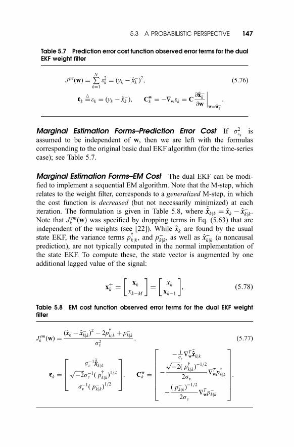
Marginal Estimation Forms–Prediction Error Cost If s2ek

is

assumed to be independent of w, then we are left with the formulas

corresponding to the original basic dual EKF algorithm (for the time-series

case); see Table 5.7.

Marginal Estimation Forms–EM Cost The dual EKF can be modi-

fied to implement a sequential EM algorithm. Note that the M-step, which

relates to the weight filter, corresponds to a generalized M-step, in which

the cost function is decreased (but not necessarily minimized) at each

iteration. The formulation is given in Table 5.8, where ~xxxxkjk ¼ xxk � xx�kjk .

Note that J emk ðwÞ was specified by dropping terms in Eq. (5.63) that are

independent of the weights (see [22]). While xxk are found by the usual

state EKF, the variance terms py

kjk , and p�kjk, as well as xx�kjk (a noncausal

prediction), are not typically computed in the normal implementation of

the state EKF. To compute these, the state vector is augmented by one

additional lagged value of the signal:

xþk ¼xk

xk�M

� �¼

xk

xk�1

� �; ð5:78Þ

Table 5.7 Prediction error cost function observed error terms for the dualEKF weight filter

J peðwÞ ¼PNk¼1

e2k ¼ ðyk � xx�k Þ

2; ð5:76Þ

k ¼4ek ¼ ðyk � xx�k Þ; Cw

k ¼ �Hwek ¼ C@xx�

k

@w

��w¼ww�

k

:

Table 5.8 EM cost function observed error terms for the dual EKF weightfilter

J emk ðwÞ ¼

ðxxk � xx�kjkÞ2� 2p

y

kjk þ p�kjk

s2v

; ð5:77Þ

k ¼

s�1v

~xxxxkjkffiffiffiffiffiffiffi�2

ps�1v ð p

y

kjkÞ1=2

s�1v ð p�

kjkÞ1=2

2664

3775; Cw

k ¼

� 1svHT

w~xxxxkjk

�

ffiffiffiffiffiffiffi�2

pð p

y

kjkÞ�1=2

2svHT

wpy

kjk

�ð p�

kjkÞ�1=2

2svHT

wp�kjk

266666664

377777775:


The state Kalman filter is then modified by adding a final zero element to

the vectors B and C (see Eqs. (5.38) and (5.39)), and the linearized state

transition matrix is redefined as

Ak ¼4 HT

x f

I 0

" #:

Now the estimate xxþk will contain xxk�1jk in its last M elements. As shown

in [22], the variance terms are then approximated by

p�kjk ¼ CAk�1jkðPk�1jkÞATk�1jkCT ; p

y

kjk ¼ CðP]kÞA

Tk�1jkCT ; ð5:79Þ

where the covariance Pk�1jk is provided as the lower right block of the

augmented covariance Pþk , and P

]k is the upper right block of Pþ

k . The

usual error covariance Pk is provided in the upper left block of Pþk .

Furthermore, Ak�1jk is found by linearizing f ð�Þ at xxk�1jk . The noncausal

prediction xx�kjk ¼ E½ f ðxk�1;wÞjfytgk1; ww� � f ðxxk�1jk;wÞ.

Finally, the necessary gradient terms in the dual EKF algorithm can be

evaluated as follows:

HTw~xxxxkjk ¼ �Hwxx�kjk ¼ �Hw f ðxxk�1jk;wÞ; ð5:80Þ

which is evaluated at wwk . The ith element of the gradient vector Hwp�kjk is

constructed from the expression

@p�kjk

@wðiÞ¼ C

@Ak�1jk

@wðiÞðPk�1jkÞA

Tk�1jk þ Ak�1jkðPk�1jkÞ

@ATk�1jk

@wðiÞ

" #CT ; ð5:81Þ

and the elements of the gradient Hwpy

kjk are given by

@py

kjk

@wðiÞ¼ C

@Ak�1jk

@wðiÞðP

]kÞ

T

� �CT : ð5:82Þ

Note that all components in the cost function are recursive functions of ww,

but not of w. Hence, no recurrent derivative computations are required for

the EM algorithm. Furthermore, it can be shown that the actual error

variances p�kjk and p

y

kjk (not their gradients) cancel out in the formula for

Cwk , and thus should be replaced with large constant values to obtain a

good Hessian approximation.


5.3.4 Joint EKF

In the previous section, the dual EKF was modified to minimize the joint

cost function. This implementation represented a decoupled type of

approach, in which separate state-space representations were used to

estimate xk and w. An alternative direct approach is given by the joint

EKF, which generates simultaneous MAP estimates of xk and w. This is

accomplished by defining a new joint state-space representation with

concatenated state:

zk ¼xk

wk

� �: ð5:83Þ

It is clear that maximizing the density rzk jyk1

is equivalent to maximizing

rxk wjyk1. Hence, the MAP-optimal estimate of zk will contain the values of

xk and wk that minimize the batch cost J ðxk1;wÞ. Running the single EKF

with this state vector provides a sequential estimation algorithm. The joint

EKF first appeared in the literature for the estimation of linear systems (in

which there is a bilinear relation between the states and weights) [1, 2].

The general equations for nonlinear systems are given in Table 5.9.

Note that because the gradient of f ðzÞ with respect to w is taken with the

other elements (namely, xxk) fixed, it will not involve recursive derivatives of

xxk with respect to w. This fact is cited in [3] and [6] as a potential source of

convergence problems for the joint EKF. Additional results and citations in

[5] corroborate the difficulties of the approach, although the cause of

divergence is linked there to the linearization of the coupled system, rather

than the lack of recurrent derivatives (note that no divergence problems

were encountered in preparing the experimental results in this chapter).

Although the use of recurrent derivatives is suggested in [3] and [6], there

is no theoretical justification for this. In summary, the joint EKF provides

an alternative to the dual EKF for sequential minimization of the joint cost

function. Note that the joint EKF cannot be readily adapted to minimize

other cost functions discussed in this chapter.

5.4 DUAL EKF VARIANCE ESTIMATION

The implementation of the EKF requires the noise variance, s2v and s2

n as

parameters in the algorithm. Often these can be determined from physical

knowledge of the problem (e.g., sensor accuracy or ambient noise

5.4 DUAL EKF VARIANCE ESTIMATION 149

measurements). However, if the variances are unknown, their values can

be estimated within the dual EKF framework using cost functions similar

to those derived in Section 5.3. A full treatment of the variance estimation

filter is presented in [22]; here we focus on the maximum-likelihood cost

function

J mlðs2Þ ¼PNk¼1

logð2ps2ekÞ þ

ðyk � ykjk�1Þ2

s2ek

" #: ð5:94Þ

Note that this cost function is identical to the weight-estimation cost

function, except that the argument is changed to emphasize the estimation

of the unknown variances.

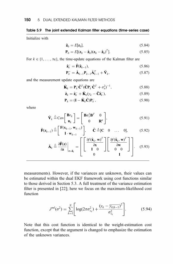
Table 5.9 The joint extended Kalman filter equations (time-series case)

Initialize with

zz0 ¼ E½z0�; ð5:84Þ

P0 ¼ E½ðz0 � zz0Þðz0 � zz0ÞT�: ð5:85Þ

For k 2 1; . . . ;1gf , the time-update equations of the Kalman filter are

zz�k ¼ �FFðzzk�1Þ; ð5:86Þ

P�k ¼ �AAk�1Pk�1

�AATk�1 þ

�VVk; ð5:87Þ

and the measurement update equations are

�KKk ¼ P�k�CCT ð �CCP�

k�CCT þ s2

nÞ�1; ð5:88Þ

zzk ¼ zz�k þ �KKkðyk ��CCzz�k Þ; ð5:89Þ

Pk ¼ ðI � �KKk�CCÞP�

k ; ð5:90Þ

where

�VVk ¼4

CovBvk

uk

� �¼

Bs2vB

T 0

0 Rr

" #; ð5:91Þ

�FFðzk�1Þ ¼4 Fðxk�1;wk�1Þ

I � wk�1

� �; �CC ¼

D½C 0 . . . 0�; ð5:92Þ

�AAk ¼4 @ �FFðzÞ

@z

��z¼zzk

¼

@f ðxxk;wÞT

@xI 0

24

35 @f ðxxk ;wÞ

T

@w0 0

24

35

0 I

2664

3775: ð5:93Þ


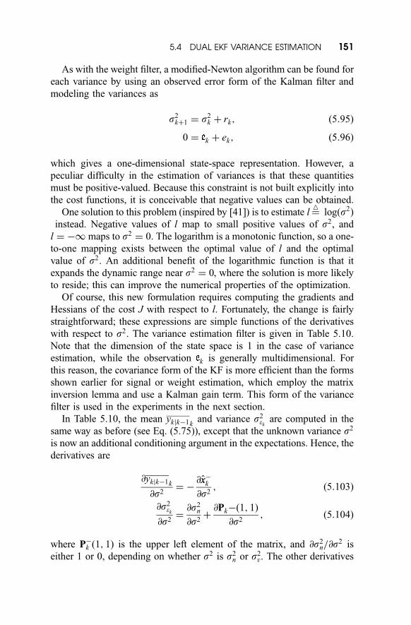
As with the weight filter, a modified-Newton algorithm can be found for

each variance by using an observed error form of the Kalman filter and

modeling the variances as

s2kþ1 ¼ s2

k þ rk; ð5:95Þ

0 ¼ k þ ek; ð5:96Þ

which gives a one-dimensional state-space representation. However, a

peculiar difficulty in the estimation of variances is that these quantities

must be positive-valued. Because this constraint is not built explicitly into

the cost functions, it is conceivable that negative values can be obtained.

One solution to this problem (inspired by [41]) is to estimate l ¼4

logðs2Þ

instead. Negative values of l map to small positive values of s2, and

l ¼ �1 maps to s2 ¼ 0. The logarithm is a monotonic function, so a one-

to-one mapping exists between the optimal value of l and the optimal

value of s2. An additional benefit of the logarithmic function is that it

expands the dynamic range near s2 ¼ 0, where the solution is more likely

to reside; this can improve the numerical properties of the optimization.

Of course, this new formulation requires computing the gradients and

Hessians of the cost J with respect to l. Fortunately, the change is fairly

straightforward; these expressions are simple functions of the derivatives

with respect to s2. The variance estimation filter is given in Table 5.10.

Note that the dimension of the state space is 1 in the case of variance

estimation, while the observation k is generally multidimensional. For

this reason, the covariance form of the KF is more efficient than the forms

shown earlier for signal or weight estimation, which employ the matrix

inversion lemma and use a Kalman gain term. This form of the variance

filter is used in the experiments in the next section.

In Table 5.10, the mean ykjk�1kand variance s2

ekare computed in the

same way as before (see Eq. (5.75)), except that the unknown variance s2

is now an additional conditioning argument in the expectations. Hence, the

derivatives are

@ykjk�1k

@s2¼ �

@xx�k@s2

; ð5:103Þ

@s2ek

@s2¼

@s2n

@s2þ@Pk�ð1; 1Þ

@s2; ð5:104Þ

where P�k ð1; 1Þ is the upper left element of the matrix, and @s2

n=@s2 is

either 1 or 0, depending on whether s2 is s2n or s2

v. The other derivatives

5.4 DUAL EKF VARIANCE ESTIMATION 151

are computed by taking the derivative of the Kalman filter equations with

respect to either variance term (represented by s2). This results in the

following system of recursive equations:

@xx�kþ1

@s2¼

@Fðxx; wwÞ

@xxk

@xxk

@s2; ð5:105Þ

@xxk

@s2¼ ðI � Kx

kCÞ@xx

�

k

@s2þ@Kx

k

@s2ð yk � Cxx�k Þ; ð5:106Þ

where @Fðxx; wwÞ=@xxk is evaluated at wwk , and represents a static linearization

of the neural network. Note that ½@Fðxx; wwÞ=@wwk �½@ww=@s2� does not appear

in Eq. (5.105), under the assumption that @ww=@s2 ¼ 0. The last term in

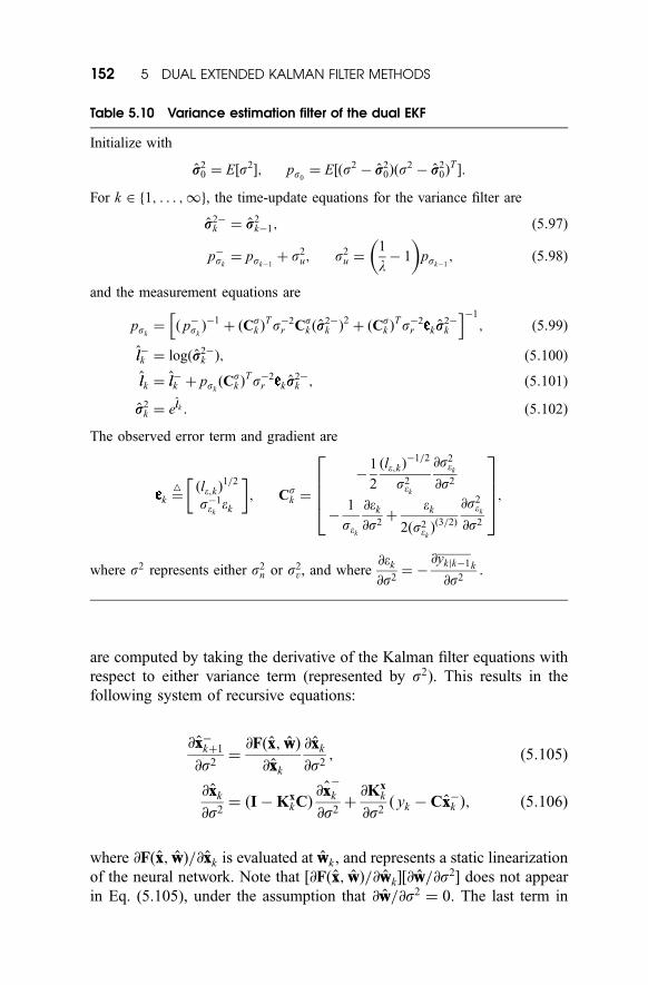
Table 5.10 Variance estimation filter of the dual EKF

Initialize with

ss20 ¼ E½s2�; ps0

¼ E½ðs2 � ss20Þðs

2 � ss20Þ

T�:

For k 2 1; . . . ;1f g, the time-update equations for the variance filter are

ss2�k ¼ ss2

k�1; ð5:97Þ

p�sk

¼ psk�1þ s2

u; s2u ¼

1

l� 1

� �psk�1

; ð5:98Þ

and the measurement equations are

psk¼ ð p�

skÞ�1

þ ðCsk Þ

Ts�2r Cs

k ðss2�k Þ

2þ ðCs

k ÞTs�2

r k ss2�k

h i�1

; ð5:99Þ

ll�k ¼ logðss2�k Þ; ð5:100Þ

llk ¼ ll�k þ pskðCs

k ÞTs�2

r k ss2�k ; ð5:101Þ

ss2k ¼ ellk : ð5:102Þ

The observed error term and gradient are

k ¼4 ðle;kÞ

1=2

s�1ekek

� �; Cs

k ¼

�1

2

ðle;kÞ�1=2

s2ek

@s2ek

@s2

�1

sek

@ek

@s2þ

ek

2ðs2ekÞð3=2Þ

@s2ek

@s2

26664

37775;

where s2 represents either s2n or s2

v, and where@ek

@s2¼ �

@ykjk�1k

@s2:


Eq. (5.106) may be dropped if we assume that the Kalman gain Kx is

independent of s2. However, for accurate computation of the recursive

derivatives, @Kxk=@s

2 must be calculated; this is shown along with the

derivative @P�k ð1; 1Þ=@s2 in Appendix A.

5.5 APPLICATIONS

In this section, we present the results of using the dual EKF methods on a

number of different applications.

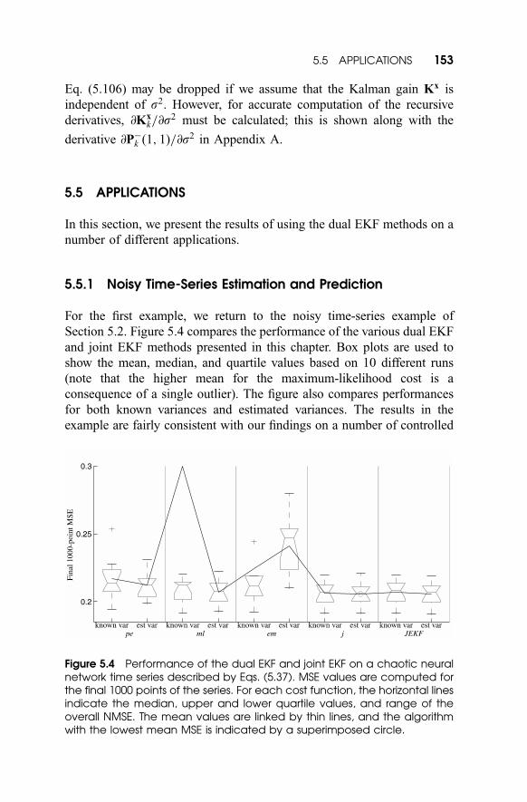
5.5.1 Noisy Time-Series Estimation and Prediction

For the first example, we return to the noisy time-series example of

Section 5.2. Figure 5.4 compares the performance of the various dual EKF

and joint EKF methods presented in this chapter. Box plots are used to

show the mean, median, and quartile values based on 10 different runs

(note that the higher mean for the maximum-likelihood cost is a

consequence of a single outlier). The figure also compares performances

for both known variances and estimated variances. The results in the

example are fairly consistent with our findings on a number of controlled

Figure 5.4 Performance of the dual EKF and joint EKF on a chaotic neuralnetwork time series described by Eqs. (5.37). MSE values are computed forthe final 1000 points of the series. For each cost function, the horizontal linesindicate the median, upper and lower quartile values, and range of theoverall NMSE. The mean values are linked by thin lines, and the algorithmwith the lowest mean MSE is indicated by a superimposed circle.

5.5 APPLICATIONS 153

experiments using different time series and parameter settings [22]. For

both white and colored noises, the maximum-likelihood weight-estimation

cost J mlðwÞ generally produces the best results, but often exhibits

instability. This fact is analyzed in [22], and reduces the desirability of

using this cost function. The joint cost function J jðwÞ has better stability

properties and produces excellent results for colored measurement noise.

For white noise, the prediction error cost performs nearly as well as

J mlðwÞ, but without stability problems. Hence, the dual EKF cost func-

tions J peðwÞ and J jðwÞ are generally the best choices for white and colored

measurement noise, respectively. The joint EKF and dual EKF perform

similarly in many cases, although the joint EKF is considerably less robust

to inaccuracies in the assumed model structure and noise variances.

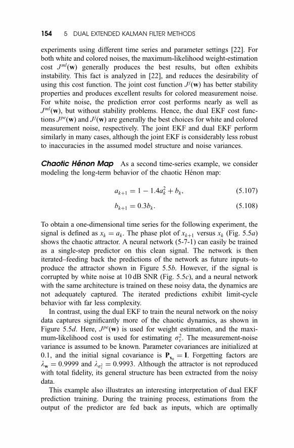
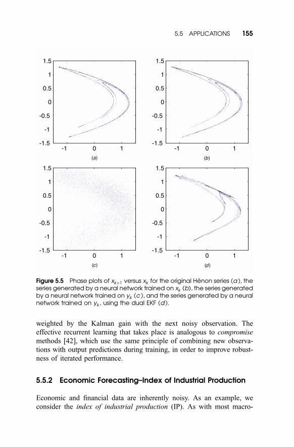
Chaotic Henon Map As a second time-series example, we consider

modeling the long-term behavior of the chaotic Henon map:

akþ1 ¼ 1 � 1:4a2k þ bk; ð5:107Þ

bkþ1 ¼ 0:3bk : ð5:108Þ

To obtain a one-dimensional time series for the following experiment, the

signal is defined as xk ¼ ak . The phase plot of xkþ1 versus xk (Fig. 5.5a)

shows the chaotic attractor. A neural network (5-7-1) can easily be trained

as a single-step predictor on this clean signal. The network is then

iterated–feeding back the predictions of the network as future inputs–to

produce the attractor shown in Figure 5.5b. However, if the signal is

corrupted by white noise at 10 dB SNR (Fig. 5.5c), and a neural network

with the same architecture is trained on these noisy data, the dynamics are

not adequately captured. The iterated predictions exhibit limit-cycle

behavior with far less complexity.

In contrast, using the dual EKF to train the neural network on the noisy

data captures significantly more of the chaotic dynamics, as shown in

Figure 5.5d. Here, J peðwÞ is used for weight estimation, and the maxi-

mum-likelihood cost is used for estimating s2v . The measurement-noise

variance is assumed to be known. Parameter covariances are initialized at

0.1, and the initial signal covariance is Px0¼ I. Forgetting factors are

lw ¼ 0:9999 and ls2v¼ 0:9993. Although the attractor is not reproduced

with total fidelity, its general structure has been extracted from the noisy

data.

This example also illustrates an interesting interpretation of dual EKF

prediction training. During the training process, estimations from the

output of the predictor are fed back as inputs, which are optimally


weighted by the Kalman gain with the next noisy observation. The

effective recurrent learning that takes place is analogous to compromise

methods [42], which use the same principle of combining new observa-

tions with output predictions during training, in order to improve robust-

ness of iterated performance.

5.5.2 Economic Forecasting–Index of Industrial Production

Economic and financial data are inherently noisy. As an example, we

consider the index of industrial production (IP). As with most macro-

-1 0 1-1.5

-1

-0.5

0

0.5

1

1.5

-1 0 1-1.5

-1

-0.5

0

0.5

1

1.5

-1 0 1-1.5

-1

-0.5

0

0.5

1

1.5

-1 0 1-1.5

-1

-0.5

0

0.5

1

1.5

(a)

(c) (d )

(b)

Figure 5.5 Phase plots of xkþ1 versus xk for the original Henon series (a ), theseries generated by a neural network trained on xk (b), the series generatedby a neural network trained on yk (c ), and the series generated by a neuralnetwork trained on yk , using the dual EKF (d ).


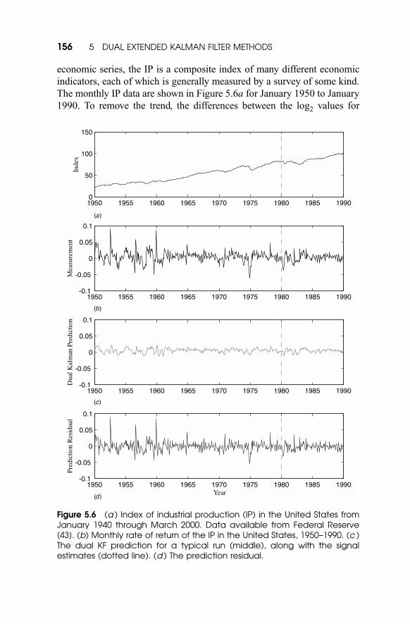
economic series, the IP is a composite index of many different economic

indicators, each of which is generally measured by a survey of some kind.

The monthly IP data are shown in Figure 5.6a for January 1950 to January

1990. To remove the trend, the differences between the log2 values for

Figure 5.6 (a ) Index of industrial production (IP) in the United States fromJanuary 1940 through March 2000. Data available from Federal Reserve[43]. (b) Monthly rate of return of the IP in the United States, 1950–1990. (c )The dual KF prediction for a typical run (middle), along with the signalestimates (dotted line). (d ) The prediction residual.


adjacent months are computed; this is called the IP monthly rate of return,

and is shown in Figure 5.6b.

An important baseline approach is to predict the IP from its past values,

using a standard linear autoregressive model. Results with an AR-14

model are reported by Moody et al. [44]. For comparison, both a linear

AR-14 model and neural network (14 input, 4 hidden unit) model are

tested using the dual EKF methods. Consistent with experiments reported

in [44], data from January 1950 to December 1979 are used for a training

set, and the remainder of the data is reserved for testing. The dual KF (or

dual EKF) is iterated over the training set for several epochs, and the

resultant model–consisting of ww; ss2v , and ss2

n–is used with a standard KF

(or EKF) to produce causal predictions on the test set.

All experiments are repeated 10 times with different initial weights ww0

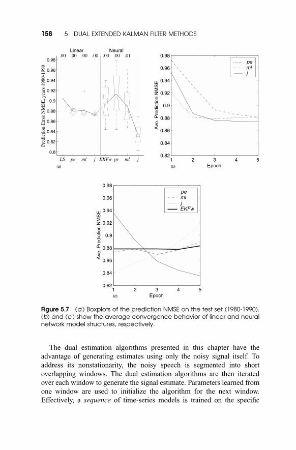
to produce the boxplots in Figure 5.7a. The advantage of dual estimation

on linear models in comparison to the benchmark AR-14 model trained

with least-squares (LS) is clear. For the nonlinear model, overtraining is a

serious concern, because the algorithm is being run repeatedly over a very

short training set (only 360 points). This effect is shown in Figure 5.7.

Based on experience with other types of data (which may not have been

optimal in this case) all runs were halted after only 5 training epochs.

Nevertheless, the dual EKF with J jðwÞ cost produces significantly better

results.

Although better results are reported on this problem in [44] using

models with external inputs from other series, the dual EKF single-time-

series results are quite competitive. Future work to incorporate additional

inputs would, of course, be a straightforward extension within the dual

EKF framework.

5.5.3 Speech Enhancement

Speech enhancement is concerned with the processing of noisy speech in

order to improve the quality or intelligibility of the signal. Applications

range from front-ends for automatic speech recognition systems, to

telecommunications in aviation, military, teleconferencing, and cellular

environments. While there exist a broad array of traditional enhancement

techniques (e.g., spectral subtraction, signal-subspace embedding, time-

domain iterative approaches, etc. [45]), such methods frequently result in

audible distortion of the signal, and are somewhat unsatisfactory in real-

world noisy environments. Different neural-network-based approaches are

reviewed in [45].


The dual estimation algorithms presented in this chapter have the

advantage of generating estimates using only the noisy signal itself. To

address its nonstationarity, the noisy speech is segmented into short

overlapping windows. The dual estimation algorithms are then iterated

over each window to generate the signal estimate. Parameters learned from

one window are used to initialize the algorithm for the next window.

Effectively, a sequence of time-series models is trained on the specific

Figure 5.7 (a ) Boxplots of the prediction NMSE on the test set (1980-1990).(b) and (c ) show the average convergence behavior of linear and neuralnetwork model structures, respectively.


noisy speech signal of interest, resulting in a nonstationary model that can

be used to remove noise from the given signal.

A number of controlled experiments using 8 kHz sampled speech have

been performed in order to compare the different algorithms (joint EKF

versus dual EKF with various costs). It was generally concluded that the

best results were obtained with the dual EKF with J mlðwÞ cost, using a 10-

4-1 neural network (versus a linear model), and window length set at 512

samples (overlap of 64 points). Preferred nominal settings were found to

be: Px0¼ I; Pw0

¼ 0:01I; ps0¼ 0:1; lw ¼ 0:9997, and ls2

v¼ 0:9993.

The process-noise variance s2v is estimated with the dual EKF using

J mlðs2vÞ, and is given a lower limit (e.g., 10�8) to avoid potential

divergence of the filters during silence periods. While, in practice, the

additive-noise variance s2n could be estimated as well, we used the

common procedure of estimating this from the start of the recording

(512 points) where no speech is assumed present. In addition, linear AR-

12 (or 10) filters were used to model colored additive noise. Using the

settings found from these controlled experiments, several enhancement

applications are reviewed below.

SpEAR Database The dual-EKF algorithm was applied to a portion of

CSLU’s Speech Enhancement Assessment Resource (SpEAR [47]). As

opposed to artificially adding noise, the database is constructed by

acoustically combining prerecorded speech (e.g., TIMIT) and noise

(e.g., SPIB database [48]). Synchronous playback and recording in a

room is used to provide exact time-aligned references to the clean speech

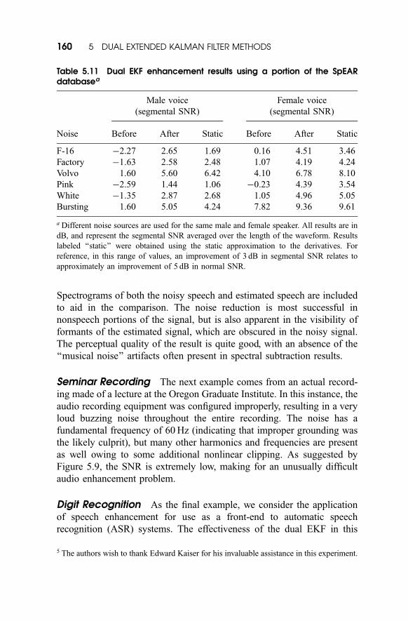
such that objective measures can still be calculated. Table 5.11 presents

sample results in terms of average segmental SNR.4

Car Phone Speech In this example, the dual EKF is used to process

an actual recording of a woman talking on her cellular telephone while

driving on the highway. The signal contains a significant level of road and

engine noise, in addition to the distortion introduced by the telephone

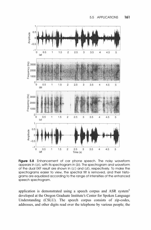
channel. The results appear in Figure 5.8, along with the noisy signal.

4 Segmental SNR is considered to be a more perceptually relevant measure than standard

SNR, and is computed as the average of the SNRs computed within 240-point windows, or

frames of speech: SSNR¼ (# frames)�1P

i max (SNRi, �10 dB). Here, SNRi is the SNR

of the ith frame (weighted by a Hanning window), which is thresholded from below at

�10 dB. The thresholding reduces the contribution of portions of the series where no

speech is present (i.e., where the SNR is strongly negative) [49], and is expected to

improve the measure’s perceptual relevance.


Spectrograms of both the noisy speech and estimated speech are included

to aid in the comparison. The noise reduction is most successful in

nonspeech portions of the signal, but is also apparent in the visibility of

formants of the estimated signal, which are obscured in the noisy signal.

The perceptual quality of the result is quite good, with an absence of the

‘‘musical noise’’ artifacts often present in spectral subtraction results.

Seminar Recording The next example comes from an actual record-

ing made of a lecture at the Oregon Graduate Institute. In this instance, the

audio recording equipment was configured improperly, resulting in a very

loud buzzing noise throughout the entire recording. The noise has a

fundamental frequency of 60 Hz (indicating that improper grounding was

the likely culprit), but many other harmonics and frequencies are present

as well owing to some additional nonlinear clipping. As suggested by

Figure 5.9, the SNR is extremely low, making for an unusually difficult

audio enhancement problem.

Digit Recognition As the final example, we consider the application

of speech enhancement for use as a front-end to automatic speech

recognition (ASR) systems. The effectiveness of the dual EKF in this

Table 5.11 Dual EKF enhancement results using a portion of the SpEARdatabasea

Male voice

(segmental SNR)

Female voice

(segmental SNR)

Noise Before After Static Before After Static

F-16 �2.27 2.65 1.69 0.16 4.51 3.46

Factory �1:63 2.58 2.48 1.07 4.19 4.24

Volvo 1.60 5.60 6.42 4.10 6.78 8.10

Pink �2.59 1.44 1.06 �0.23 4.39 3.54

White �1:35 2.87 2.68 1.05 4.96 5.05

Bursting 1.60 5.05 4.24 7.82 9.36 9.61

a Different noise sources are used for the same male and female speaker. All results are in

dB, and represent the segmental SNR averaged over the length of the waveform. Results

labeled ‘‘static’’ were obtained using the static approximation to the derivatives. For

reference, in this range of values, an improvement of 3 dB in segmental SNR relates to

approximately an improvement of 5 dB in normal SNR.

5 The authors wish to thank Edward Kaiser for his invaluable assistance in this experiment.


application is demonstrated using a speech corpus and ASR system5

developed at the Oregon Graduate Institute’s Center for Spoken Language

Understanding (CSLU). The speech corpus consists of zip-codes,

addresses, and other digits read over the telephone by various people; the

Figure 5.8 Enhancement of car phone speech. The noisy waveformappears in (a ), with its spectrogram in (b). The spectrogram and waveformof the dual EKF result are shown in (c ) and (d ), respectively. To make thespectrograms easier to view, the spectral tilt is removed, and their histo-grams are equalized according to the range of intensities of the enhancedspeech spectrogram.


ASR system is a speaker-independent digit recognizer, trained exclusively

to recognize numbers from zero to nine when read over the phone.

A subset of 599 sentences was used in this experiment. As seen in Table

5.12, the recognition rates on the clean telephone speech are quite good.

However, adding white Gaussian noise to the speech at 6 dB significantly

reduces the performance. In addition to the dual EKF, a standard spectral

subtraction routine and an enhancement algorithm built into the speech

codec TIA=EIA=IS-718 for digital cellular phones (published by the

Figure 5.9 Enhancement of high-noise seminar recording. The noisy wave-form appears in (a ), with its spectrogram in (b). The spectrogram andwaveform of the dual EKF result are shown in (c ) and (d ), respectively.


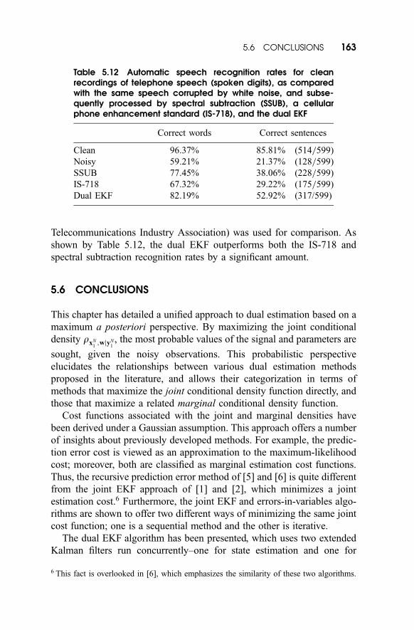
Telecommunications Industry Association) was used for comparison. As

shown by Table 5.12, the dual EKF outperforms both the IS-718 and

spectral subtraction recognition rates by a significant amount.

5.6 CONCLUSIONS

This chapter has detailed a unified approach to dual estimation based on a

maximum a posteriori perspective. By maximizing the joint conditional

density rxN1;wjyN

1, the most probable values of the signal and parameters are

sought, given the noisy observations. This probabilistic perspective

elucidates the relationships between various dual estimation methods

proposed in the literature, and allows their categorization in terms of

methods that maximize the joint conditional density function directly, and

those that maximize a related marginal conditional density function.

Cost functions associated with the joint and marginal densities have

been derived under a Gaussian assumption. This approach offers a number

of insights about previously developed methods. For example, the predic-

tion error cost is viewed as an approximation to the maximum-likelihood

cost; moreover, both are classified as marginal estimation cost functions.

Thus, the recursive prediction error method of [5] and [6] is quite different

from the joint EKF approach of [1] and [2], which minimizes a joint

estimation cost.6 Furthermore, the joint EKF and errors-in-variables algo-

rithms are shown to offer two different ways of minimizing the same joint

cost function; one is a sequential method and the other is iterative.

The dual EKF algorithm has been presented, which uses two extended

Kalman filters run concurrently–one for state estimation and one for

Table 5.12 Automatic speech recognition rates for cleanrecordings of telephone speech (spoken digits), as comparedwith the same speech corrupted by white noise, and subse-quently processed by spectral subtraction (SSUB), a cellularphone enhancement standard (IS-718), and the dual EKF

Correct words Correct sentences

Clean 96.37% 85.81% (514=599)

Noisy 59.21% 21.37% (128=599)

SSUB 77.45% 38.06% (228=599)

IS-718 67.32% 29.22% (175=599)

Dual EKF 82.19% 52.92% (317/599)

6 This fact is overlooked in [6], which emphasizes the similarity of these two algorithms.

5.6 CONCLUSIONS 163

weight estimation. By modification of the weight filter into an observed

error form, it is possible to minimize each of the cost functions that are

developed.7 This provided a common algorithmic platform for the

implementation of a broad variety of methods. In general, the dual EKF

algorithm represents a sequential approach, which is applicable to both

linear and nonlinear models, and which can be used in the presence of

white or colored measurement noise. In addition, the algorithm has been

extended to provide estimation of noise variance parameters within the

same theoretical framework; this contribution is crucial in applications for

which this information is not otherwise available.

Finally, a number of examples have been presented to illustrate the

performance of the dual EKF methods. The ability of the dual EKF to

capture the underlying dynamics of a noisy time series has been illustrated

using the chaotic Henon map. The application of the algorithm to the IP

series demonstrates its potential in a real-world prediction context. On

speech enhancement problems, the lack of musical noise in the enhanced

speech underscores the advantages of a time-domain approach; the

usefulness of the dual EKF as a front-end to a speech recognizer has

also been demonstrated. In general, the state-space formulation of the

algorithm makes it applicable to a much wider variety of contexts than has

been explored here. The intent of this chapter was to show the utility of the

dual EKF as a fundamental method for solving a range of problems in

signal processing and modeling.

ACKNOWLEDGMENTS

This work was sponsored in part by the NSF under Grants ECS-0083106

and IRI-9712346.

APPENDIX A: RECURRENT DERIVATIVE OF THE KALMAN GAIN

(1) With Respect to the Weights

In the state-estimation filter, the derivative of the Kalman gain with respect

to the weights w is computed as follows. Denoting the derivative of Kxk

7 Note that Kalman algorithms are approximate MAP optimization procedures for

nonlinear systems. Hence, future work considers alternative optimization procedures

(e.g., unscented Kalman filters [29]), which can still be cast within the same theoretically

motivated dual estimation framework.


with respect to the ith element of ww by @Kxk=@wwðiÞ (the ith column of

@Kxk=@ww) gives

@Kxk

@wwðiÞ¼

I � KxkC

CP�xk

CTþ s2

n

@P�xk

@wwðiÞCT ; ð5:109Þ

where the derivatives of the error covariances are

@P�xk

@wwðiÞ¼

@Ak�1

@wwðiÞPxk�1

ATk�1 þ Ak�1

@Pxk�1

@wwðiÞAT

k�1 þ Ak�1Pxk�1

@ATk�1

@wwðiÞ; ð5:110Þ

@Pxk�1

@wwðiÞ¼ �

@Kxk�1

@wwðiÞCP�

k�1 þ ðI � Kxk�1CÞ

@P�xk�1

@wwðiÞ: ð5:111Þ

Note that Ak�1 depends not only on the weights ww, but also on the point of

linearization, xxk�1. Therefore,

@Ak�1

@wwðiÞ¼

@2F

@xxk�1@wwðiÞþ

@2F

ð@xxk�1Þ2

@xxk�1

@wwðiÞ; ð5:112Þ

where the first term is the static derivative of Ak�1 ¼ @F=@xk�1 with xxk�1

fixed, and the second term includes the recurrent derivative of xxk�1. The

term @2F=ð@xxk�1Þ2 actually represents a three-dimensional tensor (rather

than a matrix), and care must be taken with this calculation. However,

when Ak�1 takes on a sparse structure, as with time-series applications, its

derivative with respect to x contains mostly zeroes, and is in fact entirely

zero for linear models.

(2) With Respect to the Variances

In the variance-estimation filter, the derivatives @Kxk=@s

2 may be calcu-

lated as follows:

@Kxk

@s2¼

I � KxkC

CP�k CT

þ s2n

@P�xk

@s2CT ; ð5:113Þ

APPENDIX A 165

where

@P�xk

@s2¼

@Ak�1

@s2Pk�1AT

k�1 þ Ak�1

@Pxk�1

@s2AT

k�1 þ Ak�1Pk�1

@Ak�1

@s2; ð5:114Þ

@Pxk�1

@s2¼ �

@Kxk�1

@s2CP�

k�1 þ ðI � Kxk�1CÞ

@P�xk�1

@s2: ð5:115Þ

Because Ak�1 depends on the linearization point, xxk�1, its derivative is

@Ak�1

@s2¼

@Ak�1

@xxk�1

@xxk�1

@s2; ð5:116Þ

where again the derivative @ww=@s2 is assumed to be zero.

APPENDIX B: DUAL EKF WITH COLORED MEASUREMENT NOISE

In this appendix, we give dual EKF equations for additive colored noise.

Colored noise is modeled as a linear AR process:

nk ¼PMn

i¼1

aðiÞn nk�i þ vn;k; ð5:128Þ

where the parameters aðiÞn are assumed to be known, and vnk is a white

Gaussian process with (possibly unknown) variance s2vn

. The noise nk can

now be thought of as a second signal added to the first, but with the

distinction that it has been generated by a known system. Note that the

constraint yk ¼ xk þ nk , requires that the estimates xxk and nnk must also

sum to yk . To enforce this constraint, both the signal and noise are

incorporated into a combined state-space representation:

k ¼ Fcð k�1;w; anÞ þ Bcvc;k; ð5:129Þ

xk

nk

� �¼

Fðxk�1;wÞ

An � nk�1

� �þ

B 0

0 Bn

� �vk

vn;k

� �; ð5:130Þ

yk ¼ Ccjk;

yk ¼ ½C Cn�xk

nk

� �;


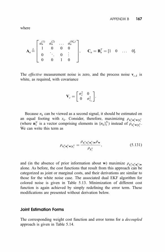
where

An ¼4

að1Þn a

ð2Þn . . . a

ðMnÞn

1 0 0 0

0 . ..

0 ...

0 0 1 0

26664

37775; Cn ¼ BT

n ¼ ½1 0 . . . 0�:

The effective measurement noise is zero, and the process noise vc;k is

white, as required, with covariance

Vc ¼s2v 0

0 s2vn

� �:

Because nk can be viewed as a second signal, it should be estimated on

an equal footing with xk . Consider, therefore, maximizing rxN1

nN1

wjyN1

(where nN1 is a vector comprising elements in fnkg

N1 ) instead of rxN

1wjyN

1.

We can write this term as

rxN1

nN1

wjyN1¼

ryN1

xN1

nN1jwrw

ryN1

; ð5:131Þ

and (in the absence of prior information about w) maximize ryN1

xN1

nN1jw

alone. As before, the cost functions that result from this approach can be

categorized as joint or marginal costs, and their derivations are similar to

those for the white noise case. The associated dual EKF algorithm for

colored noise is given in Table 5.13. Minimization of different cost

function is again achieved by simply redefining the error term. These

modifications are presented without derivation below.

Joint Estimation Forms

The corresponding weight cost function and error terms for a decoupled

approach is given in Table 5.14.

APPENDIX B 167

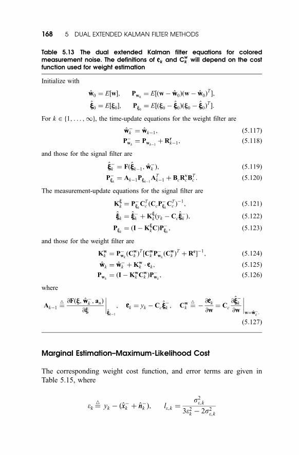
Marginal Estimation–Maximum-Likelihood Cost

The corresponding weight cost function, and error terms are given in

Table 5.15, where

ek ¼4

yk � ðxx�k þ nn�k Þ; le;k ¼s2e;k

3e2k � 2s2

e;k

Table 5.13 The dual extended Kalman filter equations for coloredmeasurement noise. The definitions of k and Cw

k will depend on the costfunction used for weight estimation

Initialize with

ww0 ¼ E½w�; Pw0¼ E½ðw � ww0Þðw � ww0Þ

T�;

jj0 ¼ E½j0�; Pj0¼ E½ðj0 � jj0Þðj0 � jj0Þ

T�:

For k 2 1; . . . ;1f g, the time-update equations for the weight filter are

ww�k ¼ wwk�1; ð5:117Þ

P�wk

¼ Pwk�1þ Rr

k�1; ð5:118Þ

and those for the signal filter are

jj�k ¼ Fðjjk�1; ww�k Þ; ð5:119Þ

P�jk¼ Ak�1Pjk�1

ATk�1 þ BcRv

cBTc : ð5:120Þ

The measurement-update equations for the signal filter are

Kjk ¼ P�

jkCT

c ðCcP�jk

CTc Þ

�1; ð5:121Þ

jjk ¼ jj�k þ Kjkðyk � Ccjj

�k Þ; ð5:122Þ

Pjk¼ ðI � K

jkCÞP�

jk; ð5:123Þ

and those for the weight filter are

Kwk ¼ P�

wkðCw

k ÞT½Cw

k P�wkðCw

k ÞTþ Re�

�1; ð5:124Þ

wwk ¼ ww�k þ Kw

k � k; ð5:125Þ

Pwk¼ ðI � Kw

k Cwk ÞP

�wk; ð5:126Þ

where

Ak�1 ¼4 @Fðj; ww�

k ; anÞ

@j

��jjk�1

; k ¼ yk � Ccjj�k ; Cw

k ¼4

�@ k

@w¼ Cc

@jj�k@w

��w¼ww�

k:

ð5:127Þ


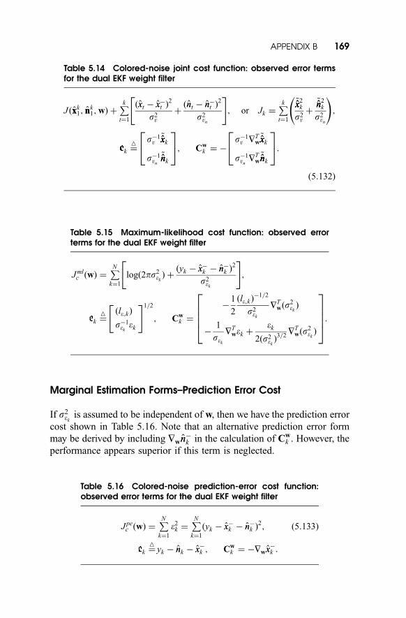
Marginal Estimation Forms–Prediction Error Cost

If s2ek

is assumed to be independent of w, then we have the prediction error

cost shown in Table 5.16. Note that an alternative prediction error form

may be derived by including Hwnn�k in the calculation of Cw

k . However, the

performance appears superior if this term is neglected.

Table 5.15 Maximum-likelihood cost function: observed errorterms for the dual EKF weight filter

J mlc ðwÞ ¼

PNk¼1

logð2ps2ekÞ þ

ðyk � xx�k � nn�k Þ

2

s2ek

" #;

k ¼4 ðle;kÞ

s�1ekek

" #1=2

; Cwk ¼

�1

2

ðle;kÞ�1=2

s2ek

HTwðs

2ekÞ

�1

sek

HTwek þ

ek

2ðs2ekÞ3=2

HTwðs

2ekÞ

26664

37775:

Table 5.16 Colored-noise prediction-error cost function:observed error terms for the dual EKF weight filter

J pec ðwÞ ¼

PNk¼1

e2k ¼

PNk¼1

ðyk � xx�k � nn�k Þ

2; ð5:133Þ

k ¼4

yk � nnk � xx�k ; Cwk ¼ �Hwxx�k :

Table 5.14 Colored-noise joint cost function: observed error termsfor the dual EKF weight filter

J ðxxk1; nnk

1;wÞ þPkt¼1

ðxxt � xx�t Þ2

s2v

þðnnt � nn�

t Þ2

s2vn

" #; or Jk ¼

Pkt¼1

~xxxx2k

s2v

þ~nnnn2

k

s2vn

!;

k ¼4

s�1v

~xxxxk

s�1vn

~nnnnk

24

35; Cw

k ¼ �s�1v HT

w~xxxxk

s�1vnHT

w~nnnnk

24

35:

ð5:132Þ

APPENDIX B 169

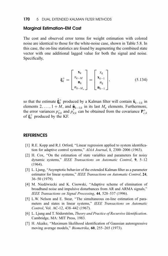
Marginal Estimation–EM Cost

The cost and observed error terms for weight estimation with colored

noise are identical to those for the white-noise case, shown in Table 5.8. In

this case, the on-line statistics are found by augmenting the combined state

vector with one additional lagged value for both the signal and noise.

Specifically,

jþk ¼

xk

xk�M

nk

nk�Mn

2664

3775 ¼

xk

xk�1

nk

nk�1

2664

3775; ð5:134Þ

so that the estimate jjþk produced by a Kalman filter will contain xxk�1jk in

elements 2; . . . ; 1 þ M , and nnk�1jk in its last Mn elements. Furthermore,

the error variances p�kjk and p

y

kjk can be obtained from the covariance Pþc;k

of jþk produced by the KF.

REFERENCES

[1] R.E. Kopp and R.J. Orford, ‘‘Linear regression applied to system identifica-

tion for adaptive control systems,’’ AIAA Journal, 1, 2300–2006 (1963).

[2] H. Cox, ‘‘On the estimation of state variables and parameters for noisy

dynamic systems,’’ IEEE Transactions on Automatic Control, 9, 5–12

(1964).

[3] L. Ljung, ‘‘Asymptotic behavior of the extended Kalman filter as a parameter

estimator for linear systems,’’ IEEE Transactions on Automatic Control, 24,

36–50 (1979).

[4] M. Niedzwiecki and K. Cisowski, ‘‘Adaptive scheme of elimination of

broadband noise and impulsive disturbances from AR and ARMA signals,’’

IEEE Transactions on Signal Processing, 44, 528–537 (1996).

[5] L.W. Nelson and E. Stear, ‘‘The simultaneous on-line estimation of para-

meters and states in linear systems,’’ IEEE Transactions on Automatic

Control, Vol. AC-12, 438–442 (1967).

[6] L. Ljung and T. Soderstrom, Theory and Practice of Recursive Identification.

Cambridge, MA: MIT Press, 1983.

[7] H. Akaike, ‘‘Maximum likelihood identification of Gaussian autoregressive

moving average models,’’ Biometrika, 60, 255–265 (1973).


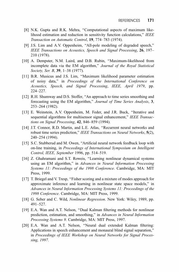
[8] N.K. Gupta and R.K. Mehra, ‘‘Computational aspects of maximum like-

lihood estimation and reduction in sensitivity function calculations,’’ IEEE

Transaction on Automatic Control, 19, 774–783 (1974).

[9] J.S. Lim and A.V. Oppenheim, ‘‘All-pole modeling of degraded speech,’’

IEEE Transactions on Acoustics, Speech and Signal Processing, 26, 197–

210 (1978).

[10] A. Dempster, N.M. Laird, and D.B. Rubin, ‘‘Maximum-likelihood from

incomplete data via the EM algorithm,’’ Journal of the Royal Statistical

Society, Ser. B, 39, 1–38 (1977).

[11] B.R. Musicus and J.S. Lim, ‘‘Maximum likelihood parameter estimation

of noisy data,’’ in Proceedings of the International Conference on

Acoustics, Speech, and Signal Processing, IEEE, April 1979, pp.

224–227.

[12] R.H. Shumway and D.S. Stoffer, ‘‘An approach to time series smoothing and

forecasting using the EM algorithm,’’ Journal of Time Series Analysis, 3,

253–264 (1982).

[13] E. Weinstein, A.V. Oppenheim, M. Feder, and J.R. Buck, ‘‘Iterative and

sequential algorithms for multisensor signal enhancement,’’ IEEE Transac-

tions on Signal Processing, 42, 846–859 (1994).

[14] J.T. Connor, R.D. Martin, and L.E. Atlas, ‘‘Recurrent neural networks and

robust time series prediction,’’ IEEE Transactions on Neural Networks, 5(2),

240–254 (1994).

[15] S.C. Stubberud and M. Owen, ‘‘Artificial neural network feedback loop with

on-line training, in Proceedings of International Symposium on Intelligent

Control, IEEE, September 1996, pp. 514–519.

[16] Z. Ghahramani and S.T. Roweis, ‘‘Learning nonlinear dynamical systems

using an EM algorithm,’’ in Advances in Neural Information Processing

Systems 11: Proceedings of the 1998 Conference. Cambridge, MA: MIT

Press, 1999.

[17] T. Briegel and V. Tresp, ‘‘Fisher scoring and a mixture of modes approach for

approximate inference and learning in nonlinear state space models,’’ in

Advances in Neural Information Processing Systems 11: Proceedings of the

1998 Conference. Cambridge, MA: MIT Press, 1999.

[18] G. Seber and C. Wild, Nonlinear Regression. New York: Wiley, 1989, pp.

491–527.

[19] E.A. Wan and A.T. Nelson, ‘‘Dual Kalman filtering methods for nonlinear

prediction, estimation, and smoothing,’’ in Advances in Neural Information

Processing Systems 9. Cambridge, MA: MIT Press, 1997.

[20] E.A. Wan and A.T. Nelson, ‘‘Neural dual extended Kalman filtering:

Applications in speech enhancement and monaural blind signal separation,’’

in Proceedings of IEEE Workshop on Neural Networks for Signal Proces-

sing, 1997.

REFERENCES 171

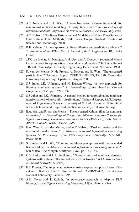
[21] A.T. Nelson and E.A. Wan, ‘‘A two-observation Kalman framework for

maximum-likelihood modeling of noisy time series,’’ in Proceedings of

International Joint Conference on Neural Networks, IEEE/INNS, May 1998.

[22] A.T. Nelson, ‘‘Nonlinear Estimation and Modeling of Noisy Time-Series by

Dual Kalman Filter Methods,’’ PhD thesis, Oregon Graduate Institute of

Science and Technology, 2000.

[23] R.E. Kalman, ‘‘A new approach to linear filtering and prediction problems,’’

Transactions of the ASME, Ser. D, Journal of Basic Engineering, 82, 35–45

(1960).

[24] J.F.G. de Freitas, M. Niranjan, A.H. Gee, and A. Doucet, ‘‘Sequential Monte

Carlo methods for optimisation of neural network models,’’ Technical Report

TR-328, Cambridge University Engineering Department, November 1998.

[25] R. van der Merwe, N. de Freitas, A. Doucet, and E. Wan, ‘‘The unscented

particle filter,’’ Technical Report CUED=F-INFENG=TR 380, Cambridge

University Engineering Department, August 2000.

[26] S.J. Julier, J.K. Uhlmann, and H. Durrant-Whyte, ‘‘A new approach for

filtering nonlinear systems,’’ in Proceedings of the American Control

Conference, 1995, pp. 1628–1632.

[27] S.J. Julier and J.K. Uhlmann, ‘‘A general method for approximating nonlinear

transformations of probability distributions,’’ Technical Report, RRG, Depart-

ment of Engineering Science, University of Oxford, November 1996. http://

www.robots.ox.ac.uk/~siju/work/publications/letter_size/Unscented.zip.

[28] E.A. Wan and R. van der Merwe, ‘‘The unscented Kalman filter for nonlinear

estimation,’’ in Proceedings of Symposium 2000 on Adaptive Systems for

Signal Processing, Communication and Control (AS-SPCC), Lake Louise,

Alberta, Canada, IEEE, October 2000.

[29] E.A. Wan, R. van der Merwe, and A.T. Nelson, ‘‘Dual estimation and the

unscented transformation,’’ in Advances in Neural Information Processing

Systems 12: Proceedings of the 1999 Conference. Cambridge, MA: MIT

Press, 2000.

[30] S. Singhal and L. Wu, ‘‘Training multilayer perceptrons with the extended

Kalman filter,’’ in Advances in Neural Information Processing Systems 1.

San Mateo, CA: Morgan Kauffman, 1989, pp. 133–140.

[31] G.V. Puskorius and L.A. Feldkamp, ‘‘Neural control of nonlinear dynamic

systems with Kalman filter trained recurrent networks,’’ IEEE Transactions

on Neural Networks, 5 (1994).

[32] E.S. Plumer, ‘‘Training neural networks using sequential-update forms of the

extended Kalman filter,’’ Informal Report LA-UR-95-422, Los Alamos

National Laboratory, January 1995.

[33] A.H. Sayed and T. Kailath, ‘‘A state-space approach to adaptive RLS

filtering,’’ IEEE Signal Processing Magazine, 11(3), 18–60 (1994).


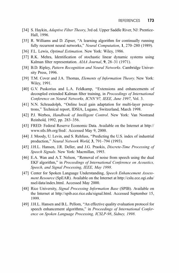
[34] S. Haykin, Adaptive Filter Theory, 3rd ed. Upper Saddle River, NJ: Prentice-

Hall, 1996.

[35] R. Williams and D. Zipser, ‘‘A learning algorithm for continually running

fully recurrent neural networks,’’ Neural Computation, 1, 270–280 (1989).

[36] F.L. Lewis, Optimal Estimation. New York: Wiley, 1986.

[37] R.K. Mehra, Identification of stochastic linear dynamic systems using

Kalman filter representation. AIAA Journal, 9, 28–31 (1971).

[38] B.D. Ripley, Pattern Recognition and Neural Networks. Cambridge Univer-

sity Press, 1996.

[39] T.M. Cover and J.A. Thomas, Elements of Information Theory. New York:

Wiley, 1991.

[40] G.V. Puskorius and L.A. Feldkamp, ‘‘Extensions and enhancements of

decoupled extended Kalman filter training, in Proceedings of International

Conference on Neural Networks, ICNN’97, IEEE, June 1997, Vol. 3.

[41] N.N. Schraudolph, ‘‘Online local gain adaptation for multi-layer percep-

trons,’’ Technical report, IDSIA, Lugano, Switzerland, March 1998.

[42] P.J. Werbos, Handbook of Intelligent Control. New York: Van Nostrand

Reinhold, 1992, pp. 283–356.

[43] FRED: Federal Reserve Economic Data. Available on the Internet at http://

www.stls.frb.org/fred/. Accessed May 9, 2000.

[44] J. Moody, U. Levin, and S. Rehfuss, ‘‘Predicting the U.S. index of industrial

production,’’ Neural Network World, 3, 791–794 (1993).

[45] J.H.L. Hansen, J.R. Deller, and J.G. Praokis, Discrete-Time Processing of

Speech Signals. New York: Macmillan, 1993.

[46] E.A. Wan and A.T. Nelson, ‘‘Removal of noise from speech using the dual

EKF algorithm,’’ in Proceedings of International Conference on Acoustics,

Speech, and Signal Processing, IEEE, May 1998.

[47] Center for Spoken Language Understanding, Speech Enhancement Assess-

ment Resource (SpEAR). Available on the Internet at http://cslu.ece.ogi.edu/

nsel/data/index.html. Accessed May 2000.

[48] Rice University, Signal Processing Information Base (SPIB). Available on

the Internet at http://spib.ece.rice.edu/signal.html. Accessed September 15,

1999.

[49] J.H.L. Hansen and B.L. Pellom, ‘‘An effective quality evaluation protocol for

speech enhancement algorithms,’’ in Proceedings of International Confer-

ence on Spoken Language Processing, ICSLP-98, Sidney, 1998.

REFERENCES 173

Documents

DUAL EXTENDED KALMAN FILTER METHODS - pudn.comread.pudn.com/downloads142/ebook/620455/Kalman... · Kalman Filtering and Neural Networks, Edited by Simon Haykin ISBN 0-471-36998-5