Dual-Pump CARS Measurements in the University of Virginia ... · American Institute of Aeronautics and Astronautics 1 Dual-Pump CARS Measurements in the University of Virginia's Dual-Mode

American Institute of Aeronautics and Astronautics

1

Dual-Pump CARS Measurements in the University of Virginia's Dual-Mode Scramjet: Configuration “C”

Andrew D. Cutler*, Gaetano Magnotti†, Luca Cantu†, Emanuela Gallo† The George Washington University, Mechanical and Aerospace Engineering,

1 Old Oyster Point Road, Suite 200, Newport News, VA, 23602

Paul M. Danehy‡ NASA Langley Research Center, Hampton, VA, 23681

Robert Rockwell§, Christopher Goyne**, and Jim McDaniel††

University of Virginia, Mechanical and Aerospace Engineering, Charlottesville, VA 22904

Measurements have been conducted at the University of Virginia Supersonic Combustion Facility in configuration C of the dual-mode scramjet. This is a continuation of previously published works on configuration A. The scramjet is hydrogen fueled and operated at two equivalence ratios, one representative of the “scram” mode and the other of the “ram” mode. Dual-pump CARS was used to acquire the mole fractions of the major species as well as the rotational and vibrational temperatures of N2. Developments in methods and uncertainties in fitting CARS spectra for vibrational temperature are discussed. Mean quantities and the standard deviation of the turbulent fluctuations at multiple planes in the flow path are presented. In the “scram” case the combustion of fuel is completed before the end of the measurement domain, while for the ram case the measurement domain extends into the region where the flow is accelerating and combustion is almost completed. Higher vibrational than rotational temperature is observed in those parts of the hot combustion plume where there is substantial H2 (and hence chemical reaction) present.

I. Introduction Under the auspices of the National Center for Hypersonic Combined Cycle Propulsion1 a series of dual-mode

scramjet experiments are being conducted at the University of Virginia. The aim of these experiments is to examine the flow processes that take place in the isolator and combustor of a direct-connect scramjet model that is operated at flight enthalpy of Mach 5, and to obtain benchmark data sets in order to validate numerical models. The scramjet combustor has optical access suitable for the application of advanced optical measurements techniques, while long duration testing capability allows large data sets to be built up at a fixed test point, and point statistics of the flow variables to converge. The diagnostics are aimed at capturing the physics of turbulent reacting flows and many of the measurement techniques are spatially and temporally resolved. In particular, statistics of the turbulent flow are being measured using dual-pump CARS.

Coherent anti-Stokes Raman spectroscopy (CARS) is a non-linear spectroscopic technique in which three laser beams, two pump beams (with frequencies ωp1 and ωp2) and a Stokes beam (ωS), are focused and crossed at their focal point, and a fourth signal laser beam (ωa-S) is generated at the intersection through a four-wave mixing process. Resonances associated with Raman active molecular rotational-vibrational transitions strengthen the CARS signal in a manner dependent on gas composition and temperature. The wavelength of excitation or “Raman shift” corresponds to the difference in energy between a pump beam and a Stokes beam (longer wavelength) photon. In the broadband CARS technique one of the laser beams, the Stokes beam, is spectrally broad whereas the other pump beams are spectrally narrow, and this enables multiple resonances to be excited simultaneously. The signal is

* Professor. Associate Fellow AIAA † Graduate student. Member AIAA ‡ Research Scientist. Associate Fellow AIAA § Senior Scientist. Member AIAA ** Research Associate Professor, Associate Fellow AIAA †† Professor, Associate Fellow AIAA

https://ntrs.nasa.gov/search.jsp?R=20130003230 2019-08-19T18:23:30+00:00Z


2

spectrally broad and carries with it the spectral signature of the gases present (over some range of wavelengths). It is dispersed by a spectrometer and spectra are compared to theoretical models to obtain information on composition and temperature. In dual-pump CARS, originally developed by Lucht and coworkers,2,3

the two pump beams are at different wavelengths and two different ranges of Raman shift may be excited. The energy level diagram for one of the CARS processes is illustrated in Figure 1(a) while in the second CARS process the roles of the pump beams are swapped. A planar BOXCARS configuration (Figure 1b) is adopted in which the Stokes and one of the pump beams are nearly collinear and the signal beam is emitted nearly collinear with the other pump. The CARS method employed in this work is based on the techniques developed at NASA Langley4,5,6,7 and is described by Magnotti.8

(a) (b)

Figure 1. Dual-pump CARS: (a) energy level diagram, (b) beam crossing geometry.

Previously we have reported on an extensive CARS data base acquired in configuration “A” of the scramjet.9,10 Computations of this flow field using Reynolds-averaged Navier-Stokes and large eddy simulation methods and comparisons to the configuration A CARS measurements are reported in Ref. 11. In this latest work we report on a similar CARS data base acquired in configuration “C”. The latter configuration differs from the former in two respects. Firstly, a constant area section of duct or “isolator” is placed between the nozzle exit and the combustor. This change allows the combustor to operate in both modes of a dual-mode scramjet: the “scram” mode where the flow entering the combustor is supersonic, and remains supersonic (in the one dimensional sense) throughout; and the “ram” mode where the pressure rise in the combustor propagates upstream into the isolator, leading to subsonic flow at the entrance to the combustor and a thermal throat towards the end. Secondly, a short constant area section of duct is placed between the combustor and the extension to the combustor. In Ref. 12 we reported on CARS measurements at the entrance plane of the combustor for both configurations A and C and these showed that the N2 (and to a lesser extent the O2) entering the combustor was not in vibrational equilibrium, but that the N2 vibrational temperature was equal to the temperature in the facility heater while the rotational temperature was much cooler. This non-equilibrium was present even for configuration C where the entrance plane was further downstream (after the inlet isolator). These results compared well with existing computational models. In the present work a new technique for fitting the CARS spectra for vibrational temperature of N2 is reported, as are extensive measurements of this parameter in the combustor.

II. Test Facility and Dual-Mode Scramjet

A. Experiment The experiment was conducted using the University of Virginia Supersonic Combustion Facility (UVaSCF).13,14

This facility is an electrically heated, continuous flow scramjet wind tunnel that is operated in direct-connect mode. It is capable of simulating Mach 5 flight enthalpy and provides a clean test flow of air that is free of contaminants (such as those from combustion vitiation or arc-heated facilities). Facility run times of the order of five hours or more are possible and, because of good optical access and proximity to laser diagnostics labs, the facility is well suited to the application of advanced instream diagnostics such as CARS. Figure 2 presents a schematic of the dual-mode scramjet flow path that was used for the CARS measurements. (Although the schematic shows the flow path horizontal, it is vertical.) The flow path consists of a Mach 2 facility nozzle directly coupled to an isolator duct that is 25.4 mm × 38.1 mm (1” × 1.5”) in cross section and 266 mm long. The exit of the isolator is connected to the combustor. One of the walls of the combustor houses a ramp fuel injector through which hydrogen fuel is injected. The ramp is 12.7 mm (0.5”) wide and the forward face is angled 10° to the injector wall. The injector-surface-normal height H is 6.35 mm (0.25”); this height is used to non-dimensionalize the spatial variables. Fuel injection takes place through a conical Mach 1.7 nozzle at the base of the ramp with its main

Rotational-vibrational states

Virtual statesωp1

ωS

ωp2

ωa-S Measurement volume

Signal beamLens


3

axis parallel to the ramp face. All walls in the flow path are parallel except for the wall that houses the fuel injector. This wall diverges at a 2.9° angle to the opposite wall beginning at the leading edge of the ramp fuel injector. The divergence results in the ramp face having an angle of incidence to the incoming flow of 7.1°. At the end of the isolator is a 149 mm long constant area section. The 2.9° divergence continues through the 180 mm long extender duct and terminates with an atmospheric backpressure at the exit. All components in the flow path are made of stainless steel and the walls in the combustor section, including the ramp, are coated in a 0.38 mm thick layer of thermal barrier zirconia. The wall that houses the fuel injector is instrumented with low frequency pressure taps that are mostly aligned on the combustor centerline. Type K thermocouples are also located in the wall along the centerline at six axial stations downstream of fuel injection. Reference 9 provides further details on the flow path and instrumentation. The five CARS measurement planes that were used in this study are presented in Figure 2. The planes were at x/H=-10.3, 6.1, 18.1, 38, and 56.1 (denoted Planes 0, 1, 2, 3, and 4 respectively) relative to the point of fuel injection. Measurements at Plane 0 (the entrance plane) were intended to quantify the upstream boundary condition in the combustor, while the four downstream planes enable interrogation of the fuel-air mixing and combustion zone downstream of fuel injection. To enable CARS measurements, the two side walls of the flow path each incorporated a 3.18 mm wide slot that spanned the entire height of the duct at each plane. When measurements were not conducted at a particular plane, the slots were filled with a stainless steel plug. The active slots were sealed from the atmosphere using an arrangement that offset the windows away from the flow path by 127 mm (to avoid damage by the focused laser beams) and purged by a small flow of air.

Figure 2. Dual-mode scramjet flowpath used for CARS measurements; CARS measurement planes marked 0 to 4. Temperature contours are shown at the measurement planes in the bottom view.

Data acquisition for the scramjet flow path parameters was performed using a NetScannerTM pressure scanner that was operated with a remote NetScannerTM thermocouple unit. Typically a scan of 20 samples was acquired over 2 seconds at a sample rate of 10 Hz for each pressure tap and thermocouple. Quantities for each tap or thermocouple were then averaged prior to plotting. Pressure and temperature were typically measured to within ±0.5% and average quantities typically had a 95% confidence interval of no more than ±1.5%. As presented in Table 1, the scramjet flowpath was fueled at equivalence ratios of 0.18 and 0.49. The fuel-air mixture in the combustor autoignited at an equivalence ratio of approximately 0.14 and combustion was self sustaining following ignition.

Mach 2 nozzle Fuel injector CARS measurement plane

0 1 2 3 4

Isolator ConstantArea

Combustor ExtenderFacility

AirHeater

xz

y


4

Table 1 Test conditions for air flow and hydrogen fuel

Parameter Air Fuel Case 1

Fuel Case 2

Error

Total pressure (kPa) 300 465 1260 3% Total temperature (K) 1200 300 300 3% Mach numbera 2.03 1.70 1.70 Static pressurea (kPa) 37 94 255 Static temperaturea (K) 706 190 190 Equivalence ratio 0.18 0.49 5%

a Property at nozzle exit determined using nozzle area ratio and assuming isentropic flow (γ=1.34 for air and 1.40 for hydrogen).

B. Pressure Distributions Typical averaged pressures measured along the scramjet flowpath are presented in Figure 3. Pressure

distributions are shown for the cases of fuel off and fuel-air reacting at equivalence ratios, φ, of 0.18 and 0.49. Axial distances have been normalized by the normal height of the ramp and are referenced to the point of fuel injection while pressures are normalized by the pressure at the most upstream axial station (35 kPa). Referring first to the fuel off distribution, the presence of the ramp results in an oblique shock wave that is evident at x/H=-6, followed by an expansion at the base of the ramp. These waves extend downstream in the supersonic flow, reflecting back and forth from the walls of the duct. From x/H=41 to the exit of the extender at x/H=81 the pressure rises due to the 1 atmosphere backpressure on the flowpath and associated shock train and boundary layer separations. It can be seen at both equivalence ratios that combustion leads to a significant pressure increase in the scramjet flow path which must be accompanied by a reduction in Mach number. At an equivalence ratio of 0.18 the combustion-induced pressure rise extends upstream only to the ramp fuel injector. This mode of operation is referred to as the scram mode where the inflow (just upstream of the ramp) is supersonic and the flow downstream is a mixture of supersonic and subsonic. Since the inflow is supersonic there is still a shock generated pressure rise due to the ramp at x/H=-6. The pressure within the combustor is relatively constant until x/H=53, after which the pressure rises due the influence of the atmosphere backpressure at the exit. At the equivalence ratio of 0.49 it can be seen that back pressure due to combustion generates a pressure rise and shock train in the isolator starting at x/H=-33. In this case the flow entering the combustor is subsonic but the flow reaccelerates to supersonic speeds in15 between x/H =2 and 56, as evidenced by the decreasing pressure. After x/H=56 the pressure rises due the influence of the 1 atmosphere backpressure at the exit.

Figure 3. Wall pressure distributions for the two fuel-air reacting cases and also for the fuel-off case.

III. CARS Method

A. Optical System The optical system was described previously in Ref. 10, but this description is repeated herein for completeness.

The optical system, illustrated in Figure 4, consists of a mobile laser cart (not shown) located in a room adjacent to

0

0.5

1

1.5

2

2.5

3

3.5

4

4.5

-60 -50 -40 -30 -20 -10 0 10 20 30 40 50 60 70 80

No

rma

lize

d W

all

Pre

ss

ure

(p/p

ref)

Normalized Axial Distance from Fuel Injection (x/H)

φ = 0.00φ = 0.49φ = 0.18Plane 0Plane 1Plane 2Plane 3Plane 4


5

the scramjet lab, and components located in the scramjet lab. Mirrors relay the laser beams to a stepping-motor driven beam translation system, upon which transmission optics (on one board) and collection optics (on a second board) are mounted. These components are mounted on a large optical table adjacent to the facility. The laser cart contains an injection seeded Nd:YAG laser, frequency doubled to 532 nm, a portion of which is split off to form one of the pump beams. The second pump beam is a narrow band dye laser (Spectra Physics PDL-2) centered at around 550.5 nm, and the Stokes beam is a home-built broadband dye laser centered at 603 nm with FWHM of 10 nm. Both dye lasers are pumped by the Nd:YAG. The pulse width of the laser is 8 ns and the repetition rate is 20 Hz. The second pump and Stokes laser beams are collinearly overlapped at the laser cart. The cart also contains spherical-lens telescopes for controlling beam size and divergence, and a rotatable half-wave plate and polarizing beam cube combination that allows the energy of the Nd:YAG laser beam to be controlled. Laser energies at the measurement volume were typically roughly 62, 32 and 19 mJ for the Nd:YAG, the narrowband and the broadband dye laser respectively.

Figure 4. Optical system located in the scramjet lab.

Figure 5. Transmission and collection optics.

Located on the transmission board, shown in Figure 5, are mirrors that cross the Nd:YAG and overlapped dye laser beams (crossing angle of 3.9°), a 750 mm lens for focusing the dye laser beams, and a 600 mm lens for focusing the Nd:YAG. The latter lens is tilted with respect to the incoming beam so that, by introducing astigmatism, it shapes the focal spot at the beam crossing to a roughly 4:1 axis ratio ellipse with major axis orthogonal to the plane formed by the three laser beams. This helps in reducing beam steering effects in flows with large, unsteady density gradients.16 The focal length of the two lenses is long enough to ensure that laser irradiances are below the Stark broadening and stimulated Raman pumping thresholds determined in Ref. 7. The measurement volume formed by the beams intersection is roughly 1.5 mm – 2 mm long and 50 μm in diameter. A focal plane imaging system (FPI) is used to view the beams in cross-section at the crossing plane.17 A splitter (uncoated wedged glass plate) is located

Collection optics

50 mm lens

Filters, polarizer

Y-motion

Spectrometer & detector

Laser beams from the cart

Z-motion

X-motion

Signal beam

CARS windows

Transmission optics

Dual-mode scramjet

Transmission Optics Collection Optics

Dual-mode scramjet

Iris

60 cm lens

Polarizer

Signal beam

FPI Camera

75 cm lens

FPI Camera

60 cm lens Dichroic mirrors

Window boxMeasurementvolume

Laser beams from cart

Signal

Splitter

Lens & filters


6

after the focusing lenses, and directs a small fraction of the beams energy towards a secondary beam intersection. A microscope objective lens, filters, and a CCD camera are used to detect the image. This FPI system is used to set the focus, lens twist, and location of the beams at the crossing plane. The wedged glass plate is removed during data acquisition. Located on the collection optics board is a 600 mm collimating lens, a series of dichroic mirrors that reflect and separate the signal while transmitting the Nd:YAG beam upon which it is superimposed. A second FPI system is placed on this board, which uses a splitter and an achromatic lens to focus and cross the beams in front of a camera. The second system is used to monitor and realign the beams during a test. The signal is relayed back to the optical table through filters that remove remaining Nd:YAG light, a polarizer, and a spherical lens that focuses the signal at the entrance plane of a 1 m spectrometer with 2400 lines per mm grating. The slit of the spectrometer is opened wide enough to accommodate small motions of the signal focus at the entrance plane. The resolution of the system is determined by the size of the focus (as well as the spectral width of the probe beam) rather than the width of the slit aperture. The horizontally dispersed signal is recorded at the exit plane by an unintensified, scientific-grade, back-illuminated CCD camera. The pixels of the camera are binned into 3 bins vertically × 1340 pixels horizontally; the CARS signal is focused on the center bin. For additional details, see Magnotti et al.8

B. Analysis of CARS Spectra The measured spectra are preprocessed to obtain the CARS susceptibility spectra and fitted to theoretical spectra

to obtain temperature and composition as parameters of the fit. The preprocessing consists of first subtracting the background from the spectra, consisting of the instrument baseline signal level plus the signal associated with any contaminating light source, such as non-CARS emission from the flow field or room light. The background is taken to be the signal measured in bins 1 and/or 3 of the CCD, above and below the bin where the signal is located (bin 2). Every 20 laser shots the laser is not Q-switched and no CARS signal is generated; these shots are used to correct for interferences in the signal bin not present in bins 1 and 3. The spectrum is then normalized by a reference spectrum to remove the effect of the Stokes laser spectrum. The reference spectrum is acquired in a flow of argon gas, which has no resonances. The wavenumber at each pixel is computed based on previous calibration. Argon spectra were acquired immediately before and after the CARS measurements in the scramjet by moving the measurement volume outside the scramjet duct and into the argon jet. Two hundred single shot spectra were acquired, the background was subtracted, and the spectra were averaged. The reference spectra was found by interpolating from the before and the after averaged argon spectra. It is typical that the argon spectra obtained before and after differ significantly. It is also typical that this normalization does not always fully account for the effect of the Stokes laser spectrum. Recent measurements indicate that the spectrum of the Stokes laser is not spatially uniform. Figure 6 shows the CARS argon spectrum acquired as various parts of the same Stokes laser beam are blocked at the laser cart. Counts (intensity) are plotted as a function of pixel number (wavelength). As indicated in (c), A has no blocking, B the beam is reduced to about 2 mm in diameter by an iris, while C, D, G, and H are blocked at left and right by varying amounts. The measured signal counts are shown in (a); note the logarithmic coordinate and the large variation in amplitude of the CARS signal. In (b) the spectra of (a) are normalized to their respective peaks. The effect of blocking part of the beam is a shift in wavelength of the peak of the spectrum, while the shape (width at half maximum) is relatively constant. Such shifts have always been observed by us between “before” and “after” spectra, and were attributed to such factors as changes in the alignment of the Stokes laser cavity over time, changes in temperature of the dye, and so on. While these factors may play a role, it seems likely that the alignment of the CARS intersection is also important. For example, if for one argon spectra the center of the Stokes beam intersects the center of the pump/probe beams, while for another only the edge of the Stokes beam intersects them, it is expected that the spectra would be different. When this effect is coupled with the known beam steering and changes in the quality of the beams focus that occurs due to unsteady density gradients in the reacting fuel jet plume, and due to the windows of the combustor, it may be expected that the appropriate reference spectrum varies from point to point in the flow as the laser is scanned, and even from shot to shot as the flow changes due to turbulence.


7

(a) (b) (c)

Figure 6 Argon spectra as various parts of the broad band (Stokes) dye laser beam are blocked: (a) Detector counts, (b) detector counts normalized to the peak, (c) sketch indicating which part of the beam is blocked.

Beam steering by unsteady flow is illustrated in Figure 7 which contains several single laser shot images obtained over a period of time of less than one second by the second FPI. The images were acquired with the measurement volume at Plane 0 of the scramjet operating at φ=0.49. The flow was unsteady in this example due to the unsteady shock system propagating from the isolator. Each image shows a reconstruction of a cross section of the beams at a plane close to the beam intersection. The beams are in a horizontal plane. The red Stokes beam and the yellow probe/pump are overlapped (though not perfectly). The green is elliptical. The beams were set up to cross at a different axial plane than is being imaged (i.e., at a small distance perpendicular to the plane of these images). The FPI system does not exactly reconstruct what happens at the beam crossing since the beams pass through additional hot gases and suffer additional refraction in traveling from the intersection to the FPI system, so that unsteadiness of the beams at the intersection is not as bad as appears in the images. As the beams move from left to right, the intersection occurs at slightly different axial locations and as the beams move up and down the center of the red/yellow beams intersects the elliptical green at a different height.

Figure 7 Several images acquired closely together in time by the second focal plane imaging system with the measurement volume at Plane 0 with φ=0.49.

A typical example of the effect of the “shift” in the Stokes spectrum is illustrated in Figure 8, along with a fitted theoretical spectrum. This measured spectrum (average of 200 shots) is also shown in Figure 10(a) and discussed in section IV(a) The spectrum has not been corrected for a “shift” of the Stokes spectrum to the right, as shown in Figure 6(b). The result is that the experiment is high to the left and low to the right. The typical deviation shown here is quite modest and is not a large as might first be expected based on the large shifts of the argon spectra shown in Figure 6(b). Indeed, if only the three argon spectra with the highest peak counts are considered (A,B,C) then the shifts are much less - generally the CARS system is aligned to near peak CARS signal counts, so the alignments of A,B,C must be considered more typical.

1

10

100

1000

10000

0 500 1000 1500

Co

un

ts

Pixel number

A

B

C

D

G

H

0

0.1

0.2

0.3

0.4

0.5

0.6

0.7

0.8

0.9

1

0 500 1000 1500

Co

un

ts n

orm

aliz

ed t

o p

eak

Pixel number

A

B

D

C

Laser beam

H

G

Beam block

532 nm pump/probe

Yellow pump/probe

Stokes


8

Figure 8. Experimental and theoretical CARS spectra showing effect of error in reference spectrum.

Ideally, the Stokes laser would be designed to be uniform in spectral properties. The approach adopted to correct for the shifts in the Stokes laser is to add new parameters to the fit. If such measures are not adopted, then errors occur in the fitted temperature and species mole fraction. Errors are typically largest in the mole fraction of H2 since the dominant H2 line is the S(5) line which lies at the left of the spectrum where the errors in the reference spectrum (as a percentage) are largest.

C. Fitting Algorithm Theoretical spectra are calculated using the Sandia CARSFT code18, which was modified by Lucht3 for dual-

pump CARS, further modified by O’Byrne5, and modified by us to permit the calculation of spectra with different rotational and vibrational temperatures of N2 and O2.

12 The N2 and O2 Q-branches and several H2 rotational lines are resonant in our spectra. The remaining major species in H2-air combustion is H2O which is not resonant but can be estimated by difference. The N2 and O2 were modeled with the Voigt line shape model while the Galatry model with variable narrowing parameter was used for H2.

8,19 The second pump frequency offset was 633.25 cm-1. Spectra are presented as a function of signal frequency minus the second pump frequency (ωa-S - ωp2) in units of wavenumber (cm-1). Although the shapes of the spectra are fitted rather than the signal intensity, pressure affects the measurements indirectly through the line shape models. Pressure at a measurement plane was taken to be the pressure at the wall, interpolated from the pressure tap measurements. Spatial variations in pressure within a plane produce some uncertainty in the CARS measurements, primarily in the species mole fractions. It is impractical, employing libraries, to vary pressure within a plane, even if the distribution of pressure were known. The fitting code employs a library of previously calculated theoretical spectra. It has two essential features: an algorithm for interpolating theoretical spectra from the library for arbitrary values of temperature and composition, and a fitter which repeatedly calls the interpolator, minimizing the residual (the error between measured and theoretical spectra). The library is “sparsely” structured so that even for several resonant species it is not too large. The aim is a technique which interpolates spectra from the sparse library with the accuracy of interpolating from a fully packed library. Thus, it is quicker to generate, easier to manage, and the fitting algorithm is computationally faster. The method has been previously described.6 Its accuracy depends on the resonances of each species generally not overlapping. It consists of a multidimensional grid of temperatures and compositions at each of which a complete (spanning the full range of wavelength) theoretical spectrum has been calculated. The grid structure is sparse in the composition variables and the structure is repeated at every temperature value. Suppose the number of grid points in the sparse directions is 3 and in the fine direction is 10 (typical values), and there are 4 resonant species. At each temperature there are 4 sub-libraries covering the same range of compositions in regular grids of dimension 3×3×3×10, 3×3×10×3, 3×10×3×3, and 10×3×3×3, where the 4 dimensions pertain to the 4 composition variables. The resulting library is smaller than the fully packed library of dimension 10×10×10×10 by a factor of 9.3 (this factor is higher for more species). In interpolating to a specified composition at a library temperature, four spectra are interpolated, one from each sub-library at that level. Interpolation from, for example, the sub-library that has 10 points in the N2 direction is most accurate at wavelengths where N2 is resonant. The four spectra are combined to form a spectrum accurate at all wavelengths by taking a weighted sum, where the weight function multiplying each spectrum picks out the portion of the spectrum which is most accurate. Interpolation to an intermediate temperature

0

0.2

0.4

0.6

0.8

1

1.2

1.4

1.6

1.8

2

2075 2125 2175 2225 2275 2325 2375

sqrt

(No

rmal

ized

in

ten

sity

)Wave number, cm-1

Theory

Experiment


9

is by interpolation to the specified composition as just described at each of the 3 or 4 nearest temperature levels, and then interpolating between these levels. All interpolations are by means of Lagrange polynomial fits. For greatest accuracy the library spectra are constructed so that the baseline (non-resonant) susceptibility level is always 1 and only resonances associated with one molecular species in the spectrum varies at a time. Spectra are normalized by mixture non-resonant susceptibility. In order to avoid changes in the fraction of one species affecting the rest of the spectrum (through the mixture non-resonant susceptibility) the independent composition variables of the library are the species non-resonant susceptibility weighted mole fractions (ηi where i is the species index).6 Our library method has been adapted to the separate fitting of rotational and vibrational temperature of N2.

12 Two N2 pseudo-species which sum to the total of the N2 present are defined and included in the library. These species isolate signal in the first band in the N2 Q-branch from signal in the higher bands. This first band is associated with transition between the ground vibrational state (v=0) and the 1st excited vibrational state (v=1), and for given (rotational) temperature depends upon the difference in the population between these states. Thus, the first N2 species is defined to have mole fraction xN2,1 = xv=0 - xv>0, where xv=0 is the mole fraction of the mixture that is N2 in the v=0 state and xv>0 is the mole fraction of mixture in the v=1 and higher states. The second N2 species is defined xN2,2=2xv>0 . Thus the sum xN2,1 + xN2,2 equals the mole fraction of N2. Figure 9 shows several typical library spectra computed with greater probe line width than typical in our experiment (so that details of the rotational band structure do not obscure the differences) at T=1500 K. In (a) ηN2,1=0.28 while in one set of lines ηN2,2=0 and ηO2 is varied from 0 to 0.20, while in another ηN2,2 is varied from 0 to 0.35 and ηO2=0. This figure illustrates how only the region of the spectra associated with a particular species varies, while the rest is held constant. In (b) ηN2,1 is varied from 0 to 0.81 while ηN2,2=0.12 and ηO2=0 (this is a close-up in the vicinity of the N2 spectrum). Unfortunately, at this temperature, the higher rotational levels of the first band overlap the lower levels of the second band (associated with v=1 to v=2 transitions). Although the decoupling between two N2 pseudo-species is not complete, the resulting accuracy of interpolation is sufficient for the present purposes. The procedure for generating inputs to the calculation of the spectra is first to specify the η values of the library grid, second compute the corresponding mole fractions of each species (or pseudo-species), third compute the mole fraction of N2 as xN2,1 + xN2,2, and fourth compute the vibrational temperature from the fraction in the ground state which is (xN2,1 + 0.5xN2,2)/ (xN2,1 + xN2,2) assuming a Boltzmann distribution.20 The vibrational energy level calculations were the same as employed internally by the CARSFT code. This procedure is reversed in recovering vibrational temperature after fitting for the ηi’s.

(a) (b)

Figure 9. Selected library spectra in which (a) ηN2,1 and either ηN2,2 or ηO2 is held constant while the other is varied, (b) ηO2 and ηN2,2 is held constant while ηN2,1 is varied.

The fitting algorithm minimizes the following residual:6 1

0

1

2

3

4

5

6

7

2100 2150 2200 2250 2300 2350 2400

sqrt

(No

rmal

ized

in

ten

sity

)

Wave number, cm-1

N2v=0-1 band

N2v=1-2 band

O2

0

2

4

6

8

10

12

14

2225 2250 2275 2300 2325 2350 2375

sqrt

(No

rmal

ized

in

ten

sity

)

Wave number, cm-1

N2v=0-1 band

N2v=1-2 band


10

sk is the experimental signal counts, k is the pixel number and tk is the theoretical CARS susceptibility. Ck = a + bk + ck2 is an experimental function which rescales the intensity and corrects for the shift in Stokes spectrum. is an estimate of the variance of the instrument noise which is itself a function of , including camera read noise, shot noise, and Stokes laser mode noise. tk depends on the ηi of each resonant species and temperature T. In the present work the fitted species are N2 (two pseudo-species) O2, and H2. An additional parameter of the fit is an experimental horizontal shift of the signal spectrum to correct for small shot to shot or systematic movements of the signal focus at the entrance of the spectrometer. (For the purpose of analysis this shift is assumed to be applied to the theoretical spectrum, but it is implemented, multiplied by minus 1, to the experimental.) Fits of CARS signal intensity to theory are presented in the form sk /Ck versus tk . Previously, the fitter employed the Levenberg-Marquardt method to iterate to the minimum residual. In an attempt to increase speed a new method has been implemented. The parameters of the fit are a, b, c, ηi,, T, and h, although T is treated differently, as will be described. Let us call these parameters qj (j=1,…M). We seek to find the values of qj that minimize the residual. Define the product Ck tk as Kk. The best fit occurs where ⁄ 0, so from Eqn. 1:

1 0

Locally linearizing Eqn. 2 forms the basis of the iterative solver. If index l refers to the current solution, the l+1th solution (a better solution to Eqn. 2) is defined by Eqn. 3:

, , 1, …

Equation 4 is obtained by inserting Kk,l+1 from Eqn. 3 into Eqn. 2, approximating ⁄ ⁄ ,

and rearranging:

, 1, …

The summation terms of Eqn. 4 can be evaluated and the problem solved for . This is a dimension M symmetrical matrix problem. The l+1th solution for the parameters is then found by evaluating Eqn. 5:

, , 1, … Estimates of the derivatives of Kk are found as follows. For the parameters a, b, c there is a simple relation. The derivatives with respect to species composition variables (ηi) are obtained from the difference between theoretical spectra interpolated at ηi and ηi + δηi (one plus one extra spectra evaluation for each species). The derivative with respect to horizontal shift is found by taking the difference after shifting the spectrum one pixel over. The algorithm converges rapidly and consistently (~10 iterations for a 5-order of magnitude reduction in error in the minimum residual) starting with an initial guess of zero for all the concentrations. In order to minimize the number of library temperature levels that need to be retained in computer memory at any one time, the temperature is not fitted as described. Rather, the above algorithm is applied at each temperature level, and then at interpolated intermediate levels, to find the minimum residual. Computational time per spectra in fitting for rotational and vibrational temperature plus N2, O2, and H2 is of order 30 sec per spectrum per execution of the code, running parallel executions at a rate of one per core on a typical multi-core Windows-based desktop computer (e.g., 12 executions on a dual-six-core processor). After fitting, the species mole fractions are computed from the non-resonant susceptibility weighted mole fractions (ηi). Extensive tests of the accuracy of the algorithm are reported in Ref. 6. However, many changes have been made since that reference. For the present application, errors in fitted temperature and concentration were checked by fitting theoretical spectra (rather than experimental spectra) computed by CARSFT with the same models and parameters as were used in computing the library. (These simulated experimental spectra were at temperatures and concentrations intermediate between the library values.) Fitting errors are primarily due to interpolation from the library, and consequently depend upon the spacing between the library (rotational) temperature and concentration values. In the present case the libraries typically had 16 temperature levels, 4 species, and the dimensions in the sparse and fine directions of the composition grid were 3 and 10 (17,280 spectra). For planes where we knew H2 was absent, it was omitted as a fitted parameter. We found errors in recovering rotational temperature, vibrational temperature, and concentrations of the fitted spectra of less than 40 K and 0.015 in mole fraction. These fitting


11

errors, while significant, are not the dominant error in the measurement (and could be reduced at the expense of increased computational effort by increasing the size of the library). Fitted rotational and vibrational temperatures of N2 are typically closer to each other than their independent error. The fits thus obtained are the best fits to theory given the parameters allowed to vary in the fit. The fitted “rotational” temperature is not strictly the rotational temperature of N2 but can be influenced by other species present. In air and the products of combustion, N2 is dominant and the “rotational” temperature is the rotational temperature of N2. However, in gases at high local fuel-air ratio the H2 signal will dominate, and the 2 or 3 rotational lines of H2 influence the temperature fit. It is possible to eliminate the influence of H2 on temperature while still fitting for H2 mole fraction by excluding all the H2 lines but one (the S(5) line) from the fit. However, it is common that in these circumstances the signal-to-noise ratio of the N2 signal is not sufficient for good fits to temperature, so all the H2 lines were included. Temperatures based on the 2 (or 3) H2 lines alone have higher random error because the influence of Stokes laser mode noise is particularly apparent when dealing with isolated lines (as compared to the many lines of the N2 or O2 Q-branch).

IV. CARS Measurements in the Scramjet The CARS measurements were acquired within the flow passage at each plane on a regular grid of 13 points in z

and 11 points in y, except that sometimes the experimental measurement failed in the rows nearest the top and bottom wall due to beam intersection with the wall, and the data was rejected. At each point in the flow, 200 spectra were obtained, of which 10 were in laser long-pulse mode and used only for determining background corrections. Not all spectra produced acceptable fits. Outliers were rejected. Thus, fits for which the residual was greater than the 3 times the standard deviation of the residual at each point were rejected. Also, fits for which the coefficient of determination (“R-squared”) was less than 3 times its standard deviation at each point were rejected. If less than 120 spectra at a point could be acceptably fitted (typically only the case if there was wall interference) then all measurements at that point were rejected. The average number of acceptable fits over all the points included in the final data set in Planes 1-4 was 167/190 (yield was virtually 100% at the Plane 0).

A. Typical Spectra, Scatter Plots, and Uncertainties

(a) (b)

Figure 10. Typical spectra – average of ~190 fits of theory to experiment at φ=0.18, Plane 2, z/H=0: (a) y/H=-0.91 (fitted to Trot=923 K, TN2vib=1133 K, xN2=0.78, xO2=0.21, xH2=0.003), (b) y/H=0.60 (fitted to Trot=1588 K, TN2vib=1766 K, xN2=0.56, xO2=0.06, xH2=0.14).

Several typical experimental spectra measured at Plane 2, z/H=0 for φ=0.18, and their fits are shown in Figure 10 and Figure 11. Figure 10 shows averages of the measured spectra compared to averages of the fitted spectra over all the spectra at a point, while Figure 11 shows individual fits. Parts (a) and (b) were points at y/H=-0.91, which is in the freestream air, and y/H=0.60, which is in the reacting part of the fuel plume. The horizontal axis is the signal frequency minus the second pump frequency. The vertical axis is the square root of intensity, proportional to the CARS susceptibility. The N2 and O2 Q-branches are identified in (a) while the H2 rotational lines in (b). Note the logarithmic vertical axis increasingly highlights experimental noise as the signal decreases. Fits of all species are

0.125

0.25

0.5

1

2

4

8

16

32

2075 2125 2175 2225 2275 2325 2375

sqrt

(No

rmal

ized

in

ten

sity

)

Wave number, cm-1

Theory

Experiment

O2

N2

0.25

0.5

1

2

4

8

16

2060 2110 2160 2210 2260 2310 2360sqrt

(No

rmal

ized

in

ten

sity

)

Wave number, cm-1

Theory

Experiment

H2 S(6)

H2 S(9)

H2 S(5)


12

good, including of the detailed rotational band structure. Some of the spectra in the plume are quite noisy at the baseline.

(a) (b)

Figure 11. Typical spectra – fit of theory to experimental spectra at φ=0.18, Plane 2, and z/H=0: (a) y/H=-0.91 (fitted to Trot=954 K, TN2vib=1126 K, xN2=0.77, xO2=0.20, xH2=0.009), (b) y/H=0.60 (fitted to Trot=1672 K, TN2vib=1746 K, xN2=0.59, xO2=0.04, xH2=0.11).

Scatter plots of parameters measured at Plane 2, z/H=0, for φ=0.18 are shown in Figure 12. There are about 190 measurements plotted at each of four different points, one in the freestream and the others at different places in the fuel plume. Part(a) is a plot of total oxygen (xO2z) versus mole fraction N2 (xN2), where total oxygen includes O2 and the oxygen content of the water vapor: 0.5 . The water vapor content is calculated assuming negligible minor species and negligible differential diffusion: 1 . According to these assumptions the ratio of total oxygen and mole fraction N2 should be constant and equal to the free stream value of 0.21/0.79. While the data are roughly consistent with this theory in the mean, there is a lot of scatter due to random experimental error. The total oxygen error is defined: 0.21/0.79 . The standard deviation of this error across all the measurements shown in this figure is 0.028. The published standard deviation of the random errors of our CARS technique, based on measurements in an adiabatic flat flame ( ), is between 0.015 and 0.034 for N2 (in absolute mole fraction), between 0.005 and 0.017 (in absolute mole fraction) for O2, and ~10% of the measured mole fraction for H2.

8 The standard deviation of the total oxygen error may be estimated for each measurement from the published errors (assumed independent) using Eqn. 6:

0.5.

.0.5 0.5 Equation 6

The standard deviation of the total oxygen error over N measurements is estimated using Eqn. 7:

∑ Equation 7

The estimated standard deviation of the total oxygen error is between 0.026 and 0.036, and the measured standard deviation (0.028) lies in this range, as expected. In other words, the random experimental error observed in this scatter plot is perfectly consistent with the previously stated uncertainties in our technique. Scatter plots of N2 vibrational temperature (TN2vib) versus rotational temperature (Trot) are shown in Figure 12(b). Also shown is the line TN2vib= Trot, along which N2 is in vibrational equilibrium. The mean and standard deviations at y/H=-0.91 (in the freestream) are respectively 923 K and 38 K for the rotational temperature, and 1133 K and 36 K for the vibrational temperature. The difference between rotational and vibrational temperature in the freestream is real and consistent with predictions by computational modeling, as previously discussed.12 In the freestream flow of this scramjet the N2 is vibrationally frozen at the temperature in the facility heater. Some of the measured unsteadiness may be attributed to instrument noise, while some is real, originating in the facility heater, or due to effects of unsteadiness in the boundary layers and fuel plume. The mean and standard deviations at y/H=0.60 (in the plume) are respectively 1588 K and 303 K for the rotational temperature, and 1765 K and 324 K for the vibrational temperature. While random errors in temperature in the fuel plume are likely higher due to lower signal counts, the signal to noise ratio is undoubtedly much greater than 1 here, and the fluctuations are mostly due to turbulence. The

0.125

0.25

0.5

1

2

4

8

16

32

2075 2125 2175 2225 2275 2325 2375

sqrt

(No

rmal

ized

in

ten

sity

)

Wave number, cm-1

Theory

Experiment

0.125

0.25

0.5

1

2

4

8

16

2060 2110 2160 2210 2260 2310 2360

sqrt

(No

rmal

ized

in

ten

sity

)

Wave number, cm-1

Theory

Experiment


13

vibrational temperature in the fuel plume is significantly greater than the rotational in many of the measurements in the fuel plume (see discussion below).

(a) (b)

Figure 12. Scatter plots for several selected points in the scramjet at φ=0.18, Plane 2, and z/H=0: (a) total oxygen versus mole fraction N2, (b) N2 vibrational temperature versus rotational temperature.

Scatter plots of mean (over all measurements at a given point in the flow) total oxygen versus mean mole fraction N2 for all measurement points in Planes 1-4 and are shown in Figure 13. Figure (a) is for φ=0.18 and (b) is for φ=0.49. The measurements scatter biased above the theory line, with average total oxygen error over all measurements of 0.015. This bias may be due to some error in the selection of parameters of the spectral models, such as pressure or probe line width, or to errors in the line shape modeling. This bias is greater than expected based on the published bias errors, which are 0.015, 0.005, and 0.01 in mole fractions of, respectively, N2, O2, and H2. (The estimated error from Eqn. 6 is 0.013, less than the actual value of 0.015.) Errors are largest where xN2 is low, i.e., near the center of the fuel plume at Plane 1. It is expected that errors are likely to be highest in regions of low N2 since the measurement of concentration and temperature are coupled and depend on the presence of sufficient N2.

(a) (b)

Figure 13. Scatter plots of mean total oxygen versus mean mole fraction N2 for all measurement points in Plane 1-4 with (a) φ=0.18, (b) φ=0.49.

Scatter plots of mean vibrational temperature versus mean rotational temperature for all measurement points in the data base are shown in Figure 14. Consider first φ=0.18 shown in part (a). The vibrational temperature of N2 at Plane 0 varies between about 978 K and 1225 K, whereas the rotational temperature varies between about 672 K and

0

0.05

0.1

0.15

0.2

0.25

0 0.2 0.4 0.6 0.8

xO

2z

xN2

y/H=-0.91

y/H=0.60

y/H=1.61

y/H=2.62

Theory

0

500

1000

1500

2000

2500

0 500 1000 1500 2000 2500

TN

2vib

Trot

y/H=-0.91

y/H=0.60

y/H=1.61

y/H=2.62

Equilibrium

0

0.05

0.1

0.15

0.2

0.25

0 0.2 0.4 0.6 0.8

xO

2z

xN2

Plane 1

Plane 2

Plane 3

Plane 4

Theory

0

0.05

0.1

0.15

0.2

0.25

0 0.2 0.4 0.6 0.8

xO

2z

xN2

Plane 1

Plane 2

Plane 3

Plane 4

Theory


14

847 K. The vibrational temperature at Plane 0 is frozen close to that in the facility air heater temperature, as was discussed. The spatial variation in temperature is due to spatial variation of temperature in the heater.10 At Plane 1, most of the measurements are in the freestream where the vibrational temperature range is similar to Plane 0 (since it is frozen), but the rotational temperature is a little higher due to flow compression. At Plane 1 there are a few points in the fuel plume which scatter several hundred degrees above the equilibrium line. These measurements are erroneous due to the low concentration of N2. (In the absence of N2 the rotational temperature will be determined by the H2 lines, and the N2 vibrational temperature will be indeterminate.) At Planes 3 and 4 the measurements cluster 50-100 K above the equilibrium line, whereas at Plane 2 they scatter a little more widely, roughly 200 K above the line. Consider φ=0.49, in part (b). The temperatures are nearer to equilibrium at Plane 0 than at the previous equivalence ratio due to the increase in rotational temperature by compression by the shock train that propagates from the inlet isolator. Results for Planes 1-4 are similar to those for φ=0.18.

(a) (b)

Figure 14. Scatter plots of mean N2 vibrational temperature versus mean rotational temperature for all measurement points in Plane 0-2 with (a) φ=0.18, (b) φ=0.49.

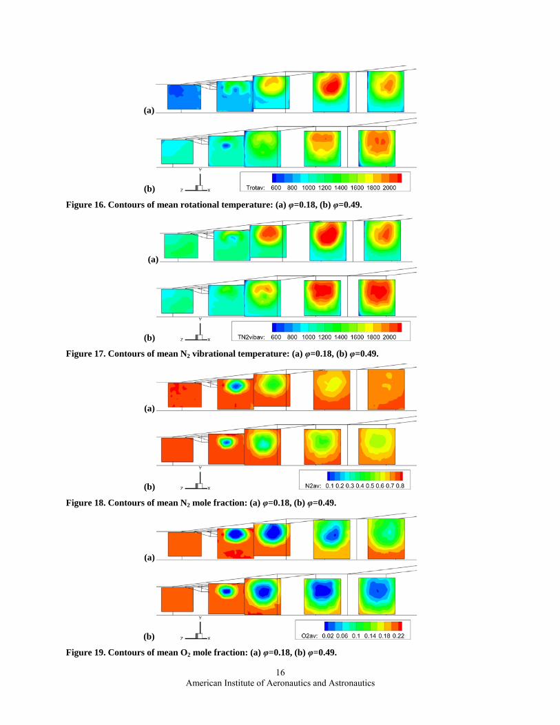
B. Parameter Distributions in the Planes Figures 15-25 show contour plots of the mean and the standard deviation of the fitted experimental temperature

and species mole fractions for both equivalence ratios. These figures show a view (looking upstream from one side) of a three dimensional representation in which the contour plots are located where the measurements were made. Also shown are lines representing the internal flow path corners and edges, and the 3-D axes. CARS measurements were interpolated from the measurement grid to a regular 50×50 grid using Kriging interpolation prior to contour plotting. The inlet isolator is on the left, the fuel injector on the top, and flow is from left to right. The mean fraction of atomic hydrogen is plotted in Figure 15, where 2 2 / 2 2 23 . This quantity takes on the value 1 in the fuel jet and 0 in the freestream, and is useful in seeing where the fuel and its products go. It is similar to the more traditional mixture mass fraction, Z, which also is 1 in the fuel jet and zero in the free stream. However, because the molecular weight of hydrogen is small, Z takes on values near zero in most of the fuel-air plume and is less useful for visualization purposes. The plots show the penetration and spreading of the fuel plume in the streamwise direction. The plume (or jet) is small at Plane 1 but nearly fills the combustor by Plane 4. The distribution of F is similar for φ=0.18 and φ=0.49, except that at 0.49 the general levels are higher, and the center of the plume is slightly further from the injection wall. At Plane 1 the jet is smaller for φ=0.49. Since the measurement grid is quite sparse and the jet is small at this plane, contours interpolated from the grid in the fuel jet must be considered inaccurate. Mean rotational temperature is shown in Figure 16 and mean N2 vibrational temperature in Figure 17. At Plane 0, the rotational temperature is higher for φ=0.49 than for φ=0.18. This is due to the shock train that propagates into the isolator, reducing the Mach number and raising the pressure and temperature at the higher equivalence ratio. On the other hand, the vibrational temperature is similar for both equivalence ratios because N2 is vibrationally frozen at conditions close to the facility air heater temperature, which is the same in both cases. There is some spatial non-uniformity of the temperatures at Plane 0, as was discussed. At the first plane after fuel injection, the temperatures

0

500

1000

1500

2000

2500

0 500 1000 1500 2000 2500

TN

2vib

Trot

Plane 0

Plane 1

Plane 2

Plane 3

Plane 4

Equilibrium

0

500

1000

1500

2000

2500

0 500 1000 1500 2000 2500

TN

2vib

Trot

Plane 0

Plane 1

Plane 2

Plane 3

Plane 4

Equilibrium


15

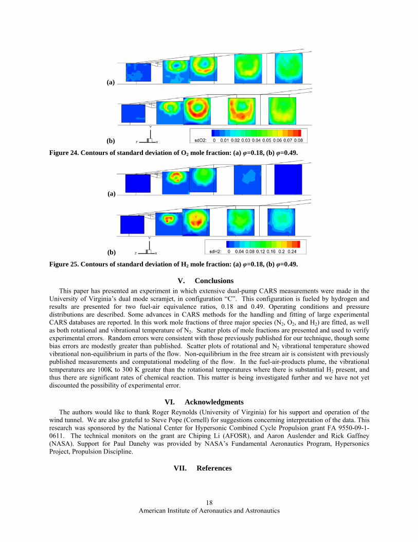
rise at the periphery of the fuel jet on the top wall side, indicating the start of combustion. At Plane 2 the region of combustion has wrapped around and engulfed the fuel plume while at Plane 3 the temperature has continued to rise and the distribution is more axially symmetric. At Plane 2 the N2 vibrational temperature in the plume is higher than the rotational (except at the edges) by 200K - 300 K, as noted earlier. For φ=0.18 the rotational and vibrational temperatures agree well with each other at Planes 3 and 4, and fall going from Plane 3 to Plane 4 due to the completion of combustion of H2 (the peak level of H2 is ~0.05 at Plane 3 and H2 is not measureable at Plane 4) and acceleration and mixing of the plume with air in the diverging duct. For φ=0.49 the vibrational temperature in the plume is higher than the rotational at Planes 3 and 4, and is still high at Plane 4 due to continuing heat release by combustion (the peak level of H2 is ~0.25 at Plane 3 and falls to ~0.10 at Plane 4). A general trend in the comparison between rotational and vibrational temperature is that the temperatures seem to be closer to equilibrium in regions of the flow where there is a significant fraction of H2 present, and thus significant rates of chemical reaction are taking place. This is consistent with what might be expected if the products of reaction were initially formed in a non-equilibrium state. But, we have not yet excluded the possibility of some type of measurement error as the cause for this difference. This matter will be investigated in the future. Mean mole fraction of N2 is shown in Figure 18, of O2 mole fraction in Figure 19, and of H2 mole fraction in Figure 20. The N2 tracks where air has mixed into the fuel plume, and shows both the growth of the plume and the penetration of air to the center. As expected, levels of N2 in the plume are generally higher for φ=0.18 than for φ=0.49. The O2 follows the N2, except that as combustion takes place in the plume it is consumed. Thus, towards the center of the plume O2 levels fall to zero. Since, as shown in Figure 20, H2 is almost completely consumed by Plane 3 for φ=0.18, O2 levels at the center of the plume have risen above zero at Plane 4. Standard deviation of rotational temperature and N2 vibrational temperature are shown in Figure 21 and in Figure 22 respectively. These standard deviations are close to zero in the freestream, generally higher at the periphery and towards the bottom side of the plume than at the center, and scale in amplitude with the peak mean temperatures. There appear to be some high fluctuations in vibrational temperature at a few points where the H2 levels are highest. These points are probably spurious due to fitting for vibrational temperature where N2 levels are low. Standard deviations of mole fraction N2 (Figure 23) and mole fraction O2 (Figure 24) are also close to zero in the freestream (as expected), and peak at the edge of the fuel plume. The absence of O2 at the center of the plume ensures that fluctuations levels there are small. Standard deviation of H2 (Figure 25) generally follows the distribution of H2 itself. The measurements described in this paper will be useful in the in the development and validation of computational models. One such effort, described by Fulton et al.,15 contains comparisons between them and computational modeling using large eddy simulation models.

(a)

(b)

Figure 15. Contours of mean atomic fraction (F): (a) φ=0.18, (b) φ=0.49. The planes from left to right are at x/H=-10.3, 6.1, 18.1, 38, and 56.1 (Planes 0, 1, 2, 3, and 4) respectively.


16

(a)

(b)

Figure 16. Contours of mean rotational temperature: (a) φ=0.18, (b) φ=0.49.

(a)

(b)

Figure 17. Contours of mean N2 vibrational temperature: (a) φ=0.18, (b) φ=0.49.

(a)

(b)

Figure 18. Contours of mean N2 mole fraction: (a) φ=0.18, (b) φ=0.49.

(a)

(b)

Figure 19. Contours of mean O2 mole fraction: (a) φ=0.18, (b) φ=0.49.


17

(a)

(b)

Figure 20. Contours of mean H2 mole fraction: (a) φ=0.18, (b) φ=0.49.

(a)

(b)

Figure 21. Contours of standard deviation of rotational temperature: (a) φ=0.18, (b) φ=0.49

(a)

(b)

Figure 22. Contours of standard deviation of N2 vibrational temperature: (a) φ=0.18, (b) φ=0.49.

(a)

(b)

Figure 23. Contours of standard deviation of N2 mole fraction: (a) φ=0.18, (b) φ=0.49.


18

(a)

(b)

Figure 24. Contours of standard deviation of O2 mole fraction: (a) φ=0.18, (b) φ=0.49.

(a)

(b)

Figure 25. Contours of standard deviation of H2 mole fraction: (a) φ=0.18, (b) φ=0.49.

V. Conclusions This paper has presented an experiment in which extensive dual-pump CARS measurements were made in the

University of Virginia’s dual mode scramjet, in configuration “C”. This configuration is fueled by hydrogen and results are presented for two fuel-air equivalence ratios, 0.18 and 0.49. Operating conditions and pressure distributions are described. Some advances in CARS methods for the handling and fitting of large experimental CARS databases are reported. In this work mole fractions of three major species (N2, O2, and H2) are fitted, as well as both rotational and vibrational temperature of N2. Scatter plots of mole fractions are presented and used to verify experimental errors. Random errors were consistent with those previously published for our technique, though some bias errors are modestly greater than published. Scatter plots of rotational and N2 vibrational temperature showed vibrational non-equilibrium in parts of the flow. Non-equilibrium in the free stream air is consistent with previously published measurements and computational modeling of the flow. In the fuel-air-products plume, the vibrational temperatures are 100K to 300 K greater than the rotational temperatures where there is substantial H2 present, and thus there are significant rates of chemical reaction. This matter is being investigated further and we have not yet discounted the possibility of experimental error.

VI. Acknowledgments The authors would like to thank Roger Reynolds (University of Virginia) for his support and operation of the

wind tunnel. We are also grateful to Steve Pope (Cornell) for suggestions concerning interpretation of the data. This research was sponsored by the National Center for Hypersonic Combined Cycle Propulsion grant FA 9550-09-1-0611. The technical monitors on the grant are Chiping Li (AFOSR), and Aaron Auslender and Rick Gaffney (NASA). Support for Paul Danehy was provided by NASA’s Fundamental Aeronautics Program, Hypersonics Project, Propulsion Discipline.

VII. References


19

1 McDaniel, J.C., Chelliah, H., Goyne, C.P., Edwards, J.R., Givi, P., Cutler, A.D., “US National Center for Hypersonic Combined Cycle Propulsion: An Overview,” AIAA-2009-7280, 16th AIAA/DLR/DGLR International Space Planes and Hypersonic Systems and Technologies Conference, Bremen, Germany, Oct 2009. 2 Lucht, R.P., “Three-laser coherent anti-Stokes Raman scattering measurements of two species,” Optics Letters, Vol. 12, No. 2, February 1987, pp. 78-80. 3 Hancock, R.D., Schauer, F.R., Lucht, R.P. and Farrow, R.L., “Dual-pump coherent anti-Stokes Raman scattering measurements of nitrogen and oxygen in a laminar jet diffusion flame,” Applied Optics, Vol. 36, No. 15, 1997. 4 Cutler, A.D., Danehy, P.M., Springer, R.R., O’Byrne, S., Capriotti, D.P., DeLoach, R., “Coherent Anti-Stokes Raman Spectroscopic Thermometry in a Supersonic Combustor,” AIAA J., Vol. 41, No. 12, Dec. 2003. 5 O’Byrne, S., Danehy, P.M., Tedder, S.A., Cutler, A.D., “Dual-Pump Coherent Anti-Stokes Raman Scattering Measurements in a Supersonic Combustor,” AIAA Journal, Vol. 45, No. 4, p. 922-933, April 2007 6 Cutler, A.D., Magnotti, G., “CARS Spectral Fitting with Multiple Resonant Species Using Sparse Libraries,” J. Raman Spectroscopy, Vol. 42, Issue 11, 2011, pp. 1949-1957. 7 Magnotti, G., Cutler, A.D., Herring, G.C., Tedder, S.A., Danehy, P.M., “Saturation and Stark Broadening Effects in Dual-Pump CARS of N2, O2 and H2,” J. Raman Spectroscopy, Vol. 43, Issue 5, May 2012, pp. 611–620. 8 Magnotti, G., Cutler, A.D., Danehy, P.M., “Development of a Dual-Pump CARS System for Measurements in a Supersonic Combusting Free Jet,” AIAA-2012-1193, 50th AIAA Aerospace Sciences Meeting, Nashville, TN, January, 2012. 9 Rockwell, R.D., Goyne, C.P., Rice, B.E., Tatman, B.J., McDaniel, J.C., and Edwards, J.R., “Close-collaborative Experimental and Computational Study of a Dual-mode Scramjet Combustor,” AIAA-2012-0113, 50th AIAA Aerospace Sciences Meeting and Exhibit, Nashville, TN, 2012. 10 Cutler, A.D., Magnotti, G., Cantu, L., Gallo, E., Danehy, P.M., Rockwell, R.D., Goyne, C.P., McDaniel, J.C., “Dual-Pump CARS Measurements in the University of Virginia's Dual-Mode Scramjet: Configuration “A”,” AIAA-2012-0114, 50th AIAA Aerospace Sciences Meeting and Exhibit, Nashville, TN, 2012. 11Fulton, J.A., Edwards, J.R., Hassan, H.A., Rockwell, R.D., Goyne, C.P., McDaniel, J.C., Smith, C., Cutler, A.D., Johansen, C., Danehy, P.M., Kouchi, T., “Large-eddy / Reynolds-averaged Navier-Stokes Simulation of a Dual-Mode Scramjet Combustor,” AIAA-2012-0115, 50th AIAA Aerospace Sciences Meeting, Nashville, TN, Jan. 2012. 12Cutler, A.D., Magnotti, G., Cantu, L.M.L., Gallo, E.C.A., Danehy, P.M., Baurle, R., Rockwell, R.D., Goyne, C.P., McDaniel, J.C., “Measurement of Vibrational Nonequilibrium in a Supersonic Freestream using Dual-Pump CARS,” AIAA Paper 2012-3199, 28th AIAA Aerodynamic Measurement Technology, Ground Testing, and Flight Testing Conference, New Orleans, 25-28 June 2012. 13 Krauss, R.H., McDaniel, J.C., Scott J.E., Whitehurst, R.B., Segal, C., Mahoney, G.T., and Childers, J.M., “Unique, clean-air, continuous-flow, high-stagnation-temperature facility for supersonic combustion research,” AIAA Paper 88-3059, July, 1988. 14 Krauss, R.H., and McDaniel, J.C., “A Clean Air Continuous Flow Propulsion Facility,” AIAA Paper 92-3912, July, 1992. 15 Fulton, J.A., Edwards, J.R., Hassan, H.A., McDaniel, J.C., Goyne, C.P., and Rockwell, R.D., “Continued RANS / Hybrid LES-RANS Simulation of a Hypersonic Dual-Mode Scramjet Combustor,” to be presented at the 51st AIAA Aerospace Sciences Meeting, Grapevine, TX, Jan. 2013. 16 Magnotti, G., Cutler, A.D., Danehy, P.M., “Beam Shaping for CARS Measurements in Turbulent Environments,” Applied Optics, Vol. 51, Issue 20, 2012, pp. 4730-4741. 17 Bivolaru, D., and Herring, G. C., “Focal Plane Imaging of Crossed Beams in Non-linearOptics Experiments,” Review of Scientific Instruments Vol. 78, No. 5, 2007. 18 Palmer, R.E, The CARSFT Computer Code for Calculating Coherent Anti-Stokes Raman Spectra: User and Programmer Information, Sandia report SAND89-8206, Feb 1989. 19 Kojima J., Nguyen Q., “Quantitative analysis of spectral interference of spontaneous Raman scattering in high-pressure fuel rich H2-air combustion,” Journal of Quantitative Spectroscopy & Radiative Heat Transfer, Vol. 94, 2005, pp 439-466, 2005. 20 Vincenti W.G., Kruger, C.H., Introduction to physical gas dynamics, John Wiley, New York, 1965.

Documents

Dual-Pump CARS Measurements in the University of Virginia ... · American Institute of Aeronautics and Astronautics 1 Dual-Pump CARS Measurements in the University of Virginia's Dual-Mode