Embed Size (px)
Citation preview

DUALISM AND MACROECONOMIC VOLATILITY
PHILIPPE AGHION
ABHIJIT BANERJEE
THOMAS PIKETTY
This paper develops a simple macroeconomic model that shows that combin-ing capital market imperfections together with unequal access to investmentopportunities across individuals can generate endogenous and permanent uctua-tions in aggregate GDP investment and interest rates Reducing inequality ofaccess may be a necessary condition for macroeconomic stabilization Moreovercountercyclical scal policies have a role to play in our model savings areunderutilized in slumps because of the limited debt capacity of potential investorsTherefore the government should issue public debt during recessions in order toabsorb those idle savings and nance investment subsidies or tax cuts forinvestors
The most important single fact about saving and investmentactivities is that in our industrial society they are generallydone by different people and for different reasons ( ) Foryears there might tend to be too little investment leading todeation losses excess capacity and unemployment Forother years there might tend to be too much investmentleading to periods of chronic inationmdashunless prudent andproper public policies in the scal and monetary elds arefollowed [Paul A Samuelson Economics 8th edition 1970pp 196ndash198]
I INTRODUCTION
The idea that the separation of savers and investors hasimplications for the short-run macroeconomic stability of aneconomy is an idea that goes back at least to Keynes [1936] andHarrod [1939] This paper represents an attempt to address thisquestion within the framework of a simple macroeconomic modelwith explicit micro-foundations
We are grateful to Pinar Bagci for research assistance to seminar partici-pants at University College London London School of Economics New YorkUniversity Harvard University Massachusetts Institute of Technology CEMFI(Madrid) the 1996 CEPR Economic Theory Symposium in Gerzensee the 1997CEPR Macro Symposium in Athens and in particular to Olivier BlanchardPatrick Bolton Ricardo Caballero Peter Diamond and the referees for helpfulsuggestions We thank the McArthur Foundation and its lsquolsquoCost of Inequalityrsquorsquo groupfor nancial support The second author also acknowledges nancial support fromthe National Science Foundation under grant number SBR-9422942
r 1999 by the President and Fellows of Harvard College and the Massachusetts Institute ofTechnologyThe Quarterly Journal of Economics November 1999
1359
In our model there are two dimensions of separation betweensavers and investors sheer physical separation manifested in thefact that savers and investors are often different people in thesense that many people who save are in no position to investdirectly in physical (as distinct from nancial) capital and a moremarket-based separation embodied in the constraints on theamounts investors can borrow from savers
We will justify the borrowing constraints by invoking theusual excuse of asymmetric information modeled here as an expost moral hazard problem By a careful choice of parameters weensure that the solution to this problem takes the extremelysimple form of a credit multiplier In other words there is aconstant n 1 such that anyone who wants to invest an amount Imust have assets of at least n I1
There are a number of reasons why not all savers are alsoinvestors in the sense of being able to invest in physical capitalFirst being able to invest may be crucially dependent on havingcertain skills ideas and connections for the vast majority ofindividuals the idea of using onersquos savings to borrow additionalfunds in order to open a new factory or purchase capital equip-ment makes no sense at all Second unequal access to investmentopportunities may just be an extreme consequence of the creditconstraints themselves many investments are indivisible andrequire a certain minimum investment In a world where capitalmarkets are imperfect this means that the investor would have toput up a minimum amount of his own wealth those who cannotafford this minimum amount will not be able to make directinvestments in production and will have to put their money in abank that then lends their savings to active investors Thirddistances may limit the ability of investors to invest the invest-ment might require the investor to live and work in the citywhereas he may have other reasons for wanting to live in a villageInvestors may also be restricted by social distance investing inmost industries involves some degree of cooperation with inves-tors in other industries and even with investors in other rms inthe same industry Therefore if an industrial sector is dominatedby people from one social group and people from this social groupare known to cooperate better with their own (perhaps for the
1 There is now a large body of evidence documenting that such borrowingconstraints have large effects on investor behavior even in countries like theUnited States which have well-developed capital markets see for exampleFazzari Hubbard and Petersen [1988] and Fazzari and Petersen [1993]
QUARTERLY JOURNAL OF ECONOMICS1360
usual repeated-games reasons) outsiders may hesitate to investin this sector Finally government regulations may restrict theability of certain social groups to invest in certain assets2
We model this physical separation of savers and investors byintroducing an asset that we call active investment (eg starting arm) which has the highest return of all assets and which is onlyaccessible to already existing businesses and their owners and toa xed fraction of the labor force We measure the separation by aconstant micro which measures the share of labor income going tothose who can actively invest (say the managerial elite)
The main contribution of the paper is the development of atractable framework for studying the business cycle implicationsof this kind of separation between savers and investors The rstresult in the paper tells us that a high degree of such separationleads the economy to uctuate around its steady-state growthpath More specically it is shown that under a condition that inour model turns out to take the very simple form of micro n implyingboth a relatively high degree of physical separation of savers andinvestors and a poorly functioning capital market the economyalways converges to a cycle around its trend growth path unless microis very small (or n very large)
The logic behind the endogenous cycles is straightforwardPeriods of slow growth are periods when savings are plentifulrelative to the limited debt capacity of potential investors whichimplies a low demand for savings and therefore low equilibriuminterest rates This in turn implies that the investors can retain ahigh proportion of their prots (since the interest rate and hencethe debt burden on investors is low) which allows them to rebuildtheir reserves and debt capacity and expand their investmentThis in turn generates more prots and more investment untileventually planned investment runs ahead of savings forcing theinterest rates to rise Now the debt burden on the investors isgoing to be higher retained earnings will be lower and invest-ment will collapse taking us back to a period of slower growth
It is worth noting that this endogenous cycle is a product oftwo distinct forces On the one hand high investment begets highprots and high investment On the other high investmentpushes up interest rates and reduces future prots and invest-ment The rst causes output to be positively serially correlated
2 For example in colonial India under the Punjab Land Tenancy act thecolonial administration in the Punjab restricted the right to own land to certainlsquolsquopeasantrsquorsquo castes
DUALISM AND MACROECONOMIC VOLATILITY 1361
the second generates a negative serial correlation Depending onwhich of these forces dominates the overall correlation of outputmay be positive or negative In particular we show that if creditconstraints are severe and the fraction of active investors is lowthen booms cannot last forever in other words the second forcewill eventually exhaust the debt capacity of investors and pushthe economy into recession
It is also worth emphasizing that cyclical uctuations in thisworld are always inefficient the economy cycles because it hasphases when savings are underutilized in the sense of beinginvested in an inferior asset In this sense our model partiallycaptures the Keynesian idea that slumps are associated with aliquidity trap3
The cycle however is just one of three possibilities if n micro sothat the degree of separation is low we have a permanent boomthe economy converges to a stable growth path where all availablesavings are always invested in the high-return activity While ifeither n is very high or micro is very low the economy converges to apermanent slump in the sense of permanently underutilizing itssaving
Of these three cases the highest trend growth rates corre-spond not surprisingly to the permanent boom case in this casethe growth rate is exactly the Harrod-Domar growth rate In bothother cases the trend growth rate is always lower than theHarrod-Domar growth rate but a priori we cannot tell which ofthe two rates is higher
These three types of economies also differ in their response toshocks where the degree of separation is low that is in what wehave called a permanent boom economy the full effect of atemporary productivity shock registers immediately in the out-put When the degree of separation is higher responses to shocksare more gradual and therefore there is more persistence inchanges in output
A permanent positive productivity shock raises the growthrate in a permanent boom economy and the new higher growthrate is achieved immediately By contrast in a permanent slumpeconomy the full impact of the shock on the growth rate comesabout only gradually The effect in the cyclical economy turns out
3 However since we do not have a notion of liquidity in our model we cannotcapture the Keynesian idea that in a liquidity trap the inferior asset that savershold is also a very liquid asset
QUARTERLY JOURNAL OF ECONOMICS1362
to be more complex than in either of the two previous casesbecause one has to take account of the effect of higher interestrates generated by the positive productivity shock on the length ofthe subsequent slump It turns out that in some cases a positiveproductivity shock can actually lower the average growth rate byprolonging the slump
The overall picture that emerges from our analysis is thateconomies with less developed nancial markets and a sharperphysical separation between savers and investors will tend to bemore volatile and to grow more slowly For a number of obviousreasons both of these dimensions of separation are likely to begreater in emerging market economies (EMEs) which in turnmay explain why macroeconomic volatility tends to be larger inthese economies than in the more developed economies4
However there is at least some evidence that this kind ofmechanism based on the functioning of the credit market is alsorelevant for understanding the business cycle properties of moredeveloped economies
For example we believe that our analysis in this paper and insubsequent work by Aghion Bacchetta and Banerjee [1998] mayshed some light on the case of advanced market economies such asFinland where nancial development (in terms of our parametern ) however is still lagging behind and which has experiencedhigh macroeconomic volatility over the past decade (see Honkapo-hja and Koskela [1998]) And even in nancially developedeconomies like the United States the mechanism we describe inthis paper may remain pertinent for the case of small investorswhose investments turn out to be signicantly correlated withcurrent cash ows (see Bernanke Gertler and Gilchrist [1998])and who therefore constitute a less nancially developed enclavewith the U S economy The case for a credit channel in thetransmission of shocks to the U S economy has been argued for invarious contributions going back at least to the work of Haberler
4 Some reasons why the extent of separation of savers and investors may beespecially large in EMEs include poor transportation facilities which exaggeratephysical distances and limit certain types of investment to those who live closeenough to the natural locale for the investment badly dened and poorly enforcedproperty rights make loan transactions harder social segmentation on the basis ofcaste and tribe often acts to limit entry into specic industries and high levels ofsocial and economic inequality might mean that only a small fraction of thepopulation has the wherewithal to be investors
DUALISM AND MACROECONOMIC VOLATILITY 1363
[1964]5 and more recently in a number of papers by Bernanke andGertler6
Given the inefficiency of cyclical uctuations in our modelthere is clearly a potential role for countercyclical macro policiesSince slumps are times where there are some idle savings that arenot being used efficiently because of the limited debt capacity ofpotential investors a natural strategy for recovery is to issuepublic debt in recessions in order to absorb those idle savings andnance investment subsidies or tax cuts for businesses We showthat under some conditions such policies can at the same timerestore maximum growth and raise the saversrsquo welfare
Of course a different policy perspective on our model wouldbe to argue that it stresses the importance of structural reformsthat aim at reducing the extent of separation of savers andinvestors This is especially likely to be important in situationswhere the appropriate countercyclical policies are difficult tocarry out (for example because the extent of separation ischanging rapidly over time and in situations where countercycli-cal policies have adverse distributional consequencesmdashthe poli-cies suggested by our model always help investors but sometimesat the cost of savers) Structural reforms may in such cases be anecessary condition for the success of stabilization policies
Our model is far from being the rst that emphasizes the roleof the separation between savers and investors as a source ofmacroeconomic volatility This general point can be found in theworks of Keynes [1936] Harrod [1939] among others but in theirmodels the primary source of instability is the exogenous instabil-ity in the investment rate
Goodwinrsquos [1967] model of growth cycles is closer to ours inthat it also describes cycles as the outcome of a dynamic processwith the imbalance between investors and savers changing endoge-nously over time although Goodwinrsquos mechanism operates throughthe equilibrium wage rate rather than the equilibrium interestrate (for some evidence that our mechanism is important inpractice see subsection III4) Despite this difference the twostories are entirely consistent with each other and share thecommon prediction that downturns in economic activity are
5 Who in turn refers to Hawtrey and Wicksell6 These authors have a number of papers of which perhaps the most
immediately relevant is their recent survey of the literature [Bernanke andGertler 1995a 1995b)
QUARTERLY JOURNAL OF ECONOMICS1364
caused by the decline of investorsrsquo investment capacity Where thepapers differ most is in the modeling style Unlike ours Goodwinrsquosmodel has no explicit micro-foundations and therefore does notallow for rigorous policy analysis and checks of robustness InAppendix 2 we show how our model can easily be extended inorder to offer a micro-founded version of a Goodwin cycle
Our paper and all papers on the role of debt in the transmis-sion of business cycles owe a lot to the seminal paper by Bernankeand Gertler [1995a] which in turn was inuenced by the mucholder ideas of Fisher [1933] and his followers on debt deation Asin Bernanke and Gertler the presence of debt and borrowing inour model makes the effects of productivity and other shocks morepersistent than they would otherwise be and also induces amultiplier with respect to these shocks Where we go beyondBernanke and Gertler is in emphasizing the general equilibriumeffects of such shocks a shock that increases prots now willincrease debt capacity and therefore investment in the future butit will also raise interest rates and the debt burden whichdiscourages investment Therefore in the medium run invest-ment might go down rather than up as a result of the increase inprots It is this general equilibrium mechanism that allows ourmodel unlike that of Bernanke and Gertler to have oscillationsand endogenous cycles
General equilibrium effects also play a role in the paper byKiyotaki and Moore [1997] on the business cycle effects ofborrowing constraints In their paper a shock to prots raisesinvestment which in turn increases the price of collateral whichmakes the investors (who already own collateral) richer andinduces more investment Of course this process is accompaniedby an increase in the debt burden but the increase in the debtburden is matched by the increase in prots coming from the extrainvestment that caused the debt to go up in the rst place unlikein our model there is no interest rate effect that would cause thedebt burden to go up disproportionately Consequently in theirbasic model the credit market effects only amplify and draw outthe initial shock there is no endogenous counteracting effect ofthe kind that we emphasize and that give us the endogenousoscillations Such a counteracting effect which causes the economyto have persistent oscillations in response to a shock does appearin a generalized version of their model but in order to have it theyneed to introduce lags in the response of investment to changes in
DUALISM AND MACROECONOMIC VOLATILITY 1365
borrowing capacity While such lags may well be plausible it is notclear to what extent it is the lags rather than the basic mecha-nisms of the model that are driving the cycles7 Moreover theyonly report damped oscillations and do not provide us withconditions under which the model will converge to a limit cycle
Finally our focus on the interplay between credit imperfec-tions and the dynamics of distribution relates this work to theliterature on inequality credit-market imperfections and growth(see eg Banerjee and Newman [1993] Galor and Zeira [1993]Aghion and Bolton [1997] and Piketty [1997]) However theemphasis on short-run uctuations directs our attention toward avery different kind of inequality than the one emphasized in thisliterature We nd that from the point of view of short-runstability it is the inequality between savers and investors ratherthan the inequality between the rich and the very poor (whoneither invest nor save very much) that matters
The paper is organized as follows Section II outlines the basicframework In Section III the basic model is analyzed and thebasic results about stability and the nature of the response toshocks are derived Section IV discusses the impact of governmentpolicies on volatility and average growth
II BASIC FRAMEWORK
The economy has one nonproduced input (labor) and oneproduced good which serves both as a capital input and as aconsumption good Each agent is endowed with one unit of laborat each period
Technology The production function for the one producedgood is F(KL) 5 AK b L12 b 5 Y In order to focus our attention uponthe capital market equilibrium we assume that the labor markettakes a very simple form the wage rate is permanently equal to
7 Freixas and Rochet [1997] have a discussion of the Kiyotaki-Moore paperwhere they claim that it can be adapted to have oscillations even without the lagsby adding an alternative use for the collaterizable asset In their version of themodel as the amount of borrowing grows and more and more of the collaterizableasset gets used in the production sector less and less of it goes to the alternativeuse This reduces prots because the alternative use is actually more protablethan production However this seems to rely on the investors not optimizingotherwise they would always put the asset to its most protable use rather thanuse it for increasing production
QUARTERLY JOURNAL OF ECONOMICS1366
one and rms can always hire as much labor as they wish to atthat price8 In equilibrium
shy F
shy L5 1 THORN L 5 ((1 2 b )A)1 b K
THORN Y 5 s K
with s 5 A((1 2 b )A)(12 b ) b )
This is an example of what has been called an AK model andtherefore will generate positive long-run growth Also note thatthe labor and capital shares of nal output are given by the usualformulas (shy Y shy L)L 5 (1 2 b ) s K and ( shy Y shy K)K 5 b s K9
Investment Possibilities Not everyone has direct access toinvestments in production Those who cannot invest directly inproduction (the lsquolsquononinvestorsrsquorsquo or the lsquolsquolendersrsquorsquo or lsquolsquosaversrsquorsquo) caneither lend at the current interest rate r to those who can invest inproduction (the lsquolsquoinvestorsrsquorsquo or the lsquolsquoborrowersrsquorsquo) or invest in alow-yield asset that yields a return s 2 with s 2 s 1 5 b s 10 We willthink of this asset as storage but it could as well be some otherproduction technology (or some government bond see Section IVbelow) In addition to rmsrsquo owners the investorsrsquo class alsoincludes a xed fraction of the labor force (say the managers whohave sufficient knowledge about direct investment opportunities)and the size of this group is measured by its share micro in total laborincome The case micro 5 0 is the case where all productive invest-ment is carried out directly by businesses and their owners andthe lsquolsquohousehold sectorrsquorsquo can only lend its savings to the lsquolsquobusinesssectorrsquorsquo (or invest in the low-yield asset) At the other extreme thecase micro 5 1 is the case where everyone can directly invest his own
8 Therefore we are implicitly assuming that the size of the labor force growsat least as fast as the capital stock such that the wage rate is xed to one forstandard labor supply reasons (agents are prepared to sell their labor unit at anyprice higher than or equal to one)
9 Instead of assuming an unlimited labor supply at price 1 one could alsoassume a xed labor supply L0 and introduce an aggregate capital accumulationexternality a la Frankel [1962] or Romer [1986] in order to obtain an AK modelwith steady-state long-run growth if Y 5 AK b L1 2 b Ka
g where Ka is the aggregatecapital stock (the effects of which are not internalized by individual rms) then ifg 5 1 2 b and L L0 we have Y 5 s K with s 5 AL0
1 2 b and the capital share(respectively the labor share) of output is again equal to b Y (respectively(1 2 b )Y ) These alternative assumptions would leave our analysis of macroeco-nomic volatility unaffected while extending it beyond the Harrod-Domar case tothe case of more standard AK technologies
10 We assume the nancial intermediation process between lenders andinvestors to be perfectly competitive so that lenders always get the full return totheir savings This allows us to avoid dealing with the banking sector in whatfollows
DUALISM AND MACROECONOMIC VOLATILITY 1367
savings into the high-yield production activity and where there isthus no separation between savers and investors
Capital Market Imperfection Due to standard incentive-compatibility considerations an investor with initial wealth Wcan invest at most W n where 1 n 1 is a credit multiplier11
Credit constraints vanish as v tends toward 0 while v 5 1 is thepolar case where the credit market collapses and investors canonly invest their own wealth
Determination of the Interest Rate The interest rate is theone price in this model that is determined endogenously Thelinearity of the production technology implies that the equilib-rium interest rate will be exactly equal to the rate of return s 1 5b s whenever planned investment in production is higher thanaggregate savings and it will drop down to s 2 in the opposite case(see below)12 Our results can be extended to a more general modelwhere the interest rate changes smoothly over time (see subsec-tion III4 below)
The Timing of Events The timing of events within in eachperiod t is depicted in Figure I
Borrowing and lending take place at the beginning of theperiod (which we denote by t 2 ) at an interest rate that is
11 An explicit microeconomic derivation of this (constant) credit multiplier isdeveloped in Appendix 1 where we also discuss the robustness of our analysis toalternative microeconomic foundations whereby the multiplier n ends up depend-ing upon the interest rate r See also our discussion in subsection III4 below
12 Throughout the paper we will adopt the convention that interest rates aswell as the growth rates refer to the gross rate (ie one plus the net rate)
FIGURE IThe Timing
QUARTERLY JOURNAL OF ECONOMICS1368
determined as indicated above by the comparison between plannedinvestments and savings at t 2
Everything else occurs at the end of the period (which wedenote by t 1 ) rst the returns to investments are realizedsecond the repayment of debt from borrowers to lenders thirdthe consumption decisions and the savings decisions that in turnwill determine the total amount of available savings at thebeginning of next period (ie at (t 1 1) 2 )
Savings Behavior For simplicity we assume a linear savingbehavior all agents save a xed fraction (1 2 a ) of their totalend-of-period wealth and consume a xed fraction a (see subsec-tion III4 below for a discussion of alternative assumptions)
Now that the model has been fully laid out we can analyzethe dynamics of the underlying economy and in particular try tounderstand why the inequality in investment opportunities be-tween investors and noninvestors in other words the separationbetween savings and investments can generate macroeconomicvolatility
III THE MECHANICS OF THE MODEL
III1 The Basic Dynamic Relationships
Let W Bt and WL
t denote the wealth of investors (borrowers)and noninvestors (lenders) at the beginning of period (t 1 1) Totalsavings from previous period t are by denition equal to
St 5 W Bt 1 W L
t
Total planned investments in the high-yield activity at thebeginning of period (t 1 1) are equal to
I t 1 1d 5 WB
t n
Note the following1 The interest rate rt1 1 in period (t 1 1) is equal to b s 5 s 1 if
I t 1 1d St (that is whenever the investment capacity
of investors is higher than aggregate savings) and to s 2 ifI t 1 1
d St (that is whenever the investment capacity ofinvestors is lower than aggregate savings)
2 Actual investment in the high-yield activity at date (t 1 1)is equal to min (StI t1 1
d ) whereas investment in the low-yield activity (with return s 2) is equal to St 2 min (StI t 1 1
d )
DUALISM AND MACROECONOMIC VOLATILITY 1369
3 Current borrowing by investors is equal to the differencebetween actual investment in the high-yield activity andtheir initial wealth W B
t During periods when investment demand is higher than
aggregate savings all savings are invested in the high-yieldactivity (with total return s ) and the growth rate of the economytakes its maximum value g 5 (1 2 a ) s 13 We will call theseperiods lsquolsquoboomsrsquorsquo Conversely during periods when investmentdemand is less than aggregate savings a positive fraction ofaggregate savings is invested in the low-yield activity so that thegrowth rate is smaller than g We will call these periodslsquolsquoslumpsrsquorsquo We can now obtain the following equations describingthe dynamic evolution of capital accumulation between twoconsecutive periods During a boom (ie if I t 1 1
d St)
(B) WBt 1 1 5 (1 2 a )[micro(1 2 b ) s (WB
t 1 W Lt )
1 b s (W Bt 1 W L
t ) 2 b s W Lt ]
W Lt1 1 5 (1 2 a )[(1 2 micro)(1 2 b ) s (WB
t 1 W Lt ) 1 b s WL
t ]
In other words given that all available savings (W Bt 1 W L
t )are invested in the high-yield activity during a boom totalrevenue from this activity is equal to s (W B
t 1 W Lt ) A fraction
(1 2 b ) of that revenue remunerates the labor force with inves-tors (respectively noninvestors) representing a fraction micro (respec-tively 1 2 micro) of the total labor share of output Second whileborrowers realize the yield rate of return b s on capital investment(W B
t 1 W Lt ) they must repay the high interest rate r 5 b s on the
amount W Lt they have borrowed from the lenders (hence the term
2 b s W Lt in the right-hand side of the rst equation which
corresponds to the term b s W Lt in the right-hand side of the second
equation)Similarly during a slump (ie if I t1 1
d St)
(S) W Bt1 1 5 (1 2 a ) micro(1 2 b ) s middot
1
nWB
t 1 b s1
nW B
t 2 s 2
1
n2 1 W B
t
W Lt1 1 5 (1 2 a ) (1 2 micro)(1 2 b ) s middot
1
nW B
t 1 s 2WLt
Namely given that only the amount WBt n can be invested in
13 g is the standard Harrod-Domar growth rate ie the product of thesavings rate by the outputcapital ratio
QUARTERLY JOURNAL OF ECONOMICS1370
the high-yield activity during a slump this activity will generate arevenue equal to s W B
t n A fraction (1 2 b ) of that revenueremunerates labor with borrowers (respectively lenders) gettinga fraction micro (respectively 1 2 micro) of that revenue The fraction b ofthat revenue remunerates capital investment and thus accruesentirely to the borrowers However borrowers must pay theinterest rate s 2 on the amount (W B
t n 2 W Bt ) they borrow from the
middle-class lenders On the other hand lenders realize the rateof return s 2 on their wealth W L
t both by lending a fraction of it towealthy borrowers and by investing the complementary fractionin the low-yield activity14
Letting q t 5 St I t1 1d denote the ratio of savings over planned
investments in the high-yield activity at the beginning of period(t 1 1) simple manipulation of the above equations leads to
(B8)1
q t1 15
micro(1 2 b )
n1 b middot
1
qt
when qt 1 (ie when the economy is in a boom at the beginningof period t 1 1) and
(S8) qt1 1 51
micro(1 2 b )(s n ) 1 (1 n )b s 2 ((1 n ) 2 1)s 2[(s 2 s 2) 1 s 2qt]
when qt 1 (ie when the economy is currently experiencing aslump)
Equations (B8) and (S8) dene a simple rst-order differenceequation which allows a complete characterization of the globaldynamics of the economy
III2 Slumps and Booms
Note rst that both curves (B8) and (S8) are monotonicallyincreasing and intersect the 45deg degree line only once (fromabove) Note also that the (B8)-curve always lies above the(S8)-curve at qt 5 1 q t1 1(q t 5 1rt1 1 5 s 1) qt 1 1(qt 5 1rt 1 1 5 s 2)15
14 They lend the amount (W Bt n 2 W B
t ) to the high-yield investors and investthe remaining amount W L
t 2 (W Bt n 2 W B
t ) in the low-yield activity15 The intuition for this is quite straightforward borrowers benet from
lower interest rates at the expense of lenders Therefore the savingsinvestmentdemand ratio is lower next period if the current interest rate rt 1 1 is lower for agiven allocation of funds (if q t 5 1 all savings are invested in the high-yieldactivity irrespective of whether rt 1 1 5 s 1 or s 2) More formally when qt 5 1
qt 1 1(qt 5 1rt1 1 5 s 2) 51
(micro(1 2 b ) n ) 1 ( b n ) 2 ((1 n ) 2 1)(s 2 s )
DUALISM AND MACROECONOMIC VOLATILITY 1371
Therefore there are only three possible cases corresponding to thethree possible rankings between 1 s and b where s and b are theintersections of the (S8) and (B8) curves with the 45deg line Theseare depicted in Figures II III and IV
Figure II corresponds to the case where 1 b( s) In thiscase as is evident from the gure the economy converges to apermanent boom with qt b The long-run growth rate for theeconomy is just the Harrod-Domar growth rate g 5 (1 2 a ) s Simple manipulation of equation (B8) yields
b 5 n micro
The condition b 1 is therefore equivalent to n micro Thisnecessary and sufficient condition is very intuitive a permanentboom will occur when the fraction of the labor force that has directaccess to investments in production is sufficiently large to compen-sate for the borrowing constraints faced by these investors Thiscondition ensures that in the long run the debt capacity ofinvestors will always be sufficient for all available savings to beabsorbed and invested in the high-yield activity In particular theHarrod-Domar permanent boom regime will occur if credit con-straints are negligible ( n close to 0) or if all agents have directaccess to productive investments (micro close to 1) Converselypermanent booms will never occur if micro 5 0 ie if business protsare the only investible funds This is because if micro 5 0 then theinvestment capacity of the economy grows at rate (1 2 a )b s whilesavings grow at the higher rate (1 2 a ) s the latter will thereforealways be in excess supply after some nite time16 The conditionmicro n also shows that both dimensions of separation betweeninvestors and savers (ie n 0 and micro 1) are necessary in orderto generate slumps in the long run
Figure III corresponds to the case where 1 s( b) Here theeconomy always converges to a permanent slump (with q t s)and with a rate of growth that is less than the Harrod-Domar
qt 1 1(q t 5 1rt1 1 5 s 1) 51
(micro(1 2 b ) n ) 1 b
( s 1 5 b s s 2 implies that b ( b n ) 2 (1 n ) 2 1)(s 2 s ))16 If micro 0 then the investment capacity of the economy grows at rate
(1 2 a ) (micro(1 2 b ) s )v) 1 b s ) which is smaller than the savings growth rate iffmicro n
QUARTERLY JOURNAL OF ECONOMICS1372
growth rate (1 2 a ) s Simple manipulation of equation (S8) yields
s 5( s 2 s 2) n
micro(1 2 b ) s 1 b s 2 s 2
The necessary and sufficient condition dening the perma-nent slump regime is then given by
s 1 or equivalently micro(1 2 b ) 1 b n 1s 2
s(1 2 n )
This condition is also very intuitive permanent slumps willtend to occur when the credit multiplier is small ( n high) and fewpeople have direct access to investments in production (micro small)Note also that permanent slumps are more likely to occur if s 2 s ishigh a high s 2 s ratio implies high debt repaymentprot ratiosfor investors and therefore makes it less likely that their debtcapacity will ever be able to absorb all available savings (the samereasoning applies if the capital share b is low) The expression for
FIGURE IIThe Permanent Boom Regime
DUALISM AND MACROECONOMIC VOLATILITY 1373
s can also be used to compute the exact growth rate gs associatedwith the permanent slump regime in steady state a fraction 1s ofaggregate savings is invested in the high-yield activity (withreturn s ) while the remaining fraction 1 2 1s is invested in thelow-yield activity (with return s 2) so that the steady-state growthrate gs is given by
gs 5 (1 2 a )1
ss 1 1 2
1
ss 2 ( (1 2 a ) s )
5 (1 2 a ) s 2 1micro(1 2 b ) s 1 b s 2 s 2
n
This is always lower than the Harrod-Domar growth rateFigure IV corresponds to the case where s 1 b In this case
the gure shows that the economy keeps moving back and forthbetween booms and slumps and will eventually converge to alimit-cycle The two conditions for this case are b 1 (1 2 b )micro n 1
FIGURE IIIThe Permanent Slump Regime
QUARTERLY JOURNAL OF ECONOMICS1374
( s 2 s )(1 2 n ) and micro n These two conditions imply that aneconomy with a very high degree of separation between saversand investors as well as an economy where both groups areextremely well integrated will not cycle in the rst case there willbe a permanent slump and in the second a permanent boom17 It isonly in the intermediate case where the separation is large but nottoo large that we observe short-run instability Note that short-run instability is associated with the economy performing belowits potential (as measured by growth rates) since slumps arephases where some of the capital is put to less than optimal usethe growth rate is equal to the Harrod-Domar growth rate duringbooms (when qt 1) but is strictly below the Harrod-Domargrowth rate during recessions (when qt 1)
17 In particular a highly underdeveloped economy where businesses relyentirely on their own retained earnings to invest will not cycle
FIGURE IVThe Cycles Regime
DUALISM AND MACROECONOMIC VOLATILITY 1375
Note also that the limit cycle need not be a two-cycle asdepicted in Figure IV Figures V and VI depict n 2-cycles witheither a debt-buildup phase during which borrowers are gettingpoor relative to creditors (Figure V)18 or a prot-reconstitutionphase during which borrowers are getting richer relative tocreditorsmdashboth because creditors get the low rate s 2 on theirsavings and because borrowings are low during slumps (FigureVI)19 The relative length of boom (ie debt buildup) and slump(ie prot reconstitution) phases will depend upon the basicparameters of the model expansionary phases with debt buildupwill last longer when the slope of the (B8) curve at the point b isclose to 1 (or equivalently when b is close to 1) on the other hand
18 This case is more likely to arise when the slope of the (B8)-curve issufficiently close to 1 at b that is when b is close to 1
19 This case is more likely to arise when the slope of the (S8)-curve issufficiently close to 1 ie when
(1 n )[ s 2 2 (micro(1 2 b ) 1 b )]
is sufficiently small
FIGURE VProlonged Boom (Debt Buildup)
QUARTERLY JOURNAL OF ECONOMICS1376
the length of recession phases will go up when the slope of the(S8)-curve gets closer to 1 (in particular when n or s 2 is large as inFigure VI)
Intuitively during an expansionary phase investment (andtherefore borrowings) will go up since output and prots andtherefore the borrowing capacity of investors are growing Andthe higher the share of capital b in the revenue from thehigh-yield activity the more will prots increase over time andtherefore the longer will the investorsrsquo borrowing capacity keep onabsorbing total savings Hence the higher b the longer the debtbuildup phases On the other hand the larger s 2 or n the largerthe ratio of savings over planned investment when the economyenters a recession this together with the fact that investors mustrepay a higher interest rate s 2 to their lenders throughout therecession implies that it will take longer before the borrowingcapacity of investors can again absorb the totality of savings (atwhich point the economy can reenter a boom)
FIGURE VIProlonged Recession (Prot Reconstitution)
DUALISM AND MACROECONOMIC VOLATILITY 1377
III3 The Effects of Shocks
How does such an economy react to shocks In order toanswer this question we rst look at how the shocks move the twocurves (B8) and (S8) We will focus on two kinds of shocks shocks tos which are naturally interpreted as productivity shocks andshocks to s 2 which may be thought of either as productivityshocks (for example if this asset is thought of as home production)or as policy shocks (for example if this asset is thought of asmoney the shock could be a change in the variance of the inationrate)
It is easy to see from equation B8 that the curve (B8) isunaffected by changes in s and s 2 This should be intuitive anincrease in s during a boom increases both the return to invest-ment and the return on savings exactly in the same proportionand therefore does not affect the distribution of wealth betweenthe savers and investors (measured by q) A change in s 2 has noeffect because in a boom no one puts his money in the inferiorasset
A trivial calculation establishes that in the range in which the(S8) curve is relevant (ie as long as q 1) an increase in s and afall in s 2 lowers the (S8) curve This too should be intuitive in aslump an increase in s benets the investors but not the saverswhile a fall in s 2 hurts the savers while beneting the investors
It follows that if the economy is in a permanent boom neithera temporary nor a permanent shock to productivity (ie s goingup) has any effect on the distribution of wealth between saversand investors It does of course have an effect on the rate ofgrowth in periods where s is higher the growth rate will beproportionally higher However because there is no effect on q theentire effect on the growth rate is registered in the period of theshock In other words if the shock is permanent the economyimmediately goes to its steady-state growth rate and if it istemporary after the shock the economy grows at the same rate asbefore the shock albeit starting at a higher level of GNP Changesin s 2 have no effect for obvious reasons Figure VIIa (respectivelyVIIb) describes the dynamic effects of a permanent (respectivelytemporary) increase in s on the growth rate when the economyismdashand remainsmdashin a permanent boom20
The picture in a permanent slump economy is quite different
20 In this and the following gures we assume for simplicity that theeconomy is initially at a steady state
QUARTERLY JOURNAL OF ECONOMICS1378
FIGURE VIIaEffect of a Permanent Increase in s on a Booming Economy
FIGURE VIIbEffect of a Temporary Increase in s on a Booming Economy
Note rst that the steady-state growth rate gs is an increasingfunction of s but a decreasing function of s 2 that is the positiveeffect of a higher s 2 on the returns to the fraction of savings thatare not invested in the high-yield activity is more than offset bythe negative effect of a higher s 2 on debt repayments andtherefore on the steady-state debt capacity of investors Taxing s 2
and throwing the tax revenues away would actually increase thelong-run growth rate21
The process of convergence to the new steady state is alsoquite different from that in a permanent boom economy As can beseen from Figure VIIIa a permanent rise in s or a permanent fallin s 2 shifts the (S8) curve downward As a result q falls initiallyand then continues to fall as it converges toward its steady-statelevel Since ceteris paribus a fall in q raises the growth rate22 byshifting the distribution of wealth toward the investors the initialrise in s or fall in s 2 will end up having both a direct and indirectpositive effect on the growth rate as shown in Figure VIIIb
Similarly Figures IXa and IXb show that the growth-enhancing effects of a one-period increase in s or a one-period fallin s 2 will also persist beyond the period of the shock Moreoverthere is the possibility of a multiplier the output effect of a shockmay be larger after the shock itself has died out and the economyhas gone back to its original parameters23 This is again due to thefact that the shock shifts the distribution of wealth in favor the
21 Alternatively the government could impose interest rate ceilings so as topush the interest rate below s 2 (see Section IV below)
22 The growth rate in a slump period is given by (1 2 a )(( s q) 1 (1 2(1q) s 2)
23 Let Y0 denote the average output of the economy before the shock Y1denote the average output in the period when the shock hits and Y2 denote theaverage output in the following period right after the productivity parameter s hascome back to its initial value Assume that the economy is initially in a permanentslump For a sufficiently small initial increase in productivity from s to s 1 ds onecan show that
Y2
Y15
1
q1s 1 1 2
1
q1s 2
Y1
Y05
1
q0( s 1 ds ) 1 1 2
1
q0s 2 1
where q0 and q1 are the values of q before and right after the shock ie
q0 5 g ( s ) middot [ s 2 s 2 1 s 2q0] 5 sand
q1 5 g ( s 1 ds )[ s 1 ds 2 s 2 1 s 2q0]
where g ( s ) is the rst term in the expression for q t 1 1 in equation (S8) above
QUARTERLY JOURNAL OF ECONOMICS1380
FIGURE VIIIa
FIGURE VIIIbFIGURE VIII Effect of a Permanent Increase in s on Economy in Slump
FIGURE IXa
FIGURE IXbFIGURE IX Effect of a Temporary Increase in s on Economy in Slump
gs(t) responds nonmonotonically to temporary increase in s but it remainspermanently above the preshock steady-state level
QUARTERLY JOURNAL OF ECONOMICS1382
investors (ie shifts q down) and this distributional effect onlydies away gradually
The effects of shocks in a cyclical economy are for obviousreasons more complex In particular an increase in s has anambiguous effect on average growth in this case on the one handit increases growth during booms but on the other hand investorsend up accumulating a higher debt burden during booms whichcauses recessions to be more severe (ie with higher q ratios inrecessions) The overall effect on average growth is unclear ingeneral However for the same reasons as in the permanentslump regime an increase in s 2 will have an unambiguouslynegative effect on average growth a higher s 2 leads to higher debtrepayments during slumps and therefore both to lower growthduring and also to longer periods of slumps
The process of convergence to the new cycle after a permanentshock is potentially quite complicated (as the reader can readilyverify by moving the (S8) curve in Figures IV V or VI) and dees astraightforward classication However what remains unambigu-ously true is that unlike in the permanent boom case the growthrate will only gradually adjust to its new steady-state level
The above analysis ruled out the possibility that the shockresults in shifting the economy from one of our regimes to anotherAs is evident from the condition for the cycling case b 1 (1 2b )micro n 1 ( s 2 s )(1 2 n ) high values of s and low values of s 2 tendto move the economy away from a permanent slump toward acycle This is not necessarily a good thing it turns out that anincrease in s can actually reduce average growth by forcing theeconomy to shift from a permanent slump regime to a cyclicalregime because at least over some open parameter interval it isbetter never to have a boom than to have it some of the time24
III4 Robustness of our Results
Our results are derived in an exceedingly pared-down modeland it is legitimate to wonder whether these results would survive
24 Namely assume that micro n and consider s 5 s such that micro(1 2 b ) 1 b 5n 1 ( s 2 s )(1 2 n ) If s s the economy is in a permanent slump regime As ss the permanent slump growth rate increases gs g 5 (1 2 a ) s But if s goesabove s then the economy exits the permanent slump regime and begins to cyclethat is the average growth rate falls below its Harrod-Domar value It follows thatat least over some range [ s s 1 e ] the average growth rate is a decreasingfunction of s (although there need not exist any discontinuity in average growthrates) For the same reasons the average growth rate is an increasing function ofs 2 at least over some range [ s 2 2 e s 2] in the region where an increase in s 2 shiftsthe economy from a cyclical regime to a permanent slump
DUALISM AND MACROECONOMIC VOLATILITY 1383
in a more realistic model Here we make a number of commentsemphasizing the directions in which the model can be extendedwithout losing our basic results
1 In the present version of the model the equilibriuminterest rate r uctuates discontinuously between one high valueand one low value In a previous version of the paper weconstructed a version of the model where investors can chooseamong a continuum of technologies and therefore where theequilibrium interest rate can take on a continuum of values andshowed that we still get cycles
2 If consumption-savings decisions were taken at the begin-ning of the period instead of at the end an expected fall in interestrates would reduce savings limiting the fall in interest rates andthereby limiting the extent of uctuation However if this were toeliminate all uctuations the interest elasticity of savings wouldhave to be quite high which it does not seem to be [Attanasio andWeber 1993] The same comment applies to whether our resultwill change if savers are forward-looking
3 Throughout our analysis in this paper we have assumedthat individuals with investment opportunities have the samepropensity to consume as those with no investment opportunitiesIntroducing different savings rates (1 2 a L) and (1 2 a B) forlenders and borrowers would slightly complicate the analysis ofthe model but the essential conclusions would be unchangedMoreover using the fact that the slopes of the (B8) and (S8) curvesare increasing functions of the ratio (1 2 a L)(1 2 a B) one canshow25 (i) if 1 2 a B 1 2 a L then the economy converges to apermanent slump as borrowersrsquo investment can never absorb thetotal amount of lendersrsquo savings (ii) if 1 2 a L 1 2 a B then theeconomy converges to a permanent boom as borrowersrsquo invest-ment capacity tends always to be greater than aggregate savings(WB g WB 1 WL)) (iii) in the intermediate case where (1 2 a L)and (1 2 a B) are of comparable magnitudes the economy willconverge to a limit cycle for suitable values of the parameters Inthis case we can analyze how the characteristics of the limit cycleare affected by the relative savings rates of lenders and borrowersIntuitively if 1 2 a B is relatively small compared with 1 2 a L thenbooms should be of short duration and slumps should be long-lasting as it should take a while before borrowers can reconstitutetheir investment capacity following a credit crunch Conversely if
25 The reader can verify this by looking back at Figures V and VI
QUARTERLY JOURNAL OF ECONOMICS1384
1 2 a L is small relative to 1 2 a B then booms will be long-lastingand slumps will be short
4 Even if investors were long-lived instead of living for justone period in our model they never have a reason to postponeinvestment since investment always earns a higher return thanthe cost of capital (r s 1) That is while slumps are indeed thebest period to invest (interest rates are low) investors have noreason to delay their investment until the next slump becausethey will always have more money to invest next period if theyinvest today26
5 Our results clearly depend on the interest rate beingendogenous and not given from outside as it might be forexample in a small open economy However this seems a reason-able approximation to the reality in many economies (see Feld-stein and Horioka [1980] for evidence showing that capital tendsnot to move across borders) Furthermore as we show in AghionBacchetta and Banerjee [1998] while opening a small economywith credit-constrained investors to foreign borrowing and lend-ing has the obvious effect of stabilizing interest rate movementsit may still destabilize the economy by exacerbating movements inthe real exchange rate27
6 Throughout our analysis we have taken the credit-multiplier 1 n to be independent of the level of interest rates InAppendix 1 we provide an explicit microeconomic derivation ofthis constant credit-multiplier based on ex post moral hazard onthe part of the borrower combined with an appropriate choice ofthe lendersrsquo monitoring technology It is also possible to derive acredit multiplier from an ex ante moral hazard story a la
26 On the other hand forward-looking rms may tend to accumulate savingsat a higher rate during booms (eg by cutting dividends) in order to expand theirinvestment in slumps This would also tend to reduce the amplitude of theuctuations but it should not eliminate all uctuations unless the shareholders ofthe rm are extremely patient
27 The underlying mechanism is similar to the one described in this paperexcept that the pecuniary externality which serves as the transmission variablefor generating uctuations is the real exchange rate dened as the price ofnontradable goods in terms of the tradable good More specically the basicmechanism in Aghion Banerjee and Bacchetta [1998] can be described as followssuppose that high-yield investments in the domestic economy require the use ofnontradable goods (such as real estate) as inputs to produce tradable goods Thenduring a boom the domestic demand for nontradable goods keeps going up ashigh-yield investments build up and thus so does the price of nontradablesrelative to that of tradables This together with the accumulation of debt that stillgoes on during booms will eventually squeeze investorsrsquo borrowing capacity andtherefore the demand for nontradable goods At this point the economy experi-ences a slump in which the price of nontradable goods collapses and lendablefunds ow out of the country
DUALISM AND MACROECONOMIC VOLATILITY 1385
Holmstrom and Tirole [1997] but this would give us a v(r) whichincreases with the interest rate r This in turn would tend todampen investors debt buildup during booms and thereby reducethe magnitude of subsequent slumps However one can show thatthe occurrence of cyclical (or volatile) growth patterns is stillpreserved in this case so long as n (r) does not increase too rapidlywith r28
7 We show in Appendix 1 that our results are also robust toallowing investors and savers to write long-term debt contractsIntuitively a long-term contract may allow borrowers to postponea part of the repayment on their debt to periods when they expectto be relatively cash rich and thereby limit the variation in qt Weshow in Appendix 1 that while this intuition is correct theeconomy will continue to have cycles under conditions that aresomewhat stronger than those assumed in our basic model29
8 Two empirical predictions that emerge from our analysisare rst that the ratio of debt-obligations over cash ow shouldpeak toward the end of booms and second that the real interestrate paid by rms should be strongly procyclical The rstprediction appears to be directly and strongly supported byexisting empirical evidence (eg see Eckstein and Sinai [1986]and Bernanke and Gertler [1995b]) The evidence on the secondprediction however is less clear The existing interest rate datafor most developed countries show that the real interest rates onbonds of various maturities are only weakly procyclical (nominalrates on the other hand are strongly procyclical) On the otherhand it is well-known that rates on short-term debt always passabove long rates during booms30 which given the fact that theshare of short-term debt tends to go up at the end of booms31
implies that the average interest rate paid by rms actually variesmore strongly with the business cycle than either the long or theshort rate32
However even if one accepts that the movements in interest
28 This in turn is automatically the case in the Holmstrom-Tirole modelwhen the marginal efficiency of effort measured by the ratio of the increase in theprobability of success over the effort cost required to achieve such an increase isnot too high
29 Actually this result assumes that long-term contracts are no harder toenforce than short-term contracts The conditions under which the economy cycleswould be weaker if we were prepared to make the reasonable alternativeassumption that long-term contracts are harder to enforce
30 On this point see Stock and Watson [1997]31 See Friedman and Kuttner [1993a 1993b] for evidence on the shifts in the
composition of rmsrsquo debt portfolios along the business cycle32 Friedman and Kuttner [1993a 1993b] make a similar point
QUARTERLY JOURNAL OF ECONOMICS1386
cost are as we claim here one might question whether it is drivenby the mechanism described here it is possible for example thatprocyclical movements in interest costs are simply a result ofmonetary policy33 One possible way to test our model whilecontrolling for variations in the stance of monetary policy is tolook at interest rate spreads over the cycle For example Stockand Watson [1997] show that the spread between rates onunsecured commercial paper and the rate on (nondefaulting)treasury bills increases sharply toward the end of booms andthen decreases during slumps34 This is consistent with our modelwhere one can interpret s 2 as the rate of interest on governmentbonds (assuming that the supply of bonds is innitely elastic)while r is the interest rate on commercial paper
IV POLICY ANALYSIS
What can a government do in the context of our model inorder to limit the extent of cyclical uctuations and the length ofsuboptimal growth periods associated to slumps
The ultimate source of the instability and the associatedinefficiency highlighted in this paper is inequality in the access tothe most rewarding investment opportunitiesmdashwhat we havecalled dualism An obvious policy response would be to reduce theextent of dualism in the economy if the government couldimprove access to credit (reduce n ) or access to direct investmentopportunities in production (increase micro) so that micro n then theeconomy would switch to a regime of permanent boom and noslump would ever occur in the long run (Figure III) This arguesfor emphasizing policies which improve credit access createinfrastructure and human capital in areas where such things aremissing and reduce barriers to entry Therefore our modelsuggests that the issue of macroeconomic stabilization should notbe examined separately from the issue of structural reformsremoving the institutional obstacles and rigidities that separatesavers and investors can promote growth stability and equity atthe same time
It is worth stressing that the immediate policy prescription of
33 This is for example the view taken by Eckstein and Sinai [1982]34 Bernanke Gertler and Gilchrist [1998] perform a VAR estimation of the
impulse response to monetary shocks and nd that the spread between the rateson commercial paper and on T-bills widens in response to a negative monetaryshock
DUALISM AND MACROECONOMIC VOLATILITY 1387
this model is the improvement of access to investment opportuni-ties for savers which is not the same thing as the more broad-based promotion of equity emphasized for example in many ofthe recent papers on inequality and growth35 The differencecomes from the fact that the people who have the most savings toinvest are not necessarily poor and probably do not include thevery poor policies that are targeted at savers may not promoteoverall equity at least in the short run36
However such structural policies may be difficult to imple-ment (especially in the short run) and in some cases they are justnot feasible governments cannot simply decide that access tocredit and investment opportunities should be extended Interest-ingly our model also allows us to explore the effects of moreconventional countercyclical macroeconomic policies Our theoryof business uctuations describes slumps as periods where apositive fraction of savings are not being used efficiently (lsquolsquoidlersquorsquosavings) because of the investorsrsquo limited borrowing capacityAssuming that the structural parameters of the model cannot bechanged the obvious way to prevent the occurrence of recessionswould be to transfer those idle savings from savers to investorswhenever necessary That is if at the beginning of some period tthe investment capacity W B
t n of investors is smaller than thetotal amount W L
t 1 W Bt of available savings (ie q t2 1 5 n (WL
t 1W B
t ) W Bt 1) then in order to achieve the Harrod-Domar rate of
growth it is sufficient to redistribute wealth dW from savers toinvestors such that
(W Bt 1 dW ) n 5 W L
t 1 W Bt
This policy ensures that all available savings will be investedin the high-yield activity and therefore that output will grow atrate (1 2 a ) s Moreover note that such a growth-enhancingcountercyclical policy does not necessarily entail negative distribu-tive consequences for savers First the wealth transfer dW willboost the demand for investment credit and therefore will raisethe equilibrium interest rate from its depressed value s 2 to itshigh value s 1 5 b s s 2 Therefore the interest income of saversshifts from s 2W L
t to s 1(WLt 2 dW ) In particular if the required
35 See Benabou [1996] for a survey36 Nothing in our model would change if we added a class of poor agents in
the economy who never save anything and therefore have no wealth whatsoeveralthough this would increase inequality as it is usually measured This distin-guishes our model from political economy models in which the have-nots often playa crucial role
QUARTERLY JOURNAL OF ECONOMICS1388
wealth transfer dW is small (ie if the coming recession is not toosevere or more formally if we start with q t2 1 close to 1) then theinterest income of savers is higher with the expansionary wealthtransfer dW than without it especially if s 2 is small relativeto s 137
In addition if the wage rate in this economy has an efficiencywage component (so that employed workers earn some rents) thewealth transfer dW can also benet the noninvestors because ofits expansionary effects on the labor market The explicit calcula-tions for this case are given in a previous version of this paper
In practice a countercyclical wealth transfer policy need nottake the form of redistributive wealth taxation the same goalscan be achieved more easily through expansionary monetary andscal policies One natural interpretation of expansionary mone-tary policy in the context of our model is that during periods wherethe limited borrowing capacity of investors forces the economy toenter in a recession monetary authorities may decide to printmoney and give it to overindebted businesses Given the resultingincrease in the price level this is equivalent to a real transfer dWfrom savers to investors and will have the same effects asdescribed above38
Our model also delivers a very natural interpretation ofcountercyclical scal policies since slumps are periods with idlesavings governments can promote recovery by issuing public debtin order to absorb those idle savings and nance investmentsubsidies (or tax cuts for businesses) That is at the beginning ofany period t where there are excess savings and the economy isabout to enter a recession (q t2 1 1) the government should issuenew public debt dB and use the proceeds to nance investmentsubsidies or tax cuts dT for investors As long as governmentbonds yield a return at least equal to s 2 savers will be willing tolend their money to the government in order to nance this wealthtransfer to investors If public debt repayment at the end of the
37 The reason why private actors do not implement this wealth transferthemselves is obviously because in this perfectly competitive environment they donot internalize the aggregate effect of such transfers on the price of capital Notealso that this interest rate effect is not always strong enough to compensate thesavers for the extra taxes they pay for example if n 5 1 ie if the savers need totransfer all their wealth to investors in order to ensure Harrod-Domar growththen their interest income will unambiguously fall
38 Although this crude type of monetary policy is by no means unheard ofthis is not the way modern central banks usually intervene (at least in westerncountries) Qualitatively it is likely however that more standard interventions(such as lowering the discount rate below the equilibrium interest rate level) willalso result in the same net real transfer from lenders to borrowers
DUALISM AND MACROECONOMIC VOLATILITY 1389
period is nanced out of general tax revenues then this countercy-clical scal policy is equivalent to a direct wealth transfer dWfrom savers to investors In fact in the extreme case where theincrease dB in public debt at t 2 used to nance the investmentsubsidy or tax cut dW 5 dB is paid back at t 1 by a tax hike dT 5s 2dB falling entirely on the labor income or interest income ofsavers both policies are exactly equivalent In particular underthe conditions described above such a countercyclical scal policycan be in everybodyrsquos interest (including the savers) because of itsexpansionary effects on both interest and labor income39
Finally note that such a countercyclical transfer policy mayhave to be permanently sustained In particular when thegovernment tries to prevent a recession at t 2 by lowering thesavingsinvestment ratio qt2 1 from its laissez-faire value (q 1) to1 (through the wealth transfer dW ) the equilibrium interest rategoes up from rt 5 s 2 to rt 5 s 1 which in turn implies that thesavingsinvestment ratio qt next period will be higher than 140 Inother words if the government stops intervening in period t 1 1the economy will fall into a recession in the following period theeffect of the period-t countercyclical policy is then just to postponethe recession from period t to period t 1 1 In order to guaranteepermanent Harrod-Domar growth rates (and to raise everybodyrsquoswelfare under the conditions described above) the governmentwill need to implement a permanent policy regime of wealthtransfers from savers to investors at the beginning of each period(eg via investment subsidies) One alternative strategy would beto overshoot in period t 2 ie to implement a wealth transfer dWhigher than the required minimum amount so as to push q t2 1
below 1 and thereby ensure that the boom will continue in periodt 1 1 This would allow the government to achieve a permanentlyhigh growth rate through policy interventions that remain only
39 If the government had a higher administrative and legal ability thanlenders in terms of enforcing debt repayments then an expansionary scal policywould be in the saversrsquo interest even in the absence of the induced expansionaryeffects on interest and labor income public debt could be paid back at t 1 by raisingtaxes only on investors which in effect would amount to substitute public lendingto investors for incentive-constrained private lending However if the governmentfaces the same incentive constraints as private lenders this is not feasible Forexample in the context of the simple credit market model described in Appendix 1a tax on investorsrsquo income would induce investors to default in case the tax is toohigh and in any case would amount to a reduction in s and therefore to a lowercredit multiplier (unless the government can tax investors while making sure thatthey do not shirk on their other obligations)
40 So long as we were not in a permanent boom regime (in which case there isno policy issue) q t 1 1(qt 5 1rt 1 1 5 s 1) 1 (see Section III and Figures IIndashIV)
QUARTERLY JOURNAL OF ECONOMICS1390
periodic Another option would be to enforce interest rate ceilingsat period t 2 together with the wealth transfer dW if the govern-ment can ensure that the interest rate paid by investors does notgo up all the way to s 1 then the boom could be maintained foreverwithout further policy interventions41
APPENDIX 1 A MODEL OF THE CAPITAL MARKET
Basic Model
In this subsection we outline a simple microeconomic model of(imperfect) lending that generates a constant credit multiplier 1 nof the kind assumed in the paper
Consider a borrower who needs to invest W 1 L 5 I in thehigh-yield technology where W denotes hisher initial wealth andL hisher requested loan The source of capital market imperfec-tion is ex post moral hazard and costly state verication Namelyonce the return s (W 1 L) is realized the borrower can eitherrepay immediately and get a net income equal to s (W 1 L) 2 rLor heshe can stall Stalling revenues away from the lender has acost to the borrower (who has to keep ahead of the lender) and letthis cost be a xed proportion t of total revenues Finallywhenever the borrower defaults on hisher repayment obligationthe lender may still invest effort into debt collection Specicallyassume that a lender who incurs a nonmonetary effort costL middot C( p) has probability p of collecting her due repayment r middot L42
41 In the case of persistent volatility (Figure IV) we have q t 1 1(qt 5 1rt 1 1 5 s 1) 1 and qt 1 1(qt 5 1rt 1 1 5 s 2) 1 (see Section III) By continuity itfollows that there exists some interest rate r [ ] s 2 s 1[ such that q t 1 1(qt 5 1rt 1 1 5 r) 5 1 If the government sets an interest rate ceiling less than or equal tor the economy will remain in a permanent boom In the case of a permanentslump regime (Figure III) the government would need to set an interest rateceiling below s 2 Interest rate ceilings in the presence of excess demand forinvestible funds can obviously entail nonnegligible costs when it is enforcedsuccessfully we risk losing the benets of the price as a screening device (in themodel everyone is identical but in the world some investors are better than othersand the price mechanism plays an important screening role)
42 Here we are implicitly assuming that debt repudiation is not veriable byoutsiders so that the lenderrsquos ex post revenue cannot be made contingent uponwhether default took place or not This in turn explains why the lender cannotcollect more than r middot L even following a strategic default by the borrowerAlternatively if we had assumed that lenders can sign debt contracts allowingthem to collect everything in case of strategic default (and successful monitoring)then the credit multiplier would always be a declining function of the interest rate(eg as in Holmstrom and Tirole [1995]) instead of being constant as in our modelin this paper As we argue below having n increase with r would not dramaticallyaffect our analysis
DUALISM AND MACROECONOMIC VOLATILITY 1391
Anticipating a monitoring effort p from the lender theborrower will decide not to (strategically) default if and only if
s 1(L 1 W) 2 rL $ s 1(1 2 t )(L 1 W ) 2 prL
or equivalently
(A1) L 1 W W
1 2 ( s 1t )(r (1 2 p))
Now turning to the choice of the optimal monitoring policy pthe lender will solve
maxp
p middot rL 2 L middot C (p)
so her optimal choice of p is given by the rst-order condition
r 5 C8(p)
In the special case where C( p) 5 2 c middot ln (1 2 p) we obtain
r 5 c(1 2 p)
so that the incentive-compatibility constraint (A1) becomes simply
L 1 W 5 I (1 n ) middot W
where n 5 1 2 ( s 1t c) is indeed independent of the interest rateThe case where the credit multiplier 1 n is constant is clearly
a knife-edged case and departing from the monitoring costfunction C( p) 5 2 c middot ln (1 2 p) one can get this multiplier toincrease or decrease with r If 1 n increases with r then theinterest rate will increase during booms and then drop down to s 2
as investment demand falls below savings (which in turn willhappen sooner than before as debt-repayment obligations buildup faster than in the case where n is constant) On the other handif 1 n decreases with r then the interest rate will decrease duringbooms which in turn will delay (and sometimes preclude43) theoccurrence of recessions For example if C( p) 5 cp22 we obtainthe rst-order condition
r (1 2 p) 5 r 2 (r 2c)
so that the incentive constraint (A1) becomes
L 1 W (1 n (r )) middot W
43 Namely when the interest rate decreases sufficiently rapidly duringbooms
QUARTERLY JOURNAL OF ECONOMICS1392
where
n (r ) 5 1 2s 1t
r 2 (r 2c)
is increasing in r whenever r (c2) thus in particular whens 2 (c2)
On the other hand if C( p) 5 (c(1 2 p)12 u )(1 2 u ) with u 1we have
(W)(L 1 W) 5 n (r) 5 1 2 t r (12 u ) u c1 u
which is decreasing in r so that 1 n (r) increases in r
Remark 1 If credit rationing was due to ex ante rather thanto ex post moral hazard (eg as formalized in Holmstrom andTirole [1997]) then n (r) would increase with r but one can showthat it will not increase too rapidly when the marginal efficiency ofeffort measured by the ratio of the increase in the probability ofsuccess over the effort cost required to achieve such an increase isnot too high The occurrence of cyclical (or volatile) growthpatterns will then be preserved
Remark 2 One can interpret the increasing relationshipbetween n and r in Holmstrom and Tirole [1997] as a wealth effectnamely the lower the interest rate r the higher the discountedvalue of future (ie end-of-period) prots and therefore the higherthe current borrowing capacity of investors Our microeconomicderivation of a constant multiplier 1 n eliminates this wealtheffect by introducing a second effect that offsets it exactly Namelya lower interest rate reduces the per dollar benet of lendersrsquo expost monitoring effort in collecting debt-repayment from theirborrowers This in turn reduces the maximum amount L whichlenders are willing to lend to borrowers with given current wealthW ie it reduces the credit multiplier 1 n Our choice of ex postmonitoring technology C( p) 5 2 c middot ln (1 2 p) generates a con-stant multiplier n by having the above two effects of r on investorsrsquoborrowing capacity exactly cancel out
Long-Term Debt Contracts
In this subsection we investigate the effects of introducinglong-term credit contracts into our basic model Intuitively along-term contract may allow borrowers to postpone a part of therepayment on their debt to periods when they expect to berelatively cash rich and thereby limit the variation in qt Here we
DUALISM AND MACROECONOMIC VOLATILITY 1393
ask whether such intertemporal substitution can eliminate thecycle we get in our basic model
Consider an extension of the above model where agents livefor two periods instead of one period but each new generation isonly born when the previous generation dies (ie it is a nonover-lapping generation model) For simplicity we also assume (a) thatin the absence of long-term lending the economy converges to atwo-cycle (b) that agents (borrowers and lenders) do not careabout consumption smoothing and therefore may as well consumeeverything at the end of their two-period life During a currentboom young borrowers might then be interested in signing atwo-period debt contract with their lending counterparts wherebya lsquolsquocurrentrsquorsquo rate r1 s 1 would be paid at the end of the rst periodand a future rate r2 s 2 would be paid at the end of the secondperiod Borrowers may also engage in further short-term borrow-ing during the second period
The borrowerrsquos incentive constraint at the end of the rstperiod will be
(A2) s 1(L1 1 W) 2 r1L1 $ s 1(1 2 t )(L1 1 W) 2 pr1L1
where L1 is the long-term debt contracted at the beginning ofperiod 1 and where r1(1 2 p) 5 c under the same monitoringtechnology as the one postulated in the above subsection
The above incentive-constraint can then be reexpressed as in(i) above namely
(A28) L1 5 ((1 n ) 2 1)W
where n 5 1 2 ( s 1t )cThe borrowerrsquos accumulated cash net of current debt repay-
mentmdashat the end of period 1mdashwill be equal to
W 5 s 1W 1 ( s 1 2 r1)L1
However the borrower will not be able to invest up to the amountW n simply because W does not reect his true wealth at thebeginning of period 2 Short-term lenders in period 2 will indeedtake into account the existence of further outstanding debt-repayment obligations toward long-term lenders
More formally if L2 denotes the additional amount to beborrowed short term in period 2 the borrowerrsquos incentive con-straint at the end of that period is written as
QUARTERLY JOURNAL OF ECONOMICS1394
(A3) s 1( s 1W 1 ( s 1 2 r1)L1 1 L2) 2 r2L2 2 r2L1
$ s 1(1 2 t )( s 1W 1 ( s 1 2 r1)L1 1 L2) 2 p2 middot r2 L2 2 p1r2 L1
where if we stick to the same debt-monitoring technology asbefore
(A4) r2(1 2 p2) 5 r2(1 2 p1) 5 c
Using (A4) to eliminate p1 p2 r2 and r2 in the incentive-constraint (A3) we end up reexpressing (A3) as
(A38) s 1W 1 ( s 1 2 r1)L1 1 L2 $ (c t s 1) (L1 1 L2)
Now if r1 5 0 (which corresponds to the best long-termcontract candidate for maximizing the borrowing capacity L2 andthereby possibly delaying the occurrence of a slump) the aboveincentive constraint becomes
L2 s 1W 1 ( s 1 2 (c t s 1))L1
(c t s 1) 2 1
Using (A28) to substitute for L1 we get
L2 V middot W
where
V 51
ns 1
1
n2
1
n2 1 5 b s
1
n2
1
n2 1
Whenever V s which in particular will be the case for bsufficiently small and n sufficiently close to 1 then it will still bethe case that investment capacity will grow at a lower rate thansavings grows in a boom so that even if we allow for long-termdebt contracts the occurrence of slumps will remain unavoidableHowever note that allowing for long-term debt contracts mayincrease the borrowerrsquos investment capacity as compared with thepure short-term borrowing case and yet not to a sufficient extentthat the occurrence of slumps can be avoided for example for nclose to 1
(1 n ) s 1W V middot W but still V s h
investment capacityunder short-term
borrowing
investment capacityunder long-term
bargaining
DUALISM AND MACROECONOMIC VOLATILITY 1395
APPENDIX 2 COMPARISON WITH THE GOODWIN MODEL
Here we show how our model can easily be extended in orderto offer a micro-founded version of Goodwinrsquos [1967] model ofgrowth cycles
Assume that the interest rate is permanently equal to r [[ s 1s 2] (if world capital markets were perfectly integrated r couldsimply be the world real interest rate) In order to generateuctuations in the prot share assume for simplicity a Leontiefproduction function Y 5 s min (KL) Assume that micro 5 0 (onlybusiness prots can be directly invested in production) and thatthe labor supply schedule is such that the wage rate v can takeonly two equilibrium values if v 5 v1 5 (1 2 b ) s then laborsupply (in efficiency units) grows at a rate n from the previousperiod and if v 5 v2 5 (1 2 b 8) s (with b 8 b and v2 v1) thenlabor supply grows at a rate n(1 1 a) (say that workers acceptworking extra hours if they are paid a higher wage)
It follows that if gt( 5 Kt Kt 2 1) n then vt 5 v1 W tB 5 gr middot
W t 2 1B with gr 5 (1 2 a )( b s 1 ( b s 2 r)((1v) 2 1) and gt1 1 5 gr
Conversely if gt n then vt 5 v2 W tB 5 g8rW t2 1
B with g8r 5(1 2 a )( b 8s 1 (b 8 s 2 r)((1v) 2 1) and gt1 1 5 g8r Therefore if weassume that g8r n gr n(1 1 a) there exists a two-periodcycle with g2t 5 g8r v2t 5 v1 and g2t 1 1 5 gr v2t 1 1 5 v2 boomscontain the seeds of their own destruction because the implied risein wage rates reduces businessesrsquo future ability to invest (andconversely for recessions) Unlike in our model the capital shareof output is countercyclical (it uctuates between b and b 8)However note that in both models the net-of-debt-paymentsprot share of capital income (and of output) is countercyclicaland it is the leading indicator of economic uctuations
UNIVERSITY COLLEGE LONDON AND EBRD LONDON
DEPARTMENT OF ECONOMICS MASSACHUSETTS INSTITUTE OF TECHNOLOGY
CEPREMAP AND CNRS PARIS
REFERENCES
Aghion P P Bacchetta and A Banerjee lsquolsquoCapital Markets and the Instability ofOpen Economiesrsquorsquo unpublished University College of London and HarvardUniversity 1998
Aghion P and P Bolton lsquolsquoA Trickle-Down Theory of Growth and DevelopmentrsquorsquoReview of Economic Studies LXIV (1997) 151ndash172
Attanasio O and G Weber lsquolsquoConsumption Growth the Interest Rate andAggregationrsquorsquo Review of Economic Studies LX (1993) 631ndash649
Banerjee A and A Newman lsquolsquoOccupational Choice and the Process of Develop-mentrsquorsquo Journal of Political Economy CI (1993) 274ndash298
QUARTERLY JOURNAL OF ECONOMICS1396
Benabou R lsquolsquoInequality and Growthrsquorsquo in NBER Macroeconomics Annual 1996(Cambridge MIT Press 1996) pp 11ndash74
Bernanke B and M Gertler lsquolsquoAgency Costs Net Worth and Business Fluctua-tionsrsquorsquo in Business Cycle Theory F Kydland ed (Cheltenham UK Ashgate1995a) pp 197ndash214
Bernanke B and M Gertler lsquolsquoInside the Black Box The Credit Channel ofMonetary Policy Transmissionrsquorsquo Journal of Economic Perspectives IX (1995b)27ndash48
Bernanke B M Gertler and S Gilchrist lsquolsquoThe Financial Accelerator in aQuantitative Business Cycle Frameworkrsquorsquo NBER Working Paper No 64551998
Eckstein O and A Sinai lsquolsquoThe Mechanisms of the Business Cycle in the PostwarErarsquorsquo in The American Business Cycle Continuity and Change R Gordon ed(Chicago University of Chicago Press 1986) pp 39ndash105
Fazzari S G Hubbard and B Petersen lsquolsquoFinancial Constraints and CorporateInvestmentrsquorsquo Brookings Papers on Economic Activity No 1 (1988) 141ndash195
Fazzari S and B Petersen lsquolsquoWorking Capital and Fixed Investment NewEvidence on Financial ConstraintsrsquorsquoRand Journal of Economics XXIV (1993)328ndash342
Feldstein M and C Horioka lsquolsquoDomestic Saving and International Capital FlowsrsquorsquoEconomic Journal XC (1980) 314ndash329
Fisher I lsquolsquoThe Debt-Deation Theory of Great Depressionsrsquorsquo Econometrica I(1933) 337ndash357
Frankel M lsquolsquoThe Production Function in Allocation and Growth A SynthesisrsquorsquoAmerican Economic Review LII (1962) 995ndash1022
Freixas X and J Rochet Microeconomics of Banking (Cambridge MIT Press1997)
Friedman B and K Kuttner lsquolsquoWhy Does the Paper-Bill Spread Predict RealEconomic Activityrsquorsquo in Business Cycle Indicators and Forecasting J Stockand M Watson eds (Chicago University of Chicago Press 1993a) pp213ndash249
Friedman B and K Kuttner lsquolsquoEconomic Activity and the Short-Term CreditMarkets An Analysis of Prices and Quantitiesrsquorsquo Brookings Papers on Eco-nomic Activity No 2 (1993b) 193ndash283
Galor O and J Zeira lsquolsquoIncome Distribution and Macroeconomicsrsquorsquo Review ofEconomic Studies LX (1993) 35ndash52
Goodwin R M lsquolsquoA Growth Cyclersquorsquo in C Feinstein ed Capitalism and EconomicGrowth (Cambridge Cambridge University Press 1967)
Haberler G Prosperity and Depression (London Allen and Unwin 1964)Harrod R lsquolsquoAn Essay in Dynamic Theoryrsquorsquo Economic Journal XLIX (1939) 14ndash33Holmstrom B and J Tirole lsquolsquoFinancial Intermediation Loanable Funds and the
Real Sectorrsquorsquo Quarterly Journal of Economics CXII (1997) 663ndash691Honkapohja S and E Koskela lsquolsquoThe Economic Crisis of the 1990s in Finlandrsquorsquo
unpublished Economic Policy Forum October 1998Keynes J The General Theory of Employment Interest and Money (New York
Harcourt and Brace 1936)Kiyotaki N and J Moore lsquolsquoCredit Cyclesrsquorsquo Journal of Political Economy CV
(1997) 211ndash248Piketty T lsquolsquoThe Dynamics of the Wealth Distribution and Interest Rate with
Credit Rationingrsquorsquo Review of Economic Studies LXIV (1997) 173ndash189Romer P lsquolsquoIncreasing Returns and Long-Run Growthrsquorsquo Journal of Political
Economy XCIV (1986) 1002ndash1037Stock J and M Watson lsquolsquoBusiness Cycle Fluctuations in U S Macroeconomic
Time Seriesrsquorsquo unpublished Harvard and Princeton Universities 1997
DUALISM AND MACROECONOMIC VOLATILITY 1397
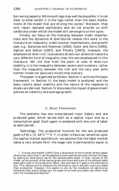
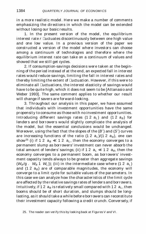

where
n (r ) 5 1 2s 1t
r 2 (r 2c)
is increasing in r whenever r (c2) thus in particular whens 2 (c2)
On the other hand if C( p) 5 (c(1 2 p)12 u )(1 2 u ) with u 1we have
(W)(L 1 W) 5 n (r) 5 1 2 t r (12 u ) u c1 u
which is decreasing in r so that 1 n (r) increases in r
Remark 1 If credit rationing was due to ex ante rather thanto ex post moral hazard (eg as formalized in Holmstrom andTirole [1997]) then n (r) would increase with r but one can showthat it will not increase too rapidly when the marginal efficiency ofeffort measured by the ratio of the increase in the probability ofsuccess over the effort cost required to achieve such an increase isnot too high The occurrence of cyclical (or volatile) growthpatterns will then be preserved
Remark 2 One can interpret the increasing relationshipbetween n and r in Holmstrom and Tirole [1997] as a wealth effectnamely the lower the interest rate r the higher the discountedvalue of future (ie end-of-period) prots and therefore the higherthe current borrowing capacity of investors Our microeconomicderivation of a constant multiplier 1 n eliminates this wealtheffect by introducing a second effect that offsets it exactly Namelya lower interest rate reduces the per dollar benet of lendersrsquo expost monitoring effort in collecting debt-repayment from theirborrowers This in turn reduces the maximum amount L whichlenders are willing to lend to borrowers with given current wealthW ie it reduces the credit multiplier 1 n Our choice of ex postmonitoring technology C( p) 5 2 c middot ln (1 2 p) generates a con-stant multiplier n by having the above two effects of r on investorsrsquoborrowing capacity exactly cancel out
Long-Term Debt Contracts
In this subsection we investigate the effects of introducinglong-term credit contracts into our basic model Intuitively along-term contract may allow borrowers to postpone a part of therepayment on their debt to periods when they expect to berelatively cash rich and thereby limit the variation in qt Here we
DUALISM AND MACROECONOMIC VOLATILITY 1393
ask whether such intertemporal substitution can eliminate thecycle we get in our basic model
Consider an extension of the above model where agents livefor two periods instead of one period but each new generation isonly born when the previous generation dies (ie it is a nonover-lapping generation model) For simplicity we also assume (a) thatin the absence of long-term lending the economy converges to atwo-cycle (b) that agents (borrowers and lenders) do not careabout consumption smoothing and therefore may as well consumeeverything at the end of their two-period life During a currentboom young borrowers might then be interested in signing atwo-period debt contract with their lending counterparts wherebya lsquolsquocurrentrsquorsquo rate r1 s 1 would be paid at the end of the rst periodand a future rate r2 s 2 would be paid at the end of the secondperiod Borrowers may also engage in further short-term borrow-ing during the second period
The borrowerrsquos incentive constraint at the end of the rstperiod will be
(A2) s 1(L1 1 W) 2 r1L1 $ s 1(1 2 t )(L1 1 W) 2 pr1L1
where L1 is the long-term debt contracted at the beginning ofperiod 1 and where r1(1 2 p) 5 c under the same monitoringtechnology as the one postulated in the above subsection
The above incentive-constraint can then be reexpressed as in(i) above namely
(A28) L1 5 ((1 n ) 2 1)W
where n 5 1 2 ( s 1t )cThe borrowerrsquos accumulated cash net of current debt repay-
mentmdashat the end of period 1mdashwill be equal to
W 5 s 1W 1 ( s 1 2 r1)L1
However the borrower will not be able to invest up to the amountW n simply because W does not reect his true wealth at thebeginning of period 2 Short-term lenders in period 2 will indeedtake into account the existence of further outstanding debt-repayment obligations toward long-term lenders
More formally if L2 denotes the additional amount to beborrowed short term in period 2 the borrowerrsquos incentive con-straint at the end of that period is written as
QUARTERLY JOURNAL OF ECONOMICS1394
(A3) s 1( s 1W 1 ( s 1 2 r1)L1 1 L2) 2 r2L2 2 r2L1
$ s 1(1 2 t )( s 1W 1 ( s 1 2 r1)L1 1 L2) 2 p2 middot r2 L2 2 p1r2 L1
where if we stick to the same debt-monitoring technology asbefore
(A4) r2(1 2 p2) 5 r2(1 2 p1) 5 c
Using (A4) to eliminate p1 p2 r2 and r2 in the incentive-constraint (A3) we end up reexpressing (A3) as
(A38) s 1W 1 ( s 1 2 r1)L1 1 L2 $ (c t s 1) (L1 1 L2)
Now if r1 5 0 (which corresponds to the best long-termcontract candidate for maximizing the borrowing capacity L2 andthereby possibly delaying the occurrence of a slump) the aboveincentive constraint becomes
L2 s 1W 1 ( s 1 2 (c t s 1))L1
(c t s 1) 2 1
Using (A28) to substitute for L1 we get
L2 V middot W
where
V 51
ns 1
1
n2
1
n2 1 5 b s
1
n2
1
n2 1
Whenever V s which in particular will be the case for bsufficiently small and n sufficiently close to 1 then it will still bethe case that investment capacity will grow at a lower rate thansavings grows in a boom so that even if we allow for long-termdebt contracts the occurrence of slumps will remain unavoidableHowever note that allowing for long-term debt contracts mayincrease the borrowerrsquos investment capacity as compared with thepure short-term borrowing case and yet not to a sufficient extentthat the occurrence of slumps can be avoided for example for nclose to 1
(1 n ) s 1W V middot W but still V s h
investment capacityunder short-term
borrowing
investment capacityunder long-term
bargaining
DUALISM AND MACROECONOMIC VOLATILITY 1395
APPENDIX 2 COMPARISON WITH THE GOODWIN MODEL
Here we show how our model can easily be extended in orderto offer a micro-founded version of Goodwinrsquos [1967] model ofgrowth cycles
Assume that the interest rate is permanently equal to r [[ s 1s 2] (if world capital markets were perfectly integrated r couldsimply be the world real interest rate) In order to generateuctuations in the prot share assume for simplicity a Leontiefproduction function Y 5 s min (KL) Assume that micro 5 0 (onlybusiness prots can be directly invested in production) and thatthe labor supply schedule is such that the wage rate v can takeonly two equilibrium values if v 5 v1 5 (1 2 b ) s then laborsupply (in efficiency units) grows at a rate n from the previousperiod and if v 5 v2 5 (1 2 b 8) s (with b 8 b and v2 v1) thenlabor supply grows at a rate n(1 1 a) (say that workers acceptworking extra hours if they are paid a higher wage)
It follows that if gt( 5 Kt Kt 2 1) n then vt 5 v1 W tB 5 gr middot
W t 2 1B with gr 5 (1 2 a )( b s 1 ( b s 2 r)((1v) 2 1) and gt1 1 5 gr
Conversely if gt n then vt 5 v2 W tB 5 g8rW t2 1
B with g8r 5(1 2 a )( b 8s 1 (b 8 s 2 r)((1v) 2 1) and gt1 1 5 g8r Therefore if weassume that g8r n gr n(1 1 a) there exists a two-periodcycle with g2t 5 g8r v2t 5 v1 and g2t 1 1 5 gr v2t 1 1 5 v2 boomscontain the seeds of their own destruction because the implied risein wage rates reduces businessesrsquo future ability to invest (andconversely for recessions) Unlike in our model the capital shareof output is countercyclical (it uctuates between b and b 8)However note that in both models the net-of-debt-paymentsprot share of capital income (and of output) is countercyclicaland it is the leading indicator of economic uctuations
UNIVERSITY COLLEGE LONDON AND EBRD LONDON
DEPARTMENT OF ECONOMICS MASSACHUSETTS INSTITUTE OF TECHNOLOGY
CEPREMAP AND CNRS PARIS
REFERENCES
Aghion P P Bacchetta and A Banerjee lsquolsquoCapital Markets and the Instability ofOpen Economiesrsquorsquo unpublished University College of London and HarvardUniversity 1998
Aghion P and P Bolton lsquolsquoA Trickle-Down Theory of Growth and DevelopmentrsquorsquoReview of Economic Studies LXIV (1997) 151ndash172
Attanasio O and G Weber lsquolsquoConsumption Growth the Interest Rate andAggregationrsquorsquo Review of Economic Studies LX (1993) 631ndash649
Banerjee A and A Newman lsquolsquoOccupational Choice and the Process of Develop-mentrsquorsquo Journal of Political Economy CI (1993) 274ndash298
QUARTERLY JOURNAL OF ECONOMICS1396
Benabou R lsquolsquoInequality and Growthrsquorsquo in NBER Macroeconomics Annual 1996(Cambridge MIT Press 1996) pp 11ndash74
Bernanke B and M Gertler lsquolsquoAgency Costs Net Worth and Business Fluctua-tionsrsquorsquo in Business Cycle Theory F Kydland ed (Cheltenham UK Ashgate1995a) pp 197ndash214
Bernanke B and M Gertler lsquolsquoInside the Black Box The Credit Channel ofMonetary Policy Transmissionrsquorsquo Journal of Economic Perspectives IX (1995b)27ndash48
Bernanke B M Gertler and S Gilchrist lsquolsquoThe Financial Accelerator in aQuantitative Business Cycle Frameworkrsquorsquo NBER Working Paper No 64551998
Eckstein O and A Sinai lsquolsquoThe Mechanisms of the Business Cycle in the PostwarErarsquorsquo in The American Business Cycle Continuity and Change R Gordon ed(Chicago University of Chicago Press 1986) pp 39ndash105
Fazzari S G Hubbard and B Petersen lsquolsquoFinancial Constraints and CorporateInvestmentrsquorsquo Brookings Papers on Economic Activity No 1 (1988) 141ndash195
Fazzari S and B Petersen lsquolsquoWorking Capital and Fixed Investment NewEvidence on Financial ConstraintsrsquorsquoRand Journal of Economics XXIV (1993)328ndash342
Feldstein M and C Horioka lsquolsquoDomestic Saving and International Capital FlowsrsquorsquoEconomic Journal XC (1980) 314ndash329
Fisher I lsquolsquoThe Debt-Deation Theory of Great Depressionsrsquorsquo Econometrica I(1933) 337ndash357
Frankel M lsquolsquoThe Production Function in Allocation and Growth A SynthesisrsquorsquoAmerican Economic Review LII (1962) 995ndash1022
Freixas X and J Rochet Microeconomics of Banking (Cambridge MIT Press1997)
Friedman B and K Kuttner lsquolsquoWhy Does the Paper-Bill Spread Predict RealEconomic Activityrsquorsquo in Business Cycle Indicators and Forecasting J Stockand M Watson eds (Chicago University of Chicago Press 1993a) pp213ndash249
Friedman B and K Kuttner lsquolsquoEconomic Activity and the Short-Term CreditMarkets An Analysis of Prices and Quantitiesrsquorsquo Brookings Papers on Eco-nomic Activity No 2 (1993b) 193ndash283
Galor O and J Zeira lsquolsquoIncome Distribution and Macroeconomicsrsquorsquo Review ofEconomic Studies LX (1993) 35ndash52
Goodwin R M lsquolsquoA Growth Cyclersquorsquo in C Feinstein ed Capitalism and EconomicGrowth (Cambridge Cambridge University Press 1967)
Haberler G Prosperity and Depression (London Allen and Unwin 1964)Harrod R lsquolsquoAn Essay in Dynamic Theoryrsquorsquo Economic Journal XLIX (1939) 14ndash33Holmstrom B and J Tirole lsquolsquoFinancial Intermediation Loanable Funds and the
Real Sectorrsquorsquo Quarterly Journal of Economics CXII (1997) 663ndash691Honkapohja S and E Koskela lsquolsquoThe Economic Crisis of the 1990s in Finlandrsquorsquo
unpublished Economic Policy Forum October 1998Keynes J The General Theory of Employment Interest and Money (New York
Harcourt and Brace 1936)Kiyotaki N and J Moore lsquolsquoCredit Cyclesrsquorsquo Journal of Political Economy CV
(1997) 211ndash248Piketty T lsquolsquoThe Dynamics of the Wealth Distribution and Interest Rate with
Credit Rationingrsquorsquo Review of Economic Studies LXIV (1997) 173ndash189Romer P lsquolsquoIncreasing Returns and Long-Run Growthrsquorsquo Journal of Political
Economy XCIV (1986) 1002ndash1037Stock J and M Watson lsquolsquoBusiness Cycle Fluctuations in U S Macroeconomic
Time Seriesrsquorsquo unpublished Harvard and Princeton Universities 1997
DUALISM AND MACROECONOMIC VOLATILITY 1397