Embed Size (px)
Citation preview

POLLACK PERIODICA An International Journal for Engineering and Information Sciences
DOI: 10.1556/Pollack.1.2006.1.2 Vol. 1, No. 1, pp. 5–34, (2006)
www.akademiai.com
DUCTILITY OF STEEL STRUCTURES: THE MODEL OF INTERACTIVE HINGE
Miklos IVANYI
Department of Structural Engineering, Budapest University of Technology and Economics, Bertalan Lajos u. 2, H−1111, Budapest, Hungary, e−mail: [email protected]
Received 10 June 2006; accepted 12 Augustus 2006
Abstract: Before the 1960s the ductility notion was used only for characterizing the material behaviour. After Baker’s research on plastic design, this concept has been extended to the structural level. This paper provides a general overview of ductility. The paper examines the behaviour of material ductility, cross−section ductility and member ductility separately, then it studies how the sum of the effects of all these ductilities affect the structural ductility. The effect of the different ductilities can be built into the structural behaviour through an interactive hinge model. The model of the interactive hinge also takes into consideration the effects of the residual stresses and deformations, the strain hardening and the plate buckling. Keywords: Ductility, Steel frame, Interactive hinge, Gable frame structure, Multi−storey frame structure
1. Introduction
1.1. Limit state design philosophy
The increasingly powerful experimental and computational tools of structural design require well−defined design philosophies. As the basis of the current design philosophy the concept of limit states [1] is seemingly accepted in many countries. The current design philosophy requires the estimation of the (fairly small) risk that the given structure is brought to its ultimate state (failure) and the (somewhat bigger) risk of the occurrence of a phenomenon restricting its regular use (serviceability). All this (excluding now brittle fracture and fatigue) necessitates the analysis of the structural
HU ISSN 1788−1994 © 2006 Akadémiai Kiadó, Budapest

6 M. IVANYI
response over a broad range of load levels, from working loads up to exceptionally high loads. As it is pointed out in the literature [2], in different periods of the engineering practice different importance was attributed to the two classes of limit states. In the earliest periods (e.g. in the works of Coulomb) − possibly inspired by the experience of collapsing vaults and breakdown of earthworks − interest was focused on the ultimate state and accordingly the applied methods of analysis could describe only the last phase of structural response. This methodology is still in use, for example in some branches of soil mechanics. A second period can be connected with the activity of the brilliant French scientist Navier, who seems to have been more interested in the second class of limit states. Quoting the preface of his 1826 book, which is of enormous influence on engineering practice [3]: “Knowing the cohesion, the ultimate load to be carried by a body can be determined. For the structural engineer, however, it is not sufficient to know the force great enough to cause breakdown of the body, but rather the load to be carried by the structure without causing in it changes progressing with time”. The concept of allowable stresses and the corresponding methods of analysis originates from this viewpoint: the “accurate” and simplified methods based on the theory of elasticity which were good enough to describe structural response at relatively low (working) load levels. The subsequent period is associated with the work of the Hungarian scientist Kazinczy, who is regarded as the initiator of plastic design of steel structures. In his early − and because of its language hardly accessible − paper (1914) on his tests with fixed−end beams he states [4]: “In the case of statically indeterminate steel structures there is a higher load than the load that is determined by the allowable stress (first yielding) and therefore the lower load value gives no information whatsoever about the margin of safety”. This indicates that the main interest was shifting again towards the first class of limit states, towards failure. Accordingly research was directed to complement the methods of analysis with new ones (based on the theory of plasticity among others) describing structural behaviour in the vicinity of and at the peak load, and often in post−failure phase as well. Thus the recent concept of limit states can be regarded as a balanced synthesis of the previous design philosophies complemented with the ductility phenomenon.
1.2. Leading role of ductility in limit state design
1.2.1. The definition of ductility
Before the 1960s the ductility notion was used only for characterizing the material behaviour. After the Housner’s studies of earthquake problems [5] and Baker’s research works on plastic design [6], this concept has been extended to the structural level. Following Baker’s work, in this paper the effect of the quasi−monotonic static loading system will be examined. In the practice of plastic design of structures, ductility defines the ability of a structure to undergo deformations after its initial yield, without any significant
Pollack Periodica 1, 2006,1

DUCTILITY OF STEEL STRUCTURES 7
reduction in the ultimate strength. The ductility of a structure allows us to predict the ultimate capacity of a structure, which is the most important criteria for designing structures under conventional loads. The following ductility types are widely used in the literature [7]:
• material ductility, or deformation ductility, which characterizes the material plastic deformations for different loading types;
• cross−section ductility, or curvature ductility, which refers to the plastic deformations of the cross−section, considering the interaction between the parts composing the cross−section itself;
• member ductility, or rotation curvature, when the properties of members are considered;
• structural ductility, or displacement ductility, which consider the overall behaviour of the structure.
A correlation among these types of ductility also exists.
1.2.2. Ductility for plastic design
The plastic behaviour of a structure depends upon moment redistribution. The attainment of the predicted collapse load is related to the position of plastic hinges, where sections reach the full plastic moment, and to the plastic rotation which other hinges can develop elsewhere. Hence, a good behaviour of a plastic hinge requires a certain amount of ductility, in addition to its strength requirement. The plastic rotation capacity is the more rational measure of this ductility. The basic requirement for plastic analysis of statically indeterminate structures is that large rotations (theoretically infinite) are possible without significant changes in the resistant moment. But these theoretical large plastic rotations may not be achieved because some secondary effects occur. The plastic rotation is usually limited by flexural−torsional instability, local buckling or brittle fracture of members. Due to the reduction of the plastic rotation, cross−section behavioural classes are used in the design practice (Fig. 1a). EUROCODE 3 defines the following classes:
Fig. 1. Cross sectional, member and frame behaviour classes
Pollack Periodica 1, 2006, 1

8 M. IVANYI
• class 1 (plastic sections); sections belonging to class 1 are characterized by the capability to develop a plastic hinge with high rotation capacity;
• class 2 (compact sections); class 2 sections are able to provide their maximum plastic flexural strength, but they have a limited rotation capacity, due to some local effects;
• class 3 (semi−compact sections); sections fall into this class when the bending moment capacity for the first yielding can be achieved without reaching the plastic moment;
• class 4 (slender sections); sections belonging to this class are not able to develop their total flexural resistance due to the premature occurrence of local buckling in the compressed parts.
Evidently, only the first two classes have sufficient ductility to assure the plastic redistribution of moments. This classification is limited to the cross−section level only, so it has many deficiencies. Another more effective classification at the level of a member has been proposed by Galambos and Lay [8] as shown in Fig. 1b:
• ductility class HD (high ductility) corresponds to a member for which the design, dimensioning and detailing provisions are such that they ensure the development of large plastic rotations;
• ductility class MD (medium ductility) corresponds to a member designed, dimensioned and detailed to assure moderate plastic rotations;
• ductility class LD (low ductility) corresponds to a member designed and dimensioned according to general code rules which assures low plastic rotations only.
An effective classification at the level of a frame considering the spacing and efficiency of lateral support has been proposed by Ivanyi [9] as shown in Fig. 1c:
• ductility class 1: full support corresponds to a frame for which the design, dimensioning and detailing provisions are such that they ensure the development of the plastic carrying capacity with large plastic rotations;
• ductility class 2: adequate support that ensures the development of the plastic carrying capacity without plastic rotations;
• ductility class 3: sufficient support, which ensures the development of the elastic carrying capacity;
• ductility class 4: poor lateral support under the elastic carrying capacity.
1.3. Difficulties in predicting failure
In contrast to the expectation of the initiators of plastic design, the analysis of structural response in the vicinity of the peak load proved to be extremely complicated, due not only (and even not mainly) to the inelastic behaviour, but to the fact that in the vicinity of the peak load
Pollack Periodica 1, 2006,1

DUCTILITY OF STEEL STRUCTURES 9
• changes in the geometry (geometrical non−linearity) gain importance over other factors because the effect of initial geometrical imperfections (often negligible at lower load levels) is magnified;
• residual stresses (remaining latent at lower loads) interact with growing active stresses resulting in premature plastic zones; and last but not least;
• the usual and widely accepted tools of analysis, e.g. the beam theory based on the Bernoulli−Navier theorem or the small−deflection theory of plates, restricting the actual degree of freedom of the structure, cannot describe exactly the real response of the structure at failure.
These difficulties can be overcome in the case of simple structural elements (separated compression members, parts of plate girders, etc.) by using more refined methods, for example the finite element method or considering degrees of freedom (e.g. distortion of cross−sections) that are excluded from traditional analysis. The difficulties can also be avoided in the case of statically determinant structures, where the above−indicated complex behaviour is usually confined to a limited section of the whole structure. If the simplified model is not elaborate enough to reflect real structural behaviour, a secondary, more detailed, local model or “target” model is inserted to depict the mostly critical part of the structure. In this way more realistic quality parameters (and limit surface) can be deduced from the primary parameters that are already known [10]. Because of the interaction of the local and the global behaviour, there is a larger problem in the case of hyper−static structures, as the additional information gained by the secondary local model cannot be fed back to the computation of the primary parameters. Furthermore, if − as happens very often − the secondary model can be analysed by numerical methods or only experimentally, but the results have to be either re−interpreted to gain mathematically treatable, sufficiently simple rules, or the secondary model has to be simplified to furnish digestible results. In both cases the validity or accuracy has to be proved by failure tests with full−scale structures (which are usually very expensive). The same difficulties apply to quantities which cannot be measured directly or which are hardly measurable, such as residual stresses.
1.4. The role of the softening phenomenon
When studying the effect of the softening phenomenon it should be kept in mind that the load−displacement diagram of the structure may be of an ascending type even if the given member section or semi−rigid connections are of a descending type. In the theory of plasticity, when deriving the condition of plasticity or some other physical relationships, Drucker’s postulate for stability is applied, by assuming stable materials [11]. It should be noted that Drucker’s postulate is not a natural law but a criterion for classification [12]. Materials very often do not correspond to the assumptions of stable materials, or structural elements may behave in an unstable way, while at the same time their material is of a stable state. Maier [13] was one of the first to treat the problem of the effect of the unstable state of certain members when he studied the behaviour of a triangular shaped structure.
Pollack Periodica 1, 2006, 1

10 M. IVANYI
Later it was Maier again who in 1966 re−introduced the subject and investigated a structure consisting of compressed members and rigid beams where load−displacement diagram of individual members contained stable and unstable parts. Maier and Drucker [14] re−examined the original Drucker’s postulate since the original postulate is suitable for the determination of the convexity and normality of the condition of plasticity in the case of stable materials only. When studying the load bearing capacity of steel structures, the problem of unstable material or softening material, according to Drucker’s postulate does not appear since the strain−hardening of the steel material may increase in a major way over the plastic load bearing capacity of steel structure. However, as it has been known for a long time, the final collapse of steel structures is caused − in a high percentage of cases − by instability (plate buckling, flexural−torsional buckling), or semi−rigid phenomena that may occur in the cross section or in a structural joint (Fig. 2).
Fig. 2. Behaviour of a simple structure
Concerning steel structures the properties of plastic hinges over and above the usual elastic−ideally plastic−hardening behaviour may be complemented with the effect of instability (flexural−torsional buckling) developing in the given structural unit (environment of the plastic hinge), or in the periphery of semi−rigid connections. This type of inelastic or interactive hinge describes the behaviour of the structural unit and at the same time, also satisfies the criteria of unstable or softening structural unit, according to the Maier−Drucker’s postulate. When determinig the plastic load bearing capacity of steel structures the softening has not been considered or applied so far. The effects of the stability phenomena
Pollack Periodica 1, 2006,1

DUCTILITY OF STEEL STRUCTURES 11
causing the softening character (flexural−torsíonal buckling, plate buckling, semi−rigid connections) can be taken into account indirectly with the aid of construction rules. In principle, mathematical programming allows the investigation of more complex steel structures too, however, it is less suitable for designing practice. Ivanyi [15] has suggested a procedure that takes into account the softening character of the inelastic hinge in the form of an interactive zone. The softening character of the interactive zone is caused by the buckling of the component plates, a phenomenon that can be studied with the help of the yield mechanism. The purpose of this article is to describe 1) how the load−deflection curve of frames may be constructed in as exact a manner as possible and 2) to describe approximate methods whereby the load−deflection curve, and particularly the limit point load, can be estimated with the softening phenomenon.
2. Investigation of plate buckling with the aid of yield mechanism
In the course of plate experiments, if the thickness/width ratio is small the plate does not lose its load−bearing capacity with the development of plastic deformations but is able to take further (small increase in) load up to the point where the deformation capability is exhausted. In the course of the loading process “crumplings” (buckling) can be observed on the plate surface. These “crumplings” are formed by a yield mechanism, with the plastic moments acting in the plastic hinges (peaks of waves) not constant but ever increasing due to strain−hardening. The yield mechanism performed by “crumplings” can be extended to the component plates of the bar. The description of the behaviour of the yield mechanism is obtained from the extreme−value theorems of plasticity with the aid of the theorem of kinematics. Thus, in the course of our investigations, an upper limit of load bearing capacity can be determined. However, to be able to assess the results, the following have to be considered: the yield mechanisms are taken into account through the “crumpling” forms determined experimentally; and on the other hand, the results of the theoretical investigations are compared with the experimental ones.
2.1. Yield mechanism forms based on experimental results [16, 17]
The different forms of yield mechanisms can be determined on the basis of experimental results. The yield mechanism forms of an I−section bar can be classified according to the following critieria.
a) According to the way of loading; b) According to the positions of the intersecting lines of the web and the flanges, the
so−called “throat−lines”; thus; i) the evolving formation is called a planar yield mechanism if the two
“throat−lines” are in the same plane after the development of the yield mechanism;
Pollack Periodica 1, 2006, 1

12 M. IVANYI
ii) the evolving formation is called a spatial yield mechanism if the two “throat−lines” are not in the same plane after the development of the yield mechanism.
2.1.1. Constant bending moment along the bar axis
a) Planar yield mechanism: The buckled form of the bent specimen and the chosen yield mechanism formation are shown in Fig. 3a. As an effect of moment M, a rotation θ develops furthermore tension and compression regions appear. The symbol of the yield mechanism is (MC)P, where C stands for the constant bending moment. b) Spatial yield mechanism: The form of the spatial yield mechanism in the case of a bent beam is shown in Fig. 3b. The beam ends are assumed to be hinge−supported in both main inertial directions. The yield mechanism models the buckling of the component plates of the bent members, the lateral buckling of the beams as well as their interaction. The symbol of this yield mechanism is (MC)S.
(MC)P (MC)S
a) b)
Fig. 3. Planar a) and spatial b) yield mechanisms of an I−beam with constant bending moment along the member axis
2.1.2. Varying bending moment along the bar axis
In the case of a varying bending moment along the member axis, it is assumed that the “crumplings” of the web plate of the I−section in the cross−section of the concentrated force is hindered by the thickness of the web plate or by the ribs. Climenhaga and Johnson [18] assumed yield mechanism forms for the steel beam part of a composite steel−concrete construction, which are similar to those introduced in this paragraph.
Pollack Periodica 1, 2006,1

DUCTILITY OF STEEL STRUCTURES 13
a) Planar yield mechanism: The buckled form of a bent specimen and the selected yield mechanism are shown in Fig. 4a. As an effect of the moment, a rotation θ develops and because of the clamping of the cross−section EC, the yield mechanism loses its symmetric character. The symbol of the yield mechanism is (MV)P where V stands for the varying moment. b) Spatial yield mechanism: The form of the spatial yield mechanism in the case of a varying bending moment along the beam axis is shown in Fig. 4b. As an effect of the moment, a rotation θ develops. The symbol of the yield mechanism is (MV)s.
P J Q
H K
N G M
CB
D
A
F E
θ
(MV)P (MV)S
a) b)
Fig. 4. Planar a) and spatial b) yield mechanism of an I−beam with varying bending moment along the member axis
2.1.3. Yield mechanism of the component plates of an I−section member
Yield mechanism formations have been determined for different stresses. On the basis of the experimental results it is expedient to decompose these yield mechanism formations into the yield mechanism formations of the component plates of an I−section beam, as certain yield formations are common considering all yield mechanisms. Fig. 5 shows the yield mechanisms of the component plates where F is the flange plate, W is the web plate; the odd numbers refer to the planar yield mechanisms and the even numbers to the spatial yield mechanisms. To classify the yield mechanisms of component plates, the following groups has been identified:
a) Flange plate, if the plate is supported along one line; b) Web plate, if the plate is supported at the unloaded ends;
bi) axial forces and bending (W−1)−(W−6); bii) transverse forces transmitted directly through the web (W−11−12−13); bii) transverse forces only on one side of the web panel (W−21−22−23); biii) tension fields on the web panel (W−30; W−40).
Pollack Periodica 1, 2006, 1

14 M. IVANYI
Fig. 5. Yield mechanisms of the component plate elements of an I−section member and
beam−to−column joints
2.1.4. Yield mechanism of joint configurations
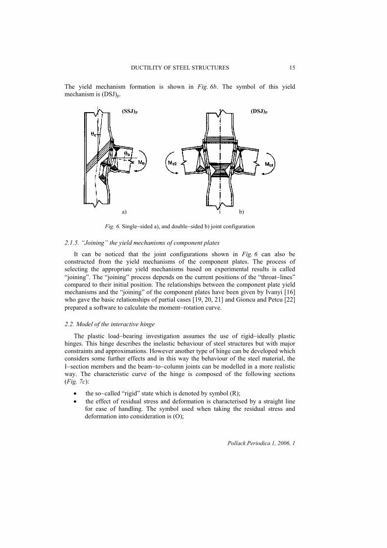
Yield Mechanism of Single−Sided Joint Configurations. The main sources of deformability of joint configurations which must be contemplated in a beam−to−column joint (Fig. 6a) are:
• the connection deformability Mb−θc characteristic; • the column web panel shear deformability VWp−γ characteristic; • the local buckling of the column web panel.
In the case of the yield mechanism formations shown in Fig. 6a, the effect of the local buckling of the beam cross−section, the local yield of the column web panel caused by shear and the effect of patch loading has also been taken into account. The symbol of this yield mechanism is (SSJ)P. Yield Mechanism of Double−Sided Joint Configurations. The main sources of deformabilíty of joint configuration which must be contemplated in a beam−to−column joint (Fig. 6b) are:
• the left hand side connection deformabílíty Mb1−θc1 characteristic; • the right hand side connection deformability Mb2−θc2 characteristic; • the column web panel shear deformability Vwp−γ characteristic; • the local buckling of the column web panel.
Pollack Periodica 1, 2006,1
DUCTILITY OF STEEL STRUCTURES 15
The yield mechanism formation is shown in Fig. 6b. The symbol of this yield mechanism is (DSJ)p.
(SSJ)P (DSJ)P
a) b)
Fig. 6. Single−sided a), and double−sided b) joint configuration
2.1.5. “Joining” the yield mechanisms of component plates
It can be noticed that the joint configurations shown in Fig. 6 can also be constructed from the yield mechanisms of the component plates. The process of selecting the appropriate yield mechanisms based on experimental results is called “joining”. The “joining” process depends on the current positions of the “throat−lines” compared to their initial position. The relationships between the component plate yield mechanisms and the “joining” of the component plates have been given by Ivanyi [16] who gave the basic relationships of partial cases [19, 20, 21] and Gioncu and Petcu [22] prepared a software to calculate the moment−rotation curve.
2.2. Model of the interactive hinge
The plastic load−bearing investigation assumes the use of rigid−ideally plastic hinges. This hinge describes the inelastic behaviour of steel structures but with major constraints and approximations. However another type of hinge can be developed which considers some further effects and in this way the behaviour of the steel material, the I−section members and the beam−to−column joints can be modelled in a more realistic way. The characteristic curve of the hinge is composed of the following sections (Fig. 7c):
• the so−called “rigid” state which is denoted by symbol (R); • the effect of residual stress and deformation is characterised by a straight line
for ease of handling. The symbol used when taking the residual stress and deformation into consideration is (O);
Pollack Periodica 1, 2006, 1

16 M. IVANYI
• strain−hardening is one of the important features of the steel material, therefore the characteristic curve contains a section denoted by (S);
• the effect of “crumpling” of different plate elements is taken into account by a section indicated by (L).
AD Q
Cθ
m
Mpl
Mpl
MH
M
Cxh
fy
θH θ
σ
ε
E / K = E= =
(R)
(O)
(S)(L)
(a) (b)
(c)
Fig. 7. Model of interactive hinge
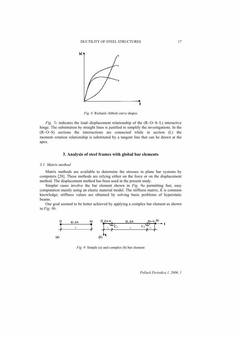
The models that take the above effects into consideration in the investigation of load−displacement (relative displacement) relationships are called “interactive” models. Some alternative empirical models, such as the exponential model [23], the Ramberg−Osgood model [24] and the Richard−Abbott model [25, 26] have been widely used to represent the nonlinear moment−rotation of members and semi−rigid connections. The ability of the Richard−Abbott function to model characteristics, as shown in Fig. 8, which exhibit strain hardening (a), strain softening (b), as well as strain stiffening (c) behaviours, makes it very useful in the analysis of steel structures however the present study introduces the piecewise linear model to describe the moment rotation. The model of the interactive hinge taking into consideration the effect of the rigid state, the residual stress, he strain−hardening and the plate crumplings can be described with the aid of the “equivalent beam length” suggested by Horne [27] (Fig. 7a). The material model employed in the investigations is shown in Fig. 7b. The effect of the residual stresses and deformations is substituted by a straight line. The effect of strain−hardening can be determined with the help of the rigid−hardening (R−S) model. The buckling of the I−section member component plates is described by the yield mechanism curve, which is substituted by a straight line.
Pollack Periodica 1, 2006,1
DUCTILITY OF STEEL STRUCTURES 17
Fig. 8. Richard−Abbott curve shapes
Fig. 7c indicates the load−displacement relationship of the (R−O−S−L) interactive hinge. The substitution by straight lines is justified to simplify the investigations. In the (R−O−S) sections the intersections are connected while in section (L) the moment−rotation relationship is substituted by a tangent line that can be drawn at the apex.
3. Analysis of steel frames with global bar elements
3.1. Matrix method
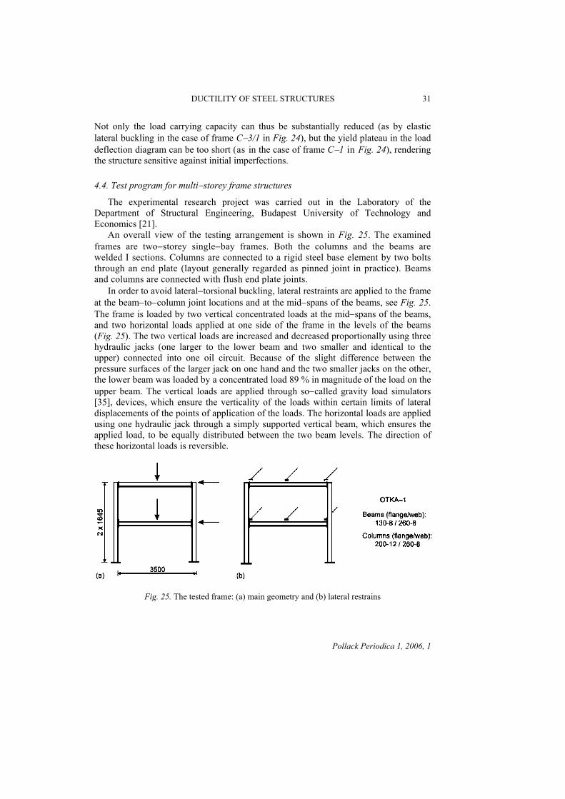
Matrix methods are available to determine the stresses in plane bar systems by computers [28]. These methods are relying either on the force or on the displacement method. The displacement method has been used in the present study. Simpler cases involve the bar element shown in Fig. 9a permitting fast, easy computation mainly using an elastic material model. The stiffness matrix, K is common knowledge; stiffness values are obtained by solving basic problems of hyperstatic beams. Our goal seemed to be better achieved by applying a complex bar element as shown in Fig. 9b.
Fig. 9. Simple (a) and complex (b) bar element
Pollack Periodica 1, 2006, 1

18 M. IVANYI
The two end parts of the bar, of lengths l1 and l2, are infinitely rigid (maybe l1 = l2 = 0); the middle part is elastic. Rigid and elastic parts of the bar are connected by rotational springs. Each of the springs is able to rotate only in the plane of the structure. Stiffnesses, i.e. spring constants are c1 and c2 [29]. Details of the method that gives the connection between the unit end deformations and the relevant stress resultant can be found in the literature [17]. Spring characteristics have the general form as shown in Fig. 7 and it models an interactive hinge. Sections have different spring constants c = ∆M / ∆θ indicating the given section of the elasto–plastic behaviour or of the stability condition of the bar. The characteristics are strictly monotonous for θ but not for M. Namely there is a peak followed by a descending path of the curve.
3.2. Simple approximate method
Numerous approximate engineering methods are introduced in the literature [30], from which as one of the possibilites we are going to deal with the extension of the Mechanism Curve Method. The Mechanism Curve Method − besides the determination of the plastic load bearing capacity − can take into consideration the effect of finite deformations and strain hardening of steel.
3.2.1. Mechanism curve method
Horne [27] proposed the use of the simple rigid−plastic−rigid relationship in order to take into account the effect of strain−hardening on the collapse load of a structure. The change of the geometry due to elasto−plastic deformations tends to decrease the ultimate load bearing capacity of steel frames in comparison with the plastic collapse load. This tendency is counteracted by the strain−hardening properties of steel. The rigid−plastic−rigid theory of structural behaviour is found to be an adequate mean to assess the stiffness of a structure immediately when the last hinge is formed in a plastic hinge mechanism. Different strain−hardening theories can be used during the analysis (Fig. 10):
• rigid−plastic−rigid (RPR) model [27]; • rigid−plastic−hardening (RPH) model [31]; • rigid−hardening (RH) model.
Fig. 10. Strain−hardening models
Pollack Periodica 1, 2006,1

DUCTILITY OF STEEL STRUCTURES 19
This study uses the rigid−hardening (RH) hinge model and in this case the rigid−plastic work equation [16] becomes
( jj
jpji k
kkkii mMLNuQ θφλ ∑ +=⎟⎟⎠
⎞⎜⎜⎝
⎛∑ ∑+ 2 ) . (1)
3.2.2. Approximate engineering method to take into consideration the effect of plate buckling [16]
We extend the category of hardening plastic (RH) hinges by taking the effect of plate buckling into consideration. Such hinge model can be the basis of an Approximate Engineering Method that − without analysing the full load history − with simple methods can directly take the effect of plate buckling into consideration. Fig. 7c shows the linear interaction of moment−rotation of the interactive hinge that contains the effects of strain−hardening and plate buckling. The essence of the Approximate Engineering Method is that the two effects are separated and the interactive hinge of the structure is put together from two separate components as shown in Fig. 11:
• Strain−hardening component: (S); • Plate buckling component: (L).
With the assumed two hinge components the values of the load parameter for the chosen mechanism of the framework can be determined as a function of finite deformations. The strain−hardening component of Eq. (1) is
( ) ∑ ∑+=∑ ∑+ θθφλ SpS mMNLQu 2)( , (2)
∑ ∑+
∑ ∑+=
2)( φ
θθλ
NLQumM Sp
S . (3)
θθ θ
Mpl Mpl
M' = M + Mpl ∆
M'
mSmL
M
(S)(L)
θ
M
∆M
Fig. 11. Separated components of interactive hinge
To write down Eq. (1) for the plate−buckling component it should be assumed that the interactive hinge characteristic curve contains the rigid and the plate buckling effects.
Pollack Periodica 1, 2006, 1

20 M. IVANYI
The rigid curve section goes up to the value of M' = MP + ∆M first, then a linearly decreasing change is taken into consideration due to the effect of plate buckling. Because of the section of the characteristic curve belonging to the plate−buckling component, external and internal capacities and works are written similarly to Eq. (2), except the sign of the increment m θ
( ) ∑ ∑−′=∑ ∑+ θθφλ LL mMNLQu 2)( , (4)
∑ ∑+∑ ∑−′
=2)( φθθλ
NLQumM L
L . (5)
Load parameter λ(S) takes into consideration the effect of strain−hardening, while load parameter λ(L) includes the effect of plate buckling. From the displacement given by the intersection of the two curves; the reductionlike change of state is due to the effect of plate buckling as shown in Fig. 12. In connection with the results it should be emphasized, that − similarly to the plastic load bearing capacity analysis − the expression−taking the two separate components into consideration−assumes the structure motionless till the moments MP and M' in the hinges form.
θ
λ
θ*
(S) (L)
λL0
0Sλ
Fig. 12. Load parameter and displacement curve
3.3. The case of the “direct method of design”
Halasz [34] used previously the “direct method of design” for the frame with elastic−ideally plastic hinges and ideal rigid or hinge connection model.
3.3.1. First and second order approach
The analysis of the behaviour of elasto−plastic frames neglecting the change in the geometry of the structures while setting up the equations of equilibrium is referred to as first order approach. The steel frame has normal plastic hinges, semi−rigid connections and column bases at the respective locations. The load−deflection diagram of the frame shown in Fig. 13 according to the first order approach F0
(I) can be expressed as
Pollack Periodica 1, 2006,1

DUCTILITY OF STEEL STRUCTURES 21
, (6) ( RdplI MMfF ;)(
0 = )where Mpl is the plastic moment of the cross section and MRd is the moment resistance of the semi−rigid connection or column base.
Fig. 13. First and second order approach
In the second order approach the equilibrium equations are set up in such a way that they take into account the deflections of the structure. A typical load−deflection diagram according to the second order approach F0
(II) is illustrated in Fig. 13.
, (7) ( jRdplII SMEIMfF ;;;)(
0 = )where Mpl is the plastic moment of the cross section, EI is the elastic stiffness of the cross sections, MRd is the moment resistance and Sj is the rotational stiffness of the semi−rigid connection or column base. The second order load−deflection curve differs basically from the curve based on the first order approach as follows: i) the branches are curvilinear; ii) the failure load (or peak load) is lower than in the case of the simple plastic (first order) theory; iii) the failure may occur before the complete yield mechanism has developed and is followed by unstable behaviour. In addition, the location and sequence of occurrence of the generalized hinges do not necessarily coincide with those determined in the case of first order theory.
3.3.2. Direct method of design
Let a frame − such as the one shown in Fig. 13 − be subject to monotonously increasing loads proportional to a single load factor F. For simplicity we confine our
Pollack Periodica 1, 2006, 1

22 M. IVANYI
investigation to cases when the axial forces can be expressed in the form of Nk = βk·F , where parameter βk is constant. The frame may be built up of perfectly elastic members and generalized hinges at certain locations. The load−deflection curve can be characterised by the diagram shown in Fig. 14. The subsequent branches of the curve indicate the behaviour of the frame containing an increasing number of generalized hinges [32]. Each branch continued beyond its range of validity (dashed lines in Fig. 14) approaches asymptotically a certain value Fcr,n . These values are referred to in the literature as “deteriorated critical loads” (Horne and Merchant [33], Halasz [34]). They represent the load factor causing buckling of a frame in a completely elastic state. During the analysis, the generalized hinges developed in the frame have been replaced with real hinges.
Fig. 14. Load displacement curve
According to the first order approach, the failure load depends upon the value of the generalized moment only. In a second order approach, however, failure load depends upon two types of quantities: the moment resistance of the cross sections or the semi−rigid connections (i.e. the “strength” of the structure), and the flexural stiffness of the cross sections (EI) or the rotational stiffness of the semi−rigid connections or colunm bases (i.e. the “rigidity” of the structure). Assuming EI and Sjoint to increase infinitely, the concept of rigid−plastic material can be derived. In this case failure will only occur after the formation of a complete yield mechanism, however by studying Fig. 15 two frame types can be distinguished:
• “relatively rigid” frame: the failure should take place when the number of generalized hinges has reached the number of hinges necessary for the complete mechanism, thus i = n ;
• “relatively flexible” frame: the failure load is reached in the presence of a lower number of generalized hinges than the number of hinges that transforms the structure into a complete mechanism (i < n).
Pollack Periodica 1, 2006,1

DUCTILITY OF STEEL STRUCTURES 23
Fig. 15. Relatively rigid and relatively flexible frames
A special but easy to handle case of the “Direct Method of Design” is to design a structure where the predetermined failure load FF coincides with one of the “deteriorated critical loads” Fcr,n . Fig. 16 represents a case with n = 3, i.e. the structure fails as soon as the third generalized hinge has developed.
Fig. 16. Illustration of the “Direct Method of Design”
4. Evaluation of load bearing and ductility capacity of steel frames
4.1. Test program for gable−frame structures
The experimental research project was carried out in the Laboratory of the Department of Steel Structures, Technical University of Budapest. Two main series of experiments were covered by the test program.
Pollack Periodica 1, 2006, 1

24 M. IVANYI
The first part of the program contained the additional tests on stub columns, frame corners, plate elements, simple beams [35]. A brief summary of this series is given in Fig. 17.
Fig. 17. First part of the test program
4.1.1. Full−scale tests of frames
In the second part of the program the full−scale tests of frames have been carried out. Fig. 18 gives a brief summary of the full−scale tests and dimensions of the specimens, indicating the loads and the characteristics of the loading process [35]. Test frames had rafters with a slope of 30 % (16.7°), welded column sections. Rafter−to−column and mid−span connections have been end−plated ones with high−strength prestressed bolts. Different types of lateral supports were applied to the frames to prevent or decrease out−of−plane displacements and/or rotations of selected sections. Vertical loads at the purlin supports were applied to the upper flange of rafter, so web and bottom flange were not restrained laterally. To make horizontal displacement (sidesway) unrestricted, jacks were fastened not directly to the floor−slab, but through a so−called gravity load simulator (Fig. 19). The simulator consists of three elements: two bars and a rigid triangle. The two bars had pin−joints at both ends resulting in a one−degree−of−freedom mechanism. Hydraulic jacks were joined to the rigid triangle. This mechanism produced a vertical load acting upon the intersection of the two bar axes. Characteristics curve of the simulator illustrating the ratio of horizontal and vertical load component as a function of the horizontal displacement is shown in Fig. 19c. A remark in connection with the characteristics of the loading seems to be rather important. During the mathematical (theoretical) investigations, virtual disturbances have been assumed for the equilibrium state analysis of the structure so that these disturbances do not influence loading [36]. However, in the case of experimental investigations, these disturbances are, quite naturally, real ones thus their effect does not only manifest itself on the structure but also in the loading system. Therefore the
Pollack Periodica 1, 2006,1

DUCTILITY OF STEEL STRUCTURES 25
interaction of the structure and the loading system has also to be determined during the experimental investigations.
120006000 6000
a
hr
φ
b s
C–2C–1
C–3/2 B–1/2C–3/3 B–1/3C–3/4 B–1/4C–3/1 B–1/1P
P
P
P P P P
P
V V V
V
VV
P
V
Proportional load
Variable repeated load
Hinged base frames Fixed base frames
Crane load (heavy)
Crane load (light)
Fig. 18. Second part of test program
First of all it should be noted, that a large amount of steel structures in the engineering practice are loaded with dead or gravity load. The characteristic curves of gravity loading are horizontal lines. The highest characteristic line corresponding to the highest gravity load is tangential to the load−displacement curve and it touches the load−displacement curve at the peak of the curve. This peak point also indicates the loss of stable equilibrium state. However, this general observation has become a hindrance to the cognitive process, since, on the basis of the above observation, not only the complete structure but also individual structural elements have been analysed experimentally mainly for gravity load. These analyses may have “given” basis to the statement that no stability loss of the structural elements could take place prior to the development of global stability loss. However should the stability loss of the structural element occur it means the collapse, loss of stability of the complete structure. This train of thought eliminated major problem spheres from the program of theoretical and experimental investigations. In the course of our investigations and analyses it was first the experimental results that indicated and then proved very convincingly that this type of viewpoint simplifies the behaviour of the structure.
Pollack Periodica 1, 2006, 1

26 M. IVANYI
Gravity load Hydraulic jack
Hinge
Point of action
Central positionSwayed position
Pv [%]P
Pv
–1,6
0
0,2
P
∆
LrH
d
d=r=
H=L=
259,8mm300mm
1100mm564mm
250Sidesway [mm]∆
Fig. 19. Gravity load simulator
A full knowledge of the behaviour of the structure also involves the knowledge of the behaviour of structural elements and thus it is not only a demand from the viewpoint of “comfort” that when investigating the supporting structures also the descending section of the load−displacement curve should be considered, but this is also required by the demand of a complete knowledge. The relationship of the loading characteristics and the model of supporting structure can be seen for a simple model in Fig. 20a. The state indicated in Fig. 20b develops as an effect of gravity load type loading. The state shown in Fig. 20c − taking also into consideration the descending section of the load−displacement curves of individual units − develops as an effect of deformation type loading. The maximum load capacity characterizes the behaviour of the structure sufficiently well so the use of deformation−type loading is not absolutely necessary in this case. However, it is expedient to carry out the standard experiments for structural elements, beams, columns, connections, column bases, etc. first and foremost with deformation−type loading if both the ascending and descending parts of the load−displacement curve are to be considered and if the displacement capability of the supporting structures is to be determined.
4.1.2. Test of frame C−3/2
The load−deflection diagram is shown in Fig. 21. Failure was due to plate buckling in the plastic hinge below the haunch in the column (to develop the earliest) and
Pollack Periodica 1, 2006,1

DUCTILITY OF STEEL STRUCTURES 27
lateral buckling around the midspan. Load−deflection diagram proves the formation of the predicted yield mechanism.
Fig. 20. Effect of behaviour of loading system
4.2. Results of theoretical and experimental investigations for gable−frame structures
4.2.1. Application of computer programs
The load−deflection curve for the experimental frame C−3/2 is shown in Fig. 21. On the side of the horizontal load, the first inelastic hinge develops due to the residual stresses and deformations in the cross section beneath the frame knee and this hinge develops at 52 % of the maximal frame load. At 97 % of the maximal load, Zone (L) describing the effect of plate buckling develops also in this cross section, i.e. in the frame cross section an “unstable” state − a descending characteristic curve − develops. For comparison Fig. 21 also introduces the characteristic load−displacement curve of the frame structure in the case when the basis of the computations is the traditional plastic hinge. The results show well that the presence of residual stresses influences in a major way the range of limited plastic deformations, however, mainly because of the cross section geometry of the experimental beam, the maximal load bearing capacities computed with the traditional (elastic−ideally plastic) hinge as well as those obtained by the interactive hinge coincide with the experimental results.
4.2.2. Application of the approximate engineering method
The Approximate Engineering Method is presented for test frame C−3/2. The column base of the test frame was supported by the foundation, but it did not act as a fix end, so plastic load bearing capacity of the column base was determined by experiments. These values were used in the calculations.
Pollack Periodica 1, 2006, 1

28 M. IVANYI
The Approximate Engineering Method is suitable for the analyses of the strain hardening and to take into the effect the plate buckling. The most important steps of the analysis of frame C−3/2 given in Fig. 21 are as follows:
Fig. 21. Experiment (continuous line) and analysed (dashed) result for gable frame structure
• plastic load bearing capacity analysis by a mechanism chosen according to the test results;
• analysis of effects of finite deformations with the help of the chosen mechanism;
Pollack Periodica 1, 2006,1

DUCTILITY OF STEEL STRUCTURES 29
• effect of strain−hardening: moment−rotation relationship of inelastic zones can be replaced by straight lines, therefore rigid−hardening model can be applied to determine mS;
• effect of plate buckling: characteristic curves of interactive hinges can be replaced by straight lines too, therefore the rigid−hardening model can be applied to determine M’ and mL..
Fig. 21 compares the test result and the results of the Approximate Engineering Method taking into consideration the strain−hardening of steel and the effect of the plate buckling. The comparison shows that the Approximate Engineering Method gives a satisfactory result for the maximum loads and the unstable equilibrium state path of the whole structure as well. At the same time the analysis can be done at the “desk of the designer”.
4.3. Analysis of the influence parameters for gable−frame structures
4.3.1. Column bases
Column bases were fixed or hinged. The hinges were not ideal: columns have been supported by large base−plates. Fig. 22 compares the measured bending moment due to vertical and horizontal load with the calculated ones assuming pinned (dashed line) and fixed (solid line) frames. Fig. 23 shows the corresponding moment−rotation diagrams for the pinned and fixed frames. Moreover Fig. 23 also shows the experimental results, which fall between the theoretical bounds. However this curve is identical to the curve, which can be obtained by using an interactive hinge method.
Fig. 22. Measured and calculated bending moments
4.3.2. Lateral supports
Spacing and efficiency of lateral supports proved to be of basic importance. Their effect is illustrated in Fig. 24. The importance of adequate spacing of lateral supports and their efficiency in preventing the rotation of the cross section around the bar axis has to be emphasized as purling and rails connected to tension flanges often cannot be regarded fully effective in the case of thin webs.
Pollack Periodica 1, 2006, 1

30 M. IVANYI
Fig. 23. Effect of column−bases for the behaviour of gable−frame structure
50 150100 200 300250 e [mm]
1,0
0,5
4800
310041
60 C–3/1
C–3/1
C–1
C–1
C–3/2
C–3/2
C–2
C–2
Calculated carrying capacity
ee
Lateral supports
P/Py
0,85
1,03
1,111,17
Fig. 24. Effect of lateral supports
Pollack Periodica 1, 2006,1
DUCTILITY OF STEEL STRUCTURES 31
Not only the load carrying capacity can thus be substantially reduced (as by elastic lateral buckling in the case of frame C−3/1 in Fig. 24), but the yield plateau in the load deflection diagram can be too short (as in the case of frame C−1 in Fig. 24), rendering the structure sensitive against initial imperfections.
4.4. Test program for multi−storey frame structures
The experimental research project was carried out in the Laboratory of the Department of Structural Engineering, Budapest University of Technology and Economics [21]. An overall view of the testing arrangement is shown in Fig. 25. The examined frames are two−storey single−bay frames. Both the columns and the beams are welded I sections. Columns are connected to a rigid steel base element by two bolts through an end plate (layout generally regarded as pinned joint in practice). Beams and columns are connected with flush end plate joints. In order to avoid lateral−torsional buckling, lateral restraints are applied to the frame at the beam−to−column joint locations and at the mid−spans of the beams, see Fig. 25. The frame is loaded by two vertical concentrated loads at the mid−spans of the beams, and two horizontal loads applied at one side of the frame in the levels of the beams (Fig. 25). The two vertical loads are increased and decreased proportionally using three hydraulic jacks (one larger to the lower beam and two smaller and identical to the upper) connected into one oil circuit. Because of the slight difference between the pressure surfaces of the larger jack on one hand and the two smaller jacks on the other, the lower beam was loaded by a concentrated load 89 % in magnitude of the load on the upper beam. The vertical loads are applied through so−called gravity load simulators [35], devices, which ensure the verticality of the loads within certain limits of lateral displacements of the points of application of the loads. The horizontal loads are applied using one hydraulic jack through a simply supported vertical beam, which ensures the applied load, to be equally distributed between the two beam levels. The direction of these horizontal loads is reversible.
Fig. 25. The tested frame: (a) main geometry and (b) lateral restrains
Pollack Periodica 1, 2006, 1

32 M. IVANYI
4.5. Results of theoretical and experimental investigation for multi−storey frame structures
The load−deflection curve for the experimental frame OTKA−1 is shown in Fig. 26. The Approximate Engineering Method is also presented for test frame OTKA−1, shown in Fig. 26. The comparison shows that the Approximate Engineering Method gives satisfactory results for the maximum loads and the descending state path of the whole structure as well. Furthermore the analysis can be done at the “desk of the designer”.
5. Final remarks
Analysis of structural response is becoming a very sophisticated field in the view of ductility. Specifications have to incorporate an increasing number of design rules, sometimes in the form of tables and diagrams often derived directly from experiments, making specifications voluminous, the number of their appendices increasing. Although we are in possession of all facilities to carry through any complicated calculations, it seems necessary to regard them mainly as a tool for research and to find a good balance between the real needs of a safe and economic everyday design praxis and the way of feeding back the accumulated information gained by research.
Fig. 26. Load−displacement curve of test OTKA−1
Pollack Periodica 1, 2006,1

DUCTILITY OF STEEL STRUCTURES 33
Acknowledgements
The financial support for this research given OTKA grants No. T048814 is greatly acknowledged.
References
[1] Massonnet C., Maquoi R. Recent progress in the field of structural stability of steel structures, International Association for Bridge and Structural Engineering, IASBE Periodica, Vol. 2, 1978, pp. 1−38.
[2] Gvozdev A.A. Ultimate load analysis of structures, Gosstroizdat, Moscow, 1949. (In Russian)
[3] Navier L.H. Resurne des Lecons Données á l’Ecole des Ponts−et−Chausses, Paris, 1826. [4] Kazinczy, G. Experiments in fixed−end beams, Betonszemle, Vol. 2, No. 4. 1914, pp.
68−70, Vol. 2, No. 5, 1914, pp. 83−85, Vol. 2, No. 6, 1914. pp. 101−104. (In Hungarian) [5] Housner G.M. Limit design of structures to resist earthquakes, The First Word Conference
on Earthquake Engineering, Berkley, California, 1956, [6] Baker J.F., Horne M.R., Heyman J. The steel skeleton, Cambridge University Press,
Cambridge, 1956. [7] Gioncu V. Framed structures: Ductility and seismic response General report, Journal of
Constructional Steel Research, Vol. 55, No. 1−3, 1999, pp. 125−154. [8] Galambos T.V., Lay M.G. Studies of the ductility of steel structures, J. of the Structural
Division, ASCE, Vol. 91. No. ST4, Aug. 1965. pp. 125−151. [9] Ivanyi M. Steel frame stability, CISM Course No. 323; Eds. Ivanyi M., Skaloud M.
Stability problems of steel structures, Springer−Verlag, Wien−New York, 1992. [10] Halasz O., Ivanyi M. Some lessons drawn from test with steel structures, Periodica
Polytechnica, Civil Engineering, Vol. 29. No. 3−4, 1985, pp. 113−122. [11] Drucker D.C. A more fundamental approach to plastic stress−strain relations, In
Proceedings of 1st U.S. Natl. Congress of Applied Mechanics, ASME, 1951. pp. 487−491. [12] Drucker D.C. On the postulate of stability of material in the mechanics of continua, Journal
de Mechanique, Vol. 3. 1964, pp. 235−249. [13] Maier G. Sull’equilibrio elastoplastico delle strutture reticolari in presenza di diagrammi
forze−elongazioni a trotti desrescenti, Rendiconti, Instituto Lombasdo di Scienze e Letture, Casse di Scienze A, Milano 95, 1961, pp. 177−198.
[14] Maier G., Drucker D.C. Elastic−plastic continua containing unstable elements obeying normality and convexity relations, Schweizerische Bauzeitung, Vol. 84, No. 23, 1966. pp.1−4.
[15] Ivanyi M. Effect of plate buckling on the plastic load carrying capacity of frames, Proceedings of Conference on the Limit States of Metal Structures, Karlovy Vary, 1981. pp. 94−99.
[16] Ivanyi M. Interaction of stability and strength phenomena in the load carrying capacity of steel structures. Role of plate buckling, (In Hungarian), DSc. Thesis, Hung. Ac. Sci., Budapest, 1983
[17] Ivanyi M. Ultimate load behaviour of steel–framed structures, Journal of Constructional Steel Research, Vol. 21, No .1−3, 1992, pp. 5−42.
[18] Climenhaga J.J., Johnson P. Moment−rotation curves for locally buckling beams, Journal of Structural Division, ASCE 98. ST6. 1972, pp. 1239−1254.
Pollack Periodica 1, 2006, 1

34 M. IVANYI
[19] Ivanyi M. Yield mechanism curves for local buckling of axially compressed members, Periodica Polytechnica, Civil Engineering Vol. 23, No. 3−4, 1979, pp. 203−216.
[20] Ivanyi M. Moment−rotation characteristics of locally buckling beams, Periodica Polytechnica, Civil Engineering Vol. 23, No. 3−4, 1979, pp. 217−230.
[21] Ivanyi M. Prediction of ultimate load of steel frames with semi−rigid connections, (Eds. Baniotopoulos C.C., Wald F. The paramount role of joints into the reliable response of structures, Kluwer Academic Publishes, The Netherlands, 2000, pp. 31−46.
[22] Gioncu V., Petcu D. Available rotation capacity of wide flange beams and beam−columns, Journal of Constructional Steel Research, Vol. 43, No. 1−3, 1997, pp. 161−217.
[23] Lui E.M., Chen W.F. Analysis and behaviour of flexibly−jointed frames, Engineering Structures, Vol. 8, 1986, pp. 107−118.
[24] Chui P.P.T., Chan S.L. Transient response of moment−resistant steel frames with flexible and hysteretic joints, Journal of Constructional Steel Research, Vol. 39, 1996, pp. 221−243.
[25] Richard R.M., Abbott B.J. Versatile elastic−plastic stress−strain formula, ASCE Journal of the Engineering Mechanics Division, Vol. 101, 1975, pp. 511−515.
[26] Balogh J., Ivanyi M. Analysis of steel frames with semi−rigid column−base connections, Third Int. Conference on Computational Structures Technology, Budapest, Hungary, 21−23 August 1996. pp. 524−531.
[27] Horne M.R. Instability and the plastic theory of structures, Transactions of the Engineering Institution of Canada, Vol. 4, No. 2. 1960, pp. 31−43.
[28] Szabó L., Roller B. Theory and analysis of bar systems (In Hungarian), Műszaki Könyvkiadó, Budapest, 1971.
[29] Baksai R., Ivanyi M., Papp F. Computer program for steel frames taking initial imperfections and local buckling into consideration, Periodica Polytechnica, Civil Engineering Vol. 29, No. 3−4, 1985, pp. 171−185.
[30] Horne M.R., Morris L.J. Plastic design of low−rise frames, Constrando Monographs, Granada, 1981.
[31] Horne M.R., Medland J.C. Collapse loads of steel frameworks allowing for the effect of strain−hardening, in Proceedings of Inst. of Civil Engineers Vol. 33, 1966, pp. 381−402.
[32] Ivanyi M. Prediction of ultimate load of steel frames with softening of semi−rigid connections, COST C1 Workshop, Strasbourg, 1992. pp. 215−234.
[33] Horne M.R., Merchant W. The stability of frames, Pergamon Press, 1965. [34] Halasz O. Design of elastic−plastic frames under primary bending moments, Periodica
Polytechnica, Vol. 13, No. 3−4, 1969, pp. 95−102. [35] Halasz O., Ivanyi M. Tests with simple elastic−plastic frames, Periodica Polytechnica,
Civil Engineering, Vol. 23, No. 3−4, 1979, pp. 151−182. [36] Hoff N.J. The analysis of structures, John Wiley and Sons, New York, 1956.
Pollack Periodica 1, 2006,1

POLLACK PERIODICA An International Journal for Engineering and Information Sciences
DOI: 10.1556/Pollack.1.2006.1.3. Vol. 1, No. 1, pp. 35–52, (2006)
www.akademiai.com
METHODOLOGY FOR THE ANALYSIS OF COMPLEX HISTORICAL WOODEN STRUCTURES
Anna MARZO
Department of Structural Analysis and Design, University of Naples “Federico II”, P.le Tecchio 80, 80125, Naples, Italy, e−mail:[email protected]
Received 19 January 2006; accepted 24 April 2006
Abstract: This paper deals with several items concerning the restoration of historical wooden structures. Firstly general problems related to the identification of the material and of the whole structural complex are faced. They are mainly influenced by either wood defects and degradations or past technologies for construction. An overview of the possible upgrading intervention is also introduced. Therefore the paper has been focused on a study case of historical roofing structure. In particular the detailed geometrical and mechanical surveys are presented. The main aspects of the structural modeling are evidenced and the results of the structural analysis are discussed. On the bases of the structural behavior pointed out, the appropriate retrofitting intervention has been illustrated. Keywords: Ancient wood structures, Structural modeling, Roofing wooden structures
1. Introduction
The structural and architectural restoration of historical buildings has the aim of preserving the historical heritage. The analysis of ancient structures made of wood is undoubtedly very cumbersome for several inherent difficulties to be faced for both the material and the structural behavior characterization. Generally, the structures in ancient wood are subject to various imperfections related to the material nature and to the past technologies. So that the material properties should be determined by means of in situ investigations and laboratory tests. The knowledge of the past construction practice is necessary for identify the static scheme of the structure in order to set up the appropriate structural model and to interpret its structural behavior.
HU ISSN 1788−1994 © 2006 Akadémiai Kiadó, Budapest

36 A. MARZO
The restoration intervention of the historical structures can concern the whole structure or parts of it as it is subsequently illustrate. Different types of both global and local interventions can be realized by the use of several materials: new wood, steel, fiber−reinforced materials or composite wood−concrete systems. The selection of the appropriate intervention depends on the performances required to the structure after retrofitting, related to the existing structure. An important requirement for a retrofitting intervention is the reversibility. The paper firstly deals with above mentioned several problems inherent the restoration of historical structures, and explains a suitable analysis methodology. Then it focuses on a study case by applying the proposed analysis methodology and defines the appropriate restoration intervention. Whit this premise, actually, in the research activity different typologies of beam floor and false ceiling structures has been examined with reference to a study case. The investigated structures are the wooden roofs of the Royal Palace of Naples, datable about the XVIII century. The detailed geometrical and mechanical surveys have been presented, in addition to the in situ investigations results and laboratory tests on wood specimens carried out, aiming at the material identification. For each structure a three−dimensional FEM model has been set−up, in order to evaluate its capacity in terms of strength and deformation. The safety checks have been carried out according to the EC5 provisions [1]. Later on, the results of the numerical analyses have been used to design the appropriate consolidation intervention and to supply indications about the required monitoring of any critical part of the structure.
2. Problems inherent the restoration of the historical wooden structures
Problems inherent the restoration of the historical wooden in situ structures are related to the identification of the species and the grading of the structural elements, due to the variability of elements’ characteristics even if belonging to the same species. In fact the material presents intrinsic peculiarities, such as anisotropy and defects, and the susceptibility to undergo fungi and insect attacks in case of high moisture content. In general the study of the existing wooden structures requires firstly preliminary knowledge of the characteristics and the classification criteria of the corresponding new wood and, secondly, the evaluation of the deterioration degree by means of specific procedures and methods, which allow the grading of ancient wooden elements.
2.1. Identification of the species and grading
Each species of wood has typical properties, such as density, color, impregnability, strength, durability, etc. However wood can present wide variability of the aforesaid characteristics for elements belonging to the same species [2]. For this reason the mere identification of the species is not sufficient, it being necessary to evaluate individual features for each element. This is often not very easy due to the difficulty for in situ inspections. Two grading methods are generally used for the structural wood: visual graded and machine graded, which are briefly following discussed [3].
Pollack Periodica 1, 2006, 1

METHODOLOGY FOR STRUCTURAL ANALYSIS OF WOODEN STRUCTURES 37
Visual grading is based on the premise that mechanical properties of full−size wooden elements differ from mechanical properties of clear wood because many growth characteristics affect them. These characteristics can be seen and judged by eye. The typical visual sorting criteria are knots, slope of grain, checks and splits, shakes, decay, pitch pockets, and wane. The grade level of the element depends on the portion of the section affects to above−mentioned characteristics. Therefore a precise survey of them allows knowing their size and frequency permitting to assign the appropriate grade to the examined element. Density, heartwood and sapwood are also measured for grading the wood. The mechanical properties of visually graded wood may be establish by tests of representative sample of full−size members or appropriate modification of tests results carried out on small clear specimens. Machine graded method evaluates the wood by a machine using a non−destructive test. The basic components of a machine−grading system are:
1) sorting and prediction of strength, through machine measured non−destructive determination of properties, coupled with visual assessment of growth characteristics;
2) assignment of design properties based on strength predictions; 3) quality control to ensure that assigned properties are being obtained.
The quality control procedures ensure proper operations of the machine used to make the non−destructive tests, appropriateness of the predictive parameter−bending strength relationship, and appropriateness of properties assigned for tension and compression. The most common method of sorting machine−graded wood is modulus of elasticity (E), which is measured by means of bending test. Another method of sorting machine−graded wood is to measure the density and to estimate the knot sizes and frequency. X−ray sources in conjunction with a series of detector are used to determine density information. This information is then used to assign the graded piece to a “not to exceeded” grade category. It is clear that for in situ elements grading, it is necessary to access to each ones. In Italy the classification is carried out according to Italian roles UNI (Italian National Standards Body), while in Europe it is possible to use the German roles DIN (Deutsche Institute for Norming), the British roles BS (British Standards) or the French roles AFNOR (French Association for the Normalization).
2.2. Anisotropy and moisture content
The wood has different mechanical properties in the three main directions (parallel, radial and tangential to grain), due to the anisotropy, as shown in Fig. 1 [2], [3]. Thus, it can be modeled as an orthotropic material. Twelve constants, whose nine are independent, are needed to describe the elastic behavior of wood: three moduli of elasticity (E), three shear moduli (G), and six Poisson’s ratios (ν ). The moduli of elasticity and Poisson’s ratios are related by the following expressions:
Pollack Periodica 1, 2006, 1

38 A. MARZO
L,R,Tj i,j, ijEjiν
iEijν
=≠= . (1)
Fig. 1. Three principal axis of wood
The moduli of elasticity in both radial (ER) and tangential (ET) directions are usually obtained by tests in compression. Longitudinal modulus of elasticity (EL) is obtained by bending tests. Usually, the elastic modulus is assumed equal in tension and in compression. There is a very large difference whether considering the direction parallel to grains or the one transverse to them. In fact, along the wood element axis the elastic modulus can be even 30 times larger than in a transverse direction. In particular, considering that it is not possible to guess the ring arrangements of the structural elements, in the transverse plane the mechanical properties are assumed as equal along whatever direction, realizing a cylindrical orthotropy. It is very important to identify any grain deviation due to the growth history of the tree or to the presence of knots, which induces the reduction of stiffness and strength. Moisture content has a strong influence on wood properties. In fact it can induce a reduction of mechanical properties, if it is higher than 20 %, and favors fungi attacks. Wood is a hygroscopic material, which exchange moisture with air during its life; the amount and direction of such exchange (increase or loss) depend on both the relative humidity and temperature between air and wood. The decrease of the rates of internal humidity arises internal stresses, being different along the three main directions, producing cracks and shrinkage. In particular wood shrinks develop mostly in the tangential direction of the annual growth rings, and only slightly longitudinally along the grain. Radial shakes are physiologic, while tangential shakes can cause yielding due to share actions. It must be noticed that moisture content varies in the same element, because its diffusion is due both to the species and to the environmental conditions, for this reason it is necessary to carefully measure the moisture content in each part of an element, by means of hygrometer for wood with steel electrode. The moisture content is defined as the arithmetic average of three measured values, respectively at middle span and at distance of one meter from both ends of the element. The defects can be surveyed carrying out an in−depth visual investigation using simple tools, such as screwdriver and rubber hammer, and/or using more sophisticated instruments, such as resistograph and ultrasonic waves. The resistograph measures the resistance of the wood to the penetration of a metallic bit, whose diameter is about three millimeter. During the test the resistance measured by the bit, in each point of the tested section, is qualitatively plotted in a diagram
Pollack Periodica 1, 2006, 1

METHODOLOGY FOR STRUCTURAL ANALYSIS OF WOODEN STRUCTURES 39
representing the penetration depth versus the strength. This tests permits to survey any gallery or other discontinuity, in addition to the density of the material. The ultrasonic device is based on the propagation velocity of elastic waves in the wood. The propagation velocity is related to the density and to the modulus of elasticity of the material. The measure of the time occurred by the wave to cover the distance between the emitting devices to the receipting one supplies a parameter for evaluating density and modulus of elasticity.
2.3. Effects due to insect and fungi attacks
The wood can be assailed by insect and fungi, in particular environmental conditions of temperature and humidity. However it is important to notice that attacks could start in the tree before the cutting down; then gallery created by insects inside the wooden structural element and fungi can exist independently from the environmental conditions. As a consequence wood could result a short durable material and structural elements could result ineffective. The loss of strength depends on the intensity of the attack, but in any case the presence of any galleries, which are digged by some insects, reduces the transversal section and creates a spongy wood. Rarely heartwood is attacked. This is possible only if the stock was preventively attacked by fungi. It is possible to identify the effects of the insects and fungi attacks carrying out an in−depth visual investigation using screw−driver and rubber hammer, added to resistographic and ultrasonic tests. In any case it is important to accomplish preserving treatments for increasing the durability of the material. Three major groups of wood preservatives are available: creosote pressure−treated wood, pentachlorophenol pressure−treated wood and inorganic arsenical pressure−treated wood. Wood preservatives can be divided into two general classes:
1) oilborne preservatives, such as creosote and petroleum solutions of pentachlorophenol;
2) waterborne preservatives that are applied as water solutions. Many different chemicals are in each of these classes, and each has differing effectiveness in various exposure conditions.
The three exposure categories for preservatives are
1) ground contact (high decay hazard that needs a heavy−duty preservative); 2) aboveground contact (low decay hazard that does not usually require pressure
treatment); 3) marine exposure (high decay hazard that needs a heavy−duty preservative or
possibly dual treatment).
It is important to notice that preservative effectiveness is influenced not only by the protective value of the preservative chemical, but also by the method of application and extent of penetration and retention of the preservative in the treated wood. Even with an effective preservative, good protection cannot be expected with poor penetration or substandard retention levels.
Pollack Periodica 1, 2006, 1

40 A. MARZO
2.4. Determination of the bearing capacity of the structural elements
One of the most difficult tasks is the assessment of the strength properties of the existing structures, such as the capability in bending, in compression parallel to grain and in shear parallel to grain. As already evidenced, it must be considered that ancient wood is subject to various imperfections related to the material nature, such as shrinkage and ring shake due to aging, to the loading history, to environmental factors and imperfections due to degradation for insect and/or fungi attacks. Moreover remarkable irregularities due to the past construction practices must be accounted for. Therefore, it is of fundamental importance to perform an in−depth survey of the structure and the relevant material degradation, of the environmental conditions and finally of the serviceability conditions, which the structure has undergone during its life. The common procedure is to determine the medium mechanical properties by means of both laboratory tests and in situ Non Destructive (ND) tests and to assign the same value to other elements of the same species. Once all the necessary knowledge has been achieved through these investigations, it is possible to evaluate the bearing capacity of the single structural element and its contribution to the behavior of the whole structure.
3. The existing codes for the design of timber structures
As the European level for the design of timber structures reference can be made to Eurocode 5 (CEN, prEN 1995−1−1, 2002) “Design of timber structures”, to the German National Standard DIN 1052 “Design of timber structures − General rules and rules for buildings” (Deutsches Institut Fur Normung E.V. 01−Aug−2004), to the British Standards BS 5268 (British Standards International, 2001), “Structural use of Timber”, or to the French Norms (Association Francaise de Normalisation) “Timber Structures” (“Structures en bois”). The Italian structural codes do not officially include structures made of wood. A proposal of Italian standard, N.I.CO.LE, acronym of Italian role for the wooden constructions (Norma Italiana per le COstruzioni in LEgno), already exist. At present a CNR (National Research Council) document for codification of design of timber structures is in progress. However both European codes and the proposal for new Italian codification refer to new wood constructions. Therefore the use of such provisions to the ancient wood requires appropriate consideration based on the results of experimental investigations. With reference to the Italian norms about the identification of species and grading of historical wooden elements, there are the UNI 11118, which supplies criteria for the identification of wooden species (May 2004) and UNI 11119 (July 2004), which supplies criteria for the in situ investigations and the in situ elements grading.
4. The procedure for restoration of historical wooden structures
In the restoration field for ancient wood elements universally recognized procedures do not exist, but it can be made reference to common methodologies. The restoration of historical wooden structures should be accomplished by the following steps:
Pollack Periodica 1, 2006, 1

METHODOLOGY FOR STRUCTURAL ANALYSIS OF WOODEN STRUCTURES 41
1) Evaluation of the mechanical properties of in situ ancient wooden elements, which consists of identification of the species; defects survey; evaluation of the deterioration degrees, and grading of structural elements. These evaluations are carried out by drawing small pieces of wood named “clear”, because they did not contain defects such as knots, cross grains, cracks and splits, and then correcting the results with coefficients which consider them. Alternatively in situ investigations by ND tests could be carried out. They consist of ultrasound, pilodyn, resistograph and hygrometric tests.
2) Identification of the structural scheme, carried out by means of a careful survey both on the structural elements and the connections among them to evaluate the types, the efficiency degree and any defects or joint failure.
3) Definition of the structural model, which has been set−up considering the necessary approximations relative to the structural system (sections and connections) due to the variability of the actual system.
4) Structural analysis for the evaluation of the existing structure capability, carried out according to the current codes.
5) Identification of the appropriate restoration intervention among the possible ones, considering the characteristics of the existing structure and the required performance after the restoration.
5. Identification of the appropriate retrofitting intervention
The consolidation systems can be grouped in two main typologies:
1) upgrading of existing structures without to modify its structural system; 2) upgrading of existing ones by modifying of structural existing system.
The selection of the appropriate method of intervention depends on the acceptability of the structural capability of the existing structure. Therefore it is necessary to know the functionality of the existing structure by means of an in−depth survey, the evaluation of the actual cross−sections and subsequently of the residual strength. However the interpretation of complex structures behavior is very cumbersome, due to the traditional constructive methodologies. The consolidation intervention can be local or global, and it is required for overstress, insect and/or fungi attacks, joint failure, unacceptable deflections. In the first case it concerns a single structural element or its parts. In the second case it concerns the whole structure. Examples of local interventions are the following ones:
1) Stiffened impregnation, which consist of introducing binder substance in the wooden element with the purpose to increase the mechanical characteristics. The used materials are: natural resins, polyurethane resins, acrylic resins.
2) Injection of fluid resin at opportune pressure until the saturation of the cavities. These interventions aims at repairing cracks and discontinuities within wooden elements and improve their mechanical properties. The injections are done in fit hole realized perpendicular or parallel to grain, because of the permeability
Pollack Periodica 1, 2006, 1
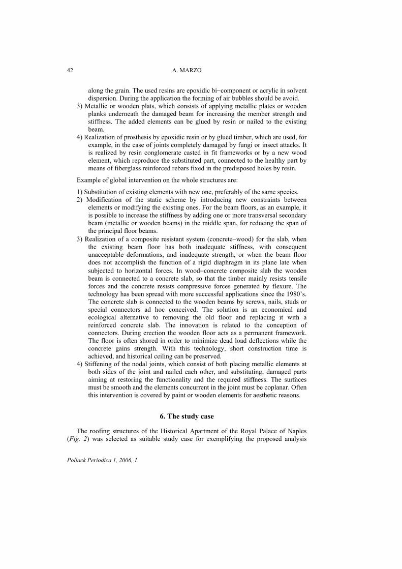
42 A. MARZO
along the grain. The used resins are epoxidic bi−component or acrylic in solvent dispersion. During the application the forming of air bubbles should be avoid.
3) Metallic or wooden plats, which consists of applying metallic plates or wooden planks underneath the damaged beam for increasing the member strength and stiffness. The added elements can be glued by resin or nailed to the existing beam.
4) Realization of prosthesis by epoxidic resin or by glued timber, which are used, for example, in the case of joints completely damaged by fungi or insect attacks. It is realized by resin conglomerate casted in fit frameworks or by a new wood element, which reproduce the substituted part, connected to the healthy part by means of fiberglass reinforced rebars fixed in the predisposed holes by resin.
Example of global intervention on the whole structures are:
1) Substitution of existing elements with new one, preferably of the same species. 2) Modification of the static scheme by introducing new constraints between
elements or modifying the existing ones. For the beam floors, as an example, it is possible to increase the stiffness by adding one or more transversal secondary beam (metallic or wooden beams) in the middle span, for reducing the span of the principal floor beams.
3) Realization of a composite resistant system (concrete−wood) for the slab, when the existing beam floor has both inadequate stiffness, with consequent unacceptable deformations, and inadequate strength, or when the beam floor does not accomplish the function of a rigid diaphragm in its plane late when subjected to horizontal forces. In wood−concrete composite slab the wooden beam is connected to a concrete slab, so that the timber mainly resists tensile forces and the concrete resists compressive forces generated by flexure. The technology has been spread with more successful applications since the 1980’s. The concrete slab is connected to the wooden beams by screws, nails, studs or special connectors ad hoc conceived. The solution is an economical and ecological alternative to removing the old floor and replacing it with a reinforced concrete slab. The innovation is related to the conception of connectors. During erection the wooden floor acts as a permanent framework. The floor is often shored in order to minimize dead load deflections while the concrete gains strength. With this technology, short construction time is achieved, and historical ceiling can be preserved.
4) Stiffening of the nodal joints, which consist of both placing metallic elements at both sides of the joint and nailed each other, and substituting, damaged parts aiming at restoring the functionality and the required stiffness. The surfaces must be smooth and the elements concurrent in the joint must be coplanar. Often this intervention is covered by paint or wooden elements for aesthetic reasons.
6. The study case
The roofing structures of the Historical Apartment of the Royal Palace of Naples (Fig. 2) was selected as suitable study case for exemplifying the proposed analysis
Pollack Periodica 1, 2006, 1

METHODOLOGY FOR STRUCTURAL ANALYSIS OF WOODEN STRUCTURES 43
methodology for historical complex wooden structures. The structures under study, datable about the XVIII century, are composed by two different substructures, which are typical of the constructional practice of that time in important buildings: the vault and the beam floor connected each other.
HONOUR CORT
PENSILE GARDENPL
EBIS
CIT
O S
QU
AR
E
Fig. 2. a) Bird’s eye view; b) Historical Apartment of the Royal Palace of Naples
In particular a wooden vault was usually erected as false ceiling, at the intrados of which an internal coat of thin canes and a cover of stucco provided the base of the paint. The examined vaults are realized in three different geometrical configurations. In the first one the vault is self−bearing, in fact it leans on the perimeter masonry walls only (Fig. 3a); in the second one the vault is partially suspended to the upper floor (Fig. 3b); in the third one the vault is suspended to an above structure independent from the floor (Fig. 3c), composed by beams with a rectangular cross section.
beam floor
vault supporting structure vault link
b) a)
beam floor
vault
link
vault
b)a) c)
Fig. 3. Typologies of vault supports: a) self−bearing vault; b) vault partially suspended to the floor; c) vault independents to the floor
The connections among structural elements are realized by means of iron nails with a rectangular cross section. The detailed geometric and mechanical in−depth surveys have been carried out, aiming at identifying the wooden species, the geometrical configuration of the structures, the element shapes, the defects and any damages due to the overstress and/or the insect or fungi attacks. The mechanical properties of the used materials have been measured by experimental tests in laboratory and in situ investigations.
Pollack Periodica 1, 2006, 1

44 A. MARZO
On the basis of the acquired knowledge, for each structure a three−dimensional FEM model, has been set−up by using the program of structural calculus Sap2000 [4], in order to evaluate the capacity in terms of resistance and deformation performs. The analysis of the structural behavior evidences the weaknesses of the structure in terms of resistance and deformation capacities. The safety checks have been performed and the restoration interventions, conceived for upgrading and retrofitting the wooden structure, have been proposed, according to the analysis results.
6.1. In situ investigations
Aims of the in situ investigations were the identification of the species, the measurement of the moisture content, the survey of any defects and the degradation state due to aging, to fungi attacks, further to the joints effectiveness. They were carried out according to the Italian current standard rules (UNI 11118 and UNI 11119). After an in depth visual investigations several ND tests were executed. The moisture content was measured by means of hygrometer for wood. The measurements were carried out for each structural element near both supports, which are critical parts when they are in contact with masonries, and for at least three sections along the span. The identification of the species was performed by means of taking out from the beams of little core, whose diameter was about 5 mm and the length about 70 mm. Those specimens were analyzed by microscope to establish the species and the age of the beam, which they belong to. The presence of defects and the degradation state were surveyed through an in−depth visual investigation with the help of simple tools, as screwdriver, rubber hammer, and resistographic tests. The results of the investigation are the distribution of fungi and insect attacks for each beam, and the map of the defects (knots, shakes, creaks), which are used for the ancient wooden elements grading.
6.2. The material mechanical properties
According to the constructional practice of the XVII and XVIII centuries, the wooden beam floors and their stiffening systems are made of chestnut, whereas the wooden structure of the vault is made of poplar, which is lighter. For the new wood of chestnut and poplar, the technical literature [2], [5] specifies the values for the density (γ) and the elastic modulus in the longitudinal direction (E0), as indicated in Table I. The elastic modulus in the transverse direction (E90) can be calculated with good approximation considering that for the hardwood species it is equal to about 4.8 % of E0. The tangent modulus G, which is expressed by the ratio E/2(1+ν), is calculated according to different values of the Poisson coefficient ν in the longitudinal direction ν0 and in the transverse direction ν90. In the case of ancient wood, considering that it could be affected by defects and degradations, together with working lacks, such as shape irregularity of structural members, non planarity of the sub−structure, connection inaccuracy, the consequent stiffness reduction of the structural members is considered by assuming the mean value of the longitudinal elastic modulus, obtained by means of laboratory bending tests on chestnut wood beams, having the same age of the structure under study [6], [7]: E0,e,m= 8900 kN/m2×10-3. This value corresponds to a reduction as respect to the new
Pollack Periodica 1, 2006, 1

METHODOLOGY FOR STRUCTURAL ANALYSIS OF WOODEN STRUCTURES 45
wood of about 25 %. This reduction allows taking account of the ancient wood degradation due to aging, during the implementation of the FEM Model, since it is set up without defects (Table I).
Table I
Mechanical properties of the wood
Species γ E0 E90 ν0 ν90 G0 G90 kN/m3 kN/m2×10-3 kN/m2×10-3
Nominal mechanical properties of the new wood Chestnut 5.80 11380 544 0.37 0.46 4153 185 Poplar 3.40 7850 376 0.38 0.47 2844 128
Predicted mechanical properties of the ancient wood Chestnut 8535 408 3115 139 Poplar 5887 282 2133 96
Concerning the metallic elements, the iron with a tensile strength equal to 320 MPa is assumed, according to the strength properties of the material used at the time of the structure erection [8].
6.3. The geometrical model
Due to the high level of variability and irregularity, which is peculiar of the ancient wooden structures, the geometrical modeling is necessarily affected by some approximation, which is due to the variability and irregularity of the element shapes and connection types. The approximations are always made on the safe side. This simplifies the structural rendering preserving the actual mutual contribution of each sub−structure to the overall behavior of the structural complex. A 3D model of the structure is implemented by using the program of structural calculation SAP2000 vers.7.12 [4].
7. The Diplomatic Hall
As an example the attention is focused on one of the study halls: the Diplomatic Hall. The geometric and mechanical surveys, together with the modeling aspects and the results of the structural analysis were presented [9], together with the proposed retrofitting intervention [10].
7.1. The geometrical survey
The Diplomatic Hall is the II hall in the Fig. 2b, which complex wooden structure is composed by three main sub−structures:
1) the vault; 2) the beam floor; 3) the truss.
Pollack Periodica 1, 2006, 1

46 A. MARZO
The vault (Fig. 4a) is made of wooden grid elements, ribs and splines, shaped as a reversal boat keel. Ribs simply abut to the perimeter masonry walls, whereas they are nailed at the ends at the vault crown. Splines are orthogonal to ribs and fixed to them by a half−lap joint. The horizontal part at the vault crown is realized by a rectangular grid of wooden elements with circular section, which are nailed each other at the intersection point and enclosed in a perimeter rectangle, whose elements are nailed each other and to the vault ribs. At the intrados of the vault a coat of thin canes, lime and plaster, as an overlay of the wooden structure, and the cover of stucco, as the base of the fresco, were realized. The vault is partially suspended to the floor above, in fact it is both leaned on the perimeter masonry walls and connected to the floor by means of wooden links. It realizes the false ceiling.
Fig. 4. a) Vault carpentry; b) Beam floor carpentry; c) Sections A−A; d) Section B−B; e) Truss
The primary frame of the beam floor (Fig. 4b) is arranged along the minor span. Each beam is composed by two wood stocks placed side by side at the mid−span, connected each other by nails. The floor beam is stiffened by means of three different systems:
1) a system of three series of four transversal inclined struts arranged in planes perpendicular to the primary beam axes (Fig. 4c);
Pollack Periodica 1, 2006, 1

METHODOLOGY FOR STRUCTURAL ANALYSIS OF WOODEN STRUCTURES 47
2) two transversal secondary beams, orthogonal to the primary beams (Fig. 4d); 3) longitudinal secondary beams set under the primary beams, parallel to them and
connected to longitudinal inclined struts, forming a supporting portal frame, which the wooden links of the vault are connected to; they are placed at all beams, with the exception of three alignments of beams near the perimeter masonries (Fig. 4d).
The floor slab is composed by planks with a semi−circular cross section, over which a lapilli layer and cement lime mortar is cast. By in situ measurements, the layer thickness varies from about 10 cm at the support to masonry to 40 cm in the middle span. The truss (Fig. 4e) is close to the middle span of the floor slab, orthogonal to the primary floor beams. It is 7.00m heights. Its struts are composed by different wood stock parts, placed side by side and nailed each other, with a variable cross section along the element axis. The tie beam has a circular cross section, it is connected to some floor beams by means of metallic U shaped stirrups. In view of the retrofitting intervention, the vault has been propped up by provisional supports.
7.2. The structural model
A 3D model of the structure was implemented for using in the program of structural calculation SAP2000 [4]. The modeling assumptions are specified in Mazzolani et al., 2004 [9]. Fig. 5 shows the extruded model at the truss beam location in both XZ and YZ planes and the vault model.
Fig. 5. Extruded structural models
7.3. The load analysis
Load combinations were applied for the Ultimate and the Serviceability Limit States safety checks, according to EUROCODE 5. Concerning the load analysis, for the vault, the dead load is due to the contribution of the lathing, the stucco and the plaster, corresponding to 1 kN/m2, which is applied as a distribution of forces concentrated at the grid nodes. The values of dead load and live load applied on the floor are Gk=7.0 kN/m2 and Qk=2.0 kN/m2, respectively, considering that the above rooms are for residential use. Different load conditions, which the structure is supposed to have undergone, starting from the successive erection stages until the service load condition, were analyzed, in order to go along the stress and strain states during the service life of the complex structure from the beginning until today. In particular the following phases and corresponding structural models have been identified [9]:
Pollack Periodica 1, 2006, 1

48 A. MARZO
1) erection of the floor structure (Model 1); 2) erection of the truss (Model 2); 3) erection of the vault (Model 3); 4) floor structure completion (Model 4); 5) connection vault−floor beam and vault completion (Model 5); 6) service conditions (Model 6).
7.4. Evaluation of the deflection state
For estimating the overall deflection, deriving from the complete erection of the wooden structure, the material is modeled as new wood, this assumption being reasonable at the time of the original erection. According to EC5, three effects were considered, aiming at evaluating the actual deflection state of the whole wooden structure, for the worst climatic condition:
1) the reduction of the elastic modulus to consider the typical degradation of ancient wood;
2) the creep, such as the material strain at constant load; 3) the moisture content of material.
As reference parameters, vertical displacements (uz) of the floor beam midsections are assumed. With regards to the floor beams, the results of the analyses show that beam deflections are below the safety limits when new wood is considered. On the contrary, the degradations and the time dependent effects of creep and moisture contents induce an increase of deflections, which for the beams is beyond the limits (umax= 0.09 m). In particular for the beams did not connect to the tie beam of the truss the increase is about 0.05 m, while for the other ones is about 0.03 m. Therefore the beneficial effect of the truss induces a displacement reduction of about 50 % in the connected floor beams. With regards to the vault, the deformation state, which determines the crack distribution requiring the restoration intervention of the fresco, was evaluated, considering the effect of degradation due to ancient wood, creep and moisture. The vault undergoes a flattening, which consists of sagging at the center, with a maximum displacement equal to 9 cm, and elevation near the masonry supports, with a maximum displacement equal to 1.54 cm. In Fig. 6 together with the crack distribution, the model at a typical structural section, the bending moment distribution and the corresponding deformed configuration are drawn.
7.5. Evaluation of the stress state
Aiming at the strength and stability checks, the influence on the material strength of the load application duration and of the wood moisture was accounted for according to EC5, by a reduction factor, which has been assumed as equal to about 0.5 [10]. Thus, the design strength listed in Table II for the relevant stress conditions and wood species were used. Results emphasized that some ribs of the vault do not accomplish the strength requirements and all the struts of the floor beam stiffening systems do not satisfy the stability checks.
Pollack Periodica 1, 2006, 1

METHODOLOGY FOR STRUCTURAL ANALYSIS OF WOODEN STRUCTURES 49
Fig. 6. a) Crack distribution at the vault intrados; b) the model at a typical structural section; c) the bending moment distribution
7.6. The proposed intervention
The proposed retrofitting intervention is based on the use of the so called mixed technologies, consisting in the combination of techniques, which use different materials (in the specific case new wood, steel, reinforced concrete, rubber) for realizing local strengthening systems of the existent structures [10]. The prerogatives of such retrofitting technologies are the reversibility, the lightness, the ductility, and the easiness of material supply, transportation and erection. Different retrofitting techniques are conceived according to the needs of each simple substructure.
Table II
Design strength fd (kN/m2×10-3)
Wood species Stress condition Chestnut Poplar Compression // to the grain (fc,0,d) 13.0 10.0 Tension // to the grain (ft,0,d) 12.0 6.5 Bending (fm,d) 20.0 11.0 Shear (fv,d) 1.9 1.2
For the beam floor the retrofitting interventions consists of the following systems:
a) the casting of a reinforced lightened concrete slab, which collaborates with the floor beams by means of a system of steel connectors purposely conceived with an “ad hoc” shape;
b) the reinforcement of the unstable longitudinal struts and transverse radial struts, by means of both horizontal and vertical stiffening elements.
For the vault, the retrofitting intervention involves the vault−floor links only. In fact, from the examination of the internal actions’ distribution within the vault structural
Pollack Periodica 1, 2006, 1

50 A. MARZO
members, it appears that links between vault and floor beams located near the masonry supports are harmful, they working as struts, exerting an additional bending action within the ribs. The removal of all these links placed at the vault−curved sides induces a strong reduction of the internal actions. As a consequence, the retrofitting intervention consists in the removal of all the wooden links, replacing them only at the horizontal vault crown by means of steel ties. The r.c. slab is 20 cm thick, it is lightened by polystyrene blocks, 10 cm high (Fig. 8). The slab is reinforced by a net of steel rebars, 6 cm diameter and 20 cm mesh, disposed at the extrados. The concrete slab is cast on fir planks, 3 cm thick, which function as fix formworks. The wooden planks should be protected from the water of the cast by a plastic film and in any case the water content of the concrete should be limited. Wooden beams – r.c. slab connectors are realized by sleeves made of cold−formed steel, which are composed by four parts, whose shape depends on the transversal section. The type A is used for single sections, the type B is used for double sections and the type C is used for triple sections. The three different types of sleeve are shown in Fig. 7. They have perpendicular drilled wings connected each other by means of bolted connections. The vertical superior wings serve as connectors and they are immersed in the concrete cast, guaranteeing the transmission of the sliding actions. Therefore, steel sleeves have a twofold function:
1) they exert a transversal ringing action on the beams; 2) they realize the beam−concrete slab connection without the need to drill the
beams.
In particular, such connectors do not weaken the cross section and produce a beneficial effect of confinement. Due to the variability of the beams cross section, in order to avoid the use of many sleeve geometries, the connection system is obtained by adapting to the actual beam cross−section a rubber layer, which is vulcanized to the steel sleeves. In this way three different types of connection elements are used only. The in plane layout of the connection elements is plotted in Fig. 8a.
50
1010 3
polyst. blocksteel sleeve
r.c. slab
plancks
rubber polyst. block rubber
r.c. slab
plancks
steel sleeve
1010 3
polyst. block
r.c. slab
plancks
steel sleeverubber
1010 3
b) c)a)
Fig. 7. Types of connection elements: a) type A; b) type B; c) type C
In correspondence of the vault crown the vault−floor connection is realized by a steel plate vertical tie, bolted at both ends (Fig. 8b): above, to the connection elements, and below to the steel sleeve, which is located astride to an element of the horizontal grid of the vault crown. In correspondence of the longitudinal and transversal struts a
Pollack Periodica 1, 2006, 1

METHODOLOGY FOR STRUCTURAL ANALYSIS OF WOODEN STRUCTURES 51
steel pipe is bolted at both ends: above, to the connection elements, and below, to the steel sleeve, which is located astride to an element of the struts, in order to stiffen the struts in the vertical plane (Fig. 8b and c). Furthermore, tubular horizontal steel profiles connect the vertical steel pipes each other and to the perimeter masonries, in order to stiffen struts in the horizontal plane (Fig. 8c).
steel pipes
r.c. slabvault-beam floor connection connection element
steel plate
connection element
steel sleeve14
.20
16.60
connection element wooden beam
polystyrene blocksteel pipe connection element
r.c. slab
stiffening systemstubular steel profile
b)
a) c)
Fig. 8. Location of stiffening system: a) Plan layout; b) Longitudinal section; c) Transversal section
8. Conclusion
The paper deals with a methodology for the analysis of complex historical wooden structures. The study of the historical wooden structures is also made difficult by the little information related to their technology of realization and their inaccessibility to carry out in depth surveys or investigations. Therefore the set up of numerical models for analyzing the behavior of ancient wooden structures is affected by any approximations, which have to be made in the safe side. An overview of the Italian and the European existing roles has been introduced, emphasizing the lack of regulations about ancient structures. Moreover a procedure for restoration intervention of historical wooden structures has been discussed, in addition of some of most common retrofitting interventions, highlighting that the main prerogatives of the retrofitting systems are the reversibility of the technology, the lightness, the ductility, the easiness of supply, transportation and erection. At the end, an appropriate analysis methodology was applied to a study case. With reference to the roofing structures of the Diplomatic Hall of the Royal Palace of Naples (Italy) the geometric and mechanical surveys, together with the modeling aspects and the results of the structural analysis were presented. The analysis of the structural behavior evidences the weaknesses of the structure in terms of resistance and deformation capacities. Consequently to the safety checks, a restoration intervention has been proposed for upgrading and retrofitting the wooden structure. It is based on the use
Pollack Periodica 1, 2006, 1

52 A. MARZO
of the so−called mixed technologies, consisting in the combination of techniques, which use different materials (in the specific case new wood, steel, reinforced concrete, rubber) for realizing local strengthening and stiffening systems of the existent structures. The same methodology has been applied to other Halls of the Historical Apartment, whose analyses are still in progress.
Acknowledgement
The author would like to acknowledge Prof. Federico M. Mazzolani for his invaluable guidance during her research activity and Eng. Beatrice Faggiano for her constant assistance.
References
[1] CEN (European Communities for Standardisation), Final draft prEN 1995−1−1 2002. Eurocode 5: Design of timber structures − Part 1−1: General rules − General rules and rules for buildings.
[2] Giordano G. Tecnica delle Costruzioni in legno (Wooden structure engineering), HOEPLI ed., Milan, Italy, 1989.
[3] Forest Products Laboratory, Wood Handbook − Wood as an engineering material, U.S. Department of Agriculture, Forest Service, March 1999.
[4] Wilson E.L. Three dimensional static and dynamic analysis of structures, Berkeley, California, USA, Computers & Structures Inc., 1998.
[5] Uzielli L., Bonamini G., Noferi M., Togni M. Il manuale del legno strutturale vol.1 – Ispezione e diagnosi in opera (Manual of the structural wood– Inspection and diagnosis in situ), Mancosu ed., Rome, Italy, Vol. 1, 2001.
[6] Calderoni B., De Matteis G., Mazzolani F.M. Structural performance of ancient wooden beams: experimental analysis, European timber buildings as an expression of technological and technical cultures, Editions Scientifique et Medicales, Elsevier S.A.S., 2002, pp. 217−233.
[7] Mazzolani F.M., Calderoni B., De Matteis G., Giubileo C. Experimental analysis of ancient wooden beams for flexural and shear failure. Proc. of the 4th International Seminar “Structural analysis of historical constructions”, Padova, Italy, 10−13 November Vol. 1, 2004, pp. 903−910.
[8] Breymann G.A. Trattato generale di costruzioni civili con cenni speciali alle costruzioni grandiose (General treaty about civil constructions with outline about magnific ones, 5 Vol., in III Vol. Costruzioni metalliche (Costruzioni in ferro) (Metallic structures), Vallardi ed., Milan, Italy 1889.
[9] Mazzolani F.M., Faggiano B., Marzo A. Methodology for the analysis of complex historical wooden structures: a study case. Proc. of the IV International Seminar “Structural Analysis of Historical Constructions (SAHC)”, Padova, Italy, 10−13 November Vol. 2, 2004, pp. 945−955.
[10] Mazzolani F.M., Faggiano B., Marzo A. Retrofitting of complex wooden structures by means of mixed reversible technologies: a study case. Proc. of “COST C12” Final conference, Innsbruck, Austria, 19−22. January 2005, pp. 587−597.
Pollack Periodica 1, 2006, 1

POLLACK PERIODICA An International Journal for Engineering and Information Sciences
DOI: 10.1556/Pollack.1.2006.1.4 Vol. 1, No. 1, pp. 53–66, (2006)
www.akademiai.com
EXPERIENCES ON HYDRAULIC PERFORMANCE OF SUB−SURFACE FLOW CONSTRUCTED
WETLANDS
Erno DITTRICH
Department of Environmental Engineering, Pollack Mihály Faculty of Engineering, University of Pécs, Boszorkány u. 2, H−7624 Pécs, Hungary, e−mail: [email protected]
Received 2 January 2006; accepted 10 April 2006
Abstract: In this article new result of international researches focused on the hydraulic behavior of the subsurface−flow constructed wetlands (SF−CW−s) for wastewater treatment are shown. The results presented below are focused on the tracer experiments to simulate transport processes, the effect of Total Suspended Solids (TSS) and organic substances loads, and the effect of macrophytes, meteorological conditions. The Hungarian experiences of constructed wetlands are compared to that of international ones and the main differences are discussed. The main considerations of comparison are: specific load of organic substances, specific load of TSS, specific hydraulic load, the type of soil, the pre−treatment systems, etc. The conclusion of this comparison is the main directions of development of the subsurface−flow constructed wetlands in Hungary. Keywords: Subsurface−flow constructed wetlands, Hydraulic transport and mixing, Clogging, TSS load, Load of organic substances, Macrophytes
1. Introduction
Designing, constructing and operating of wastewater treatment plants is one of the important parts of civil engineering practice and significant part of environmental protection, too. So, lot of engineers and scientists are interested in development and research of wastewater systems. Today, a range of different wastewater treatment systems is available. These can be classified as follows:
a) Intensive technologies such as activated sludge systems, trickling filters, Sequencing Batch Reactors (SBR), etc;
HU ISSN 1788−1994 © 2006 Akadémiai Kiadó, Budapest

54 E. DITTRICH
b) Extensive technologies such as ponds, constructed wetlands (CW−s), irrigation systems, etc.
Simple construction, large buffering capacity, little excess sludge production, simple operation and maintenance, low operational and maintenance costs are the main advantages of extensive systems [1]. CW−s are used as wastewater treatment systems from the 70’s, when Kickuth (1977) published his root−zone method. CW−s as wastewater treatment systems are very popular in West−Europe, USA and Australia and are getting popular worldwide. Two main different type, can be designed within CW−s:
a) Free−surface flow systems (FS−CW−s); b) Sub−surface flow systems (SF−CW−s).
In FS−CW the wastewater flows through the system with free surface. In the SF−CW−s – usually pre−treated – the wastewater flows through the filter media is planted with macrophytes (f.e. Phragmatis australis). The first Hungarian SF−CW was constructed in Tóalmás in 1991 [2]. Now there are 16 SF−CW−s in Hungary. There are 10 domestic wastewater treatment plants (Boldog, Kacorlak, Kám, Salgótarján, Sióagárd, Szépalmapuszta, Szügy, Tóalmás, Fertőrákos, Komlódtótfalu) and 3 septic−tank disposal treatment plants (Aparhant, Magyarbóly, Bakonyszombathely) and 2 industrial wastewater treatment plants (Kerecsend, Demjén). There is an agricultural wastewater treatment plant in Hódmezővásárhely. The Hungarian experiences of operational SF−CW−s are more unfavorable than the West−European ones. This is one of the reasons why SF−CW as wastewater treatment technology type is not too popular. This article will show that is mainly owing to inadequacies of the Hungarian designing practice. The aim of this article to show the new results of international researches focused on the hydraulic behavior and on the problems of numerical hydraulic modeling of the subsurface−flow constructed wetlands (SF−CW−s) for wastewater treatment. This article will make a comparison between the Hungarian and the international experiences. The conclusion will be the main directions of development of the subsurface−flow constructed wetlands in Hungary.
2. Main construction types
There are two main construction types of SF−CW−s:
a) Vertical flow systems (Fig. 1); b) Horizontal flow systems (Fig. 2).
The main differences between these two types are the main flow direction, the contact time, the mode of oxygen transport, and the saturation in the volume of substrate.
Pollack Periodica 1, 2006, 1

EXPERIENCES ON SUB−SURFACE FLOW CONSTRUCTED WETLANDS 55
3. Ideal flow distribution in SF−CW−s
3.1. Ideal flow distribution in horizontal flow systems
Let us suppose that the filter media has the same condition in time and in it’s volume, and the flow−system is permanent saturated flow. The most simple equation expressing the flow regime in horizontal flow systems is Darcys’ law [3]:
, (1) )( hkgradv ⋅−=
where v is the pore−water velocity [m/d], k is the hydraulic conductivity of media [m/d], h is the the level of pressure potential [m]. If it is supposed that the flow−regime is one−dimensional and the bottom slope is constant, we can get the simple form of Darcy’s law:
, or Skv ⋅= SkAQ c ⋅⋅= , (2)
where S is the bottom slope [m/m], Q is the hydraulic loading rate [m3/d], Ac is the cross sectional area [m2].
Fig.1. Cross section of vertical flow system
Fig.2. Horizontal flow system
Pollack Periodica 1, 2006, 1

56 E. DITTRICH
The flow regime can be described 2 or 3 dimensionally with Boussinesq’s equation. This is the 2D−form of Boussinesq’s equation below [4]
t
xthkn
xx
xtzxth
∂∂
⋅=∂
∂∂
⋅∂ ),(),(),(
, (3)
where n is the porosity of the media [−], z is the distance between the water level and the fixed relative level [m], x is the horizontal coordinate [m], t is the time [d]. It has to be supposed that the distribution of flow is uniform along the distribution pipe at 2D describing mode. The hydraulic processes can be modeled more precise with this equation as non−permanent, saturated flow. The main problem is that a huge amount of data is needed to calibrate the hydraulic−model. If data enough are available it could be solved to take changes of porosity and hydraulic conductivity in consideration in the hydraulic model.
3.2. Ideal flow distribution in vertical flow systems
There is unsaturated non−permanent flow in these types of systems with vertical flow direction. Let us suppose that the filter media has the same condition in time and in volume, and the flow−distribution is uniform along the distribution pipe−system. So the flow−regime can be described 2 or 3 dimensionally with Richard’s equation [5, 6]
⎟⎠⎞
⎜⎝⎛
∂+∂
⋅⋅∂∂
−⎟⎠⎞
⎜⎝⎛
∂∂
⋅⋅∂∂
−==∂
∂⋅
zzk
zxk
xdtd
tc ψψψψΘψψ )()()( , (4)
where Θ is the volumetric water content of the media [−], ψ is the matrix potential [m]. The main problems are that a huge amount of data is needed to calibrate the hydraulic−model, and dynamical changes of the water content in the pore−system.
3.3. Ideal transport processes in SF−CW−s
By injecting a tracer into the system, an assessment of the hydraulic regime can be obtained. After the injection the residence time distribution (RTD) can be measured at the outflow. The real average hydraulic retention time (HRT) can be calculated from RTD−function. The difference between the real HRT distribution and the theoretical HRT shows the degree of hydraulic irregularities. The simplest method to design the hydraulics of SF−CW−s is the supposition of plug−flow in the construction. Than the theoretical HRT can be calculated as
QVnHRT ⋅
= , (5)
where V is the effective volume of substrate [m3]. The plug−flow design assumption does not describe adequately the water flow through the SF−CW [7]. The transport process of conservative tracer is composed of
Pollack Periodica 1, 2006, 1

EXPERIENCES ON SUB−SURFACE FLOW CONSTRUCTED WETLANDS 57
advection and dispersion. The 1D transport equation to conservative tracer in porous media is [8]
xC
Rv
xC
Rv
tC xxL
∂∂
−∂∂
⋅⋅
=∂∂
22α
, (6)
xxT Dv =⋅α , (7)
where Dx is the dispersion constant [m2/d], vx=Q/Ac is the average pore−water velocity [m/d], Lα is the dispersion coefficient [m], R is the retardation coefficient [−], C is the tracer concentration [g/m3], x is the longitudinal coordinate [m], t is the time [d]. From this viewpoint the application of R is different from the conventional interpretation. In this solution R is applied to describe the dead−zones of flow regime. So in this case R>1, and it can be calculated from the rate of dead−zones in the construction
hVV
VR−
= . (8)
The momentum of conservative tracer injection can be described with the Dirac−delta function at x=0 and t=0
)()0,( xRwmn
MxC δδ ⋅⋅⋅⋅
= , (9)
where M is the mass of tracer [kg], m is the average depth of water level [m], w is the infinitesimally small width of the flow−system [m]. If C(±∞,t)=0, the analytical solution of the 1D transport equation (6) is [8]
⎥⎥⎥⎥⎥
⎦
⎤
⎢⎢⎢⎢⎢
⎣
⎡
⋅⋅
⎟⎠
⎞⎜⎝
⎛ ⋅−
−⋅⋅⋅
⋅⋅⋅⋅⋅
=
Rtv
Rtvx
Rtv
Rnmw
MtxCxL
x
xLα
απ4
exp
2
),(
2
0
. (10)
This solution is the Gauss−distribution curve. This curve flows with vx/R average velocity, and the function of spreading is
RtvxL /2 ⋅⋅= ασ . (11)
It is easy to describe the transport of conservative tracer with these equations, if the significant parameters are known. The solution is illustrated in Fig. 3. The RTD−curve can be calculated from Eq. (10) at the measurement point, if x=L [m] the distance from the injection point is known. The form of RTD−curve by way of ideal transport processes (dispersion and advection) is illustrated in Fig. 4.
Pollack Periodica 1, 2006, 1

58 E. DITTRICH
4. Real flow distribution in SF−CW−s, international experiences
4.1. Main differences between ideal and real flow distribution
There are significant differences between ideal and real flow distribution. The main reasons of these differences are:
a) the impacts of the weather: rainfall, evapotranspiration, freezing, snow melting; b) deficiencies of the construction: differences of hydraulic conductivity and
porosity of the filter media, deficiencies of distribution pipe−system; c) clogging processes: deposition of organic and inorganic particles, microbial
biomass (bio−film activity), root−growing in the filter−media, mechanical compaction of the media, chemical precipitation and deposition in media, entrapped gas blocking the pores.
The measures of these effects to the real flow distribution, have been collected in Table I from the international specified literature. A goal of recent research is to develope a numerical hydraulic modell, that can able to simulate the real flow distribution. This model is based on the equations have been presented in Paragraph 2. The CW is modelised as a few Completely Stirred Tank Reaktors (CSTR) in series. The number of these reactors debend on the measure of the effects are shown in Table I. In this hydraulic modell it does not need to take in consideration the insignificant factors from the incelement effects (Table I). In spite of the fact the number of remainder factors are numerous, so the model calibration should be done step by step. The effects of factors should be separated at the data collection step because of the complex effects in the examined construction. This separation form a very interesting goup of problem. The number of seasonally significant factors (group of weather factors) can be reduced by chosen of good weather period (f.e. chosen of dry and warm periods). The group of construction factors has to be measured before the clogging processes had started in the construction. The factors of clogging group are depending on the temperature, seasonality, hydraulic loading rate, TSS loading rate, organic−substances loading rate, etc. So, it needs to make a precise and komplex monitoring to separate the effects of these factors. The best method to separate these effects to measure tracer response curves step by step in the agequate “moments” in the lifetime of examined CW−s.
C
x
t=0
t=t1
t=t2t=t3 t=t4
Fig.3. The transport of conservative tracer in porous media suggested plug flow
with dispersion of [7]
Pollack Periodica 1, 2006, 1

EXPERIENCES ON SUB−SURFACE FLOW CONSTRUCTED WETLANDS 59
C
t
Fig. 4. The calculated RTD curve from the 1D transport equation
Table I
The measure of the effects to the flow distribution
Vertical flow system Horizontal flow system Group of factors Factors Measure of
effect Ref. Measure of effect Ref.
rainfall seasonally sign. [7, 18] seasonally
sign. [7, 15, 18]
evapotraspiration seasonally sign. [7, 18] seasonally
sign. [7, 9, 18]
dissolution of snow
seasonally significant − seasonally
sign. − whe
athe
r
freezing insignificant − insignificant − diff. of hydr. cond. and porosity significant − significant [10]
deficiencies of distr. pipe system significant − significant [19]
cons
truct
ion
shape of media volume significant [14] significant [14]
depositioning of particles significant [12, 14] significant
microbial biomass significant [6, 12] significant root density insignificant [12] significant mechanical compction insignificant [12, 13] insignificant
chemical precipitation insignificant [12, 13] insignificant
clog
ging
gas blocking insignificant [12, 13] insignificant
As a result of these factors (Table I) there are incelement effects to the opreation of the constructions:
a) inclement effects to the hydraulic behaviour: chanelling [9, 10], short−circuiting [9, 10], surface−flows [11], ponding [12, 13];
b) inclement effects to the transport processes: irregular mixing processes [14], lower detention time than the theoretical value [9, 15, 16];
Pollack Periodica 1, 2006, 1
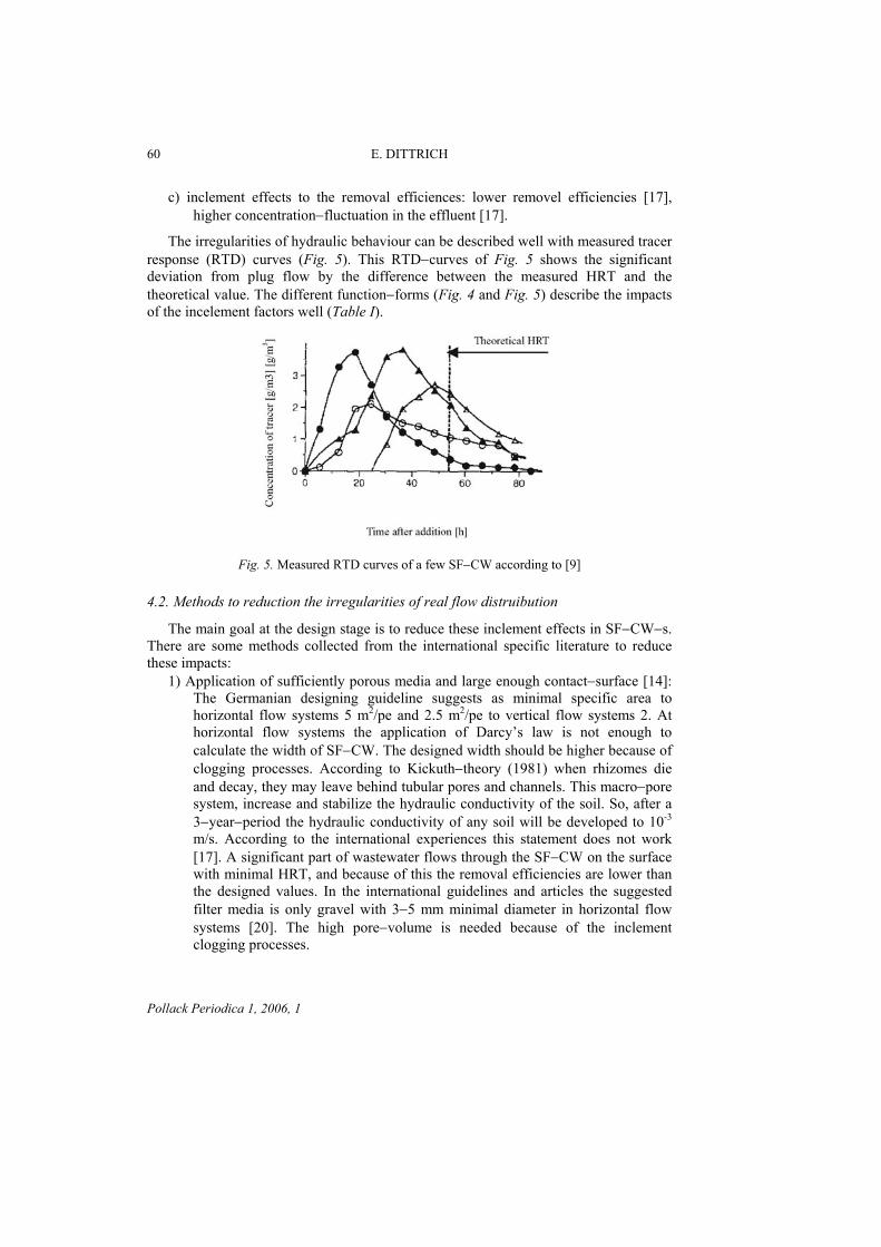
60 E. DITTRICH
c) inclement effects to the removal efficiences: lower removel efficiencies [17], higher concentration−fluctuation in the effluent [17].
The irregularities of hydraulic behaviour can be described well with measured tracer response (RTD) curves (Fig. 5). This RTD−curves of Fig. 5 shows the significant deviation from plug flow by the difference between the measured HRT and the theoretical value. The different function−forms (Fig. 4 and Fig. 5) describe the impacts of the incelement factors well (Table I).
Fig. 5. Measured RTD curves of a few SF−CW according to [9]
4.2. Methods to reduction the irregularities of real flow distruibution
The main goal at the design stage is to reduce these inclement effects in SF−CW−s. There are some methods collected from the international specific literature to reduce these impacts:
1) Application of sufficiently porous media and large enough contact−surface [14]: The Germanian designing guideline suggests as minimal specific area to horizontal flow systems 5 m2/pe and 2.5 m2/pe to vertical flow systems 2. At horizontal flow systems the application of Darcy’s law is not enough to calculate the width of SF−CW. The designed width should be higher because of clogging processes. According to Kickuth−theory (1981) when rhizomes die and decay, they may leave behind tubular pores and channels. This macro−pore system, increase and stabilize the hydraulic conductivity of the soil. So, after a 3−year−period the hydraulic conductivity of any soil will be developed to 10-3 m/s. According to the international experiences this statement does not work [17]. A significant part of wastewater flows through the SF−CW on the surface with minimal HRT, and because of this the removal efficiencies are lower than the designed values. In the international guidelines and articles the suggested filter media is only gravel with 3−5 mm minimal diameter in horizontal flow systems [20]. The high pore−volume is needed because of the inclement clogging processes.
Pollack Periodica 1, 2006, 1

EXPERIENCES ON SUB−SURFACE FLOW CONSTRUCTED WETLANDS 61
2) In the vertical flow systems gravel should not be used as filter media because of the too short HRT. So the researchers usually suggest sand or sandy−gravel layer with 60 cm depth as filter media with garvel size of 0.06−4 mm. More criterias to filter media are d10>0.2 mm and U=d60/d10<5 [21, 22].
3) Application pretreatment systems with high TSS removal efficient: The TSS−loading is one of the main reasons of clogging processes, so it has to be limited. The suggested maximum values are different in the literature: 5 g/m2,d [13], 7 g/m2,d [20].
4) Limitation of the organic substances loading: The organic substances loading is the other main reason of clogging processes, so it has to be limited too. The suggested maximum values from the literature are different: 20 gCOD/m2,d [13], 25 gCOD/m2,d [23], (COD: Chemical Oxigen Demand).
5) Resting beds periodically: The clogging process is partly reversible. In order to prevent the system from long term clogging, it is useful to have at least 2 or more beds in parallel, and operation periodically [12, 13].
6) Accurate placement of media and distribution−pipe system to get uniform media porosity and flow distribution [10].
7) Placement the surface of media with minimal back−slope: It is needed to reduce the decrease of HRT caused by surface flows.
8) Limitation of hydraulic loading rate (HLR). The maximum value of HLR should not exceed 40 mm/d at horizontal flow systems, and 60 mm/d at vertical flow systems [22, 24].
5. Analysis of Hungarian SF−CW−s
5.1. Data sources, and mode of analyses
The Department of Sanitary and Environmental Eng. at Budapest University of Technology and Economics made a surveying 2 about Hungarian SF−CW−s in 2002. The data from that study are including the investigation. Additional data are used from other Hungarian works and surveying [25, 26, 27, 28] and my own experiences. This database was not detailed enough to do deep analysis. Eventually main design parameters of seven Hungarian SF−CW−s were analyzed. All of them were constructed at the biological stage in the wastewater treatment technology. The operation of these plants started before 2002, so I have enough data and experiences about these plants. A new research has been started to get more detailed data about Hungarian SF−CW−s. The main mode of the data collection is measurements focused on the missing data to deeper analysis. Surface−flows, ponding, low removal efficiencies, and high concentration− fluctuation in the effluent show that there are hydraulical problems at the examined SF−CW−s. The main reasons of these operation problems are being showed below.
Pollack Periodica 1, 2006, 1
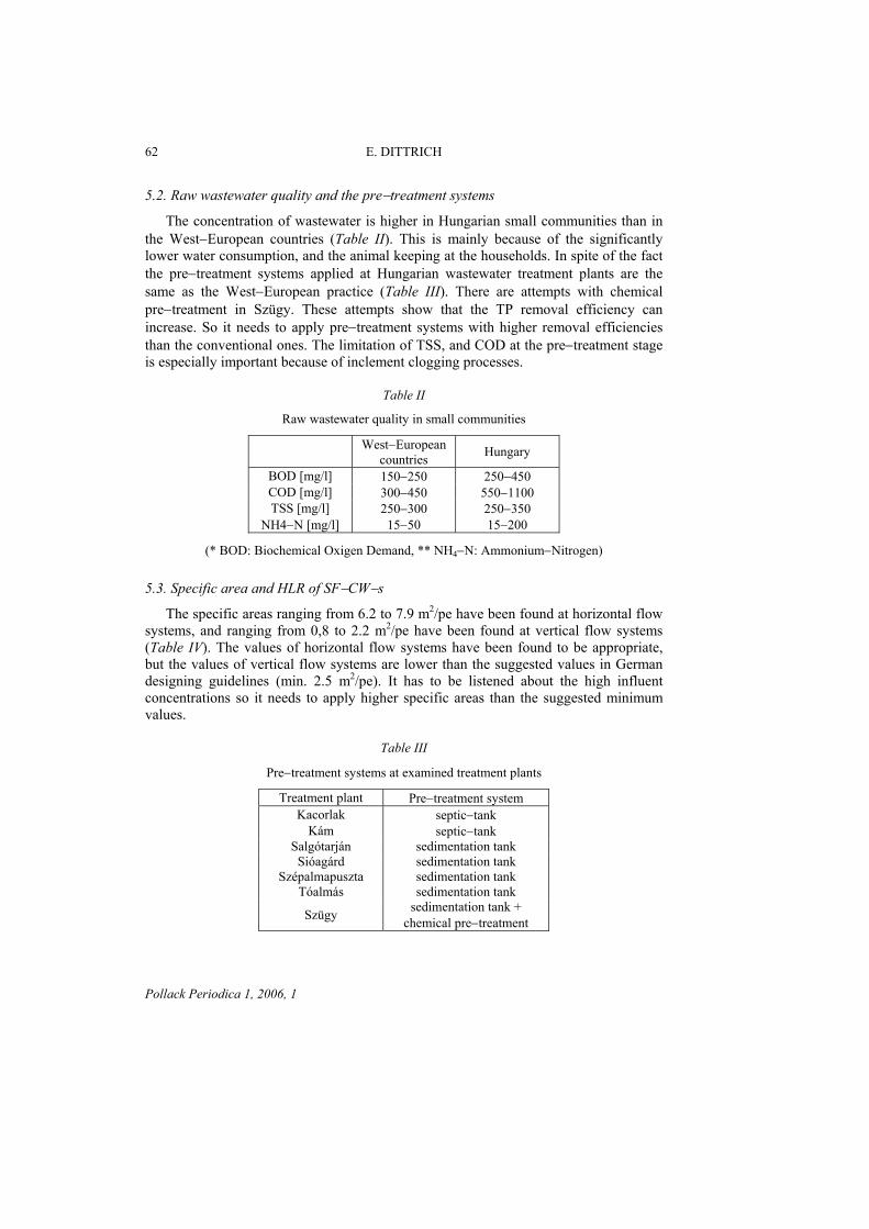
62 E. DITTRICH
5.2. Raw wastewater quality and the pre−treatment systems
The concentration of wastewater is higher in Hungarian small communities than in the West−European countries (Table II). This is mainly because of the significantly lower water consumption, and the animal keeping at the households. In spite of the fact the pre−treatment systems applied at Hungarian wastewater treatment plants are the same as the West−European practice (Table III). There are attempts with chemical pre−treatment in Szügy. These attempts show that the TP removal efficiency can increase. So it needs to apply pre−treatment systems with higher removal efficiencies than the conventional ones. The limitation of TSS, and COD at the pre−treatment stage is especially important because of inclement clogging processes.
Table II
Raw wastewater quality in small communities
West−European countries Hungary
BOD [mg/l] 150−250 250−450 COD [mg/l] 300−450 550−1100 TSS [mg/l] 250−300 250−350
NH4−N [mg/l] 15−50 15−200
(* BOD: Biochemical Oxigen Demand, ** NH4−N: Ammonium−Nitrogen)
5.3. Specific area and HLR of SF−CW−s
The specific areas ranging from 6.2 to 7.9 m2/pe have been found at horizontal flow systems, and ranging from 0,8 to 2.2 m2/pe have been found at vertical flow systems (Table IV). The values of horizontal flow systems have been found to be appropriate, but the values of vertical flow systems are lower than the suggested values in German designing guidelines (min. 2.5 m2/pe). It has to be listened about the high influent concentrations so it needs to apply higher specific areas than the suggested minimum values.
Table III
Pre−treatment systems at examined treatment plants
Treatment plant Pre−treatment system Kacorlak septic−tank
Kám septic−tank Salgótarján sedimentation tank
Sióagárd sedimentation tank Szépalmapuszta sedimentation tank
Tóalmás sedimentation tank
Szügy sedimentation tank + chemical pre−treatment
Pollack Periodica 1, 2006, 1

EXPERIENCES ON SUB−SURFACE FLOW CONSTRUCTED WETLANDS 63
The values of HLR are from 10 to 30 mm/d at horizontal flow systems, and from 73 to 100 mm/d at vertical flow systems (Table IV). The calculated values of HLR are lower than the suggested maximum values (40 mm/d) at horizontal flow systems. The calculated range of HLR is higher than the suggested maximum values (60 mm/d). So it needs to reduce the HLR at Hungarian vertical flow SF−CW−s. That shows too, it needs to grow up the specific area of vertical flow systems in Hungary.
Table IV
Specific area and HLR of examined SF−CW−s
Con
stru
ctio
n ty
pe
SF−C
W
syst
ems
Spec
ific
area
[m
2 /pe]
HLR
[cm
/day
]
Kacorlak (H.F.) 7.9 3 Horizontal flow system Kám (H.F.) 6.2 1
Salgótarján (V.F.) 1 10 Sióagárd (V.F.) 0.8 9.8
Szépalmapuszta (V.F.) 1.35 7.4 Tóalmás (V.F.) 1 10
Vertical flow system
Szügy (V.F.) 2.2 7.3
5.4. TSS−loading rate and COD−loading rate of Hungarian SF−CW−s
The specific TSS−loading rates ranging from 0.44 g/m2,d to 0.45 g/m2,d were found at examined horizontal flow systems, and from 0.44 g/m2,d to 17.4−0,44 g/m2,d at vertical flow systems (Table V). 5–7 g/m2,d is suggested as maximum value by the international literature. So the calculated TSS−loading rate is too high at Szügy and Sióagárd. The specific COD−loading values are from 3.3 to 5.1 gCOD/m2,d at horizontal flow systems, and from 5.1 to 43.3 gCOD/m2,d at vertical flow systems (Table V). The values of horizontal flow systems are appropriate but the values of vertical flow systems are higher than the suggested maximum values in international specific articles (20–25 g/m2,d). There are especially high COD−loading rates in Sióagárd and Szépalmapuszta.
5.5. Filter media at Hungarian SF−CW−s
The applied filter media is soil in the examined horizontal flow systems. These systems were built supported to Kickuth−theory. The Hungarian experiences are the same as the international ones. A big part of wastewater flows through the SF−CW−s with surface−flow [2, 28]. This is because of the low hydraulic conductivity of soil based filter media. At the vertical flow systems the applied filter media is sand 2 usually with fractions of natural grain−distribution. The filter media is clogged at the examined vertical flow
Pollack Periodica 1, 2006, 1

64 E. DITTRICH
systems. So it seems to be not a good practice because the level of fine fraction is usually too high in natural sand. It is important to limit fine fraction in the filter media (f.e.: d10>0.2 mm and U<5) to reduce the risk of clogging.
Table V
TSS− and COD−loading rates of examined SF−CW−s
Con
stru
ctio
n ty
pe
SF−C
W
syst
ems
Spec
ific
TSS−
load
ing
rate
[g/m
2 ,d]
Spec
ific
CO
D−l
oadi
ng
rate
gC
OD
/m2 ,d
]
Kacorlak (H.F.) 0.45 5.1 Horizontal flow system Kám (H.F.) 0.44 3.3
Salgótarján (V.F.) 6.6 8.8 Sióagárd (V.F.) 9.8 43.3
Szépalmapuszta (V.F.) 4 35.5 Tóalmás (V.F.) 2.8 5.1
Vertical flow system
Szügy (V.F.) 17.4 23.7
6. Conclusions
A new research with rigorous monitoring has been started to get more detailed data about real hydraulic distribution and real mixing processes in SF−CW−s. This needs more detailed data to do deeper analysis and calibrate hydraulic and transport models. The calibrated transport model could help us to work out more precise design methods. Further research is needed to get measured data and theoretical results closer to each other. Conclusions as regards the construction and operation of SF−CW−s, based on the evaluation of Hungarian data and international experiences are as follows: − The horizontal flow systems based on Kichkuth−theory does not work. So soil
should not be used as filter media. − At the design stage it needs to apply sufficiently porous media (grain with
dmin=3−5 mm) and large enough contact surfaces at the Hungarian horizontal flow systems. Darcy’s law does not work to calculate the cross sectional area because of the clogging processes.
− It needs to apply pre−treatment systems with higher TSS and COD removal efficiencies than the conventional pre−treatment systems (septic tank or sedimentation tank) in Hungary, because of the high raw wastewater concentration in Hungarian small communities.
− It is very important to use higher specific area and limitation of the hydraulic loading rate at the design stage especially at the vertical flow systems.
− It is important to limit fine fraction in the filter media (f.e.: d10>0.2 and U<5) to reduce the risk of clogging at Hungarian vertical flow systems.
Pollack Periodica 1, 2006, 1

EXPERIENCES ON SUB−SURFACE FLOW CONSTRUCTED WETLANDS 65
Acknowledgements
This work has been undertaken as a part of a project founded by the University of Pécs, Pollack Mihály Faculty of Engineering. The Author is pleased to acknowledge the data of the Department of Sanitary and Environmental Engineering at Budapest University of Technology and Economics as well as the professional advices of Ferenc Szilágyi, PhD.
References
[1] Haberl R., Perfler R., Mayer H. Constructed wetlands in Europe, Water Science and Technology, Vol. 32, No. 3. 1995, pp. 305−315.
[2] Rewiew of extensive wastewater treatment technologies, (In Hungarian) Scientific Research Report, Department of Sanitary and Environmental Engineering, Budapest University of Technology and Economic, Budapest, 2002.
[3] Haszpra O. HydraulicsII/1, (In Hungarian). Tankönyvkiadó, Budapest, 1989. [4] Kovács Gy. The hydraulics of seepage, (In Hungarian), Akadémia Kiadó, Budapest, 1972. [5] Langergraber G. Simulation of subsurface flow constructed wetlands – results and further
research needs, Water Science and Tech., Vol. 48, No. 5, 2003, pp. 157−166. [6] Kawanishi T., Kawashima H., Chihara K., Suzuki M. Effect of biological clogging on
infiltration rate in soil treatment systems, Water Science and Technology, Vol. 22, No. 3−4, 1990, pp. 101−108.
[7] Kadlec R.H. Chemical, physical and biological cycles in treatment wetland, Water Science and Technol. Vol. 40, No. 3, 1999, pp. 37−44.
[8] Fliep Gy., Kovács B., Lakatos J., Madarász T., Szabó I. Ground and groundwater treatment in polluted areas (In Hungarian) Miskolci Egyetemi kiadó, Miskolc, 2002.
[9] Tanner C.C., Sukias J.P. Accumulation of organic solids in gravel−bed constructed wetlands, Water Science and Technol. Vol. 32, No. 3, 1995, pp. 229−239.
[10] King A.C., Mitchell C.A., Howes T. Hydraulic tracer studies in a pilot scale subsurface flow constructed wetland, Water Science and Technol. Vol. 35, No. 5, 1997, pp. 189−196.
[11] Batchelor A., Loots P. A critical evaluation of a pilot scale subsurface flow wetland: 10 years after commissioning, Water Science and Technol., Vol. 35, No. 05, 1997, pp 337−343.
[12] Langergraber G., Harberl R., Laber J., Pressl A. Evaluation of substrate clogging processes in vertical flow constructed wetlands, Water Science and Technology, vol. 48, No. 5, 2003, pp. 25−34.
[13] Winter K.J., Goetz D. The impact of sewage composition on the soil clogging phenomena of vertical flow constructed wetlands, Water Science and Technology, Vol. 48, No. 5, 2003, pp. 9−14.
[14] Blazejewski R., Murat−Blazejewszka S. Soil clogging phenomena in constructed wetlands with subsurface flow, Water Science and Techn. Vol. 35, No. 5, 1997, pp 183−188.
[15] Rash J.K., Liehr S.K. Flow pattern analysis of constructed wetlands treating landfill ,Water Science and Technology, Vol. 40, No. 3, 1999, pp. 309−315.
[16] Breen P.F., Chick A.J. Root zone dynamics in constructed wetlands receiving wastewater: a comparison of vertical and horizontal format systems, Water Science and Technol. Vol. 32, No. 3, 1995, pp. 281−289.
Pollack Periodica 1, 2006, 1

66 E. DITTRICH
[17] Schierup H.H., Brix H., Lorenzen B. Wastewater treatment in constructed reed beds in Denmark – State of the art, in Constructed Wetlands in Water Pollution Control, Ed. by Cooper P.F., Findlater B.C., Pregamon Press, 1990.
[18] Kadlec R.H. Deterministic and stochastic aspects of constructed wetland performance and design, Water Science and Technology, Vol. 35, No. 5, 1997, pp. 149−156.
[19] Shilton A.N., Prasad J.N. Tracer studies of a gravel bed wetland, Water Science and Technology, Vol. 34, No. 3−4, 1996, pp. 421−425.
[20] Crites R.W. Design criteria and practice for constructed wetlands, Water Science and Technol. Vol. 29, No. 4, 1994, pp 1− 6.
[21] Laber J., Haberl R., Perfler R., Langergraber G. Influence of substrate clogging on the treatment capacity of vertical−flow constructed wetland system, 7th International Conference on Wetland Systems for Pollution Controll, Florida, 11−16 November, 2000, Vol. II., pp. 937−945.
[22] Dulovics D. Waste−water treatment technologies of small communities II. (In Hungarian) MASZESZ (Magyar Szennyvíztechnikai Szövetség) Hírcsatorna, Nov.−Dec. 2002, pp. 3−14.
[23] Weedon C.M. Compact vertical flow constructed wetland systems – first two years’ performance, Water Science and Technology, Vol. 48, No. 5, 2003, pp. 18−23.
[24] MASZESZ MI−I−1, 2003, Technical sheet of vertical flow reed bed systems, (Standard, In Hungarian), 2003.
[25] Gampel T. Operational experiences of Hungarian constructed wetlands, (In Hungarian) MHT XVIII. Országos Vándorgyűlés, Veszprém, July 5−6. 2000, vol. I. pp. 163−177.
[26] Hajdú Sz. Sub−surface flow constructed wetlands, and live−machines, (In Hungarian) Diploma Thesis, Department of Environmental Engineering, Pollack Mihály Faculty of Engineering, University of Pécs, 2002.
[27] Szilágyi F. The operational order of sub−surface flow constructed wetland treatment plant in Szügy, (In Hungarian) Vituki Consult Rt. Budapest, 1994.
[28] Lakosi I. The experiences of extensive wastewater treatment technologies in the west part of Hungary, (In Hungarian), MASZESZ Hírcsatorna, March−April, 2003, pp. 8−14.
Pollack Periodica 1, 2006, 1

POLLACK PERIODICA An International Journal for Engineering and Information Sciences
DOI: 10.1556/Pollack.1.2006.1.5 Vol. 1, No. 1, pp. 67–76, (2006)
www.akademiai.com
METHODS FOR SIMULATING HYDRODYNAMIC EFFECTS IN TRIBOTECHNICAL PROCESSES
Ivan V. ABRAMOV, 1Alexey V. SCHENYATSKY, 2Alexander A. LUZGIN
Department of Mechatronic Systems, Izhevsk State Technical University No.7 Studencheskaya str., 426069 Izhevsk, Russia e−mail: [email protected], [email protected]
Received 20 October 2005; accepted 06 April 2006
Abstract: In this paper variational and analytical methods for the solution of multilinked contact mechanical problems of deformable solids and fluid have been considered. Numerical methods have been found cumbersome and inaccurate. In this connection a new accurate and quick variational−analytical method for the lubricant flow analysis has been developed. Keywords: Hydraulic pressure, Hydrodynamics, Interference−fit joint, Mode of deformation, Viscous fluid flow
1. Introduction
Nowadays interference−fit joints are widely used for transmitting axial forces and torques varied by direction and magnitude. Their use with continuously increasing loads requires increasing their load capacity and strength. Thus obtaining a joint with the maximum strength and required operational effectiveness is a very important problem for modern machinery. One of the most efficient technological methods for joints load capacity increase is female parts elastoplastic deformation (ED). It is implemented under conditions of dry, liquid and boundary friction types. At the same time, one of the most efficient ways to assemble an interference−fit joint is using the hydraulic assembly method, which is carried out in the liquid friction mode. Performing the processes in the liquid friction mode provides the following advantages: press force reduction with the same productivity, mating parts safety; there is no micro asperities smashing, hence increase the actual contact area and mating
HU ISSN 1788−1994 © 2006 Akadémiai Kiadó, Budapest

68 I.V. ABRAMOV, A.V. SCHENYATSKY et al.
surfaces friction ratio in the designed joint. Changing the press speed, geometrical and material properties of the parts, rheological properties of the lubricant, using various lubricant supply schemes and pressure gain methods allow controlling the resulting shapes of the parts and their residual mode of deformation. In this connection hydrodynamic effects simulation allowing for the mentioned factors will help determine the best technological modes for the process and hence control the properties of the resulting joint. The feature of the ED process in the liquid friction mode is that the surfaces of the parts are being deformed under the influence of pressure in a thin and long lubricating layer with non−constant height. At each time step of the whole process the analysis is done in several phases: a) the lubricant pressure values distribution is calculated first; b) the lubricant pressure forces are then applied onto the surfaces of the parts; c) the elastoplastic mechanical problem of deformable solids is being solved using the finite element method (FEM). As all numerical methods, FEM allows to solve complex differential tasks by just solving a linear equations set. As a result nodal displacements and the mode of deformation parameters’ values are calculated.
2. The investigated model
Pressure distribution in a thin and long lubricating layer has been analyzed by means of analytical and variational methods [1, 2, 3, 4]. Experimental methods are expensive and unprofitable. Analytical methods are applicable just for simple shapes of the parts and the clearance. But in a real process the parts and the clearance shapes are changing unpredictably. Using FEM [5] and other numerical methods for the fluid mechanical problem in the present task provides rather inaccurate results because the height of the analyzed fluid layer is very low comparing to its length. For an ED process the typical height−to−length ratio value interval is 35 105,7105,7 −− ⋅≤≤⋅ lh . Analyzing fluid flow between two parts by means of the finite difference method (FDM) [6] allowed determining the influence of design of the joint and assembly technology on the contact pressure distribution along the joint, mode of deformation and find risk areas with their maximum stresses. The analysis of the hydro−press joint assembly method (Fig.1), that involves the same physical processes as in ED process in the liquid friction mode, has showed that the parts are being separated by a thin lubricating layer maintained by an external pressure source. In the mating zone the parts are being affected by contact pressures occurring there due to the difference in the mounting dimensions of the parts and hydrodynamic pressure in the lubricating layer of non−constant height. From the outer side the parts are affected by technological rigging providing a qualitative assembly process [3]. When analyzing the contact of parts and fluid, multilinked contact conditions must be taken into account. The presence of metallic layers, applied onto the joint’s elements, is considered when composing the resolving linear equations set, which in the FEM formulation [4] is as follows:
Pollack Periodica 1, 2006, 1

SIMULATING HYDRODYNAMIC EFFECTS IN TRIBOTECHNICAL PROCESS 69
[ ]{ } { } { } { } { } { }[ ]{ } { } ,0
,0 *
00=−
=−++++
Φδ
δ σεH
RFFFFK iiibipiii (1)
where K and H – the coefficient matrixes of the equations set,
i is an index,
⎪⎪⎪⎪
⎩
⎪⎪⎪⎪
⎨
⎧
=
part,maletheaffectingrigging,thefor6,part,femaletheaffectingrigging,thefor5,
part,maletheonlayermetallic4,part,femaletheonlayermetallic3,
part,malethefor2,part,femalethefor1,
i
{ }⎭⎬⎫
⎩⎨⎧
=izir
i xx
δ is nodal displacements in the finite−element grid,
{ } { } { } { }00
,,, σε iibipi FFFF is nodal forces due to distributed (with the index p) and
boundary (with the index b) loads, initial strains (with the index 0ε ) and initial stresses (with the index 0σ ).
Fig. 1. An interference−fit joint’s parts and rigging for hydro−press assembly
1–shaft; 2–bush; 3–work tool; 4–false shaft
The elements in the second equation of the system (1) are
is the velocities and the pressure vector, { }⎪⎭
⎪⎬
⎫
⎪⎩
⎪⎨
⎧=
k
zk
rk
kpvv
*δ
is the vector of mass forces. { }ΦThe influence of resistance forces and inertias, according to the D’Alembert’s principle, is replaced by their static equivalent. Forces affecting the parts surfaces in their interfacing zone, occurred there due to the contact pressure, are equal by magnitude and opposite by direction
Pollack Periodica 1, 2006, 1

70 I.V. ABRAMOV, A.V. SCHENYATSKY et al.
. (2) { } { }21 FF −=
Under the forces influence the mating surfaces are moving (Fig. 2). Their displacements depend on the interference value
iiririiii xxxhN ζ∆ λ +∑+±=−+ 2121
m (3)
where is the interference of the analyzed joint, is the lubricating layer height, is the gap size, only for joints assembled by auto−fastening and auto−frettage,
and are the nodal radial displacements of the female part, the first case (
and ) conforms to assembling with an interference, the second one (
and ) conforms to assembling with a gap, is the total contact juncture
ductility,
iN ih
i∆ rix1
rix2 01 >rix
02 <rix 01 <rix
02 >rix ∑ ixλ
iζ is the allowed displacements computing error. N
i/2hi
x2ix1
i
Fig. 2. Displacements consistency conditions in HPJ (assembling with autofrettage)
The pressure distribution in the lubricating layer is calculated after the solution of the fluid mechanical problem for known geometry of the clearance geometry. Forces in the contact zone are determined as
(4) ( ){ }
⎪⎪⎪⎪⎪
⎩
⎪⎪⎪⎪⎪
⎨
⎧
−∫
−∫
⎩⎨⎧
−∫∫
−∫
=
zone.friction liquidfor force axial,}{][
zone,friction liquidfor force radial ,}{][
zone,friction mixed anddry for force axial
,}{][or )(}{][
zone,friction mixed anddry for force radial the ,}{][
,
SLT
SLT
SCpT
SKT
SKT
KMki
dStB
dSpN
dStBdSpfpN
dSpN
ppF
The forces, clearance dimensions and fluid flow speed values are computed using an iterational method for solving the equations set (1). Contact pressure, the mode of deformation of the parts in an assembled joint are determined allowing for the parts
Pollack Periodica 1, 2006, 1

SIMULATING HYDRODYNAMIC EFFECTS IN TRIBOTECHNICAL PROCESS 71
loading history when assembling. The lubricating layer removed in the end is not considered. Explorations [1, 2, 3] showed that in a hydro−press assembly process the maximum pressure gradient value is located at the butt of the joint, because there the clearance shape resembles a parabola. At all other locations the clearance shape resembles a wedge with a negligible obliquity. The pressure gradient value depends on the insertion length. The change in the rigging hollow length with the invariable chamfer, hollow height, assembly speed and productivity showed that the pressure changes only in the inlet, while in the outlet it mostly remains constant. If the hollow length is negligible, the inlet pressure value is 192 MPa. This value is obtained for a joint with a female part containing a chamfer of 2.5 mm size and 45º angle. The chamfer reduction will result in the pressure increase. If the hollow length equals to 5 mm, the pressure decreases to 180 MPa, or to 176 MPa if the hollow length value is 7.5. The hollow length increase up to 10–15 mm results in the pressure decrease down to 175.6–174.8 MPa
The mode of deformation computation showed that the presence of a 45º angle chamfer on the female part results in the pressure increase both in the rigging hollow and in the parts mating zone. That conditions a significant change in the mode of deformation of the part, in comparison with longitudinal pressing or hydrostatic lubricant distributing (Fig. 3).
a)
b)
Fig.3. Stress intensity field in the parts of a joint assembled using
a) press and b) hydro−press methods, a) friction coefficient f0=0.23; lins=50 mm, b) lubricant pressure is hydrostatic, Рм=126 MPa, insertion length lins=50 mm,
hollow length lHol=0.0 mm
Pollack Periodica 1, 2006, 1

72 I.V. ABRAMOV, A.V. SCHENYATSKY et al.
The performed extensive studies allowed determining the influence of chamfers in design of the female part on the assembly process parameters: lubricant pressure and press force (Fig. 4).
100
120
140
160
180
200
220
240
260
280
300
0 0,5 1 1,5 2 2,5Chamfer length, mm
Pres
sure
, MPa
I
II
III
IV
Fig. 4. The influence of chamfers in design of the female part on the lubricant pressure,
(hollow length l=5 mm, pump productivity Q=0,37 10-5 m3/s, assembly speed υ =4,0 10-3 m/s, viscosity sPa ⋅=µ )
I – both inlet chamfers are being changed, II – both outlet chamfers are being changed, III – one inlet chamfer is being changed, IV – one outlet chamfer is being changed
The diagrams analysis shows that using chamfers in the female part structure allows controlling the pressure and hence the mode of deformation of the parts and the load carrying capacity of the joint. Developed mathematical model of an assembly process helped determine the influence of the technological rigging pressing force on the assembly parameters and the mode of deformation of the parts. Hydro−press joints (HPJ) load−carrying capacity analysis showed that when assembling at high contact and fluid pressure values that exceed the yield point, the residual interference and contact pressure change occurs. The HPJ load carrying capacity is then lower than if it was assembled using the thermal method.
3. The applied method
Variational methods application to the concerned problem showed that multilinked contact problems solution involves consuming a long−time and high system requirements. And so, taking into account the complication of FEM and FDM application to fluid mechanics two−directional problem [7], a variational−analytical solution method has been developed. The fluid flow in a thin lubricant layer between the mating surfaces is performed with low assembling (deforming) speed values. Hence the fluid flow can be considered to occur at low Reynolds numbers. For the present task we can use the steady
Pollack Periodica 1, 2006, 1

SIMULATING HYDRODYNAMIC EFFECTS IN TRIBOTECHNICAL PROCESS 73
Newtonian viscous fluid flow model governed by the Navier−Stokes differential equations set [8]. The used assumptions are: fluid flows mostly in the axial direction, the component
rυ value is much lower than zυ ; fluid sticks to the walls, zυ is changing much slower than rυ . The following set of approximating equations can be obtained from the initial equations
( ).01
,0
,11
=∂∂
+∂
∂
=∂∂
∂∂
=⎟⎠
⎞⎜⎝
⎛∂∂
∂∂
zrr
r
rp
zp
rr
rr
zr
z
υυ
µυ
(5)
To investigate the fluid flow in the layer with non−constant height we split it into a number of simple−shaped regions (Fig. 5).
p=p0 p=p0
z
rfemale part
male part
1 (1) 2 (2) 3 i (i) i+1 m (m) n
z2 z3 zi z i+1 zm znz1
Fig. 5. Lubricating layer split into simple−shaped regions
Such a shape of a region can be easily and accurately enough approximated by a simple function. As a result the lubricating layer is represented by a sequence of m simple regions confined by n=m+1 sections ( ,m n N∈ ). In Fig. 5 a number in round brackets defines a region, and a number without brackets defines a section. The insertion direction is supposed to be opposite to the z−coordinate axis direction. Then the following boundary conditions conform to each region i (here and further
1,i m= ).
( )( ) ,0 ,0 then , , if
,0 , then , , if
1
1
==≤≤=
=−=≤≤=
+
+
rziii
rziii
vvzzzzbr
vUvzzzzar (6)
Pollack Periodica 1, 2006, 1
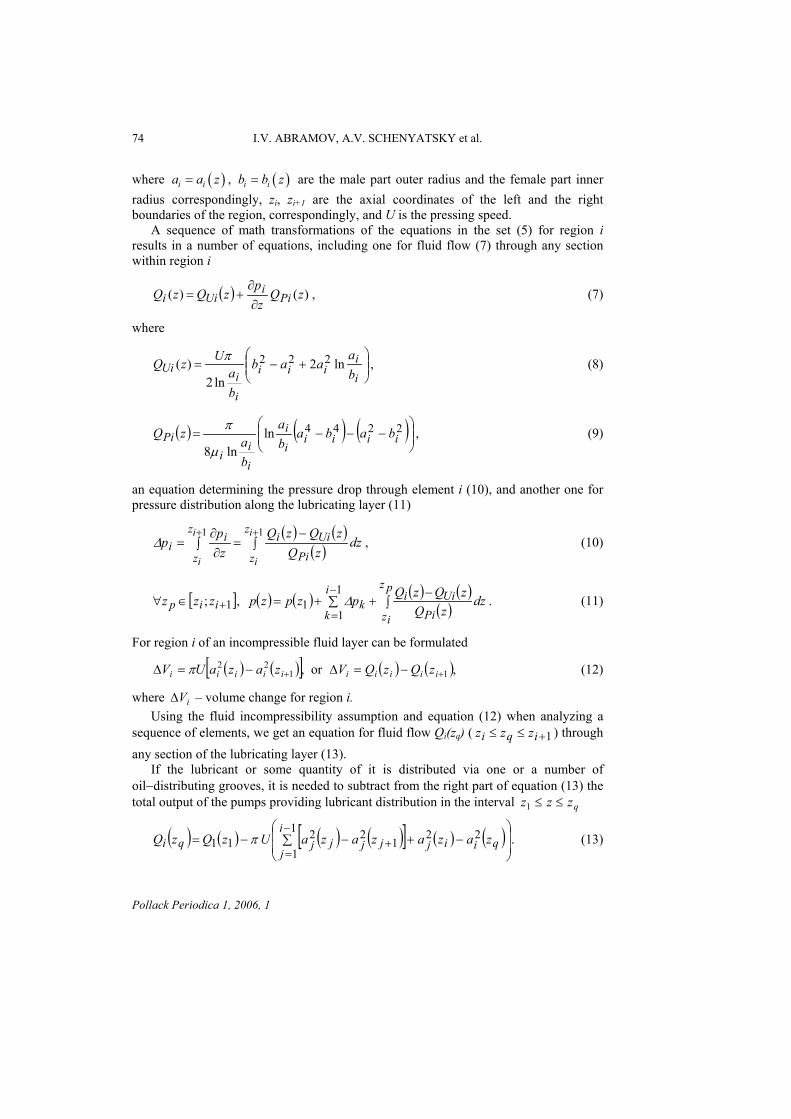
74 I.V. ABRAMOV, A.V. SCHENYATSKY et al.
where , are the male part outer radius and the female part inner radius correspondingly, z
( )i ia a z= ( )i ib b z=
i, zi+1 are the axial coordinates of the left and the right boundaries of the region, correspondingly, and U is the pressing speed. A sequence of math transformations of the equations in the set (5) for region i results in a number of equations, including one for fluid flow (7) through any section within region i
( ) )()( zQz
pzQzQ Pi
iUii ∂
∂+= , (7)
where
⎟⎟⎠
⎞⎜⎜⎝
⎛+−=
ii
iii
ii
Ui ba
aab
ba
UzQ ln2ln2
)( 222π , (8)
( ) ( ) ( )⎟⎟⎠
⎞⎜⎜⎝
⎛−−−= 2244ln
ln8iiii
ii
ii
iPi baba
ba
ba
zQµ
π , (9)
an equation determining the pressure drop through element i (10), and another one for pressure distribution along the lubricating layer (11)
( ) ( )
( )∫ ∫−
=∂∂
=+ +1 1i
i
i
i
z
z
z
z PiUiii
i dzzQ
zQzQz
pp∆ , (10)
[ ] ( ) ( ) ( ) ( )( )∑ ∫
−++=∈∀
−
=+
1
111 ,;
i
k
pz
iz PiUii
kiip dzzQ
zQzQpzpzpzzz ∆ . (11)
For region i of an incompressible fluid layer can be formulated
( ) ( )[ ] ( ) ( ),or, 1122
++ −=∆−=∆ iiiiiiiiii zQzQVzazaUV π (12)
where – volume change for region i. iV∆ Using the fluid incompressibility assumption and equation (12) when analyzing a sequence of elements, we get an equation for fluid flow Qi(zq) ( ) through any section of the lubricating layer (13).
1+≤≤ iqi zzz
If the lubricant or some quantity of it is distributed via one or a number of oil−distributing grooves, it is needed to subtract from the right part of equation (13) the total output of the pumps providing lubricant distribution in the interval qzzz ≤≤1
(13) ( ) ( ) ( ) ( )[ ] ( ) ( ) .1
122
122
11 ⎟⎟
⎠
⎞
⎜⎜
⎝
⎛∑ −+−−=−
=+
i
jqiijjjjjqi zazazazaUzQzQ π
Pollack Periodica 1, 2006, 1
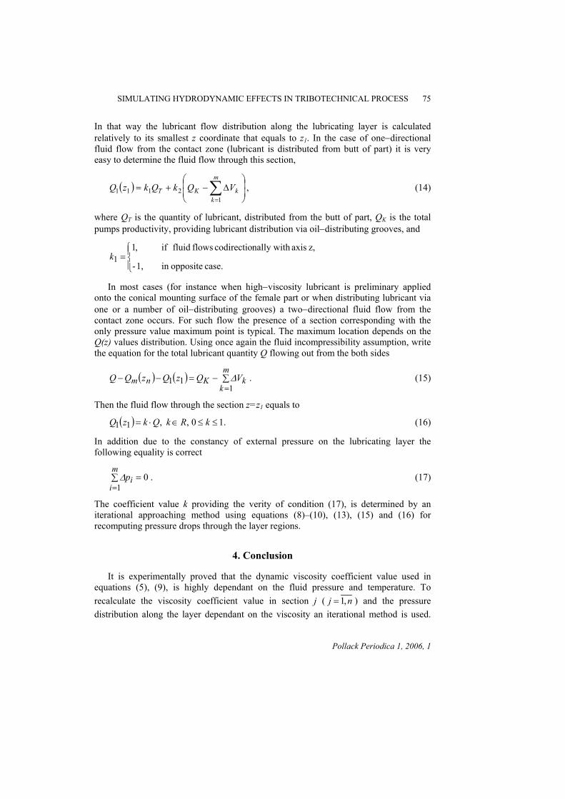
SIMULATING HYDRODYNAMIC EFFECTS IN TRIBOTECHNICAL PROCESS 75
In that way the lubricant flow distribution along the lubricating layer is calculated relatively to its smallest z coordinate that equals to z1. In the case of one−directional fluid flow from the contact zone (lubricant is distributed from butt of part) it is very easy to determine the fluid flow through this section,
, (14) ( ) ⎟⎟⎠
⎞⎜⎜⎝
⎛∆−+= ∑
=
m
kkKT VQkQkzQ
12111
where QT is the quantity of lubricant, distributed from the butt of part, QK is the total pumps productivity, providing lubricant distribution via oil−distributing grooves, and
⎪⎩
⎪⎨⎧
=case. oppositein 1,-
z, axis nally withcodirectio flows fluid if,11k
In most cases (for instance when high−viscosity lubricant is preliminary applied onto the conical mounting surface of the female part or when distributing lubricant via one or a number of oil−distributing grooves) a two−directional fluid flow from the contact zone occurs. For such flow the presence of a section corresponding with the only pressure value maximum point is typical. The maximum location depends on the Q(z) values distribution. Using once again the fluid incompressibility assumption, write the equation for the total lubricant quantity Q flowing out from the both sides
. (15) ( ) ( ) ∑−=−−=
m
kkKnm VQzQzQQ
111 ∆
Then the fluid flow through the section z=z1 equals to
( ) .10,,11 ≤≤∈⋅= kRkQkzQ (16)
In addition due to the constancy of external pressure on the lubricating layer the following equality is correct
. (17) ∑ ==
m
iip
10∆
The coefficient value k providing the verity of condition (17), is determined by an iterational approaching method using equations (8)–(10), (13), (15) and (16) for recomputing pressure drops through the layer regions.
4. Conclusion
It is experimentally proved that the dynamic viscosity coefficient value used in equations (5), (9), is highly dependant on the fluid pressure and temperature. To recalculate the viscosity coefficient value in section j ( nj ,1= ) and the pressure distribution along the layer dependant on the viscosity an iterational method is used.
Pollack Periodica 1, 2006, 1

76 I.V. ABRAMOV, A.V. SCHENYATSKY et al.
Approaching continues until two neighbor iterations’ values divergence does not exceed 1 %. Dynamic viscosity coefficient values within each region are approximated linearly depending on the viscosity values in the region’s boundary sections. The suggested math model of a fluid flow in a thin and long circular gap between the parts of an assembled joint is implemented as a program application. Extensive studies showed the high accuracy and speed of the algorithm, that are high advantages comparing to numerical methods. The suggested model adequacy is confirmed experimentally and in comparison with the results of a computation performed using an analytical method for a simple−shaped gap, considered in [8]. The divergence of the results was less than 10-4 %. It is ascertained that the results accuracy obtained by the suggested method depends on: compliance of the process conditions with the assumptions used for the derivation of differential equations set (5), the accuracy of the lubricating layer shape approximation by the functions ai=ai(z), bi=bi(z). Depending on the functions ai and bi types, the application of a numerical integrating method might be needed when using equations (10) and (11). The chosen integrating method also affects the computing accuracy. The suggested analytical method allows to: a) productively and very accurately analyze the hydrodynamic effects occurring in the lubricating layer, and hence choose the best parameters and modes for hydro−press joints assembling and female parts ED processes using parts with any shapes and dimensions, b) analyze high−strength joints with guaranteed interferences at any life cycle phase, except for disposal, c) determine the load−carrying capacity of the joint or deformed part allowing for a technological factor influence and calculate the parameters for technological processes with various contact events occurring in joints (parts) assembled (deformed) using various methods.
References [1] Schenyatsky A.V., Abramov I.V. On the problem of hydraulic interference−fit joint theory,
5th International Conference on Dynamics of the Machine Aggregates 2000, Gabčikovo, Slovac Republic, 2000. pp. 183−188.
[2] Schenyatsky A.V., Sosnovich E.V. Load factors determination features in hydraulic interference−fit joints numerical modeling, ХХХI Scientific−Technical Conference on IzhGTU, (In Russian) 15−17 April 1998. Ishevsk, Vol. 2, pp. 217−219.
[3] Schenyatsky A.V., Sosnovich E.V. Hydro−press assembly parameters determination allowing for the lubricant layer distribution mechanism, Vestnik IzhGTU, (In Russian) Vol. 2. Izhevsk, IshGTU, 1998. pp. 22−23.
[4] Kholmogorov G.L., Malinina T.S. Newtonian lubricant flow in a thin drawing process in the liquid friction mode, Trenie i iznos, (In Russian) 1992, Vol. 13, No. 5, pp. 811−815.
[5] Zinkiewicz O.C. The finite element method in engineering science, Translation from English (In Russian) Edited by B.E. Pobedri, Moscow, Mir, 1975.
[6] Tenenev V.A., Rusyak I.G. The numerical solution of hydrodynamics and thermal problems for complex−shaped areas, Methodical Literature, (In Russian) IzhGTU, Dep. of Applied Math. Izhevsk, IzhGTU, 1996.
[7] Ershov N.F., Shahverdi G.G. The finite elements method in hydrodynamics and hydroelasticity problems, (In Russian) Leningrad, Sudostroenie, 1984.
[8] Targ S.M. Basic laminar flow problems, (In Russian) Moscow, Mashgiz, 1961.
Pollack Periodica 1, 2006, 1

POLLACK PERIODICA An International Journal for Engineering and Information Sciences
DOI: 10.1556/Pollack.1.2006.1.6 Vol. 1, No. 1, pp. 77–92, (2006)
www.akademiai.com
OPTIMUM DESIGN OF STIFFENED PLATES
Zoltán VIRÁG
Department of Equipments for Geotechnics, University of Miskolc, H−3515, Miskolc−Egyetemváros, Hungary, e−mail: gtbvir@uni−miskolc.hu
Received 2 January 2006; accepted 12 March 2006
Abstract: In this overview of loaded stiffened plates various types, loadings, and stiffener shapes are investigated. Mikami and API methods are used for the optimum design and comparison of the two methods. Both methods consider the effect of initial imperfection and residual welding stresses, but their empirical formulae are different. The elastic secondary deflection due to compression and lateral pressure is calculated using the Paik’s solution of the differential equation for orthotropic plates, and the self−weight is also taken into account. The unknowns are the thickness of the base plate as well as the dimensions and number of stiffeners. The cost function to be minimized includes two kinds of material and three kinds of welding costs. Keywords: Stiffened plate, Welded structures, Stability, Residual welding distortions, Structural optimisation, Minimum cost design
1. Introduction
Welded stiffened plates are widely used in various load−carrying structures, e.g. ships, bridges, bunkers, tank roofs, offshore structures, vehicles, etc. They are subject to various loadings, e.g. compression, bending, shear or combined load. The shape of plates can be square rectangular, circular, trapezoidal, etc. They can be stiffened in one or two directions with stiffeners of flat, L, trapezoidal or other shape. Various types, loadings, stiffener shapes have been investigated. In this paper two kinds of loads are investigated [1], [2]. These are the uniaxial compression and the lateral pressure. Structural optimisation of stiffened plates has been worked out by
HU ISSN 1788−1994 © 2006 Akadémiai Kiadó, Budapest

78 Z. VIRÁG
Farkas [3], Farkas and Jármai [4], and applied to uniaxially compressed plates with stiffeners of various shapes [5], biaxially compressed plates [6]. This paper contains the minimum cost design of longitudinally stiffened plates using the strength calculation methods. Deflections due to lateral pressure, compression stress and shrinkage of longitudinal welds are taken into account in the stress constraint. The self−weight is added to the lateral pressure. The local buckling constraint of the base plate strips is formulated as well. The cost function includes two kinds of material and three kinds of welding costs. The unknowns are the thickness of the base plate as well as the dimensions and number of stiffeners.
2. Geometric characteristics
The stiffened plates are shown in Figs. 1, 2. The plates are simple supported on four edges. Geometrical parameters of plates with flat−, L− and trapezoidal stiffeners can be seen in Fig. 3.
Fig. 1. Longitudinally stiffened plate loaded by uniaxial compression
Fig. 2. Longitudinally stiffened plate loaded by uniaxial compression and lateral pressure
Pollack Periodica 1, 2006, 1
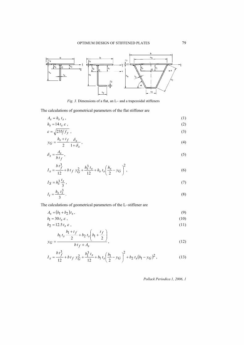
OPTIMUM DESIGN OF STIFFENED PLATES 79
Fig. 3. Dimensions of a flat, an L− and a trapezoidal stiffeners
The calculations of geometrical parameters of the flat stiffener are
, (1) sss thA = ε 14 ss th = , (2)
yf235=ε , (3)
s
sfsG
thy
δδ+
+=
12, (4)
fs
s tbA
=δ , (5)
23
23
2
12
12
⎟⎠
⎞⎜⎝
⎛ −+++= Gs
ssss
Gff
x yhththytbtb
I , (6)
3
3 ssS
thI = , (7)
3 3ss
tthI = . (8)
The calculations of geometrical parameters of the L−stiffener are
, (9) ( ss tbbA 21 += ) ε 301 stb = , (10) ε 5.122 stb = , (11)
sf
fs
fs
G Atb
tbtb
tbtb
y+
⎟⎟⎠
⎞⎜⎜⎝
⎛++
+
=
2
2 12
11
, (12)
( 212
21
1312
3
2
12
12
GsGs
sGf
fx ybtbybtb
tbytb
tbI −+⎟
⎠⎞
⎜⎝⎛ −+++= ) , (13)
Pollack Periodica 1, 2006, 1

80 Z. VIRÁG
ss
S tbbtb
I 3
221
31 += , (14)
3
3 3231 ss
ttbtbI += . (15)
The calculations of geometrical parameters of the trapezoidal stiffener are
, (16) ( sS taaA 2 21 += )
mm 300a ,90 31 ==a , thus
( ) 21222 105−= ahs , (17)
2
22 1051sin ⎟⎟
⎠
⎞⎜⎜⎝
⎛−=
aα , (18)
( ) ( )SF
FssFssG Atb
thtathtay+
+++=
2 22 21 , (19)
,2
2sin 61
2
12
2
2232
12
3
⎟⎠⎞
⎜⎝⎛ −
+++
+⎟⎠⎞
⎜⎝⎛ −+++=
GFs
ss
GF
ssGFF
x
ythtata
ythtaytbtb
I
α
(20)
α2323
231 sin sssS tathaI += . (21)
∑
=ii
pt tb
AI
24, (22)
ssp haa
hA 1952
31 =+
= . (23)
3. Design constraints in case of uniaxial compression
The stability investigation is divided into three analyses. It is practical to perform all of the analyses because of finding the dominant constraint.
3.1. Global buckling of the stiffened plate
According to Mikami [7] the effect of initial imperfections and residual welding stresses is considered by defining buckling curves for a reduced slenderness (Fig. 4)
( ) 21cryf σλ = . (24)
Pollack Periodica 1, 2006, 1

OPTIMUM DESIGN OF STIFFENED PLATES 81
The classical critical buckling stress for a uniaxially compressed longitudinally stiffened plate is
⎟⎟⎠
⎞⎜⎜⎝
⎛++
+= 2
22
21 R
Rs
cr BhD α
αγπσ , for ( ) 41
0 1 sRR BL γαα +=<= , (25)
( )[ ]212
211
2
scr BhD γπσ ++= , for 0RR αα ≥ . (26)
Fig. 4. Global buckling curve considering the effect of initial imperfections ( ) and
residual welding stresses ( ), where
00 ≠a
0≠Rσ yfUσχ =
Knowing the reduced slenderness the actual global buckling stress can be calculated according to Mikami as follows
1=yU fσ , for 3.0≤λ , (27)
( 3.063.01 −−= λσ yU f ) , for 13.0 ≤≤ λ , (28)
( )28.01 λσ +=yU f , for λ≤1 . (29)
The global buckling constraint is
s
spUA
Nδ
δρσ
+
+≤
1, (30)
where
, (31) ( ) Sf AtBA 1 −+= ϕ
f
Ss tb
A
=δ , (32)
and the factor is pρ
, if , (33) 1=pρ UUp σσ >
Pollack Periodica 1, 2006, 1

82 Z. VIRÁG
fUpp fσρ = if . (34) UUp σσ <
According to API [8] (Fig. 5)
1=yU fσ , for 5.0≤λ , (35)
λσ −= 5.1yU f , for 15.0 ≤≤ λ , (36)
λσ 5.0=yU f , for λ<1 . (37)
Fig. 5. Global buckling curve according to Mikami and API, where yfUσχ =
The global buckling constraint is UAN σ≤ . In most cases Mikami method gives thinner basic plates than that of API.
3.2. Single panel buckling
This constraint eliminates the local buckling of the base plate parts between the stiffeners. From the classical buckling formula for a simply supported uniformly compressed in one direction
22
92.104
⎟⎠⎞
⎜⎝⎛=
btE F
crPπσ , (38)
the reduced slenderness is
ε
πλ 8.5692.10
421
2 FFy
ptb
tb
fE
=⎟⎟⎠
⎞⎜⎜⎝
⎛= ,
21235
⎟⎟⎠
⎞⎜⎜⎝
⎛=
yfε , (39)
and the actual local buckling stress considering the initial imperfections and residual welding stresses is
1=yUP fσ , for , (40) 526.0≤pλ
Pollack Periodica 1, 2006, 1

OPTIMUM DESIGN OF STIFFENED PLATES 83
7.0
526.0⎟⎟⎠
⎞⎜⎜⎝
⎛=
pyU f
λσ , for , (41) pλ≤526.0
The single panel buckling constraint is
UAN σ≤ . (42)
3.3. Local and torsional buckling of stiffeners
These instability phenomena depend on the shape of stiffeners and will be treated separately for stiffener L. The torsional buckling constraint for open section stiffeners is
UTAN σ≤ . (43)
The classical torsional buckling stress is
pp
TcrT IL
IEIIG
2ωσ += , (44)
where G = E/2.6 is the shear modulus, IT is the torsional moment of inertia, IP is the polar moment of inertia and Iω is the warping constant. The actual torsional buckling stress can be calculated in the function of the reduced slenderness
( ) 21crTyT f σλ = , (45)
1=yUP fσ , for 45.0≤Tλ , (46)
( )45.053.01 −−= TyU f λσ , for 41.145.0 ≤≤ Tλ , (47)
21 TyU f λσ = , for Tλ≤41.1 . (48)
4. Design constraints in case of uniaxial compression and lateral pressure
4.1. Calculation of the deflection due to compression and lateral pressure Paik et al [9] have used the differential equations of large deflection orthotropic plate theory and the Galerkin method to derive the following cubic equation for the elastic deflection Am of a stiffened plate loaded by uniaxial compression and lateral pressure
(49) 0432
23
1 =+++ CACACAC mmm
where
Pollack Periodica 1, 2006, 1

84 Z. VIRÁG
,16
3
,16
33
422
33
421
⎟⎟⎠
⎞⎜⎜⎝
⎛+=
⎟⎟⎠
⎞⎜⎜⎝
⎛+=
BLE
LBmEAC
BLE
LBmEC
xom
x
π
π
(50a)
,
2
8
3
2
3
422
33
4223
⎟⎟⎠
⎞⎜⎜⎝
⎛++++
+⎟⎟⎠
⎞⎜⎜⎝
⎛+=
BLD
BLmH
LBmD
tLBm
BLE
LBmEAC
yxFxav
xom
πσ
π
(50b)
ptBL
LBmAC
Fxavom
164
24 π
σ −= , (50c)
⎟⎟⎠
⎞⎜⎜⎝
⎛+=
Fs
x tBAnEE 1 . (51)
Since the self−weight is taken into account the lateral pressure is modified as
LBgVpp
0ρ
+= , (52)
where g is the gravitation constant, 9.81 [m/s2]. The flexural and torsional stiffness of the orthotropic plate are as follows:
( ) ( )22
2
2
3
112
1
112
xy
x
xy
GF
xy
Fx
IEytEtED
ννν −+
−+
−= , (53)
2
12
3 23
12
86.0⎟⎠⎞⎜
⎝⎛
−⎟⎟⎠
⎞⎜⎜⎝
⎛++
=
xEEx
FtExGF
F
xx
bIE
bIE
ytEtE
EE
vν , (54)
xx
y vEE
=ν , yxxy ννν = , (55)
b
IGH txy = , ( )xy
xyEGν+
=12
, (56)
Fsi
ita
taa
tb 321 2
+∑+
= . (57)
The deflection due to lateral pressure is
Pollack Periodica 1, 2006, 1

OPTIMUM DESIGN OF STIFFENED PLATES 85
x
om IELqA 38
5 4= , , bpq = ϕBb = . (58)
The solution of Eq. (49) is
2112
3kk
CCAm ++−= , (59)
where
332
1 2742XYYk ++−= , 3
322 2742
XYYk +−−= , (60)
21
22
13
3C
CCC
X −= , 14
21
3231
32
3
27
2CC
CCC
C
CY +−= . (61)
So if the geometrical parameters, the basic material and the loads are known, the elastic deflection Eq. (59) is calculable relatively easily.
4.2. Deflection due to shrinkage of longitudinal welds
According to [4] the deflection of the plate due to longitudinal welds is as follows
8 2max LCf = , (62)
where the curvature for steels is
xTT IyQC 10844.0 3−⋅= , (63)
where QT is the heat input, yT is the weld eccentricity
2FGT tyy −= , (64)
and Ix is the moment of inertia of the cross−section containing a stiffener and the base plate strip of width b. The heat input for a stiffener is
. (65) 2 5.592 wT aQ ⋅=
4.3. Stress constraint
The stress constraint includes several effects as follows: the average compression stress and the bending stress caused by deflections due to compression, lateral pressure and the shrinkage of longitudinal welds.
UPGx
xav yIM σσσ ≤+=max , (66)
where
Pollack Periodica 1, 2006, 1

86 Z. VIRÁG
( )8 2
max0LqfAAM mmxav +++=σ . (67)
According to [7], the calculation of the local buckling strength of a face plate strip of width
( 33 ,max ababI )−= (68)
is performed taking into account the effect of initial imperfections and residual welding stresses
,526.0when,526.0
,526.0when,7.0
≥⎟⎟⎠
⎞⎜⎜⎝
⎛=
≤=
pp
UP
pyUP f
λλ
σ
λσ
(69)
where
ε
πλ 8.5692.10
4 1121
2 FFy
ptb
tb
fE
=⎟⎟⎠
⎞⎜⎜⎝
⎛= . (70)
So knowing the slenderness the critical stress is calculable, which must be higher then the maximum stress.
5. Cost function
The objective function to be minimized is defined as the sum of material and fabrication costs
, (71) ∑+=+= ifmfm TkVkKKK ρ
or in another form
( 321 TTTkk
VkK
m
f
m+++= ρ ) , (72)
where ρ is the material density, V is the volume of the structure, Km and Kf as well as km and kf are the material and fabrication costs as well as cost factors, respectively, Ti are the fabrication times as follows: time for preparation, tacking and assembly
VT d 1 ρκΘ= , (73)
where dΘ is a difficulty factor expressing the complexity of the welded structure, κ is the number of structural parts to be assembled
Pollack Periodica 1, 2006, 1
OPTIMUM DESIGN OF STIFFENED PLATES 87
T2 is time of welding, and T3 is time of additional works such as changing of electrode, deslagging and chipping. 23 3.0 TT ≈ , thus
, (74) ∑=+ winwii LaCTT 3.1 232
where Lw is the length of welds, the values of can be obtained from formulae or diagrams constructed using the COSTCOMP [10] software, a
nwii aC 2
w is the weld dimension (Table I).
Table I
Welding times in function of weld size aw (mm) for longitudinal fillet welds down−hand position
Welding technology aw [mm] 103C2awn
Submerged Arc Welding (SAW) 0−15 0.2349aw2
Shielded Metal Arc Welding (SMAW) 0−15 0.7889aw2
6. The optimising method
Rosenbrock’s hillclimb [11] mathematical method is used to minimize the cost function. This is a direct search mathematical programming method without derivatives. The iterative algorithm is based on Hooke & Jeeves searching method. It starts with a given initial value, and it takes small steps in direction of orthogonal coordinates during the search. The algorithm is modified that secondary searching is carried out to determine discrete values. The procedure finishes in case of convergence criterion is satisfied or the iterative number reaches its limit.
7. Numerical data and optimum results
7.1. Longitudinally stiffened plate loaded by uniaxial compression
The given data are width B = 6000 [mm], length L = 3000 [mm], compression force [N], Young modulus [MPa], density
[kg/mm
710974.1 ⋅=N 5101.2 ⋅=E 61085.7 −⋅=ρ3]. The yield stress is fy = 355 [MPa]. The unknowns – the thickness of the base
plate and the stiffener and the number of the ribs − are limited in size. Since without fabrication cost the welding cost is not considered the material minima is not shown in Table II−V.
[mm], [mm], 33 ≤ ≤ft 40 12 103 ≤ ≤st ≤ ≤ϕ . (75)
Pollack Periodica 1, 2006, 1

88 Z. VIRÁG
Table II
Optimum dimensions with L− stiffener (SAW)
kF/kmtf
[mm] ts
[mm] φ K/km [kg]
Mikami 0 6 22 10 5166 1 6 22 10 6152 2 6 22 10 7138
API 0 10 19 10 5224 1 7 21 10 6249 2 7 21 10 7367
Table III
Optimum dimensions with trapezoidal stiffener (SAW)
kF/kmtf
[mm] ts
[mm] φ K/km [kg]
Mikami 0 7 9 9 3424 1 6 12 9 4920 2 5 17 9 6518
API 0 7 9 9 3424 1 7 9 9 4761 2 6 12 9 6097
Table IV
Optimum dimensions with L− stiffener (SMAW)
kF/kmtf
[mm] ts
[mm] φ K/km [kg]
Mikami 1 6 22 10 7232 2 5 24 10 8846
API 1 7 21 10 7546 2 7 21 10 9960
7.2. Longitudinally stiffened plate loaded by uniaxial compression and lateral pressure
The given data are width B = 4000 [mm], length L = 6000 [mm], compression force [N], Young modulus [MPa], density
[kg/mm
710974.1 ⋅=N 5101.2 ⋅=E 61085.7 −⋅=ρ3]. There are three values of lateral pressures p0 = 0.05, 0.1, 0.2 [MPa] and two
values of yield stresses fy = 255, 355 [MPa]. The unknowns – the thickness of the base
Pollack Periodica 1, 2006, 1

OPTIMUM DESIGN OF STIFFENED PLATES 89
plate and the stiffener and the number of the ribs − are limited in size. The results are shown in Tables VI−XI. The optima results are marked by bold letters.
[mm], 3 [mm], 3 ≤ ≤ft 40 12 10≤ ≤st 3 ≤ ≤ϕ . (76)
Table V
Optimum dimensions with trapezoidal stiffener (SMAW)
kF/kmtf
[mm] ts
[mm] φ K/km [kg]
Mikami 1 4 19 9 6452 2 4 19 9 8538
API 1 5 15 9 6444 2 3 21 10 7955
Table VI
Optimum dimensions with flat stiffener for kF/km=0, the material minima
K/km [kg] fy [MPa]
p0[MPa]
tf [mm]
ts [mm] φ
kF/km=0 kF/km=1.5 235 0,1 38 12 10 8014 11758 235 0,05 30 12 6 6127 8362 355 0,1 28 12 10 6568 10137 355 0,05 20 12 9 4825 7914
Table VII
Optimum dimensions with flat stiffener for kF/km=1.5, the cost minima
K/km [kg] fy [MPa]
p0[MPa]
tf [mm]
ts [mm] φ
kF/km=0 kF/km=1.5 235 0,1 38 12 10 8014 11758 235 0,05 30 12 6 6127 8362 355 0,1 28 12 10 6568 10137 355 0,05 21 11 8 4852 7312
8. Conclusions
The results show that the trapezoidal stiffener is the most economic one. The cost saving can be 40 % comparing with various ribs. Materials with higher yield stress give cheaper results. The cost saving can be 21 % comparing with the lower one. Higher strength steel is 10 % more expensive. In most cases the material and cost minima are
Pollack Periodica 1, 2006, 1

90 Z. VIRÁG
different, the number of stiffeners is smaller at cost minima due to welding cost effects. SAW is the cheapest welding process, if we do not consider investment cost. It can be seen from Tables VIII and IX that there are no solutions for the highest lateral pressure (p0 = 0,2 MPa) for flat stiffeners due to the size limits.
Table VIII
Optimum dimensions with L−stiffener for kF/km=0, the material minima
K/km [kg] fy [MPa]
p0[MPa]
tf [mm]
ts [mm] φ
kF/km=0 kF/km=1.5 235 0,2 31 12 5 6993 8933 235 0,1 21 12 7 5686 8230 235 0,05 20 10 7 4969 6952 355 0,2 22 12 7 6107 8641 355 0,1 18 9 10 5036 7389 355 0,05 17 7 10 4313 6302
Table IX
Optimum dimensions with L−stiffener for kF/km=1.5, the cost minima
K/km [kg] fy [MPa]
p0[MPa]
tf [mm]
ts [mm] φ
kF/km=0 kF/km=1.5 235 0,2 34 11 4 7132 8584 235 0,1 27 10 5 5888 7422 235 0,05 24 8 6 5162 6564 355 0,2 28 9 6 6528 8149 355 0,1 22 8 7 5247 6801 355 0,05 19 8 7 4626 6129
Table X
Optimum dimensions with trapezoidal stiffener for kF/km=0, the material minima
K/km [kg] fy [MPa]
p0[MPa]
tf [mm]
ts [mm] φ
kF/km=0 kF/km=1.5 235 0,2 28 12 4 6974 8549 235 0,1 24 10 4 5723 6975 235 0,05 18 10 5 4993 6466 355 0,2 21 11 5 6108 7780 355 0,1 15 10 6 4944 6635 355 0,05 13 8 7 4148 5611
Pollack Periodica 1, 2006, 1

OPTIMUM DESIGN OF STIFFENED PLATES 91
In case of uniaxially and laterally loaded plate the ratio between material cost and welding cost is from 13 % (in case of flat stiffener, higher yield stress and minimum lateral pressure) to 64 % (in case of trapezoidal stiffener, lower yield stress and maximum lateral pressure). In case of L− and trapezoidal stiffeners the number of stiffeners decreases if the lateral pressure is increased, but it increases if the yield stress of the material is increased. In case of flat stiffener the number of stiffeners increases if the lateral pressure is increased and the yield stress of the material is increased.
Table XI
Optimum dimensions with trapezoidal stiffener for kF/km=1.5, the cost minima
K/km [kg] fy [MPa]
p0[MPa]
tf [mm]
ts [mm] φ
kF/km=0 kF/km=1.5 235 0,2 35 9 3 7250 8223 235 0,1 24 10 4 5723 6975 235 0,05 23 8 4 5122 6132 355 0,2 28 8 4 6530 7589 355 0,1 21 7 5 5111 6284 355 0,05 16 7 6 4264 5560
Acknowledgements
The author wishes to acknowledge the guidance of Prof. Károly Jármai and Prof. József Farkas. The research work was supported by the Hungarian Scientific Research Found grants OTKA T38058 and T37941 projects.
References
[1] Virág Z. Minimum cost design of a compressed welded stiffened plate using two different buckling constraints, III. International Conference of PhD. Students, Miskolc, 2001. August 13−19, 2001, pp. 467−474.
[2] Virág Z., Jármai K. Parametric studies of uniaxially compressed and laterally loaded stiffened plates for minimum cost, International Conference on Metal Structures (ICMS) Miskolc, 2003. April 3−5, Millpress, Rotterdam, 2003, pp. 237−242.
[3] Farkas J., Jármai K. Economic design of metal structures, Millpress, Rotterdam. 2003. [4] Farkas J., Jármai K. Analysis and optimum design of metal structures, Balkema,
Rotterdam−Brookfield. 1997. [5] Farkas J., Jármai K. Minimum cost design and comparison of uniaxially compressed plates
with welded flat−, L− and trapezoidal stiffeners, Welding in the World, Vol.44, No. 3, 2000, pp. 47−51.
[6] Farkas J., Simoes L.M.C., Jármai K. Minimum cost design of a welded stiffened square plate loaded by biaxial compression. Structural and Multidisciplinary Optimization, Springer Verlag, Wien−New York, Vol. 29, No. 4, 2005. pp. 298−303.
Pollack Periodica 1, 2006, 1

92 Z. VIRÁG
[7] Mikami I., Niwa K. Ultimate compressive strength of orthogonally stiffened steel plates, J. Struct. Engng. ASCE Vol. 122, No. 6, 1996, pp. 674−682.
[8] American Petroleum Institute API Bulletin on Design of Flat Plate Structures, Bulletin 2V. Washington, 1987.
[9] Paik J.K., Thayamballi A.K., Kim B.J. Large deflection orthotropic plate approach to develop ultimate strength formulations for stiffened panels under combined biaxial compression/tension and lateral pressure. Thin−Walled Structures, Vol. 39, 2001, pp. 215−246.
[10] COSTCOMP Programm zur Berechnung der Schweisskosten. Deutscher Verlag für Schweisstechnik, Düsseldorf, 1990.
[11] Rosenbrock H.H. An automatic method for finding the greatest or least value of a function, Computer Journal, Vol. 3, 1960, pp. 175−184.
Pollack Periodica 1, 2006, 1

POLLACK PERIODICA An International Journal for Engineering and Information Sciences
DOI: 10.1556/Pollack.1.2006.1.7 Vol. 1, No. 1. pp. 93–104, (2006)
www.akademiai.com
PROPERTIES OF ELECTRICAL STEEL SHEETS UNDER STRONG MECHANICAL STRESS
1Katarzyna FONTEYN, Anouar BELAHCEN, Antero ARKKIO
Laboratory of Electromechanics, Faculty of Electrical Engineering, Helsinki University of Technology, P.O. Box 3000, FI−02015 TKK, Finland, e−mail: [email protected]
Received 2 January 2006; accepted 12 April 2006
Abstract: The measurements done on magnetic bearings usually give higher losses than have been expected through the simulations. One of the reasons for the difference might be that the stresses introduced by mechanical or thermal treatments are not taken into account when a model is developed. In this paper, a core loss model of the magnetic bearings, taking the stresses in the laminations of the rotor into account is proposed. The model is used in the finite element analysis of radial magnetic bearings. Keywords: Active magnetic bearings, Losses, Electrical steel sheets, Finite element method, Electrical motors
1. Introduction
1.1. Active magnetic bearings
The rotor of Active Magnetic Bearings (AMB’s) is made of thin steel sheets with insulation coating to reduce eddy current losses. It is composed of two distinctive parts made of two different steels: the rotor shaft and rotor core as presented in Fig. 1. The rotor sheets are circular rings fixed on a solid steel shaft. To guarantee good mechanical coupling between the sheets and shaft in spite of the strong centrifugal force, the ring lamination is thermally pre−stressed on the shaft. This pre−stressing is large enough to change the magnetic characteristics of the sheet. The measured iron losses in rotating electrical machines are generally larger than those calculated theoretically or by simulations. One of the reasons for the difference
HU ISSN 1788−1994 © 2006 Akadémiai Kiadó, Budapest

94 K. FONTEYN, A. BELAHCEN et al.
might be that the stresses introduced by mechanical or thermal processing’s are not taken into account when a model is built. A core loss model of the magnetic bearings is developed here, taking the stresses in the laminations of the rotor into account. The model is used in the finite element analysis of the radial magnetic bearing used in high−speed motors. Many authors have investigated the relation between the mechanical stress state of the material, the losses and the magnetization [1−7]. Among the losses, the most known are the hysteresis losses and the dynamic losses. For this reason, the model will take in the first case the hysteresis losses into account and keep the other losses constant for different stress types.
Fig. 1. Cross−sectional geometry for the AMB’s generated by FE program, 1−stator, 2−rotor core,
3−rotor shaft, 4−airgap, 5−pole, 6−stator windings
1.2. Effect of mechanical stress on the magnetic properties of the electrical steels
The stress has an important effect on the magnetization of iron [8]. A considerable amount of research has been made on the influence on the changes in hysteresis loops of low stressed Iron−Silicon electrical steels [1−5, 7]. However, little attention has been paid on highly stressed high−frequency electrical steel sheets. Observations by Smith and Edey [9] suggest that the thermal and punching effects affect the iron losses. Namely, the manufacturing process of punching the lamination material alters the grain structure and decreases the electromagnetic properties of the sheet by inflicting high stress on the punching zone. The sheets are then stacked, which induces a mechanical stress. Langman has made experiments on a mild steel sample subjected to stress up to 100 MPa [10]. He has shown that a tension perpendicular to the field has a considerable effect, reducing the flux density. Fiorillo et al. have presented data obtained by applying stress up to 300 MPa to an as−quenched Metglas 2605 SC [11]. Their results described the hysteresis energy loss per cycle as function of the stress for different peaks of induction fields. The conclusions for this steel type are the same as the conclusions for future works carried out in this field. The hysteresis energy loss
Pollack Periodica 1, 2006, 1
ELECTRICAL STEEL SHEETS UNDER STRONG MECHANICAL STRESS 95
per cycle decreases up to a minimum depending on the peak value of the magnetic flux density and increases smoothly after the extremum. Pitman has studied the stress magnetization behavior in ferromagnetic materials through practical measurements on a steel specimen. He concluded that the slope of the normal magnetization curve decreases with the compressive stress. Measurements were done up to a compressive stress of 400 MPa [12]. It is clear that, based on these experiments made and on the observations of Jiles et al [13] the compressive stress will hinder the magnetization process. Nevertheless, the authors neglect to describe in more details the behavior of the hysteresis loop for higher tensile stresses. In the same way, experiments by LoBue et al [14] suggest that the hysteresis losses of a non−oriented Fe−(3 wt % Si) laminations increase up to 100 % from compression of 0 MPa to 60 MPa. However, in this work, it is not clear again whether the losses increase after a tensile stress of 50 MPa. The work by Saito et al [15] proves the difficulty to find a general law binding the hysteresis behaviors as function of the stress for all kinds of ferromagnetic steels. The research team has compared the behavior of steels, for instance, a Ni−Fe sample. Among the magnetic samples studied, the Silicon Iron is accepted to have abnormal properties: the magnetization decreases with the applied tension when it is the opposite behavior for most steels. Recently, data have been presented in the literature [16] which suggests the possible changes in the hysteresis loop for high tensile and compressive stresses for different steels. Those data will be analyzed more in detail because of the accuracy of the results and the clear type of the electrical steel given. The hysteresis losses, which we are mostly interested in, have the following behavior, according to Pulnikov [16]. Under small applied tensile stresses (up to 20 MPa) the losses decrease reaching a minimum located between 50 MPa and 70 MPa depending on the electrical steel used. After this limit the hysteresis losses tend to increase slowly until the elastic limit. When entering the plastic deformation characterized by the yield stress, a change in the direction occurs and the variation is quasi sharp linear: the losses increase drastically fast.
2. Methods
The different methods developed are summarized in Fig. 2 and explained hereunder.
2.1. The pre−processing
Data collected, from previous experiments realized by Permiakov et al [3], giving different B−H first magnetization curves for different stresses are the inputs for the model. The treatment of those data leads to several curve types: the normal magnetization curves for different stresses, the reluctivity as function of the square of the induction flux, , the Steinmetz coefficient as function of the stress, γ(σ) and finally the coefficient of hysteresis losses as function of the stress, CFH(σ).
)( 2Bν
The relation between the applied mechanical stress and the radius of the rotor is derived. The total stress formulation contains both the shrink fitting and the centrifugal
Pollack Periodica 1, 2006, 1

96 K. FONTEYN, A. BELAHCEN et al.
stress and the implementation of those formulas is done in the finite element code. This is done in Subroutine S1 (Fig.2).
Fig. 2. Flowchart of the methods
Assuming linearity, the total stress in each of the two parts is the sum of the static stress caused by the shrink−fitting and the centrifugal stress caused by the rotational speed in each part. Due to the shrink fitting process, a displacement δ has been introduced. The value of this displacement is given for every machine. In this work the displacement has value between δmin and δmax and the results will be carried using those two values. In the following equations rσ is the radial stress in the rotor shaft, θσ is the tangential stress in rotor shaft, is the Young modulus, E υ is the Poisson coefficient, and indexes 1 and 2 stand respectively for the rotor shaft and the rotor core, σ and are the static and centrifugal stress. The total stress for the rotor shaft is written according to Eq.s (1) and (2) and the total stress for the rotor core according to Eq.s (3) and (4)
*σ
, (1) *111 rrtotr σσσ +=
, (2) *111 θθθ σσσ +=tot
, (3) *222 rrtotr σσσ +=
. (4) *222 θθθ σσσ +=tot
We are interested in the stresses in the rotor core. Defining the right differential problems for each case [17], the complete equation for the radial total stress in the rotor
Pollack Periodica 1, 2006, 1

ELECTRICAL STEEL SHEETS UNDER STRONG MECHANICAL STRESS 97
core, Eq. (5), is derived; for the total tangential stress in the rotor core, the same is given by Eq. (6).
( ) ( CAErr
DBEtotr +
−+
−−+
+−=
22222
222
22 18
311 ν
ωρ )νν
σ , (5)
( ) ( CAErr
DBEtot +−
++
−++
=2
22222
222
2 18311
1 νωρ )ν
νσθ , (6)
where A, B, C and D are constant once the value of the displacement has been fixed. The total radial stress in Fig. 3c is increasing from –70 MPa for the inner radius until 0 MPa at the boundary for δmax. The same behavior is observed for δmin with an increase from –15 MPa to around 0 MPa. In other words, the material is in compression in the radial direction, which proves that the inner part and outer part remain stuck to each other at the given speed of 30 000 rpm. The static stress (Fig. 3a) is increased by the addition of the centrifugal stress (Fig. 3b). This leads to much higher values of the maximum stress on the inner radius. This stress is 200 MPa for δmin and 345 MPa for δmax and then decreases as the radial position increases. In every element the stress is decomposed in two components: the radial component and the tangential component. The laminations are in compression in the radial direction of the rotor core and in tension in the tangential direction of the rotor core. Every element will be assumed to be in tension. The direction of the principal stress is assigned to every element and the value of the principal stress is defined as the maximum value between the static stress and the centrifugal stress.
Fig. 3a. Static Stress as function of the radial position
Pollack Periodica 1, 2006, 1

98 K. FONTEYN, A. BELAHCEN et al.
Fig. 3b. Centrifugal stress as function of the radial position
Fig. 3c. Total stress as function of the radial position
2.2. 2−dimensional finite element method
The four currents, deduced by experiments, controlling the AMB are considered as input values in this file. Thanks to those inputs, it is possible to generate a mesh, which
Pollack Periodica 1, 2006, 1

ELECTRICAL STEEL SHEETS UNDER STRONG MECHANICAL STRESS 99
will be used later. The largest modifications done in the code are explained in this part. For instance, modifications are done in the code in order to supply the Bearing windings with DC currents. The Subroutine S2 (Fig. 2) is implemented. It contains the coefficient of hysteresis losses, the stress dependent Steinmetz coefficient and, for every stress given, different stress spline coefficients for the reluctivity as function of B2. The reluctivity as function of B2 is defined as chain of third order cubic splines, Eq. (7), and plotted for different stresses in Fig. 4.
. (7) 324223221 )()( BaBaBaa +++=ν
Finally, changes are operated in the subroutine calculating the value of the reluctivity and its derivative. Fig. 4 shows the dependency of the reluctivity on the square of the magnetic flux density for several stresses. The first magnetization curve was taken into account and thus this is approximated by a single valued function.
Fig. 4. Reluctivity as function of the square of the magnetic flux density
2.3. The post−processing
Using the stress data (B(σ), γ(σ), CFH(σ)), Subroutines S3 and S4 are modified. They calculate and assign the iron losses to every element. The total losses are defined as the sum of a static component given by the hysteresis loss (Physt), and a dynamic component (Pdyn) determined by induced currents [8]. The dynamic losses are the classical losses (Pclass) and excess losses (Pexcess).
, (8) excessclasshysttot PPPP ++≅
Pollack Periodica 1, 2006, 1

100 K. FONTEYN, A. BELAHCEN et al.
. (9) γfBCP hysthyst =
Here, Chyst is the coefficient of hysteresis losses. It is determined by the nature of the ferromagnetic material and is stress dependent. The Steinmetz coefficient, γ , usually approximated by 2, might be also considered as stress dependent. The “FCSMEK” [18] program package, developed and used in the Laboratory of Electromechanics, is a program for analyzing synchronous or asynchronous radial flux machines. It is then run and the results contain output data such as the stress dependent field, losses and force in the rotor core. The 2D FE code is based on the Crank−Nicholson−type time stepping method. The rotor is rotated by changing the FE mesh in the air gap. More information can be found in publication [19].
3. Results
The rotor core of the studied motor is made of Bochum−270 electrical steel sheets. The correct data has been introduced and this simulation refers to Sim 1 in Table I. The presented results here refer to this first simulation done in order to verify that the finite element code gives correct results for the non−stressed high frequency electrical steel sheets. For this reason, the magnetic flux density in the AMB´s machine should verify several conditions. It should have a higher value when the current injected in a specified bearing is higher than in the other. Secondly, the simulation should be long enough so that almost no more flux is penetrating inside the rotor shaft; finally, the flux in the air gap has to be smaller than the analytical value calculated using the Ampere law.
Table I Results from the different simulations
Sim 1 Sim 2 Sim 3 Sim 4
Bairgap max [mT] 617.7 615.8 616.8 616.3 Core losses in the rotor
laminations [W] 83 82 71 74
Force acting on one AMB [N] 134 133 133.5 133.3
The magnetic flux density in the air gap as function of the angular coordinate of the rotor is plotted in Fig. 5 with the values taken from the elements close to the stator. The peaks observed here are due to the tips of the poles. These peaks disappear when the magnetic flux density is plotted with values taken next to the rotor. Given the complete geometry of the motor, the mesh of the rotor and the stator is drawn in Fig. 6. In Fig. 7 the distribution of the flux density for non−stressed Bochum V270 in the AMB´s is plotted. The flux paths are clearly seen too. The magnetic flux density is higher where the currents are higher. The currents flowing in each of the four−stator bearing windings have the following values (starting from northwest and rotating clockwise): 1I =2.51 A, 2I =2.43 A, 3I =1.54 A, 4I =1.74 A.
Pollack Periodica 1, 2006, 1

ELECTRICAL STEEL SHEETS UNDER STRONG MECHANICAL STRESS 101
Fig. 5. Bairgap as function of the angular position of the rotor close to the stator
Fig. 6. Finite element mesh of the stator
and the rotor of an AMB
Fig. 7. Magnetic flux density distribution
As no clear data was available for the Bochum steel type under stressed conditions, results carried out in the University of Gent have been used. Sim 2 is the simulation done for a very common steel sheet type M−550 50 without stress; Sim 3 and Sim 4 refer respectively, as described in the method part to the stress for the lower possible stress and for the higher possible stress values. The eddy current losses and the hysteresis losses obtained from the four simulations are summarized in Table I. The coefficient of hysteresis losses is lower for the tensile stresses up to 300 MPa than for the non−stressed material, the Steinmetz coefficient is higher for higher stresses but the magnetic flux density is always lower than 1 T for all
Pollack Periodica 1, 2006, 1

102 K. FONTEYN, A. BELAHCEN et al.
the simulations. The losses decrease between the second and third case but they increase between the third and fourth case. This last case is very important. Indeed, the stresses are much higher in the rotor core and the coefficient of hysteresis losses increases again. Also, the force acting on one magnetic bearing has been calculated using the mass of the rotor. This calculated force is equal to 145.2 N, this value is approximately equal to the simulated value of 134 N. Experiments carried out in the Laboratory of Electromechanics at the Helsinki University of Technology evaluate the bearing losses in the Turbovac motor. The whole electrical motor has been put in vacuum and has been started. When the nominal speed was reached, the total power has been switched off and the speed of the motor has been let freely decrease to the stopping point. The bearing losses were then calculated. Fig. 8 shows these measured results
Fig. 8. Turbovac bearing losses
The main difference between the plain and dotted curve, is that in the first case, the poles have the NNSS (North North South South) configuration and the second case corresponds to a NSNS (North South North South) pole configuration [20]. The bias current is 2 A. The bearing losses are 360 W at 500 Hz, which is much higher than what the simulation gives (82 W). Three main reasons for this can be determined. The first one might be that the simulation does not take into account the remanent field. The second is that the experiment has been done in vacuum but it is hard to have perfect vacuum, so some friction might have increased the losses. Also, the eddy−currents flowing from sheet to sheet or in the shaft has not been taken into account. Finally, if non−stressed Bochum steel is considered, the simulation has not taken into account some possible stress introduced while building the motor, for instance the shrink−fitting. And as it has been said previously, the behavior of this high frequency steel under tensile and compressive stress is not known.
Pollack Periodica 1, 2006, 1

ELECTRICAL STEEL SHEETS UNDER STRONG MECHANICAL STRESS 103
4. Conclusion
In the present paper, a method has been proposed that analyses the stress dependent field, hysteresis losses and force in pre−stressed cores of magnetic bearings. The final finite elements model has been reached through five steps. Firstly, the total stress in the rotor core has been derived and the principal stress has been assigned to the center of every element in the program. Knowing the hysteresis loops for different stresses and as a consequence the hysteresis losses; the different steps in the data treatment have been presented. The last and most important step was to introduce the coefficient of the splines giving the reluctivity as function of the square of the magnetic flux density for different stresses in the program. The modified routines for the losses calculation have been implemented and explained. From the different methods, it has been possible to simulate four different cases. The first simulation for the non−stressed Bochum helped to verify if the code has been well implemented. The next three ones were based on data given by the University of Gent, for the M−550 50 material stressed up to 240 MPa. It has been quite difficult to conclude on the possible behavior for the highly stressed high frequency electrical steel sheets such as Bochum because the given material has a particular behavior in case of tensile or compressive stress. Future models validated by measurements could lead to a better understanding of the losses and associated phenomena in ferromagnetic materials for electric machines. A device could be used that measures the core losses of electrical steel sheets under a rotating field subjected to mechanical stress. Then a model can be implemented, that takes into account the stress dependency of the dynamic losses in the sheets. The stress dependency of the losses can be extended to the entire electrical machine with stressed cores. The model taking into account for the magnetostriction as a mechanical strain due to the magnetic field is not developed yet. The stress dependency of the magnetostriction has to be accounted for. Evidence on these topics is presently inconclusive and might need more detailed research.
References
[1] Jiles D.C. Theory of the magnetomechanical effect, Journal of Applied Physics. Vol. 28. 1995, pp. 1537−1546.
[2] Bernard Y., Ossart F. Comparison between two models of magnetic hysteresis accounting for stress, International Journal of Applied Electromagnetics and Mechanics. Vol. 19, No. 1−4. 2004, pp. 551−556 .
[3] Permiakov V., Dupré L., Makaveev D., Melkebeek J. Dependence of power losses on tensile stress for Fe−Si nonoriented steel up to destruction, Journal of Applied Physics. Vol. 91, No. 10. 2002, pp. 7854−7856.
[4] Pulnikov A., Decocker R., Permiakov V., Dupré L., Vandevelde L., Petrov R., Melkebeek J., Houbaert Y., Gyselinck J., Wisselink H. The relation between the magnetostriction and the hysteresis losses in the non−oriented electrical steels, Journal of Magnetism and Magnetic Materials, Vol. 290−291. 2005, pp. 1454−1456.
Pollack Periodica 1, 2006, 1

104 K. FONTEYN, A. BELAHCEN et al.
[5] Enokizono Y., Suzuki T., Sievert J., Xu J. Rotational power loss of silicon steel sheet, IEEE Transaction on Magnetics, Vol. 26, No. 5. 1990, pp. 2562−2564.
[6] Foster K. Stress and induction dependence of hysteresis losses in electrical steels, Journal of Applied Physics, Vol. 55, No. 6. 1984, pp. 2127−2129.
[7] Appino C., Durin G., Basso V., Beatrice C., Pasquale M., Bertotti G. Effect of stress anisotropy on hysteresis and Barkhausen noise, Journal of Applied Physics, Vol. 85, No 8. 1999, pp. 4412−4414.
[8] Bertotti G. Hysteresis in Magnetism for Physicists, Materials Scientists, and Engineers, Torino, Italy, Academic Press. 1998.
[9] Smith A.C., Edey K. Influence of manufacturing processes on iron losses, Seventh International Conference on Electrical Machines and Drives EMD’95, Conference Publication, No. 412, IEE Durham, Sept. 1995, pp. 77–81.
[10] Langman R. The effect of stress on the magnetization of mild steel at moderate field strengths, IEEE Transactions on Magnetics, Vol. 21, No. 4. 1985, pp. 1314−1320.
[11] Fiorillo F., Appino C. Static and dynamic losses in amorphous alloys versus peak induction and applied stress, Journal of Magnetism and Magnetic Materials, Vol. 112, 1992, pp. 272−274.
[12] Pitman K.C. The infuence of stress on ferromagnetic hysteresis, IEEE Transaction on Magnetics, Vol. 26. No. 5. 1990, pp. 1978−1980.
[13] Jiles D.C., Atherton D.L. Theory of ferromagnetic hysteresis, Journal of Applied Physics, Vol. 55, No. 6. Pt. II B. 1984, pp. 2115−2120.
[14] Lo Bue M., Basso V., Fiorillo F., Bertotti G. Effect of tensile and compressive stress on dynamic loop shapes and power losses of Fe−Si electrical steels, Journal of Magnetic Materials, Vol. 372. 1999, pp. 196−197.
[15] Saito A., Yamamoto K., Yamane K. Decrease of magnetization in positive magnetostrictive material due to tensile stress, Journal of Magnetism and Magnetic Materials, Vol. 112. 1992, pp. 17−19.
[16] Pulnikov A., Baudouin Ph., Dupré L., De Wulf M., Houbaert Y., Melkebeek J. Investigation of local magnetic effects in rotating electrical machines, Proceedings of the 7th International Conference on Modeling and Simulation of Electric Machines, Converters and Systems (ELECTRIMACS), Montréal, Canada, 18−21 August 2002. (CD−ROM).
[17] Bickford B.W. Advanced mechanics of materials, Addison Wesley Longman Inc. 1998. [18] Arkkio A. FCSMEK, Part C, User´s guide, Program for analyzing synchronous or
asynchronous radial machines, Release 3.1− (document), Espoo, Finland, 2001 [19] Arkkio A. Analysis of induction motors based on the numerical solution of the magnetic
field and circuit equations, Doctoral Thesis, Acta Polytechnica Scandinavica, Electrical Engineering Series, Helsinki, Finland, 1987. No. 59, 97 p.
[20] Antila M. Electromechanical properties of radial active magnetic bearings, Doctoral Thesis, Acta Polytechnica Scandinavica, Electrical Engineering Series, Espoo, Finland, 1998. No. 92, 97 p.
Pollack Periodica 1, 2006, 1

POLLACK PERIODICA An International Journal for Engineering and Information Sciences
DOI: 10.1556/Pollack.1.2006.1.8 Vol. 1, No. 1, pp. 105–113, (2006)
www.akademiai.com
A PERMITTIVITY STUDY FOR PVA MEMBRANES, OBTAINED BY FREEZE–THAW TECHNIQUE
Silvia PATACHIA, 1Adina PAPANCEA
Faculty of Science and Materials Engineering, “Transilvania” University of Brasov B−dul Eroilor Nr.29, cod: 500036− Brasov, Romania, e−mail: [email protected]
Received 2 January 2006; accepted 24 April 2006
Abstract: Late diffusion or selective diffusion through polymeric membranes has various applications in separation processes, environmental protection, pharmaceutics for drug delivery systems, etc. The aim of this work is to present the results of some ions diffusion through poly(vinyl alcohol) [PVA] hydrogel membranes, obtained by freeze−thaw technique. The diffusion of potentially toxic ions −Pb(II)− and of alkaline ions like Na+ and K+ is tested using conductometry, flame photometry and atomic absorption spectrometry. The membrane permitivitty is calculated for every ionic species and the opportunity is studied to use these membranes in environmental protection, for waste water purification. The modifications of the PVA structure have been made by mixing the PVA solution with some natural products (beta−cyclodextrine or chitosan) or by compounding PVA hydrogel with Cu2+. Keywords: Hydrogels, Diffusion, Membrane, Permitivitty, Poly(vinyl alcohol) [PVA]
1. Introduction
The study of hydrogels receives considerable attention due to a number of applications as drug release, soft contact lenses, agriculture, filters for water purification, showing the technological and fundamental interest in polymer gels. Hydrogels are three−dimensional and hydrophilic polymer networks capable of swelling in water or biological fluids and retaining a large amount of fluids in the swollen state [1, 3]. When in polymeric network the hydrophilic groups are hydrated an hydrogel structure is obtain. To prevent the disentaglement of hydrophilic polymeric chains the cross−linking is necessary. For the last few years the research activities have
HU ISSN 1788−1994 © 2006 Akadémiai Kiadó, Budapest

106 S. PATACHIA, A. PAPANCEA
focused on obtaining a family of chemical hydrogels with enhanced physical and chemical stability, without introducing toxic chemical cross−linkers [2]. PVA is known to form thermo−reversible (physical) hydrogels upon freeze−thaw cycles [1]. These hydrogels have a good mechanical strength and a good elasticity. The transport of electrolytes in polymeric materials have been studied to develop the knowledge of the transport mechanism of such specific solutes through PVA membranes. Moreover, the mechanism of electrolyte transport may involve a variety of interactions between the system constituents. So, those interactions of solute molecules with the molecular structure of the hydrogel are very important. There are a number of models describing how diffusion coefficients of solutes in hydrogels vary with water concentration, polymer volume fraction, structure modificators, etc. In porous membranes the separation is induced by discriminating between particle sizes [2]. High selectivities can be obtained when the solute size or particle size is large relative to the pore size in the membrane. For this type of hydrogels membranes there are various parameters which will influence the membrane morphology and the pore size such as: the polymer concentration, the applied temperature for freezing and thawing, the cooling rate, the number of cycles, etc [4].
2. Experimental investigation
Poly(vinyl alcohol) [PVA] has a relatively simple chemical structure with a pendant hydroxyl group [2]. PVA must be cross−linked in order to be useful for a wide variety of applications, specifically in the areas of medicine and pharmaceutical or environmental science. A hydrogel can be described as a hydrophilic, cross−linked polymer (network), which swells when placed in water or biological fluids [3]. However it remains insoluble in solution due to the presence of cross−links. PVA can be cross−linked through various methods chemical or physical. For chemical cross−linking the most common agents are: glutaraldehyde, acetaldehyde, formaldehyde. As with any cross−linking agent, however, residual amounts are present in the ensuing PVA gel. If the residue is not removed – it becomes extremely undesirable to perform time−consuming extraction – the hydrogel will not be acceptable for the previously mentioned applications [2]. Other methods of chemical cross−linking include the use of electron beam or γ−irradiation [4]. These methods have advantages over the chemical cross−linking agents as they do not leave behind toxic, elutable agents. But one problem observed in this technique is bubble formation (with little success in solving). Another problem is that the cross−linking can be achieved by C−C bonds and so these hydrogels are not biodegradable. The physical mechanism of hydrogel preparation involves “physical” cross−linking due to crystallite formation [3]. This method addresses toxicity issues because it does not require the presence of a cross−linking agent and the obtained hydrogels exhibit a
Pollack Periodica 1, 2006, 1

A PERMITTIVITY STUDY FOR PVA MEMBRANES 107
higher mechanical strength than PVA gels cross−linked by chemical or irradiative techniques because the mechanical load can be distributed along the crystallites of the three−dimensional structure. Aqueous PVA solutions have the characteristics of crystallites formation upon freeze−thaw cycles. In this work the hydrogels have been obtained by freeze−thawed technique.
2.1. Materials and apparatus
The following chemicals have been used: poly(vinil alcohol) [PVA 90−98] powder of industrial grade with 900 polymerization degree and 98% hydrolysis degree (SC CHIMICA Rasnov), β−cyclodextrine (Sigma), chitosan 652, CuSO4 ammonia solution with pH>8 and lead azotate, sodium and potasium chloride of pro−analysis quality. All chemicals have been added without further purification. The following apparatus (Fig. 1) have been used: diffusion cell, magnetic stirrer F 20 FALC, Radelkis conductometer, Sherwood Flamee Photometer 410 and AAS 30 absorption spectrophotometer. The diffusion cell consists of two compartments filled with electrolyte solution (A) and water (B). The hydrogel membrane (M), previously swollen in water, has been placed between the two cells.
Fig. 1. Diffusion cell
2.2. Membrane preparation
2.2.1. PVA membrane
PVA solution 16−18 % have been prepared by dissolving a pre−weight dry PVA 90−98 in de−ionized water by stirring and by heating to 70−800C for 3 hours. After cooling PVA solution have been poured in a PVC box ( 7 cm diameter) and frozen at −160C for 12 hours. After that the solution has been thawed at 250C for 12 hours. The cycles were repeated for three times. This resulted in a heterogeneous, porous, thermo−reversible hydrogel with a good mechanical strenght. It has been kept in de−ionized water at room temperature for further use.
Pollack Periodica 1, 2006, 1

108 S. PATACHIA, A. PAPANCEA
2.2.2. β−cyclodextrine, Cu2+ /PVA membrane
The PVA with β−cyclodextrine membrane were prepared as follows: to PVA 90−98 solution β−cyclodextrine solution (β−cyclodextrine dissolved water) has been added. The resulting solution has been heated to approx. 300C stirring until homogenous solution has been obtained. A certain volume of this solution has been extracted with a syringe and poured in the PVC box with 8 cm diameter. The freeze−thaw cycles are similar with those described in the previous paragraph. The PVA membrane compounded with Cu2+ has been prepared by immersing a PVA 90−98 membrane in a copper tetra−amino complex solution with pH>8 for 14 days. After that the membrane has been placed in water inorder to eliminate the salt surplus.
2.3. Conductivity measurements
A Radelkis Conductometer OK−114 has been used to determine the conductivity of the diffused solutions through PVA membrane. The diffusion cell has been placed on the magnetic stirrer. The PVA membrane has been set between the two compartments. The agitator is in the B compartment. The diffusion process takes place due to the concentration gradient.
2.4. Flame photometric measurements
To determine the diffusion of Na+ and K+ ions from sodium and potassium chloride solutions we have used flame photometric method. The diffusion process take place as we described above. The process subsists for 50 minutes. The concentration determinations have been made by extracting a solution volume from B compartment every 5 minutes. Then the amount of the diffused ions has been determined by reading the ions concentrations on Sherwood Flame Photometer 410.
2.5. Spectrophotometric measurements
To determine the Pb2+ ion diffusion an AAS 30 (Karl Zeiss Jena) spectrophotometer has been used. The diffusion process takes place as it has been described above. The process subsists for one hour. The concentration determinations have been made by extracting a volume of solution from B compartment every 10 minutes
3. Results and discussions
The results obtained by conductometry measurements for PVA 90−98 membrane and PVA 90−98 + Cu2+ membrane in a NaCl 0,1 M or KCl 0,1 M solution, have been graphically represented as a function of time in Fig. 2 and in Fig. 3. The membrane thickness for PVA 90−98 hydrogel membrane was gm=1.3 mm and for PVA 90−98 + Cu2+ membrane, gm=1.5 mm. It can be observed that the conductivity for both ions is increasing in time, but the potassium ion conductivity is higher than that
Pollack Periodica 1, 2006, 1

A PERMITTIVITY STUDY FOR PVA MEMBRANES 109
of the sodium ion. This can be explained by the higher mobility of potassium ions. The difference between the two types of membrane microstructure is not significant. This can be explained by the fact that the microstructure − the pore size – has not been modified. That is schematicaly presented in Fig. 4.
0 20 40 60 80
0
50
100
150
200
250
300 NaCl KCl
Con
duct
ivity
(µs)
T im e (m in)
Fig. 2. The time−conductivity dependency of the Na+ and K+ ions diffused from the NaCl 0.1 M and KCl 0.1 M solutions through the PVA 90−98 membrane
0 20 40 60 80
0
50
100
150
200
250
NaCl KCl
Con
duct
ivity
(µs)
T ime (m in)
Fig. 3. The time−conductivity dependency of the Na+ and K+ ions diffused from the NaCl 0.1 M and KCl 0.1 M solutions through the PVA 90−98+Cu2+ membrane
Pollack Periodica 1, 2006, 1

110 S. PATACHIA, A. PAPANCEA
In the swollen polymer the cross−links are flexible, so even the large cyles of β−cyclodextrine can be included without a significant variation in membrane permitivitty.
Fig. 4. A pore representation: in the inial state and after compounding with copper
The conductivity of Pb2+ diffused ions from the lead azotate 0.5 M solution through a PVA 90−98 membrane is represented in Fig. 5.
0 20 40 60 80
0
20
40
60
80
100
120
140
160 Pb(N O 3)2
Con
duct
ivity
(µs)
T im e (s)
Fig. 5. The time−conductivity dependency of the Pb2+ ions diffused from the Pb(NO3)2 0.5 M solution
Comparing these values with those obtained for diffused sodium and potassium ions it can be observed that these are the smallest, because of ions mobility and range. The flame photometric measurements have been used to calculate the membrane permitivitty for sodium and potassium ions. For the diffusion from sodium chloride solution a PVA 90−98 membrane of 1.3 mm thickness (gm) have bee used, for potassium chloride gm= 1.3 mm.The total amount of diffused Na+ ions and K+ ions are described in the Table I. The spectrophotometric measurements have been used to calculate the membrane permitivitty for lead ions.
Pollack Periodica 1, 2006, 1

A PERMITTIVITY STUDY FOR PVA MEMBRANES 111
For lead solution the measurements have been made for one hour and the concentration values were read in every 10 minutes. The membrane thickness was gm=1.15 mm.
Table I
The total amount of diffused Na+ ions and K+ ions
Time (s)
CNa(+) (mmoli/l)
Amount of diffused ions,
(mmol)
CK(+) (mmoli/l)
Amount of diffused ions,
(mmol) 300 0.9 0.117 0.25 0.032 600 1 0.131 0.33 0.042 900 1.9 0.245 0.7 0.089
1200 3 0.381 1.07 0.135 1500 4 0.503 1.35 0.169 1800 5.5 0.683 1.8 0.223 2100 6.2 0.766 2.2 0.270 2400 7.5 0.917 2.6 0.317 2700 8.2 0.996 2.9 0.351 3000 9.5 1.142 3.3 0.396
0 500 1000 1500 2000 2500 30000.0
0.2
0.4
0.6
0.8
1.0
1.2
1.4 Na(+) diffused ions through
PVA90-98 membrane
Amou
nt o
f diff
used
ions
(mm
ol)
Time (s)
Fig. 6. The diffused amount of Na+ ions from NaCl 0.1 M solution as a function of time
The permitivitty P for these membranes was calculated with the following relations
CAm cgJP ⋅= , (1)
where the flow J can be calculated from the measured time dependencies of Fig. 6−8, and can be determined as
S
VdtdcJ A= , (2)
Pollack Periodica 1, 2006, 1

112 S. PATACHIA, A. PAPANCEA
where J is the flow, gm is the membrane thickness, cCA is the initial concentration of the salt solution, dc/dt is the gradient of the concentration, VA is the volume of initial solution in the diffusion cell, S is the diffusion surface.
0 500 1000 1500 2000 2500 30000.0
0.1
0.2
0.3
0.4
K(+) diffused ions throughPVA90-98 membrane
Amou
nt o
f diff
used
ions
(mm
ol)
Time (s)
Fig. 7. The diffused amount of K+ ions from KCl 0.1 M solution as a function of time
500 1000 1500 2000 2500 3000 3500 4000
0.00
0.02
0.04
0.06
0.08
Pb(2+) diffused ions throughPVA90-98 membrane
Am
ount
of d
iffus
ed io
ns (m
mol
)
Time (s)
Fig. 8. The diffused amount of Pb2+ ions from Pb(NO3)2 0.5 M solution as a function of time
The obtained permittivity for the diffused ions can be seen in Table II. It can be observed that the calculated values of the permittivity for sodium and potasium ions are much higher than that for the lead ions in PVA 90−98 membrane. It can be also determined the permittivity for the modified membranes (by compounding the PVA or by insertion of some natural substances). Those values are:
Pollack Periodica 1, 2006, 1

A PERMITTIVITY STUDY FOR PVA MEMBRANES 113
for the membrane complexed with copper –PNa+=5.61*10-9m2/s, PK
+=1.95*10-9m2/s, for the membrane with β−cyclodextrine insertion PNa
+=4.54*10-9m2/s, PK+=1.65*10-9m2/s.
From these results it can be concluded that the cations diffusion rate and the membrane permittivity does not change significantly with the membrane modifications.
Table II
Permittivities for the diffused ions
Na (+) K(+) Pb(2+) P(m2/s) 5.23*10-9 1.67*10-9 7.58*10-11
PCu 5.61*10-9 1.95*10-9 Pcyclodextrine 4.54*10-9 1.65*10-9
4. Conclusions
The PVA membranes due to their ecological, biodegradable and non toxicity properties can be used in environmental applications. Comparing the results obtained in the PVA 90−98 membrane for the analyzed diffused ions it can be concluded that: the PVA membranes can be efficient in retaining sodium, potassium and lead ions from aqueous solutions. This method can be applied to waste waters treatment knowing that the lead ion is a toxic one. In porous membrane the presence of a cross−linking agent does not influence the membrane permitivitty unlike the nonporous membranes with an homogenous structure where the permitivitty is drastically affected. This means that the membrane permitivitty in a porous membrane is due to the pores size and not to the diffusion through an amorphous structure. In exchange the cross−linking agents can improve other membrane properties (e.g. the membrane compounded with copper have a higher mechanical and thermal resistance).
References
[1] The poly(vinyl alcohol), Carte Tehnica, (In Romanian), Rasnov, 1979. [2] Mulder M. Basic principles of membrane technology, Kluwer, Academic Publishers,
Dordrecht, 1996. [3] Hassan C.M., Peppas N.A. Structure and applications of poly(vinyl alcohol) hydrogels
produced by conventional cross−linking or by freezing/thawing methods, Advances in Polymer Science, Vol. 153, Springer−Verlag, Berlin, Heidelberg, 2000.
[4] Lobo V.M., Valente A.J.M., Polishchuk A.Ya., Geuskens G. Transport of non−associated electrolytes in acrylamide hydrogels, Journal of Molecular Liquids vol. 94, 2001, pp. 179−192.
Pollack Periodica 1, 2006, 1

POLLACK PERIODICA An International Journal for Engineering and Information Sciences
DOI: 10.1556/Pollack.1.2006.1.9 Vol. 1, No. 1, pp. 115–129, (2006)
www.akademiai.com
FUZZY−RULE BASED DIFFUSION IN THERMAL IMAGE PROCESSING
1Ildiko JANCSKAR, Amalia IVANYI
Department of Information Technology, Pollack Mihály Faculty of Engineering, University of Pécs, Rókus u. 2, H−7624 Pécs, Hungary, e−mail: [email protected]
Received 28 March 2006; accepted 5 May 2006
Abstract: In this paper a non−linear parabolic PDE−based diffusion model is applied to enhance thermal images. The proposed smoothing technique is a non−linear time−variant system, in which the diffusivity field depends on the local characteristics of the image. The non−linear diffusion is controlled by human knowledge based linguistic rules. Some examples of intensity dependent diffusion, of edge preserving filters and their aggregates are presented. The image details in the interested regions are preserved while in other regions the variations of pixel intensities are attenuated. With the proposed fuzzy−technique a strongly non−linear diffusivity function can be defined in a user−friendly way. Keywords: Non−linear diffusion, Fuzzy−rule based diffusivity, Thermal image processing
1. Introduction
Partial differential equation (PDE) based diffusion models are widely used to image enhancement [1]. Diffusion can precede the higher level image processing techniques such as edge detection, image segmentation, classification, object identification, etc. Diffusion is equivalent to smoothing of image data. Smoothing allows an exchange of information between neighboring parts of an image, thus extending the effect of local data to a wider area. The main problem of filtering is the dilemma of concurring image properties, such as sharpness and smoothness, respectively. Removing noises in an image, the fine details are usually also filtered out. Enhancing the edges and fine structures, on the other side, the noise will also be amplified. To solve the problem, many approaches have already been developed. For example isotropic or anisotropic
HU ISSN 1788−1994 © 2006 Akadémiai Kiadó, Budapest

116 I. JANCSKAR, A. IVANYI
diffusions with adaptive coefficients are widespread used [2, 3, 4]. Traditionally, the non−linear diffusion filtering is performed on the nearest neighborhood pixels. Taking intro account an extended neighborhood was proposed in [5]. A structural adaptive smoothing has been suggested in [6]. This work focuses on the pre−processing of thermal images. Infrared (IR) images can be degraded not only by the error of imaging processes but also by the non−uniform properties of the surface where data are collected. At the pixel level, the noise in thermal image is additive, of Gaussian nature and of high frequency with respect to the useful signals [7]. In a thermal image edges are originally blurred and consequently they are hard to detect with the classical edge−preserving algorithms. In this work the diffusivity will be defined in an implicit way, in form of fuzzy IF−THEN rules, i.e. the PDE–based non−linear diffusion algorithm is extended with a fuzzy−diffusion coefficient. The non−linear diffusion is controlled by the human knowledge based linguistic rules. The proposed technique belongs to the fuzzy extensions methods [8, 9, 10]. The smoothing properties of the diffusion correspond to the user demands: removing noises or smoothing only the predefined intensity region(s), without blurring and moving edges and so on. The proposed fuzzy−technique results a strongly non−linear diffusivity function in a user−friendly way.
2. Diffusion models
The oldest and most investigated problem in the grayscale image processing is the parabolic linear heat equation,
( ) ( )xtIct
xtI , , ∆=∂
∂ , , (1) ( ) 0,0 IxI =
where the processed image is , the constant c is the diffusion coefficient, the initial condition is the original image and usually adiabatic boundary conditions are assumed. One time slice of the solution to the uniform diffusion Eq. (1) is equivalent to the convolution of an image
( )xtI ,
0I
I with the Gaussian kernel having the global parameter σ constant for the whole image at a time instant. This smoothing is homogeneous: it does not depend on the image, and it is the same in all directions. The non−linear diffusion models are generalizations of the heat Eq. (1). The non−linear diffusion equation for image I can be given by the formulation
( ) ( )( ) ([ t,xIt,xIc )]tt,xI
∇⋅∇=∂
∂ , (2)
where the diffusivity is non−uniform. The crucial point is how to define a diffusivity function so that it reflects both knowledge on statistics of noise degradation and edge strength in the image. Perona and Malik (PM) proposed initially a variable, adaptive, diffusion coefficient to reduce the smoothing effect near edges in [11]. The
( )( x,tIc )
Pollack Periodica 1, 2006, 1

FUZZY-RULE DIFFUSION IN THERMAL IMAGE PROCESSING 117
gradient dependent diffusivity ⎟⎠⎞⎜
⎝⎛ ∇ 2 Ic of the PM model is a monotonically
decreasing function: , and ( ) 10 =c
0 lim 22
=⎟⎠⎞⎜
⎝⎛ ∇
∞→∇Ic
I.
With this choice inside the regions where the magnitude of the gradient of I is weak, (3) acts like a heat equation in isotropic smoothing. Near the boundaries of the regions where the magnitude of the gradient is large, the regularization is stopped and edges are preserved. If the initial data is very noisy then the PM model cannot distinguish between “true” and “false” edges created by the noise. This problem can be removed by smoothing or pre−smoothing I before its derivatives are computed. The PM model has been regularized by Catté et al [5] with changing the diffusivity function to
( ) ⎟⎠⎞⎜
⎝⎛ ∇=⎟
⎠⎞⎜
⎝⎛ ∇ 22 IGcIc σσ (3)
where denotes the two−dimensional Gaussian kernel. The isotropic diffusion reduces diffusivity in all directions in the presence of discontinuities. Therefore data with lots of discontinuities is not properly smoothed anymore. Weickert [4] proposed an anisotropic extension with a diffusion tensor, which had the ability to smooth along discontinuities but not across them. The stopping criterion for the smoothing process at the optimum stage has been designed in [12], by introducing the so−called relative SNR. The iteration process can be terminated, if the change in relative SNR decreases below a predefined limit.
σG
In the previous work of the authors [13] the diffusivity has been considered to be a hysteresis function of the pixel intensity. The hysteresis is approximated by the Preisach hysteresis model [14] with Gaussian distribution. With this diffusivity function not edges but hot or cold regions can be outlined in a thermal image. The drawback of this method is the intensive computation requirement. Fuzzy−logic is an efficient way to determine a flexible diffusivity function for smoothing thermal images so that the result is more suitable than the original image for specific applications.
3. The semi−implicit, finite−difference scheme
Discretising the spatial domain, finite difference schemes are widely used in image processing. This is due to the digital structure of an image as a set of uniformly distributed pixels. The image can be associated with a uniform grid i.e. the grid spacing in the x and y directions are equal, hyx == ∆∆ . The temporal domain can be discretized with an explicit, implicit or a semi−implicit scheme. Explicit scheme is easy to implement, but it requires small time steps for stability reasons. Hence, much iteration is needed to reach some interesting diffusion time, and the entire procedure is
Pollack Periodica 1, 2006, 1

118 I. JANCSKAR, A. IVANYI
relatively inefficient. Typical example for this diffusion algorithm is the Gaussian filtering that can be written in a matrix form
. (4) kk AII =+1
The superscript refers to the time step. The kernel of the coefficient matrix has the form of
A
⎥⎥⎥
⎦
⎤
⎢⎢⎢
⎣
⎡−=
010141010
2h
t∆A , (5)
where is the uniform mesh size and h t∆ is the temporal grid spacing. Discretizing with a semi−implicit scheme and assuming intensity dependent diffusivity yields a system of equations that can be written in the matrix form,
. (6) klklklk IBIA 1,11,11,1 ++++++ =
The first superscripts refer to the time steps, the second superscripts are the iteration cycle numbers. The kernels of the coefficient matrixes of (6) have the next forms
( )
⎥⎥⎥⎥⎥
⎦
⎤
⎢⎢⎢⎢⎢
⎣
⎡
−
−+−
−
=
+++
+++
++−
++−
++
00
1
00
1,2121,
1,21,21
1,21,21
1,2121,
1,1
lkji
lkji
lkji
lkji
lk
rc
rcprc
rc
A , (7)
( )
⎥⎥⎥⎥⎥
⎦
⎤
⎢⎢⎢⎢⎢
⎣
⎡
−
−−−
−
=
+++
+++
++−
++−
++
00
1
00
1,2121,
1,21,21
1,21,21
1,2121,
1,1
lkji
lkji
lkji
lkji
lk
rc
rcprc
rc
B , (8)
where 22htr ∆= and ⎟⎠⎞⎜
⎝⎛ +++= ++
+++
−++
+++
−1,21
21,1,21
21,1,21
,211,21
,2122lk
jilk
jilkji
lkji cccc
h
tp ∆ ,
the subscripts denote the spatial coordinates, 11 −= n,,j,i K , the mesh size is in booth directions. This discretisation scheme requires diffusivities at the half time−steps and at the half mesh points i.e. the diffusivity has been determined with the so called time−centered method. The time step can be increased by this semi−implicit scheme but the computational cost increases as well. The upper limit to the time step can be evaluated from the following inequality
1+n
max2 cht ≤∆ . A multigrid solver can reduce
the solution time. Multigrid methods are more efficient in solving anisotropic diffusion problems than other iterative methods [2].
Pollack Periodica 1, 2006, 1

FUZZY-RULE DIFFUSION IN THERMAL IMAGE PROCESSING 119
4. The fuzzy−rule based diffusivity
Fuzzy logic is a powerful tool to solve many image processing problems because of its ability to deal with ambiguous data. Some popular models are: the use of fuzzy membership function, fuzzy clustering, fuzzy−rule based systems, fuzzy entropy (measure of fuzziness), etc. [8]. Fuzzy rules serve to describe the quantitative relationship between variables in linguistic terms. In the proposed model, the rule−base is constructed so that it represents expert’s conceptions about how to control the diffusivity. The fuzzy system is based on an I/O function that maps each very low−resolution quantization interval of the input domain into a very low−resolution quantization interval of the output domain. The mapping relationship can be very easily expressed using the IF−THEN formalism. The overlapping of these fuzzy domains and their linear membership functions will eventually allow achieving a rather high−resolution non−linear I/O function between crisp input and output variables. The general structure of the proposed fuzzy–rule based image processing system is shown in Fig. 1. The inference mechanism emulates the expert’s decision making. The fuzzification interface converts crisp input data into information that the inference mechanism can easily use to activate and apply IF−THEN rules. The defuzzification interface converts the conclusions of the inference mechanism into the actual crisp output. This fuzzy−diffusion process is a closed loop system.
Def
uzzi
ficat
ion
Fuzz
ifica
tion Rule-base
Inference mechanism
Diffusion modelDiffusivity
Gradientg
Fuzzy system
Input image Output
image
Fig. 1. The general structure of the fuzzy−rule based image smoothing
Membership functions are often determined heuristically and subjectively, however for example in [10] can be found some suggestions how to tune the membership functions with training data. Fuzzy rules can either be extracted from expert’s knowledge or learned from numerical data. Linguistic rules and linguistic values are not precise representations of the underlying quantities that they describe, but at a level of abstraction that humans are often comfortable with in terms of specifying how to adjust an image. In all presented examples the Mamdani max−min inference mechanism has been applied and the Center of Gravity (CoG) defuzzification method is approximated by the Center of Maximum (CoM) method. If the rule−base has more input variables, and conjunction has been supposed between the inputs and the activity index of the rule is the minimum of the actual membership values of the fuzzy inputs. For more detailed description of these methods can be found in the corresponding literature, for example
Pollack Periodica 1, 2006, 1

120 I. JANCSKAR, A. IVANYI
in [8] or [15]. Examples presented in this paper are very simple rule based systems serving demonstrative purposes.
5. The diffusivity is a function of the intensity
The first example is a single−input single−output fuzzy−rule based system. The input variable is the pixel intensity related to the temperature, the output variable is the diffusivity. Both linguistic variables have three values or terms: “low”, “medium” and “high”. The universe of the intensity and the diffusivity are normalized in [0,1]. The linguistic terms are mapped to the base scales with membership functions of triangular shapes. Triangular type membership functions are most commonly used in fuzzy logic applications because of its computational efficiency and simplicity. If the details of the hot regions have to be retained with degrading the other temperature regions, the membership functions presented in Fig. 2 can be applied. The system consists of three rules, see Table I.
Table I
Rule base I
Rule 1. 2. 3. IF intensity is “low” “medium” “high”
THEN diffusivity is “high” “medium” “low”
0
“low
”“m
ediu
m”
“hig
h”µ 1 0
Intensity
Diff
usiv
ity
“low” “medium” “high”µ1
Fig. 2. The I/O characteristic of the rule base I
Rules listed above are “linguistic rules” since they are formed solely from linguistic variables and values. The I/O characteristic of this fuzzy system is shown in Fig. 2. Although this system is very simple, the shape of the diffusivity function is non−linear. The diffusivity function decreases continuously in the intensity regions of overlapping membership functions. Where there is no overlapping, the diffusivity is
Pollack Periodica 1, 2006, 1

FUZZY-RULE DIFFUSION IN THERMAL IMAGE PROCESSING 121
constant. The less the overlapping the more plateaus are in the diffusivity function. Overlapping of the output terms is marginal in CoM deffuzzification. An IR image of a turbulent steam flow can be seen in Fig. 3a. The hot steam jet has been mixed with the ambient, cooler air. The emission of the condensed water droplets has been imaged. Low temperatures are represented by dark shades and high temperatures by bright shades. The temperature provided by the camera did not represent the true gas or background temperature, since the camera used a fictitious total emissivity value, while the actual emissivity varied spectrally and spatially. The indicated fictitious detector temperature has been only slightly higher than the background temperature. This suggests that the steam transmissivity is quite high. The spatial variations of the background cannot be eliminated with averaging of the sampled images, because the summation approximates the Reynolds−averaged flow pattern. The results of the Gaussian isotropic diffusion are shown in Fig. 3b. Image resulted by the fuzzy rule−based diffusion is depicted in Fig. 4a. The Gaussian smoothing generates a blurred image. The fuzzy−diffusion preserves the region of the highest intensities while attenuates the diversity of regions with lower intensities. The corresponding diffusivity field can be seen in Fig. 4b.
a) b)
Fig. 3. a) Thermogram of a turbulent steam flow, b) result of the Gaussian diffusion
b) a)
Fig. 4. a) Result of the fuzzy diffusion, b) diffusivity field, k=3
Pollack Periodica 1, 2006, 1

122 I. JANCSKAR, A. IVANYI
Analyzing the histograms of the processed images, the main differences appear at the high−, and low−intensity regions, see Fig. 5. The convolution with the Gaussian kernel has suppressed the intensity oscillations in the whole domain, the highest and the lowest intensities are fully damped. The lowest intensities are damped with the fuzzy filter as well, but higher intensities are preserved.
Intensity
h(I)
h(I)
Intensity
h(I)
h(I)
Intensity Intensity
b) a)
d) c)
Fig. 5. Histograms of the images, a) input image, b) Gaussian−smoothed, c) fuzzy−diffusion processed, d) diffusivity field, k=3
The regions of medial intensities can be retained by changing the rule base I to the rule base II, see Table II. The I/O characteristic of the fuzzy system is shown in Fig. 6. This type of filtering can precede for example a threshold operation. The middle−intensity values in a normalized and linear contrast−stretched image can be a borderline between the hot and cold image regions, and therefore this type of fuzzy−diffusion provides an edge−preserving filter.
0
“low
”“m
ediu
m”
“hig
h”µ 1 0
Intensity
Diff
usiv
ity
“low” “medium” “high”µ1
Fig. 6. The I/O characteristic of the rule base II
Pollack Periodica 1, 2006, 1
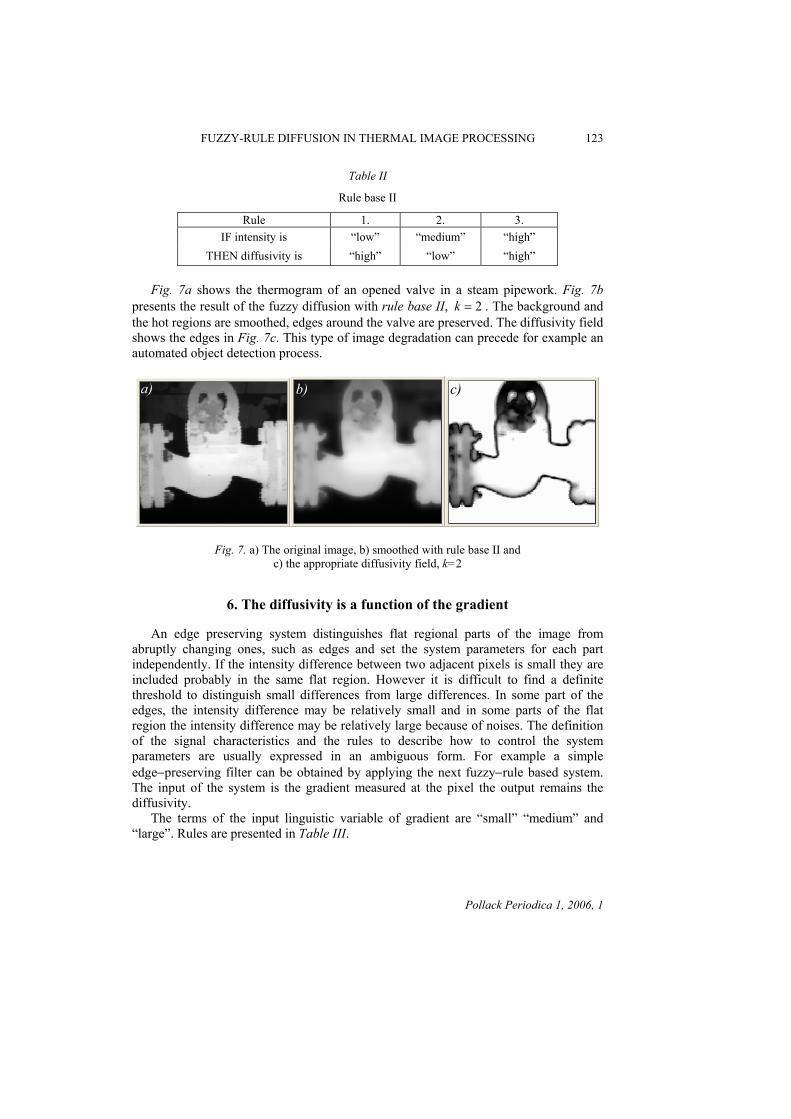
FUZZY-RULE DIFFUSION IN THERMAL IMAGE PROCESSING 123
Table II
Rule base II
Rule 1. 2. 3. IF intensity is “low” “medium” “high”
THEN diffusivity is “high” “low” “high”
Fig. 7a shows the thermogram of an opened valve in a steam pipework. Fig. 7b presents the result of the fuzzy diffusion with rule base II, 2=k . The background and the hot regions are smoothed, edges around the valve are preserved. The diffusivity field shows the edges in Fig. 7c. This type of image degradation can precede for example an automated object detection process.
a) c) b)
Fig. 7. a) The original image, b) smoothed with rule base II and c) the appropriate diffusivity field, k=2
6. The diffusivity is a function of the gradient
An edge preserving system distinguishes flat regional parts of the image from abruptly changing ones, such as edges and set the system parameters for each part independently. If the intensity difference between two adjacent pixels is small they are included probably in the same flat region. However it is difficult to find a definite threshold to distinguish small differences from large differences. In some part of the edges, the intensity difference may be relatively small and in some parts of the flat region the intensity difference may be relatively large because of noises. The definition of the signal characteristics and the rules to describe how to control the system parameters are usually expressed in an ambiguous form. For example a simple edge−preserving filter can be obtained by applying the next fuzzy−rule based system. The input of the system is the gradient measured at the pixel the output remains the diffusivity. The terms of the input linguistic variable of gradient are “small” “medium” and “large”. Rules are presented in Table III.
Pollack Periodica 1, 2006, 1

124 I. JANCSKAR, A. IVANYI
Table III
Rule base III
Rule 1. 2. 3. IF gradient is “small” “medium” “large”
THEN diffusivity is “high” “medium” “low”
The crisp value of the gradient is calculated from the neighboring pixel differences,
( ) max ,, mjkiijij IIg −−−= , 1 ,1, −=mk , 2,,1 −= ni L , 2,,1 −= nj L . (9)
The membership functions of the terms and the I/O characteristic of the system are shown in Fig. 8. The membership functions of the input terms are overlapped, so the transition from low to high diffusivity is continuous.
0
“low
”“m
ediu
m”
“hig
h”µ 1 0
Gradient
Diff
usiv
ity
“small”“medium” “large”µ1
Fig. 8. The I/O characteristic of an edge preserving system with rule base III
The IR−image of a closed steam−valve can be seen in Fig. 9a. The initial diffusivity field is shown in Fig. 9b. Contours of fine details are recognizable. The result of the diffusion process is shown in Fig. 10a, 3=k . Only the main edges remained in the corresponding diffusivity field, see Fig. 10b. Thought the fuzzy system has found the edges but not the same certainty. Diffusion passes through edges of higher diffusivity, consequently edges of lower diffusivity could be better retained. The presented edge−preserving filter has to be adapted to the processed images.
7. The diffusivity depends on the intensity and the gradient
The above−mentioned fuzzy systems determine their outputs from one input condition, from the intensity or from the gradient. If both conditions have to be considered, a fuzzy system with two input variable can be constructed, with and
Pollack Periodica 1, 2006, 1

FUZZY-RULE DIFFUSION IN THERMAL IMAGE PROCESSING 125
relationship between the terms. The rule base consists of 9 rules and can be written in a matrix form, see Table IV. Consequences are the elements of the matrix. Fig. 11 shows the characteristic of the constructed system in 3D. The fuzzy decision process with two activated rules is represented in Fig. 12.
b) a)
Fig. 9. a) The original image, b) the initial diffusivity field
Fig. 10. a) The filtered image and b) the corresponding diffusivity, after two smoothing sweep with the system of rule base III
Table IV
Rule base IV
Intensity Gradient “low” “medium” “high”
“small” “high” “low” “medium” “medium” “medium” “low” “medium”
“large” “low” “low” “low”
a) b)
When the rule has two antecedents, the activity index can be calculated with some of the fuzzy intersection operators [12]. In the presented examples and conjunction is supposed and the activity index is calculated by the min operator.
Pollack Periodica 1, 2006, 1

126 I. JANCSKAR, A. IVANYI
Fig. 11. I/O characteristic of the fuzzy system with two inputs and one output with rule base IV
Smoothing the original image in Fig. 9a with the system of rule base IV, the processed image and the diffusivity are shown in Fig. 13. The diffusivity field can be applied to detect the state of the valve. The average temperatures of the hot and cold valve regions can be easier evaluated from the smoothed image than from the original.
1. IF Intensity is “low” and Gradient is “small” THEN Diffusivity is “high”m
ax
Intensity
Diffusivity
“low” “medium” “high”
Crisp value
µ1
0 1
1
0 1
0
µ “low” “medium” “high”
“medium” “high”1
0 10
“medium”“large”
µ1
00 1
“small”
2. IF Intensity is “low” and Gradient is “medium” THEN Diffusivity is “ medium”
Intensity
“low” “medium” “high”
Crisp value
µ1
0 10
“medium” “high”1
0 10
“medium”“large”
µ1
00 1
“small” “low”
“low”min
β1
β2
Gradient
Gradient
Diffusivity
Diffusivity
min
min
Crisp value
Crisp value
Crisp value
Fig. 12. Graphical representation of fuzzy system operation with two inputs − one output
Pollack Periodica 1, 2006, 1

FUZZY-RULE DIFFUSION IN THERMAL IMAGE PROCESSING 127
Working with same linguistic variables and membership functions but modifying the rule base according to the rule base V in Table V, the brightest region can be retained and the other areas can be smoothed without blurring edges. The diffusivity function of the system is shown in Fig. 14. Result of the diffusion process and the diffusivity field can be seen in Fig. 15a and Fig. 15b, respectively.
Fig. 13. The image in Fig. 9a is filtered with the rule base IV a) result of diffusion, b) the diffusivity field, k=3
Table V
Rule base V
Intensity Gradient “low” “medium” “high”
“small” “high” “high” “low” “medium” “medium” “medium” “low”
“large” “low” “low” “low”
a) b)
Fig. 14. The I/O characteristic of the fuzzy system of rule base V
Pollack Periodica 1, 2006, 1

128 I. JANCSKAR, A. IVANYI
a) b)
Fig. 15.a) Image in Fig. 9a has been smoothed with the rule base V, b) the diffusivity field, k=3
Image details in the regions of highest intensities are retained. Because the low intensity of the edges, the intensities in the other areas have been smoothed only intra−regionally, i.e. temperature variations only in bounded regions have been attenuated, averaged. This type of image enhancing can be useful for better visualization and for automated supervising of equipments.
8. Conclusions
The fuzzy−rule based system is a new technique for the composition of the diffusivity function. The non−linear diffusion can be a very useful pre−processing technique in the enhancement of thermal images. The main advantage of the proposed image processing technique is its ability to handle the human’s conceptions in form of linguistic rules. It is easy expanded and formed to the user demands. Development of a system to an actual series of images, for example for computer vision, or to other engineering applications must be an iterative process that is based on the expert knowledge. The smoothing effect can be influenced by the number of the terms, by the shapes and overlaps of the membership functions. Not only the filtered thermal image, but also the diffusivity field can be a basis of segmentation or object detection processes.
Acknowledgments The research work has been developed in the frame of the project No. GVOP−3.1.1.−2004−05−0125/3.0.
References [1] Aubert G, Kornprobst P. Mathematical problems in image processing, Springer, New York,
2002. [2] Acton S.T. Multigrid anisotropic diffusion, IEEE Transactions on Image Processing,
Vol. 7, No. 3, 1998, pp. 280−291. [3] Catté F., Lions P.L., Morel J.M., Coil T. Image selective smoothing and edge detection by
nonlinear diffusion, SIAMJ. Numer. Anal. Vol. 29, 1992, pp. 182−193. [4] Weickert J. Anisotropic diffusion in image processing, Teubner, Stuttgart, 1998.
Pollack Periodica 1, 2006, 1

FUZZY-RULE DIFFUSION IN THERMAL IMAGE PROCESSING 129
[5] Barash D. Nonlinear diffusion filtering on extended neighborhood, Applied Numerical Mathematics, Vol. 52, 2005, pp.1−11.
[6] Polzehl J., Spokoiny V. Structural adaptive smoothing by propagation−separation methods, Weierstrass Institut für Angewandte Analysis and Stochastik, No. 1068, Berlin, 2005.
[7] Maldague X. Theory and practice of infrared technology for nondestructive testing, J. Wiley, New York, 2001.
[8] Tizthoosh H. R. Fuzzy−Bildverarbeitung, Springer, Berlin, 1998. [9] Chi Z., Yan H., Pham T. Fuzzy algorithms: With Application to image processing and pattern
recognition, World Scientific, Singapore, New Jersey, London, Hon Kong, 1998. [10] Arakawa K. Fuzzy rule based image processing with optimization, in Kerre E.E., Nachtegael
M. (Ed.) Fuzzy techniques in image processin, Physica−Verlag, Heidelberg, New York, 2000. [11] Perona P., Malik J. Scale−space and edge detection using anisotropic diffusion, IEEE
Trans. Pattern Anal. Machine Intell. Vol. 12, 1990, pp. 629–639. [12] Hollander I., Bajla I. Adaptive smoothing of MR brain images by 3D geometry−driven
diffusion, Computer Methods and Programs in Biomedicine, Vol. 55, 1998, pp. 157–176. [13] Jancskar I., Ivanyi A. Non−linear multigrid diffusion in thermal image processing, 12th
International Symposium on Interdisciplinary Electromagnetic, Mechanic & Biomedical Problems, Bad Gastein, Austria, 12−14 Sept. 2005, p.186.
[14] Jancskar I, Ivanyi A. Preisach Hysteresis Model for Non−linear 2D Heat Diffusion, Physica B, vol. 372, 2006, pp. 222−225.
[15] Kahlert J, Frank H. Fuzzy−Logik und Fuzzy−Control, Vieweg, Brunschweig/Wiesbaden, 1994.
Pollack Periodica 1, 2006, 1