Embed Size (px)
Citation preview

Durability of Adhesively-Bonded
CFRP/Steel Joints
Modelling of moisture ingress and joint degradation
Master’s Thesis in the Master’s Programme Structural Engineering and Building
Technology
LUIS DURAN JOFRE
ELOY OLAGÜE JULIÁN
Department of Civil and Environmental Engineering
Division of Structural Engineering
Steel and Timber Structures
CHALMERS UNIVERSITY OF TECHNOLOGY
Göteborg, Sweden 2013
Master’s Thesis 2013:123

I
MASTER’S THESIS 2013:123
Durability of Adhesively-Bonded
CFRP/Steel Joints
Modelling of moisture ingress and joint degradation
Master’s Thesis in the Master’s Programme Structural Engineering and Building
Technology
LUIS DURAN JOFRE
ELOY OLAGÜE JULIÁN
Department of Civil and Environmental Engineering
Division of Structural Engineering
Steel and Timber Structures
CHALMERS UNIVERSITY OF TECHNOLOGY
Göteborg, Sweden 2013

II
Durability of Adhesively-Bonded CFRP/Steel Joints
Modelling of moisture ingress and joint degradation
Master’s Thesis in the Master’s Programme Structural Engineering and Building
Technology
LUIS DURAN JOFRE
ELOY OLAGÜE JULIÁN
© LUIS DURAN JOFRE, ELOY OLAGÜE JULIÁN, 2013
Examensarbete / Institutionen för bygg- och miljöteknik,
Chalmers tekniska högskola 2013:123
Department of Civil and Environmental Engineering
Division of Structural Engineering
Steel and Timber Structures
Chalmers University of Technology
SE-412 96 Göteborg
Sweden
Telephone: + 46 (0)31-772 1000
Cover:
The configuration of the studied double-lap-shear joint on top, and on the bottom
moisture diffusion progress and degradation of the joint as a function of time
Chalmers Reproservice
Göteborg, Sweden

III
Modelling of moisture ingress and joint degradation
Master’s Thesis in the Master’s Programme Structural Engineering and Building
Technology
LUIS DURAN JOFRE
ELOY OLAGÜE JULIÁN
Department of Civil and Environmental Engineering
Division of Structural Engineering
Steel and Timber Structures
Chalmers University of Technology
ABSTRACT
The aim of this study is to model the moisture diffusion and consequently degradation
of an adhesively bonded CFRP/steel joint. Different failure modes and diffusion
models are investigated, while joint strength degradation with respect to time and
exposure is presented. The damage mechanic approach Cohesive Zone Modelling
(CZM) is used as a method to describe the adhesive joints strength, the commercial
Finite Element Method (FEM) program ABAQUS is used as a tool to simulate and
compare the experimental test results. The main methodology of this work consists in
using results from laboratory test that gives the traction-separation laws of the
adhesive and then apply these parameters to simulate other tests to verify the
independency of the models performed in ABAQUS. The tests that are used to get the
traction-separation laws and the test that are used to verify the models are strictly
independent from each other’s. The only relation that exists between them is the type
of adhesive and the mechanical behaviour of the joints. The tests that are used to
identify the traction-separation law of the adhesive in question are the DCB, ENF and
MCB-test. The test that are simulated and also used to verify the models in ABAQUS
are the DLS and RTB-test. However, the aim in this work is to predict the joint
strength degradation and this is performed in ABAQUS. ABAQUS has been showed
to be able to easily perform diffusion analysis by using the well-known analogy and
cross-coupling between the heat conduction and moisture diffusion. The moisture
profile used in this work is verified by Fick’s second law calculations performed in
MATLAB. Specifically, the cohesive zone modelling has been used and the
respective moisture dependent traction-separation law of the adhesive have
conceptually been modelled in ABAQUS. The moisture dependent traction-separation
law for the different modes are formulated and described.
Key words: Adhesive, damage mechanics, cohesive zone modelling, CZM,
moisture dependent, MMF, gravimetric test, moisture dependent, traction-separation
law, ABAQUS, numerical method, continuum mechanics, fracture mechanics, epoxy,
failure mode, mode I, mode II, mixed mode.

CHALMERS, Civil and Environmental Engineering, Master’s Thesis 2013:123 IV

CHALMERS Civil and Environmental Engineering, Master’s Thesis 2013:123 V
Contents
ABSTRACT III
CONTENTS V
PREFACE VII
NOTATIONS VIII
1 INTRODUCTION 1
1.1 Aim and Objectives 1
1.2 Method 1
1.3 Limitations 2
1.4 Outline of the Thesis 3
2 LITERATURE STUDY 5
2.1 Materials 5
2.1.1 Carbon Fibre Reinforced Polymer (CFRP) 5 2.1.2 Steel 5 2.1.3 Structural Adhesives 5
2.1.4 Adhesives Bonding 6
2.2 Numerical Modelling of Adhesive Joints 8 2.2.1 Finite Element Method 8 2.2.2 Boundary Element Method 10
2.2.3 Finite Difference Method 10 2.2.4 Numerical method selection 10
2.3 Mechanical Modelling Approaches 12 2.3.1 Continuum Mechanics 12 2.3.2 Fracture Mechanics 14 2.3.3 Damage Mechanics 16
2.3.4 Mechanical method selection 17
3 COHESIVE ZONE MODELING 19
3.1 The traction-separation law: 20
3.1 Traction-separation for pure Mode I 21
3.2 Traction-separation for pure Mode II 23
3.3 Mixed Mode (Mode I and Mode II) 25
4 MODELING OF MOISTURE DISTRIBUTIONS IN ADHESIVE JOINTS 29
4.1 Theory background 29 4.1.1 Fickan model 29
4.1.2 Two dimensional equation 31 4.1.3 Different mass uptake equations 31
4.2 Experimental test and results 33

CHALMERS, Civil and Environmental Engineering, Master’s Thesis 2013:123 VI
4.2.1 Gravimetric test 33 4.2.2 Gravimetric test results 33
4.3 Verification of our model 34 4.3.1 Finite element method and analytical method 34
4.3.2 Analogy between heat and moisture 34
5 EXPERIMENTS 37
5.1 DCB-test results 39
5.2 ENF-test results 40
5.3 MCB-test results 41
5.4 TRB-test 46
5.5 DLS test 48
6 FINITE ELEMENT MODELING AND ANALYSIS 53
6.1 Material properties 53
6.2 CZM parameters 53
6.3 TRB-joint simulation 54
6.3.1 Description of the models 54
6.4 DLS-joint simulation 58
6.4.1 Description of the 2D models 58 6.4.2 Description of the 3D model 75
6.5 Coupled analysis 78 6.5.1 Influence of moisture in the adhesive properties 78 6.5.2 Simulation of wet DLS-test 78
7 RESULTS AND FURTHER INVESTIGATION 81
7.1 Corrosion 81
7.1.1 FTIR test 81
7.2 Quantify the degradation of the adhesive 81
8 CONCLUSION 82
9 REFERENCES 83
APPENDIX A A

CHALMERS Civil and Environmental Engineering, Master’s Thesis 2013:123 VII
Preface
This study is a part of a research project concerning mechanical properties and
durability of adhesive bonds in CFRP/steel joints. The project is carried out at the
Department of Structural Engineering, Timber and Steel Structures at Chalmers
University of Technology, Sweden from January 2013 to July 2013.
We would like to express our deep gratitude to our supervisor, Mohsen Heshmati, for
his guidance, support, and inspiring collaboration. This study could have never been
conducted without the sense of high quality and professionalism of him.
Göteborg July 2013

CHALMERS, Civil and Environmental Engineering, Master’s Thesis 2013:123 VIII
Notations
J: Energy release rate
Jc: Critical energy release rate
E: Young modulus
K: Stress intensity factor
Kc: Fracture toughness
Tn,max: Traction stress in normal direction (Damage initiation)
Ts,max: Traction stress in shear direction (Damage intiation)
Tn,mix: Damage initiation in normal direction in Mix-mode
Ts,mix: Damage initiation in shear direction in Mix-mode
wc: Critical displacement in normal direction
vc: Critical displacement in shear direction
δc: Mix-mode critical displacement
τ: Shear stress
σ: Normal stress
τ0: Damage initiation
σ0: Damage initiation
D: Damage parameter
F: Applied force
θA: Rotational angle
εs: Swelling strain
CME: Coefficient of moisture expansion
∆Mt: Moisture uptake

CHALMERS Civil and Environmental Engineering, Master’s Thesis 2013:123 1
1 Introduction
A large number of steel bridges all over the world need to be repaired or upgraded.
There are many bridges that are experiencing advanced levels of deterioration because
of the environmental exposure during their service life. The upgrading of old bridges
can be motivated by the need for them to be able to take higher load because the
transportations vehicles are increasing in both size and load [1].
The rehabilitation of steel bridges using advanced composite materials offers the
possibility of a short-term retrofit or long-term solution for bridge owners faced with
deficient structures. The high strength-to-weight ratios along with corrosion resistance
are appealing factors in favour of the use of Carbon Fibre Reinforced Polymer
(CFRP) as a strengthening method of steel structures. The ease of application, if
comparing with applying a welded steel plate, introduces cost savings associated with
labour, time, and inconvenient to public transportation [2]. In other words, is a social
economical alternative for the repair or upgrade of steel bridges that are currently in
service [1].
CFRP has shown some unique advantages among other construction materials such as
excellent resistance to corrosion and environmental degradation, high longitudinal
strength, high fatigue endurance and reduced weight. These features have made the
CFRP adequate for reinforcing structures that are being affected by degradation.
Adhesive bonding as a joining technology consist basically of taking a strip of, for
example CFRP, and gluing it to the material that need to be reinforced. This easy
procedure have as mentioned earlier many advantages in comparison with other
joining technics as, for example, welding and bolting. Nevertheless the adhesive
material is the weakest link in this joint system when looking at the long-time
performance of adhesive joints [1, 2].
The durability of these bonded joints still remains as a disadvantage when the
engineer has to take decisions about witch joining technology to use, mainly because
of the lack of knowledge concerning the durability of these joints. The lack of long-
term and high initial costs is characterised issues of new materials when the
technology is relatively new. In this study, the durability issue is investigated with
focus on the moisture ingress in bonded joints and how it affects the strength of the
joint through its service life [1].
1.1 Aim and Objectives
The aim of this thesis is to predict the failure strength and durability of CFRP/steel
joints. The objective is to research the use of CFRP strengthened steel in bridge
structures and presents a methodology that can predict the failure load of statically
loaded aged and un-aged adhesive joints.
1.2 Method
To realise the objectives of this thesis a literature study about the “state-of-the-art”
concerning the mechanical behavior and durability of CFRP/steel joints is performed.
A mechanical and numerical approach is chosen based on the literature study. The
moisture diffusion of the adhesive and the degradation of an adhesively bonded
CFRP/steel joint strength due to moisture concentration is identified and modelled.
The mechanical method used consists of performing test that describes the damage

CHALMERS, Civil and Environmental Engineering, Master’s Thesis 2013:123 2
initiation, this is a relation between deformation and strength behaviour of the
material, and also gives an energy parameter that describes the damage propagation.
This damage initiation and damage propagation is in this work called the traction-
separation law of the material. The tests that are used in this work to identify the
traction-separation laws of the adhesive used are the DCB, ENF, and MCB-test. Once
well obtained the traction-separation laws it is possible to simulate and predict the
behaviour of aged and un-aged adhesively bonded specimens. The tests that are used
to verify the models are the TRB and DLS-test. The mechanical theory used is the
Cohesive Zone modelling (CZM) and the numerical method is the finite element
commercial program ABAQUS.
1.3 Limitations
Due to the size of this thesis, concerning time and resources, some approaches are
going to be taken.
The degradation rate are assumed and described in chapter 6.5.
The interfacial degradation do to wander walls forces and corrosion formation is
ignored. Interfacial moisture diffusion is also left out.
Diffusion model is restricted to Fick´s second law.
Temperature over the glass transition, cyclic loads, cyclic temperature and water
exposure are all ignored.
Literature study
Diffusion Theory
Analytical and numerical
Gravimetric test
Diffusion analysis with
ABAQUS
Simulation of aged samples
Identifying the methodology
Mechanical and numerical
CZM and ABAQUS
The traction-separation
laws
Prediction of un-aged
sample test
Coupled analysis
Figure 1 Work Method

CHALMERS Civil and Environmental Engineering, Master’s Thesis 2013:123 3
1.4 Outline of the Thesis
Figure 2 Outline of the thesis
Theory and methods used (Chapter 3-4)
Initial steps (Chapter 2)
Test and simulations
(Chapter 4-6)
Litera
ture
stud
y
Diffusion theory Ficks law
Simulation verify
analyticaly
Mechanical and numerical approaches
Cohesive Zone Modeling
(CZM)
Test to obtain the traction-
sepration law
Finite Element Method
(ABAQUS)
Simulation of test.

CHALMERS, Civil and Environmental Engineering, Master’s Thesis 2013:123 4

CHALMERS Civil and Environmental Engineering, Master’s Thesis 2013:123 5
2 Literature study
2.1 Materials
2.1.1 Carbon Fibre Reinforced Polymer (CFRP)
The Encyclopaedia[3] defines CFRP as:
“Carbon fibre reinforced Plastic (CFRP) is a strong and light composite material or
fibre reinforced polymer. Like glass-reinforced plastic, the composite material is
commonly referred to by the name of its reinforcing fibres (carbon fibre). The
polymer is most often epoxy, but others plastics, like polyester or vinyl ester, are also
sometimes used”.
In the context of durability of the CFRP/steel joints, the durability of the CFRP is not
the critical point in these joints, because it has shown excellent resistance against
hostile environmental exposure in strengthening systems [4-6]. Due to this evidence,
the investigation is focusing on the durability of the adhesive between these two
materials (steel and CFRP) [7].
2.1.2 Steel
The steel that is used in this work is a S355 structural steel with high strength and low
alloy, is a European standard structural steel EN 10025-2004 standard. The typical
applications of the S355 steel include:
Bridge components, components of offshore structures
Power plants
Wind tower components
Mining and earth moving equipment.
2.1.3 Structural Adhesives
R.D. Adams defines in his book (Structural Adhesive Joints in Engineering, R.D.
Adams, J. Comyn, W.C. Wake – 1997) the term adhesive as a polymeric material that,
when applied to an adherent surface, e.g. a metal adherent or a CFRP material, can
join them together and resist separation [8].
In this study, the adhesive used is StoBPE lim 567. It is a two-component, solvent-
free structural epoxy adhesive. According to the producer, after a week of curing the
adhesive has the following characteristics:
Table 1 Material properties of StoBPE lim 567
E-modulus: 7 GPa
Poisson´s ratio: 0.3
Tensile strength: 26 MPa
Strain to: failure 0.82 %

CHALMERS, Civil and Environmental Engineering, Master’s Thesis 2013:123 6
2.1.4 Adhesives Bonding
Although adhesive joints have important advantages against mechanical joint, e.g.
lower structural weight, lower fabrication cost, and improved damage tolerance [9],
all adhesives are, to some degree, permeable to water or moisture ingression. The
moisture ingression changes with temperature, interfacial strength degradation and
bulk properties are all factors that affect the durability of adhesive joints. For these
reasons the adhesive material is the weakest link in these joint[10-12].
The moisture is able to change the bulk material properties of the adhesive, e.g. the
glass transition temperature, modulus and tensile strength [13]. Different types of
adhesives have different diffusion coefficients and moisture influences. This means
that the rate of changes, e.g. plasticisation rate of the adhesive due to diffusion varies
among the different types of adhesives [14].
Moisture can also act at the interface of the adherent/adhesive joint. When the water
molecules are absorbed into the adhesive the moisture transport is concentrated on the
metal adherent and this accumulation of water at the interface accelerate the
displacement of the adhesive from the metal surface [13]. The appearance of
corrosion at the interface of the metallic adherent is also a reason of higher
degradation rate of the interface strength [15, 16]. Measures taken in experiments
have shown that the loss of strength and stiffness of CFRP/steel are likely due to loss
of cross-sectional area which can be represented by the mass loss because of
corrosion, and not by degradation of material properties [5].
Pocius and co-workers [17] study showed that there is a critical combination of
temperature, humidity and load that produce rapid loss of the adhesive joint strength.
They also showed that the durability of steel joints and aluminium joints have an
interesting behaviour. The experimental study performed by them showed that the dry
lap-shear strengths are similar for both steel and aluminium, however a total different
behaviour was found for water exposed lap-shear joints. In lap-shear joints exposed to
a humid environment, joint with steel adherent fail after 30 days while the ones with
aluminium adherent fail after around 3000 days.
In summary, two main effects that can reduce the strength of CFRP/steel adhesive
joints can be identified.
The properties of the bulk adhesive
The adhesion properties at the interface
It has been mentioned that a strength recovery of the joints is observed after
desorption of moisture [14] . Analysis done in [14] of the failure surfaces revealed
that the dry joints failed cohesively in the adhesive layer and that the failure path
moved towards the interface after conditioning. The failure mode then reverted back
to cohesive failure after moisture desorption. Although, these results are not general
for all types of adhesives, the adhesive material does have some recovery properties in
some cases.
The properties of the adhesive are strongly dependent of its composition. This means
that to change the moisture resistance or the mechanical behaviour the formulator
generally must operate on the bulk adhesive. This will occur mainly through
modification or change in the bulk polymer and somehow by modification or change
of the fillers and additives in the formulation[18].

CHALMERS Civil and Environmental Engineering, Master’s Thesis 2013:123 7
When studying the mechanical behaviour of the adhesive joints it is commonly to
divide the deformation directions of the joint in mode I, mode II and mode III, shown
in Figure 3. Mode I being an opening mode of the crack region and is in direct
relation to the normal stresses of the crack surface. The mode II is the sliding mode
and is in relation to the shear stresses in the crack surface area. Mode III is the same
as mode II but mode III being in the respective shear and sliding mode of the second
direction of the local coordinate system.
Figure 3 Deformation modes
Independent of the opening mode of the crack region there is a division of the failure
mode of the adhesive joint. When the failure is in the adhesive layer it is called
cohesive failure and, in the other hand, when the failure is in the transition zone
between the material, from adherent to adhesive, then it is called interfacial failure,
Figure 4.
a) b)
Figure 4 Failure modes. a) Cohesive failure and b) Interfacial failure
To correctly predict and describe the behaviour of the failure models and paths it is
first necessary to decide and choose a mechanical and numerical method. Various
mechanical and numerical methods have been applied in adhesive joints and the
history and developing of the predictive tools have been well summarised by the work
of Da Silva[9, 19]. The chapter 2.2 true out 2.3 describe the work of Da Silvia that is a
satisfactory “state-of-the-art” of the history of mechanical and numerical methods that
have been used for adhesive joints, from the begging of adhesive joint theory to the
modern trends and methodology’s.

CHALMERS, Civil and Environmental Engineering, Master’s Thesis 2013:123 8
2.2 Numerical Modelling of Adhesive Joints
In [9] Silvia explains the tree numerical methods used to solve differential equations,
Finite Element Method (FEM), Boundary Element Method (BEM) and Finite
Difference Method (FDM). The work of Silvia is a very interesting “state of the art”
of the different numerical methods and gives examples of how the methods are
applied to adhesive joints in modern research. All the different numerical methods are
described, and examples are given where they are most adapted to be applied.
Because there is no perfect theory nowadays that is capable of solving any given
problem concerning adhesive joints, the engineer has to be aware of the limitations in
each one of the numerical methods [9, 20].
2.2.1 Finite Element Method
The Finite Element Method (FEM) is a numerical analysis procedure that provides an
approximate solution. There exist a grand variety of commercial FE analysis
programs today and they have the possibility of performing coupling analysis, such as
e.g. hydro-thermo-structural problems, and this method is also suitable for complex
geometries [9]. To model the joint strength the analyser needs to have the stress
distribution and a suitable failure criterion. The stress distribution can be obtained by
FE analysis or a closed-form model. There are numerous amounts of approaches for
the FEM and the failure criterion. The simplest failure model is the stress, strain or
energy limits and it is one of the commonly used in continuum mechanics approaches.
The fracture mechanics principal can also be modelled by commercial FEM
programs. This can be based on the stress intensity factor approach or the energy
release rate approach and finally the damage mechanics that is the combination of the
continuum mechanics approach and the fracture mechanic [9] with both damage
initiation criteria and propagation criteria, as for example the Cohesive Zone
Modelling (CZM).
FEM is basically the discretization of a structure in various sub domains called
elements that are joined at their nodes. Each node has a given number of Degree of
Freedom (DoF). Now the structure, that is a continuum, is represented by nodes with
degrees of freedom. In elasticity problems the solutions for the equilibrium equations
is to solve the governing partial differential equation. The variation method is one
way of finding approximations and is used in FEM to solve the elasticity differential
equation by determining the condition that makes a functional stationary. A functional
is a function of another function and in elasticity problems the functional used is the
potential energy of the structure. Taking into account internal compatibility and
essential boundary conditions, optimal values are searched and those are the ones that
minimise the total energy. This process of minimisation gives a system of equations
for the field quantity of the nodes and can be described by the Eq. 1.
Eq. 1
Where delta is a vector with the field values, K is the stiffness matrix and F a vector
with the loads on the structure. There are integrals in the stiffness matrix K that may
be needed to be solved with a numerical integration scheme. Generally, the integral
can be computed by using gauss points and multiplying with factors with appropriate
values. However, these elements can be made by drawing continuum lines between
the nodes and thereby creating a mesh in the structure. The mesh sizes govern the
accuracy of the stress gradients over the structure represented by the nodes. Because,

CHALMERS Civil and Environmental Engineering, Master’s Thesis 2013:123 9
if we have more nodes we also have more elements and that means a finer mesh. In
other words, more nodes mean more information about what is going on in the
structure. Nevertheless, in adhesive joints there are stress singularities at the ends and
the mesh refinement can lead the stresses to infinity. These convergence problems can
be avoided by using a correct approach e.g. elasto-plastic and fracture mechanics
concepts.
Figure 5 Mesh intensity
The commercial FE programs permit to choose the material model to determine the
initial yielding and subsequent plastic deformation in a bonded joint. For the metal
adherent the Von Mises yield criterion may be applied and, for the adhesive, a
yielding model that takes into account the hydrostatic pressure is generally required.
Raghava describe in his work [21] the yielding criteria for polymers that is a version
of the Von Mises criterion. This criterion takes into account the differences between
tensile and compressive yield strengths and considers any dependence of yielding on
the hydrostatic component of the applied stress state. In ABAQUS there exist pre-
defined options to use, as for example the Cohesive Zone Model (CZM) that is based
on Damage mechanics. The CZM is explained in the Chapter 2.3.3. To use the CZM it
is necessary to obtain traction-separation law or cohesive laws. That is the relation
between the forces that work against separation and the displacement in a crack or at
the interface of an adhesive joint. The form of these traction-separation laws can be
defined differently and there exist many different approaches to use to obtain them.
However, it is always needed to first establish the initiation and the propagation
criterion of the separation rate and this is possible to achieve in the commercial FEM
programs, as for example ABAQUS. The traction-separation laws are found by
experiments. The use of moisture dependent traction-separation laws need in normal
cases a great amount of tests before it is possible to do accurate simulations of the
long-time performance of the adhesively bonded joints.

CHALMERS, Civil and Environmental Engineering, Master’s Thesis 2013:123 10
2.2.2 Boundary Element Method
The Boundary Element Method (BEM) is a typically used numerical method in
engineering applications and it has been proved to be useful when dealing with
fracture mechanics. In FEM the stresses are evaluated inside de elements and in BEM
the stresses are evaluated at the boundaries, e.g. at the crack boundary. This
representation of stress distribution has been shown to give a good resolution of the
stress gradient in the thickness direction of an adhesive joint. Unfortunately, when
the stress gradients are along the boundary, as for the interface, then the BEM, like the
FEM, requires a refined mesh and the BEM needs to have specialized infinitive
boundary element to properly model the interfacial behavior [9].
In the work of Vable [22] the author explain that BE-method can be used effectively
in stress analysis of adhesive joints. The result in Vable’s work showed that BEM is
able to perform parametric study of the joint parameters, such as optimization of
mesh. The paper demonstrates the easy way of modeling changes in geometry, e.g.
different spew angels. It is also discussed that if a similar stress concentration curves
existed for adhesive joint as it exist for design of mechanical fastened joints, the BEM
can well become a methodology of choice for stress analysis of adhesively bonded
joints.
2.2.3 Finite Difference Method
The Finite Difference Method (FDM) is a numerical technique for approximating the
solutions to differential equations, by using finite difference equations to approximate
derivatives. Differential equations are well used in both the diffusion analysis and the
different types of beam theory approaches used in adhesive joint analysis. So this
numerical method is definitely an alternative for the study of durability of adhesively
bonded joints.
In the work of Silvia [9] the FDM is discussed and the mayor advantage is the simple
computer implementation. Therefore this method is easily used when creating codes
and new features are easy added. The main disadvantage is the boundary conditions
for complex geometry’s and problems with the stiffness matrix, and therefore this
method have most been used for simple geometries [23].
2.2.4 Numerical method selection
Although all numerical methods are to some degree applicable to adhesive joints
analysis the method in this work is going to be FEM. The main reasons are presented
in Table 2. The easy of performing both diffusion analysis and moisture dependent
traction-separation laws in ABAQUS is a strong reason for choosing FEM. Another
reason is that when performing the literature study of adhesive joint analysis, FEM
seem to be the main numerical method used in current research.

CHALMERS Civil and Environmental Engineering, Master’s Thesis 2013:123 11
Table 2 Pros and cons of different numerical methods concerning adhesive joints.
Finite Element Method
Pros:
Commercial program with predefined options
for adhesive joints analysis.
Numerous amounts of approaches for the
failure criterion.
Coupled analysis is easy to use in ABAQUS
(moisture dependent traction-separation laws)
Diffusion analysis by the analogy of heat
analysis (ABAQUS).
Cons:
Finer mesh takes longer time
ABAQUS traction-separation laws differs
from many other traction-separation forms
presented in other literature
Subroutines are not as straight forward to use
as the predefined options.
Boundary Element Method
Pros:
Give a good resolution of the stress gradient in
the thickness direction of an adhesive join
Useful in fracture mechanics
Useful for performing parametric study
Cons:
Need infinity boundary when analyzing
interfacial adhesive joint strength
Not enough rehearse performed with this
numerical method
Finite Difference Method
Pros:
Can be used for diffusion analysis
Can be used to solve beam-theory used in
adhesive joint analysis
Cons:
Do not work for complex geometries
Not enough research performed with this
numerical method

CHALMERS, Civil and Environmental Engineering, Master’s Thesis 2013:123 12
2.3 Mechanical Modelling Approaches
2.3.1 Continuum Mechanics
A simplified explanation of the continuum mechanics approach consists on comparing
the maximum stress, strain or strain energy with the material allowable ones and,
thereby, obtaining a failure criterion. Continuum mechanics is one of the simplest
approaches to obtain a failure criterion and it can easily be used in the FE analysis [9].
2.3.1.1 Disadvantages and adaptation of continuum mechanics
The continuum mechanics approach has problems in the sharp corners, e.g. singularity
problems. This implies that the model is not accurate to model traditional adhesively
bonded configurations, as for example, Double Lap Shear joint (DLS-joint), Double
Cantilever Beam joint (DCB-joint), Mixed Mode Cantilever Beam joint (MCB-joint)
and Tensile Reinforced Bending joint (TRB-joint). Using the continuum mechanics
approach give a high mesh-dependency. However, rounding of the sharp corners
removes the singularity and reduces the high values of stress, energy, and strain.
Strain criterion has been used to predict failure in some studies but the site of damage
initiation and propagation to failure in adhesive joints is highly dependent on the
geometry and the edges of the overlap [24].
The maximum stress, strain and energy failure mode has been successively used to
predict joint strength with some types of brittle adhesive and with short overlaps. On
the other hand, in continuum mechanics it’s not appropriate to use a criteria based on
stresses when a ductile adhesive is used [9].
The stress, strain and energy failure criterion are all applicable to continuum structure
only, and therefore have difficulties when defects are presented or more than one
material is analysed. Because continuum mechanics assumes that structures and
materials are continuous, consequently e.g. defect in the form of cracks or sharp
corners are not properly analysed since discontinuities that gives convergence
problem arises in those spots. The problem with the continuum mechanics is in the
zone that is cracked, the free surface is absence from stresses and the zone near the
crack has the highest stresses, consequently discontinuities and convergence appears.
This problem is also presented in bonded joints of two materials with a re-entrant
corner, but here only the stress discontinuities exist and the free surface do not. More
generally, for the continuum mechanics it’s always exist discontinuities if the crack or
the material connection is smaller than 180 degrees [9].
2.3.1.2 To take into account before using continuum mechanics
The continuum mechanics approach take only into account the principal stresses in
the right direction of the external applied force of a single or double lap test and
ignores all the other stresses, e.g. normal stresses existing in the lap joints and
therefore overestimates the total joint strength [9]. In the other hand, Adams [25]
showed that Poisson’s ratio strains in the adherents of a simple adhesive lap joint
induce transverse stresses both in the adhesive and adherents. The work by Adams
describe that two simultaneous second-order partial-differential equations can be set
up to describe the normal stresses along and across an adherent and this equations cud
be solved both by an approximate analytical method and a Finite Difference Method
(FDM).

CHALMERS Civil and Environmental Engineering, Master’s Thesis 2013:123 13
The continuum mechanics is a straight forward approach and it does not need any
traction-separation parameters from experiments, as for the fracture and damage
mechanics. In the other hand, it’s important to be aware of the limitations as e.g. the
geometry, mechanical behavior and material dependency of the model.
Figure 6 Singularity at the crack tip
CHALMERS, Civil and Environmental Engineering, Master’s Thesis 2013:123 14
2.3.2 Fracture Mechanics
To model the ultimate carrying capacity and the structural integrity it is important to
take the discontinuities into account. This need of dealing with this important issues in
engineering have developed the fractural mechanics in the form of Linear Elastic
Fracture Mechanics (LEFM) to deal with the discontinuities and the Elastic-Plastic
Fracture Mechanics (EPFM) to deal with the formation and propagation of material
with plastic deformation [26]. The EPFM can also be called yielding fracture
mechanics (YFM).
Materials with low fracture resistance fail below their ultimate load and can be
analyzed on the basis of continuum mechanics concepts through the use of LEFM. If a
body with a crack is subjected to a loading mode I, the material will be considered
elastic, naturally following Hooke's law [27]. Fracture will occur when the stresses at
the crack tip become too high for the material. As the stress intensity factor (K)
determines the entire crack tip stress field. The fracture will occur when K becomes
too high for the material. How high the stress intensity is dependent of the material
chosen and it must be determined from experimental tests [27]. The material's fracture
toughness (Kc) can be recognized as the critical maximum stress intensity (K) which
the material can withstand without drastic crack propagation in the material.
In LEFM the crack tip behavior can be characterized by the stress intensity factor (K)
that describes the effect of loading at the crack tip region and the resistance of the
material and is valid for a small region around the crack tip. LEFM concepts are valid
if the plastic zone is much smaller than the singularity zones. In the other hand, in
EPFM the crack tip undergoes significant plasticity.
EPFM is applied to materials, generally, in the case of large-scale plastic deformation.
Three parameters are generally used: Crack opening displacement (COD) or crack tip
opening displacement (CTOD) and the well-used J-integral. These parameters give
geometry independent measure of fracture toughness
By idealizing elastic-plastic deformation as non-linear elastic the J-integral
characterizes the crack tip stress and crack tip strain and energy release rate. In LEFM
the cohesive zone is assumed small in comparing with the crack length. In this
approach, the external load can be represented by the stress intensity factor K or
energy realize rate J. the fracture toughness is the critical value for the stress intensity
factor
This approach does not take into account what is happening in the cohesive zone [28].
The main idea is that the crack propagation is determined by the relation between the
release of potential energy and the necessary surface energy to create new surface area
as the crack propagates. It was asserted that when a crack grows, the decrease of
potential energy is compensated by the increase of the surface energy caused by the
tension in the new cracked surface [29].
2.3.2.1 Disadvantages and adaptation of fracture mechanics
In LEFM parameters as, e.g. the Stress intensity factors are difficult to establish when
the crack grows at or near an interface. Instead the energy release rate, J, and the
critical energy release rate, Jc can be used. However, a strain singularity still exists for
ductile materials, even though the stress singularity has disappeared. Linear Elastic
Fracture Mechanics (LEFM) has been used to overcome singularity problems and can

CHALMERS Civil and Environmental Engineering, Master’s Thesis 2013:123 15
be used in different layouts of fillets for bonded joints, but the LEFM do not work
when the material have plastic deformation before failure. There exist modifications
of the approach but the all need a great amount of parameters to best fit the
experimental data[9].
The Elastic-Plastic Fracture Mechanics (EPFM) has been used to model plastic
behaviour introducing the J-integral that is used to predict the joint strength of cracked
adhesive joints satisfactory. The mayor disadvantage of the use of the J-integral to
model adhesive joints is that it’s dependent of the interfacial length and therefore the
J-integral have to be extrapolated to find the new values and a new mesh have to be
establish.
It have been shown that the EPFM need to have a predefined crack path and this
imply that the failure mode can be highly complex and doubtful some time [9].
2.3.2.2 To take into account before using fracture mechanics
In the cases where the global stress-strain response of the body is linear and elastic,
the use of LEFM is suitable and the stress intensity factor K is used. Many studies
dealing with adhesive joints use the strain energy release rate, J, and the critical value
of the energy release rate Jc, because is easier than to find the stress intensity factor K
and the Fracture toughness, Kc.
Figure 7 The stress intensity factor is defined from the elastic stress field equations
for a stressed element near the tip of a sharp crack under biaxial (or uniaxial) loading
in an infinite body.

CHALMERS, Civil and Environmental Engineering, Master’s Thesis 2013:123 16
2.3.3 Damage Mechanics
Damage mechanics is the study of material damage based on damages variables. This
damages variables changes with the applied load condition to quantitatively represent
the growth of mechanical deterioration of a material component. Structural damage
during loading can be found in the form of micro cracks over a finite volume or
interface region between bonded components. Damage mechanics permits the
simulation of step-by-step damage and fracture at an arbitrarily finite region, up to
complete structural failure [8, 9, 26, 27, 30-34].
There exist two main approaches available for damage modelling and they are the
local approach and the continuum approach. In the local approach, damage is
confined to a zero volume line or a surface, allowing the simulation of an interfacial
failure between materials, e.g. between the adhesive bond and the adherent. By the
continuum approach, the damage is modelled over a finite region, within solid finite
elements of structures to simulate a adhesive failure or along an adhesive strip to
model an interfacial failure of the adhesive joint. The Cohesive zone model (CZM)
can be used in both approaches (local and continuum) and it can simulate the
macroscopic damage along a path by the specification of a traction-separation
response between paired nodes on ether sides of a pre-defined crack path. The CZM
simulate the fracture process better than traditional fractural mechanics, by extending
the concept of continuum mechanics using both strength and energy parameters to
characterize the debonding process [9].
2.3.3.1 Disadvantages and Adaptation of Damage Mechanics
This method presents limitations because it is necessary to know beforehand the
critical zones where damage is prone to occur and a methodology is needed to
characterise the moisture-dependent cohesive zone properties in a satisfactory way.
A traction–separation response is used to model the damage initiation and evolution
in the fracture process zone (Cohesive Zone), and for ductile materials the shape of
traction-separation laws must be modified which can give convergence problems [9].
In the work of Katnam [31] characterisation of moisture-dependent cohesive zone
properties have been identify for a cohesive failure mode. It is also discussed there,
that the same approach can also be useful for an interfacial failure mode.
Consequently, the critical energies and tractions parameters are related to the
degraded interface traction-separation law, rather than the bulk adhesives properties as
for the adhesive failure.
In the work of Yang [35] a mode-dependent embedded-process-zone (EPZ) model has
been developed and it is used to simulate the mixed-mode fracture of plastically
deforming adhesive joints with Mode-I and Mode-II fracture parameters combined
with a mixed-mode failure criterion to run quantitative predictions of the deformation
and fracture of mixed-mode geometries. These numerical calculations have been
shown to provide excellent predictions for geometries that experience large-scale
plastic deformation such as single lap-shear joints. Details of the deformed shapes,
loads, displacements and crack propagation have all been well predicted by the
calculations.

CHALMERS Civil and Environmental Engineering, Master’s Thesis 2013:123 17
2.3.3.2 To take into account before using Damage Mechanics
When EPFM is used the fracture characterizing parameters are the J-integral or the
crack opening displacement (COD). All these fracture characterizing parameters meet
both the Griffith energy criterion and the critical stress/strain criterion. The three
modes, mode I, mode II and mix-mode of crack propagation are all associated with
the fracture energy concepts.
The fracture parameters may be chosen so the model best fits to the experimental data,
or they may be prescribed based on some assumed relationship. Fabricating such
models will require an increasing number of independent material parameters, which
must all be pre-obtained or re-adjusted by experiments. Apart from the amount of
experimental work involved, this purely mathematical fracture parameter fitting
method does not explain the physical failure mechanism [36].
Further on, the now called the cohesive zone model (CZM) in Damage mechanics was
developed, in which the stress in the cohesive zone ahead of the crack is a function of
the traction-separation laws, rather than a constant field stress as in traditional fracture
mechanics. The concept of traction-separation law relates the tractions in the cohesive
zone to the relative displacement. The traction-separation relationship can be
modelled in different ways: constant, nonlinear, trapezoidal and bilinear [16, 37, 38].
There exist a large number of studies concerning the numerical aspects of the J-
integral near the crack tip and incremental plasticity. These theories, concepts and
methods of fracture/damage mechanics, are to some degree today “common”
knowledge. However, it has not always been like that, it was a time when the concepts
and theory of the J-integral was restricted to a few experts. In the process from just
being knowledge of a few people to a “state-of-the-art”, unfortunately some of the
background information how to apply the respective concepts, the assumptions and
restrictions may get lost.
The main assumptions and restrictions are presented in the table below.
1) Time independent processes, no body forces.
2) Small strains.
3) Homogeneous hyper-elastic material.
4) Plane stress and displacement fields, i.e. no dependency on x3.
5) Straight and stress-free crack borders parallel to x1.
Recommendations and comments[39-51]:
1) Choose domain as large as possible but do not touch the boundary of the
structure
2) Check if saturated value has been reached, otherwise increase the number of
domains.
3) A small-strain analysis will show less path dependency.
4) No difference
2.3.4 Mechanical method selection
The damage mechanics is the model used in this work that describes the behaviour of
the adhesive and its influence on moisture diffusion. The CZM have several
CHALMERS, Civil and Environmental Engineering, Master’s Thesis 2013:123 18
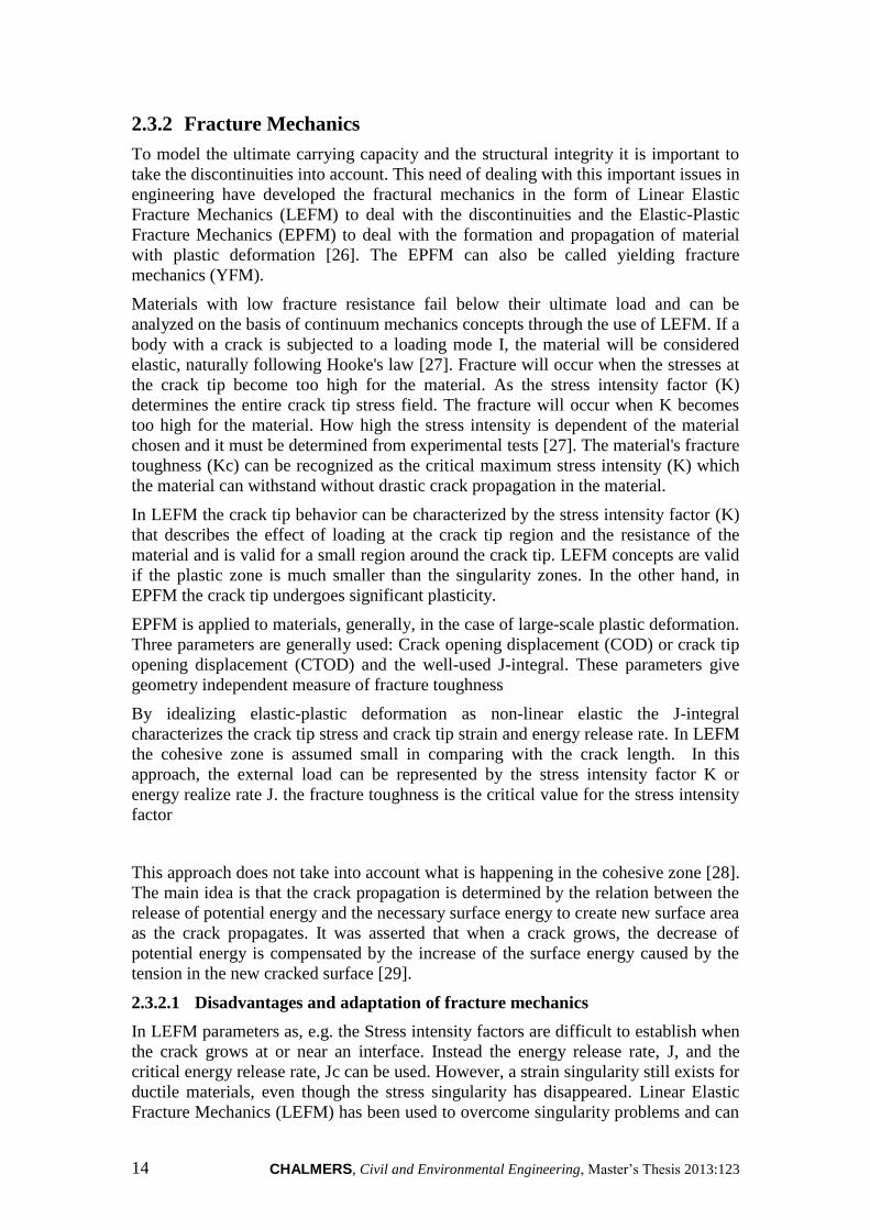
advantages when a relation between moisture concentration and degradation of the
traction-separation law are desired. The main reasons are presented in Table 3.
Table 3 Pros and cons of different mechanical approaches in adhesive joint analysis
Continuum mechanics
Pros:
simple failure criterion
strain criterion is used to predict correct failure
load for brittle adhesives
Describes de normal stresses along and across
the adherents involved.
Cons:
Singularity problems
Mesh dependent
Not apply do describe ductile material
Over estimate the total joint strength
Fracture mechanics
Pros:
Take into account discontinuities
Analysis of both brittle and ductile material is
possible
Geometry independent
Stress intensity factors or energy release rates
describe the singularity zone
Cons:
Need experimental test
Does not take into account the cohesive zone
Predefined crack path gives doubtful results
some times.
Damage mechanics
Pros:
Simulate of damage initiation and propagation
Interfacial failure and cohesive failure are
possible to predict
Various method/approaches exist for both the
traction-separation law and the moisture
dependency.
Proved to give good predictions of the
deformation and failure load
Can be mixed with XFEM
Cons:
The traction-separation laws are obtained true an
empirical process.
The form of the traction-separation law needs to
be modified to experimental results.
The re-adjusting of the parameter is not a
satisfactory way of modeling
Does not explain the physical failure mechanism

CHALMERS Civil and Environmental Engineering, Master’s Thesis 2013:123 19
3 Cohesive zone modeling
Because the moisture concentration affects the adhesive bulk properties, moisture
dependent traction-separation properties are needed for predicting the durability of
adhesive joints. In the work of Katnam [52] the respective experimental test was
carried out to find the traction-separation law for the adhesive in question. Focus was
on the adhesive because the failure mode was cohesive under both wet and dry
situations. Nevertheless, same methodology can be used even if the failure mode is
interfacial failure. In this case the critical energies and traction relates to the degraded
interface strength rather than the bulk material. The diffusion of water along the
interface is often assumed to be faster than in the adhesive material, the interface is
more prone in many cases to moisture consequences than the adhesive [52].
The CZM is ably to describe the interfacial debonding of adhesive joints with a
nonlinear traction-separation relation that simulates the crack opening and growth. A
damage parameter D is used to describe the state of the interface [45].
In the paper [28] Rui Huang discuss the issues of using the CZM for prediction of
interfacial debonding of adhesive joint. There is a conscious that the interfacial failure
mode has been well established theoretically and has been successfully used and
presented in various papers. Nevertheless, the implementation of cohesive elements in
ABAQUS has been discussed. The standard form of the implementation of the
traction-separation laws in ABAQUS differs from many other traction-separation
forms presented in other literate. ABAQUS has the flexibility to use customized
implementation through user subroutines, but this way of modeling is not as straight
forward, as using standard option in the program. However, in the paper of Rui
Huang presents nonlinear traction-separation parameters that are capable of describing
both the initiation process and growth of the adhesive interfacial failure [28]. This
approach can be used to simulate nonlinear material properties as, e.g. nonlinear
viscoelastic and elastic-plastic.
However, to use CZM it’s always needed to first have accurate characterization of the
specific material traction-separation law used, and this is made true experimental
tests. There exist various methodologies how to get the information of the traction-
separation laws for a specific adhesive and different researchers have used different
approaches and methods. In this paper we are going to use the same methodology as
in the work of Liljedahl and Crocombe [7, 14-16, 20, 37, 38, 52, 53] where they first
use some test to find the traction-separation law for mode I and mode II and then
calibrate the exponential value alpha for the mixed mode case, using ABAQUS.
These traction-separation parameters are then used to predict the response of an
overlap tests, a different one from the one used to find the traction-separation
parameters. In this work the Double cantilever beam test (DCB-test) is used to find
the mode I traction separation law, the End notch flexure test (ENF-test) to find the
Mode II traction-separation laws and finally the Mixed Mode cantilever beam test
(MCB-test) to find a realistic value of the exponential parameters “alpha”. In this
work the test results from the work of Saeed Salimi [29] are used and explained in
chapter 5.

CHALMERS, Civil and Environmental Engineering, Master’s Thesis 2013:123 20
3.1 The traction-separation law:
The traction-separation law describes the relationship between the forces of attraction
and the correspondent displacement between the atoms in a material or the adhesively
bonded faces of two equal/different materials [16, 29, 31, 33, 34, 53-56]. The
background to all the equations presented in this chapter is well described in the work
of Saeed Salimi and others [29, 32, 33, 54, 57]. The traction-separation law gives the
information of when the material is in the linear-elastic region, damage initiation and
material failure is reached. The material is in the linear-elastic region until the stresses
or traction reaches Tn,max. When the stresses are equal to Tn,max damage initiation have
started. Total failure is presented when deformation is equal to wc (normal
deformation) or vc (shear deformation).
The model that describes both normal and shear effects acting together is called mix-
mode. The damage initiation for mix-mode used in this work is called quadratic
nominal stress (QUADS) in ABAQUS and is presented as Eq. 2.
The following statements are conceptually presented in Figure 8.
(⟨ ⟩
)
(
)
(
)
Eq. 2
a) b)
Figure 8 a) Traction-separation law for mode I and mode II. b) Traction-separation law
for mix-mode

CHALMERS Civil and Environmental Engineering, Master’s Thesis 2013:123 21
3.1 Traction-separation for pure Mode I
Figure 9 Bilinear traction-separation law for pure mode I.
Damage inititation, propagation and failure (Eq. 3)
{
Eq. 3
Damage parameter D (Eq. 4)
Eq. 4
The tensile stress is related to the opening displacement linearly (Eq. 5)
Eq. 5
Eq. 6 is the same as Eq. 5 expresses in terms of the initial (w0) and critical (wc)
displacement
Eq. 6
From Eq. 5 and Eq. 6 it is noticed that the stress decreases linearly with the
displacement and obviously when which indicates that
the traction-separation element is fully fractured. During unloading, and D
remain constant. Therefore, the stress decreases linearly as the opening displacement
decreases, with the slop .

CHALMERS, Civil and Environmental Engineering, Master’s Thesis 2013:123 22
The energy release rate is the area under the traction-separation curve (Eq. 7) for pure
mode I.
Eq. 7
The experimental test that is well used to obtain the traction-separation for pure mode
I is the DCB-test. The methodology used between the mechanical theory and the
experimental test are well described in the work of Saeed Salimi [29] and is here
summarised in chapter 5. The principal equations are presented below for
completeness.
The form of energy release rate, also called the J-integral that is used for the pure
model I for a thick adhesive layer is presented as (Eq. 8)
Eq. 8
A second expression is used to obtain the traction normal stresses for mode I. This
expression is obtained by differentiating J with respect to the peel deformation w and
is presented as (Eq. 9)
{
}
Eq. 9
These two equations (Eq. 8and Eq. 9) are used to obtain the traction-separation law
for pure mode I. The equation Eq. 8 is used to get the value of the energy release rate
and the stress equations is used to finally get the values of the damage initiation for
pure mode I. However, it is first necessary to perform the DCB-test and get the values
of the force (F), the rotation angle ( ) and the normal deformation (w).

CHALMERS Civil and Environmental Engineering, Master’s Thesis 2013:123 23
3.2 Traction-separation for pure Mode II
The traction-separation behaviour for mode II is basically the same as for the mode I.
Figure 10 Bilinear traction-separation law for pure mode II.
Damage inititation, propagation and failure (Eq. 10)
{
Eq. 10
The damage parameter (Eq. 11)
Eq. 11
The shear stress is related to the displacement linearly (Eq. 12)
Eq. 12
The critical energy release rate is the area under the traction-separation curve in
Figure 12 and the expression (Eq. 13)
Eq. 13
To obtain the traction-separation law for pure mode II, as for mode I, it is first
necessary to perform experimental tests. The test that is used for this purpose is the
ENF-test. Just the results are is used in this work, more information can be found in
the work of Saeed Salimi [29].

CHALMERS, Civil and Environmental Engineering, Master’s Thesis 2013:123 24
In comparison to the expression of the J-integral for mode I, the analytical
formulation of the en integral is a bit more complicated. However the most of the
values in the expression are constant that are dimensions of the ENF-test.
The J-integral that is used for the pure model I for a thick adhesive layer is presented
as (Eq. 14)
Eq. 14
The first part of the (Eq. 14) is the (Eq. 15)
[(
)
(
) ]
Eq. 15
The second part of the (Eq. 14) is the Eq. 16
The following expression is used to obtain the traction shear stresses for mode II. This
expression is obtained by differentiating J with respect to the peel deformation v and
is presented as (Eq. 17)
[
(
)
]
( )
(
)
Eq. 17
[
(
) ]
Eq. 16

CHALMERS Civil and Environmental Engineering, Master’s Thesis 2013:123 25
3.3 Mixed Mode (Mode I and Mode II)
There exist a relation between the shear and normal deformation and this can be
called, the direction variable. The direction variable can be seen as the respective
portions of the total deformation of the shear (v) and normal deformation (w) in
Figure 11. The total deformation is: √ And the direction variable for
shear (Eq. 26) and tensile (Eq. 27) deformation can be expressed like:
√
Eq. 18
√
Eq. 19
Figure 11 Direction variable concept
Therefore the shear and tensile deformation can be expressed as in (Eq. 20) and (Eq.
21)
√ Eq. 20
√ Eq. 21
The damage initiation under mixed mode loading can occur before the shear and
tensile components reach there critical value ( , therefore the damage
initiation is expressed as in (Eq. 22and is called the quadratic nominal stress criterion
(⟨ ⟩
)
(
)
Eq. 22
Or the power law used in ABAQUS, where the exponential value alpha is a variable
that can be identify by experimental test ore re-adjusted to best fit experimental data.
(⟨ ⟩
)
(
)
Eq. 23

CHALMERS, Civil and Environmental Engineering, Master’s Thesis 2013:123 26
And the damage initiation for the mixed mode (Eq. 24)
√
Eq. 24
The damage parameter for mixed-mode is determined by (Eq. 25)
Eq. 25
Figure 12 Bilinear traction-separation law for mix-mode
Where δc is the critical effective displacement, depending on the mixed mode of
Mode I and Mode II of the traction-separation law and δmax is the maximum Mixed
Mode separation displacement during the hole loading history.
Under Mixed Mode loading, both the strength and toughness depend on the direction
of the variable. The Mixed Mode strength depends on the normal and shear strenght
and consequently the mixed mode toughness depends on the Mode I and Mode II
toughness. Toghether at least five parameters are needed to describe the fracture.
Stiffness ( ), (Eq. 26)
Normal and shear strength . (Eq. 12) and (Eq. 9)
Toughness given the mixed mode energy release rate (Eq. 27)
[
] Eq. 26

CHALMERS Civil and Environmental Engineering, Master’s Thesis 2013:123 27
Eq. 27
One form of expressing the is shown in (Eq. 28)
{
(
)
(
)
}
Eq. 28
where and Critical energy release rate for pure mode I and mode II
Expressing the critical energy release rate with the direction variable (Eq. 29)
{(
)
(
)
}
Eq. 29
And the critical separation displacement with respect to the direction variable in
mixed mode (Eq. 30)
In CZM in ABAQUS the direction variable is defined locally at each point or for each
interface element. Therefore the mode mix may change along the interface and during
the loading process. Too model the critical energy release rate with respect to the
direction variable Ψ it is necessary to use the power law fracture criterion:
{
}
{
}
Eq. 31
The necessary experimental tests to be performed for the traction-separation
parameters in mixed-mode are in principal a test that describes the behavior of both
modes together.
The test results used in this work are from a MCB-test performed by Saeed Salimi
[29]. The equations that are needed together with the MCB-tests are:
Vertical force at the crack tip, where S is the applied force with angle beta (Eq. 32).
Eq. 32
{(
)
(
)
}
Eq. 30

CHALMERS, Civil and Environmental Engineering, Master’s Thesis 2013:123 28
Normal force at the crack tip (Eq. 33)
Eq. 33
Moment at the crack tip (Eq. 34).
Eq. 34
The energy release rate for the MCB-test is(Eq. 35).
Eq. 35
Inserting the sectional forces and moment in to the expression of JMCB gives (Eq. 36)
[
(
)
]
Eq. 36

CHALMERS Civil and Environmental Engineering, Master’s Thesis 2013:123 29
4 Modeling of moisture distributions in adhesive
joints
In this study, one of the main objectives is to analyse the effects of moisture in
adhesive joints, and be able to quantify the degradation induced by the adhesive, and
the corrosion of the steel in contact with the adhesive. Therefore, a good model to find
the moisture concentration in the adhesive joint with respect to time in a specific
environment is needed. As the moisture diffusion depends on the moisture
concentration, and the moisture concentration varies in each dimension of the
adhesive, we are taking in consideration two kind of moisture diffusion: adhesive
layer diffusion and interface diffusion.
For this study, 3 different kinds of environments have been used: one with 23ºC and
immersed one with 43 º C and immersed and one with 43ºC and with 95% Relative
humidity, trying to simulate critical spots in the bridge where water could accumulate.
To increase the effect of corrosion, all the environmental chambers have a 5% of
NaCl content. This is justified because in countries with cold climates, salt is used to
prevent the freezing of the road. Eventually, this salt falls off to the steel structure of
the bridge, and it expected that 5% of salt content is a good approximation of this
effect.
4.1 Theory background
4.1.1 Fickan model
Moisture diffusion is analogous to heat transfer, since both are caused by random
molecular motions. Fick adopted Fourier’s mathematical expression for heat
conduction to quantify the diffusion [58]. Fick’s first law is:
Eq. 37
Where Fx is the diffusion flux in the x direction, D is the diffusion coefficient, and
is the concentration gradient. The expression is negative because diffusion occurs in
the opposite direction of increasing concentration. Also, this equation is only valid for
isotropic medium.
Fick’s second law describes the nonsteady state of diffusion and can be derived from
Fick’s first law. Crank [59] has shown that for a constant diffusion coefficient, it is
obtained:
(
)
Eq. 38

CHALMERS, Civil and Environmental Engineering, Master’s Thesis 2013:123 30
where C is the concentration of the diffusing substance and D is the diffusion
coefficient. The previous expression can be simplified for a one-dimensional diffusion
to:
(
)
Eq. 39
The solution for this one-dimensional equation that calculates the concentration of a
diffusing substance in an isotropic plane sheet of finite thickness depending on time
and space is:
∑
[
]
Eq. 40
where D is the diffusion coefficient, is the half-thickness of the sheet (- <x< ), C is
the concentration of the diffusing substance at position x and time t, and C∞ is the
saturation concentration of the absorbed substance. This equation assumes that the
concentration at the borders is the saturation concentration, the initial concentration of
the diffusing substance is zero, and the diffusion coefficient remains constant. An
analogous expression based on mass diffused, according to Crank [59] is:
∑
[
]
Eq. 41
where D is the diffusion coefficient, h is the total sheet thickness, Mt is the total mass
absorbed by the sample at a time t, and M∞ is the equilibrium mass of the absorbed
substance.

CHALMERS Civil and Environmental Engineering, Master’s Thesis 2013:123 31
4.1.2 Two dimensional equation
The diffusion of moisture in the adhesive can’t be considered as one-dimensional,
because in this case our adhesive layer is free in 2 axes. Therefore, a two dimensional
equation is needed in order to calculate the ingress of moisture by the faces of the
adhesive that are exposed to the environment.
The concentration of moisture, depending on 2 space variables (x,y) and time, being
the adhesive layer a rectangle with thickness in the z axis, can be written as:
∑ ∑
[
(
)
(
)
]
Eq. 42
where x and y are the distances from the centre of the adhesive layer, x0 and y0 are the
total dimensions of the adhesive layer in that direction, is the half-thickness of the
sheet, D is the diffusion coefficient and t is the time.
4.1.3 Different mass uptake equations
4.1.3.1 Non Fickian
It has been observed that polymers present non-Fickian behaviour when the
temperature is below the glass transition temperature (Tg) [58], where the diffusion
process differs from Fickian behaviour after initial uptake. The two mechanisms of
the dual Fickian model are considered to be working in parallel. The one-dimensional
equation for the non-Fickian behaviour [59] that determinates the concentration is:
(
∑
[
]
)
(
∑
[
]
)
Eq. 43
where C1∞ and C2∞ are fractions of saturated concentration C∞, D1 and D2 are the
diffusion coefficients and is the length of the diffusion path.
The mass uptake equation in the non-Fickian model is:
(
∑
[
]
)
(
∑
[
]
)
Eq. 44
where M1∞ and M2∞ are fractions of saturated mass uptake M∞.

CHALMERS, Civil and Environmental Engineering, Master’s Thesis 2013:123 32
4.1.3.2 Relaxation of the adhesive
At high temperatures, and for adhesives immersed in liquids, a phenomenon of
polymer relaxation takes place. This mechanism increases the water uptake of the
adhesive. According to [58] the equation that considers the polymer relaxation is:
{ [ (
)
]}
Eq. 45
This equation considers both the Fickian behaviour and the polymeric relaxation
taking place in the adhesive. The first part considers the Fickian diffusion and when
the curve starts to bend over, and then the relaxation part has the dominance of the
moisture ingress. The final moisture saturation level M∞ is the sum of the absorption
during Fickian process, M∞,F and the maximum absorption due to polymer relaxation,
M∞,R.
4.1.3.3 Delayed dual Fickian model
Sometimes, the experimental data doesn’t fit with any of the previous models
explained before when there is a secondary uptake. To incorporate the secondary
uptake in the analytical model, a dual Fickian model with a Heaviside step function
can be used. This model is called delayed dual Fickian model, where the secondary
uptake is modelled by power law [59]. The expression is:
(
∑
[
]
)
(
∑
[
]
)
( )
Eq. 46
where is the Heaviside step function, t1 is the start time of secondary uptake as
determined experimentally and a,b and c are toe power law constants determined by
curve fitting.

CHALMERS Civil and Environmental Engineering, Master’s Thesis 2013:123 33
4.2 Experimental test and results
4.2.1 Gravimetric test
For this moisture diffusion in the adhesive layer, a gravimetric test has been
performed in order to obtain the diffusion coefficient (D). This test method covers the
determination of the relative rate of absorption of water by plastics when immersed,
and has two chief functions: first, as a guide to the proportion of water absorbed by a
material; and second, as a control test on the uniformity of a product. Ideal diffusion
of liquids into polymers is a function of the square root of immersion time. Time to
saturation is strongly dependent on specimen thickness. The experiment consisted in
immersing an adhesive specimen of 60x60x1 mm in water, according to the ASTM D
570 – 98 standard[36], and then measures of the water uptake are taken.
4.2.2 Gravimetric test results
As this thesis aim is to develop a methodology and not to go into tests and values, it is
going to be assumed a value of D, the one that was obtained in the work of Nguyen
[32], with a value of 2.07·10-7
mm2/s.

CHALMERS, Civil and Environmental Engineering, Master’s Thesis 2013:123 34
4.3 Verification of our model
4.3.1 Finite element method and analytical method
To prove the accuracy of the ABAQUS results, Fickian concentration equation was
modelled in MATLAB (see Appendix A), so a comparison between a numerical
solution and an analytical solution could be done. The 2D diffusion equation was used
in MATLAB, while the Mass Diffusion module was used in ABAQUS. Both methods
need as an input the diffusion coefficient and the maximum concentration, which can
be obtained from a gravimetric test.
Figure 13 Comparison of diffusion profile performed by MATLAB and ABAQUS
As it can be appreciated in the previous graphic, the ABAQUS (FEM) and the
MATBAL (analytical) solutions are the same, therefore the FEM model is validated.
4.3.2 Analogy between heat and moisture
The Finite Element program ABAQUS can´t do a coupled stress-mass diffusion
analysis. In order to perform this analysis, an analogy between heat transfer and mass
diffusion shall be done. According to Fourier’s law of heat conduction:
Eq. 47
where q(W m-2
) is the heat flux, k(W m-1
K-1
) is the conductivity, ∇T(K m-1
) is the
temperature gradient. From this equation, Fick developed his first law of diffusion:
Eq. 48
Mois
ture
co
nce
ntr
ati
on
Distance from edge (mm)
ABAQUS
MATLAB

CHALMERS Civil and Environmental Engineering, Master’s Thesis 2013:123 35
where Fx is the diffusion flux in the direction x, D is the diffusion coefficient and
C/ x is the concentration gradient. To relate these two equations, a transformation is
needed to make the heat conduction to be heat diffusion, to be like the Fick’s law. In
order to do that, the conductivity parameter k has to be converted into a diffusion
parameter, DT. Using Lewis formula:
Eq. 49
where αc is the convective heat transfer coefficient, ρ(kg m-3
) is the density and cp(J
kg-1
K-1
) is the heat capacity. Using this formula, the conductivity k(W m-1
k-1
)
becomes a diffusion coefficient DT(m2 s
-1) as follows:
Eq. 50
In ABAQUS, to model the mass diffusion, the solubility, the concentration and the
diffusion are needed to be introduced. In order to get the same results in the heat
transfer analysis, the conductivity of the adhesive is introduced as the diffusivity, and
both the density and the specific heat are introduced as 1. It is important, though, to
introduce a really low value of the heat capacity in both the CFRP and the steel (for
example 1e-06) in order to avoid the heat to diffuse through this materials.
With this method, both the mass diffusion module and the heat transfer module give
the same results, and as the mass diffusion was validated with the analytical solution,
this means that the heat transfer solution is also correct.

CHALMERS, Civil and Environmental Engineering, Master’s Thesis 2013:123 36

CHALMERS Civil and Environmental Engineering, Master’s Thesis 2013:123 37
5 Experiments
As it was discussed in chapter 3, when the choice is to use CZM to predict an
adhesive joint behavior it is first necessary to perform tests to obtain the traction-
separation laws for the actual adhesive in question. The traction-separation law for
pure mode I, mode II and the exponential value alpha for the power law are obtained
true the test described in the table below Table 4. Mode III is assumed to be equal to
mode II.
Table 4 Test that is used to obtain the traction-separation law for mode I, mode II and
mix-mode.
Do
ub
le Can
tilever B
eam
test
DC
B-test
End
No
tch Fle
xure test
ENF-te
st
Mixed
-mo
de C
antilever B
eam
MC
B-te
st

CHALMERS, Civil and Environmental Engineering, Master’s Thesis 2013:123 38
The test used for mode I is the DCB-test, for mode II the ENF-test and for the
exponential value alpha the MCB-test Table 4. The dimensions used for these
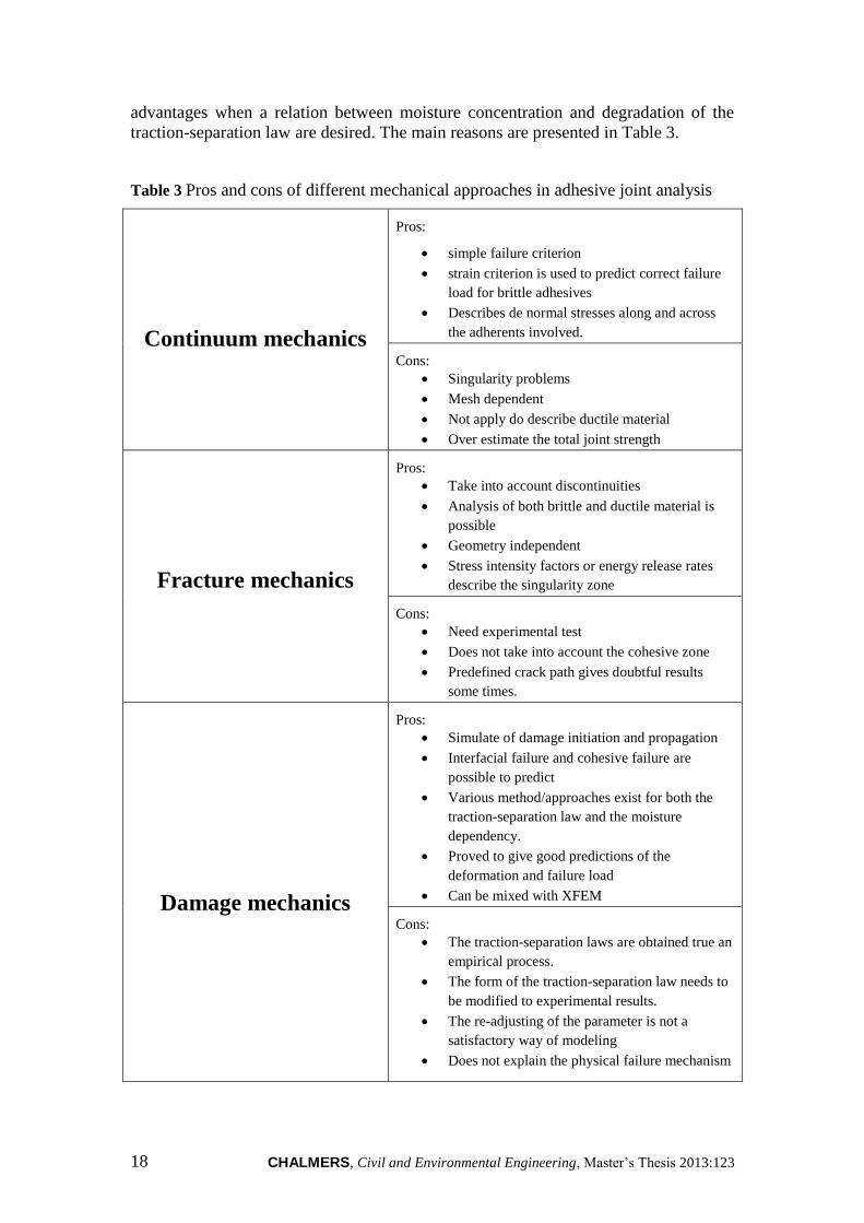
different tests are presented in table Table 5. The TRB and DLS test are made for the
verification of the ABAQUS models and are shown in Table 6 and the corresponding
dimensions are presented in Table 7.
Table 5 Dimensions of test used and performed in this work.
Table 6 RTB and DLS-joint
TRB-joint
DLS-joint, taking 1/4 of the total geometry for simplicity
Type h [mm] a0 [mm] b [mm] l [mm] t [mm] No. of
specimen
DCB 6.6 80 8.3 200 2.4 3
ENF 16.6 350 16.6 1000 2.4 3
MCB 10 25 4 125 2.4 6

CHALMERS Civil and Environmental Engineering, Master’s Thesis 2013:123 39
Table 7 Dimensions for the RTB and DLS-joint
TRB h1 h2 t f g db c L1 L2
Dim. 10 4 2.4 90 10 215 10 280 330
DLS h1 h2 h3 l1 l2 l3 bsteel bCFRP badhesive
Dim. 1.25 1.45 5 205 200 300 60 50 50
The steel used for TRB-joints haves an elastic modulus of 196 GPa.
5.1 DCB-test results
As in the work of Saeed Salimi [29] the results from the DCB-test are used to find the
traction-separation law for pure mode I. The experimentally measured value of F, w
and theta together with the corresponding equations gives the characteristic curves
that are wanted.
Table 8 Process from the experimental outcome to the traction-separation law
The differentiation of JDBC to obtain σ(w) causes a substantial scatter, consequently,
the JDBC = J(w) data is fitted with a polynomial of order k ore a Prony-series with k
terms.
∑
∑ (
)
Polynomial-series Prony-series
Experimental output:
Force and deflection
(F and w)
J-w curve from the use of
the equation JDCB and the
experimental output.
{
}
Differentiation of JDCB to
obtain the curve: stress vs.
deformation

CHALMERS, Civil and Environmental Engineering, Master’s Thesis 2013:123 40
Table 9 Traction-separation law from the test and analytical expressions.
Experiment
No. [
]
1 930 24 52 2.6
2 1010 20 69 2.1
3 1020 23 69 4.2
Mean value 987 22 63 3
5.2 ENF-test results
As for the DCB-test, the same methodology is used for the ENF-test. The
experimentally measured value of F and v together with the corresponding equations
gives the characteristic curves that are wanted.
Table 10 Process from the experimental outcome to the traction-separation law
Experimental output:
Force and deflection (F
and w.
J-v curve from the use of
the equation JENF and the
experimental results.
Differentiation of JENF to
obtain the curve: shear vs.
deformation
The differentiation of JENF to obtain τ(v) causes a substantial scatter, consequently, the
JENF = J(v) data is fitted with a polynomial of order k ore a Prony-series with k terms
∑
∑ (
)
Polynomial-series Prony-series

CHALMERS Civil and Environmental Engineering, Master’s Thesis 2013:123 41
Table 11 Traction-separation law from the test and analytical expressions.
5.3 MCB-test results
The outcomes from the MCB-test are recorded with the ARAMIS 4M system. The
displacement of four point at the crack tip are measured in order to determinate the
shear and peel deformation of the adhesive layer and the rotation of the adherent. The
displacement is measured in both x and y directions and the rotation are evaluated
with equations showed in Figure 14.
a) b)
Figure 14 a) Positions of the points used to record the displacement at the crack tip.
b) Equations used to evaluate the rotation
Figure 15 Rotational angel of the over (blue) and under (red) adherents vs. the
displacement
Experiment
No. [
]
1 2.99 28.4 264 1.1
2 3.57 26.6 211 1.1
3 4.35 28.2 255 1.2
Mean value 3.64 27 243 1

CHALMERS, Civil and Environmental Engineering, Master’s Thesis 2013:123 42
In the work of Saeed Salimi [29] it is shown that when comparing the MCB
simulation results in ABAQUS with the experimental results presented above the best
value of the exponential parameter alpha in Eq. 2 is 0.8. When defining the material
properties in edit material in ABAQUS, damage initiation (QUADS DAMAGE) and
in the damage propagation option (DAMAGE EVOLUTION) the power law is chosen
as the mix mode behavior and the exponential value as 0.8.
Figure 16 Exponential value alpha in ABAQUS

CHALMERS Civil and Environmental Engineering, Master’s Thesis 2013:123 43
In the MCB-test the shear and peel deformation is recorded with the help points
shown in Figure 14 and Eq. 51 and Eq. 52. The shear and peel deformation is
conceptually presented in Figure 17 and the results from the test are compare with the
simulation in ABAQUS with different values of alpha. This iteration process gives an
indication of witch value of alpha to use for the prediction of failure load for the test
specimens presented in chapter 5.5 and 5.6.
Figure 18 shears and peel deformation, experimental versus simulations with
different alpha values.
( ) Eq. 51
( ) Eq. 52
Figure 17 shear and peel deformation

CHALMERS, Civil and Environmental Engineering, Master’s Thesis 2013:123 44
Another comparison that is maid between the simulation in ABAQUS and test results
is the force versus displacement. The conceptual relation is shown in Figure 19.
Figure 19 Force vs. displacement at crack tip. Where S is the applied external force
on the joint specimen.
Figure 20 Force vs. displacement, experimental versus simulations with different
alpha values.
Finally a comparison is maid between the energy release rate and displacement is
done and the conceptual relation is shown in Figure 21. Inserting the sectional forces
and moment in to (Eq. 36) gives the experimental results and is presented in Figure
22, this is also compared with different values of alpha.

CHALMERS Civil and Environmental Engineering, Master’s Thesis 2013:123 45
Figure 21 Energy release rate vs. displacement at the crack tip.
Figure 22 Energy release rate vs. displacement, experimental versus simulations with
different alpha values.

CHALMERS, Civil and Environmental Engineering, Master’s Thesis 2013:123 46
5.4 TRB-test
The TRB-test results are used to compare the failure load obtained in the simulation
of the TRB-joint analysis performed in ABAQUS. In this Chapter the TRB-joint test
performance is described and the results are summarized. Three test specimens are
used and the results are shown in Figure 25 and Table 12 TRB test results.
For the set of specimens, due to a technical problem with the internal LVDT, an
external LVDT was used to measure the displacement of the loading point Δ, as
shown in figure below. The displacement rate of the loading point has been set at
2mm /min for all experiments.
Figure 23 TRB specimen being tested
Figure 24 TRB specimen being tested

CHALMERS Civil and Environmental Engineering, Master’s Thesis 2013:123 47
Figure 25 Experimental results for TRB
Table 12 TRB test results
Test specimen Failure load (N) Failure deformation (mm)
TRB1 4850 4.1
TRB2 4500 4.0
TRB3 4500 4.2
Fo
rce
Deformation
TRB3
TRB2
TRB1

CHALMERS, Civil and Environmental Engineering, Master’s Thesis 2013:123 48
5.5 DLS test
The DLS-test is performed to verify the methodology presented in this work. In this
Chapter the DLS-joint manufacturing process is presented and the results are
summarized at the end. The comparison of test results and the simulation in ABAQUS
are well described in Chapter 6.
Two test specimens where tested. The test specimens are named CSt1 and CSt2.
To perform the DLS tests, wood molds were first created in order to maintain the
geometry of the samples. The adhesive was poured inside this mold and a constant
thickness of 1.5mm was achieved applying pressure in the upper part of the mold, as
the excess of adhesive was being removed from the sample.
Figure 26 DLS-joint
Figure 27 DLS mould configuration

CHALMERS Civil and Environmental Engineering, Master’s Thesis 2013:123 49
After making the specimens in the mold, they were left inside the mold for 2 days.
After that, they were taken outside de mold and left for 1 week for curing. Next image
shows a finished DLS sample.
Figure 29 DLS specimen curing
Figure 28 DLS molds with the CFRP in place

CHALMERS, Civil and Environmental Engineering, Master’s Thesis 2013:123 50
After curing, the samples were pulled, and a load-displacement curve was obtained.
The speed of pulling was 0.1 mm/min.
Figure 30 DLS specimen being pulled
Figure 32 Cohesive failure in the specimens

CHALMERS Civil and Environmental Engineering, Master’s Thesis 2013:123 51
Figure 31 Specimens after the test
Table 13 Results of failure loads and failure modes for the tested DLS-joint samples.
Test specimen Failure
mode
Failure load
(N)
Failure deformation (mm)
Exp 1 mix-mode 140000 1.5
Exp 2 mix-mode 135000 1.4
Exp 3 mix-mode 125000 1.1
CHALMERS, Civil and Environmental Engineering, Master’s Thesis 2013:123 52
Figure 32 DLS-test results

CHALMERS Civil and Environmental Engineering, Master’s Thesis 2013:123 53
6 Finite element modeling and analysis
It is now possible to use the traction-separation law obtained from the experimental
test. The traction-separation laws for mode I and II from DCB and ENF-tests, and the
estimated value of the exponential value alpha for the power law from the MCB-test.
This is now all used and applied the finite element analysis program. The aim is to
predict the failure load of the dry DLS-test and TRB-test and compare them with
experimental data and in that way verifying the CZM approach.
The finite element analysis program ABAQUS version 6.11-1 was used for numerical
modeling.
6.1 Material properties
Typical steel mechanical properties (E=210 GPa and ν=0.29) were used for the steel
plates. To model the CFRP, the elastic parameters E=135 GPa and ν=0.3 were
defined. When the adhesive is not completely considered as a cohesive element, its
properties are E=7 Gpa and ν=0.3.
6.2 CZM parameters
To simulate the specimens in ABAQUS (both the TRB and the DLS) using the
Cohesive Zone Modeling approach, ABAQUS uses cohesive elements. Using
cohesive elements imply that the choice of material properties and section type is
consistent with the type of cohesive element. The material properties of the adhesive-
cohesive layer are chosen as traction, and have defined a damage initiation (QUADS
DAMAGE in ABAQUS) and in the damage propagation option (DAMAGE
EVOLUTION in ABAQUS) the power law is chosen as the mix mode behavior and
the exponential. The section type is also set as cohesive. In this analysis the type of
stress-strain relation is the uncoupled and is as follow:
{
} [
] {
}
Eq. 53
For the uncoupled behavior each traction component depends only on its conjugate
nominal strain. The Eq. 53 has the quantities of the nominal tractions in the normal
and in the two local shear directions at the left side of the equation. The matrix is the
elasticity in terms of traction and separations for cohesive elements and the
corresponding nominal strains are in the right side of the matrix.
To simulate the tests ABAQUS need the following input:
Elastic properties of the adhesive layer are set to traction Table 14. The Damage
initiation definition is presented in Table 15 and the damage propagation in Table 16.
The damage Stabilization (VISCOSITY COEFFICIENT) is set to 0.0001.

CHALMERS, Civil and Environmental Engineering, Master’s Thesis 2013:123 54
Table 14 Elastic properties
E or Knn G1 or Kss G2 or Ktt
Table 15 Damage initiation (QUADS DAMAGE)
Nominal stress normal-
only mode
Nominal stress first
direction
Nominal stress second
direction
(Damage initiation for
pure mode I)
(Damage initiation for
pure mode II)
(Damage initiation for
pure mode II)
Table 16 Damage propagation (DAMAGE EVOLUTION)
Normal mode Fracture
energy
Shear mode Fracture
energy first direction
Shear mode Fracture
energy Second direction
[
] [
] [
]
6.3 TRB-joint simulation
6.3.1 Description of the models
Figure 33 different models that are used for the TRB simulation
Model Adhesive
layers Adhesvie
joint
TRB only one
layer
Adhesvie-Cohesive
Tolerance
Cohesive
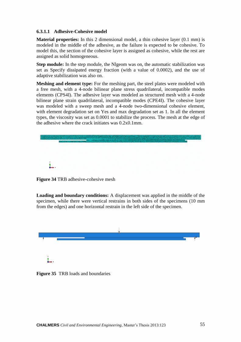
CHALMERS Civil and Environmental Engineering, Master’s Thesis 2013:123 55
6.3.1.1 Adhesive-Cohesive model
Material properties: In this 2 dimensional model, a thin cohesive layer (0.1 mm) is
modeled in the middle of the adhesive, as the failure is expected to be cohesive. To
model this, the section of the cohesive layer is assigned as cohesive, while the rest are
assigned as solid homogeneous.
Step module: In the step module, the Nlgeom was on, the automatic stabilization was
set as Specify dissipated energy fraction (with a value of 0.0002), and the use of
adaptive stabilization was also on.
Meshing and element type: For the meshing part, the steel plates were modeled with
a free mesh, with a 4-node bilinear plane stress quadrilateral, incompatible modes
elements (CPS4I). The adhesive layer was modeled as structured mesh with a 4-node
bilinear plane strain quadrilateral, incompatible modes (CPE4I). The cohesive layer
was modeled with a sweep mesh and a 4-node two-dimensional cohesive element,
with element degradation set on Yes and max degradation set as 1. In all the element
types, the viscosity was set as 0.0001 to stabilize the process. The mesh at the edge of
the adhesive where the crack initiates was 0.2x0.1mm.
Figure 34 TRB adhesive-cohesive mesh
Loading and boundary conditions: A displacement was applied in the middle of the
specimen, while there were vertical restrains in both sides of the specimens (10 mm
from the edges) and one horizontal restrain in the left side of the specimen.
Figure 35 TRB loads and boundaries

CHALMERS, Civil and Environmental Engineering, Master’s Thesis 2013:123 56
6.3.1.2 Tolerance model
Material properties: The steel was modeled as solid homogeneous, while the
adhesive layer was modeled completely as cohesive elements. In this model, to avoid
assigning viscosity to the material, a tolerance of 0.2 is chosen.
Step module: In the step module, the Nlgeom was on, the automatic stabilization was
set as Specify dissipated energy fraction (with a value of 0.0002) and the use of
adaptive stabilization was also on.
Meshing and element type: For the meshing part, the steel plates were modeled with
a structured mesh, with a 4-node bilinear plane stress quadrilateral, reduced
integration, hourglass control elements (CPS4R). The cohesive layer was modeled
with a sweep mesh and a 4-node two-dimensional cohesive element, with all the
options set as default. There was only 1 element in the thickness of the adhesive layer.
The overall mesh was 1mm.
Figure 36 TRB tolerance mesh
Loading and boundary conditions: A displacement was applied in the middle of the
specimen, while there were vertical restrains in both sides of the specimens (10 mm
from the edges) and one horizontal restrain in the left side of the specimen.
6.3.1.3 Cohesive model
Material properties: The steel was modeled as solid homogeneous, while the
adhesive layer was modeled completely as cohesive elements.
Step module: In the step module, the Nlgeom was on, the automatic stabilization was
set as Specify dissipated energy fraction (with a value of 0.0002) and the use of
adaptive stabilization was also on.
Meshing and element type: For the meshing part, the steel plates were modeled with
a structured mesh, with a 4-node bilinear plane stress quadrilateral, incompatible
modes elements (CPS4I). The cohesive layer was modeled with a sweep mesh and a
4-node two-dimensional cohesive element (COH2D4), with element degradation set
on Yes and max degradation set as 1. In all the element types, the viscosity was set as
0.0001 to stabilize the process. There was only 1 element in the thickness of the
adhesive layer. The overall mesh was 1mm.

CHALMERS Civil and Environmental Engineering, Master’s Thesis 2013:123 57
Figure 37 TRB cohesive mesh
Loading and boundary conditions: A displacement was applied in the middle of the
specimen, while there were vertical restrains in both sides of the specimens (10 mm
from the edges) and one horizontal restrain in the left side of the specimen.
Figure 38 Test and simulation results for TRB
P (
N)
Δ (mm)

CHALMERS, Civil and Environmental Engineering, Master’s Thesis 2013:123 58
6.4 DLS-joint simulation
To model the DLS samples, a 2D model was firstly used, and finally a 3D model was
also performed to compare the results. For the 2D models, 3 different hypotheses were
tested: all the adhesive layers may fail, just one side of the DLS may fail or 2 adhesive
layers in diagonal may fail.
6.4.1 Description of the 2D models
Figure 39 Different models that are used for the DLS simulation
Model Adhesive
layers Adhesvie
joint
DLS
All 4 layers
2 layers in one side
Adhesive-Cohesive
Tolerance
Cohesive
Kinematic
2 layers, one on each side in
diagonal

CHALMERS Civil and Environmental Engineering, Master’s Thesis 2013:123 59
6.4.1.1 Four cracks model
6.4.1.1.1 Cohesive model
Figure 40 DLS 4 cracks cohesive
Material properties: The steel and the CFRP were modeled as solid homogeneous,
while all the adhesive layers were modeled completely as cohesive elements.
Step module: In the step module, the Nlgeom was on, the automatic stabilization was
set as Specify dissipated energy fraction (with a value of 0.0002) and the use of
adaptive stabilization was also on.
Meshing and element type: For the meshing part, the steel plates were modeled with
a structured mesh, with a 4-node bilinear plane stress quadrilateral, incompatible
modes elements (CPS4I). The cohesive layer was modeled with a sweep mesh and a
4-node two-dimensional cohesive element (COH2D4), with element degradation set
on Yes and max degradation set as 1. In all the element types, the viscosity was set as
0.0001 to stabilize the process. There was only 1 element in the thickness of the
adhesive layer. The overall mesh was 0.5 mm.
Figure 41DLS cohesive mesh
Loading and boundary conditions: The DLS sample was fixed in one side and was
being pulled from the other, so the boundary conditions assigned in this model were
fixing all the displacements in one edge and assigning a displacement to the other
edge. The reaction forces were obtained by summing the value of the RF in all the
nodes that were fixed.
Figure 42 Standard boundary conditions

CHALMERS, Civil and Environmental Engineering, Master’s Thesis 2013:123 60
6.4.1.1.2 Adhesive-Cohesive model
Figure 43 DLS 4 cracks adhesive-cohesive
Material properties: The steel and the CFRP were modeled as solid homogeneous,
while the adhesive layers were modeled as 2 layers of solid homogeneous material
with a thin layer of cohesive elements in the middle.
Step module: In the step module, the Nlgeom was on, the automatic stabilization was
set as Specify dissipated energy fraction (with a value of 0.0002) and the use of
adaptive stabilization was also on.
Meshing and element type: For the meshing part, the steel plates were modeled with
a structured mesh, with a 4-node bilinear plane stress quadrilateral, incompatible
modes elements (CPS4I). The adhesive layer was modeled as structured mesh with a
4-node bilinear plane strain quadrilateral, incompatible modes (CPE4I). The cohesive
layer was modeled with a sweep mesh and a 4-node two-dimensional cohesive
element (COH2D4), with element degradation set on Yes and max degradation set as
1. In all the element types, the viscosity was set as 0.0001 to stabilize the process. The
mesh size in the important points was 0.2x0.2 mm, and it grew till 1.5 mm at the
edges of the steel plates.
Figure 44 DLS 4 cracks adhesive-cohesive mesh centre
Figure 45 DLS 4 cracks adhesive-cohesive side

CHALMERS Civil and Environmental Engineering, Master’s Thesis 2013:123 61
Loading and boundary conditions: The DLS sample was fixed in one side and was
being pulled from the other, so the boundary conditions assigned in this model were
fixing all the displacements in one edge and assigning a displacement to the other
edge.
6.4.1.1.3 Tolerance model
Figure 46 DLS 4 cracks tolerance
Material properties: The steel and the CFRP were modeled as solid homogeneous,
while all the adhesive layers were modeled completely as cohesive elements. In
material properties, the cohesive elements have a tolerance of 0.2 instead of the
default 0.05.
Step module: In the step module, the Nlgeom was on, the automatic stabilization was
set as Specify dissipated energy fraction (with a value of 0.0002) and the use of
adaptive stabilization was also on.
Meshing and element type: For the meshing part, the steel plates were modeled with
a structured mesh, with a 4-node bilinear plane stress quadrilateral, incompatible
modes elements (CPS4I). The cohesive layer was modeled with a sweep mesh and a
4-node two-dimensional cohesive element (COH2D4), with element degradation set
on Yes and max degradation set as 1. Instead of entering a viscosity as an input, the
tolerance is the one that stabilizes the process. There was only 1 element in the
thickness of the adhesive layer. The overall mesh was 0.5 mm.
Figure 47 DLS 4 cracks tolerance mesh
Loading and boundary conditions: The DLS sample was fixed in one side and was
being pulled from the other, so the boundary conditions assigned in this model were
fixing all the displacements in one edge and assigning a displacement to the other
edge. The reaction forces were obtained by summing the value of the RF in all the
nodes that were fixed.

CHALMERS, Civil and Environmental Engineering, Master’s Thesis 2013:123 62
6.4.1.1.4 Kinematic model
Figure 48 DLS 4 cracks kinematic
Material properties: The steel and the CFRP were modeled as solid homogeneous,
while the adhesive layers were modeled as 2 layers of solid homogeneous material
with a thin layer of cohesive elements in the middle.
Step module: In the step module, the Nlgeom was on, the automatic stabilization was
set as Specify dissipated energy fraction (with a value of 0.0002) and the use of
adaptive stabilization was also on.
Meshing and element type: For the meshing part, the steel plates were modeled with
a structured mesh, with a 4-node bilinear plane stress quadrilateral, incompatible
modes elements (CPS4I). The adhesive layer was modeled as structured mesh with a
4-node bilinear plane strain quadrilateral, incompatible modes (CPE4I). The cohesive
layer was modeled with a sweep mesh and a 4-node two-dimensional cohesive
element (COH2D4), with element degradation set on Yes and max degradation set as
1. In all the element types, the viscosity was set as 0.0001 to stabilize the process. The
mesh size in the important points was 0.2x0.2 mm, and it grew till 1.5 mm at the
edges of the steel plates.
Figure 49DLS 4 cracks kinematic mesh centre

CHALMERS Civil and Environmental Engineering, Master’s Thesis 2013:123 63
Figure 50 DLS 4 cracks kinematic mesh side
Loading and boundary conditions: The DLS sample was fixed in one side and was
being pulled from the other, so the boundary conditions assigned in this model were
fixing all the displacements in one edge and assigning a displacement to the other
edge. In the displacement side, instead of selecting the whole surface and get the
values of RF for each node, in this model a constraint was included, selecting the
bottom point of the surface as control point and assigning a kinematic coupling to the
surface, so the RF was monitored my only checking this node.
Figure 51 Kinematic model boundaries
6.4.1.1.5 Results
Figure 52 Test and simulation results for the 4 cracks models

CHALMERS, Civil and Environmental Engineering, Master’s Thesis 2013:123 64
6.4.1.2 Two cracks diagonal model
6.4.1.2.1 Cohesive model
Figure 53 DLS 2 cracks diagonal cohesive
Material properties: The steel and the CFRP were modeled as solid homogeneous,
while 2 adhesive layers where considered completely as cohesive elements and the
other ones as adhesive with solid homogeneous properties.
Step module: In the step module, the Nlgeom was on, the automatic stabilization was
set as Specify dissipated energy fraction (with a value of 0.0002) and the use of
adaptive stabilization was also on.
Meshing and element type: For the meshing part, the steel plates were modeled with
a structured mesh, with a 4-node bilinear plane stress quadrilateral, incompatible
modes elements (CPS4I). The cohesive layer was modeled with a sweep mesh and a
4-node two-dimensional cohesive element (COH2D4), with element degradation set
on Yes and max degradation set as 1. In all the element types, the viscosity was set as
0.0001 to stabilize the process. There was only 1 element in the thickness of the
adhesive layer. The overall mesh was 0.5 mm.
Figure 54 DLS 2 cracks diagonal cohesive mesh
Loading and boundary conditions: The DLS sample was fixed in one side and was
being pulled from the other, so the boundary conditions assigned in this model were
fixing all the displacements in one edge and assigning a displacement to the other
edge. The reaction forces were obtained by summing the value of the RF in all the
nodes that were fixed.

CHALMERS Civil and Environmental Engineering, Master’s Thesis 2013:123 65
6.4.1.2.2 Adhesive-Cohesive model
Figure 55 DLS 2 cracks diagonal adhesive-cohesive
Material properties: The steel and the CFRP were modeled as solid homogeneous, 2
of the adhesive layers were modeled as 2 layers of adhesive with a cohesive element
in the middle, while the other 2 were completely modeled as adhesive layers.
Step module: In the step module, the Nlgeom was on, the automatic stabilization was
set as Specify dissipated energy fraction (with a value of 0.0002) and the use of
adaptive stabilization was also on.
Meshing and element type: For the meshing part, the steel plates were modeled with
a structured mesh, with a 4-node bilinear plane stress quadrilateral, incompatible
modes elements (CPS4I). The adhesive layer was modeled as structured mesh with a
4-node bilinear plane strain quadrilateral, incompatible modes (CPE4I). The cohesive
layer was modeled with a sweep mesh and a 4-node two-dimensional cohesive
element (COH2D4), with element degradation set on Yes and max degradation set as
1. In all the element types, the viscosity was set as 0.0001 to stabilize the process. The
mesh size in the important points was 0.2x0.2 mm, and it grew till 1.5 mm at the
edges of the steel plates.
Figure 56 DLs 2 cracks diagonal adhesive-cohesive mesh

CHALMERS, Civil and Environmental Engineering, Master’s Thesis 2013:123 66
Figure 57 DLS 2 cracks diagonal adhesive-cohesive side
Loading and boundary conditions: The DLS sample was fixed in one side and was
being pulled from the other, so the boundary conditions assigned in this model were
fixing all the displacements in one edge and assigning a displacement to the other
edge.
6.4.1.2.3 Tolerance model
Figure 58 DLS 2 cracks diagonal tolerance
Material properties: The steel and the CFRP were modeled as solid homogeneous,
while 2 adhesive layers where considered completely as cohesive elements and the
other ones as adhesive with solid homogeneous properties. In material properties, the
cohesive elements have a tolerance of 0.2 instead of the default 0.05.
Step module: In the step module, the Nlgeom was on, the automatic stabilization was
set as Specify dissipated energy fraction (with a value of 0.0002) and the use of
adaptive stabilization was also on.
Meshing and element type: For the meshing part, the steel plates were modeled with
a structured mesh, with a 4-node bilinear plane stress quadrilateral, incompatible
modes elements (CPS4I). The cohesive layer was modeled with a sweep mesh and a
4-node two-dimensional cohesive element (COH2D4), with element degradation set
on Yes and max degradation set as 1. Instead of entering a viscosity as an input, the
tolerance is the one that stabilizes the process. There was only 1 element in the
thickness of the adhesive layer. The overall mesh was 0.5 mm.

CHALMERS Civil and Environmental Engineering, Master’s Thesis 2013:123 67
Figure 59 DLS 2 cracks diagonal tolerance mesh
Loading and boundary conditions: The DLS sample was fixed in one side and was
being pulled from the other, so the boundary conditions assigned in this model were
fixing all the displacements in one edge and assigning a displacement to the other
edge. The reaction forces were obtained by summing the value of the RF in all the
nodes that were fixed.
6.4.1.2.4 Kinematic model
Figure 60 DLS 2 cracks diagonal kinematic
Material properties: The steel and the CFRP were modeled as solid homogeneous, 2
of the adhesive layers were modeled as 2 layers of adhesive with a cohesive element
in the middle, while the other 2 were completely modeled as adhesive layers.
Step module: In the step module, the Nlgeom was on, the automatic stabilization was
set as Specify dissipated energy fraction (with a value of 0.0002) and the use of
adaptive stabilization was also on.
Meshing and element type: For the meshing part, the steel plates were modeled with
a structured mesh, with a 4-node bilinear plane stress quadrilateral, incompatible
modes elements (CPS4I). The adhesive layer was modeled as structured mesh with a
4-node bilinear plane strain quadrilateral, incompatible modes (CPE4I). The cohesive
layer was modeled with a sweep mesh and a 4-node two-dimensional cohesive
element (COH2D4), with element degradation set on Yes and max degradation set as
1. In all the element types, the viscosity was set as 0.0001 to stabilize the process. The

CHALMERS, Civil and Environmental Engineering, Master’s Thesis 2013:123 68
mesh size in the important points was 0.2x0.2 mm, and it grew till 1.5 mm at the
edges of the steel plates.
Figure 61 DLS 2 cracks diagonal kinematic mesh centre
Figure 62 DLS 2 cracks diagonal kinematic mesh side
Loading and boundary conditions: The DLS sample was fixed in one side and was
being pulled from the other, so the boundary conditions assigned in this model were
fixing all the displacements in one edge and assigning a displacement to the other
edge. In the displacement side, instead of selecting the whole surface and get the
values of RF for each node, in this model a constraint was included, selecting the
bottom point of the surface as control point and assigning a kinematic coupling to the
surface, so the RF was monitored my only checking this node.
Figure 63 Kinematic model boundaries

CHALMERS Civil and Environmental Engineering, Master’s Thesis 2013:123 69
6.4.1.2.5 Results
Figure 64 Test and simulation results for the 2 cracks diagonal models
6.4.1.3 Two cracks same side model
6.4.1.3.1 Cohesive model
Figure 65 DLS 2 cracks same side cohesive
Material properties: The steel and the CFRP were modeled as solid homogeneous,
while 2 adhesive layers where considered completely as cohesive elements and the
other ones as adhesive with solid homogeneous properties.
Step module: In the step module, the Nlgeom was on, the automatic stabilization was
set as Specify dissipated energy fraction (with a value of 0.0002) and the use of
adaptive stabilization was also on.
Meshing and element type: For the meshing part, the steel plates were modeled with
a structured mesh, with a 4-node bilinear plane stress quadrilateral, incompatible
modes elements (CPS4I). The cohesive layer was modeled with a sweep mesh and a

CHALMERS, Civil and Environmental Engineering, Master’s Thesis 2013:123 70
4-node two-dimensional cohesive element (COH2D4), with element degradation set
on Yes and max degradation set as 1. In all the element types, the viscosity was set as
0.0001 to stabilize the process. There was only 1 element in the thickness of the
adhesive layer. The overall mesh was 0.5 mm.
Figure 66 DLS 2 cracks same side cohesive mesh
Loading and boundary conditions: The DLS sample was fixed in one side and was
being pulled from the other, so the boundary conditions assigned in this model were
fixing all the displacements in one edge and assigning a displacement to the other
edge. The reaction forces were obtained by summing the value of the RF in all the
nodes that were fixed.
6.4.1.3.2 Adhesive-Cohesive model
Figure 67 DLS 2 cracks same side adhesive-cohesive
Material properties: The steel and the CFRP were modeled as solid homogeneous, 2
of the adhesive layers were modeled as 2 layers of adhesive with a cohesive element
in the middle, while the other 2 were completely modeled as adhesive layers.
Step module: In the step module, the Nlgeom was on, the automatic stabilization was
set as Specify dissipated energy fraction (with a value of 0.0002) and the use of
adaptive stabilization was also on.
Meshing and element type: For the meshing part, the steel plates were modeled with
a structured mesh, with a 4-node bilinear plane stress quadrilateral, incompatible
modes elements (CPS4I). The adhesive layer was modeled as structured mesh with a
4-node bilinear plane strain quadrilateral, incompatible modes (CPE4I). The cohesive
layer was modeled with a sweep mesh and a 4-node two-dimensional cohesive
element (COH2D4), with element degradation set on Yes and max degradation set as

CHALMERS Civil and Environmental Engineering, Master’s Thesis 2013:123 71
1. In all the element types, the viscosity was set as 0.0001 to stabilize the process. The
mesh size in the important points was 0.2x0.2 mm, and it grew till 1.5 mm at the
edges of the steel plates.
Figure 68 DLS 2 cracks same side adhesive-cohesive mesh centre
Figure 69 DLS 2 cracks adhesive-cohesive mesh side
Loading and boundary conditions: The DLS sample was fixed in one side and was
being pulled from the other, so the boundary conditions assigned in this model were
fixing all the displacements in one edge and assigning a displacement to the other
edge.

CHALMERS, Civil and Environmental Engineering, Master’s Thesis 2013:123 72
6.4.1.3.3 Tolerance model
Figure 70 DLS 2 cracks same side tolerance
Material properties: The steel and the CFRP were modeled as solid homogeneous,
while 2 adhesive layers where considered completely as cohesive elements and the
other ones as adhesive with solid homogeneous properties. In material properties, the
cohesive elements have a tolerance of 0.2 instead of the default 0.05.
Step module: In the step module, the Nlgeom was on, the automatic stabilization was
set as Specify dissipated energy fraction (with a value of 0.0002) and the use of
adaptive stabilization was also on.
Meshing and element type: For the meshing part, the steel plates were modeled with
a structured mesh, with a 4-node bilinear plane stress quadrilateral, incompatible
modes elements (CPS4I). The cohesive layer was modeled with a sweep mesh and a
4-node two-dimensional cohesive element (COH2D4), with element degradation set
on Yes and max degradation set as 1. Instead of entering a viscosity as an input, the
tolerance is the one that stabilizes the process. There was only 1 element in the
thickness of the adhesive layer. The overall mesh was 0.5 mm.
Figure 71 DLS 2 cracks same side tolerance mesh
Loading and boundary conditions: The DLS sample was fixed in one side and was
being pulled from the other, so the boundary conditions assigned in this model were
fixing all the displacements in one edge and assigning a displacement to the other
edge. The reaction forces were obtained by summing the value of the RF in all the
nodes that were fixed.

CHALMERS Civil and Environmental Engineering, Master’s Thesis 2013:123 73
6.4.1.3.4 Kinematic model
Figure 72 DLS 2 cracks same side kinematic
Material properties: The steel and the CFRP were modeled as solid homogeneous, 2
of the adhesive layers were modeled as 2 layers of adhesive with a cohesive element
in the middle, while the other 2 were completely modeled as adhesive layers.
Step module: In the step module, the Nlgeom was on, the automatic stabilization was
set as Specify dissipated energy fraction (with a value of 0.0002) and the use of
adaptive stabilization was also on.
Meshing and element type: For the meshing part, the steel plates were modeled with
a structured mesh, with a 4-node bilinear plane stress quadrilateral, incompatible
modes elements (CPS4I). The adhesive layer was modeled as structured mesh with a
4-node bilinear plane strain quadrilateral, incompatible modes (CPE4I). The cohesive
layer was modeled with a sweep mesh and a 4-node two-dimensional cohesive
element (COH2D4), with element degradation set on Yes and max degradation set as
1. In all the element types, the viscosity was set as 0.0001 to stabilize the process. The
mesh size in the important points was 0.2x0.2 mm, and it grew till 1.5 mm at the
edges of the steel plates.
Figure 73 DLS 2 cracks same side tolerance mesh centre

CHALMERS, Civil and Environmental Engineering, Master’s Thesis 2013:123 74
Figure 74 DLS 2 cracks same side tolerance mesh side
Loading and boundary conditions: The DLS sample was fixed in one side and was
being pulled from the other, so the boundary conditions assigned in this model were
fixing all the displacements in one edge and assigning a displacement to the other
edge. In the displacement side, instead of selecting the whole surface and get the
values of RF for each node, in this model a constraint was included, selecting the
bottom point of the surface as control point and assigning a kinematic coupling to the
surface, so the RF was monitored my only checking this node.
Figure 75 Kinematic model boundaries
6.4.1.3.5 Results
Figure 76 Test and simulation results for the 2 cracks same side models

CHALMERS Civil and Environmental Engineering, Master’s Thesis 2013:123 75
6.4.2 Description of the 3D model
In order to predict the degradation of the adhesive, a 3D model is needed so it is
possible to have different values of moisture in the adhesive layer. In this model, the
mesh is thinner in the center of the specimen, and slowly gets bigger in the steel plate
edges.
Figure 77 DLS 3D model mesh perspective
Figure 78 DLS 3D mesh from the side
To model the boundary conditions, a constraint is introduced in the face where the
displacement is applied. To do this, in the interaction module, a kinematic coupling
constraint is selected, and the control point is one of the corners of the edge surface,
while the region selected as coupled is that edge surface.

CHALMERS, Civil and Environmental Engineering, Master’s Thesis 2013:123 76
Figure 79 DLS 3D kinematic coupling
Coupling the displacement makes the process of obtaining the load applied very
simple, as there is only need to read the reaction force in the control point. Therefore,
the boundary conditions are completely fixed in one edge, and a displacement input in
the control point of the other edge.
Figure 80 DLS 3D boundaries and loads

CHALMERS Civil and Environmental Engineering, Master’s Thesis 2013:123 77
The results obtained with the 3D model are showed in next figure:
Figure 81 DLS 3D model compared with the test results

CHALMERS, Civil and Environmental Engineering, Master’s Thesis 2013:123 78
6.5 Coupled analysis
The coupled analysis consists in assigning a value of moisture at each node of the
adhesive layer. To do this, ABAQUS can’t work with moisture amount values, so a
change is made between moisture and temperature. This change is explained in the
moisture part. The process is:
Perform a moisture diffusion analysis with the same mesh that is going to be
used in the stress analysis.
In the stress model, in the load module, select predefined field, temperature,
and select the output file from the diffusion analysis.
In the stress analysis, introduce the properties of the adhesive as temperature-
dependent.
6.5.1 Influence of moisture in the adhesive properties
To be able to quantify the ratio of degradation of the adhesive properties, some tests
should be performed with aged samples in order to obtain the new values of the
resistant properties. As the objective of this thesis is to give a methodology of doing
this, and aging and performing tests require years of aging, a degradation of 50% in
all the material properties is going to be assumed.
6.5.2 Simulation of wet DLS-test
The 3D model used for the wet DLS test is the same that the previous used. To be able
to take in account the moisture content, previous moisture diffusion models, using the
heat analogy, were performed in order to obtain the moisture content of the adhesive
on different times. The following images show this moisture content:
Figure 82 Moisture concentration in 6 months aged DLS sample

CHALMERS Civil and Environmental Engineering, Master’s Thesis 2013:123 79
Figure 83 Moisture concentration in 1 year aged DLS sample
Figure 84 Moisture concentration in 5 years aged DLS sample
Figure 85 Moisture concentration in 10 years aged DLS sample

CHALMERS, Civil and Environmental Engineering, Master’s Thesis 2013:123 80
Figure 86 Moisture concentration in 20 years aged DLS sample
Using this time periods, and analyzing the behavior of the aged sample, the
simulations give the following results:
Figure 87 Decrease of ultimate load with the ageing time
Load
(N
)
Δ (mm)
6 months
1 year
5 years
10 years
20 years

CHALMERS Civil and Environmental Engineering, Master’s Thesis 2013:123 81
7 Results and further investigation
After analyzing the results showed in the previous figures, it is remarkable that the
closest approximation to the reality is the kinematic model. The initial slope of the
curve is the same, but the simulations give lower ultimate loads than the test results.
This may be due to the different speed of pulling between the damage mechanics tests
and the DLS tests. For a first approximation, the 2D model gives better results than
the 3D model. One possible way of improving this would be to make sure that
assuming the third dimensional parameters to be the same as the second one is a
correct approximation.
In order to improve the comprehension of the durability of this kind of joins, and to
take in consideration more factors that could affect the degradation of the adhesive,
the authors propose some different future investigation that should be made
7.1 Corrosion
To take in account corrosion is very important in future investigations. The content of
clorures in the water that enters the joint may be high if the join is near the sea, for
example. The corrosion brings a new problem to the durability of the union: the
interface between the adhesive and the steel gets corroded, and the failure path may
change from cohesive to adhesive. To quantify the corrosion, the FTIR test is
proposed.
7.1.1 FTIR test
As the authors conclude in their study [60], the interfacial diffusion is different
between the centre zone, the intermediate zone and the edge of the bonded joint, and
has a significant difference with the adhesive layer diffusion. In order to have an
accurate model of the diffusion in the interface, a Fourier Transform Infrared
Spectroscopy (FTIR) has been performed.
Although it is not going to be used in this thesis, the authors believe that applying this
test to the CFRP/steel case would give a better understanding of the degradation
process of the interface and a better model would be achieved.
To separate the effect of moisture from the effect of corrosion, one way would be to
immerse the samples in 2 different environments, one with deionised water and the
other one with water with a specific concentration of salt. The differences between
these 2 samples would mean the effect of corrosion.
7.2 Quantify the degradation of the adhesive
In order to model the degradation of the adhesive, this thesis assumed a degradation of
50% when the moisture content was 100%. Getting real values by making damage
mechanics tests with aged samples would bring a more accurate approximation and a
good prediction of the ultimate load and join degradation.

CHALMERS, Civil and Environmental Engineering, Master’s Thesis 2013:123 82
8 Conclusion
This thesis has given a methodology that is able to predict the adhesive degradation of
a DLS joint strength due to moisture ingress. To be able to verify this methodology,
two different tests were performed: TRB and DLS tests. In both of them, the models
prediction is close to the real behavior of the samples. In order to do the coupled
analysis, a moisture diffusion analysis was done on ABAQUS and was verified in
MATLAB, with an analytical solution.
This work only considers the cohesive failure; hence all the models had the hypothesis
of having the crack path in the middle of the adhesive. This is because, as the samples
tested were un-aged, the interface between steel and adhesive was not affected by
moisture or corrosion. Therefore, an interfacial failure was not supposed to appear.
These hypotheses were confirmed with the 2 test samples.
Even though the gravimetric values have been taken from other works, the simulation
of the aged samples showed that moisture affects the behavior of the joint, decreasing
its properties, and it is something that must be taken in account.
The following main conclusions can be drawn:
Moisture can be correctly modeled by both FEM and numerical software, and
both give the same result.
Moisture affects the durability of the adhesively bonded joints, and in this
thesis the reduction of strength has been predicted and quantified.
The effect of the salt has to be quantified in further investigation.
Fracture mechanics tests are needed to be able to model and predict the
behavior of the DLS and the TRB joints.
Different ways of modeling the DLS and TRB joints have been investigated
and compared.
Both the 2D and the 3D models in ABAQUS give the same result.

CHALMERS Civil and Environmental Engineering, Master’s Thesis 2013:123 83
9 References
1. Loh, W.K., et al., Modelling interfacial degradation using interfacial rupture
elements. Journal of Adhesion, 2003. 79(12): p. 1135-1160.
2. Liljedahl, C.D.M., et al., Modelling the environmental degradation of the
interface in adhesively bonded joints using a cohesive zone approach. Journal
of Adhesion, 2006. 82(11): p. 1061-1089.
3. Britannica, E., Encyclopaedia Britannica. 1964: Encyclopaedia Britannica.
4. Cromwell, J.R., K.A. Harries, and B.M. Shahrooz, Environmental durability of
externally bonded FRP materials intended for repair of concrete structures.
Construction and Building Materials, 2011. 25(5): p. 2528-2539.
5. Dawood, M. and S. Rizkalla, Environmental durability of a CFRP system for
strengthening steel structures. Construction and Building Materials, 2010.
24(9): p. 1682-1689.
6. Nguyen, T.-C., et al., Durability of steel/CFRP double strap joints exposed to
sea water, cyclic temperature and humidity. Composite Structures, 2012.
94(5): p. 1834-1845.
7. Crocombe, A.D., et al., Predicting the residual strength for environmentally
degraded adhesive lap joints. International Journal of Adhesion and
Adhesives, 2006. 26(5): p. 325-336.
8. Bocciarelli, M., et al., Prediction of debonding strength of tensile steel/CFRP
joints using fracture mechanics and stress based criteria. Engineering
Fracture Mechanics, 2009. 76(2): p. 299-313.
9. Silva, L.F.M. and R.D.S.G. Campilho, Advances in Numerical Modelling of
Adhesive Joints. 2012: p. 1-93.
10. Meier, U., Strengthening of structures using carbon fibre/epoxy composites.
Construction and Building Materials, 1995. 9(6): p. 341-351.
11. Meier, U., Carbon fiber-reinforced polymers: modern materials in bridge
engineering. Structural Engineering International, 1992. 2(1): p. 7-12.
12. Bakis, C., et al., Fiber-reinforced polymer composites for construction-state-
of-the-art review. Journal of Composites for Construction, 2002. 6(2): p. 73-
87.
13. Sung, N.H., Comyn, J., Bolger, J. C., How Moisture Affects Adhesive and
Sealant Joints _ Part I.
14. Mubashar, A., et al., Moisture absorption–desorption effects in adhesive
joints. International Journal of Adhesion and Adhesives, 2009. 29(8): p. 751-
760.
15. Hua, Y., et al., Modelling Environmental Degradation in EA9321-Bonded
Joints using a Progressive Damage Failure Model. The Journal of Adhesion,
2006. 82(2): p. 135-160.
16. Liljedahl, C.D.M., et al., Modelling the Environmental Degradation of the
Interface in Adhesively Bonded Joints using a Cohesive Zone Approach. The
Journal of Adhesion, 2006. 82(11): p. 1061-1089.

CHALMERS, Civil and Environmental Engineering, Master’s Thesis 2013:123 84
17. Hohman, A.E.s., Charles M., Durability of Adhesively Bonded Structure. LTV
AEROSPACE AND DEFENSE CO DALLAS TX, 1992: p. 80.
18. Comyn, J.S., S.J. Minford, J.D., Improving the Moisture Resistance of
Adhesives and Sealants - Part II.
19. da Silva, L.F.M. and R.D. Adams, Joint strength predictions for adhesive
joints to be used over a wide temperature range. International Journal of
Adhesion and Adhesives, 2007. 27(5): p. 362-379.
20. Sugiman, S., A.D. Crocombe, and I.A. Aschroft, Experimental and numerical
investigation of the static response of environmentally aged adhesively bonded
joints. International Journal of Adhesion and Adhesives, 2013. 40: p. 224-237.
21. RAM RAGHAVA, R.M.C., The macroscopic yield behaviour of polymers.
22. Vable, M. and J. Reddy Maddi, Boundary element analysis of adhesively
bonded joints. International Journal of Adhesion and Adhesives, 2006. 26(3):
p. 133-144.
23. BALDAN, A., Adhesively-bonded joints in metallic alloys, polymers and
composite materials Mechanical and environmental durability performance.
24. Harris, R.D.A.a.J.A., The influence of local geometry on the strength of
adhesive joints.
25. Peppiatt, N.A. and R.D. Adams, Effect of poisson's ratio strains in adherends
on stresses of an idealized lap joint. The Journal of Strain Analysis for
Engineering Design, 1973. 8(2): p. 134-139.
26. J. Olvier, A.E.H., M.D.G. Pulido, From continuum mechanics to fracture
mechanics: The strong discontinuity approach.
27. H.M. Westergaard, D.M.M., E. Orowan, Linear Elastic Fracture Mechanics.
28. Mei, H. and S. Gowrishankar, INITIATION AND PROPAGATION OF
INTERFACIAL DELAMINATION.
29. Salimi, S., Application of cohesive modeling in joining technology.
2012(Thesis).
30. Bocciarelli, M. and P. Colombi, Elasto-plastic debonding strength of tensile
steel/CFRP joints. Engineering Fracture Mechanics, 2012. 85: p. 59-72.
31. Katnam, K.B., et al., Characterisation of moisture-dependent cohesive zone
properties for adhesively bonded joints. Engineering Fracture Mechanics,
2010. 77(16): p. 3105-3119.
32. Shah, S.P., Stuart E. Swartz, and Chengsheng Ouyang, Fracture mechanics of
concrete: applications of fracture mechanics to concrete, rock and other
quasi-brittle materials. . Vol. Vol. 552. 1995, New York.
33. Song, S.H., G.H. Paulino, and W.G. Buttlar, A bilinear cohesive zone model
tailored for fracture of asphalt concrete considering viscoelastic bulk
material. Engineering Fracture Mechanics, 2006. 73(18): p. 2829-2848.
34. Turon, A., et al., An engineering solution for mesh size effects in the
simulation of delamination using cohesive zone models. Engineering Fracture
Mechanics, 2007. 74(10): p. 1665-1682.

CHALMERS Civil and Environmental Engineering, Master’s Thesis 2013:123 85
35. Thouless, Q.D.Y.a.M.D., MIXED-MODE FRACTURE ANALYSES OF
PLASTICALLY-DEFORMING ADHESIVE JOINTS.
36. 570-98, A.D.D., Standard Test Method for Water Absorption of Plastics.
37. Liljedahl, C.D.M., et al., Damage modelling of adhesively bonded joints.
International Journal of Fracture, 2006. 141(1-2): p. 147-161.
38. Liljedahl, C.D.M., et al., Modelling the environmental degradation of
adhesively bonded aluminium and composite joints using a CZM approach.
International Journal of Adhesion and Adhesives, 2007. 27(6): p. 505-518.
39. Sørensen, B.F. and T.K. Jacobsen, Determination of cohesive laws by the< i>
J</i> integral approach. Engineering fracture mechanics, 2003. 70(14): p.
1841-1858.
40. Rethore, J., et al., Estimation of mixed-mode stress intensity factors using
digital image correlation and an interaction integral. International Journal of
Fracture, 2005. 132(1): p. 65-79.
41. Ortiz, M. and A. Pandolfi, Finite-deformation irreversible cohesive elements
for three-dimensional crack-propagation analysis. International Journal for
Numerical Methods in Engineering, 1999. 44(9): p. 1267-1282.
42. Merkle, J. and H. Corten, J integral analysis for the compact specimen,
considering axial force as well as bending effects, 1973, Oak Ridge National
Lab., Tenn.(USA); Illinois Univ., Urbana (USA). Dept. of Theoretical and
Applied Mechanics.
43. McMeeking, R.M., Finite deformation analysis of crack-tip opening in elastic-
plastic materials and implications for fracture. Journal of the Mechanics and
Physics of Solids, 1977. 25(5): p. 357-381.
44. Growth, S.C., Studies on crack initiation and stable crack growth. Elastic-
plastic fracture, 1983: p. 65.
45. Gowrishankar, S., et al., A comparison of direct and iterative methods for
determining traction-separation relations. International Journal of Fracture,
2012. 177(2): p. 109-128.
46. Ernst, H., P. Paris, and J. Landes. Estimations on J-integral and tearing
modulus T from a single specimen test record. in Fracture mechanics:
thirteenth conference, ASTM STP. 1981.
47. De Moura, M., et al., Cohesive and continuum mixed-mode damage models
applied to the simulation of the mechanical behaviour of bonded joints.
International Journal of Adhesion and Adhesives, 2008. 28(8): p. 419-426.
48. Carka, D. and C.M. Landis, On the path-dependence of the J-integral near a
stationary crack in an elastic-plastic material. Journal of Applied Mechanics,
2011. 78(1): p. 011006.
49. Brocks, W. and H. Yuan, Numerical investigations on the significance of J for
large stable crack growth. Engineering Fracture Mechanics, 1989. 32(3): p.
459-468.
50. Brocks, W. and I. Scheider, Reliable J-values: Numerical aspects of the path-
dependence of the J-integral in incremental plasticity. Materialprüfung, 2003.
45(6): p. 264-275.

CHALMERS, Civil and Environmental Engineering, Master’s Thesis 2013:123 86
51. Begley, J. and J. Landes, The J-integral as a fracture criterion. Astm Stp,
1972. 514(514): p. 1-20.
52. Katnam, K.B., et al., Characterisation of Moisture Dependent Cohesive Zone
Properies for adhesively bonded joints. 2010.
53. Mubashar, A., et al., Strength prediction of adhesive joints after cyclic
moisture conditioning using a cohesive zone model. Engineering Fracture
Mechanics, 2011. 78(16): p. 2746-2760.
54. Alfano, G., On the influence of the shape of the interface law on the
application of cohesive-zone models. Composites Science and Technology,
2006. 66(6): p. 723-730.
55. Gustafson, P.A. and A.M. Waas, The influence of adhesive constitutive
parameters in cohesive zone finite element models of adhesively bonded joints.
International Journal of Solids and Structures, 2009. 46(10): p. 2201-2215.
56. Roy, S., et al., Cohesive Layer Modeling of Time-Dependent Debond Growth
in Aggressive Environments. Journal of Engineering Materials and
Technology, 2006. 128(1): p. 11.
57. Zhu, Y., K.M. Liechti, and K. Ravi-Chandar, Direct extraction of rate-
dependent traction–separation laws for polyurea/steel interfaces. International
Journal of Solids and Structures, 2009. 46(1): p. 31-51.
58. Jiang, X., H. Kolstein, and F.S.K. Bijlaard, Moisture diffusion and
hygrothermal aging in pultruded fibre reinforced polymer composite of bridge
docks. 2012.
59. Mubashar, A., et al., Moisture absorption-desorption effects in adhesive joints.
2009.
60. Ma, G.H., F.A. Zhang, and C.S. Gu, Preparation of Polymer Microspheres
Using Silane Coupling Agent Modified Nano-SiO<sub>2</sub> as Single
Stabilizer. Advanced Materials Research, 2011. 341-342: p. 247-251.

CHALMERS Civil and Environmental Engineering, Master’s Thesis 2013:123 A
Appendix A %--------------------------------------------------------------------
% Ficks second law modeling using analytical solution.
%--------------------------------------------------------------------
clc
clear all
close all
x0=50;
y0=200;
r=0;
x1=x0/2;
y1=y0/2;
D=0.0178848;
t=7200;
y=0;
for x=-x1:2.38095:x1
r=r+1;
for j=0:100
for m=0:100
a(m+1)=((2*m+1)*pi*y)/(y0);
b(m+1)=(-D*(2*m+1)^2*pi^2*t)/(y0^2);
f(j+1)=((2*j+1)*pi*x)/(x0);
g(j+1)=(-D*(2*j+1)^2*pi^2*t)/(x0^2);
aux(m+1)=(exp(g(j+1))*exp(b(m+1))*cos(f(j+1))*cos(a(m+1))...
*(((-1)^j)*((-1)^m)/((2*j+1)*(2*m+1))));
end
aux2(j+1)=sum(aux);
end
h(r)=1-(16/pi^2)*sum(aux2);
x2(r)=x;
end
plot(x2,h);
ylim([0,1]);