Embed Size (px)
Citation preview

Durham E-Theses
Inventory Management in China: Evidence from Micro
Data
WANG, LULU
How to cite:
WANG, LULU (2016) Inventory Management in China: Evidence from Micro Data, Durham theses,Durham University. Available at Durham E-Theses Online: http://etheses.dur.ac.uk/11743/
Use policy
The full-text may be used and/or reproduced, and given to third parties in any format or medium, without prior permission orcharge, for personal research or study, educational, or not-for-pro�t purposes provided that:
• a full bibliographic reference is made to the original source
• a link is made to the metadata record in Durham E-Theses
• the full-text is not changed in any way
The full-text must not be sold in any format or medium without the formal permission of the copyright holders.
Please consult the full Durham E-Theses policy for further details.
Academic Support O�ce, Durham University, University O�ce, Old Elvet, Durham DH1 3HPe-mail: [email protected] Tel: +44 0191 334 6107
http://etheses.dur.ac.uk
Inventory Management in China:
Evidence from Micro Data
A Thesis
By
Lulu Wang
(BA, MSc.)
Thesis submitted to the Durham University
For the Degree of Doctor of Philosophy
January 2016

2
Abstract
Inventory management has become a favorite topic in the literature. However, research focusing
on inventory performance and management in China is quite limited. A good understanding of
inventory control would provide valuable information about the mechanism through which a firm
determines its target inventory level and adjusts the inventory volume. Moreover, this study also
contributes to examine inventory management improvement and its implement in developing
country. This research uses a large sample of firm-level panel data from China to study inventory
management and performance from three aspects.
First, using a variant of error-correction model, we empirically study the adjustment pattern of
inventory and the effects of certain determinants on firms’ target inventory level with emphasis on
industry heterogeneity over the period 2000-2009. We find strong evidence indicating a partial
adjustment mechanism in short-run and the speeds of adjustment are various among different
industries. From a long-run perspective, sales, ownership structure, political affiliation and
managerial fixed cost are detected to be significant indicators of target inventory level.
Second, we employ an asymmetric error-correction model to study the adjustment mechanism of
inventory in different macro business regimes. We find that an asymmetric adjustment mechanism
could be commonly claimed in short-run: firms tend to be more sensitive when they confront
negative demand shocks. However, the indicators of target inventory level work symmetrically
regardless of external business environment.
Last, we test whether there is a link between innovation and inventory reduction. We find that total
factor productivity (TFP) is a better indicator of innovation, and higher TFP contributes to a lower
inventory volume. Moreover, when allowing the asymmetric adjustment mechanism, the impact
of TPF is symmetric between the upswing and downswing of business cycle, which means the
benefits of innovations are lasting and cannot be discharged by adverse economic environments.

3
Acknowledgements
First and foremost, I would like to express the deepest appreciation to my first
supervisor, Professor Richard Harris, who has supported me in completing this thesis
with his patience and knowledge.
I would like to thank my second supervisor Dr Elisa Keller for her encouragement,
support and guidance on my academic journey. I also benefited from Professor
Alessandra Guariglia and Dr Zhichao Zhang, who supplied valuable advice in the early
stage of my Ph.D. process.
I wish to express my thanks to the staffs and Ph.D. students at Durham Business School
for their help and friendship.
Last but not the least, I would like to express my sincere gratitude to my parents and
friends for their continual support and understanding. They helped me survive all the
stress and inspired me to complete this thesis.

4
Table of Contents
Abstract ....................................................................................................................................2
Acknowledgements .................................................................................................................3
List of Figures ..........................................................................................................................8
List of Tables ...........................................................................................................................9
Statement of Copyright ........................................................................................................11
Chapter 1. Introduction ........................................................................................................12
1.1 Introduction and motivation ............................................................................ 13
1.2 Objectives and research questions .................................................................. 18
1.3 Contributions of the study ............................................................................... 21
1.4 Dataset ............................................................................................................. 23
1.5 Structure of the thesis ...................................................................................... 26
Chapter 2. Inventory management and performance: A literature review .....................27
2.1 Introduction ..................................................................................................... 28
2.2 Empirics on inventory performance ................................................................ 31
2.2.1 Corporate performance ................................................................................ 31
2.2.2 Financial conditions ..................................................................................... 33
2.2.3 Others .......................................................................................................... 40
2.2.4 Summary ...................................................................................................... 43

5
2.3 Inventory management and its development ........................................................... 43
2.3.1 Just in Time (JIT) and Supply Chain Management (SCM) ......................... 44
2.3.2 World Class Manufacturing (WCM) ........................................................... 47
2.3.3 Morden information technology (IT) and control system development ...... 49
2.3.4 Summary ...................................................................................................... 54
2.4 Inventory performance and management in China ................................................. 54
2.5 Conclusions ............................................................................................................. 58
Chapter 3. Inventory management in the Chinese manufacturing industry: A partial
adjustment approach ............................................................................................................59
3.1 Introduction ............................................................................................................. 60
3.2 Empirical model specification and estimation methodology .................................. 62
3.2.1 Dynamic inventory adjustment model ......................................................... 62
3.2.2 Determinants of the target inventory level .................................................. 67
3.2.3 Estimation methodology .............................................................................. 80
3.3 Descriptive statistics ................................................................................................ 82
3.4 Estimation results and discussion ............................................................................ 92
3.5 Conclusions ........................................................................................................... 109
Chapter 4. Asymmetric inventory adjustment: new evidence from dynamic panel
threshold model ...................................................................................................................111
4.1 Introduction ........................................................................................................... 112
4.2 Asymmetric inventory adjustment analysis .......................................................... 115
6
4.2.1 Theoretical backgrounds ............................................................................ 115
4.2.2 Dynamic threshold model of inventory ..................................................... 116
4.2.3 Regime-switching transition variable ........................................................ 118
4.2.3.1 Credit supply shock channel and its impact on real economy
.......................................................................................................... 118
4.2.3.2 Other transmission channels ................................................ 120
4.2.3.3 Macroeconomic movements in Chinese market .................. 122
4.2.3.4 Recessions and inventory investment .................................. 125
4.2.4 Description of business cycle dummy and summary statistics .................. 126
4.3 Estimation results .................................................................................................. 135
4.4 Conclusions ........................................................................................................... 155
Chapter 5. The role of innovation in inventory performance: a total factor productivity
perspective ...........................................................................................................................157
5.1 Introduction ........................................................................................................... 158
5.2 Review of inventory reducing impact of total factor productivity ........................ 162
5.2.1 Product innovation ..................................................................................... 163
5.2.2 Process innovation ..................................................................................... 165
5.3 Total factor productivity in Chinese manufacturing industries ............................. 167
5.4 Data and descriptive statistics ............................................................................... 173
5.5 Empirical models and results ................................................................................ 176
5.5.1 Symmetric inventory adjustment approach ............................................... 176

7
5.5.2 Asymmetric inventory adjustment approach ............................................. 188
5.6 Conclusions ........................................................................................................... 204
Chapter 6. Overall Conclusion ..........................................................................................206
6.1 Introduction ........................................................................................................... 207
6.2 Overall summary ................................................................................................... 208
6.3 Limitations and future research ............................................................................. 212
References ............................................................................................................................214
Appendix ..............................................................................................................................232
8
List of Figures
Figure 3.1 Average survival rates by firm age ........................................................................86
Figure 3.2 Average survival rates by year ..............................................................................86
Figure 3.3 Survival rates in 2009 ............................................................................................87
Figure 3.4 Inventories to total assets ratio ..............................................................................91
Figure 4.1 Number of firms by region ..................................................................................129
Figure 4.2 Number of firms by province ..............................................................................129
Figure 4.3 Frequencies of business cycle dummy ................................................................132
Figure 5.1: Normalized TFP (2000-2007) ............................................................................174

9
List of Tables
Table 3.1: Survival statistics (2000-2009) ..............................................................................85
Table 3.2: Descriptive statistics (2000-2009) .........................................................................89
Table 3.3: Descriptive statistics of inventories to total assets ratio ........................................90
Table 3.4a: System GMM estimation of the symmetric inventory model, China 2000-2009 (i)
..............................................................................................................................................100
Table 3.4b: System GMM estimation of the symmetric inventory model, China 2000-2009 (ii)
..............................................................................................................................................103
Table 3.4c: System GMM estimation of the symmetric inventory model, China 2000-2009 (iii)
..............................................................................................................................................106
Table 4.1. Description of region and province codes............................................................130
Table 4.2: Frequencies of the business cycle dummy ...........................................................131
Table 4.3: Descriptive statistics for two subgroups ..............................................................134
Table 4.4a: System GMM estimation of the asymmetric threshold model, China 2000-2009 (i)
..............................................................................................................................................143
Table 4.4b: System GMM estimation of the asymmetric threshold model, China 2000-2009
(ii) ..........................................................................................................................................147
Table 4.4c: System GMM estimation of the asymmetric threshold model, China 2000-2009
(iii) ........................................................................................................................................151
Table 5.1: Summary of inventory reducing impact of TFP ..................................................163

10
Table 5.2a: Long-run two-step system-GMM production function, various industries, China
2000-2007 (i) ........................................................................................................................170
Table 5.2b: Long-run two-step system-GMM production function, various industries, China
2000-2007 (ii) .......................................................................................................................171
Table 5.2c: Long-run two-step system-GMM production function, various industries, China
2000-2007 (iii) ......................................................................................................................172
Table 5.3: Descriptive statistics (2000-2007) .......................................................................175
Table 5.4a: System GMM estimation of the symmetric inventory model augmented with TFP,
China 2000-2007 (i) ..............................................................................................................179
Table 5.4b: System GMM estimation of the symmetric inventory model augmented with TFP,
China 2000-2007 (ii) .............................................................................................................182
Table 5.4c: System GMM estimation of the symmetric inventory model augmented with TFP,
China 2000-2007 (iii) ............................................................................................................185
Table 5.5a: System GMM estimation of the asymmetric threshold model augmented with TFP,
China 2000-2007 (i) ..............................................................................................................192
Table 5.5b: System GMM estimation of the asymmetric threshold model augmented with TFP,
China 2000-2007 (ii) .............................................................................................................196
Table 5.5c: System GMM estimation of the asymmetric threshold model augmented with TFP,
China 2000-2007 (iii) ............................................................................................................200

11
Statement of Copyright
“The copyright of this thesis rests with the author. No quotation from it should be
published without the prior written consent and information derived from it should be
acknowledged.”

12
Chapter 1. Introduction

13
Chapter 1: Introduction
1.1 Introduction and motivation
Inventory management, also known as inventory control, is the process of monitoring
a firm’s inflow and outflow of inventories and preventing inventory level from being
too high or too low. A well-established inventory management system could help firms
achieve effectiveness and cost efficiency.
One of the fundamental aspects of inventory management is estimating lead times,
which usually includes how long it takes for an individual supplier to deal with an
order and implement a material delivery and how long it will take for the material to
transfer into finished goods and reach to customers.
Volume control is another part of inventory management: documenting raw materials
and work-in-progress inventories as they go through the manufacturing procedure and
adjusting the ordering amounts before they run out or overstock to an unfavourable
level. Moreover, keeping accurate records of finished goods is important since it could
efficiently provide the sales personnel information about what is available and ready

14
for shipment at any given time. Besides, management of returned products is also a
part of volume control that needs to be taken into consideration.
Furthermore, competent inventory management takes the costs associated with
inventory into account, which include the total value of goods and tax burden
generated by the cumulative value of inventory.
Inventories play a vital role in the provision of products and services at all levels of an
economy and have been subject to numerous investigations. Existing studies in the
field of inventory management and performance usually involve single-country studies,
using either aggregate sector data or firm-level data, which generally from publicly-
listed firms. However, a lot of existing literature is mainly focused on developed
countries such as US and UK and little attention was paid to developing markets.
Certain amounts of studies provide details about the benefits of inventory possession
and the reasons for inventory management (Chikán, 2007, Chikán, 2009 and
Protopappa-Sieke and Seifert, 2010). Empirical research also focuses on the
relationships between inventory management and firms’ exogenous and endogenous
factors (Guariglia, 1999, Guariglia, 2000, Kashyap et al., 1993, Sangalli, 2013, etc.).
Moreover, the literature describes the trends of inventory control and discuss their
influences on firms’ performance. The research on the developments in inventory

15
control process is rich in context (Kanet and Cannon, 2000). However, the adoption of
these developments has been proved to be challenging in practice, and the impacts of
inventory control on corporate performance are various (Pong and Mitchell, 2012).
This thesis is motivated by the fact that, although inventory management has become
a popular topic in the literature, research focusing on inventory performance and
management in China is still quite limited.
Over the last decades, Chinese economy provides an incredible setting for doing
economic research, especially relating to the manufacturing sector. The Chinese
economy has experienced tremendous reforms and restructuring. As the world’s
factory, the high level of international engagement makes China integrating rapidly
into the global economy, and the pace of economic growth is so impressive that
strengthen the impact of any changes or trends.
Despite the growth of Chinese economy in recent decades, little is known about
inventory management in China. This thesis provides insight into the inventory
management and performance in China, including a symmetric and an asymmetric
analysis of short-run dynamic and long-run equilibrium relationships that determine
the holding of inventories.

16
According to the Chinese accounting standards for Business Enterprises (ASBE)
which was issued in 2006, inventories refer to “finished products or merchandise
possessed by an enterprise for sale in the daily of business, or work-in-progress in the
process of production, or materials and supplies to be consumed in the process of
production or offering labour service”.
Inventories are required to be measured according to their cost. The ASBE (MoF, 2006)
states that the cost of inventory includes purchase costs, processing costs and other
expenses. More specifically, the purchase costs of inventories consist of the purchase
price, relevant taxes, transport fees, loading and unloading charges, insurance
premiums and other expenses that are related to the purchase costs of inventories.
Direct labour and production overheads are accounted as the processing costs. The
production overheads refer to all indirect expenses happened in the process of
manufacturing products and providing labour services by an enterprise. Other
expenses that yielded “in bringing the inventories to their present location and
condition” are considered regarding “other costs of inventories”.
The MoF (2006) also claims that the direct materials, direct labour and production
overheads that are abnormally consumed; the storage expenses and other expenses that
cannot be included in the costs happened in bringing the inventories to their present

17
location and condition should be recognized as current profits and losses rather than
the cost of inventories.
China provides an ideal setting to examine various hypotheses, due to its hosting a
wide variety of firms (in terms of industry, ownership and political affiliation) as well
as its diverse economic conditions and geographies. Furthermore, growth in factors
are considered to have the ability to influence inventory levels, such as technology
acquisition (both soft and hard) and the demand for product variety and service, have
been both pronounced and rapid in China.
The rest of this chapter is organized follows: in the next section, we provide the main
objective and research questions; the contributions of the study will be listed in Section
3; then in Section 4, we introduce the NBS dataset that we used for our empirical study;
last, Section 5 presents the structure of this thesis.

18
1.2 Objectives and research questions
The main objective of the thesis is to provide insight into the inventory management
and performance in China. In line with this main objective, this research has the
following goals and addresses the following related research questions:
Objective 1: To examine inventories’ partial adjustment pattern in short-run dynamics
and long-run target equilibrium over different Chinese manufacturing industries.
Research questions:
1.1 Does partial adjustment phenomenon exist in inventories’ short-run dynamics?
1.2 Do variables such as sales, firm age, liquidity, ownership structures, political
affiliation, export status, geographic location and research expense
determine firm’s long-run target level of inventory?
Objective 2: To examine asymmetric inventory adjustment mechanism in short-run
dynamics and long-run equilibrium over different Chinese manufacturing industries.
19
Research questions:
2.1 In various macro business regimes, does firm adjust its inventories at
different speeds in short-run dynamics?
2.2 In various macro business regimes, does firm adjust its inventories toward
different targets in the long-run?
Objective 3: To examine the role of innovation in inventory management by taking
total factor productivity (TFP) into consideration.
Research questions:
3.1 Can TFP explain the impact of innovation on inventory management in a
symmetric inventory adjustment model?
3.2 Can TFP explain the impact of innovation on inventory management in an
asymmetric inventory adjustment model?
In order to understand the partial adjustment pattern in inventories’ short-run dynamics
and determine the long-run relationships between inventory level and a set of factors,
such as sale and firm age, a variant of Guariglia and Mateut (2006) error-correction

20
model will be examined with emphasis on industry heterogeneity over the period 2000-
2009.
Studies in the literature that consider the adjustment pattern of inventory assume a
symmetric mechanism. It is supposed that firms adjust at the same rate toward desired
inventory level regardless of external parameters that affect the macro business
environment. In order to detect the asymmetric mechanism of inventory adjustment,
we will employ an asymmetric error-correction model in order to study the adjustment
mechanism of inventory in different macro business regimes. By doing this, we could
detect both the asymmetric adjustment mechanism in the short-run and long-run
perspectives.
In the last part of the research, TFP will be introduced as an indicator of innovation.
We will test whether there is a link between TFP and inventory reduction. Moreover,
when allowing the asymmetric adjustment mechanism, the inventory reduction impact
of TPF will be compared between the upswing and downswing of business cycle,
which means whether the benefits of innovations are substantial regardless of
economic environment will be detected.
21
1.3 Contributions of the study
China’s economy has experienced extraordinary growth in the past twenty years. Since
its economic reform and opening in 1978, China has achieved an average of nearly
double-digit growth rates in the last two decades, which helped it to overtake Japan as
the world’s second-biggest economy in 2011.
The reform initiated from 1978 has altered the Chinese economy from a planned
economy to a mixed economy by gradually introducing market forces. This
“gradualism approach” makes the economy experience a long-lasting expansion at a
relatively high speed. However, after almost three decades transformation, the role of
government in allocating critical resources is still dominating and cannot be replaced
by market forces, which causes distortion in a number of key factor market such as
financial markets (Allen et. al. 2005). Therefore, it is important to study how this kind
of resource distortion affects firms’ activities. We present the contributions to this field
of study as followed:
First, we use a large panel data set to empirically investigate a firm-level inventory
performances in China and take the industry heterogeneous into consideration. This is,
as far as I know, the first study on the subject analysing inventories’ long-run

22
equilibrium and short-run dynamics over the different Chinese manufacturing
industries. It has been claimed that a firm’s inventories tend to be proportional to sales
in the long-run, but the relation is violated in the short-run when trade-off between
inventory investment and sales takes place. We are interested in the impact of
industrial level heterogeneity on this issue, and the comprehensive large panel data
provides us with the opportunity to consider industry variety.
Secondly, we analyse the impacts of business cycle on inventory accumulation by
allowing an asymmetric partial adjust mechanism. So far as we know, we are the first
to do this. An important limitation of current studies in inventory level determination
is that symmetric adjustment is assumed. For instance, the speed of adjustment toward
desired inventory level is constant regardless of the macro business environment. In
other words, they do not allow for a possibility that firms employ various adjustment
policy toward their optimal inventory structure following macro business cycle
fluctuation. Therefore, another aim of this thesis is to fill this gap in the literature by
developing a more comprehensive empirical approach, allowing for an asymmetric
adjustment mechanism.
Finally, TFP, as well as a research and development (R&D) variable and time trends,
is used as a determinant of inventory management and control improvement and its
23
relationship with inventory levels is analysed to examine the outcome of supply chain
management development. It is generally accepted that inventory reduction is one of
the obvious consequences of improvements technology and inventory control systems.
We find that the R&D dummy, firm age, time trend and the location dummy seem not
to be appropriate indicators since they could not capture all the new trends in inventory
management development. Instead, we use TFP to describe how efficiently a firm
transforms its innovations (such as R&D, Just in Time (JIT) and World Class
Manufacturing (WCM)) into operation.
Moreover, given the unique institutional setting in China, where lending bias and
regional disparities have important roles to play in firms’ activities, for all three
empirical studies in this thesis, we also consider whether there are any heterogeneous
effects on firms’ inventory levels across ownerships, political affiliations and regions.
1.4 Dataset
Our data are drawn from the annual accounting reports filed by industrial firms with
the Chinese National Bureau of Statistics (NBS) over the period 2000-2009. With this
boom in economic activity, the NBS dataset has become widely available to

24
researchers. Officially referred to as the ‘all state-owned’ and ‘all above-scale non-
state owned industrial enterprise database’ (with annual sales of five million yuan), the
NBS dataset involves firms operate in the manufacturing and mining sectors and come
from 31 province or province-equivalent municipal cities. Like other datasets that are
collected by statistical agencies in other countries, the NBS dataset provides us unique
information about the economic changes that relate to the transformation of Chinese
manufacturing sector.
This dataset is particularly suitable for our study since it is one of the most
representative firm-level datasets for China and would provide a superb picture of the
firm behaviours in China. What’s more, it contains both listed firms and unlisted firms.
This is particularly important in the study of the effects of financial constraints and
business environment on inventory fluctuations.
Observations with negative sales, negative ownership variables were dropped1. We
also dropped firms that did not have complete records on our main regression
variables. Our final dataset is an unbalanced panel, covers about 2.3 million firm- year
observations. There is significant churning among firms during our sample period
1 Negative sales and negative ownership variables cannot express meaningful information and are probably due to
wrong record.
25
(Ding et al., 2014) and Brandt et al. (2012) regard the intense entry and exit of
companies as the consequence of enterprise restructuring, which began earnestly in the
mid-1990s.
The NBS dataset contains a continuous measure of firms’ ownership, which is based
on the fraction of paid-in-capital contributed by the following six different types of
investors: the state; collective groups; legal entities or corporation investors;
individuals; foreign investors and investors from Hong Kong, Macao, and Taiwan. We
use this information to represent ownership, instead of ownership dummies that are
usually utilized in the Chinese market studies, to capture dynamic nature of firm
ownership changes.
Another feature of the NBS dataset is the inclusion of an index on firms’ political
affiliation. A political affiliation relationship is associated with government support
and subsidies. However, it is argued that the aim of highly politically affiliated firms
may not be profit maximization but to achieve objectives preferred by the government.
We believe that both the ownership and political affiliation information are necessary
when examining firm’s inventory performance in the Chinese context because such
institutional factors have a significant impact on firms’ decision making and behaviour
in China.
26
1.5 Structure of the thesis
In chapter 2, we provide a literature review on inventory management and performance.
First, we present an overview of the relationship between inventory management and
firms’ overall performance. Followed by the description of the development in
inventory management during recent decades. Last, we will provide a brief review of
the inventory management in the Chinese context.
Chapter 3 is devoted to studying the partial inventory adjustment mechanism for each
industry using a specification derived from an error-correction model. This allows us
to capture the short-run fluctuation and long-run desired inventory level at the same
time.
Chapter 4 analyses the asymmetric inventory adjustment using a dynamic panel
threshold model. We further revise the specification used in the previous chapter and
take the possibility of firm’s asymmetric response to business cycle movement into
consideration.

27
In Chapter 5, we focus on the impact of technological innovation and technical
efficiency changes on inventory accumulation. TFP is used as a proxy for the
innovation in order to examine this relationship.
Finally, Chapter 6 concludes the paper with a review of our empirical findings. Then
a discussion of the results and relevant policy implications is provided. Last, we make
some suggestions of how we can extend our research in the future.
Chapter 2. Inventory management and
performance: A literature review

28
Chapter 2. Inventory management and performance:
A literature review
2.1 Introduction
As mentioned in Chapter 1, inventories refer to “finished products or merchandise
possessed by an enterprise for sale in the daily of business, or work in progress in the
process of production, or materials and supplies to be consumed in the process of
production or offering labour service” (MoF, 2006).
For the possession of inventory, the literature empirically investigates managers’
perception of the role of inventories in today’s business. In general, inventory is one
of the valuable business asset and impacts directly on customer service. The possession
of inventory provides the following: “Most importantly it acts as a demand and/or
supply buffer facilitating prompt” (Pong and Mitchell, 2012), which may reduce
operational costs. Such a buffer will provides significant benefits for firms that have
difficulties to improve production speed and operational flexibility that are necessary
to deal with lower level of inventory. When taking the business fluctuation into
consideration, this buffer are even more vital for firms which have long manufacturing
29
lead times or poor predictive capability. During the expansion, firms tend to establish
their inventory control system based on economic order quantities, which suggests that
optimal inventory investment will represent an economy of scale. The possession of
inventory is beneficial since firms can save their cost by purchasing materials when
the price is low. Besides, large volume of material purchase may lead to discounts
from suppliers and long production runs could help firms apportion fixed cost.
Therefore, economies of scale can be obtained and the accumulation of inventory is
favourable (Pong and Mitchell, 2012).
On the other hand, the possession of inventory can also have disadvantages and
inventory management which reduce the inventory level is needed. By establishing an
inventory control system, firms can ease financial pressures and get more internal
funds for other uses since working capital investment needs are diminished. Besides,
inventory control can also limit the storage costs and reduce waste. Moreover, the
traditional view has been that inventory is an investment, and it is treated as an asset
on the balance sheets. This may have been true when product life cycles were long,
and product updating were few. However, in recent decades, product life cycles are
reducing so much, and the product designs are changing rapidly to satisfy customers’
demands. Manufacturers now better understand the cost savings and efficiency gains

30
that come from only stocking what is critical to have during the production and
leveraging supplier partners to deliver all other items when they are needed (Bonney,
1994).
As a result of the fundamental changes in the economic and business environment,
companies tend to focus on competitiveness and have a network (chain) view. These
new characteristics of managing the business make inventories have strategic
importance for companies as contributors to value creation, means of flexibility and
means of control (Chikán, 2009).
This chapter is organised in the following way. The next section reviews the
relationship between inventory management and firms’ overall performance. Section
3 provides details about relevant developments in inventory management during recent
decades. Section 4 gives a brief review of the inventory management in the Chinese
context and finally section 5 provides a briet conclusion of the literature review.

31
2.2 Empirics on inventory performance
Empirical research on inventories generally involves single-country studies, using
either aggregate sector data or firm-level data and generally from publicly-listed firms.
Analysis often focuses on identifying relationships between inventory and firms’
exogenous and endogenous variables.
2.2.1 Corporate performance
In recent years, empirical evidence on the value of inventory reduction in terms of its
impact on corporate performance has been mixed. This is apparent, firstly, in a series
of USA studies. Balakrishnan et al. (1996) discover that a superior performance in
inventory management was not associated with the superior return on assets (ROA)
and, similarly, Vastag and Clay Whybark (2005) find no relationship between
inventory turnover and an index of reported corporate performance. Chen et al. (2005)
reveal that exceptional inventory performers did not have exceptional share price
performance, however, abnormally high inventory was associated with poor share
price performance. Cannon (2008) concludes from his empirical study that “inventory
performance did not measure up as a robust indicator of overall performance.”
32
In contrast, Deloof (2003) find that lower inventories were associated with higher
profits in Belgium and Ramachandran and Janakiraman (2009) confirm this finding in
Indian companies.
When taking the development of modern inventory management into consideration, It
is found that the adoption of JIT tends to associate with a higher inventory turnover
and earnings per share than those not using JIT (Huson and Nanda,1995). For larger
companies, Kinney and Wempe (2002) discover that JIT adopters experience a better
profit margin performance relative to non-adopters. Sim and Killough (1998) suggest
that firms gain benefits from adopting JIT when combined with total quality
management (TQM) and performance goals.
Thus, prior studies show no clear consensus on the relationship between inventory
control and corporate performance. This can be partially explained by the advantages
and disadvantages that the possession of inventory brings. Moreover, the adoption of
initiatives such as JIT and WCM usually associated with reduced inventory level and
requires significant organisational effort and change. Therefore, not all companies may
decide to pursue these initiatives and among those that do, there are likely to be failures
since only a certain number of firms are capable of coping with the challenges of
operating with tight inventory control.

33
2.2.2 Financial conditions
Financial constraints are common in developing countries, and becoming an important
issue that firms suffered in those countries where financial capital is limited and
financial institutions are underdeveloped. Smith and Hallward-Driemeier (2005) state
that the cost and access to finance are considered to be one of the top 5 problems that
firms face, according to the World Bank Investment Climate Surveys, covering more
than 26,000 firms across 53 developing countries. The 2012 China Enterprise Survey
(IFC, 2013), conducted by the World Bank and its partners, highlights that among
fifteen areas of the business environment, firms in China tend to rate access to finance
to be the biggest obstacle to their daily operations. More than 20% of firms rank access
to finance as their first obstacle. The survey also claims that the share of Chinese firms
using bank financing for their working capital or investment is very low, at 6% and 5%
respectively. These percentages are lower than the average for all surveyed economies
and considerably lower than the average for Upper-Middle-Income countries.
Since inventories can be converted into cash rapidly with a low adjustment cost, they
are likely to be much more sensitive to financial variables when compared with fixed
investment. A growing number of papers have studied inventory investment under
imperfect capital markets. With the attempt of investigating what factors determine the
34
short-run variability of inventories with respect to sales, several models have been
formalised and tested the extent to which financial constraints affect firms’ investment
in inventories.
A flourishing literature has documented that inventories tend to be proportional to sales
in the long-run, but the relation is violated in the short-run when a trade-off between
inventory investment and sales takes place. Financial constraints faced by firms are
found to be one of the primary determinants of downward corrections in inventories.
The negative response of inventory investment to the presence of financial boundaries
might provide evidence of a significant role played by the financial framework in
conditioning the real side of the economy, especially during recession years, when
liquidity problems arise.
For the purpose of investigating the reason of short-run volatilities of inventories with
respect to sales, several models have been established and analysed on both macro-
and micro-data. Target adjustment models (Lovell, 1961, Blanchard, 1983),
production smoothing models (Blinder and Maccini, 1991) and production-cost
smoothing models (Blinder, 1984, Eichenbaum, 1990, West, 1991) have been
formalised in earlier studies with the attempt to capture these patterns. More
specifically, target adjustment models are set to explain an adjustment pattern of a

35
firm’s inventories towards a ‘target level’ because of the rising of adjustment costs
when, for some reasons, the real inventories to sales ratio deviates from the optimal
one. Production smoothing models, instead, state that inventories react negatively to
demand shocks since firms tend to smooth production relative to fluctuations at the
demand side in order to reduce adjustment costs and maximize profits.
Based on these models, recent papers analyse the sensitivity of firm inventories to
liquidity shocks and constraints in order to provide an alternative explanation for their
short-run dynamics. Firms who are financially constrained, in the sense of being in
difficulty in catching more credit from the market, or are more likely to suffer from
problems of informational asymmetry tend to utilize the inventory channel to generate
internal liquidity as fast as possible while facing contingencies.
Evidence of binding financial constraints for inventory investment was found in a lot
of studies focused on American data. The paper written by Kashyap et al. (1993) seems
to be one of the earliest papers in this field of study. Using aggregate data from the US
between 1964 and 1989, it is showed that financial factors, such as the prime
commercial paper spread and the mix of bank loans and commercial paper, have a
significant predictive power on inventory investment.

36
Following Kashyap et al. (1993), a flourishing literature has claimed the factors that
may affect the inventory to financial variable sensitivity. Kashyap et al. (1994) take
the firm heterogeneity into consideration. By employing a cross-section of firms rather
than aggregate time-series data to analyse this problem, they conclude that the cash
accumulation is a significant determinant of the inventory growth for firms without
bond rating. Besides, the financial constraints appear to be much more important
during recessionary episodes. The same view is supported by Carpenter et al.
(1994): Using quarterly data for US manufacturing firms, their results strongly support
the idea that financial factors have a significant impact on firms’ inventory investment
for both small and large firms and the effect is significantly stronger for small firms
than for large firms in the recessionary periods of the early and late 1980s. They also
obtain similar results when they separate the sample according to whether firms have
bond rating or not, where they find firms without bond rating display higher cash flow
sensitivities.
A panel data approach is also employed in selected works on the European
manufacturing industry. Reference is made to Guariglia (1999) and Guariglia (2000),
who focuses on the UK manufacturing, They find a link between financial variables
and inventory investment, especially for the firms with low average interest cover ratio,

37
high average ratio of short-term debt to sales or high average net leverage ratio, during
periods of recession and tight monetary policy. This link is stronger for work-in-
process and raw material inventories than that for total inventories.
Financial constraints were analysed, at this stage, in the context of fixed investment
regressions, in levels, augmented with financial variables. Other studies make instead
use of a more dynamic approach. Error-correction inventory investment equations
augmented with a financial composition variable are exploited to capture both the
influence of a long-run relationship between inventories and sales and the response of
inventory investment to financial pressure in the short-run. More precisely, Guariglia
and Mateut (2006) state that the use of trade credit has a positive impact on inventory
investment to financial variable sensitivity. It is said that even in periods of tight
monetary policy and recession, when bank loans are harder to obtain and/or more
costly, financially constrained firms are not forced to reduce their investment too much
as they can finance it with trade credit. This phenomenon is referred as the trade credit
channel of monetary transmission. This paper extends the study of financial constraints
and inventory investment by testing the existence of trade credit channel of monetary
transmission in the UK over the period 1980 to 2000. They find that both credit and
trade credit channels of transmission of monetary policy operate side by side in the

38
UK, and the use of trade credit could offset the liquidity constraints. Guariglia and
Mateut (2010) explore for the first time the link between firms' global engagement and
their financial health in the context of inventory investment regressions, using panel
data for UK firms. They argue that firms that do not export and are not foreign owned
exhibit higher sensitivities to inventory investment to financial constraints. However,
global engagement substantially reduces the sensitivities for smaller, younger and
more risky firms. It seems to be that participation in global engagement helps to shield
firms from financial constraints.
In addition to the UK and the US markets, the factors that may influence the inventory
investment to financial variable sensitivity has also been tested in other countries. For
the market of Spain, Benito (2005) finds evidence that cash flow effects and liquidity
effects are existing, but these effects are not as strong as in the UK. Benito (2005)
suggests this is due to the fact that Spanish banks have good liquidity buffers that allow
them to cope with the interest rate change without significant impact on the credit
supply; and that the direct involvement of the Spanish banks in the governance of
Spanish companies helps to reduce the information problems.
Focusing on the Netherlands, Bo et al. (2002) analyse inventory investment using a
balanced panel of 82 Dutch firms. The empirical evidence provides support for the

39
relevance of capital market imperfections in explaining Dutch inventory investment.
More specifically, the inventory investment of the firms that are likely to be financially
constrained respond much more sharply to cash flow shocks than firms that are likely
to be financially unconstrained.
Contrary to most of the studies, Cunningham (2004) finds no cash flow effect for
Canadian manufacturing firms over the period of 1992 to 1999. The author believes
this is likely due to the fact that the Canadian economy did not suffer from any
recession during the study period, which makes it hard to detect the effects of financial
constraints.
Bagliano and Sembenelli (2004) make use of annual data on firms' balance sheets to
study the effects of the early Nineties' recession on inventory investment in Italy,
France and the United Kingdom. By means of proxies for financial pressure at a firm
level, a higher sensitivity of inventory investment is detected for small and young
manufacturing firms. As far as Italian firms are specifically concerned, an additional
recessive effect is found, acting in the sense of amplifying inventory investment
variability. This supports the view of a ‘financial accelerator channel’ emphasizing the
transmission of monetary effects to the real side of the economy. In line with previous
studies on the subject, Sangalli (2013) suggests that financial constraints affect the

40
inventory investment behaviour negatively. Moreover, inventory investment was
found to be more sensitive to financial binding in correspondence to small firms in
Italy. Besides, by assigning a risk dummy to the estimation equation, a higher
sensitivity of inventory investment to financial constraints for riskier firms is observed.
2.2.3 Others
Recent research has investigated the relationship between inventory performance and
other exogenous and endogenous variables. Gaur et al. (2005) study several hundred
publically-listed US retailers and identify gross margin, capital intensity, and “sales
surprise” as drivers for inventory turns. They also show that inventories declined
during recent decades. Rumyantsev and Netessine (2007a) consider the relationship
between inventory performance and various environmental variables for 1992–2002
data from 722 listed US manufacturers and retailers, including the effect of demand
and earnings uncertainty, and lead times. Employing a 2000–2005 panel data set of
556 Greek retailers, Kolias et al. (2011) find inventory turnover to be positively
correlated with capital intensity but negatively correlated with gross margin.
The effects of both fixed costs (in purchasing, manufacturing, and distribution) along
with risk-pooling (both geographic and product) suggest that firm inventories are a

41
sublinear function of aggregate volume measured by cost of goods sold (Ballou, 2000).
Indeed, the majority of studies find a concave relationship between inventory levels
and volume. However, there are exceptions: Roumiantsev and Netessine (2007b),
employing COMPUSTAT data from 1994 to 2004, find absolute inventories exhibit
diseconomies of scale with cost of goods sold in 4 of the 9 countries (Germany, France,
Canada, and Switzerland) studied. The paper concludes that this is due to countries
exhibiting quite different fixed costs structures, which may arise from differences in
flows of goods and geographic conditions. Robb et al. (2012) add that this
phenomenon could also be accounted for large firms in such countries being relatively
inventory-intensive, e.g., as a result of industry type, higher product variety and/or
service levels.
Lai (2007) provides another of the few international studies, utilising COMPUSTAT
data from 1994 to 2004 to examine the variance in inventory turnover
(inventory/COGS) amongst listed manufacturers, and find country, industry, and firm
effects comprised 12.7%, 28.5%, and 35.5%, respectively. The variance of inventory
turnover among the 587 listed Chinese manufacturers was 0.112 which is the second
highest among the 37 countries reported.

42
The impact of institutional ownership on inventory management has been examined
in the literature (Tribo, 2007 and Ameer, 2010) through a control channel. It is said
that institutional stockholders are more likely to monitor the business performance in
a more active and effective method. Therefore, firms with institutional ownership can
be prevented from being mismanaged and the appearance of excess inventory can be
diminished to some extent. Consequently, the institutional ownership tends to
associate with a better inventory management.
Barcos et. al. (2013) study the impact of implementing corporate social responsible
(CSR) practices on firms’ inventory policy and state an inverted U-shaped relationship
between firms’ CSR and their inventory levels. It is claimed that there is a conflict
between customers and environmental activists for the interests regarding the outcome
of inventory management: customers put pressure on firms to increase inventories so
that they could satisfy the demand, and environmental activists force firms to reduce
inventories in an environmentally friendly perspective. Therefore, the intensity of the
implementation of social responsible policies becomes the essential element when
determining the impact of stakeholders on inventory management: for low levels of
CSR, customers are more relevant, and firms are in favour of increasing their inventory

43
level; and for higher levels of CSR, the natural environment becomes importance, and
firms tend to reduce their inventory.
2.2.4 Summary
As a conclusion, existing studies in the field of inventory management and
performance usually involve single-country studies, using either aggregate sector data
or firm-level data, which generally from publicly-listed firms. The relationship
between inventory control and corporate performance various because of the different
firms’ ability of adopts innovations. The links between inventory management and
several exogenous and endogenous factors have been widely discussed, however, the
large amount of existing literature is mainly focused on developed countries such as
US and UK.
2.3 Inventory management and its development
Since at least the early 1980s, great improvements of management (i.e. JIT, WCM,
Supply Chain Management (SCM) and Enterprise Resource Planning Systems (ERPS))
have claimed that inventory control has positive impact on firms’ performance and

44
inventory reduction is achievable. These have been proved by the fact that inventory
reduction is the primary target of JIT, or a by-product of other initiatives for SCM
(Kanet and Cannon, 2000). However, although the application of these recent
management innovations has widely spread, there no clear consensus on the outcomes
of these improvements.
The reduction of inventory usually associated with pressure on internal operations to
improve. When adopting modern inventory management systems, firms tend to
perform without the convenient supply and/or demand buffer. Firms need to increase
product quality, improve production flexibility and operational efficiency and enhance
logistics. The inventory management improvement is favourable for firms’
performance only if these enhancements can be carried out successfully (Pong and
Mitchell, 2012).
2.3.1 Just in Time (JIT) and Supply Chain Management (SCM)
In the 1950s and 1960s, the Japanese JIT system was first established Taiichi Ohno for
Toyota (Monden, 1983). Then, JIT became popular and widely spread across the West
in the mid to late 1980s. JIT is an extensive managerial philosophy which takes the
whole business process into consideration and its primary objective is to totally
45
eliminating waste (Japan-Management-Association, 1989). The excessive inventory
seems to be one of the most important source of waste recognised under the JIT
philosophy (Harrison, 1992). Thus, inventory reducing becomes the main target for
firms which adopting JIT. The demand-pull-system was designed in Japan to address
this task specifically, by creating a ‘pull’ production control driven by customer needs
(Monden, 1983, Vollmann et al., 1992).
In practice, the purchaser and supplier are constructed into mutually supportive supply
chain groups to reduce cost from which they can both get benefits. This supply chain
structure is commonly exist in Japanese manufacturing companies (Sakai, 2003).
Although this type of structure has not been commonly established among Western
manufacture industries, firms tend to set up a more co-operative relationship with their
suppliers in order to enhance inventory control (Cooper and Slagmulder, 2004, Ellram,
1991).
Voss et al. (1987) summarize the advantages of adopting JIT using a series of case
studies and claimed that inventory reduction is one of the most important achievement
for JIT adopters. Huson and Nanda (1995) confirm the inventory management
advantages of JIT when reporting on the inventory turnover increases obtained by a
Western adopter: JIT firms in their sample increased their inventory turnover by almost
46
24% on average in the post-JIT period. The contrast between the fourth year after
adoption and the pre-adoption period is far more stark, 35%. However, Huson and
Nanda (1995) consider only total inventory not raw material, working-in-process
(WIP), and finished goods. When taking these factors into consideration, findings
indicate that the total inventory to sales ratio and the raw material inventory to sales
ratio reduced substantially post-JIT adoption. However, the changes in the WIP
inventory to sales ratio and finished goods inventory to sales ratio are not statistically
significant. This means that firms reduced their total inventory primarily through
reductions in raw material inventory and not through significant reductions in WIP and
finished goods inventories (Biggart and Gargeya, 2002).
Although impacts of JIT on inventory management have been claimed in many kinds
of literature, the common use of JIT is still under challenged. According to Jones and
Riley (1985), significant investments in equipment and buildings are required in order
for JIT to work. These investments usually include changes in the manufacturing
process and layout and personnel practices. New working relationships must be
developed, and a high level of understanding and support from top management is also
required. Success in JIT implementation has certainly not been universal. The high
level of change required to cope with JIT operation results in regular failures. Cannon

47
(2008) states that staff in Toyota took two decades to fully develop JIT and considered
that “…others will require at least ten years to obtain satisfactory results by copying
it”. Many difficulties arise when companies do not undertake the necessary preparatory
groundwork and, therefore, cannot adjust to the high operational standards necessary
(Voss and Clutterbuck, 1989). Research has also identified a series of human costs
which can detract significantly from the advantages offered by JIT. These include loss
of individual and team autonomy through regimentation, increased workload, tighter
controls, increased subordination and surveillance and lack of security. Thus, while
many companies have been attracted to JIT, existing empirical research does suggest
that by no means all of them succeed and reap the benefits (Voss and Clutterbuck,
1989, Klein, 1989).
2.3.2 World Class Manufacturing (WCM)
WCM, including lean production, continuous flow manufacture, the theory of
constraints and streamlined administrative procedures, may be seen as “a Western
response to Japanese managerial success” (Pong and Mitchell, 2012). Compared with
JIT, firms adopting WCM pay more attention to their customers and improving
customer satisfaction is their main target. Besides, inventory reduction seems to be a
by-product of WCM system since it attempts to reduce firms’ dependence on costly

48
and unnecessary levels of buffer inventory. Moreover, WCM system has got great
achievement in the simplification of manufacturing methods, improvement of product
quality, cost reduction and management restructure. Thus, a success of adopting WCM
could make firms increase their efficiency and flexibility(Voss and Blackmon, 1996)
and therefore, enable firms to operate effectively with lower levels of inventory and
better financial conditions.
In the 1980s and 1990s, WCM became popular among Western manufacturers. Large
number of firms pay efforts to transform their management structure in order to adopt
WCM system (Oldman and Tomkins, 1999). Governments also play a vital role in
WCM application. For instance, the UK launched a series of official initiatives to
support the WCM philosophy and encourage its application by introducing Training
and Enterprise Council Programmes. The objectives of these programmes include
providing instruction on WCM methods and motivate the development of “flexible
machine centres, minimal set up times and little inventory leading to small warehouses
and little work in progress areas” (Jazayeri and Hopper, 1999).

49
Similar to JIT, the attitudes towards the level of success of WCM implementation are
controversial. Jazayeri and Hopper (1999) and Oldman and Tomkins (1999) support
the idea that the adoption of WCM is beneficial and successful for UK companies.
Also, Lind (2001) provides similar conclusion by conducting a study of Swedish
implementation of WCM. However, according to Jazayeri and Hopper (1999), for the
55 UK companies that are engaged in WCM adoption, “around one-third succeeded
fully; another one-third had partial success, and one-third failed". The WCM followers
are disappointed by the fact that the benefits of adopting this system seems difficult to
be achieved. Only 6% of WCM adopters claims that they have met the target of
becoming international competitors (Voss and Blackmon, 1996).
2.3.3 Morden information technology (IT) and control system
development
Increasingly number of retail outlets are adopting equipment that permits capture of
demand data and updating of inventory records at the point of sale (Silver, 1981).
Inventory management is more computer-based nowadays and is becoming part of
increasingly integrated systems. “The ready availability of personal computers and
appropriate software has meant that even relatively small organisations can use
computer methods effectively for inventory planning and control. The software also

50
exists for simulating proposed inventory systems. This means that the performance of
proposed systems, when faced with typical demands, may be tested prior to
implementation” (Bonney, 1994, p110). The smartphones and mobile business
technology played an important role as well. Smart phones can be used as a handheld
device or a bar-code scanner and a digital network can monitor products information
efficiently.
The Inventory management has been literally reorganized by the new networked
technologies and the practices they facilitate, which include e-procurement, e-logistics,
collaborative commerce, real-time demand forecasting, true JIT production and web-
based package tracking. The Internet as an enabling force for improved supply chain
management offers efficiency and cost reduction to business processes across
industries and nations. By allowing real-time communication among supply chain
participants, networks can practice integrated forecasting, where it is possible to
modify raw material orders to meet demand in real time, thus reducing the costs of
stockout or other costs associated with holding inventory. It has been found that the
Internet has given both downstream and upstream members of the supply chain the
ability to offer technical support and alter raw material inputs in real time to enhance
the performance of network products and services (Lancioni et al., 2003).

51
Cachon and Fisher (2000) conclude that implementing information technology to
accelerate and smooth the physical flow of goods through a supply chain is more
significant than expanding the flow of information. It is said that supply chain costs
are 2.2% lower on average with the full information policy than with the traditional
information policy, and the maximum difference is 12.1%. The advanced information
technology also leads to shorter lead times and smaller batch sizes. In their analysis,
cutting lead times nearly in half reduces costs by 21% on average, and cutting batches
in half reduces costs by 22% on average.
Jones and Riley (1985) suggest that information systems will continue to play a major
role in planning and controlling inventories along supply chains. It is said that an
integrated approach to overall SCM is a proven method of obtaining competitive
advantages. There is growth in the understanding of inventory systems through better
mathematical modelling and simulation including control theory and industrial
dynamics. These can take account of the effect of system dynamics and hierarchical
planning in the complete logistics chain. “Processing and materials handling are being
networked to management control systems to create computer controlled flexible
manufacturing cells and integrated manufacturing systems. Flexible manufacturing
methods also meet the need to be able to manufacture in variable quantities. The

52
component classification technology methods that go in parallel with flexible
manufacturing also reduce variety and ease set-up cost reduction” (Bonney, 1994,
p110). Each of these developments offers opportunities to reduce inventory.
Also, the SCM software such as ERPS is employed as a complementation to make the
adoption of JIT and WCM becomes easier (Davenport, 1998). These integrated
software packages can be used as an overall monitor of the flows of material, labour,
monetary and information, which enables firms to get a more comprehensive view of
their performance (Granlund and Malmi, 2002). Nowadays, ERPS has been widely
utilized by the real world and makes it easier for firms to adjust their resource
requirements and internal operations according customer needs. Thus the commonly
adoption of ERPS provides positive impact on firms to reduce waste and run their
business more efficient and flexible with lower level of buffer inventory.
Pong and Mitchell (2012) state that the general reductions in inventory days have been
apparent during the two decades (1986-2005) studied and this study period was notable
for the emergence of software packages and the high profile promotion of management
initiatives designed to improve inventory control. Information on the actual adoption
of these packages and initiatives by the companies studied was not available for this
analysis. Consequently, the results must be viewed as providing only circumstantial

53
evidence on whether or not these factors were influential in inventory control practice
in UK manufacturing. This circumstantial evidence is, in general, consistent with the
initiatives encouraging overall improvement in inventory control during the period.
The results do reveal that companies that have made higher capital investments
(providing the ability to cope with the operational demands of inventory reduction) do
have superior inventory control performance. To the extent that this factor, capital
investment level, can be considered a proxy for the adoption of the initiatives and
software packages, then a positive influence on inventory control can be ascribed to
them.
Although ERPS helps firms to improve the efficiency of production and transaction
processing and elimiates waste, One of the biggest challenges of adopting ERPS is that
firms need to enhance their supporting abilities such as information control and
decision making, in order to run business without a comfort inventory buffer (Dechow
and Mouritsen, 2005). The primary target of ERPS seems to be establishing an
effective and efficient routine operational management system rather than helping
firms deal with the low inventory level (Scapens and Jazayeri, 2003). Grabski and
Leech (2007) emphasize that, to make a successful ERPS implementation, how to
handle the vast amount of information and make comprehensive decisions is a crucial
54
task that firms need to undertake. Similarly, Hyvönen et al. (2008) concern that the
integration of ERPS and the contemporary accounting innovation may bother new
adopters and lead to a failure of implementation. Moreover, in a case study of SAP
implementation in a manufacturing company, Kennerley and Neely (2001) state that
an inadequate implementation control may result in a creation of excessive inventory,
which is contrary to the expectations of inventory management improvements.
2.3.4 Summary
In summary, the literature describes the trends of inventory control and discuss their
influences on firms’ performance. The research on the developments in inventory
control process is rich in context. However, the adoption of these developments has
been proved to be challenging in practice, and the impacts of inventory control on
corporate performance are various.
2.4 Inventory performance and management in China
Generally speaking, published studies, focusing on inventory performance and
management in China, are quite limited. Based on UN national accounts statistics from

55
88 countries over the period 1970 to 1989, Chikán and Horváth (1999) claim a
remarkable change of inventory to GDP ratio in China. However, this macroeconomic
level analysis does not report absolute levels of inventory.
Instead of using aggregated country level data, recent researches have been conducted
at the firm level because of the capability of getting access to more comprehensive
microeconomic level datasets. One of the commonly acceptable conclusions of these
studies is that the inventory levels are relatively high for Chinese manufacturers when
compared to their counterparts in other countries. For instance, Robb et al. (2008)
document a study carried out in 2001. 72 Chinese furniture manufacturers in 12
Chinese provinces are involved in this study and it is mentioned that the sales-weighted
average of self-reported raw materials, work-in-process, and finished goods
inventories turnovers to be 44, 13, and 13 days in 2001, respectively, which are
substantially higher than industry average of the US furniture manufacturing figures
in 2000 (25, 10, and 8) reported in Rajagopalan and Malhotra (2001). This result could
be due to the lag in the adoption of IT and modern inventory control methods (Irvine,
2003) as well as the highly fragmented and decentralised distribution networks in
China (Feuling, 2010).

56
One recent study (Hu et al., 2010) employs World Bank data from 2003 for 530
manufacturers from 5 industries in 8 Chinese cities and takes the firms’ ownership
structure into consideration. They found private firms to have a higher raw material
and finished goods inventory days than do foreign and joint venture firms. The study
also considered the association between inventory turnovers and firms’ performances,
finding the turnover of finished goods inventories to have a slightly more positive
impact on return on sales compared to the raw materials.
By analysing a panel data set of 1531 listed firms, Lai et al. (2010) test the effect of
firm location on inventory turnover. It concludes that one-fourth of the variance in
inventory turnover could be explained by city and province effects jointly. The study
also considered the association between inventory and financial performance, finding
the turnover of finished goods inventories to have a slightly more positive impact than
does raw materials on return on sales.
Robb et al. (2012) contribute to this field of study by merging unlisted manufacturers
into the analysis. First, it is asserted that the overall inventory as a percentage of GDP
in China has been declining since the 1990s. Second, it provides evidence for apparent
diseconomies of scale for large unlisted firms and publicly listed manufacturers’
significantly higher inventories compared to unlisted firms. Third, it also analyses the

57
relationship between an enterprise’s inventory and its location and industry: regional
inventory intensities do differ, and the government monopoly industries have higher
inventory ratio since working capital may be relatively accessible and cheap.
When focusing on the inventory investment and financial constraints, according to the
previous literature review, most of the articles focus on the developed market, such as
the UK, US or other European countries and it can be claimed that a common weakness
of this literature is that the firms’ behaviour in the developing economy, especially in
the Chinese market, has not been emphasised. Only a few studies have attempted to
study the impacts of financial constraints in the context of China (Chow and Fung,
1998, Chow and Fung, 2000, Guariglia et al., 2011, Héricourt and Poncet, 2009). Xu
and Yao (2008), based on 1998–2004 data from listed firms, suggest that the
relationship between financial performance and inventory turnover can be
characterised as having an inverted-U shape. Evidence on the role of ownership
structure and regional differences is a useful contribution to the literature since little
exists regarding the association between them and firms' inventory investment
behaviours. It is necessary to further develop this field of study not only because China
has experienced an extraordinary growth in the past twenty years but also because it
has variety types of firms’ ownership structure and huge regional differences which
58
provide us a unique data set to analyse the firms’ heterogeneity. One of the objectives
of this paper is analysing the sensitivity of the inventory investment to financial
variables using the data from the Chinese market and testing the effects of ownership
structures and regional characteristics on this sensitivity.
2.5 Conclusions
As a conclusion, in this chapter, we provide a general background showing the benefit
of inventory possession and reason for inventory management. The possession of
inventory works as a demand and/or supply buffer to reduce operation costs, and
inventory management leads to cost saving and efficiency gains. Moreover, empirical
research also focuses on the relationships between inventory management and firms’
exogenous and endogenous factors, financial conditions and business environment for
instances. We also describe the trends of inventory control and discuss their influences
on firm performance in detail. The developments in management have been widely
used in inventory control process. However, the adoption of these developments has
been proved to be challenging in practice, and the impacts of inventory control on
corporate performance are various. Last but not least, we reviewed relevant literature

59
focusing on the Chinese market. A delay in adopting modern inventory control
methods has been found, and the role of ownership structure and regional differences
is vital when we examine firms’ inventory performance in China.
Chapter 3. Inventory management in the
Chinese manufacturing industry: A partial
adjustment approach
60
Chapter 3. Inventory management in the Chinese
manufacturing industry: A partial adjustment
approach
3.1 Introduction
Inventory represents one of the most important and difficult assets to be managed at
firm level as well as at macro economy level. Conventionally, academics and
practitioners argued that inventories have a triple role in modern organizations: as
contributors to value creation, as means of flexibility and as means of control (Chikán,
2009).
Inventory movements proved to be strongly related to output fluctuations during the
past. It is widely accepted that they are useful indicators of business activities. A
flourishing literature has documented that firm inventories tend to be proportional to
sales in the long-run, but the relation is violated in the short-run, given the trade-off
between inventory investment and sales. Financial constraints faced by firms are found
to be one of the main determinants of downward corrections in inventories. However,
knowledge of how other factors determine the target inventory level, and whether the
61
inventory dynamics vary among industries is limited by a lack of research. The present
chapter addresses this issue by exploiting a large unbalanced panels of Chinese
manufacturing firms observed over the period 2000–2009, which involve all state-
owned firms and above-scale non-state firms. This is, as far as I know, the first study
on the subject analysing inventories’ long-run equilibrium and short-run dynamics
over the different Chinese manufacturing industries. A dynamic approach is adopted
to shed light on peculiarities of the phenomenon that may rely on intrinsic characters
of firms.
The remainder of this chapter is organized as follows. The next section describes the
empirical specification of the model, both the baseline specification and the related
variants. Section 3 provides some relevant descriptive statistics. Section 4 is devoted
to empirical econometric results and further discussions. The main conclusions are
summarized in Section 5.

62
3.2 Empirical model specification and estimation
methodology
3.2.1 Dynamic inventory adjustment model
The underlying foundation of Lovell (1961)’s basic stock-adjustment model of
inventory accumulation is that, despite unanticipated changes in sales, the stock of
inventories changes since firms partially close the gap between current desired
inventories and the previous level of the inventory. More specifically,
𝐼𝑡 − 𝐼𝑡−1 = 𝛿(𝐼𝑡∗ − 𝐼𝑡−1) + 𝜑(𝑆𝑡
𝑒 − 𝑆𝑡) (3.1)
where 𝐼𝑡 and 𝐼𝑡∗ are actual and desired inventories of finished goods, respectively, at
the end of quarter t, and 𝑆𝑡 and 𝑆𝑡𝑒 are actual and expected sales, respectively.
If desired inventories depend linearly on current sales,
𝐼∗ = 𝛼0 + 𝛼1𝑆𝑡 (3.2)
and if sales expectations are based on the simplest "naive expectations" assumption
that the current level of sales will continue into the next quarter 𝑆𝑡𝑒 = 𝑆𝑡−1, then
63
𝐼𝑡 − 𝐼𝑡−1 = 𝛿𝛼0 + 𝛿𝛼1𝑆𝑡 − 𝛿𝐼𝑡−1 + 𝜑(𝑆𝑡−1 − 𝑆𝑡) (3.3)
As we have discussed in the literature review, Target adjustment models (Lovell, 1961,
Blanchard, 1983), production smoothing models (Blinder and Maccini, 1991) and
production-cost smoothing models (Blinder, 1984, Eichenbaum, 1990, West, 1991)
have been established in the attempt to capture the short-run volatility of inventories
with respect to sales and cost shocks. Following this development, the Error-correction
inventory investment equations augmented with a financial composition variable is
formalised by Guariglia and Mateut (2006), which intend to capture both the influence
of a long-run relationship between inventories and sales and the response of inventory
investment to financial pressure in the short-run.
The model employed in our empirical testing is a variant of the Guariglia and Mateut
(2006)’s Error-correction model. This model based on the hypotheses that (a) each
firm has a desired target level of inventories in the long-run and (b) when firm’s actual
level of inventories is different from its target level, it attempts adjustment towards the
target level within any time period. However, due to the adjustment cost, firms could
only make a partial adjustment in the short-run (Blinder, 1986, Lovell, 1961). For
example, it may be desirable for a firm to cut down on its output, but doing this will
create adjustment costs such as redundancy payments and lower staff morale. On

64
reflection of its adjustment costs, it may be more desirable to keep producing at a sub-
optimum level. Similarly, a rapid expansion in output may create problems such as
difficulties in negotiating a bigger place to rent and the difficulties in hiring more
workers.
Denoting the logarithm of the actual and target level of inventories of firm i at time
t with itI and *itI , respectively. The partial adjustment process can be written as:
∆𝐼𝑖𝑡 = 𝐼𝑖𝑡 − 𝐼𝑖,𝑡−1 = 𝛿(𝐼𝑖𝑡∗ − 𝐼𝑖,𝑡−1) + 𝑣𝑖𝑡 (3.4)
indicates the speed of adjustment that measures how fast firms move towards their
target inventory level. This coefficient is expected to lie between 0 and 1, with a higher
value indicating a faster speed of adjustment.
We then considered the target inventory level ( *itI ) is related to a set of firms’
characteristics:
𝐼𝑖𝑡∗ = 𝛽′𝑋𝑖𝑡 (3.5)
where the variables are expressed in logarithms and itX denotes the k×1 vector of
variables that determining target level of inventory with β being the structural

65
parameters. We take firm characteristics such as sales, age, liquidity, ownership
structures, political affiliation, export status and geographic location into consideration
and moreover, a time trend is also involved in order to measure the change of
equivalent level of inventory over time. The determinant variables are listed in Table
3.1, and the reason for why these variables are included in our model will be discussed
in next section.
The one-stage procedure (Ozkan, 2001, Flannery and Rangan, 2006) will be involved
in order to estimate Eq.(3.4) and Eq.(3.5).
This yields:
∆𝐼𝑖𝑡 = 𝛿(𝛽′𝑋𝑖𝑡 − 𝐼𝑖,𝑡−1) + 𝑣𝑖𝑡 = 𝛿𝛽′𝑋𝑖𝑡 − 𝛿𝐼𝑖,𝑡−1 + 𝑣𝑖𝑡
𝐼𝑖𝑡 = (1 − δ)𝐼𝑖,𝑡−1 + 𝛿𝛽′𝑋𝑖𝑡 + 𝑣𝑖𝑡
𝐼𝑖𝑡 = 𝜑𝐼𝑖,𝑡−1 + 𝜋′𝑋𝑖𝑡 + 𝑣𝑖𝑡 (3.6)
Where 𝜑 = 1 − 𝛿 and 𝜋 = 𝛿𝛽.

66
This dynamic inventory adjustment model applied to panel data is set to account for
both a long-term relation between inventories and the determinant variables of the
target inventory level and the effects of short-run factors in boosting a deviation of
inventories from their long-run path. In other words, firms tend to keep inventories
stable in the long-run (target level of inventories) and to adjust inventories relative to
such a ‘desired stock’ in the short-run. As discussed in Lovell (1961) and Blinder
(1986), the partial adjustment towards the target level, which takes place in the short-
run, could be due to the fact that there are costs involved in changing the level of
inventories. Moreover, there could be problems related to the heterogeneous nature of
inventories and/or the infrequent intervals at which certain goods are ordered. In fact,
we also include lag 2 of inventory level into this model to make the target adjustment
process more comprehensive2.
The error term itv in the equations could be divided into three parts: a firm-specific
component i , a time-specific component i , which accounts for business-cycle effects
and an error term itu .
2 The estimation is based on the equation: 𝐼𝑖𝑡 = 𝜑1𝐼𝑖,𝑡−1 + 𝜑2𝐼𝑖,𝑡−2 + 𝜋′𝑋𝑖𝑡 + 𝑣𝑖𝑡, therefore, the speed of
adjustment would be calculated as: 𝛿 = 1 − 𝜑1 − 𝜑2.
67
3.2.2 Determinants of the target inventory level
In this section, we examine a number of variables that could determine firm’s target
level of inventory. When adjusting ‘desired stock’, firms tend to take the following
factors into consideration:
Sales
The long-run inventories-sales relationship has been documented by a large number of
studies (e.g. Pong and Mitchell (2012) and Robb et al. (2012)). It is claimed that
inventories play a crucial role in satisfying the demand of firm’s production. Therefore,
the first variable that needs to be included in the model would be the expected demand
which is measured by the value of final sales of goods. Firms anticipating an increase
in future demand would likely hold more inventories, in order to maintain a stable
inventory-to-sales ratio (Chacra and Kichian, 2004). Inventories and sales would be
expected to be positively correlated in the long run and since the inventory-to-sales
ratio various across industries, the coefficient tends to be vary among different industry
subgroups.
Inventory to sales ratio can be seen as a measure of inventory management efficiency
(Tribo, 2009). Therefore, inventory to sales ratio shows whether the firm is able to

68
keep inventory level low with regard to its current sales figures. Since increasing this
ratio from one period to another can be a sign of poor management of inventory, the
reciprocal of this ratio is used to indicate that the larger the value, the better the
inventory management (Elsayed and Wahba, 2013).
Ownership structure
Ownership represents the control and directional power of an organization, that is the
person who, or entity that, owns the organization. There are several reasons why a
firm’s ownership structure impacts its strategy and performance (Beaumont et al.,
2002, Delios et al., 2008, Douma et al., 2006). First, differences among owners,
especially on identity, concentration, and resource endowments put power sharing,
incentives management and manager control in various directions. Second, divergent
goals of owners will create different influences on organizational decisions and action
policies. Third, firms with different ownership types have different organizational
structures, cultures, and business processes.
Thus, the influence of ownership on manufacturing strategy and performance can be
explained from the viewpoints of three separate theories: agency theory, resource-
based theory (Douma et al., 2006) and organization theory. In our analyses, we

69
examine five variables that are related to firm’s ownership structure: the percentage
owned by the state, collective firms, corporations or legal entities, individuals and
foreigners. The proportion of capital owned by Hong Kong, Macao and Taiwan is set
to be a benchmark in this analysis.
Political affiliation
Despite more than two decades of reform and development, Chinese economy’s
transition to market economy is still largely incomplete. The central government
continues to play a significant role in the allocation of resources, in particular in the
credit allocation in the banking sectors.
Based on data in city level between 1989 and 1991, Wei and Wang (1997) find
evidence that state-owned commercial banks favour firms with high political
affiliation over other types of firms. Allen et al. (2005) show that firms with less
political affiliation are typically being discriminated against for access to external
finance compare to their less profitable counterparts with significant political
affiliation. Besides, Wu et. al. (2012) find that private firms with politically connected
managers have higher value and obtain more government subsidies than those without
connected managers, whereas local state-owned enterprises with connected managers

70
have a lower value and employ more surplus labour than those without connected
managers. The results indicate that the effect of political ties is subject to firm
ownership. We consequently expect that enterprises with no political affiliation will
be significantly financially constrained and have a lower level of inventories.
Liquidity
An intense debate has been taking place in recent years about whether there is a
statistically significant relationship between investment and firm’s financial condition
(Fazzari et al., 1988, Kaplan and Zingales, 1997) and the capital market imperfection
is one of the most important theoretical backgrounds.
Capital market imperfection
Modigliani and Miller (1958) propose that, with several strict assumptions such as the
perfect capital market assumption, the market value of an enterprise is independent
from its capital structure. This proposition implies that only the expected rate of return
on the projects, not the financing methods, could affect firms’ investment decision.
Under the Modigliani and Miller theory, firm’s internal funds can be perfectly
substituted for external funds and thus, firm’s investment decisions are independent of
financing decisions.

71
However, the perfect capital market assumption is challenged by the real market and
factors such as transaction costs, bankruptcy costs and taxation are all contribution to
the imperfect capital market. Empirical studies that in favour of the imperfect capital
market pay much attention to the problems of adverse selection and moral hazard.
Myers and Majluf (1984) present a model of equity finance and introduce the problem
of information asymmetry and adverse selection in an imperfect capital market. It
claims that outsiders (investors) tend to request a premium when acquiring firm’s
shares so that they can get compensation for taking the risk of overestimating the firm’s
value. Jensen and Meckling (1976) explain how the moral hazard could challenge the
perfect capital market assumption. It is argued that the lender will demand a premium
for the loan so that they can compensate the risk of borrowers’ investing in excessively
risky projects.
The perfect capital market assumption is problematic, and, therefore, external funds
cannot be used as a perfect substitution for internal funds. The cost of external funds
deviates from the cost of internal funds, and the deviation is positively related to the
level of information asymmetries. Firms with a high level of asymmetric information
need to pay a higher level of premium to gain external funds than firms with a low
level of asymmetric information.

72
Under the imperfect capital markets assumption, firms with
asymmetric information can only get access to financial resources on less favourable
terms in the capital markets. As a result, these firms’ investments may be financially
constrained in “hierarchy of finance” or “pecking order” models, in which internal
funds have a cost advantage over external funds, equity and debt for instance.
The “hierarchy of finance” or “pecking order” refers to the fact that enterprises usually
finance their investment by a preference order with respect to different kinds of
financial resources (Myers and Majluf, 1984). When it is necessary to gain external
funds, firms tend to issue the safest debt first then move on to riskier debt and finally
use equity as a last resort. Under these circumstances, firms’ investment decisions are
closely related to the method of financing. The accumulation of internal funds have a
positive impact on firm’s financial condition, and as the cheapest financial resource,
the level of internal funds becomes an important empirical determinant of investment.
Liquidity and inventory management
The relationship between inventory management and financial condition has been
widely discussed in the literature. The different conclusions reached by different
groups of authors can be explained by the different ways in which they measured

73
financial conditions (Guariglia, 2008). Payout ratio (Fazzari et al., 1988, Agung, 2000),
interest coverage (Whited, 1992, Schiantarelli, 1996, Cleary, 2006) and leverage ratio
(Guariglia, 2000) are widely used as proxies of financial constraints when analysing
the relation between financial condition and fixed investment.
Since we are focusing on the inventory investment, a firm is defined to be financially
constrained if it cannot fund all desired inventory investment. This inability might be
due to credit constraints or inability to borrow, failure to issue equity, dependence on
bank loans, or illiquidity of assets (Lamont et al., 2001). One of the empirical
challenges in the literature has been to identify financially constrained firms. Many
studies unsatisfactorily use endogenous firm characteristics such as size, outward
orientation, or dividend payment as proxies to categorize affected firms. However,
when talking about inventory investment, internal finance seems to be the primary
component of financial requirements (Chan, 2008). Zakrajsek (1997) concludes that
“the observed volatility in aggregate retail inventory… is due to fluctuations in internal
funds”, and according to a report from the Federal Reserve Bank of New York, for
firms with limited access to capital markets, the internal fund is a significant predictor
of inventory investment.

74
Yang and Birge (2011) introduce an inventory financing pattern similar to the pecking
order theory (Myers, 1984) in corporate finance. It is said that the retailer first will use
internal cash to finance inventory. When the internal resource is insufficient, the
retailer starts to use external financing, that is, operates with leverage. When
moderately levered, the retailer will be offered cheap trade credit, which becomes the
primary external source of inventory financing. With increasing leverage, the retailer
will face more expensive trade credit, thereby diversifying external financing between
trade credit and other short-term debts. Therefore, when constructing the index of
inventory related financial constraints, we are mainly looking at a portfolio that may
consist of proxies of internal funds, trade credit and short-term debts.
Internal financial resources
In the theory of capital structure, internal financing means a firm use its profits as a
source of capital for new investment rather than rely on other investors or obtain capital
elsewhere (Hubbard et al., 1995). Internal financing is generally thought to be less
expensive for the firm than external financing because the firm does not have to incur
transaction cost to obtain it, nor does it have to pay the taxes associated with paying
dividends.

75
Cash flow is one of the components of a firm’s internal funds. The pecking order
theory implies that any firm obliged to access the external capital market may be
financially constrained, since external funds can only be obtained by paying a premium,
and sometimes this premium will be viewed as unacceptable. It is said that if the firm’s
internally generated cash flow is very high, the firm will be fully liquid as internally
generated revenue is fully sufficient to cover its operation cost without ever having to
raise external fund (Bolton et al., 2013). Taking into account the fact that firms with
low levels of internal funds will be forced to attempt to obtain external funds, low cash
flow levels will indicate that the firm is facing financial constraints.
Cash holdings can be valuable when other sources of funds, including cash flows, are
insufficient to satisfy firms’ demand for capital (Denis and Sibilkov, 2009). That is,
firms facing external financing constraints can use available cash holdings to fund the
necessary expenditures. Consistent with this view, several studies report that firms
with greater difficulties in obtaining external capital accumulate more cash. In other
words, firms tend to relieve their external financial distress by taking advantage of
cash reserves (Almeida et al., 2004, Faulkender and Wang, 2006).
The interest coverage is another variable which is frequently used as a measure of the
financial constraints (Whited, 1992, Hu and Schiantarelli, 1998 and Cleary, 2006).

76
Since the extent to which the interest covered by the firm’s earnings may proxy for the
firm’s profitability, this variable may help us distinguish between financially
constrained and unconstrained firms.
Trade credit
The needs of financing inventory arise from the difference in the timing of when costs
are incurred and when revenue is received. Guariglia and Mateut (2006) state that the
use of trade credit could offset the pressure of financial constraints and has a positive
impact on inventory investment. It is said that even in periods of tight monetary policy
and recession, when bank loans are harder to obtain and/or more costly, financially
constrained firms are not forced to reduce their investment too much as they can
finance it with trade credit. This phenomenon is referred as the trade credit channel of
monetary transmission. Trade credit transfers some of the distress costs from the
retailer to the supplier (Yang and Birge, 2011). The trade credit encourages the
supplier to offer trade credit to further boost sales. However, the supplier could also
limit the amount of trade credit by adjusting its price. These two effects not only
explain why the supplier lends to the retailer but also rationalize why the price of trade
credit is dispersed.

77
Short-term debts
One of the major disadvantages of internal financing is that it is not tax deductible
(Petersen and Carpenter, 2002). The inclusion of short-term financing has important
economic implications, since if firms ignore such financing opportunities and solely
rely on their own capital, they may lose potential profits and development
opportunities (Gong et al., 2014). Reference is made to Guariglia (1999, 2000, 2010),
who concludes that the ratio of short-term debt to sales could explain the inventory
investment fluctuation to some extends, especially during periods of recession and
tight monetary policy and the results are even for work-in-process and raw material
inventories than that for total inventories.
In this study, we consider the working capital net of inventory to be the major source
of finance (Yang and Birge, 2011). Working capital is defined as current assets minus
current liabilities.
Working capital = current assets – current liabilities
It measures the firm´s net position in liquid assets; it may be seen as the firm’s store
of funds. When cash flow levels decrease, ceteris paribus, working capital may be used
as a source of funds. The existence of working capital can be thought of as relaxing

78
firms ́ short-run financing constraints (Fazzari and Petersen, 1993). Therefore, we
define our liquidity variable as the ratio of working capital (net of inventory) to total
assets.
Liquidity = (working capital – inventory) / total assets
Since the ratio could be negative and the variables in the model are expressed in
logarithms, we add 1 to this ratio and also include a dummy variable, neg_liquid
(equals one if the liquidity ratio is negative and equals zero otherwise) in order to
distinguish firms who have zero or negative liquidity ratio3.
Export
The inclusion of export dummy into the model is motivated by Guariglia and Mateut
(2010), which explore the link between firms' global engagement and their financial
health in the context of inventory investment regressions. It is argued that firms that
3 Since the estimation results can be sensitive to the constant added before taking the logarithm, alternative ways
of doing the transformations of the liquidity measure are considered. The log-modulus transformation (John and
Draper, 1980) and Bos and Koetter (2009) supply alternatives for handling ln(x) when some of x are zero or
negative. However they refer to the situation when it is the dependent variable that has zero or negative values, not
the explanatory variable.
79
do not export and are not foreign owned exhibit higher sensitivities of inventory
investment to financial constraints relationship.
However, the long-run direct impact of global engagement on inventory level has not
been analysed and in this chapter, we will fill this gap. The export dummy, no_exporter,
equals one if the firm does not undertake any exporting activities and equals zero
otherwise. Since exporters get access to foreign markets, which could help firms
overcome the impact of domestic market fluctuations, the export dummy (no_exporter)
and inventories are expected to be negatively correlated in the long run.
Managerial fixed cost
In recent years, manufacturers and retailers are increasing their focus on logistics
systems, looking for ways to reduce distribution costs and improve customer
responsiveness (providing the desired product where and when the customer wants it).
The goal of distribution cost reduction provides motivation for centralization of
inventories (Chang and Lin, 1991).
On the other hand, the goal of customer responsiveness provides motivation for having
goods as near to the final consumer as possible. Thus, there is a basic conflict between
these objectives, and locating distribution centres (DCs) is a critical decision in finding

80
an effective balance between them. Location decisions for DCs also affect
transportation costs (Nozick and Turnquist, 2001). We take the cost of selling and
distribution spending into consideration to examine the location-inventory relationship.
Besides, the dummy of location, city200 (equals one if firm located in top200 cities
based on population size), is also included as an alternative variable to measure this
relationship.
Technology improvements
In order to capture firms’ target inventory level movement due to the managerial
development, three variables are included in our model: a dummy related to research
and development spending (equals one if firms undertook any spending on R&D,
equals zero otherwise), firm age, time trend.
3.2.3 Estimation methodology
The system Generalized Methods of Moments (system GMM) approach (Blundell and
Bond, 1998) is employed when estimating the model. We choose this estimator since
it is designed for situations with
1) “small T, large N” panels, meaning few time periods and many individuals;

81
2) a linear functional relationship;
3) dependent variable, lr_stocks, is dynamic, depending on its own past realizations:
the presence of the lagged inventory variables (L.lr_stocks and L2.lr_stocks) into the
model biases all the standard estimators for panel data because of the violation of the
assumption of strict exogeneity between the error term and the regressors;
4) independent variables that are not strictly exogenous, meaning they are correlated
with the past and possibly current realizations of the error: it is worth considering
lr_sales as predetermined (i.e. potentially influenced by current and past shocks);
5) fixed individual effects;
6) heteroskedasticity and autocorrelation within individuals but not across them.
Arellano and Bover (1995)’s estimation, which is called difference GMM, starts by
transforming all regressors, usually by differencing, and uses the generalized method
of moments (GMM) (Hansen, 1982). The Blundell and Bond (1998)’s estimator
augments Arellano and Bover (1995) by making an additional assumption that first
differences of instrument variables are uncorrelated with the fixed effects. This allows

82
the introduction of more instruments and can dramatically improve efficiency. It builds
a system of two equations, the original equation and the transformed one, and is known
as system GMM.
In this paper, we make use of lagged values of inventories and sales as instruments to
deal with the problems of endogeneity which is mentioned above. Other factors in the
model are considered exogenous and thus are treated as instrumental variables. Hansen
statistics is used as a test of the validity of the instruments and since instrument
proliferation weakens the power of the Hansen test to detect invalidity of the system
GMM instruments, we also “collapse” instruments to limit instrument proliferation
(Roodman, 2009). Moreover, In terms of the test of autocorrelation, the AR(2) test on
the residuals in first differences is used to detect AR(1) in the underlying levels
variables.
3.3 Descriptive statistics
The Chinese National Bureau of Statistics (NBS) database is involved in this chapter
so that we can analyse the parameters that impact inventory management. We allow

83
the firms enter or quit freely during the research period in order to avoid survivorship
bias. By doing this, we could concentrate on firms that survive throughout the entire
research period as well as those that did not survive in this empirical analysis.
The research period is from 2000 to 2009, and it covers 10 calendar years. The
replacement of firms is dramatic during the research period as the consequence of
enterprise restructuring, which began in earnest in the mid-1990s. The fluctuation of
business and economic environment during the search period is another reason.
Table 3.1 presents the survival period of the firms in the dataset. The total number of
companies that survived over the period 2000-2009 is 22,655. Our research sample
covers 38,772 firms that were established in 2000. 38,047 of them survived until 2001,
and 37,453 survived until 2002. This gives us survival ratios of 98.13% and 96.60%
respectively. 22,655 of them existed by 2009, which gives a 58.43% survival rate
through the research period of 10 years. Similarly, 42,774 films entered the dataset in
2001 and 41,698 of them survived until 2002 and 40,355 until 2003.
In addition to our survival statistics supplied in Table 3.1, Figure 3.1 present the
average survival rates of firms for the period 2000-2009. On average, 89.74% of firms

84
survive more than one year, and 82.08% survive more than two years. The average of
those firms surviving more than eight years is 65.69%.
The average survival rates for each calendar year is introduced in Figure 3.2. it shows
that the average survival rates declined severely from 2008 onwards. This is consistent
with the fact that a significant business recession is observed after the global financial
crisis and a large number of firms become insolvent during the period 2008-2009.
Figure 3.3 focus on the survival statistics in 2009. 58.43% of firms that were
established in 2000 still survived in 2009. However, this number drops to 34.54% for
firms that started in 2007. Moreover, 74.46% of firms that established in 2008 survived
during 2009, which is lower than the average rate for firms survive more than one year
(89.74% in Figure 3.1). This states that the global financial crisis impacts young firms
more severely.
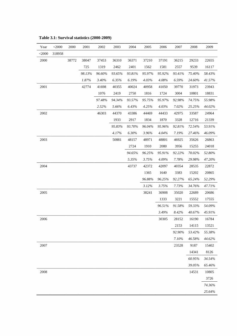
Table 3.1: Survival statistics (2000-2009)
Year <2000 2000 2001 2002 2003 2004 2005 2006 2007 2008 2009
<2000 318958
2000 38772 38047 37453 36310 36371 37210 37191 36215 29233 22655
725 1319 2462 2401 1562 1581 2557 9539 16117
98.13% 96.60% 93.65% 93.81% 95.97% 95.92% 93.41% 75.40% 58.43%
1.87% 3.40% 6.35% 6.19% 4.03% 4.08% 6.59% 24.60% 41.57%
2001 42774 41698 40355 40024 40958 41050 39770 31973 23943
1076 2419 2750 1816 1724 3004 10801 18831
97.48% 94.34% 93.57% 95.75% 95.97% 92.98% 74.75% 55.98%
2.52% 5.66% 6.43% 4.25% 4.03% 7.02% 25.25% 44.02%
2002 46303 44370 43386 44469 44433 42975 33587 24964
1933 2917 1834 1870 3328 12716 21339
95.83% 93.70% 96.04% 95.96% 92.81% 72.54% 53.91%
4.17% 6.30% 3.96% 4.04% 7.19% 27.46% 46.09%
2003 50881 48157 48971 48801 46925 35626 26863
2724 1910 2080 3956 15255 24018
94.65% 96.25% 95.91% 92.22% 70.02% 52.80%
5.35% 3.75% 4.09% 7.78% 29.98% 47.20%
2004 43737 42372 42097 40354 28535 22872
1365 1640 3383 15202 20865
96.88% 96.25% 92.27% 65.24% 52.29%
3.12% 3.75% 7.73% 34.76% 47.71%
2005 38241 36908 35020 22689 20686
1333 3221 15552 17555
96.51% 91.58% 59.33% 54.09%
3.49% 8.42% 40.67% 45.91%
2006 30305 28152 16190 16784
2153 14115 13521
92.90% 53.42% 55.38%
7.10% 46.58% 44.62%
2007 23528 9187 15402
14341 8126
60.95% 34.54%
39.05% 65.46%
2008 14531 10805
3726
74.36%
25.64%

86
Figure 3.1 Average survival rates by firm age
Figure 3.2 Average survival rates by year
89.74%
82.08% 83.74% 82.85% 81.41%78.56%
74.02%
65.69%
58.43%
0.00%
10.00%
20.00%
30.00%
40.00%
50.00%
60.00%
70.00%
80.00%
90.00%
100.00%
1 year 2 year 3 year 4 year 5 year 6 year 7 year 8 year 9 year
Surv
ival
%
Firm age
98.13% 97.06% 94.67% 93.96% 96.19% 96.08%92.58%
65.82%
56.21%
0.00%
20.00%
40.00%
60.00%
80.00%
100.00%
120.00%
2001 2002 2003 2004 2005 2006 2007 2008 2009
Surv
ival
%
Year

87
Figure 3.3 Survival rates in 2009
58.43%55.98%
53.91% 52.80% 52.29% 54.09% 55.38%
34.54%
74.36%
0.00%
10.00%
20.00%
30.00%
40.00%
50.00%
60.00%
70.00%
80.00%
2000 2001 2002 2003 2004 2005 2006 2007 2008
Surv
ival
%
Year of establishment

88
Table 3.2 presents the summary statistics of variables used in Equation (3.3). It is
interesting to see that the majority of firms in the sample (63.8%) have no political
affiliations with any level of government, and the ratio of unaffiliated firms
dramatically increases from 13.7% in 2000 to 84.4% in 2009. This could be due to the
China’s marketization reform starting from the late 1970s.
In terms of ownership, our sample is dominated by private ownership, the individual
investors and corporation entities investors occupy 46.5% and 21.2% respectively over
the period of 2000-2009. There is a dramatic decline in the proportion of state
ownership in our sample, from 22.5% in 2000 to 3.1% in 2009. A similar pattern holds
for collective firms, whose share drops from 22.9% to 4%. In contrast, the share of
individual investors increases from 21.9% to 77.3%.
Last but not least, 74.5% of firms do not export over the sample period, which
dominates out data. This ratio remains stable in the ten years. Moreover, most firms in
our sample (89.3%) do not engage in R&D.

89
Table 3.2: Descriptive statistics (2000-2009)
Variables Definition 2000-2009 2000 2009
Mean SD Mean SD Mean SD
lr_stocks ln inventories (billion RMB 2002 prices) -6.367 1.861 -6.282 1.841 -6.466 1.802
lr_sales ln sales (billion RMB 2002 prices) -3.874 1.385 -4.393 1.575 -3.531 1.237
p_capstate Proportion of capital owned by the State 0.086 0.270 0.255 0.418 0.031 0.174
p_capcoll Proportion of capital owned by collective firms 0.085 0.263 0.229 0.390 0.040 0.196
p_capcorporate Proportion of capital owned by corporations/legal entities 0.212 0.382 0.171 0.339 0.000 0.000
p_capindividual Proportion of capital owned by individuals 0.465 0.480 0.219 0.382 0.773 0.419
p_capforeign Proportion of capital owned by foreigners 0.074 0.245 0.056 0.204 0.079 0.269
no_politics No political affiliations 0.638 0.481 0.137 0.343 0.844 0.363
high_politics High political affiliations with central or provincial governments 0.044 0.205 0.085 0.279 0.015 0.123
no_exporter A dummy variable for non-exporters 0.745 0.436 0.759 0.428 0.777 0.416
lage ln firm age (based on year-of-birth) 2.157 0.874 2.443 0.928 2.243 0.646
lliquid ln [1+ratio of (current assets-current liabilities- inventories) to total assets] 0.116 0.154 0.108 0.146 0.146 0.165
neg_liquid Dummy =1 if ratio of (current assets-current liabilities- inventories) to total assets ≤ 0 0.459 0.498 0.458 0.498 0.357 0.479
lfc ln selling and distribution spending 1.052 0.859 1.205 0.941 0.933 0.774
rd_dum Dummy variable=1 if firm undertook any spending on R&D 0.107 0.310 0.119 0.324 0.073 0.260
city200 Dummy=1 for firms located in top 200 cities based on population size 0.870 0.336 0.800 0.400 0.885 0.319
t_trend Time trend (start from 2000)
N Number of observations 2,290,530 149,851 155,903
firm_id Number of firms 648,030
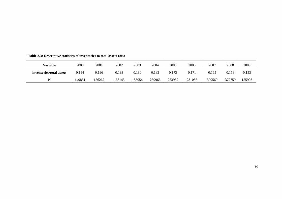
90
Table 3.3: Descriptive statistics of inventories to total assets ratio
Variable 2000 2001 2002 2003 2004 2005 2006 2007 2008 2009
inventories/total assets 0.194 0.196 0.193 0.180 0.182 0.173 0.171 0.165 0.158 0.153
N 149851 156267 168143 183054 259966 253932 281086 309569 372759 155903

91
Figure 3.4 Inventories to total assets ratio
Table 3.3 display summary statistics of inventories to total assets ratio and the number
of observations for each sample year. The number of observations ranges from a
minimum of 149,851 firms to a maximum of 372,759 firms. A decline of inventories
to total assets ratio could also be concluded during the sample period, from 19.4 in
2000 to 15.3% in 2009, which provides us a general picture of inventory reduction
among Chinese manufacturing sectors (see Figure 3.4).
0.194 0.196 0.1930.18 0.182
0.173 0.1710.165
0.158 0.153
0
0.05
0.1
0.15
0.2
0.25
2000 2001 2002 2003 2004 2005 2006 2007 2008 2009
Inven
tori
es/t
ota
l as
sets
Year

92
3.4 Estimation results and discussion
By estimating the target adjustment inventory investment model augmented with
specific firms’ characteristics, like the one presented in Equation (3.6), we report the
main results for 26 two-digit industries/industry groups in Table 3.4(a), Table 3.4(b)
and Table 3.4(c). Panel A presents the short-run dynamics, including the short-run
coefficients of lags 1 and 2 of inventory level and the speed of adjustment while panel
B contains the long-run coefficients on the determinants of target inventory level.
Generally speaking, the AR(2) and Hansen test of no second-order autocorrelation and
valid instruments cannot be rejected at 5% conventional significance levels or better,
which indicate that the estimation results are statistically sensible. Although a wide
range of explanatory variables are included in the analysis, it is unlikely to have
multicollinearity issue since the number of observations is vast and Z-values are not
low.
We begin the discussion by focusing on the short-term dynamics. Coefficients of lag1
and lag2 of inventories are significantly positive and less than 1 for most industries,
which provides evidence for the existent of partial adjustment phenomenon. The
coefficients of lag1 of inventories tend to be larger than that of lag2 for all industries
and furthermore, for some industries such as medical, metal and non-metal products,

93
the significance of inventories coefficients decreases when the lag increased, thus
indicating a loss in intensity of the adjustment path. The speed of adjustment towards
the desired level of inventories is significant for 25 out of 26 industries and on average,
Chinese firms could change about half of their deviation from target inventory level in
short-run (the average speed of adjustment is around 0.5). It is interesting to note that
the speed of adjustment is quite low for non-metal products industry, only 0.228, which
means it would take almost 2.674 years to move half-way to reach the long term goals.
It would only take about 0.64 years for firms in the leather industry to achieve the
optimal long-term inventory level, since they have the fastest adjustment speed, 0.662,
according to the results. For tobacco industry, coefficients of lag1 of inventories are
0.742, which is the second highest among all industries, and the speed of adjustment
is insignificant. These indicate that tobacco manufacturers are confronted with very
high adjustment cost so that they could not revise their outputs within a short-term
when demand change.
In terms of long-run results, the elasticity of inventory level to sales is positive and
significant for all industries but displays obvious heterogeneity among industries. The
magnitude of the coefficients provides clear evidence of the role played by inventories
4 The time it takes to achieve an elimination of 50% of the gap is calculated by: T = −
ln(2)
ln (1−δ), where 𝛿 is the
speed of adjustment. Details of the half-life convergence time is presented in appendix 3.

94
in buffering demand fluctuation, and the heterogeneity could be explained by the
variety of inventory-to-sales ratio for different industries.
The five ownership structures that we examined have a distinctive influence on firms’
inventory decisions. By setting the capital owned by Hong Kong/Macao and Taiwan
as a benchmark, we find that the proportions of capital owned by the state, collective
firms, corporations/legal entities and individual have significant negative relations
with inventory holdings. On the other hand, the foreign ownership is positively
associated with the level of inventory holdings in 6 out of 26 industries. These results
indicate that a higher proportion of domestic or mainland ownership usually related to
a lower level of inventories. In a corporate governance perspective, this could be due
to a separation of ownership and management. When focusing on the state and
individually owned firms, we find that each percent growth of state-owned ratio reduce
fewer inventory holdings when compared with that of individually owned ratio, which
means the state-owned firms tend to accumulate more inventories. This could be
explained by the facts that individually owned firms usually have a higher level of
productivity and are more likely to be financially constrained.
The coefficients of high and no political affiliation do not show completely
symmetrical patterns. The impact of high political affiliation seems to be more
widespread among industries, 20 industries are affected, compared to no political

95
affiliation, the coefficient on which is significant only for 8 industries. Generally
speaking, firms with higher level of political affiliation usually have a higher level of
inventories, which is in line with the view that a close relationship with the government
could benefit firms in better financial condition and the exposure in market
competition could motivate firms to improve their productivity. However, issues arise
in two most competitive industries and two highly monopolistic industry: it is shown
that no political affiliation would make firms in apparel and footwear industry hold
more inventories and high political affiliation has negative relation with the inventory
level in culture and water production industries.
Following literature such as Guariglia and Mateut (2010), we take the impact of firm’s
financial condition on inventory into consideration. As stated before, liquidity is
measured by the net working capital deducted by the value of inventories and the
negative liquidity is captured by the dummy named neg_liquidity. We find that firms
that are experiencing negative liquidity is associated with a significantly lower level
of inventories for more than half of the industries. This finding is consistent with the
fact that firms with bad financial condition could not afford the inventory accumulation
or even convert inventories into other kind of current assets in order to ease their
finance pressures. For industries like other mining, timber, non-metal product and
water production, the liquidity is positively related to inventory level. This indicates

96
that firms with better financial condition are able to afford the cost of inventory
accumulation and tend to have a higher level of inventory. However, for industries like
machinery & equipment, printing and textile etc., a higher liquidity ratio does not lead
to an increase in the level of inventory. This may infers that the financial condition
and inventory level is not linear related. Same as the reversed U-shape investment
curve detected by Cleary et. al. (2007), when firms are experiencing a bad financial
condition, a negative liquidity for instance, inventories tend to be seen as a source of
internal funds and firms will reduce their inventory holdings to ease financial
constraints. When the financial condition getting better and firms have enough
liquidity, the relation between liquidity and inventory becomes positive. However,
this relationship becomes negative when firms have much liquidity surplus (Baños-
Caballero et al., 2014). One possible explanation would be that when firms have
accumulated inventories to a certain level, an increase of liquidity will not lead to a
growth of inventories since the cost of holding inventories would be very high and
firms tend to do other investment so that they can get higher profits.
The result shows that dummy related to export activities is negatively related to
inventory level, which indicates that firms undertaking export activities tend to have
more inventories. This result is surprising to some extents, since, according to the
literature, exporting firms are more likely to have superior performance compared to

97
their non-exporting counterparts in terms of productivity and technology development
(Bernard et al., 2007, De Loecker, 2007). Therefore, they should enjoy a shorter
production cycle and lower inventory volume. The processing trade argument may
provide a sensible explanation. Wang and Yu (2012) state that processing trade
accounts for about 60% of Chinese export volume and processing exporters are usually
suffer low productivity (Dai et al., 2012), which offsets the productivity advantage of
undertaking export overall.
In terms of the fixed managerial cost, statistically, the rise of selling and distribution
costs seems to motivate firms stock more. This impact could be found in most
manufacturing industries in China (the tobacco industry is an exception). For this
matter of fact, we believe that the managerial fixed cost is one of the common
determinants across industries. The coefficient on city200 dummy is significant only
for six industries. This variable has a positive impact on inventories for those industries
that have a large product demand and higher inventory turnovers in the urban area,
such as apparel and footwear, culture, non-metal products, machinery and equipment
and measuring instrument. This refers that, for these industries, firms’ goal of customer
responsiveness provides motivation for having goods as near to the final consumer as
possible (Nozick and Turnquist, 2001) and locating DCs in big cities is a good choice
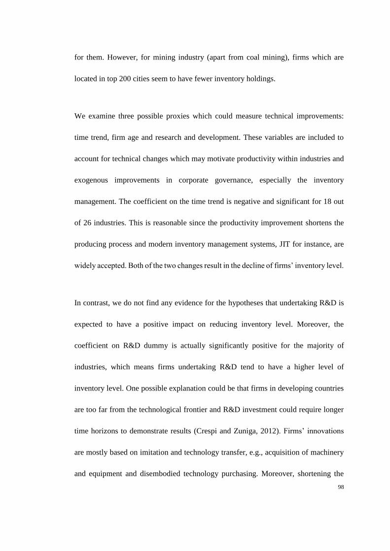
98
for them. However, for mining industry (apart from coal mining), firms which are
located in top 200 cities seem to have fewer inventory holdings.
We examine three possible proxies which could measure technical improvements:
time trend, firm age and research and development. These variables are included to
account for technical changes which may motivate productivity within industries and
exogenous improvements in corporate governance, especially the inventory
management. The coefficient on the time trend is negative and significant for 18 out
of 26 industries. This is reasonable since the productivity improvement shortens the
producing process and modern inventory management systems, JIT for instance, are
widely accepted. Both of the two changes result in the decline of firms’ inventory level.
In contrast, we do not find any evidence for the hypotheses that undertaking R&D is
expected to have a positive impact on reducing inventory level. Moreover, the
coefficient on R&D dummy is actually significantly positive for the majority of
industries, which means firms undertaking R&D tend to have a higher level of
inventory level. One possible explanation could be that firms in developing countries
are too far from the technological frontier and R&D investment could require longer
time horizons to demonstrate results (Crespi and Zuniga, 2012). Firms’ innovations
are mostly based on imitation and technology transfer, e.g., acquisition of machinery
and equipment and disembodied technology purchasing. Moreover, shortening the

99
producing process is not the priority for firms conducting R&D, and instead, firms that
have the ability to spend on R&D could be seen as financial unconstraint and, therefore,
are willing to have a higher level of inventories (Ughetto, 2008). In other words, the
R&D dummy could also be recognized as an alternative financial factor.
Firm age is found to affect inventory level significantly and positively for most
industries. However, electronic power that has a significantly negative coefficient
seems to be an exception. This is consistent with the belief that younger firms perform
their business in a more efficient way and enjoy more advanced technologies than
older firms. However, the opinion that firm would decline its inventory when become
more experienced and familiar with the market during operation is not supported by
our analysis.

100
Table 3.4a: System GMM estimation of the symmetric inventory model, China 2000-2009 (i)
Dependent
Variable:
Other
Mining
Food
Production Tobacco Textile
Apparel &
Footwear Leather Timber
Furniture
Paper-
making
lr_stocks sic10 sic14 sic16 sic17 sic18 sic19 sic20 sic21 sic22
Panel A: Short-run dynamics
L.lr_stocks 0.438*** 0.405*** 0.742*** 0.455*** 0.393*** 0.455* 0.457*** 0.463*** 0.486***
(0.018) (0.020) (0.100) (0.017) (0.015) (0.235) (0.020) (0.021) (0.015)
L2.lr_stocks 0.106*** 0.051*** 0.086* 0.073*** 0.061*** -0.116 0.104*** 0.075*** 0.110***
(0.017) (0.017) (0.046) (0.016) (0.011) (0.162) (0.015) (0.019) (0.014)
Speed of
Adjustment
0.455*** 0.544*** 0.172 0.472*** 0.546*** 0.662*** 0.439*** 0.463*** 0.405***
(0.031) (0.032) (0.115) (0.032) (0.023) (0.104) (0.031) (0.034) (0.024)
Panel B: Long-run equilibrium
lr_sales 0.418*** 0.652*** 2.406* 0.456*** 0.954*** 0.244*** 0.623*** 0.476*** 0.489***
(0.061) (0.056) (1.440) (0.042) (0.114) (0.056) (0.092) (0.072) (0.054)
p_capstate -0.245 -0.367*** 1.141 -0.273*** -0.228* -0.692*** -0.564*** -0.711*** -0.283**
(0.239) (0.104) (2.877) (0.063) (0.131) (0.235) (0.153) (0.264) (0.118)
p_capcoll -0.593** -0.293*** 1.434 -0.561*** -0.383*** -0.880*** -0.840*** -0.841*** -0.687***
(0.234) (0.086) (2.914) (0.056) (0.074) (0.095) (0.151) (0.158) (0.091)
p_capcorporate -0.415* -0.188*** 1.058 -0.460*** -0.312*** -0.665*** -0.551*** -0.558*** -0.454***
(0.227) (0.060) (2.949) (0.041) (0.046) (0.065) (0.098) (0.088) (0.082)
p_capindividual -0.451** -0.196*** 3.321 -0.517*** -0.374*** -0.846*** -0.683*** -0.727*** -0.568***
(0.224) (0.061) (3.944) (0.040) (0.044) (0.060) (0.093) (0.079) (0.079)
p_capforeign 0.241 0.035 -7.770 -0.060 -0.134*** -0.063 0.060 -0.015 0.162*
(0.279) (0.057) (9.966) (0.046) (0.042) (0.063) (0.102) (0.082) (0.093)
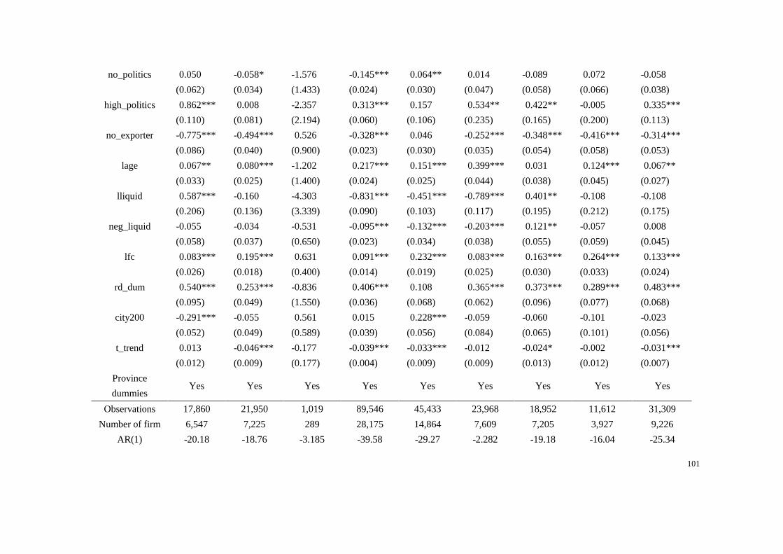
101
no_politics 0.050 -0.058* -1.576 -0.145*** 0.064** 0.014 -0.089 0.072 -0.058
(0.062) (0.034) (1.433) (0.024) (0.030) (0.047) (0.058) (0.066) (0.038)
high_politics 0.862*** 0.008 -2.357 0.313*** 0.157 0.534** 0.422** -0.005 0.335***
(0.110) (0.081) (2.194) (0.060) (0.106) (0.235) (0.165) (0.200) (0.113)
no_exporter -0.775*** -0.494*** 0.526 -0.328*** 0.046 -0.252*** -0.348*** -0.416*** -0.314***
(0.086) (0.040) (0.900) (0.023) (0.030) (0.035) (0.054) (0.058) (0.053)
lage 0.067** 0.080*** -1.202 0.217*** 0.151*** 0.399*** 0.031 0.124*** 0.067**
(0.033) (0.025) (1.400) (0.024) (0.025) (0.044) (0.038) (0.045) (0.027)
lliquid 0.587*** -0.160 -4.303 -0.831*** -0.451*** -0.789*** 0.401** -0.108 -0.108
(0.206) (0.136) (3.339) (0.090) (0.103) (0.117) (0.195) (0.212) (0.175)
neg_liquid -0.055 -0.034 -0.531 -0.095*** -0.132*** -0.203*** 0.121** -0.057 0.008
(0.058) (0.037) (0.650) (0.023) (0.034) (0.038) (0.055) (0.059) (0.045)
lfc 0.083*** 0.195*** 0.631 0.091*** 0.232*** 0.083*** 0.163*** 0.264*** 0.133***
(0.026) (0.018) (0.400) (0.014) (0.019) (0.025) (0.030) (0.033) (0.024)
rd_dum 0.540*** 0.253*** -0.836 0.406*** 0.108 0.365*** 0.373*** 0.289*** 0.483***
(0.095) (0.049) (1.550) (0.036) (0.068) (0.062) (0.096) (0.077) (0.068)
city200 -0.291*** -0.055 0.561 0.015 0.228*** -0.059 -0.060 -0.101 -0.023
(0.052) (0.049) (0.589) (0.039) (0.056) (0.084) (0.065) (0.101) (0.056)
t_trend 0.013 -0.046*** -0.177 -0.039*** -0.033*** -0.012 -0.024* -0.002 -0.031***
(0.012) (0.009) (0.177) (0.004) (0.009) (0.009) (0.013) (0.012) (0.007)
Province
dummies Yes Yes Yes Yes Yes Yes Yes Yes Yes
Observations 17,860 21,950 1,019 89,546 45,433 23,968 18,952 11,612 31,309
Number of firm 6,547 7,225 289 28,175 14,864 7,609 7,205 3,927 9,226
AR(1) -20.18 -18.76 -3.185 -39.58 -29.27 -2.282 -19.18 -16.04 -25.34
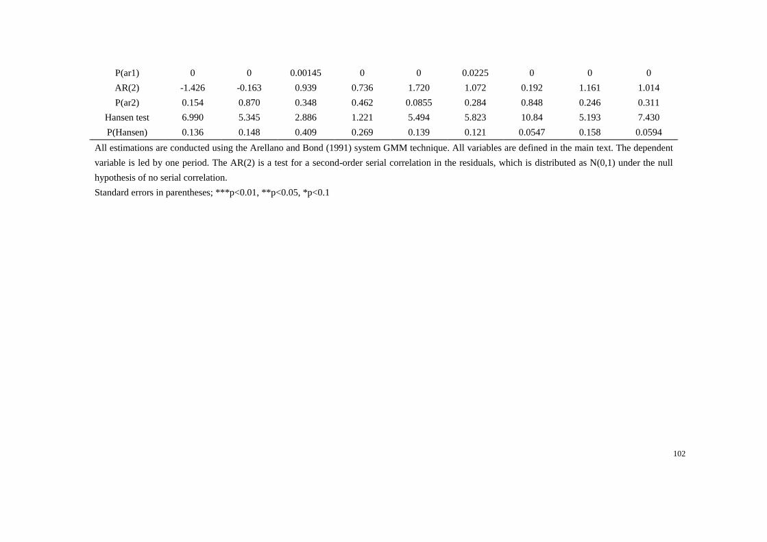
102
P(ar1) 0 0 0.00145 0 0 0.0225 0 0 0
AR(2) -1.426 -0.163 0.939 0.736 1.720 1.072 0.192 1.161 1.014
P(ar2) 0.154 0.870 0.348 0.462 0.0855 0.284 0.848 0.246 0.311
Hansen test 6.990 5.345 2.886 1.221 5.494 5.823 10.84 5.193 7.430
P(Hansen) 0.136 0.148 0.409 0.269 0.139 0.121 0.0547 0.158 0.0594
All estimations are conducted using the Arellano and Bond (1991) system GMM technique. All variables are defined in the main text. The dependent
variable is led by one period. The AR(2) is a test for a second-order serial correlation in the residuals, which is distributed as N(0,1) under the null
hypothesis of no serial correlation.
Standard errors in parentheses; ***p<0.01, **p<0.05, *p<0.1
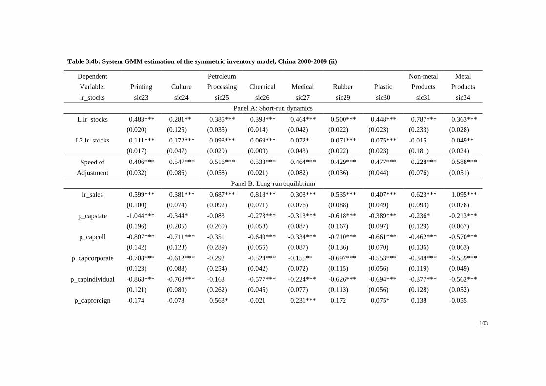
103
Table 3.4b: System GMM estimation of the symmetric inventory model, China 2000-2009 (ii)
Dependent
Variable: Printing Culture
Petroleum
Processing Chemical Medical Rubber Plastic
Non-metal
Products
Metal
Products
lr_stocks sic23 sic24 sic25 sic26 sic27 sic29 sic30 sic31 sic34
Panel A: Short-run dynamics
L.lr_stocks 0.483*** 0.281** 0.385*** 0.398*** 0.464*** 0.500*** 0.448*** 0.787*** 0.363***
(0.020) (0.125) (0.035) (0.014) (0.042) (0.022) (0.023) (0.233) (0.028)
L2.lr_stocks 0.111*** 0.172*** 0.098*** 0.069*** 0.072* 0.071*** 0.075*** -0.015 0.049**
(0.017) (0.047) (0.029) (0.009) (0.043) (0.022) (0.023) (0.181) (0.024)
Speed of
Adjustment
0.406*** 0.547*** 0.516*** 0.533*** 0.464*** 0.429*** 0.477*** 0.228*** 0.588***
(0.032) (0.086) (0.058) (0.021) (0.082) (0.036) (0.044) (0.076) (0.051)
Panel B: Long-run equilibrium
lr_sales 0.599*** 0.381*** 0.687*** 0.818*** 0.308*** 0.535*** 0.407*** 0.623*** 1.095***
(0.100) (0.074) (0.092) (0.071) (0.076) (0.088) (0.049) (0.093) (0.078)
p_capstate -1.044*** -0.344* -0.083 -0.273*** -0.313*** -0.618*** -0.389*** -0.236* -0.213***
(0.196) (0.205) (0.260) (0.058) (0.087) (0.167) (0.097) (0.129) (0.067)
p_capcoll -0.807*** -0.711*** -0.351 -0.649*** -0.334*** -0.710*** -0.661*** -0.462*** -0.570***
(0.142) (0.123) (0.289) (0.055) (0.087) (0.136) (0.070) (0.136) (0.063)
p_capcorporate -0.708*** -0.612*** -0.292 -0.524*** -0.155** -0.697*** -0.553*** -0.348*** -0.559***
(0.123) (0.088) (0.254) (0.042) (0.072) (0.115) (0.056) (0.119) (0.049)
p_capindividual -0.868*** -0.763*** -0.163 -0.577*** -0.224*** -0.626*** -0.694*** -0.377*** -0.562***
(0.121) (0.080) (0.262) (0.045) (0.077) (0.113) (0.056) (0.128) (0.052)
p_capforeign -0.174 -0.078 0.563* -0.021 0.231*** 0.172 0.075* 0.138 -0.055
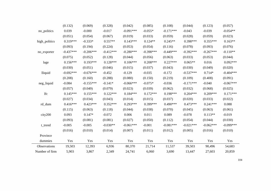
104
(0.132) (0.069) (0.328) (0.042) (0.085) (0.108) (0.044) (0.123) (0.057)
no_politics 0.039 -0.000 -0.017 -0.091*** -0.055* -0.171*** -0.043 -0.039 -0.054**
(0.051) (0.054) (0.067) (0.019) (0.033) (0.059) (0.028) (0.059) (0.023)
high_politics 0.319*** -0.333* 0.557** 0.143*** 0.124** 0.245** 0.398*** 0.355*** 0.163**
(0.093) (0.194) (0.224) (0.053) (0.054) (0.116) (0.078) (0.093) (0.076)
no_exporter -0.437*** -0.206*** -0.412*** -0.280*** -0.398*** -0.449*** -0.392*** -0.267*** -0.110**
(0.075) (0.052) (0.128) (0.044) (0.056) (0.063) (0.033) (0.053) (0.044)
lage 0.156*** 0.193*** 0.128*** 0.106*** 0.208*** 0.227*** 0.065** 0.016 0.092***
(0.030) (0.051) (0.046) (0.015) (0.037) (0.043) (0.030) (0.049) (0.020)
lliquid -0.692*** -0.676*** -0.452 -0.129 -0.035 -0.172 -0.537*** 0.714* -0.404***
(0.208) (0.160) (0.288) (0.080) (0.150) (0.219) (0.109) (0.408) (0.091)
neg_liquid -0.084 -0.155*** -0.141* -0.066*** -0.075* -0.036 -0.171*** -0.040 -0.067***
(0.057) (0.049) (0.079) (0.023) (0.039) (0.062) (0.032) (0.068) (0.025)
lfc 0.145*** 0.155*** 0.122*** 0.184*** 0.172*** 0.198*** 0.204*** 0.209*** 0.171***
(0.027) (0.034) (0.043) (0.014) (0.015) (0.037) (0.020) (0.033) (0.022)
rd_dum 0.416*** 0.423*** 0.352*** 0.293*** 0.399*** 0.490*** 0.473*** 0.241*** 0.088
(0.115) (0.063) (0.118) (0.044) (0.038) (0.070) (0.045) (0.063) (0.061)
city200 0.093 0.147* -0.072 0.006 0.011 0.089 -0.078 0.113** -0.019
(0.093) (0.081) (0.081) (0.027) (0.050) (0.112) (0.054) (0.044) (0.030)
t_trend -0.005 -0.005 -0.030** -0.061*** -0.001 -0.081*** -0.021*** -0.062*** -0.099***
(0.016) (0.010) (0.014) (0.007) (0.011) (0.012) (0.005) (0.016) (0.010)
Province
dummies Yes Yes Yes Yes Yes Yes Yes
Yes
Yes
Observations 19,503 12,393 6,936 80,370 21,714 11,537 39,503 90,496 54,683
Number of firm 5,903 3,867 2,349 24,741 6,060 3,690 13,447 27,603 20,859

105
AR(1) -20.53 -2.912 -11.12 -37.44 -20.30 -15.22 -25.68 -2.661 -26.65
P(ar1) 0 0.00359 0 0 0 0 0 0.00779 0
AR(2) -0.693 -1.354 1.825 0.355 -0.446 -1.234 0.175 0.822 0.430
P(ar2) 0.488 0.176 0.0680 0.723 0.656 0.217 0.861 0.411 0.667
Hansen test 6.245 9.475 3.120 5.499 1.648 1.551 5.316 3.020 0.206
P(Hansen) 0.182 0.0915 0.210 0.0640 0.649 0.460 0.150 0.388 0.650
All estimations are conducted using the Arellano and Bond (1991) system GMM technique. All variables are defined in the main text. The dependent
variable is led by one period. The AR(2) is a test for a second-order serial correlation in the residuals, which is distributed as N(0,1) under the null
hypothesis of no serial correlation.
Standard errors in parentheses; ***p<0.01, **p<0.05, *p<0.1
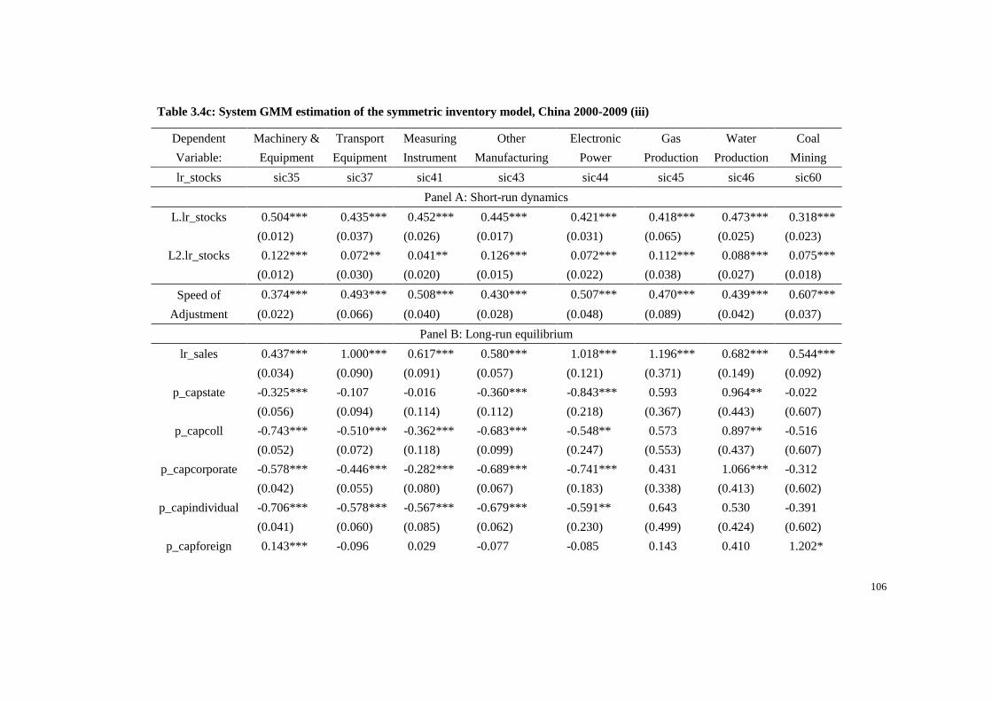
106
Table 3.4c: System GMM estimation of the symmetric inventory model, China 2000-2009 (iii)
Dependent
Variable:
Machinery &
Equipment
Transport
Equipment
Measuring
Instrument
Other
Manufacturing
Electronic
Power
Gas
Production
Water
Production
Coal
Mining
lr_stocks sic35 sic37 sic41 sic43 sic44 sic45 sic46 sic60
Panel A: Short-run dynamics
L.lr_stocks 0.504*** 0.435*** 0.452*** 0.445*** 0.421*** 0.418*** 0.473*** 0.318***
(0.012) (0.037) (0.026) (0.017) (0.031) (0.065) (0.025) (0.023)
L2.lr_stocks 0.122*** 0.072** 0.041** 0.126*** 0.072*** 0.112*** 0.088*** 0.075***
(0.012) (0.030) (0.020) (0.015) (0.022) (0.038) (0.027) (0.018)
Speed of
Adjustment
0.374*** 0.493*** 0.508*** 0.430*** 0.507*** 0.470*** 0.439*** 0.607***
(0.022) (0.066) (0.040) (0.028) (0.048) (0.089) (0.042) (0.037)
Panel B: Long-run equilibrium
lr_sales 0.437*** 1.000*** 0.617*** 0.580*** 1.018*** 1.196*** 0.682*** 0.544***
(0.034) (0.090) (0.091) (0.057) (0.121) (0.371) (0.149) (0.092)
p_capstate -0.325*** -0.107 -0.016 -0.360*** -0.843*** 0.593 0.964** -0.022
(0.056) (0.094) (0.114) (0.112) (0.218) (0.367) (0.443) (0.607)
p_capcoll -0.743*** -0.510*** -0.362*** -0.683*** -0.548** 0.573 0.897** -0.516
(0.052) (0.072) (0.118) (0.099) (0.247) (0.553) (0.437) (0.607)
p_capcorporate -0.578*** -0.446*** -0.282*** -0.689*** -0.741*** 0.431 1.066*** -0.312
(0.042) (0.055) (0.080) (0.067) (0.183) (0.338) (0.413) (0.602)
p_capindividual -0.706*** -0.578*** -0.567*** -0.679*** -0.591** 0.643 0.530 -0.391
(0.041) (0.060) (0.085) (0.062) (0.230) (0.499) (0.424) (0.602)
p_capforeign 0.143*** -0.096 0.029 -0.077 -0.085 0.143 0.410 1.202*

107
(0.041) (0.064) (0.085) (0.067) (0.198) (0.317) (0.647) (0.636)
no_politics -0.088*** -0.054* 0.017 -0.061 0.069 -0.046 0.036 0.001
(0.020) (0.029) (0.043) (0.044) (0.070) (0.172) (0.133) (0.054)
high_politics 0.405*** 0.195*** 0.250*** 0.453*** -0.205 -0.448 -0.406* 1.042***
(0.035) (0.063) (0.084) (0.095) (0.182) (0.512) (0.237) (0.172)
no_exporter -0.324*** -0.124** -0.230*** -0.095** -0.093 0.164 0.140 0.033
(0.022) (0.061) (0.057) (0.039) (0.147) (0.548) (0.215) (0.117)
lage 0.164*** 0.161*** 0.166*** 0.284*** -0.306*** -0.100 0.042 0.110***
(0.020) (0.030) (0.031) (0.034) (0.046) (0.185) (0.090) (0.026)
lliquid -0.441*** -0.386*** -0.735*** -0.462*** -0.038 -1.585*** 0.707** 0.254
(0.074) (0.110) (0.149) (0.149) (0.298) (0.579) (0.331) (0.203)
neg_liquid -0.089*** -0.040 -0.203*** -0.203*** 0.159*** -0.353** 0.074 0.007
(0.021) (0.031) (0.046) (0.049) (0.053) (0.151) (0.075) (0.053)
lfc 0.278*** 0.200*** 0.252*** 0.190*** 0.055* 0.249*** 0.092*** 0.138***
(0.013) (0.018) (0.029) (0.026) (0.034) (0.076) (0.029) (0.023)
rd_dum 0.567*** 0.169** 0.366*** 0.528*** -0.319** -0.483 0.183 0.527***
(0.024) (0.081) (0.072) (0.052) (0.156) (0.360) (0.282) (0.113)
city200 0.154*** 0.036 0.184* 0.053 0.030 0.052 0.103 -0.025
(0.030) (0.045) (0.100) (0.073) (0.084) (0.253) (0.120) (0.046)
t_trend -0.036*** -0.071*** -0.027*** -0.019** -0.054*** -0.138*** 0.017 -0.073***
(0.004) (0.011) (0.007) (0.008) (0.017) (0.053) (0.021) (0.012)
Province
dummies Yes Yes Yes Yes Yes Yes Yes
Yes
Observations 148,039 44,393 14,754 25,924 15,860 1,864 9,062 16,248
Number of firm 49,026 13,999 6,556 9,354 4,473 535 2,293 5,521
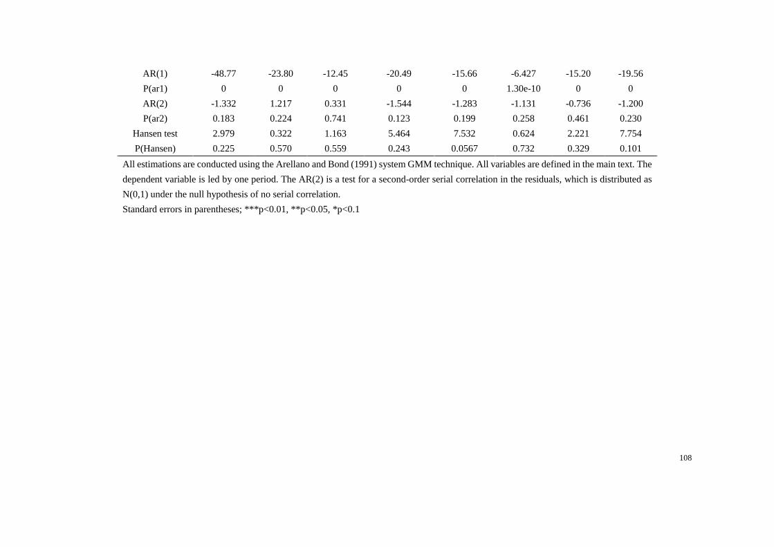
108
AR(1) -48.77 -23.80 -12.45 -20.49 -15.66 -6.427 -15.20 -19.56
P(ar1) 0 0 0 0 0 1.30e-10 0 0
AR(2) -1.332 1.217 0.331 -1.544 -1.283 -1.131 -0.736 -1.200
P(ar2) 0.183 0.224 0.741 0.123 0.199 0.258 0.461 0.230
Hansen test 2.979 0.322 1.163 5.464 7.532 0.624 2.221 7.754
P(Hansen) 0.225 0.570 0.559 0.243 0.0567 0.732 0.329 0.101
All estimations are conducted using the Arellano and Bond (1991) system GMM technique. All variables are defined in the main text. The
dependent variable is led by one period. The AR(2) is a test for a second-order serial correlation in the residuals, which is distributed as
N(0,1) under the null hypothesis of no serial correlation.
Standard errors in parentheses; ***p<0.01, **p<0.05, *p<0.1

109
3.5 Conclusions
We have exploited a large unbalanced panel datasets of Chinese manufacturing firms
observed over the period 2000-2009 to assess how certain factors determines the long-
run target inventory level and whether the inventory dynamics differ among industries.
When estimating the equation, we favour the system GMM estimator because of its
ability to capture firm-level fixed effects and to deal with the endogeneity of regressors.
Besides the sales and liquidity variables, we include in the inventory adjustment model
several other specific variables such as firms’ political affiliation and ownership,
geographic location, in order to make a more comprehensive long-run inventory
analysis. Also, the estimations are separate for each industry to allow for heterogeneity
in unobserved industry-specific characteristics.
Generally speaking, in terms of short-run dynamics, a partial adjustment mechanism
has been proved. The speeds of adjustment toward the desired level of inventories are
significantly positive, and they are various among different industries from 0.228 to
0.662. From the long-run perspectives, sales, ownership structure and managerial fixed
cost are important indicators of the target inventory level among all industries.
Heterogeneous exists on the effect of political affiliation and the coefficients of high
and no political affiliation do not show completely symmetrical patterns. Neither
110
export behaviour nor R&D spending is found to impact strongly consistent with our
expectations, possibly due to the facts of the large volume of processing trade and long
distance from the technological frontier in the Chinese economy. From 2000 to 2009,
18 out of 26 industries have reduced their long run target level of inventory. Moreover,
in line with previous literature, younger firms perform with a lower level of inventories
with more advanced technologies than older firms and the U-shaped inventory-
financial performance relation is detected for most of the industries.

111
Chapter 4. Asymmetric inventory
adjustment: new evidence from dynamic
panel threshold model
112
Chapter 4. Asymmetric inventory adjustment: new
evidence from dynamic panel threshold model
4.1 Introduction
In the previous chapter, we document evidence in favour of firm level inventory short-
run dynamic and long-run target adjustment pattern. However, an important limitation
of this analysis, same as recent empirical research in this field of study, is that we
assume symmetry in the mechanism of adjustment, such that firms adjust at the same
rate toward desired inventory level regardless of exogenous parameters that affect the
macro business environment. Consequently, we did not allow for a possibility that
firms employ differential adjustment policy toward their optimal inventory structure
following macro business cycle fluctuation.
Research on inventory investment has been focused on its role in business cycles. Due
to its procyclical and persistent properties, inventory investment is found to be a
leading indicator of business cycles. Inventory research at the macro-level provides a
huge amount of evidence that questions the motivations of holding inventory at the
firm level. For example, if firms hold inventory to smooth production, then why is it
observed at the macro-level that production is more volatile than sales? The related

113
puzzle is why inventory investment shows a strong procyclical and persistent
movement. The discrepancy between inventory theories and stylised empirical
evidence has worried economists for decades. There might be some factors missing in
the existing literature on inventory investment. For instance, the impact of the volatility
of stochastic variables on inventory investment is hardly discussed.
A non-linear model of investment behaviour incorporating time-varying adjustment
speeds with threshold effects is estimated for the UK manufacturing sector, which
suggests that uncertainty has a large and significant effect on both steady state levels
and rates of adjustment (Price, 1996). Bo (2000) takes the volatility of sales into
consideration and examines the relationship between demand uncertainty and
inventory investment based on the accelerator buffer stock inventory model. By
invovling a panel of Dutch listed firms in the period 1984-1996, it is found that the
estimated coefficient of the speed parameter of adjusting inventories increases vastly
when the volatility of sales is used as the proxy for unexpected sales in the inventory
adjustment equation.
This chapter aims at filling this gap in the literature by developing a more
comprehensive empirical approach, allowing for an asymmetric adjustment
mechanism. The concept of asymmetry implies that the cost of adjusting to a higher
target level are not necessarily marginally equivalent to the cost of adjusting to a lower

114
target level (Escribanao and Pfann, 1998). In particular, we propose a dynamic panel
threshold model of inventory (an industry-specific business cycle dummy is employed
as a transition variable), allowing for asymmetries in the mechanism of adjustment of
firms in different macro business regimes associated with differential adjustment
speed and target. Our model entertains a possibility that firms not only adjust at
heterogeneous speed in short-run dynamics but also adjust toward heterogeneous
inventory targets in the long-run. To illustrate the advantage of our approach, consider
a dynamic setting in which a firm faces different costs of inventory adjustment
according to its characteristics. Rather than having a unique inventory target, the firm
may have a target range within which allows its inventory level to fluctuate.
The structure of this chapter is as follows. Section 2 describes the empirical
methodology to construct asymmetric inventory adjustment model with the descriptive
statistics. Section 3 illustrates the results of our estimation while section 4 discusses
the results and concludes the chapter.
115
4.2 Asymmetric inventory adjustment analysis
4.2.1 Theoretical backgrounds
In quadratic-cost models, the optimal behaviour is based on balancing the gains from
production smoothing with the costs of deviating from some "target" level of
inventories. The models of Arrow et al. (1958) remind us that optimal production and
inventory decisions balance three margins: the benefits of production smoothing, the
costs of holding inventories, and the costs incurred if inventories are too low to meet
demand and a stockout occurs.
Differences in holding and stockout costs make it optimal for a firm to replenish
inventories following a positive demand surprise, a shock that lowers inventories and
increases the probability of experiencing a stockout, at a different speed than it reduces
output following unexpectedly low sales, a shock that increases inventory holding
costs. In particular, the difference between holding and stockout costs causes firms'
production decisions to depend on whether or not shocks push inventories above or
below desired levels.

116
4.2.2 Dynamic threshold model of inventory
Reminded that we define the symmetric adjustment model of inventory as a variant of
Error-correction model (Guariglia and Mateut, 2006), and the partial adjustment
process is written as:
∆𝐼𝑖𝑡 = 𝐼𝑖𝑡 − 𝐼𝑖,𝑡−1 = 𝛿(𝐼𝑖𝑡∗ − 𝐼𝑖,𝑡−1) + 𝑣𝑖𝑡 (4.1)
Denoting the logarithm of the actual and target level of inventories of firm i at time
t with itI and *itI , respectively. indicates the speed of adjustment that
measures how fast firms move towards their target inventory level.
The target inventory level ( *itI ) is then determined by a set of firms’ characteristics
such as sales, age, liquidity, etc.:
𝐼𝑖𝑡∗ = 𝛽′𝑋𝑖𝑡 (4.2)
To estimate the two equations, we employ the one-stage procedure (Flannery and
Rangan, 2006, Ozkan, 2001) and yields:
∆𝐼𝑖𝑡 = 𝛿(𝛽′𝑋𝑖𝑡 − 𝐼𝑖,𝑡−1) + 𝑣𝑖𝑡 = 𝛿𝛽′𝑋𝑖𝑡 − 𝛿𝐼𝑖,𝑡−1 + 𝑣𝑖𝑡

117
𝐼𝑖𝑡 = (1 − δ)𝐼𝑖,𝑡−1 + 𝛿𝛽′𝑋𝑖𝑡 + 𝑣𝑖𝑡
𝐼𝑖𝑡 = 𝜑𝐼𝑖,𝑡−1 + 𝜋′𝑋𝑖𝑡 + 𝑣𝑖𝑡 (4.3)
Where 𝜑 = 1 − 𝛿 and 𝜋 = 𝛿𝛽.
Testing the target adjustment model using equation (4.3) assumes that firms undertake
inventory adjustment in a symmetric fashion. In order to analyse the asymmetric
adjustment behaviour, we develop the regime-switching dynamic threshold model:
𝐼𝑖𝑡 = (𝜑1𝐼𝑖,𝑡−1 + 𝜋1′ 𝑋𝑖𝑡) + [(𝜑2 − 𝜑1)𝐼𝑖,𝑡−1 + (𝜋2 − 𝜋1)′𝑋𝑖𝑡]1{𝑞<𝑐} + 𝑣𝑖𝑡 (4.4)
Where 1{.} is an indicator function taking the value 1 if the event is true and 0
otherwise. Equation (4.4) represents an important extension of the linear partial
adjustment model, equation (4.3). It allows for short-run asymmetries (𝜑1 ≠ 𝜑2), as
well as long-run asymmetries in the target leverage relationship (𝜋1 ≠ 𝜋2) ,
conditional on the exogenous regime-switching transition variable, itq , and the
threshold parameter, c .

118
4.2.3 Regime-switching transition variable
In this section, we examine a number of potential reasons why we choose the industry-
specific business cycle as the transition variable, in our regime-switching framework,
equation (4.4). Our discussion is motivated by some recent empirical studies
investigating the influence of recessions on firm performance.
It is commonly accepted that during recessions, financial institutions tend to tight their
lending requirement, which dramatically change the firms’ ability to create new lines
of credit, dry up the flow of money and slow economic growth. Other shocks such as
demand decreasing and risk rising are other concerns.
4.2.3.1 Credit supply shock channel and its impact on real economy
Much of the narrative on the financial crisis has focused on the impact of a credit
supply shock: Tong and Wei (2008) propose a methodological framework to study the
underlying mechanisms by which a financial-sector crisis may affect the real sector
and apply it to the case of the most recent financial crisis. In particular, they quantify
the importance of tightening credit supply and deterioration of consumer confidence
in non-financial firms by comparing their impact on the firms’ share price. The results
show that both channels are at work, but credit supply constraints appear to be more

119
quantitatively significant in explaining cross-firm differences in the magnitude of
share price declines.
Ivashina and Scharfstein (2010) explain the decline of bank loans after the crisis from
both of demand and supply side. From the demand side, due to the recession, firms
usually slow down their expansion plan and limit their investment projects and,
therefore, the need for external finance declines. From the supply side, the amount of
funds that banks are willing to lend also decrease since banks find it difficult to get
deposits.
Campello et al. (2010) analyse firms’ investment policies during the financial crisis,
in order to test the impact of credit shock. The authors undertake a survey-based
measure of financial constraints which engaged 1050 Chief Financial Officers (CFOs)
in the US, Europe and Asia. In their study, it is said that during the crisis, financially
constrained firms cut more investment than their financially unconstrained
counterparts. For cash accumulation aspect, this paper point out that financially
constrained firms have to reduce their cash accumulations during the crisis and
decrease their planned dividend payout but this behaviour among financially
unconstrained firms is not significant. However, Duchin et al. (2010) point out that
informational asymmetry could lead to a problem which may influence the reliability
of these results. More specifically, it is possible that some of the questions in the survey
120
were misunderstood or otherwise produce noisy measures of the desired variables of
interest. In addition, when interpreting field studies, we need to consider that market
participants do not necessarily have to understand the reason they do in order to make
optimal decisions. Therefore, Duchin et al. (2010) introduce archival data in order to
fill this gap and provide a similar conclusion to the prior one.
Tong and Wei (2010) expand this topic by analysing the impact of foreign investment
on financial crisis transmission from the western market to other parts of the world. It
is said that the impact of foreign investment is not uniform. In some countries, local
firms obtain a relatively large fraction of their funding from foreign banks and other
pools of liquid capital. However, the funds which arrive quickly also depart quickly
and these firms suffered the most in the crisis. In contrast, other countries in which
investment tend to be direct, and thus sticky, were less affected.
4.2.3.2 Other transmission channels
A number of other papers have challenged the credit supply shock channel by
analysing other possible transmission channels. Using accounting data for 7722 non-
financial firms in 42 countries, Claessens et al. (2012) examine how the 2007-2009
crisis affected firm performance, especially sales, profits, and capital expenditure, and
how various transmission channels propagated shocks across borders. They employ a

121
framework to distinguish the impact of three possible channels: a financial channel
(the effect of the credit shock), a domestic demand channel (the effect of demand
decreasing), and a trade channel (the effect of a decreased international trade volume).
It is believed that firstly, if a reduction of available credit plays an important role for
firms, it should be reflected in the performance of those firms that rely more on
external finance for investment and working capital. Similarly, if the trade channel is
important, it should be reflected in a relatively worse performance of those firms that
rely more heavily on exports. Finally, if the crisis triggered a negative domestic
demand shock, it should be reflected in a relatively worse performance of those firms
that are more demand sensitive. The results show that the crisis had a more severe
negative impact on firms with greater sensitivity to demand and trade, particularly in
countries that are more open to trade. However, the financial openness appears to have
made limited differences. In other words, the trade and demand channels are the most
important. It is also shown that the trade channel played a significant role in the spill-
over of crisis while the evidence for the role of the financial channel is considerably
weaker.
Kahle and Stulz (2011) point out that, despite the credit supply shock, the crisis also
reduced demand for goods and increased risk. Therefore, they explore the impact of
the financial crisis on financial and investment policies. They believe that if the bank

122
credit supply shock were the dominant shock, the more bank-dependent firms should
have lower net debt issuance, a greater decrease in cash holdings, an increase in net
equity issuance and a greater drop in capital expenditures than less bank-dependent
firms. However, their results show that the credit supply shock cannot explain
important features of the financial and investment policies of industrial firms. More
specifically, the net equity issuance of small firms and unrated firms is abnormally low
throughout the crisis. Moreover, firms that are more bank-dependent before the crisis
tend to increase their cash holdings rather than use them to mitigate the impact of the
increased risk associated with the credit supply shock and do not reduce their capital
expenditures more than other firms during the crisis. The authors then show evidence
which is strongly supportive of theories that emphasize the importance of collateral
and corporate net worth in financing and investment policies, as firms with stronger
balance sheets reduce capital expenditures less during the crisis.
4.2.3.3 Macroeconomic movements in Chinese market
Over the past several years, China has enjoyed one of the world's fastest growing
economies and has been a major contributor to world economic growth. However, the
recent global financial crisis threatens to significantly slow China's economy. Liu
(2009) investigates how China is affected by the global economic slowdown by
analysing business cycle co-movements through time between China and the USA, the

123
EU and Japan (G-3 economies). It appears that business movement in China is quite
correlated with that in the USA in the 1980s, but it is not correlated with economic
fluctuations in the EU and Japan. Interestingly, the correlation coefficients between
China and the G-3 declined in the 1990s, suggesting that China was moving on its own
path of economic growth independently from the G-3 economies. However, the
correlation with the USA and Japan has become highly positive since the 2000s. In
contrast, the correlation between China and the EU was still negative over the post-
2000 period. The divergence between China and the EU was probably a result of the
weak economic performance in the EU during this period. For the G-3 economies as a
whole, the correlation coefficient was 0.23 in the 2000s, higher than the correlation
coefficients in the 1980s and the 1990s. These simple business cycle synchronisation
measures suggest that there is an increased degree of economic linkage between China
and the G-3 economies.
When focusing on the 2007-2009 financial crisis, N’Diaye et al. (2010), using a
structural macroeconomic model, estimate that a 1-percent slowdown in the G-3
economies is likely to cause more than 2-percent growth decline in emerging Asia
markets. According to Morrison (2009), the value of Shanghai Stock Exchange
Composite Index has decreased more than 67% from December 31, 2007, to December
31, 2008. China’s trade and FDI have experienced a dramatically negative impact

124
during the crisis. For example, China’s exports and imports in February 2009 were
down 25.7% and 24.1%, respectively on a year-on-year basis. The level of FDI flows
to China has declined in each of the seven months (November 2008-April 2009) on a
year-on-year basis as well. A high unemployment rate was recorded during the crisis,
and 20 million migrant workers were estimated to lose their jobs in 2008 because of
the global economic slowdown.
There seems to be a lack of research focusing on the real effect of the financial crisis
on the firms’ inventory investment decisions. Most of these studies concentrate on
Chinese market are conducted based on small samples and focus only on the effects of
financial constraints on fixed investment, with the exception of Guariglia et al. (2011)
who study the effects of financial constraints on firms’ asset growth in China. Study
based on inventory investment is motivated by the fact that inventory investment plays
an important role in the explanation of business cycle. Despite its small magnitude
relative to total production, inventory investment typically accounts for a significant
proportion of the reduction in GDP during recession. Since they can be converted into
cash rapidly with a low adjustment cost, inventories are likely to be much more
sensitive to financial variables when compared with fixed investment. Moreover,
according to the data that we have collected so far, the inventory also place an
important role in the Chinese market. It shows that inventories (defined as the sum of
125
finished goods and work-in-process inventories) represent 20% of firms’ total assets
on average, and are about 22% of sales in terms of value. Therefore, it is crucial to
have a better understanding of the inventory investment behaviour in China when firms
confront different business environment.
4.2.3.4 Recessions and inventory investment
Sangalli (2013) seems to be the first study that explores how firms adjust their
inventories during recessionary periods. Involving three large unbalanced panels of
Italian manufacturing firms observed over the period 1991–2009, it is claimed a
significant recessionary effect during the Nineties, accounting for inventories being
more sensitive to financial frictions during the main recessionary peaks, 1993 and 1996.
The result is not confirmed by the most recent estimates, especially the ones referring
to the 2008–2009 recessionary shock. Firms are found to rely on inventory
decumulation to a lesser extent compared to the past, to generate internal financing.
More specifically, disinvestments in working capital are found to represent, as a matter
of fact, one of the main drivers adopted to ease liquidity tensions: a negative and
strongly significant relationship with inventory investment is detected, after
controlling for short-run liquidity constraints at firm level. By contrast, only a weak
negative relationship is established with fixed capital during the same recessionary
period. Although this study only focuses on the link between inventory investments
126
and financial constraint in the Italian market, it still sheds some lights on our research
in this chapter.
4.2.4 Description of business cycle dummy and summary
statistics
In our study, the business cycle dummy is established according to the difference
between the real sales (Sreal) and the expected sales’ trend (Strend). In other words, the
business cycle dummy equals one (down regime) if the Sreal in a specific industry is
less than or equal to Strend and equals zero (up regime) otherwise.
The Christiano and Fitzgerald (2003)’s band-pass filter is used in order to separate the
cyclical components (Scyclical) from the time series (Sreal). The trend component (Strend)
is calculated by the difference: Strend = Sreal − Scyclical. The finite-length CF band-pass
filter places two important restrictions: First, it is restricted to be a linear filter. Second,
the time series is assumed to be a random-walk process5. Although in finite samples,
it is not possible to exactly satisfy the conditions that a filter must fulfil to perfectly
separate out the specified stochastic cycles; the expansive filter literature reflects the
5 This assumption is quoted from the Stata manual, however, according to Christinano and Fitzgerald (2003), it is
imposed on the filtered (cyclical) component of the time series, rather than the raw time series. The raw time series
should be a covariance-stationary process, possibly with non-zero mean and a deterministic trend, or it can contain
a unit root.

127
trade-offs involved in choosing a finite-length filter to separate out the specified
stochastic cycles. Burns and Mitchell (1946) define ‘oscillations in business data with
recurring periods between 1.5 and 8 years to be business-cycle fluctuations’. And
therefore, we use this commonly accepted definition.
Taking regional heterogeneity into consideration, aggregate, region-level and
province-level business cycle dummies are generated for each industry. Figure 4.1 and
Figure 4.2 describe the number of firms by region and province respectively.
Accordingly, the number of firms that are located in the three regions is not equal. 71%
of firms are located in the coastal past of China, which accounts for the majority of our
dataset. Firms that are located in the central and western part of China only stand for
17% and 12% of the whole sample respectively. More specifically, Jiangsu province
seems to have the largest number of enterprises followed by Zhejiang and Guangdong.
Provinces that are located in the Western part of China tend to have few manufacture
firms (Table 4.1 provides the description of region and province code).
Table 4.2 presents the summary statistics showing the frequencies of the three levels
of business cycle dummy from 2000 to 2009. The province-level dummy has a smaller
number of observations since we could not generate the expected sales’ trends for
some industries due to the discontinuous data in certain provinces (e.g. Hainan and
Tibet). According to the table, the proportion of the firms that fall into down regime

128
peaks in 2005 and 2009, which means most of the Chinese manufacturers have
experienced bad business environment during this two periods. This could be due to
the impacts of Asia economic crisis started from 2003 and the recent global financial
crisis which began at the end of 2007.
However, the distributions of the three dummy vary during the research period. More
specifically, the aggregative dummy is the most concentrated one, and the province-
level dummy seems to be the most scattered (see Figure 4.3). This could be due to the
fact that the business environment shocks affect the firms’ performance in different
time across the country. Therefore, the province-level business cycle dummy is used
in the following analysis in order to take this factor into consideration.

129
Figure 4.1 Number of firms by region
Figure 4.2 Number of firms by province
Coast, 458088,
71%
Centre, 113500,
17%
West, 76583, 12%
0.00%
2.00%
4.00%
6.00%
8.00%
10.00%
12.00%
14.00%
16.00%
0
10000
20000
30000
40000
50000
60000
70000
80000
90000
100000
11121314152122233132333435363741424344454650515253546162636465
Per
centa
ge
Num
ber
of
firm
s
Province code
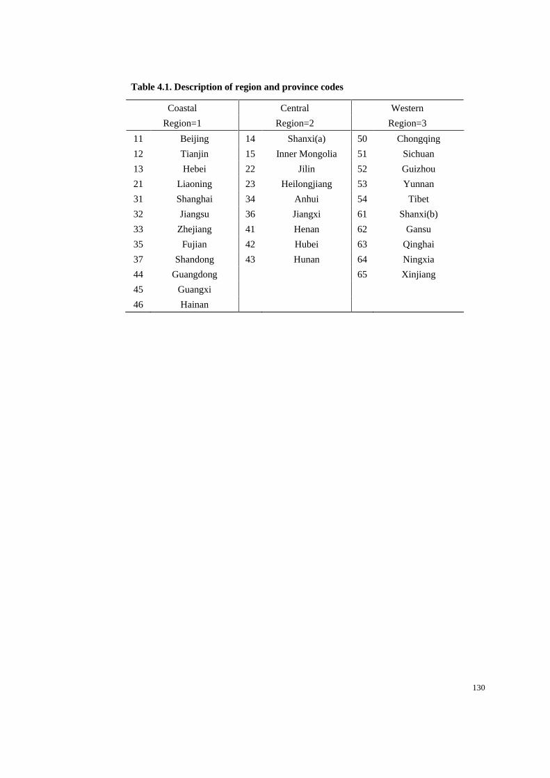
130
Table 4.1. Description of region and province codes
Coastal Central Western
Region=1 Region=2 Region=3
11 Beijing 14 Shanxi(a) 50 Chongqing
12 Tianjin 15 Inner Mongolia 51 Sichuan
13 Hebei 22 Jilin 52 Guizhou
21 Liaoning 23 Heilongjiang 53 Yunnan
31 Shanghai 34 Anhui 54 Tibet
32 Jiangsu 36 Jiangxi 61 Shanxi(b)
33 Zhejiang 41 Henan 62 Gansu
35 Fujian 42 Hubei 63 Qinghai
37 Shandong 43 Hunan 64 Ningxia
44 Guangdong 65 Xinjiang
45 Guangxi
46 Hainan

131
Table 4.2: Frequencies of the business cycle dummy
Aggregative
2000 2001 2002 2003 2004 2005 2006 2007 2008 2009 Total
0 129,298 126,380 119,630 57,964 11,710 0 19,654 262,093 314,174 0 1,040,903
(up regime) (99.76) (93.12) (81.54) (37.19) (5.28) (0.00) (8.22) (99.81) (100.00) (0.00) (53.30)
1 312 9,332 27,080 97,883 209,973 216,075 219,483 510 0 131,496 912,144
(down regime) (0.24) (6.88) (18.46) (62.81) (94.72) (100.00) (91.78) (0.19) (0.00) (100.00) (46.70)
Total 129,610 135,712 146,710 155,847 221,683 216,075 239,137 262,603 314,174 131,496 1,953,047
(100.00) (100.00) (100.00) (100.00) (100.00) (100.00) (100.00) (100.00) (100.00) (100.00) (100.00)
Region-level
2000 2001 2002 2003 2004 2005 2006 2007 2008 2009 Total
0 127,206 123,968 110,301 51,925 11,544 471 15,113 259,874 314,174 0 1,014,576
(up regime) (98.15) (91.35) (75.18) (33.32) (5.21) (0.22) (6.32) (98.96) (100.00) (0.00) (51.95)
1 2,404 11,744 36,409 103,922 210,139 215,604 224,024 2,729 0 131,496 938,471
(down regime) (1.85) (8.65) (24.82) (66.68) (94.79) (99.78) (93.68) (1.04) (0.00) (100.00) (48.05)
Total 129,610 135,712 146,710 155,847 221,683 216,075 239,137 262,603 314,174 131,496 1,953,047
(100.00) (100.00) (100.00) (100.00) (100.00) (100.00) (100.00) (100.00) (100.00) (100.00) (100.00)
Province-level
2000 2001 2002 2003 2004 2005 2006 2007 2008 2009 Total
0 114,658 117,173 101,233 70,200 51,759 10,737 34,507 249,385 307,140 1,449 1,008,241
(up regime) (88.51) (86.35) (69.01) (45.06) (23.35) (4.97) (14.43) (94.97) (97.77) (1.10) (54.19)
1 14,885 18,516 45,452 85,584 169,919 205,329 204,619 13,207 7,020 130,043 844,574
(down regime) (11.49) (13.65) (30.99) (54.94) (76.65) (95.03) (85.57) (5.03) (2.23) (98.90) (45.81)
Total 129,543 135,689 146,685 155,784 221,678 216,066 239,126 262,592 314,160 131,492 1,952,815
(100.00) (100.00) (100.00) (100.00) (100.00) (100.00) (100.00) (100.00) (100.00) (100.00) (100.00)
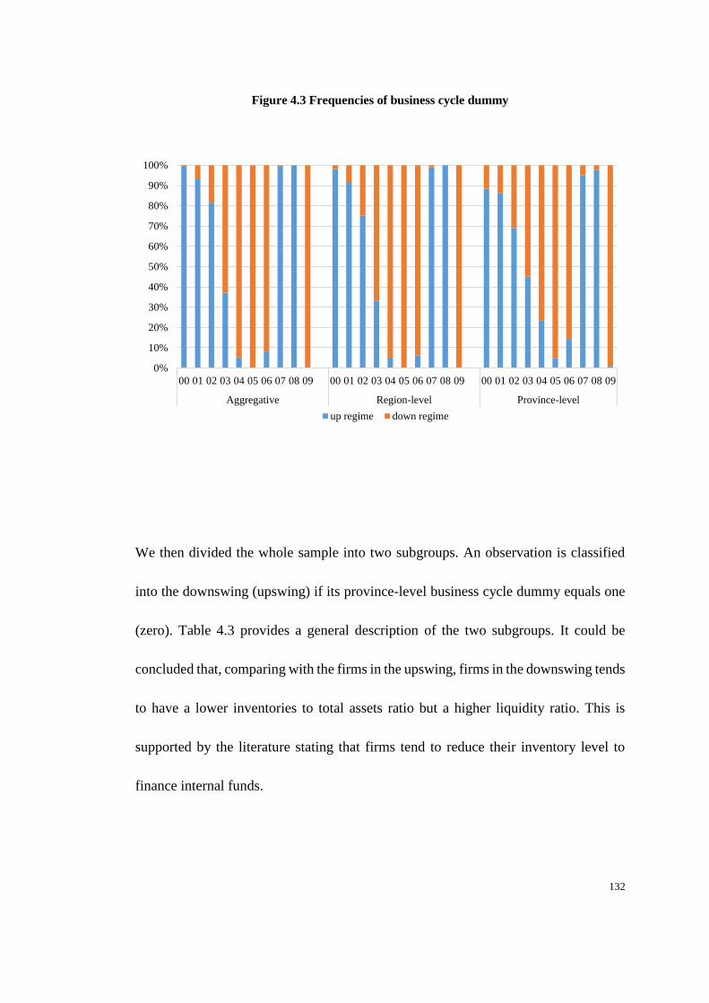
132
Figure 4.3 Frequencies of business cycle dummy
We then divided the whole sample into two subgroups. An observation is classified
into the downswing (upswing) if its province-level business cycle dummy equals one
(zero). Table 4.3 provides a general description of the two subgroups. It could be
concluded that, comparing with the firms in the upswing, firms in the downswing tends
to have a lower inventories to total assets ratio but a higher liquidity ratio. This is
supported by the literature stating that firms tend to reduce their inventory level to
finance internal funds.
0%
10%
20%
30%
40%
50%
60%
70%
80%
90%
100%
00 01 02 03 04 05 06 07 08 09 00 01 02 03 04 05 06 07 08 09 00 01 02 03 04 05 06 07 08 09
Aggregative Region-level Province-level
up regime down regime

133
Besides, firms with a higher percentage of state, collective sector and corporate
ownership are more likely to be classified into the upswing. In contrast, a higher
proportion of individual and foreign ownership may refer to a higher possibility to be
in the downswing. A high political affiliation tends to help firms get rid of the
downswing business cycle. But, surprisingly, the average age of firms in the
downswing is younger than that of firms in the upswing.
Finally, firms in the downswing are more likely to be exporters and located in big cities.
This could be due to the fact that exporters may experience international economic
shocks frequently, and firms in big cities are more likely influenced by severe
competitions.
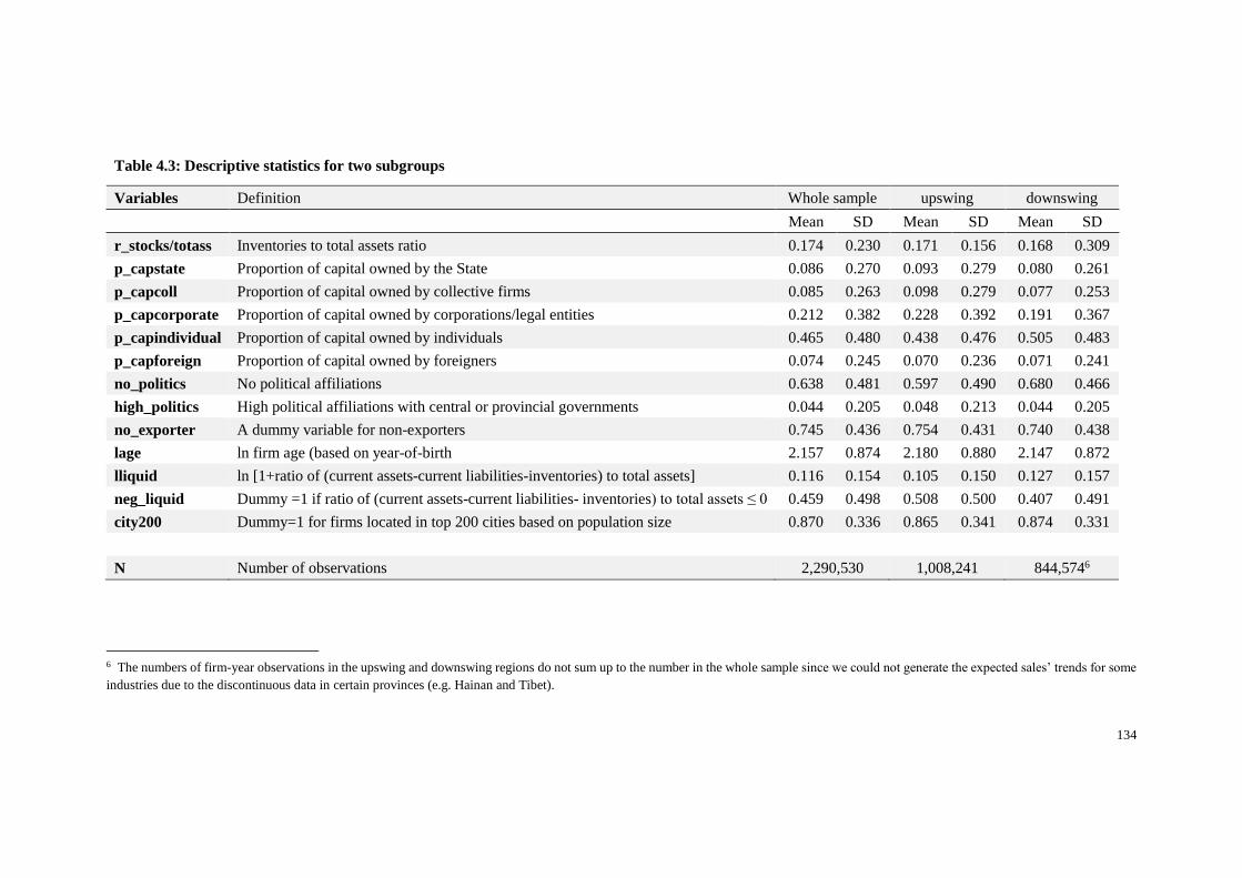
134
Table 4.3: Descriptive statistics for two subgroups
Variables Definition Whole sample upswing downswing
Mean SD Mean SD Mean SD
r_stocks/totass Inventories to total assets ratio 0.174 0.230 0.171 0.156 0.168 0.309
p_capstate Proportion of capital owned by the State 0.086 0.270 0.093 0.279 0.080 0.261
p_capcoll Proportion of capital owned by collective firms 0.085 0.263 0.098 0.279 0.077 0.253
p_capcorporate Proportion of capital owned by corporations/legal entities 0.212 0.382 0.228 0.392 0.191 0.367
p_capindividual Proportion of capital owned by individuals 0.465 0.480 0.438 0.476 0.505 0.483
p_capforeign Proportion of capital owned by foreigners 0.074 0.245 0.070 0.236 0.071 0.241
no_politics No political affiliations 0.638 0.481 0.597 0.490 0.680 0.466
high_politics High political affiliations with central or provincial governments 0.044 0.205 0.048 0.213 0.044 0.205
no_exporter A dummy variable for non-exporters 0.745 0.436 0.754 0.431 0.740 0.438
lage ln firm age (based on year-of-birth 2.157 0.874 2.180 0.880 2.147 0.872
lliquid ln [1+ratio of (current assets-current liabilities-inventories) to total assets] 0.116 0.154 0.105 0.150 0.127 0.157
neg_liquid Dummy =1 if ratio of (current assets-current liabilities- inventories) to total assets ≤ 0 0.459 0.498 0.508 0.500 0.407 0.491
city200 Dummy=1 for firms located in top 200 cities based on population size 0.870 0.336 0.865 0.341 0.874 0.331
N Number of observations 2,290,530 1,008,241 844,5746
6 The numbers of firm-year observations in the upswing and downswing regions do not sum up to the number in the whole sample since we could not generate the expected sales’ trends for some
industries due to the discontinuous data in certain provinces (e.g. Hainan and Tibet).

135
4.3 Estimation results
Table 4.4(a), Table 4.4(b) and Table 4.4(c) present the results from the system GMM
estimation of the asymmetric error-correction model, equation (4.4) and the business
cycle dummy is employed as the transition variable. Firm-years are classified into
down (up) regime when the value of the transition variable equals to one (zero). Panel
A and B presents the short-run dynamics and the long-run equilibrium for samples in
the upswing region, namely the short-run speed of adjustment towards the target
inventory level and the long-run coefficients on the determinants of the target
inventory level while panel C and D contains the deviations due to the impact of the
bad business environment. Further, this table also contains the AR(2) and Hansen test
statistics, which allow us to check the validity of the instruments used in the GMM
regressions. It is worth noting that throughout the empirical analysis below, both tests
are not rejected at the 5% significance level, suggesting that all GMM regressions use
valid instruments.
Since we are mainly focusing on the asymmetric phenomenon of the target adjustment
model in this chapter, the results in panel C and D becomes more important. Overall,
it could be claimed that the deviations caused by the bad business environment vary
among industries and across the target inventory level determinants.
136
In terms of the short-term dynamics, the partial adjustment mechanism is captured for
most of the industries since the speeds of adjustment are significantly positive and
lower than 1. When allowing for the asymmetric adjustment mechanism, it is found
that the deviations of speed of adjustment are considerable: in panel C, they are
estimated to be significantly positive for 18 out of 26 industries, which indicate a
higher speed of adjustment during the economic slowdown. For example, the speed of
adjustment for the food production industry is 0.507 in the upswing region, and it
increases to 0.515 (0.507+0.008) in the year of recession, which means with annual
data that 50.7% of the difference between actual inventory level and the target
inventory level is eliminated in one year in upswing and the percentage rise to 51.5%
in downswing. These results indicate that firms spend 1.972 years (23.664 months) to
eliminate the gap in the upswing and 1.941 years (23.292 months) in the downswing,
and so the difference is 0.372 months (about 11 days). Therefore, we can conclude that,
during the recession, firms in these industries become more sensitive to the economic
fluctuations and react quicker when they confront the demand shocks. This could be
supported by numbers of studies suggesting that, with a low adjustment cost,
inventories are likely to be quite sensitive to the business environment under imperfect
capital markets (Sangalli, 2013, Guariglia, 2000, Guariglia and Mateut, 2006). While,
for firms in tobacco, timber, other mining, petroleum processing, transport equipment
and electronic power industries, which have a high adjustment cost, the deviations of

137
speed of adjustment are proved to be significantly negative. For instance, the speed of
adjustment for tobacco industry is 0.290 in the upswing region, and it decreases to
0.273 (0.290-0.017) in the year of recession, which means with annual data that 29.0%
[27.3%] of the difference between actual inventory level and the target inventory level
is eliminated in one year in upswing [downswing]. Firms spend 3.448 years (41.376
months) to eliminate the gap in the upswing and 3.663 years (43.956 months) in the
downswing, therefore firms in tobacco industry will spend 2.58 months (about 79 days)
more to cover the distance to the long-term level during recession.
Taking into account the impact of the volatility of demand on inventory investment
enhances the estimated value of the speed parameter of adjusting inventories. More
specifically, we find that the impact of demand uncertainty, which is measured by the
volatility of sales7, on inventory investment is positive, suggesting that firms are very
cautious about unknown demand conditions in making inventory decisions. A change
of claasification from upswing to downswing will lead to an increase on the speed of
adjustment. However, part of the inventories are accumulated simply to avoid possible
stockout when demand is unexpectedly high. This result implies that Chinese
manufacturing firms are more stockout avoidance motivated. The evidence found in
7 When sales declined, the real sales (Sreal) would be lower than expected sales (Strend) and the observation will be
classified into the downswing.
138
this paper helps to explain why inventory investment is so procyclical and persistent
in business cycles.
In terms of long-run results, the elasticity of inventory level to sales is positive and
significant for the entire sample and the industrial heterogeneity is obvious. The
business cycle dummy affects the inventory-sales relationship in two different
directions. In panel D, the positive coefficient on sales for tobacco, textile, chemical,
plastic and other manufacturing industries indicates that the same amount of growth in
sales would make the firms produce more during recessions and firms in these
industries seems to be more optimistic when compared to their counterparts. For
instance, the coefficient on sales is 0.341 in the upswing region, and the deviation due
to the business cycle downwards is 0.141. In other words, for 1% of sales growth, the
textile manufacturer usually increase 0.341% of inventory in good time. However,
during recessions, this amount increase to 0.482 (0.341+0.141) percent. Contrary,
during recession, the coefficient on sales falls for industries like other mining, culture,
rubber, metal products, machinery and equipment and measuring instrument. The
impact of business environment downwards is most obvious for firms in metal
products industry. It shows that 1% of sales growth in this industry makes firms
produce 0.618% less during recessions.

139
For the ownership structure, we could rarely find evidence to support the asymmetric
impact of foreign ownership on inventories between the upswing and the downswing.
Apart from this, the links between other ownerships and inventories are more likely to
be significant in the down regime. Reminded that the capital owned by Hong
Kong/Macao and Taiwan is set to be the benchmark, the asymmetric impact between
the two regimes is proved to be more obvious for domestic or mainland owned firms.
By setting firms with middle level of political affiliation as benchmark, we find that
firms with higher level of political affiliation usually have a higher level of inventories.
This could be explained by the facts that firms which are closely related to the
government are more likely to be financially unconstrained, and the exposure in
market competition helps firms with no political affiliation improve efficiency.
Including the business cycle dummy in our model do not change the coefficients of
high and no political affiliation a lot. Although the impacts are limited, we can still
suggest that, for the furniture industry, firms with no political affiliation increase their
inventory levels significantly, but firms that are closely linked to the government keep
fewer inventories during bad times. These results indicate that the negative influences
of recession can offset the benefits of financial unconstraint and high productivity.
Generally speaking, a worse macroeconomic environment makes the reversed U-
shaped inventory-liquidity relation becomes more obvious for some industries. It is
140
said that during recessions, a negative liquidity is associated with lower level of
inventory when compared to the whole sample period. This finding is consistent with
the literature which claims that financially constraint firms are more likely to reduce
their inventory investment especially during the recession period (Sangalli, 2013).
However, the Chinese data shows that this result is not commonly supported by all
industries. Another thing that is worth to be mentioned is that, for textile and furniture
industries, the advantages in inventory reducing, which is enjoyed by firms with rich
liquidity, disappears during a downward business cycle. Furthermore, the bad external
environment does not make much difference on the R&D-inventory relationship (most
deviations are not significant). As an alternative financial factor, the R&D dummy
seems to affect the inventory level in similar paths in the two regimes.
As shown in the symmetric analysis, the rise of selling and distribution costs tends to
motivate firms to purchase more inventories. However, this impact weakens during
bad times for six industries. In contrast, one percent increase in managerial fixed cost
relates to 9.4% rise in inventory level for firms in coal mining industry on average and
this figure would reach to 14.2% in the down regime. It is indicated that the coefficient
on city200 dummy stays consistent for most of the industries during good time and
bad time. However, when focusing on the Tobacco industry, locating in a big city
would make firms accumulate more inventories (around 70%) than others but during

141
the recession, this value declines to 43%. The water production industry tends to be
another exception, and the demand shock will make the impact of city200 increases
significantly.
According to Ding et al. (2014), younger firms tend to perform their business in a more
efficient way and enjoy the advanced technology than older firms, which means they
have a shorter production cycle and a lower level of inventory holdings. However,
other studies claim that firms would decline their inventories when they become more
experienced and are familiar with the market during operation. For furniture and water
production industries, the impact of firm age on inventory level becomes significant
in the down regime. The advanced technology could make the production becomes
more flexible and, therefore, the younger firms have the ability to adjust their inventory
holdings immediately when the business environment change. However, for industries
like textile, chemical, other manufacturing and machinery and equipment, the benefits
that younger firm enjoys are not obvious according to the results.
The time trend variable is used to measure technical improvement and the impact of
business cycle on time trend-inventory relation is interesting to be discussed. For
industries such as tobacco, printing, non-metal products, machinery and equipment
and measuring instrument, the economic recession would strengthen the inventory
reducing impact caused by technical development. However, for petroleum processing,

142
metal products, other manufacturing and gas production industry, this impact is offset
to some extents.

143
Table 4.4a: System GMM estimation of the asymmetric threshold model, China 2000-2009 (i)
Dependent
Variable:
Other
Mining
Food
Production Tobacco Textile
Apparel &
Footwear Leather Timber
Furniture
Paper-
making
lr_stocks sic10 sic14 sic16 sic17 sic18 sic19 sic20 sic21 sic22
Panel A: Short-run dynamics
Speed of
Adjustment
0.456*** 0.507*** 0.290*** 0.352*** 0.523*** 0.642*** 0.439*** 0.400*** 0.386***
(0.031) (0.031) (0.102) (0.025) (0.023) (0.103) (0.032) (0.042) (0.024)
Panel B: Long-run equilibrium
lr_sales 0.519*** 0.819*** 1.177*** 0.341*** 1.137*** 0.254*** 0.750*** 0.551*** 0.468***
(0.081) (0.146) (0.324) (0.114) (0.192) (0.066) (0.269) (0.109) (0.079)
p_capstate -0.140 -0.116 -0.526 -0.450*** 0.074 -0.692** -0.531** -0.931** -0.447**
(0.310) (0.259) (2.373) (0.107) (0.266) (0.276) (0.233) (0.412) (0.183)
p_capcoll -0.571* -0.236* -0.843 -0.621*** -0.307*** -0.957*** -1.029*** -1.081*** -0.704***
(0.302) (0.143) (2.317) (0.100) (0.112) (0.113) (0.195) (0.256) (0.147)
p_capcorporate -0.351 -0.218** -0.873 -0.480*** -0.332*** -0.740*** -0.714*** -0.686*** -0.474***
(0.294) (0.099) (2.425) (0.067) (0.067) (0.078) (0.121) (0.125) (0.121)
p_capindividual -0.408 -0.151 0.003 -0.496*** -0.367*** -0.863*** -0.781*** -0.822*** -0.502***
(0.290) (0.114) (2.359) (0.071) (0.072) (0.068) (0.131) (0.113) (0.120)
p_capforeign -0.022 0.003 -3.211 0.037 -0.101* -0.094 -0.073 -0.132 0.243*
(0.367) (0.086) (3.105) (0.081) (0.057) (0.072) (0.137) (0.126) (0.140)
no_politics 0.031 -0.036 -0.481 -0.218*** 0.097** -0.033 -0.039 -0.067 -0.063
(0.080) (0.050) (0.588) (0.043) (0.046) (0.054) (0.073) (0.112) (0.062)
high_politics 0.789*** 0.080 -0.758 0.263*** 0.296** 0.480* 0.424 0.181 0.478***

144
(0.137) (0.114) (0.656) (0.102) (0.137) (0.253) (0.295) (0.345) (0.166)
no_exporter -0.778*** -0.434*** -0.165 -0.348*** 0.090* -0.260*** -0.303*** -0.534*** -0.363***
(0.105) (0.078) (0.422) (0.055) (0.048) (0.041) (0.081) (0.092) (0.082)
lage 0.043 0.095*** -0.258 0.189*** 0.143*** 0.361*** 0.037 0.051 0.052
(0.044) (0.036) (0.366) (0.034) (0.033) (0.047) (0.049) (0.098) (0.037)
lliquid 0.710*** 0.035 -2.152* -1.111*** -0.300* -0.753*** 0.381 -0.277 0.193
(0.253) (0.218) (1.300) (0.181) (0.180) (0.161) (0.272) (0.330) (0.268)
neg_liquid 0.028 0.012 -0.311 -0.114*** -0.109** -0.149*** 0.120 -0.048 0.136*
(0.079) (0.059) (0.325) (0.043) (0.048) (0.048) (0.074) (0.102) (0.069)
lfc 0.116*** 0.207*** 0.372* 0.139*** 0.204*** 0.081*** 0.158*** 0.234*** 0.130***
(0.034) (0.028) (0.206) (0.025) (0.027) (0.029) (0.038) (0.051) (0.035)
rd_dum 0.439*** 0.127 0.921* 0.488*** -0.065 0.402*** 0.225 0.224* 0.429***
(0.120) (0.127) (0.527) (0.103) (0.152) (0.076) (0.259) (0.122) (0.111)
city200 -0.285*** -0.099 0.728* 0.080 0.174** -0.135 -0.091 -0.499** -0.047
(0.067) (0.071) (0.402) (0.058) (0.071) (0.097) (0.083) (0.207) (0.079)
t_trend 0.008 -0.050* 0.037 -0.028** -0.030** -0.004 -0.030 -0.034 -0.011
(0.018) (0.026) (0.061) (0.011) (0.015) (0.010) (0.038) (0.024) (0.015)
Effects of the business cycle dummy variable:
Panel C: Short-run dynamics
Speed of
Adjustment’
-0.005*** 0.008*** -0.017*** 0.006*** 0.001 0.005*** -0.002*** 0.000 0.003***
(0.005) (0.004) (0.027) (0.002) (0.013) (0.004) (0.005) (0.025) (0.003)
Panel D: Long-run equilibrium
lr_sales’ -0.097** -0.177 0.195** 0.141** -0.227 0.014 -0.118 -0.050 0.021
(0.039) (0.144) (0.085) (0.064) (0.245) (0.035) (0.263) (0.049) (0.044)
p_capstate’ -0.081 -0.245 1.231 0.121** -0.318 0.021 -0.024 0.726*** 0.105
(0.173) (0.235) (0.761) (0.050) (0.275) (0.173) (0.149) (0.206) (0.079)
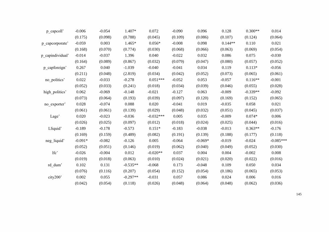
145
p_capcoll’ -0.006 -0.054 1.407* 0.072 -0.090 0.096 0.128 0.300** 0.014
(0.175) (0.098) (0.788) (0.045) (0.109) (0.086) (0.107) (0.124) (0.064)
p_capcorporate’ -0.059 0.003 1.465* 0.056* -0.008 0.098 0.144** 0.110 0.021
(0.168) (0.070) (0.774) (0.030) (0.068) (0.066) (0.063) (0.069) (0.054)
p_capindividual’ -0.014 -0.037 1.396 0.040 -0.022 0.032 0.086 0.075 -0.030
(0.164) (0.089) (0.867) (0.032) (0.079) (0.047) (0.080) (0.057) (0.052)
p_capforeign’ 0.267 0.040 -1.039 -0.040 -0.041 0.034 0.119 0.113* -0.056
(0.211) (0.048) (2.819) (0.034) (0.042) (0.052) (0.073) (0.065) (0.061)
no_politics’ 0.022 -0.033 -0.278 0.051*** -0.052 0.053 -0.057 0.116** -0.001
(0.052) (0.033) (0.241) (0.018) (0.034) (0.039) (0.046) (0.055) (0.028)
high_politics’ 0.062 -0.069 -0.148 -0.021 -0.127 0.063 -0.009 -0.339** -0.092
(0.073) (0.064) (0.193) (0.039) (0.097) (0.120) (0.169) (0.152) (0.065)
no_exporter’ 0.028 -0.074 0.088 0.020 -0.041 0.019 -0.035 0.058 0.021
(0.061) (0.061) (0.139) (0.029) (0.048) (0.032) (0.051) (0.045) (0.037)
Lage’ 0.020 -0.023 -0.036 -0.032*** 0.005 0.035 -0.009 0.074* 0.006
(0.026) (0.025) (0.097) (0.012) (0.018) (0.024) (0.025) (0.044) (0.016)
Lliquid’ -0.189 -0.178 -0.573 0.151* -0.183 -0.038 -0.013 0.363** -0.176
(0.169) (0.159) (0.489) (0.082) (0.191) (0.139) (0.188) (0.177) (0.118)
neg_liquid’ -0.091* -0.082 -0.126 0.005 -0.064 -0.069* -0.019 -0.024 -0.085***
(0.052) (0.051) (0.146) (0.019) (0.062) (0.040) (0.049) (0.052) (0.030)
lfc’ -0.026 -0.004 0.012 -0.020** 0.037 0.004 0.004 -0.002 0.008
(0.019) (0.018) (0.063) (0.010) (0.024) (0.021) (0.020) (0.022) (0.016)
rd_dum’ 0.102 0.131 -0.535** -0.068 0.173 -0.048 0.109 0.050 0.034
(0.076) (0.116) (0.207) (0.054) (0.152) (0.054) (0.186) (0.065) (0.053)
city200’ 0.002 0.055 -0.297** -0.031 0.057 0.086 0.024 0.006 0.016
(0.042) (0.054) (0.118) (0.026) (0.048) (0.064) (0.048) (0.062) (0.036)
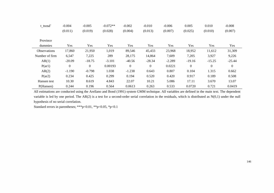
146
t_trend’ -0.004 -0.005 -0.072** -0.002 -0.010 -0.006 0.005 0.010 -0.008
(0.011) (0.019) (0.028) (0.004) (0.013) (0.007) (0.025) (0.010) (0.007)
Province
dummies Yes Yes Yes Yes Yes Yes Yes
Yes
Yes
Observations 17,860 21,950 1,019 89,546 45,433 23,968 18,952 11,612 31,309
Number of firm 6,547 7,225 289 28,175 14,864 7,609 7,205 3,927 9,226
AR(1) -20.09 -18.75 -3.101 -40.56 -28.34 -2.289 -19.16 -15.25 -25.44
P(ar1) 0 0 0.00193 0 0 0.0221 0 0 0
AR(2) -1.190 -0.798 1.038 -1.238 0.643 0.807 0.104 1.315 0.662
P(ar2) 0.234 0.425 0.299 0.194 0.520 0.420 0.917 0.189 0.508
Hansen test 10.30 8.619 4.843 22.07 10.21 5.086 17.11 3.670 13.07
P(Hansen) 0.244 0.196 0.564 0.0613 0.263 0.533 0.0720 0.721 0.0419
All estimations are conducted using the Arellano and Bond (1991) system GMM technique. All variables are defined in the main text. The dependent
variable is led by one period. The AR(2) is a test for a second-order serial correlation in the residuals, which is distributed as N(0,1) under the null
hypothesis of no serial correlation.
Standard errors in parentheses; ***p<0.01, **p<0.05, *p<0.1

147
Table 4.4b: System GMM estimation of the asymmetric threshold model, China 2000-2009 (ii)
Dependent
Variable: Printing Culture
Petroleum
Processing Chemical Medical Rubber Plastic
Non-metal
Products
Metal
Products
lr_stocks sic23 sic24 sic25 sic26 sic27 sic29 sic30 sic31 sic34
Panel A: Short-run dynamics
Speed of
Adjustment
0.388*** 0.501*** 0.490*** 0.552*** 0.312*** 0.408*** 0.337*** 0.121 0.343**
(0.034) (0.086) (0.058) (0.029) (0.063) (0.038) (0.030) (0.083) (0.140)
Panel B: Long-run equilibrium
lr_sales 0.035 0.474*** 0.850*** 0.565*** 0.539*** 0.714*** 0.420*** 0.134 1.693***
(0.444) (0.105) (0.202) (0.147) (0.155) (0.124) (0.087) (0.601) (0.562)
p_capstate -1.844** -0.201 0.123 -0.446*** -0.406*** -0.340 -0.325** -0.304 0.010
(0.724) (0.240) (0.403) (0.098) (0.154) (0.210) (0.148) (0.472) (0.252)
p_capcoll -1.177*** -0.750*** -0.237 -0.845*** -0.405*** -0.649*** -0.772*** -0.332 -0.215
(0.388) (0.183) (0.483) (0.105) (0.144) (0.179) (0.118) (0.411) (0.360)
p_capcorporate -1.158*** -0.551*** -0.065 -0.611*** -0.265** -0.636*** -0.562*** -0.192 -0.437***
(0.347) (0.114) (0.413) (0.058) (0.116) (0.147) (0.089) (0.353) (0.167)
p_capindividual -1.240*** -0.630*** 0.175 -0.727*** -0.298** -0.574*** -0.684*** -0.245 -0.307
(0.376) (0.111) (0.432) (0.080) (0.120) (0.148) (0.085) (0.368) (0.268)
p_capforeign -0.001 -0.063 0.597 -0.006 0.130 0.072 0.045 0.358 -0.239
(0.188) (0.093) (0.510) (0.070) (0.138) (0.138) (0.077) (0.400) (0.163)
no_politics 0.042 -0.124 -0.087 -0.151*** -0.032 -0.087 -0.107** 0.031 0.073
(0.078) (0.079) (0.096) (0.041) (0.060) (0.078) (0.052) (0.171) (0.124)
high_politics 0.769** -0.111 0.211 0.256** 0.083 0.143 0.318*** 0.976 -0.245
(0.358) (0.190) (0.431) (0.101) (0.088) (0.154) (0.113) (0.630) (0.376)
no_exporter -0.759*** -0.216*** -0.334 -0.519*** -0.306*** -0.431*** -0.431*** -0.612** 0.169

148
(0.236) (0.075) (0.285) (0.106) (0.114) (0.089) (0.061) (0.307) (0.301)
lage 0.116** 0.157** 0.063 0.139*** 0.149*** 0.193*** -0.050 -0.155 0.114**
(0.056) (0.068) (0.060) (0.025) (0.056) (0.054) (0.045) (0.197) (0.053)
lliquid -1.279** -0.525** -0.298 -0.610*** 0.094 -0.131 -0.646*** 0.997 0.109
(0.517) (0.242) (0.459) (0.181) (0.278) (0.307) (0.216) (1.066) (0.589)
neg_liquid -0.253* -0.165** -0.039 -0.093*** -0.031 -0.013 -0.261*** -0.076 0.021
(0.132) (0.069) (0.106) (0.031) (0.082) (0.088) (0.064) (0.227) (0.080)
lfc 0.178*** 0.231*** 0.221*** 0.149*** 0.177*** 0.233*** 0.254*** 0.280** 0.368**
(0.041) (0.053) (0.065) (0.028) (0.025) (0.047) (0.034) (0.119) (0.176)
rd_dum 1.161** 0.298*** 0.172 0.500*** 0.397*** 0.362*** 0.459*** 0.888 -0.523
(0.520) (0.095) (0.282) (0.120) (0.087) (0.097) (0.088) (0.607) (0.573)
city200 0.316 0.038 -0.099 0.048 -0.079 0.051 -0.222** 0.062 0.088
(0.228) (0.108) (0.103) (0.037) (0.081) (0.134) (0.089) (0.160) (0.109)
t_trend 0.108 -0.000 -0.107*** -0.044*** -0.025 -0.106*** -0.018 -0.011 -0.225**
(0.077) (0.015) (0.032) (0.017) (0.022) (0.019) (0.012) (0.107) (0.109)
Effects of the business cycle dummy variable:
Panel C: Short-run dynamics
Speed of
Adjustment’
0.005*** 0.015*** -0.006*** 0.010*** 0.007*** 0.002*** 0.002*** 0.013*** 0.020***
(0.005) (0.004) (0.012) (0.005) (0.005) (0.006) (0.003) (0.009) (0.016)
Panel D: Long-run equilibrium
lr_sales’ 0.367 -0.065** -0.136 0.509* -0.027 -0.084** 0.066* 0.155 -0.618*
(0.258) (0.032) (0.192) (0.283) (0.073) (0.042) (0.038) (0.120) (0.347)
p_capstate’ 0.599 -0.130 -0.173 0.322* 0.090 -0.189* 0.050 0.062 -0.249
(0.468) (0.152) (0.238) (0.170) (0.074) (0.103) (0.071) (0.103) (0.165)
p_capcoll’ 0.267 0.002 -0.119 0.320** 0.057 -0.032 0.125** 0.018 -0.365
(0.239) (0.095) (0.351) (0.162) (0.061) (0.093) (0.050) (0.070) (0.224)
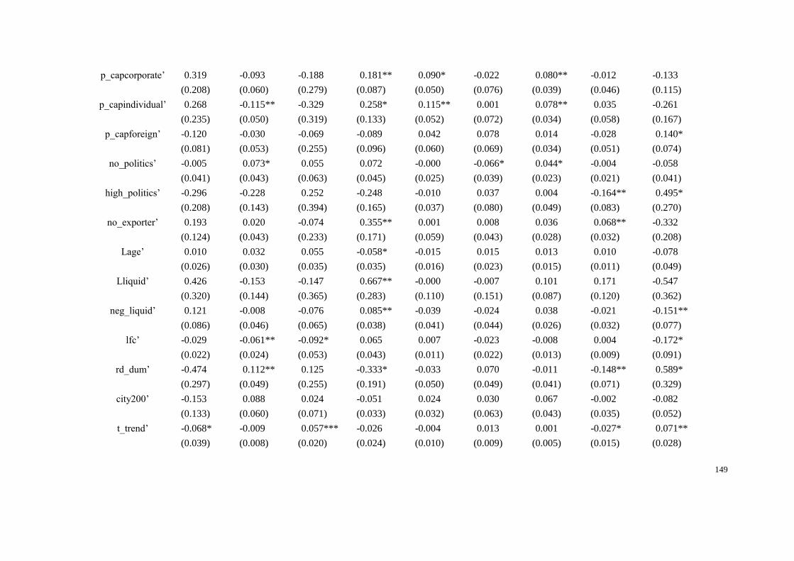
149
p_capcorporate’ 0.319 -0.093 -0.188 0.181** 0.090* -0.022 0.080** -0.012 -0.133
(0.208) (0.060) (0.279) (0.087) (0.050) (0.076) (0.039) (0.046) (0.115)
p_capindividual’ 0.268 -0.115** -0.329 0.258* 0.115** 0.001 0.078** 0.035 -0.261
(0.235) (0.050) (0.319) (0.133) (0.052) (0.072) (0.034) (0.058) (0.167)
p_capforeign’ -0.120 -0.030 -0.069 -0.089 0.042 0.078 0.014 -0.028 0.140*
(0.081) (0.053) (0.255) (0.096) (0.060) (0.069) (0.034) (0.051) (0.074)
no_politics’ -0.005 0.073* 0.055 0.072 -0.000 -0.066* 0.044* -0.004 -0.058
(0.041) (0.043) (0.063) (0.045) (0.025) (0.039) (0.023) (0.021) (0.041)
high_politics’ -0.296 -0.228 0.252 -0.248 -0.010 0.037 0.004 -0.164** 0.495*
(0.208) (0.143) (0.394) (0.165) (0.037) (0.080) (0.049) (0.083) (0.270)
no_exporter’ 0.193 0.020 -0.074 0.355** 0.001 0.008 0.036 0.068** -0.332
(0.124) (0.043) (0.233) (0.171) (0.059) (0.043) (0.028) (0.032) (0.208)
Lage’ 0.010 0.032 0.055 -0.058* -0.015 0.015 0.013 0.010 -0.078
(0.026) (0.030) (0.035) (0.035) (0.016) (0.023) (0.015) (0.011) (0.049)
Lliquid’ 0.426 -0.153 -0.147 0.667** -0.000 -0.007 0.101 0.171 -0.547
(0.320) (0.144) (0.365) (0.283) (0.110) (0.151) (0.087) (0.120) (0.362)
neg_liquid’ 0.121 -0.008 -0.076 0.085** -0.039 -0.024 0.038 -0.021 -0.151**
(0.086) (0.046) (0.065) (0.038) (0.041) (0.044) (0.026) (0.032) (0.077)
lfc’ -0.029 -0.061** -0.092* 0.065 0.007 -0.023 -0.008 0.004 -0.172*
(0.022) (0.024) (0.053) (0.043) (0.011) (0.022) (0.013) (0.009) (0.091)
rd_dum’ -0.474 0.112** 0.125 -0.333* -0.033 0.070 -0.011 -0.148** 0.589*
(0.297) (0.049) (0.255) (0.191) (0.050) (0.049) (0.041) (0.071) (0.329)
city200’ -0.153 0.088 0.024 -0.051 0.024 0.030 0.067 -0.002 -0.082
(0.133) (0.060) (0.071) (0.033) (0.032) (0.063) (0.043) (0.035) (0.052)
t_trend’ -0.068* -0.009 0.057*** -0.026 -0.004 0.013 0.001 -0.027* 0.071**
(0.039) (0.008) (0.020) (0.024) (0.010) (0.009) (0.005) (0.015) (0.028)

150
Province
dummies Yes Yes Yes Yes Yes Yes Yes
Yes
Yes
Observations 19,503 12,393 6,936 80,370 21,714 11,537 39,503 90,496 54,683
Number of firm 5,903 3,867 2,349 24,741 6,060 3,690 13,447 27,603 20,859
AR(1) -16.90 -3.125 -11.37 -36.64 -20.38 -15.21 -27.03 -2.766 -8.897
P(ar1) 0 0.00178 0 0 0 0 0 0.00568 0
AR(2) -1.625 -0.855 1.623 -1.439 -1.843 -1.303 -2.038 0.848 -1.535
P(ar2) 0.104 0.392 0.105 0.150 0.0747 0.193 0.0415 0.396 0.125
Hansen test 8.956 13.57 9.470 3.250 9.276 6.846 12.89 7.500 0.307
P(Hansen) 0.346 0.194 0.0504 0.517 0.0667 0.144 0.0426 0.277 0.857
All estimations are conducted using the Arellano and Bond (1991) system GMM technique. All variables are defined in the main text. The dependent
variable is led by one period. The AR(2) is a test for a second-order serial correlation in the residuals, which is distributed as N(0,1) under the null
hypothesis of no serial correlation.
Standard errors in parentheses; ***p<0.01, **p<0.05, *p<0.1

151
Table 4.4c: System GMM estimation of the asymmetric threshold model, China 2000-2009 (iii)
Dependent
Variable:
Machinery &
Equipment
Transport
Equipment
Measuring
Instrument
Other
Manufacturing
Electronic
Power
Gas
Production
Water
Production
Coal
Mining
lr_stocks sic35 sic37 sic41 sic43 sic44 sic45 sic46 sic60
Panel A: Short-run dynamics
Speed of
Adjustment
0.264*** 0.518*** 0.428*** 0.404*** 0.516*** 0.488*** 0.423*** 0.592***
(0.017) (0.108) (0.033) (0.026) (0.049) (0.087) (0.042) (0.038)
Panel B: Long-run equilibrium
lr_sales 0.733*** 0.950*** 0.874*** 0.574*** 0.974*** 1.077*** 0.841*** 0.651***
(0.085) (0.185) (0.093) (0.063) (0.223) (0.358) (0.171) (0.149)
p_capstate -0.043 -0.050 0.069 -0.309** -0.960* 0.654 1.261** 0.004
(0.110) (0.157) (0.139) (0.133) (0.529) (0.405) (0.568) (0.747)
p_capcoll -0.581*** -0.458*** -0.329** -0.545*** -0.860 0.044 1.263** -0.596
(0.095) (0.087) (0.154) (0.139) (0.577) (0.613) (0.570) (0.749)
p_capcorporate -0.513*** -0.415*** -0.269*** -0.583*** -0.822** 0.712* 1.288** -0.497
(0.073) (0.071) (0.094) (0.090) (0.402) (0.386) (0.546) (0.725)
p_capindividual -0.524*** -0.548*** -0.457*** -0.611*** -0.771 0.892 0.662 -0.450
(0.075) (0.073) (0.096) (0.085) (0.529) (0.588) (0.555) (0.731)
p_capforeign 0.076 -0.024 -0.130 0.024 -0.221 0.101 0.217 1.448*
(0.075) (0.149) (0.100) (0.093) (0.291) (0.404) (0.980) (0.841)
no_politics -0.085** -0.108*** -0.021 0.020 0.076 -0.168 0.174 0.084
(0.037) (0.033) (0.058) (0.058) (0.090) (0.226) (0.192) (0.071)
high_politics 0.373*** 0.229** 0.060 0.588*** -0.122 -0.269 -0.638 0.938***
(0.062) (0.117) (0.104) (0.117) (0.320) (0.521) (0.388) (0.274)
no_exporter -0.255*** -0.163 -0.093 -0.119** -0.415 -0.327 0.685 0.150
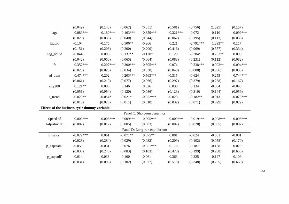
152
(0.049) (0.140) (0.067) (0.051) (0.581) (0.756) (1.025) (0.157)
lage 0.089*** 0.180*** 0.163*** 0.359*** -0.321*** -0.072 -0.110 0.099***
(0.028) (0.033) (0.040) (0.044) (0.062) (0.195) (0.113) (0.036)
lliquid -0.104 -0.175 -0.506** -0.266 0.221 -2.791*** 1.393** 0.117
(0.151) (0.203) (0.200) (0.200) (0.416) (0.969) (0.557) (0.334)
neg_liquid -0.044 0.006 -0.137** -0.120* 0.120 -0.384* 0.232** 0.000
(0.042) (0.050) (0.065) (0.064) (0.083) (0.231) (0.112) (0.082)
lfc 0.352*** 0.207*** 0.300*** 0.305*** 0.074 0.238*** 0.092** 0.094***
(0.023) (0.028) (0.034) (0.038) (0.048) (0.088) (0.036) (0.033)
rd_dum 0.474*** 0.202 0.203*** 0.563*** -0.315 -0.624 0.255 0.744***
(0.061) (0.219) (0.077) (0.066) (0.297) (0.379) (0.288) (0.167)
city200 0.121** 0.005 0.146 0.026 0.038 0.134 -0.084 -0.048
(0.051) (0.054) (0.120) (0.086) (0.123) (0.310) (0.144) (0.059)
t_trend -0.029** -0.054* -0.021* -0.052*** -0.029 -0.182** -0.013 -0.073***
(0.013) (0.028) (0.011) (0.010) (0.032) (0.071) (0.029) (0.022)
Effects of the business cycle dummy variable:
Panel C: Short-run dynamics
Speed of
Adjustment’
0.003*** -0.005*** 0.009*** 0.005*** -0.009*** 0.019*** 0.008*** 0.005***
(0.002) (0.012) (0.005) (0.003) (0.007) (0.020) (0.005) (0.007)
Panel D: Long-run equilibrium
lr_sales’ -0.072*** 0.061 -0.071** 0.075** 0.081 -0.024 -0.061 -0.081
(0.028) (0.284) (0.029) (0.032) (0.209) (0.102) (0.058) (0.170)
p_capstate’ -0.059 -0.031 0.076 -0.351*** 0.176 -0.187 -0.138 0.020
(0.038) (0.240) (0.083) (0.103) (0.473) (0.199) (0.258) (0.658)
p_capcoll’ -0.014 -0.038 0.100 -0.061 0.363 0.225 -0.197 0.109
(0.031) (0.093) (0.102) (0.077) (0.519) (0.348) (0.265) (0.669)
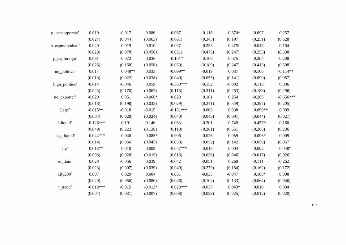
153
p_capcorporate’ 0.019 -0.017 0.086 -0.087 0.116 -0.374* -0.097 0.257
(0.024) (0.044) (0.063) (0.061) (0.343) (0.197) (0.251) (0.628)
p_capindividual’ -0.020 -0.019 0.010 -0.037 0.233 -0.475* -0.013 0.104
(0.023) (0.078) (0.056) (0.051) (0.475) (0.247) (0.253) (0.638)
p_capforeign’ 0.031 -0.072 0.036 -0.101* 0.108 0.075 0.204 -0.208
(0.026) (0.168) (0.056) (0.059) (0.189) (0.247) (0.413) (0.598)
no_politics’ 0.014 0.048** 0.033 -0.099** -0.019 0.037 -0.106 -0.114**
(0.013) (0.022) (0.038) (0.040) (0.055) (0.141) (0.090) (0.057)
high_politics’ -0.014 -0.046 0.059 -0.360*** -0.152 -0.082 0.116 0.036
(0.023) (0.170) (0.062) (0.113) (0.311) (0.253) (0.188) (0.296)
no_exporter’ -0.020 0.051 -0.066* 0.023 0.181 0.254 -0.286 -0.656***
(0.018) (0.198) (0.035) (0.029) (0.341) (0.349) (0.394) (0.205)
Lage’ -0.015** -0.018 -0.015 -0.131*** 0.006 0.038 0.090** 0.009
(0.007) (0.028) (0.024) (0.040) (0.043) (0.091) (0.044) (0.027)
Lliquid’ -0.126*** -0.191 -0.146 -0.063 -0.201 0.749 -0.457* 0.160
(0.049) (0.222) (0.128) (0.110) (0.261) (0.551) (0.268) (0.236)
neg_liquid’ -0.044*** -0.040 -0.085* -0.006 0.026 0.059 -0.096* 0.009
(0.014) (0.056) (0.045) (0.038) (0.052) (0.142) (0.056) (0.067)
lfc’ -0.013** -0.010 -0.009 -0.047*** -0.018 -0.004 -0.002 0.048*
(0.006) (0.028) (0.019) (0.016) (0.036) (0.046) (0.017) (0.026)
rd_dum’ 0.020 -0.056 0.039 -0.042 -0.051 0.260 -0.111 -0.262
(0.023) (0.307) (0.039) (0.040) (0.279) (0.184) (0.162) (0.172)
city200’ 0.007 0.029 0.004 0.031 -0.035 -0.047 0.108* 0.008
(0.020) (0.056) (0.080) (0.046) (0.102) (0.133) (0.064) (0.046)
t_trend’ -0.013*** -0.015 -0.012* 0.023*** -0.027 0.043* 0.010 0.004
(0.004) (0.031) (0.007) (0.008) (0.028) (0.025) (0.012) (0.020)

154
Province dummies Yes Yes Yes Yes Yes Yes Yes
Yes
Observations 148,039 44,393 14,754 25,924 15,860 1,864 9,062 16,248
Number of firm 49,026 13,999 6,556 9,354 4,473 535 2,293 5,521
AR(1) -49.39 -18.75 -12.63 -20.88 -15.55 -6.539 -15.29 -19.54
P(ar1) 0 0 0 0 0 6.17e-11 0 0
AR(2) -2.032 1.015 -0.0689 -1.735 -1.366 -1.391 -0.890 -1.637
P(ar2) 0.0496 0.310 0.945 0.0827 0.172 0.164 0.373 0.102
Hansen test 19.84 1.917 5.006 4.735 9.387 2.488 2.022 9.637
P(Hansen) 0.0208 0.384 0.287 0.786 0.153 0.647 0.732 0.131
All estimations are conducted using the Arellano and Bond (1991) system GMM technique. All variables are defined in the main text. The
dependent variable is led by one period. The AR(2) is a test for a second-order serial correlation in the residuals, which is distributed as N(0,1)
under the null hypothesis of no serial correlation.
Standard errors in parentheses; ***p<0.01, **p<0.05, *p<0.1
155
4.4 Conclusions
In this chapter, we employed the asymmetric error-correction model in order to detect
the asymmetric adjustment mechanism. The whole sample is divided into two parts
according to the industry-specific business cycle, and the deviations of the estimated
coefficients between the upswing and downswing parts provide evidence on the
mechanism of asymmetric adjustment.
Generally speaking, the asymmetric mechanism in the adjustment model could be
commonly found in the short-run: during bad business environment, firms become
more sensitive and react quicker when they confront the demand shocks. However, the
target inventory level indicators seem to performance symmetrically regardless of the
exogenous business movements. Reminded that fluctuations with periods between 1.5
and 8 years are considered to be business-cycle fluctuations, Chinese manufacturers
could adjust their inventory accumulation speed efficiently when business
environment change. But the arrangement of their target inventory level according to
specific characteristics is not flexible, and it will cost a long time so that firms could
shift their target inventory to another level during the business cycle fluctuation. One
possible explanation could be that the development of inventory management is not as
much as expectation and the implementation of recent management developments,

156
such as JIT, WCM and advanced IT, needs to be considered critically in the Chinese
context.

157
Chapter 5. The role of innovation in
inventory performance: a total factor
productivity perspective

158
Chapter 5. The role of innovation in inventory
performance: a total factor productivity perspective
5.1 Introduction
“Inventory management” and “investment in innovations” has generated great interest
in the academic and business press in recent years. It is said that inventory reduction
has been a remarkable outcome of inventory management, and a flourishing literature
states that the inventory reduction diminishes working capital investment needs and
releases funds for alternative uses. In order to maintain competitive advantage, firms
have been investing heavily in intangible resources, especially innovations, over the
past decade (Zhou et al., 2011). For example, Science and Engineering Indicators:
2010 (National Science Board, 2010) reports that the global research and development
(R&D) expenditure has doubled from $525 billion in 1996 to $1.1 trillion in 2007. The
U.S. leads all other countries in R&D expenditure, with $369 billion in 2007.
However, prior studies show no clear consensus on the relationship between
innovations and inventory performance (Cannon, 2008). The success in
implementation of inventory management innovations is not universal since the
adoption of initiatives such as JIT and WCM requires significant organisational effort

159
and change. Besides, the inventory reduction puts pressure on internal operations to
improve (e.g. quality, logistics, production flexibility and operational efficiency) by
taking away the convenient supply and/or demand buffer. This chapter attempts to
associates a firm’s inventory performance with its capabilities of utilizing the
technology progress and technical efficiency improvement, approximated here by total
factor productivity.
Remained that in Chapter 3 and Chapter 4, the R&D dummy, firm age, time trend and
a location dummy are included in our dynamic inventory adjustment model to capture
innovations. However, these factors are only indirect indicators, and we could not find
clear evidence to support the link between technical improvement and inventory
reduction using these measurements. For instance, R&D is expected to have a positive
impact on inventory level reduction however the estimated coefficient of R&D dummy
is significantly positive for a majority of industries, which is opposite to the prediction.
This could be due to the fact that firms in developing countries are too far from the
technological frontier, and R&D investment could require longer time horizons to
demonstrate results (Crespi and Zuniga, 2012). Moreover, firms that have the ability
to spend on R&D could be seen as financially unconstrained and, therefore, are willing
to have a higher level of inventories (Ughetto, 2008).

160
TFP, which attempts to measure the change in output net of the change in all inputs, is
a more comprehensive indicator when we examine the impact of innovation on
inventory performance in the Chinese market. TFP is commonly regarded as a measure
of productivity (Lieberman and Asaba, 1997) and findings of the empirical studies
show that one of the important sources of the productivity heterogeneity at the firm
level is related to R&D and innovation activities (Griliches, 1998). More often than
not, the concept of TFP change is used synonymously with technological progress and
technical efficiency change in the productivity literature (Nishimizu and Page, 1982).
The technological progress is defined as the movement of the best practice or frontier
production function over time, and the technical efficiency change refers to all other
factors affecting productivity that move the firm towards the current best practice
frontier.
Decomposition of TFP into technological progress and technical efficiency
improvement is vital when analysing the impact of innovation on inventory
performance, especially in developing countries (Felipe, 1999). In the previous
chapters, the failure of the R&D dummy in capturing the development of inventory
management is due to the fact that, in an economy such as China which “borrows”
technology extensively from abroad, failures to acquire and adapt technology to new
international standards will be reflected in the lack of technological progress at the

161
frontier. Moreover, Cassiman et al. (2010) suggests that different innovation activities
tend to affect productivity differentially: Product innovation should relate more to
firm-specific demand variations whereas process innovation is expected to affect
technical efficiency; and thus the use of R&D can be seen as an imperfect proxy
because it can be related, differently, to both types of innovation.
Comin and Mulani (2009) model the development of disembodied innovations such as
managerial and organizational techniques, personnel, accounting, work practices and
financial innovations, and claim the contributions of this kind of innovations to TFP.
According to Yue and Liu (2006), in China, TFP growth is found for the data period
1996-2003, and it is accomplished mainly through the efficiency improvement which
was underestimated by previous studies. Several improvements in inventory and SCM
are more likely to be classified as technical efficiency changes and therefore, the TFP
seems to be a more complex indicator.
Accordingly, in this chapter, we re-estimate the error-correction model augmented
with a proxy for TFP to further analyse the inventory reduction effect of productivity
improvement which is mainly related to process and efficiency innovations. Our
research makes two significant contributions to the inventory management literature.
First, to the best of our knowledge, we are the first to empirically link TFP to inventory
performance. By taking innovations, especially process and efficiency
162
improvements into consideration, we find that the effectiveness with which a firm
utilizes its factor inputs affects its inventory level significantly. Second, we empirically
examine the inventory reducing impact of process innovation under different business
environment. By doing this, it could be proved that the benefits of productivity
improvement and technical efficiency innovations cannot be discharged by demand
shocks.
This chapter is organized as follows: Section 2 is a review of inventory reducing
impact of TFP; Section 3 is the theoretical and empirical background on conducting
TFP; Section 4 introduces the data involved and provides the descriptive statistics;
Section 5 includes the research methods for symmetric and asymmetric inventory
adjustment model followed by the results discussion. The conclusion of this chapter
will be presented in Section 6.
5.2 Review of inventory reducing impact of total factor
productivity
Since TFP in this chapter is used to proxy how successful a firm is at adopting new
technological progress and technical efficiency improvement, the relationships

163
between inventory performance and two different types of innovation (product
innovation and process innovation) are discussed, and the impacts of TFP on inventory
are summarized in Table 5.1.
Table 5.1: Summary of inventory reducing impact of TFP
Innovation Method Impact
Product innovation
(Technological progress)
Supply of a new product Inventory volume (-)
Effect of learning curves Inventory volume (-)
Management of product transition Inventory volume (-)
Process innovation
(Technical efficiency)
Flow time Inventory volume (-)
Waste, defects and returns Inventory volume (-)
Recorder point and safety inventory Inventory volume (-)
5.2.1 Product innovation
Product innovation may affect inventory level in three ways: the supply of a new
product, the effect of learning curves, and the management of product transition (Zhou
et al., 2011).
Supply of a new product
For a new-product introduction, firms can choose either the expand-early or the wait-
and-see strategy to determine the timing of production expansion (Stevenson, 2009).
The expand-early strategy increases the amount of production before the demand
increment and results in an inventory surplus. Firms choose this strategy if the cost of

164
lost sales is high, the demand increment is fairly certain, the economy of scale
generates great savings, or if their priority is competing for market shares. Firms
adopting the wait-and-see strategy tend to increase actual production after the demand
increment is realized. Firms prefer this strategy if adding capacity is expensive or if
the technology becomes obsolete quickly. This strategy implies relatively high
inventory turnover; firms can maintain a low inventory level and might even
experience a shortage and backlog in inventory. Because of the uncertain nature of
new-product introduction, it is very likely that firms that are afraid of committing
themselves to a large production level will adopt the wait-and-see strategy keeping
inventory volume relatively low in the product life cycle.
Effect of learning curves
Norton and Bass (1987) extend the original Bass diffusion model to incorporate
successive generations of technology. According to the Norton-Bass model, if a firm
invents new products on a regular basis, the same diffusion process is valid for each
generation. After repeatedly facing challenges in production planning and inventory
management in the product innovation process, a firm might learn from its past
experiences/mistakes and become more sophisticated in managing inventory. For
example, a firm might achieve a more accurate demand forecast for its new products.

165
We, therefore, could suggest that product innovation enhances a firm’s ability to
manage its inventory level through learning by doing.
Management of product transition
It is important that firms with frequent new product introductions properly manage
inventory during product transitions. In the early introduction stage, immature
manufacturing processes and technologies can cause high defective rates, forcing firms
to carry more inventory as a buffer against production disruptions. Another factor that
can lead to higher inventory levels for new products is the potential for return and
exchange requests due to defects. In addition, the new product can speed up the
obsolescence of old products; if the transition is not properly managed, the firm can
end up with an excessive inventory of old products. Therefore, it seems to be that firms
with frequent product innovation will become increasingly efficient in inventory
management as they gain experience in handling product transitions.
5.2.2 Process innovation
A process innovation could reduce production cost, increase production efficiency,
and/or improve product quality and contribute to flexible product lines, low waste, and
on-time delivery.
166
Flow time
Flow time, the time required to transform raw materials into finished products, has
been a key indicator of the efficiency of a production system since the late 19th century.
According to Little’s law (Little, 1961), if a firm shortens flow time, either by
modifying the process or by enhancing productivity, the inventories of raw materials,
work-in-progress, and finished products will be reduced, and inventory turnover will
improve.
Waste, defects and returns
An advanced production system tends to reduce mistakes and defects on the production
line, save waste resulting from discarded defective parts or products and increase the
consistency of product quality. For example, Lieberman and Demeester (1999) claim
that JIT has been successful in eliminating defects. By lowering defect rates, a firm
can reduce the amount of buffer inventory required to guard against production
disruptions. Besides, consistent product quality means fewer returns or exchanges
from customers, and this could be a further reason for firms to lower inventory.
Reorder point and safety inventory
As discussed earlier, a major benefit of process innovation is the reduced flow time
and hence the reduced production lead time. A shorter and more consistent lead time
167
means a lower reorder point, the inventory level at which a firm places its production
orders, in a continuous review system (Stevenson, 2009). It also means that there
would be no need to carry a high safety inventory as a buffer against potential stockout
risks. Reducing reorder point and safety inventory will improve inventory turnover
and keep the inventory level under a relatively low level.
5.3 Total factor productivity in Chinese manufacturing
industries
Studies focusing on TFP in China are quite limited. Recent research conducted by Guo
and Jia (2005) provide a general description about TFP. It is claimed that the TFP
growth rate experienced severe fluctuations from 1979-1993. The growth rate
decreased from 1993 to 2000, after which the growth rate increases steadily. These
fluctuations may be due to the economic structure transition. During the research
period, it is found that the TFP growth rate in China is higher than that in developed
countries (Japan, Germany and the US) but lower than developing countries such as
Thailand, Singapore and South Korea. Ding et al. (2014) estimate TFP growth in China
for 1998 to 2007, and it is said that the growth rate is very high during that period of
time.

168
The objective of productivity measurement is to identify output differences that cannot
be explained by input differences (Van Biesebroeck, 2007). The paper conducted by
Ding et al. (2014) is one of a small number of papers that examine firm-level TFP and
its determinants in China. A Cobb-Douglas log-linear production function approach
including fixed effects is employed in order to calculate TFP:
𝑦𝑖𝑡 = 𝛼𝑖 + 𝛼𝐸𝑒𝑖𝑡 + 𝛼𝑀𝑚𝑖𝑡 + 𝛼𝐾𝑘𝑖𝑡 + 𝛼𝑋𝑋𝑖𝑡 + 𝛼𝑇𝑡 + 휀𝑖𝑡 (5.1)
where endogenous y, e, m and k refer respectively to the logarithms of real gross
output, employment, intermediate inputs, and the capital accumulation in firm i at time
t; and Xit is a vector of observed (proxy) variables determining TFP. More specifically,
they include firm characteristics such as firm age, political affiliation, firm ownership,
export behaviour, whether the firm engaged in R&D, financial variables, and
geographic location into the vector Xit. Lastly, t is a time trend, measuring exogenous
gains in TFP over time.
Ding et al. (2014) first estimates equation (5.1) for different industries and obtain an
unbiased estimation of elasticity of output with respect to inputs ( E , M and K ).
TFP can then be calculated as the level of output that is not attributable to factor inputs
(employment, intermediate inputs and capital). In other words, productivity is due to

169
efficiency levels and technical progress. Thus, such a measure of TFP can be expressed
as:
𝑙𝑛𝑇𝐹�̂�𝑖𝑡 = 𝑦𝑖𝑡 − 𝑎�̂�𝑒𝑖𝑡 − 𝑎�̂�𝑚𝑖𝑡 − 𝑎�̂�𝑘𝑖𝑡 = 𝑎�̂� + 𝑎�̂�𝑋𝑖𝑡 + 𝑎�̂�𝑡 + 휀𝑖𝑡 (5.2)

170
Table 5.2a: Long-run two-step system-GMM production function, various industries, China 2000-2007 (i)
Dependent
Variable:
Other
Mining
Food
Production Tobacco Textile
Apparel &
Footwear Leather Timber
Furniture
Paper-making
ln_sales sic10+80 sic14 sic16 sic17 sic18 sic19 sic20 sic21 sic22
ln intermediate
inputs 0.308*** 0.366*** 0.386*** 0.853*** 0.653*** 0.763*** 0.493*** 0.494*** 0.843***
(0.074) (0.157) (0.082) (0.019) (0.049) (0.058) (0.118) (0.068) (0.032)
ln employment 0.505*** 0.311* 0.613** 0.153*** 0.294*** 0.095*** 0.483*** 0.446*** 0.166***
(0.064) (0.174) (0.287) (0.033) (0.041) (0.053) (0.114) (0.078) (0.045)
ln capital 0.225*** 0.357* 0.387** 0.037** 0.085*** 0.143*** 0.130* 0.169*** 0.040***
(0.065) (0.196) (0.161) (0.019) (0.038) (0.073) (0.076) (0.046) (0.009)
Standard errors in parentheses; ***p<0.01, **p<0.05, *p<0.1
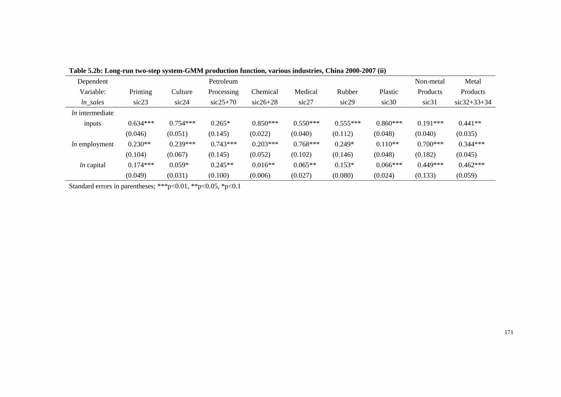
171
Table 5.2b: Long-run two-step system-GMM production function, various industries, China 2000-2007 (ii)
Dependent
Variable: Printing Culture
Petroleum
Processing Chemical Medical Rubber Plastic
Non-metal
Products
Metal
Products
ln_sales sic23 sic24 sic25+70 sic26+28 sic27 sic29 sic30 sic31 sic32+33+34
ln intermediate
inputs 0.634*** 0.754*** 0.265* 0.850*** 0.550*** 0.555*** 0.860*** 0.191*** 0.441**
(0.046) (0.051) (0.145) (0.022) (0.040) (0.112) (0.048) (0.040) (0.035)
ln employment 0.230** 0.239*** 0.743*** 0.203*** 0.768*** 0.249* 0.110** 0.700*** 0.344***
(0.104) (0.067) (0.145) (0.052) (0.102) (0.146) (0.048) (0.182) (0.045)
ln capital 0.174*** 0.059* 0.245** 0.016** 0.065** 0.153* 0.066*** 0.449*** 0.462***
(0.049) (0.031) (0.100) (0.006) (0.027) (0.080) (0.024) (0.133) (0.059)
Standard errors in parentheses; ***p<0.01, **p<0.05, *p<0.1
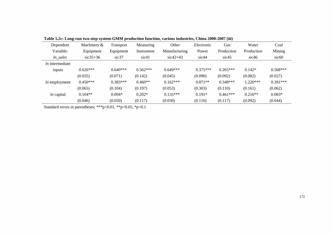
172
Table 5.2c: Long-run two-step system-GMM production function, various industries, China 2000-2007 (iii)
Dependent
Variable:
Machinery &
Equipment
Transport
Equipment
Measuring
Instrument
Other
Manufacturing
Electronic
Power
Gas
Production
Water
Production
Coal
Mining
ln_sales sic35+36 sic37 sic41 sic42+43 sic44 sic45 sic46 sic60
ln intermediate
inputs 0.626*** 0.640*** 0.562*** 0.649*** 0.375*** 0.265*** 0.142* 0.568***
(0.035) (0.071) (0.142) (0.045) (0.090) (0.092) (0.082) (0.027)
ln employment 0.450*** 0.383*** 0.460** 0.162*** 0.871** 0.348*** 1.220*** 0.391***
(0.065) (0.104) (0.197) (0.053) (0.303) (0.110) (0.161) (0.062)
ln capital 0.104** 0.094* 0.202* 0.135*** 0.191* 0.461*** 0.216** 0.083*
(0.046) (0.050) (0.117) (0.030) (0.110) (0.117) (0.092) (0.044)
Standard errors in parentheses; ***p<0.01, **p<0.05, *p<0.1

173
Table 5.2a, Table 5.2b and Table 5.2c present estimated coefficients of inputs ( E ,
M and K ) of the long-run two-step system-GMM production function (equation 5.1)
covering the Chinese manufacturing industries through 1998-2007 (Ding et al., 2014).
Equation 5.1 was estimated, in dynamic form with additional lagged values of output
and factor inputs, using the system GMM approach since it is sufficiently flexible to
allow for both endogenous regressors and a first-order autoregressive error term. The
elasticities of output with respect to intermediate input, labor and capital display
significant heterogeneity among various industries. Since we employ the same dataset
as Ding et al. (2014), these coefficients are used directly to predict firm-level TFP
values, based on equation 5.2.
5.4 Data and descriptive statistics
Due to data availability (data related to intermediate inputs are not recorded in 2008
and 2009), the sample period is 2000-2007 in this chapter. Table 5.3 summarises the
average overall TFP value, adjusted average TFP value (after normalising the value of
TFP in 1998 to 1 for all firms) and the number of observations for each year. The
number of observations ranges from a minimum of 126,444 firms in 2000 to a
maximum of 261,765 firms in 2007. Consistent with Guo and Jia (2005), Figure 5.1
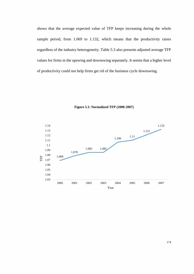
174
shows that the average expected value of TFP keeps increasing during the whole
sample period, from 1.069 to 1.132, which means that the productivity raises
regardless of the industry heterogeneity. Table 5.3 also presents adjusted average TFP
values for firms in the upswing and downswing separately. It seems that a higher level
of productivity could not help firms get rid of the business cycle downswing.
Figure 5.1: Normalized TFP (2000-2007)
1.069
1.078
1.085 1.085
1.1061.11
1.121
1.132
1.03
1.04
1.05
1.06
1.07
1.08
1.09
1.1
1.11
1.12
1.13
1.14
2000 2001 2002 2003 2004 2005 2006 2007
TF
P
Year

175
Table 5.3: Descriptive statistics (2000-2007)
2000 2001 2002 2003 2004 2005 2006 2007 2000-2007 upswing downswing
N 126,444 132,877 143,781 153,547 219,819 214,915 238,160 261,765 1,491,308 739,946 751,153
Mean (Ln TFP) -2.674 -2.553 -2.469 -2.469 -2.243 -2.204 -2.115 -2.023 -2.288 -2.343 -2.233
Normalization
(Ln TFP1998=1) 1.069 1.078 1.085 1.085 1.106 1.110 1.121 1.132 1.101 1.096 1.107
Ste. Dev. 1.836 1.803 1.779 1.699 1.585 1.547 1.498 1.400 1.625 1.636 1.611
176
5.5 Empirical models and results
5.5.1 Symmetric inventory adjustment approach
In addition to Chapter 3, we re-estimate the target adjustment inventory model
augmented with the predicted TFP:
𝐼𝑖𝑡 = 𝜑𝐼𝑖,𝑡−1 + 𝜋′𝑋𝑖𝑡 + 𝑣𝑖𝑡 (5.3)
where the variables are expressed in logarithms and itI refers to the amount of
inventories and Xit denotes the k×1 vector of variables that determining target level
of inventory. In addition to the factors that are estimated in the previous chapters, the
predicted TFP variable is now also included in Xit .
Consistent with the approach used in previous chapters, the two steps system-GMM
estimator is employed and TFP is treated as endogenous and is therefore instrumented
using lagged values of itself as the instruments. We report the main estimation results
for 26 two-digit industries/industry groups in Table 5.4(a), Table 5.4(b) and Table
5.4(c). Panel A presents the short-run dynamics, including the short-run coefficients
of lags 1 and 2 of inventory level while panel B contains the long-run coefficients on
the determinants of target inventory level. We focus on the coefficients on TFP and
177
technology-related variables in this study. The AR(2) and Hansen test of no second-
order autocorrelation and valid instruments cannot be rejected at 5% conventional
significance levels or better, which ensure the reliability of our estimation results.
After including TFP into the symmetric inventory adjustment model, we find that the
partial adjustment pattern in short-run still can be detected for most industries since
the coefficients of lag1 and lag2 of inventories are significantly positive and less than
1. Consistent with the estimation results in Chapter 3, the significance of inventory
coefficient tends to decline when the lag increases, which indicates a loss in intensity
of the adjustment path.
In terms of long-run results, the significantly negative coefficient of TFP is consistent
with our expectation that advanced inventory management and control, such as JIT
and WCM, would help firms reduce their inventory level (Pong and Mitchell, 2012,
Robb et al., 2012). Compared to other factors that we used to proxy innovation, TFP
seems to be a more appropriate determinant. According to the results, the TFP-
inventory relation is significant for almost all industries, showing its more general
impact on inventory reducing. Apparel and footwear industry is proved to have the
closest TFP-inventory relationship. The coefficient of TFP on inventory is -1.253,
which means each percent of TFP growth results in 1.253% of inventory reduction.
Firms in apparel and footwear industry release new products regularly and frequently.

178
Therefore, these firms tend to be more experienced in forecasting demand for new
product and handling product transitions. When compared with the figure in Table 3.4,
we find that the estimated coefficients of sales is relatively larger for most of the
industries, which indicate that the omission of TFP leads to an under-estimation of the
effect of sales on inventory and a positive relationship between TFP and sales could
be find in these industries. However, for industries such as Chemical, Metal Product,
Measuring Instrument, Other Manufacturing and Water Production, the omission of
TFP leads to an upward bias which means that TFP is negatively related to sales8.
After including TFP, the coefficient of R&D falls significantly when comparing with
the estimation result in Table 3.4. According to the Table 5.4, the inventory reducing
impact of R&D is not as significant as that of TFP. This could be due to the lack of
technological progress at the frontier in China (Cassiman et al., 2010) and the benefit
of R&D investment may takes a long time to be achieved(Crespi and Zuniga, 2012).
8 Although TFP is estimated using sales as output in Ding et.al. (2014), this is no particular reason for a positive
correlation between TFP and sales.
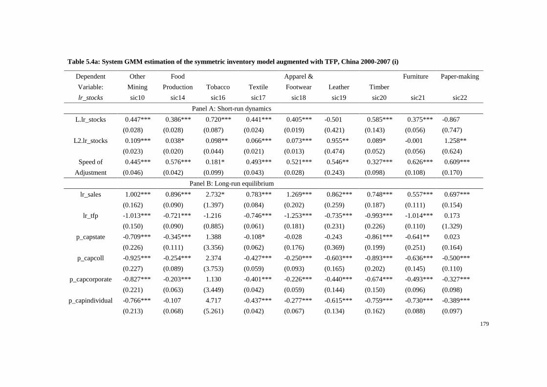
179
Table 5.4a: System GMM estimation of the symmetric inventory model augmented with TFP, China 2000-2007 (i)
Dependent
Variable:
Other
Mining
Food
Production Tobacco Textile
Apparel &
Footwear Leather Timber
Furniture Paper-making
lr_stocks sic10 sic14 sic16 sic17 sic18 sic19 sic20 sic21 sic22
Panel A: Short-run dynamics
L.lr_stocks 0.447*** 0.386*** 0.720*** 0.441*** 0.405*** -0.501 0.585*** 0.375*** -0.867
(0.028) (0.028) (0.087) (0.024) (0.019) (0.421) (0.143) (0.056) (0.747)
L2.lr_stocks 0.109*** 0.038* 0.098** 0.066*** 0.073*** 0.955** 0.089* -0.001 1.258**
(0.023) (0.020) (0.044) (0.021) (0.013) (0.474) (0.052) (0.056) (0.624)
Speed of
Adjustment
0.445*** 0.576*** 0.181* 0.493*** 0.521*** 0.546** 0.327*** 0.626*** 0.609***
(0.046) (0.042) (0.099) (0.043) (0.028) (0.243) (0.098) (0.108) (0.170)
Panel B: Long-run equilibrium
lr_sales 1.002*** 0.896*** 2.732* 0.783*** 1.269*** 0.862*** 0.748*** 0.557*** 0.697***
(0.162) (0.090) (1.397) (0.084) (0.202) (0.259) (0.187) (0.111) (0.154)
lr_tfp -1.013*** -0.721*** -1.216 -0.746*** -1.253*** -0.735*** -0.993*** -1.014*** 0.173
(0.150) (0.090) (0.885) (0.061) (0.181) (0.231) (0.226) (0.110) (1.329)
p_capstate -0.709*** -0.345*** 1.388 -0.108* -0.028 -0.243 -0.861*** -0.641** 0.023
(0.226) (0.111) (3.356) (0.062) (0.176) (0.369) (0.199) (0.251) (0.164)
p_capcoll -0.925*** -0.254*** 2.374 -0.427*** -0.250*** -0.603*** -0.893*** -0.636*** -0.500***
(0.227) (0.089) (3.753) (0.059) (0.093) (0.165) (0.202) (0.145) (0.110)
p_capcorporate -0.827*** -0.203*** 1.130 -0.401*** -0.226*** -0.440*** -0.674*** -0.493*** -0.327***
(0.221) (0.063) (3.449) (0.042) (0.059) (0.144) (0.150) (0.096) (0.098)
p_capindividual -0.766*** -0.107 4.717 -0.437*** -0.277*** -0.615*** -0.759*** -0.730*** -0.389***
(0.213) (0.068) (5.261) (0.042) (0.067) (0.134) (0.162) (0.088) (0.097)
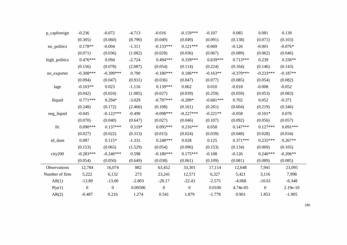
180
p_capforeign -0.236 -0.072 -4.713 -0.016 -0.159*** -0.107 0.085 0.081 0.139
(0.305) (0.060) (8.790) (0.049) (0.049) (0.091) (0.138) (0.071) (0.103)
no_politics 0.178** -0.004 -1.311 -0.133*** 0.121*** -0.069 -0.126 -0.001 -0.076*
(0.071) (0.036) (1.082) (0.028) (0.036) (0.067) (0.089) (0.062) (0.046)
high_politics 0.476*** 0.094 -2.724 0.494*** 0.339*** 0.639*** 0.713*** 0.239 0.336**
(0.156) (0.078) (2.087) (0.054) (0.114) (0.224) (0.164) (0.146) (0.143)
no_exporter -0.308*** -0.399*** 0.790 -0.180*** 0.186*** -0.163** -0.379*** -0.233*** -0.187**
(0.094) (0.047) (0.931) (0.036) (0.047) (0.077) (0.085) (0.054) (0.082)
lage -0.103** 0.023 -1.116 0.139*** 0.062 0.010 -0.018 -0.008 -0.052
(0.042) (0.024) (1.085) (0.027) (0.039) (0.259) (0.059) (0.053) (0.083)
lliquid 0.771*** 0.294* -3.029 -0.797*** -0.289* -0.681*** 0.702 0.052 -0.371
(0.248) (0.172) (2.466) (0.108) (0.161) (0.261) (0.604) (0.219) (0.346)
neg_liquid -0.045 -0.122*** -0.490 -0.098*** -0.227*** -0.221** -0.058 -0.101* 0.076
(0.070) (0.040) (0.647) (0.027) (0.046) (0.107) (0.092) (0.056) (0.057)
lfc 0.090*** 0.137*** 0.519* 0.095*** 0.216*** 0.058 0.147*** 0.127*** 0.091***
(0.027) (0.022) (0.313) (0.015) (0.024) (0.039) (0.048) (0.028) (0.034)
rd_dum 0.087 0.115* -1.331 0.248*** 0.028 0.125 0.371*** 0.235*** 0.267**
(0.153) (0.065) (1.529) (0.054) (0.096) (0.153) (0.134) (0.069) (0.105)
city200 -0.283*** -0.240*** 0.598 -0.180*** 0.175*** -0.108 -0.126 0.246*** -0.206**
(0.054) (0.050) (0.649) (0.038) (0.061) (0.109) (0.081) (0.089) (0.085)
Observations 12,784 16,074 882 63,452 33,301 17,114 12,648 7,941 23,095
Number of firm 5,222 6,132 273 23,241 12,571 6,327 5,421 3,116 7,998
AR(1) -13.89 -13.00 -2.803 -28.17 -22.43 -2.575 -4.068 -10.61 -6.348
P(ar1) 0 0 0.00506 0 0 0.0100 4.74e-05 0 2.19e-10
AR(2) -0.487 0.216 1.274 0.541 1.879 -1.778 0.901 1.853 -1.905

181
P(ar2) 0.626 0.829 0.203 0.589 0.0602 0.0754 0.367 0.0639 0.0568
Hansen test 4.005 9.968 4.733 1.737 7.786 1.864 7.976 5.471 5.659
P(Hansen) 0.261 0.0761 0.316 0.188 0.0506 0.172 0.0925 0.140 0.129
All estimations are conducted using the Arellano and Bond (1991) system GMM technique. All variables are defined in the main text. The dependent
variable is led by one period. The AR(2) is a test for a second-order serial correlation in the residuals, which is distributed as N(0,1) under the null
hypothesis of no serial correlation.
Standard errors in parentheses; ***p<0.01, **p<0.05, *p<0.1

182
Table 5.4b: System GMM estimation of the symmetric inventory model augmented with TFP, China 2000-2007 (ii)
Dependent
Variable: Printing Culture
Petroleum
Processing Chemical Medical Rubber Plastic
Non-metal
Products
Metal
Products
lr_stocks sic23 sic24 sic25 sic26 sic27 sic29 sic30 sic31 sic34
Panel A: Short-run dynamics
L.lr_stocks 0.295** 0.468*** 0.383** 0.437*** 0.367*** 0.470*** 0.472*** 0.446* -0.835
(0.141) (0.072) (0.178) (0.037) (0.063) (0.055) (0.019) (0.266) (0.778)
L2.lr_stocks -0.097 0.132* 0.091 0.081*** 0.005 0.057 0.084*** 0.297 1.086**
(0.146) (0.075) (0.199) (0.020) (0.055) (0.049) (0.015) (0.211) (0.546)
Speed of
Adjustment
0.801*** 0.400*** 0.526 0.482*** 0.628*** 0.473*** 0.444*** 0.256*** 0.748***
(0.286) (0.144) (0.376) (0.054) (0.115) (0.099) (0.031) (0.074) (0.260)
Panel B: Long-run equilibrium
lr_sales 0.741*** 0.573** 0.915* 0.572** 0.448*** 0.733*** 0.471*** 0.931*** 0.934***
(0.147) (0.224) (0.514) (0.265) (0.060) (0.136) (0.050) (0.124) (0.070)
lr_tfp -0.830*** -0.833*** -0.490*** 6.146 -0.472*** -0.775*** -0.534*** -0.704*** -0.569***
(0.164) (0.260) (0.181) (5.155) (0.031) (0.190) (0.050) (0.056) (0.034)
p_capstate -0.898*** -0.076 -0.388 0.641 -0.284*** -0.358** -0.286*** -0.241* -0.072
(0.277) (0.526) (0.439) (0.758) (0.077) (0.140) (0.102) (0.125) (0.093)
p_capcoll -0.756*** -0.852*** -0.538 -0.423** -0.313*** -0.434*** -0.602*** -0.380*** -0.282***
(0.180) (0.206) (0.619) (0.211) (0.075) (0.136) (0.075) (0.119) (0.073)
p_capcorporate -0.690*** -0.860*** -0.459 -0.166 -0.181*** -0.553*** -0.536*** -0.332*** -0.225***
(0.165) (0.164) (0.417) (0.302) (0.063) (0.106) (0.059) (0.103) (0.074)
p_capindividual -0.913*** -0.929*** -0.328 -0.297 -0.213*** -0.486*** -0.710*** -0.269** -0.323***
(0.163) (0.216) (0.622) (0.272) (0.067) (0.112) (0.057) (0.116) (0.060)

183
p_capforeign -0.130 -0.151 0.403 -0.506 0.192** 0.212* 0.090* 0.109 0.148*
(0.081) (0.117) (0.278) (0.436) (0.077) (0.116) (0.050) (0.112) (0.078)
no_politics -0.043 -0.129* 0.059 -0.278* -0.026 -0.139** -0.044 0.006 0.005
(0.043) (0.075) (0.079) (0.158) (0.028) (0.060) (0.034) (0.048) (0.034)
high_politics 0.295*** -0.108 0.076 0.195 0.186*** 0.353*** 0.482*** 0.228** 0.298***
(0.084) (0.242) (1.041) (0.144) (0.044) (0.110) (0.078) (0.099) (0.074)
no_exporter -0.203*** -0.110 -0.052 -0.471* -0.242*** -0.324*** -0.323*** -0.107* -0.122**
(0.063) (0.089) (0.383) (0.247) (0.048) (0.076) (0.039) (0.057) (0.057)
lage 0.135*** 0.108 0.033 0.478 0.104*** 0.133** 0.044 -0.189*** -0.138***
(0.046) (0.175) (0.189) (0.324) (0.031) (0.063) (0.029) (0.049) (0.047)
lliquid -0.385* -0.538** 0.012 -1.512 0.171 -0.083 -0.681*** 1.313*** -0.395**
(0.218) (0.271) (1.060) (1.130) (0.123) (0.263) (0.132) (0.341) (0.180)
neg_liquid -0.102*** -0.289*** -0.116 0.112 -0.068** -0.111 -0.187*** -0.166** -0.183***
(0.035) (0.097) (0.111) (0.146) (0.034) (0.075) (0.040) (0.084) (0.042)
lfc 0.091*** 0.080 0.172 0.327*** 0.115*** 0.130*** 0.183*** 0.129*** 0.060***
(0.018) (0.053) (0.112) (0.116) (0.013) (0.039) (0.022) (0.022) (0.022)
rd_dum 0.265** 0.426*** 0.040 0.455*** 0.266*** 0.392*** 0.430*** 0.063 0.073
(0.115) (0.096) (0.437) (0.175) (0.037) (0.081) (0.050) (0.075) (0.058)
city200 -0.048 -0.012 0.040 -0.336** -0.067 0.067 -0.067 0.033 -0.083**
(0.093) (0.159) (0.082) (0.151) (0.042) (0.103) (0.063) (0.055) (0.036)
Observations 14,822 8,954 5,141 59,665 16,529 8,253 28,148 66,990 41,781
Number of firm 5,160 3,277 1,988 20,934 5,285 3,086 11,177 23,347 18,214
AR(1) -11.00 -10.83 -7.309 -2.637 -14.03 -9.828 -18.71 -1.368 -5.224
P(ar1) 0 0 0 0.00835 0 0 0 0.171 1.75e-07
AR(2) 0.648 0.365 0.762 -0.552 0.817 0.824 0.751 -0.680 -1.734
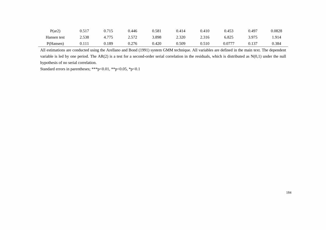
184
P(ar2) 0.517 0.715 0.446 0.581 0.414 0.410 0.453 0.497 0.0828
Hansen test 2.538 4.775 2.572 3.898 2.320 2.316 6.825 3.975 1.914
P(Hansen) 0.111 0.189 0.276 0.420 0.509 0.510 0.0777 0.137 0.384
All estimations are conducted using the Arellano and Bond (1991) system GMM technique. All variables are defined in the main text. The dependent
variable is led by one period. The AR(2) is a test for a second-order serial correlation in the residuals, which is distributed as N(0,1) under the null
hypothesis of no serial correlation.
Standard errors in parentheses; ***p<0.01, **p<0.05, *p<0.1

185
Table 5.4c: System GMM estimation of the symmetric inventory model augmented with TFP, China 2000-2007 (iii)
Dependent
Variable:
Machinery &
Equipment
Transport
Equipment
Measuring
Instrument
Other
Manufacturing
Electronic
Power
Gas
Production
Water
Production
Coal
Mining
lr_stocks sic35 sic37 sic41 sic43 sic44 sic45 sic46 sic60
Panel A: Short-run dynamics
L.lr_stocks 0.453*** 0.775*** 0.421*** 0.348*** 0.491*** 0.262** 0.303*** 0.462***
(0.019) (0.272) (0.055) (0.068) (0.029) (0.110) (0.107) (0.072)
L2.lr_stocks 0.064*** -0.118 -0.003 0.001 0.096*** 0.004 -0.108 0.129*
(0.018) (0.212) (0.039) (0.069) (0.023) (0.097) (0.116) (0.078)
Speed of
Adjustment
0.483*** 0.343*** 0.582*** 0.651*** 0.413*** 0.735*** 0.805*** 0.409***
(0.036) (0.071) (0.090) (0.136) (0.046) (0.193) (0.220) (0.148)
Panel B: Long-run equilibrium
lr_sales 0.459*** 1.345*** 0.590*** 0.348*** 1.214*** 1.284** 0.562*** 0.725**
(0.037) (0.226) (0.074) (0.102) (0.151) (0.499) (0.114) (0.287)
lr_tfp -0.780*** -1.138*** -0.470*** -0.209 -0.668*** -0.771** -0.204*** -0.650**
(0.034) (0.210) (0.054) (0.137) (0.065) (0.342) (0.034) (0.324)
p_capstate -0.494*** 0.031 -0.066 -0.541*** -1.022*** 0.544 0.481 -1.714**
(0.051) (0.215) (0.104) (0.106) (0.299) (0.333) (0.409) (0.774)
p_capcoll -0.751*** -0.410** -0.409*** -0.770*** -0.518 0.714 0.814** -1.987***
(0.048) (0.166) (0.114) (0.081) (0.321) (0.567) (0.329) (0.761)
p_capcorporate -0.652*** -0.425*** -0.284*** -0.740*** -0.972*** 0.455 0.716** -1.903**
(0.038) (0.104) (0.074) (0.057) (0.244) (0.337) (0.358) (0.753)
p_capindividual -0.799*** -0.555*** -0.678*** -0.877*** -0.747** 0.762 0.458 -1.919**
(0.038) (0.126) (0.085) (0.066) (0.297) (0.615) (0.368) (0.749)
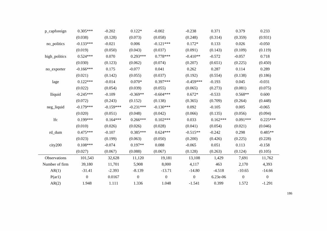
186
p_capforeign 0.305*** -0.202 0.122* -0.002 -0.238 0.371 0.379 0.233
(0.038) (0.128) (0.073) (0.058) (0.248) (0.314) (0.359) (0.931)
no_politics -0.133*** -0.021 0.006 -0.121*** 0.172* 0.133 0.026 -0.050
(0.019) (0.050) (0.043) (0.037) (0.091) (0.143) (0.109) (0.119)
high_politics 0.524*** 0.070 0.293*** 0.778*** -0.410** -0.572 -0.057 0.718
(0.030) (0.123) (0.062) (0.074) (0.207) (0.651) (0.225) (0.450)
no_exporter -0.166*** 0.175 -0.077 0.041 0.262 0.287 0.114 0.289
(0.021) (0.142) (0.055) (0.037) (0.192) (0.554) (0.138) (0.186)
lage 0.122*** -0.014 0.070* 0.397*** -0.459*** -0.193 0.045 -0.031
(0.022) (0.054) (0.039) (0.055) (0.065) (0.273) (0.081) (0.075)
lliquid -0.245*** -0.109 -0.369** -0.604*** 0.672* -0.533 0.568** 0.600
(0.072) (0.243) (0.152) (0.138) (0.365) (0.709) (0.264) (0.448)
neg_liquid -0.179*** -0.159*** -0.231*** -0.130*** 0.092 -0.105 0.005 -0.065
(0.020) (0.051) (0.048) (0.042) (0.066) (0.135) (0.056) (0.094)
lfc 0.199*** 0.164*** 0.266*** 0.102*** 0.033 0.162*** 0.091*** 0.225***
(0.010) (0.026) (0.026) (0.028) (0.041) (0.054) (0.021) (0.046)
rd_dum 0.475*** -0.107 0.385*** 0.624*** -0.515** -0.242 0.298 0.485**
(0.023) (0.199) (0.063) (0.050) (0.200) (0.426) (0.225) (0.228)
city200 0.108*** -0.074 0.197** 0.088 -0.065 0.051 0.113 -0.158
(0.027) (0.067) (0.088) (0.067) (0.128) (0.263) (0.124) (0.105)
Observations 101,543 32,628 11,120 19,181 13,108 1,429 7,691 11,762
Number of firm 39,180 11,701 5,908 8,000 4,117 463 2,170 4,393
AR(1) -31.41 -2.393 -8.139 -13.71 -14.80 -4.518 -10.65 -14.66
P(ar1) 0 0.0167 0 0 0 6.23e-06 0 0
AR(2) 1.948 1.111 1.336 1.048 -1.541 0.399 1.572 -1.291

187
P(ar2) 0.0514 0.267 0.182 0.295 0.123 0.690 0.116 0.197
Hansen test 1.474 5.847 2.731 5.696 7.674 1.159 3.663 2.694
P(Hansen) 0.225 0.119 0.255 0.127 0.104 0.763 0.300 0.260
All estimations are conducted using the Arellano and Bond (1991) system GMM technique. All variables are defined in the main text. The dependent
variable is led by one period. The AR(2) is a test for a second-order serial correlation in the residuals, which is distributed as N(0,1) under the null
hypothesis of no serial correlation.
Standard errors in parentheses; ***p<0.01, **p<0.05, *p<0.1

188
5.5.2 Asymmetric inventory adjustment approach
𝐼𝑖𝑡 = (𝜑1𝐼𝑖,𝑡−1 + 𝜋1′ 𝑋𝑖𝑡) + [(𝜑2 − 𝜑1)𝐼𝑖,𝑡−1 + (𝜋2 − 𝜋1)′𝑋𝑖𝑡]1{𝑞<𝑐} + 𝑣𝑖𝑡 (5.4)
Table 5.5(a), Table5.5(b) and Table5.5(c) present the results from the system GMM
estimation of the threshold partial adjustment model, equation (5.4), and the business
cycle dummy is employed as the transition variable. Firm-years are classified into
down (up) regime when the value of the transition variable equals to one (zero). Panel
A and Panel B focus on samples in the up regime and present the short-run speed of
adjustment towards desired inventory level and the long-run coefficients on the
determinants of target inventory level. Panel C and Panel D contain the deviations
between the two regimes. The AR(2) and Hansen tests are not rejected at the 5%
significance level, suggesting that all GMM regressions use valid instruments.
In terms of the short-term dynamics, the partial adjustment mechanism is captured for
most of the industries in the up regime since the speeds of adjustment are significantly
positive and lower than 1. When allowing for the asymmetric adjustment mechanism,
results in panel C show that the deviations of the speed of adjustment between the two
regimes are significant. They are estimated to be significantly positive for 14 out of 26
industries, which indicate a higher speed of adjustment during economic slowdown.
189
In short-run, firms in the 14 industries spend less time to change their deviation from
target inventory level during business cycle downwards. For example, the speed of
adjustment for the printing industry is 0.523 in the upswing region, and it increases to
0.674 (0.523+0.151) in the downswing region, which means with annual data that 52.3%
[67.4%] of the difference between actual inventory level and the target inventory level
is eliminated in one year in upswing [downswing]. Firms spend 1.912 years (22.944
months) to eliminate the gap in the upswing and 1.484 years (17.808 months) in the
downswing, therefore, firms in printing industry will spend 5.136 months (about 157
days) less to cover the distance to the long-term level during recession.
This could be supported by a number of studies suggesting that, with a low adjustment
cost, inventories are likely to be quite sensitive to business environment under
imperfect capital markets (Sangalli, 2013, Guariglia, 2000, Guariglia and Mateut,
2006).
However, the deviations of the speed of adjustment are negatively significant for other
11 industries (e.g. Machinery & equipment industry, electronic power industry and
other manufacturing industry). Firms in these industries usually have high adjustment
costs and therefore, the speed of adjustment is relatively low even for firms in the up
regime. During the recession, these firms tend to have a higher level of financial

190
constraint and cannot afford the adjustment cost, thus, become less sensitive to demand
shocks.
In terms of long-run results, same as the symmetric analysis, when compared with the
results in Table 4.4, including TFP into the equation makes the estimated coefficient
of sales decreased considerably in the two regimes for the majority of industries. When
focusing on TFP, firms in the up regime tend to have significantly negative coefficients
of TFP for most of the industries (23 out of 26), which indicates the inventory reducing
impact of TFP. Outcomes in Panel C show that the deviations of TFP coefficient
between the two regimes are not as obvious as that of adjustment speed in short-run
perspective. This finding illustrates that the inventory reducing impact of TFP is not
sensitive to macroeconomic fluctuation. In other words, the negative impact of
business cycle downwards does not offset the benefits associated with the product and
process innovations.
Moreover, for industries such as tobacco and printing, the inventory reducing impact
of TFP becomes clear during recessions. In the up regime, the coefficient of TFP is
not significant for the tobacco and printing industries, which represents that a growth
of TFP does not result in a drop of inventory volume. According to Panel D, the
deviation of TFP’s coefficient between up regime and down regime is significantly
negative for the two industries. More specifically, for firms in the tobacco industry and

191
printing industry, each percentage of TFP growth results in 0.236% and 0.628% of
inventory reduction respectively, during the downward business cycle. One reasonable
explanation could be that firms in these consumer non-durable industries tend to adopt
the wait-and-see strategy in the period of recession and a higher level of productivity
could help firms in these industries get a better inventory performance.

192
Table 5.5a: System GMM estimation of the asymmetric threshold model augmented with TFP, China 2000-2007 (i)
Dependent
Variable:
Other
Mining
Food
Production
Tobacco
Textile
Apparel &
Footwear
Leather
Timber
Furniture Paper-
making
lr_stocks sic10 sic14 sic16 sic17 sic18 sic19 sic20 sic21 sic22
Panel A: Short-run dynamics
Speed of
Adjustment
0.432*** 0.570*** 0.305*** 0.424*** 0.519*** 0.264 0.385*** 0.381*** 0.317***
(0.042) (0.041) (0.104) (0.032) (0.029) (0.197) (0.086) (0.077) (0.104)
Panel B: Long-run equilibrium
lr_sales 0.925** 1.039*** 1.111*** 0.896*** 1.286*** 1.168* 0.679*** 0.793*** 0.921***
(0.435) (0.121) (0.385) (0.101) (0.194) (0.672) (0.211) (0.191) (0.224)
lr_tfp -0.903** -0.902*** -0.163 -0.860*** -1.289*** -1.773 -0.947*** -1.243*** -3.982
(0.406) (0.137) (0.304) (0.118) (0.251) (1.160) (0.253) (0.201) (2.550)
p_capstate -0.639** -0.236 -0.221 -0.153 0.074 0.175 -1.005*** -0.846** -1.073*
(0.283) (0.182) (2.938) (0.114) (0.220) (0.726) (0.256) (0.423) (0.647)
p_capcoll -0.900*** -0.203 -0.414 -0.313** -0.218* -0.442 -1.136*** -0.469 -1.006**
(0.301) (0.149) (2.896) (0.123) (0.120) (0.477) (0.229) (0.331) (0.394)
p_capcorporate -0.754*** -0.208** -0.668 -0.322*** -0.222*** -0.261 -0.827*** -0.253 -0.781**
(0.266) (0.100) (2.962) (0.086) (0.081) (0.432) (0.150) (0.185) (0.325)
p_capindividual -0.771*** -0.055 0.462 -0.314*** -0.314*** -0.321 -0.946*** -0.515*** -0.720**
(0.298) (0.115) (3.041) (0.090) (0.086) (0.425) (0.157) (0.160) (0.327)
p_capforeign -0.466 -0.159* -2.873 0.208** -0.136** -0.004 0.018 0.036 -0.252
(0.389) (0.096) (3.841) (0.099) (0.067) (0.297) (0.168) (0.146) (0.259)
no_politics 0.219* 0.085 -0.438 -0.107** 0.153*** -0.216 0.061 0.108 -0.216*

193
(0.116) (0.059) (0.661) (0.049) (0.051) (0.162) (0.118) (0.131) (0.121)
high_politics 0.658** 0.186* -0.818 0.565*** 0.563*** 0.238 0.956*** 0.591* 0.713**
(0.311) (0.112) (0.810) (0.092) (0.153) (0.595) (0.216) (0.328) (0.303)
no_exporter -0.331* -0.393*** -0.376 -0.120** 0.186*** -0.312 -0.351*** -0.361*** -0.430**
(0.173) (0.072) (0.464) (0.053) (0.058) (0.229) (0.088) (0.118) (0.219)
lage -0.091 0.042 -0.260 0.179*** 0.048 0.021 0.070 -0.182* -0.520**
(0.082) (0.035) (0.379) (0.034) (0.043) (0.350) (0.060) (0.098) (0.216)
lliquid 0.866* 0.488* -1.659 -0.829*** -0.162 -0.620 0.382 0.107 -0.093
(0.446) (0.291) (1.213) (0.208) (0.238) (1.116) (0.437) (0.427) (0.532)
neg_liquid 0.027 -0.128** -0.056 -0.085* -0.206*** -0.390 -0.066 -0.199 -0.235
(0.097) (0.063) (0.353) (0.049) (0.061) (0.413) (0.103) (0.128) (0.209)
lfc 0.103** 0.141*** 0.324* 0.145*** 0.174*** 0.118 0.105** 0.199*** 0.015
(0.052) (0.031) (0.173) (0.025) (0.029) (0.110) (0.048) (0.058) (0.110)
rd_dum 0.115 0.050 0.835 0.075 -0.039 -0.066 0.298 0.158 0.218
(0.448) (0.099) (0.598) (0.088) (0.130) (0.344) (0.188) (0.149) (0.194)
city200 -0.336*** -0.283*** 0.591 -0.014 0.032 -0.166 -0.120 0.062 -0.395**
(0.070) (0.062) (0.395) (0.073) (0.089) (0.519) (0.090) (0.153) (0.177)
Effects of the business cycle dummy variable:
Panel C: Short-run dynamics
Speed of
Adjustment’
0.008*** -0.004*** -0.032*** 0.019*** -0.014*** 0.078*** -0.022*** -0.019*** 0.020***
(0.007) (0.007) (0.028) (0.012) (0.010) (0.071) (0.009) (0.009) (0.024)
Panel D: Long-run equilibrium
lr_sales’ 0.067 -0.138 0.229** -0.103 0.014 -0.165 0.002 0.070 0.058
(0.480) (0.106) (0.099) (0.063) (0.165) (0.268) (0.103) (0.047) (0.091)
lr_tfp’ -0.106 0.170 -0.236* 0.052 0.008 0.348 0.046 -0.018 0.846

194
(0.453) (0.123) (0.123) (0.067) (0.222) (0.312) (0.103) (0.053) (0.643)
p_capstate’ -0.088 -0.100 0.194 0.001 -0.062 -0.226 0.113 0.497*** 0.459
(0.147) (0.156) (0.509) (0.062) (0.164) (0.376) (0.120) (0.178) (0.290)
p_capcoll’ -0.041 -0.044 0.492 -0.095 -0.008 -0.140 0.161 0.078 0.263
(0.148) (0.118) (0.524) (0.071) (0.097) (0.266) (0.117) (0.149) (0.197)
p_capcorporate’ -0.089 0.002 0.379 -0.048 0.009 -0.061 0.104 -0.006 0.234
(0.137) (0.075) (0.544) (0.046) (0.063) (0.198) (0.069) (0.071) (0.158)
p_capindividual’ -0.023 -0.049 0.162 -0.081 0.051 -0.146 0.111 0.002 0.180
(0.151) (0.095) (0.853) (0.052) (0.075) (0.190) (0.072) (0.065) (0.161)
p_capforeign’ 0.207 0.079 -0.672 -0.127*** -0.014 -0.036 0.039 0.037 0.149
(0.199) (0.055) (4.105) (0.049) (0.047) (0.084) (0.088) (0.071) (0.135)
no_politics’ -0.029 -0.088** -0.034 -0.009 -0.035 0.019 -0.106** 0.008 0.057
(0.077) (0.043) (0.268) (0.025) (0.034) (0.059) (0.052) (0.058) (0.047)
high_politics’ -0.154 -0.093 -0.068 -0.038 -0.209** 0.120 -0.157 -0.206 -0.154*
(0.353) (0.059) (0.220) (0.042) (0.092) (0.175) (0.108) (0.145) (0.093)
no_exporter’ 0.030 -0.001 0.208 -0.065* 0.012 0.004 0.008 0.084 0.159
(0.166) (0.055) (0.159) (0.034) (0.045) (0.093) (0.047) (0.057) (0.114)
Lage’ -0.013 -0.022 0.006 -0.031*** 0.004 -0.035 -0.053* 0.026 0.155
(0.057) (0.023) (0.096) (0.012) (0.022) (0.089) (0.029) (0.036) (0.098)
Lliquid’ -0.065 -0.189 -0.316 -0.030 -0.082 -0.291 0.087 0.210 0.226
(0.423) (0.254) (0.612) (0.126) (0.212) (0.575) (0.180) (0.193) (0.221)
neg_liquid’ -0.064 0.003 -0.188 -0.019 -0.012 -0.046 0.012 0.019 0.091
(0.064) (0.046) (0.177) (0.027) (0.048) (0.150) (0.052) (0.057) (0.092)
lfc’ -0.011 -0.008 -0.027 -0.033** 0.033* 0.005 0.016 -0.029 0.029
(0.031) (0.020) (0.076) (0.013) (0.017) (0.030) (0.024) (0.027) (0.038)

195
rd_dum’ -0.010 0.064 -0.541** 0.153*** 0.042 0.116 0.035 -0.019 0.003
(0.493) (0.091) (0.242) (0.055) (0.100) (0.176) (0.098) (0.073) (0.082)
city200’ 0.050 0.047 -0.216 -0.119*** 0.143** 0.005 0.027 0.063 0.131
(0.054) (0.036) (0.141) (0.042) (0.064) (0.189) (0.041) (0.072) (0.099)
Observations 12,784 16,074 882 63,452 33,301 17,114 12,648 7,941 23,095
Number of firm 5,222 6,132 273 23,241 12,571 6,327 5,421 3,116 7,998
AR(1) -13.90 -13.07 -2.904 -28.62 -2.153 -2.213 -4.272 -10.54 -1.653
P(ar1) 0 0 0.00368 0 0.0313 0.0269 1.94e-05 0 0.0983
AR(2) -0.513 0.119 1.501 -0.0806 1.147 -1.238 0.555 1.518 -1.182
P(ar2) 0.608 0.905 0.133 0.936 0.251 0.216 0.579 0.129 0.237
Hansen test 6.374 7.893 12.57 3.568 4.376 2.619 7.246 3.024 7.723
P(Hansen) 0.383 0.639 0.127 0.168 0.112 0.106 0.510 0.0820 0.259
All estimations are conducted using the Arellano and Bond (1991) system GMM technique. All variables are defined in the main text. The dependent
variable is led by one period. The AR(2) is a test for a second-order serial correlation in the residuals, which is distributed as N(0,1) under the null
hypothesis of no serial correlation.
Standard errors in parentheses; ***p<0.01, **p<0.05, *p<0.1

196
Table 5.5b: System GMM estimation of the asymmetric threshold model augmented with TFP, China 2000-2007 (ii)
Dependent
Variable: Printing Culture
Petroleum
Processing Chemical Medical Rubber Plastic
Non-metal
Products
Metal
Products
lr_stocks sic23 sic24 sic25 sic26 sic27 sic29 sic30 sic31 sic34
Panel A: Short-run dynamics
Speed of
Adjustment
0.523*** 0.201** 0.248* 0.548*** 0.525*** 0.372*** 0.405*** 0.239** 0.227
(0.113) (0.083) (0.135) (0.023) (0.123) (0.092) (0.029) (0.097) (0.166)
Panel B: Long-run equilibrium
lr_sales 0.483* 1.299** 1.957** 0.910*** 0.497*** 0.830*** 0.465*** 0.171 0.948***
(0.266) (0.629) (0.917) (0.042) (0.159) (0.270) (0.065) (0.218) (0.235)
lr_tfp -0.359 -2.064** -0.815*** -2.089*** -0.510*** -0.876** -0.496*** -0.367*** -0.684***
(0.375) (0.865) (0.314) (0.521) (0.087) (0.389) (0.061) (0.102) (0.162)
p_capstate -1.873*** 1.357 1.114 -0.698*** -0.333* -0.102 -0.148 -1.142*** -0.457
(0.549) (1.343) (1.286) (0.206) (0.187) (0.244) (0.139) (0.375) (0.410)
p_capcoll -1.512*** -0.717 0.913 -0.848*** -0.344** -0.231 -0.581*** -1.097*** -0.501*
(0.380) (0.544) (1.465) (0.148) (0.175) (0.276) (0.107) (0.315) (0.264)
p_capcorporate -1.432*** -0.138 0.767 -0.742*** -0.213 -0.384* -0.549*** -0.765*** -0.551**
(0.356) (0.575) (1.115) (0.130) (0.140) (0.202) (0.088) (0.232) (0.274)
p_capindividual -1.606*** 0.182 1.490 -0.809*** -0.258 -0.330 -0.681*** -0.892*** -0.430*
(0.354) (0.744) (1.589) (0.131) (0.180) (0.217) (0.082) (0.277) (0.237)
p_capforeign -0.501** 0.115 1.069 0.028 0.142 0.136 0.062 -0.282 0.012
(0.242) (0.334) (0.848) (0.093) (0.119) (0.197) (0.074) (0.229) (0.206)
no_politics -0.059 -0.391 0.108 -0.036 0.004 0.086 -0.083 0.034 -0.067

197
(0.077) (0.251) (0.231) (0.031) (0.067) (0.146) (0.052) (0.086) (0.125)
high_politics 0.435** 0.712 -1.704 0.346*** 0.224*** 0.273 0.465*** 0.835*** 0.341*
(0.188) (0.457) (1.625) (0.067) (0.059) (0.175) (0.096) (0.229) (0.175)
no_exporter -0.686*** -0.031 0.688 -0.171*** -0.244* -0.363** -0.327*** -0.537*** -0.197
(0.200) (0.263) (0.766) (0.042) (0.145) (0.141) (0.060) (0.146) (0.167)
lage 0.126** -0.468 -0.218 -0.056 0.091** 0.092 0.033 -0.195*** -0.321
(0.050) (0.439) (0.283) (0.055) (0.043) (0.093) (0.043) (0.075) (0.200)
lliquid -1.891*** 0.339 1.492 0.038 0.231 0.212 -0.792*** -0.275 -0.414
(0.658) (0.906) (1.613) (0.130) (0.313) (0.525) (0.201) (0.488) (0.538)
neg_liquid -0.281*** -0.435* 0.082 -0.137** -0.067 -0.175 -0.249*** -0.299** -0.258**
(0.099) (0.249) (0.256) (0.057) (0.086) (0.116) (0.061) (0.142) (0.117)
lfc 0.125*** 0.341* 0.447* 0.136*** 0.109*** 0.191*** 0.236*** 0.085** 0.001
(0.037) (0.176) (0.233) (0.036) (0.021) (0.065) (0.032) (0.035) (0.081)
rd_dum 0.963*** -0.169 -0.912 0.231*** 0.297*** 0.427*** 0.340*** 0.650*** 0.328
(0.303) (0.393) (0.837) (0.037) (0.098) (0.155) (0.075) (0.214) (0.245)
city200 -0.023 -0.352 -0.172 -0.135** -0.071 0.143 0.045 -0.027 -0.244*
(0.143) (0.386) (0.242) (0.054) (0.054) (0.140) (0.093) (0.134) (0.146)
Effects of the business cycle dummy variable:
Panel C: Short-run dynamics
Speed of
Adjustment’
0.151*** 0.001*** 0.042*** -0.006*** 0.000 0.001*** -0.013*** -0.047*** 0.019***
(0.075) (0.012) (0.024) (0.004) (0.160) (0.010) (0.007) (0.041) (0.014)
Panel D: Long-run equilibrium
lr_sales’ 0.414** -0.061 -0.145** 0.005 -0.058 0.004 0.005 0.395*** 0.061
(0.187) (0.075) (0.067) (0.028) (0.172) (0.153) (0.036) (0.139) (0.086)
lr_tfp’ -0.628** 0.165 -0.007 0.298 0.043 -0.001 -0.039 -0.140*** -0.023

198
(0.281) (0.113) (0.032) (0.252) (0.090) (0.232) (0.043) (0.051) (0.020)
p_capstate’ 0.985** -0.039 -0.413** 0.164 0.044 -0.182 -0.086 0.424*** -0.007
(0.411) (0.174) (0.173) (0.156) (0.181) (0.113) (0.080) (0.158) (0.094)
p_capcoll’ 0.658*** 0.039 -0.392** 0.147 0.028 -0.077 0.004 0.331** -0.005
(0.251) (0.113) (0.200) (0.123) (0.149) (0.119) (0.056) (0.133) (0.140)
p_capcorporate’ 0.620*** -0.140 -0.356** 0.121 0.047 -0.087 0.034 0.203** 0.032
(0.235) (0.086) (0.163) (0.110) (0.117) (0.082) (0.045) (0.095) (0.094)
p_capindividual’ 0.570** -0.197** -0.490*** 0.106 0.076 -0.051 0.011 0.310*** 0.018
(0.236) (0.082) (0.166) (0.110) (0.140) (0.085) (0.042) (0.112) (0.122)
p_capforeign’ 0.277* -0.052 -0.198 0.101 0.056 0.059 0.011 0.114 0.010
(0.154) (0.072) (0.190) (0.063) (0.076) (0.087) (0.038) (0.072) (0.091)
no_politics’ 0.033 0.061 -0.013 -0.002 -0.023 -0.122** 0.035 0.008 0.018
(0.043) (0.053) (0.067) (0.022) (0.045) (0.053) (0.026) (0.031) (0.029)
high_politics’ -0.221* -0.439*** 0.194 -0.016 -0.050 0.033 -0.014 -0.324*** -0.050
(0.125) (0.157) (0.145) (0.038) (0.034) (0.079) (0.046) (0.095) (0.070)
no_exporter’ 0.415*** 0.011 -0.129 0.047 -0.008 0.041 0.003 0.189*** 0.061
(0.142) (0.060) (0.117) (0.033) (0.161) (0.094) (0.033) (0.056) (0.068)
Lage’ 0.002 0.038 -0.003 0.040 -0.003 -0.013 -0.011 0.007 0.017
(0.028) (0.036) (0.036) (0.041) (0.023) (0.032) (0.020) (0.014) (0.024)
Lliquid’ 1.289*** -0.232 -0.014 0.146 -0.022 -0.149 0.086 0.729*** 0.209
(0.498) (0.202) (0.292) (0.090) (0.259) (0.251) (0.109) (0.247) (0.176)
neg_liquid’ 0.164** 0.010 -0.108 0.034 -0.013 -0.003 0.034 0.042 -0.033
(0.071) (0.060) (0.070) (0.043) (0.091) (0.047) (0.031) (0.036) (0.057)
lfc’ -0.012 -0.060** -0.065* 0.010 0.010 -0.036 -0.033** 0.006 0.035
(0.019) (0.031) (0.036) (0.025) (0.018) (0.025) (0.015) (0.011) (0.030)

199
rd_dum’ -0.540*** 0.165** 0.180 -0.007 -0.015 -0.023 0.062 -0.302*** -0.066
(0.203) (0.075) (0.119) (0.026) (0.113) (0.100) (0.040) (0.088) (0.095)
city200’ 0.024 0.024 0.107 0.015 0.007 -0.036 -0.071 0.019 0.058
(0.070) (0.071) (0.070) (0.044) (0.028) (0.069) (0.046) (0.031) (0.043)
Observations 14,822 8,954 5,141 59,665 16,529 8,253 28,148 66,990 41,781
Number of firm 5,160 3,277 1,988 20,934 5,285 3,086 11,177 23,347 18,214
AR(1) -12.78 -10.27 -8.445 -2.653 -14.42 -10.18 -8.061 -2.238 -3.191
P(ar1) 0 0 0 0.00797 0 0 0 0.0252 0.00142
AR(2) -1.454 0.494 0.101 -0.608 -0.0309 0.0938 -1.642 0.392 -1.889
P(ar2) 0.146 0.621 0.920 0.543 0.975 0.925 0.101 0.695 0.0589
Hansen test 2.329 4.613 2.375 7.443 7.271 4.491 5.276 2.835 2.983
P(Hansen) 0.312 0.0996 0.667 0.114 0.296 0.611 0.153 0.586 0.225
All estimations are conducted using the Arellano and Bond (1991) system GMM technique. All variables are defined in the main text. The dependent
variable is led by one period. The AR(2) is a test for a second-order serial correlation in the residuals, which is distributed as N(0,1) under the null
hypothesis of no serial correlation.
Standard errors in parentheses; ***p<0.01, **p<0.05, *p<0.1

200
Table 5.5c: System GMM estimation of the asymmetric threshold model augmented with TFP, China 2000-2007 (iii)
Dependent
Variable:
Machinery &
Equipment
Transport
Equipment
Measuring
Instrument
Other
Manufacturing
Electronic
Power
Gas
Production
Water
Production
Coal
Mining
lr_stocks sic35 sic37 sic41 sic43 sic44 sic45 sic46 sic60
Panel A: Short-run dynamics
Speed of
Adjustment
0.188*** 0.371*** 0.349*** 0.284*** 0.337*** 0.755*** 0.674*** 0.320***
(0.019) (0.045) (0.053) (0.054) (0.041) (0.151) (0.158) (0.095)
Panel B: Long-run equilibrium
lr_sales 1.497*** 1.334*** 0.588*** 0.567** 1.560*** 1.173*** 0.642*** 2.283***
(0.235) (0.138) (0.106) (0.223) (0.181) (0.404) (0.111) (0.782)
lr_tfp -1.560*** -1.151*** -0.568*** -0.621* -0.718*** -0.768** -0.183*** -2.482***
(0.185) (0.128) (0.088) (0.355) (0.079) (0.305) (0.043) (0.912)
p_capstate 0.912** 0.006 -0.107 -0.364 -0.235 0.610* 0.852 -0.911
(0.364) (0.144) (0.171) (0.224) (0.428) (0.364) (0.615) (1.225)
p_capcoll 0.659* -0.551*** -0.457** -0.808*** -0.248 0.550 1.128** -1.436
(0.361) (0.125) (0.203) (0.185) (0.493) (0.605) (0.542) (1.213)
p_capcorporate 0.416 -0.513*** -0.310** -0.750*** -0.425 0.743** 0.997* -1.760
(0.289) (0.103) (0.121) (0.143) (0.358) (0.366) (0.573) (1.175)
p_capindividual 0.549* -0.670*** -0.708*** -0.753*** -0.117 1.060* 0.576 -1.257
(0.334) (0.099) (0.132) (0.147) (0.437) (0.628) (0.580) (1.215)
p_capforeign 0.384*** -0.245** 0.098 -0.033 -0.159 0.782** 0.308 -2.923
(0.128) (0.119) (0.121) (0.135) (0.337) (0.378) (0.777) (2.271)
no_politics 0.278** -0.128** 0.021 -0.103 0.300** -0.055 0.087 0.264

201
(0.115) (0.055) (0.082) (0.088) (0.151) (0.189) (0.150) (0.241)
high_politics 0.174 0.072 0.195* 0.830*** -0.800*** -0.182 -0.231 -1.689
(0.130) (0.089) (0.114) (0.136) (0.251) (0.574) (0.351) (1.263)
no_exporter 0.284* 0.132 -0.083 0.015 0.576 -0.004 0.465 0.791**
(0.150) (0.096) (0.097) (0.092) (0.516) (0.669) (0.745) (0.325)
lage -0.321*** -0.058 -0.052 0.130 -0.556*** -0.159 -0.028 -0.352*
(0.101) (0.053) (0.064) (0.103) (0.092) (0.255) (0.099) (0.196)
lliquid 1.492*** 0.085 -0.740** -0.770** 1.263** -1.024 1.121*** 1.265
(0.481) (0.222) (0.288) (0.384) (0.609) (0.869) (0.423) (0.836)
neg_liquid -0.002 -0.120* -0.295*** -0.233** 0.005 -0.154 0.092 -0.101
(0.090) (0.064) (0.092) (0.111) (0.128) (0.205) (0.084) (0.196)
lfc 0.272*** 0.178*** 0.267*** 0.271*** 0.111 0.120** 0.083*** 0.168**
(0.032) (0.029) (0.044) (0.071) (0.071) (0.051) (0.026) (0.073)
rd_dum -0.240 -0.127 0.376*** 0.760*** -0.970*** -0.221 0.418* -0.051
(0.205) (0.122) (0.110) (0.137) (0.276) (0.359) (0.215) (0.507)
city200 0.430*** -0.049 0.097 0.139 -0.361** 0.073 0.024 -0.695**
(0.112) (0.067) (0.129) (0.128) (0.172) (0.262) (0.127) (0.276)
Effects of the business cycle dummy variable
Panel C: Short-run dynamics
Speed of
Adjustment’
-0.082*** 0.012*** 0.003*** -0.002*** -0.003*** 0.011*** 0.007*** 0.032***
(0.021) (0.011) (0.007) (0.006) (0.006) (0.019) (0.005) (0.009)
Panel D: Long-run equilibrium
lr_sales’ -0.157*** -0.026 0.107 0.172* 0.018 0.085 -0.017 -0.590***
(0.027) (0.065) (0.069) (0.095) (0.025) (0.149) (0.055) (0.179)
lr_tfp’ 0.144*** 0.050 -0.017 -0.158 -0.038* 0.050 -0.032 0.704***
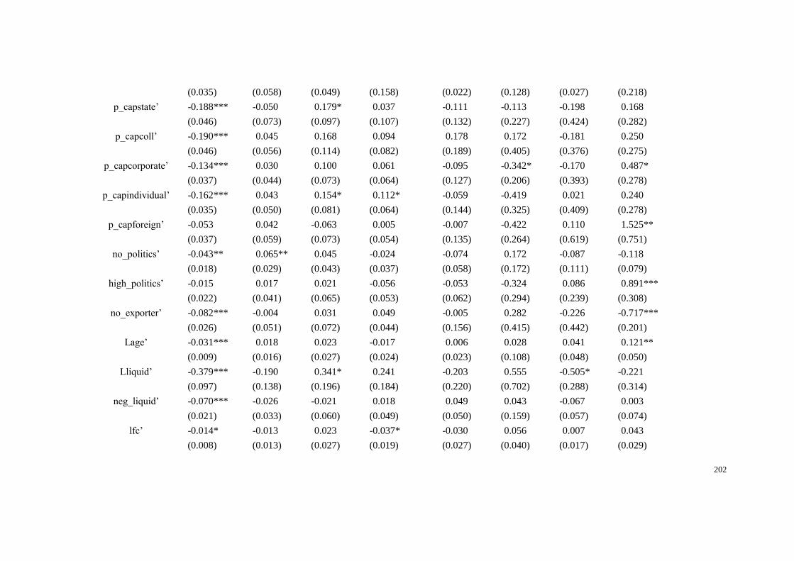
202
(0.035) (0.058) (0.049) (0.158) (0.022) (0.128) (0.027) (0.218)
p_capstate’ -0.188*** -0.050 0.179* 0.037 -0.111 -0.113 -0.198 0.168
(0.046) (0.073) (0.097) (0.107) (0.132) (0.227) (0.424) (0.282)
p_capcoll’ -0.190*** 0.045 0.168 0.094 0.178 0.172 -0.181 0.250
(0.046) (0.056) (0.114) (0.082) (0.189) (0.405) (0.376) (0.275)
p_capcorporate’ -0.134*** 0.030 0.100 0.061 -0.095 -0.342* -0.170 0.487*
(0.037) (0.044) (0.073) (0.064) (0.127) (0.206) (0.393) (0.278)
p_capindividual’ -0.162*** 0.043 0.154* 0.112* -0.059 -0.419 0.021 0.240
(0.035) (0.050) (0.081) (0.064) (0.144) (0.325) (0.409) (0.278)
p_capforeign’ -0.053 0.042 -0.063 0.005 -0.007 -0.422 0.110 1.525**
(0.037) (0.059) (0.073) (0.054) (0.135) (0.264) (0.619) (0.751)
no_politics’ -0.043** 0.065** 0.045 -0.024 -0.074 0.172 -0.087 -0.118
(0.018) (0.029) (0.043) (0.037) (0.058) (0.172) (0.111) (0.079)
high_politics’ -0.015 0.017 0.021 -0.056 -0.053 -0.324 0.086 0.891***
(0.022) (0.041) (0.065) (0.053) (0.062) (0.294) (0.239) (0.308)
no_exporter’ -0.082*** -0.004 0.031 0.049 -0.005 0.282 -0.226 -0.717***
(0.026) (0.051) (0.072) (0.044) (0.156) (0.415) (0.442) (0.201)
Lage’ -0.031*** 0.018 0.023 -0.017 0.006 0.028 0.041 0.121**
(0.009) (0.016) (0.027) (0.024) (0.023) (0.108) (0.048) (0.050)
Lliquid’ -0.379*** -0.190 0.341* 0.241 -0.203 0.555 -0.505* -0.221
(0.097) (0.138) (0.196) (0.184) (0.220) (0.702) (0.288) (0.314)
neg_liquid’ -0.070*** -0.026 -0.021 0.018 0.049 0.043 -0.067 0.003
(0.021) (0.033) (0.060) (0.049) (0.050) (0.159) (0.057) (0.074)
lfc’ -0.014* -0.013 0.023 -0.037* -0.030 0.056 0.007 0.043
(0.008) (0.013) (0.027) (0.019) (0.027) (0.040) (0.017) (0.029)
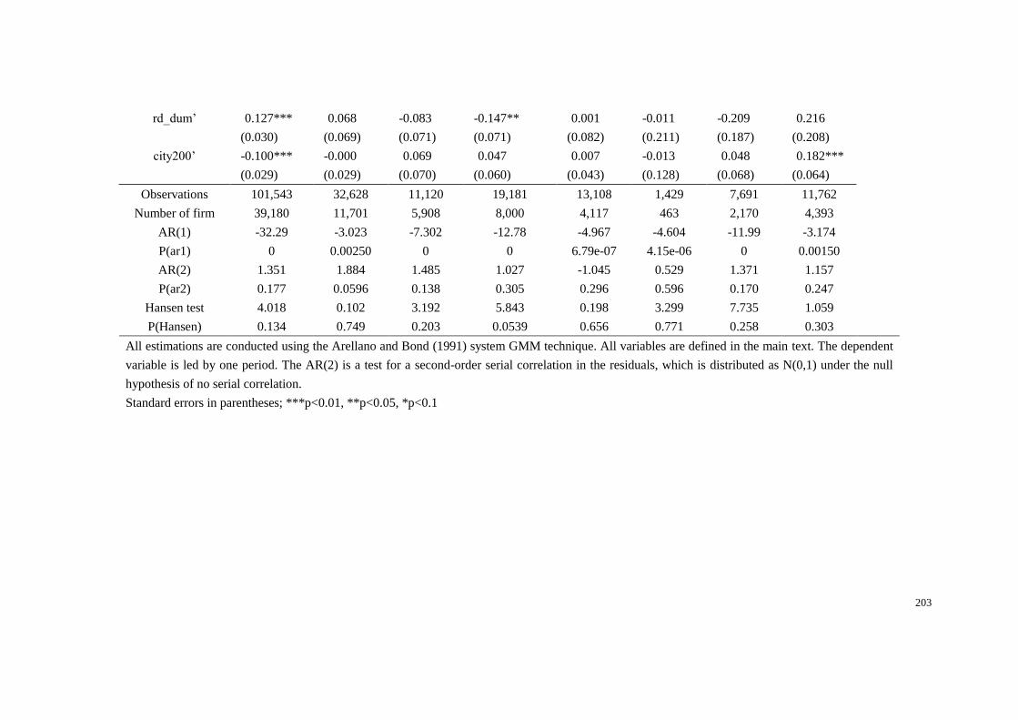
203
rd_dum’ 0.127*** 0.068 -0.083 -0.147** 0.001 -0.011 -0.209 0.216
(0.030) (0.069) (0.071) (0.071) (0.082) (0.211) (0.187) (0.208)
city200’ -0.100*** -0.000 0.069 0.047 0.007 -0.013 0.048 0.182***
(0.029) (0.029) (0.070) (0.060) (0.043) (0.128) (0.068) (0.064)
Observations 101,543 32,628 11,120 19,181 13,108 1,429 7,691 11,762
Number of firm 39,180 11,701 5,908 8,000 4,117 463 2,170 4,393
AR(1) -32.29 -3.023 -7.302 -12.78 -4.967 -4.604 -11.99 -3.174
P(ar1) 0 0.00250 0 0 6.79e-07 4.15e-06 0 0.00150
AR(2) 1.351 1.884 1.485 1.027 -1.045 0.529 1.371 1.157
P(ar2) 0.177 0.0596 0.138 0.305 0.296 0.596 0.170 0.247
Hansen test 4.018 0.102 3.192 5.843 0.198 3.299 7.735 1.059
P(Hansen) 0.134 0.749 0.203 0.0539 0.656 0.771 0.258 0.303
All estimations are conducted using the Arellano and Bond (1991) system GMM technique. All variables are defined in the main text. The dependent
variable is led by one period. The AR(2) is a test for a second-order serial correlation in the residuals, which is distributed as N(0,1) under the null
hypothesis of no serial correlation.
Standard errors in parentheses; ***p<0.01, **p<0.05, *p<0.1
204
5.6 Conclusions
In this chapter, we supplied a study of the relationship between TFP and inventory
performance in order to test the impact of innovation, especially the efficiency
innovation, on inventory management. Generally speaking, TFP, as a proxy for firm’s
productivity, is detected to be a superior measurement of inventory management
innovation since it captures both technological progress and technical efficiency
change. The augment of TFP into the variant error-correction model increases the
reliability of the estimations.
Our results suggest that the inventory reducing impact of TFP is significant for most
of the industries. It states that firms with more product innovation are more capable of
matching their production and inventory with demand over product life cycles, which
leads to a more efficient inventory management. Moreover, an efficient production
process reduces flow time and lead time, which allows firms eliminate waste, lower
the reorder point and reduce safety inventory. All these benefits contribute to a lower
inventory volume.
When allowing the asymmetric mechanism, we find that, same as other variables that
determine long-run target inventory level, TFP works symmetrically between the

205
upswing and downswing of business cycle, which means the benefits of productivity
improvement are stable and cannot be discharged by adverse economic environment.

206
Chapter 6. Overall Conclusion
207
Chapter 6: Overall Conclusion
6.1 Introduction
This doctoral thesis examines the inventory management and performance in China.
Numerous investigations acknowledge that inventory plays an essential role in the
provision of products and services at all levels of an economy, and inventory
management and its development have complex impacts on firm’s performance.
However, the literature lacks evidence to understand the industry heterogeneity in
inventory control. In this thesis, an extensive review of the literature led us to seek to
investigate firm’ inventory management behaviour under different economic condition.
This is done by adopting a regime-switching transition variable and analysing the
error-correction model allowing an asymmetric adjustment mechanism. Moreover,
following the study of TFP growth in China (Ding et al., 2014), this research attempts
to uncover the relationship between innovation and inventory performance through
examining TFP’s inventory reducing impact.
This thesis has six chapters. The first chapter provides an overview of the research
background, objectives, database, and contributions of this doctoral thesis. In Chapter
2, we supplied a literature review on the relationships between inventory management
208
and firm’s exogenous and endogenous factors, as well as the development of inventory
control and the discussion of their influences on firm’s performance. Chapter 3 is
devoted to analysing firm’s inventory adjustment pattern in short-run and the
determinants of firm’s target inventory level in long-run. This is done by estimating
the error-correction model of inventory and taking the industry heterogeneity into
consideration. Chapter 4 focuses on the influence of external environment fluctuations
on firm’s inventory performance. It aims to detect the asymmetric mechanism of
inventory adjustment. Chapter 5 examines the outcome of inventory management
development in China and TFP is employed as a comprehensive factor to capture the
innovations. The current chapter, Chapter 6, supplies an overall conclusion to the
research project and addresses the policy implications, research limitations and future
research directions.
6.2 Overall summary
This doctoral thesis explores inventory management and performance in China with
emphasis on the industry heterogeneity using a large unbalanced panel datasets of
648,030 firms in 26 manufacture industries reported by the Chinese National Bureau
of Statistics (NBS). This doctoral thesis makes an empirical contributions to the
209
literature in several ways. First, this thesis supplies an extension of the long-run
equilibrium and short-run dynamics analysis of inventory over different Chinese
manufacturing industries. Secondly, we analyse the impacts of business cycle on
inventory accumulation by allowing an asymmetric partial adjust mechanism. Finally,
this research extends the existing literature on inventory management improvement by
using TFP as a determinant of innovation, and its relationship with inventory levels is
analysed to examine the outcome of SCM development.
The main conclusion of the thesis can be summarised as follows: First, by estimating
the variant error-correction model, we find a partial inventory adjustment mechanism
and a loss in intensity of the adjustment path in short-run. The speeds of adjustment
toward the desired level of inventories are significantly positive, and they are various
among different industries. From the long-run perspectives, the state-owned ownership
structure has a general impact of inventory increasing. The U-shaped inventory-
financial performance relation is detected for most of the industries. Also, the
managerial fixed cost is an important indicator of the target inventory level among all
industries. Heterogeneous exists on the effect of political affiliation and the
coefficients of high and no political affiliation do not show completely symmetrical
patterns. The export behaviour is not found to impact strongly consistent with our
expectations, possibly due to the facts of the large volume of processing trade. When

210
considering the proxies of innovation, we find that firms in 18 industries tend to reduce
their long-run target level of inventory continually from 2000 to 2009, to some extent,
this could explain the inventory reducing impact of innovation. Moreover, in line with
previous literature, younger firms perform with a lower level of inventories with more
advanced technologies than older firms. However, we do not find any evidence to
support the idea of inventory reducing impact of R&D spending because of the long
distance from the technological frontier that the Chinese manufacturers encounter with.
Second, the whole sample is divided into two parts according to the industry-specific
business cycle, and the deviations of the estimated coefficients between the upswing
and downswing of business cycle provide evidence on the mechanism of asymmetric
adjustment. This mechanism could be commonly found in the short-run: the deviations
of the speed of adjustment are significantly positive for 18 out of 26 industries, which
indicate a higher speed of adjustment during economic slowdown. However, the
asymmetric phenomenon is not obvious in the long-run perspective, according to
which we can conclude that Chinese firms only adjust at heterogeneous speed in short-
run dynamic rather than adjust toward heterogeneous targets in terms of long-run
during the business cycle fluctuation.
Third, the inventory reducing impact of innovation is claimed by adopting TFP as the
indicator of innovation. TFP is detected to be a superior determinant of inventory

211
management innovation since it measures the efficiency with which a firm utilizes its
factor inputs and, therefore, captures both technological progress and technical
efficiency improvement. Our results suggest a significantly negative relationship
between TFP and inventory volume for most of the industries, which means by
adopting innovations, Chinese firms can reduce their inventory accumulation
considerably. When taking the asymmetric mechanism into consideration, we find that
TPF works symmetrically between the upswing and downswing of business cycle,
which means the benefits of product and process innovations are stable and cannot be
discharged by adverse economic environment.
This thesis has important policy implications for the government and individual firms.
First of all, this thesis provides a number of explanations on how different factors
affect the level of inventory. Therefore, it may inspire firms to modify their inventory
control system according to their own characteristics.
Besides, this research project suggests the important of innovation in inventory
management. Our findings uncover the statistical results to support the idea of
inventory reducing impact of innovation, which might urge the government to issue
innovation promotion policies for the Chinese manufacturers and encourage firms to
engage in product innovation and process efficiency improvement.

212
6.3 Limitations and future research
The study on inventory management and performance continues to be an interesting
topic for the empirical researchers. In this section, we aim to briefly discuss the
limitations of this thesis and suggest some possible future research direction to extend
our research.
First, since the data related to intermediate inputs are not recorded in 2008 and 2009,
we only take finished good into account when calculating the inventory volume in this
research. However, Guariglia (1998) states that the work-in-process and raw material
inventories, which are characterised by low adjustment costs, are generally more
sensitive to financial factors than total inventories. Accordingly, it is expected that
other determinants that we have discussed in previous chapters might also have
stronger impacts on work-in-process and raw material inventories. Therefore, an
interesting extension of this research project would be investigating inventory
performance and its adjustment pattern by taking the work-in-process and raw material
inventories into consideration.

213
In this thesis, when analysing the inventory reduction impact of TFP, TFP is treated as
an instrument variable in the GMM estimation. However, Lieberman and Demeester
(1999) provide another explanation of negative relation between TFP and inventories.
They claims that the adoption of JIT minimise levels of inventory and then force firms
improve their productivity so that they can eliminate waste. This reverse causality
could be further analysed in future studies.
Besides, another extension of this research project would be investigating the
inventory adjustment pattern by employing panel data with a higher frequency. The
dataset involved in our study only contains annual observations. However, the change
of inventory level is usually described as a high-frequency phenomenon and, therefore,
quarterly data are desirable (Carpenter et.al., 1998). Our error-correction models might
supply further insight into the inventory performance, especially the symmetric and
asymmetric short-run adjustment pattern, of the Chinese manufacturers if quarterly or
monthly data are used.
Last but not the least, the error correction model of inventory assumes a constant
adjustment speed across firms of the same industry over time, which is a very strong
assumption. It would be an interesting improvement if we take a three-stage procedure
that allows for time-varying firm specific adjustment speeds into consideration.

214
References
Agung, J. (2000) 'Financial constraint, firms' investments and the channels of
monetary policy in Indonesia', Applied Economics, 32(13), 1637-1646.
Allen, F., Qian, J. and Qian, M. (2005) 'Law, finance, and economic growth in China',
Journal of Financial Economics, 77(1), 57-116.
Almeida, H., Campello, M. and Weisbach, M. S. (2004) 'The cash flow sensitivity of
cash', The Journal of Finance, 59(4), 1777-1804.
Ameer, R. (2010) 'The role of institutional investors in the inventory and cash
management practices of firms in Asia', Journal of Multinational Financial
Management, 20 (2-3), 126-143.
Arellano, M. and Bover, O. (1995) 'Another look at the instrumental variable
estimation of error-components models', Journal of Econometrics, 68(1), 29-
51.
Arrow, K. J., Karlin, S. and Scarf, H. (1958) Studies in the Mathematical Theory of
Inventory and Production, Stanford: Stanford University Press.
Bagliano, F. C. and Sembenelli, A. (2004) 'The cyclical behaviour of inventories:
European cross-country evidence from the early 1990s recession', Applied
Economics, 36(18), 2031-2044.
Balakrishnan, R., Linsmeier, T. J. and Venkatachalam, M. (1996) 'Financial benefits
from JIT adoption: Effects of customer concentration and cost structure',
Accounting Review, 183-205.
Ballou, R. H. (2000) 'Evaluating inventory management performance using a turnover
curve', International Journal of Physical Distribution & Logistics
Management, 30(1), 72-85.
215
Baños-Caballero, S., García-Teruel, P. J. and Martínez-Solano, P. (2014) 'Working
capital management, corporate performance, and financial constraints', Journal
of Business Research, 67(3), 332-338.
Barcos, L., Barroso, A., Surroca, J. and Tribó, J. A. (2013) 'Corporate social
responsibility and inventory policy', International Journal of Operation
Economics, 143(2), 580-588.
Beaumont, N., Schroder, R. and Sohal, A. (2002) 'Do foreign-owned firms manage
advanced manufacturing technology better?', International Journal of
Operations & Production Management, 22(7), 759-771.
Benito, A. (2005) 'Financial Pressure, Monetary Policy Effects and Inventories:
Firm‐level Evidence from a Market‐based and a Bank‐based Financial
System', Economica, 72(286), 201-224.
Bernard, A. B., Jensen, J. B., Redding, S. J. and Schott, P. K. (2007) 'Firms in
international trade', Journal of Economic Perspectives, 21(3), 105-130.
Biggart, T. B. and Gargeya, V. B. (2002) 'Impact of JIT on inventory to sales ratios',
Industrial Management & Data Systems, 102(4), 197-202.
Blanchard, O. J. (1983) 'The production and inventory behavior of the American
automobile industry', Journal of Political Economy, 91(3), 365-400.
Blinder, A. S. (1984) 'Can the production smoothing model of inventory behavior be
saved?', Quaterly Journal of Economics, August, 431-453.
Blinder, A. S. (1986) 'More on the speed of adjustment in inventory models', Journal
of Money, Credit and Banking, 18(3), 355-365.
Blinder, A. S. and Maccini, L. J. (1991) 'Taking stock: a critical assessment of recent
research on inventories', The Journal of Economic Perspectives, 73-96.

216
Blundell, R. and Bond, S. (1998) 'Initial conditions and moment restrictions in
dynamic panel data models', Journal of Econometrics, 87(1), 115-143.
Bo, H. (2001) 'Volatility of sales, expectation errors, and inventory investment: firm
level evidence', International Journal of Production Economics, 72(3), 273-
283.
Bo, H., Kuper, G., Lensink, R. and Sterken, E. (2002) 'Dutch inventory investment:
are capital market imperfections relevant?', Applied Economics, 34(1), 15-22.
Bolton, P., Chen, H. and Wang, N. (2013) 'Market timing, investment, and risk
management', Journal of financial economics, 109(1), 40-62.
Bonney, M. (1994) 'Trends in inventory management', International Journal of
Production Economics, 35(1), 107-114.
Borgonovo, E. (2008) 'Differential importance and comparative statics: an application
to inventory management', International Journal of Production Economics,
111 (1), 170–179.
Brandt, L., Biesebroeck, J. V. and Zhang, Y. (2012) 'Creative accounting or creative
destruction? Firm-level productivity growth in Chinese manufacturing',
Journal of Development Economics, 97(2), 339-351.
Burns, A. F. and Mitchell, W. C. (1946) Measuring business cycles, NBER Books.
Cachon, G. P. and Fisher, M. (2000) 'Supply chain inventory management and the
value of shared information', Management Science, 46(8), 1032-1048.
Campello, M., Graham, J. R. and Harvey, C. R. (2010) 'The real effects of financial
constraints: Evidence from a financial crisis', Journal of Financial Economics,
97(3), 470-487.

217
Cannon, A. R. (2008) 'Inventory improvement and financial performance',
International Journal of Production Economics, 115(2), 581-593.
Carpenter, R. E., Fazzari, S. M., Petersen, B. C., Kashyap, A. K. and Friedman, B. M.
(1994) 'Inventory investment, internal-finance fluctuations, and the business
cycle', Brookings Papers on Economic Activity, 75-138.
Carpenter, R., Fazzari, S. and Petersen, B. (1998) 'Financing constraints and inventory
investment: a comparative study with high-frequency panel data', Review of
Economics and Statistics, 80, 513-519.
Cassiman, B., Golovko, E. and Martínez-Ros, E. (2010) 'Innovation, exports and
productivity', International Journal of Industrial Organization, 28(4), 372-376.
Chacra, M. and Kichian, M. (2004) A forecasting model for inventory investments in
Canada, Bank of Canada.
Chan, R. C. (2008) Financial constraints, working capital and the dynamic behavior
of the firm, Working Paper No.6797, World Bank Poicy Research.
Chang, P. L. and Lin, C. T. (1991) 'On the effect of centralization on expected costs in
a multi-location newsboy problem', The Journal of the Operational Research
Society, 42(11), 1025-1030.
Chen, H., Frank, M. Z. and Wu, O. Q. (2005) 'What actually happened to the
inventories of American companies between 1981 and 2000?', Management
Science, 51(7), 1015-1031.
Chen, Z. and Tan, K. H. (2013) ‘The impact of organization ownership structure on
JIT implementation and production operations performance’, International
Journal of Operations & Production Management, 33(9), 1202-1229.
Chikán, A. (1996) 'The volume and structure of inventories', International Journal of
Production Economics, 45(1-3), 1-7.
218
Chikán, A. (2007) 'The new role of inventories in business: real world changes and
research consequences', International Journal of Production Economics, 108(1-2), 54-
62.
Chikán, A. (2009) 'An empirical analysis of managerial approaches to the role of
inventories', International Journal of Production Economics, 118(1), 131-135.
Chikán, A. and Horváth, C. (1999) 'A multi-country analysis of aggregate inventory
behavior', International Journal of Production Economics, 59(1–3), 1-11.
Chow, C. K. W. and Fung, M. K. Y. (2000) 'Small businesses and liquidity constraints
in financing business investment: Evidence from Shanghai's manufacturing
sector', Journal of Business Venturing, 15(4), 363-383.
Chow, C. K. W. and Fung, M. K. Y. (1998) 'Ownership structure, lending bias, and
liquidity constraints: evidence from Shanghai's manufacturing sector', Journal
of Comparative Economics, 26(2), 301-316.
Christiano, L. J. and Fitzgerald, T. J. (2003) 'The Band Pass Filter', International
Economic Review, 44(2), 435-465.
Claessens, S., Tong, H. and Wei, S.-J. (2012) 'From the financial crisis to the real
economy: Using firm-level data to identify transmission channels', Journal of
International Economics, 88(2), 375-387.
Cleary, S. (2006) 'International corporate investment and the relationships between
financial constraint measures', Journal of Banking & Finance, 30(5), 1559-
1580.
Cleary, S., Povel, P. and Raith, M. (2007) 'The U-shaped investment curve: theory and
evidence', Journal of Financial and Quantitative Analysis, 42(01), 1-39.
Comin, D. and Mulani, S. (2009) 'A theory of growth and volatility at the aggregate
and firm level'. Journal of Monetary Economics, 56, 1023-1042.

219
Cooper, R. and Slagmulder, R. (2004) 'Interorganizational cost management and
relational context', Accounting, Organizations and Society, 29(1), 1-26.
Crespi, G. and Zuniga, P. (2012) 'Innovation and Productivity: Evidence from Six
Latin American Countries', World Development, 40(2), 273-290.
Cunningham, R. M. (2004) Finance constraints and inventory investment: empirical
tests with panel data, Working Paper 2004-38, Bank of Canada.
Dai, M., Maitra, M. and Yu, M. (2012) 'Unexceptional exporter performance in China?
The role of processing trade', The Role of Processing Trade (October 2012).
Davenport, T. H. (1998) 'Putting the enterprise into the enterprise system', Harvard
Business Review, 76(4).
David R. (2009) ‘How to do Xtabond2: An introduction to difference and system
GMM in Stata’, The Stata Journal, 9(1), 86-136.
Dechow, N. and Mouritsen, J. (2005) 'Enterprise resource planning systems,
management control and the quest for integration', Accounting, Organizations
and Society, 30(7), 691-733.
De Loecker, J. (2007) 'Do exports generate higher productivity? Evidence from
Slovenia', Journal of International Economics, 73(1), 69-98.
Deloof, M. (2003) 'Does working capital management affect profitability of Belgian
firms?', Journal of Business Finance & Accounting, 30(3‐4), 573-588.
Delios, A., Zhou, N. and Xu, W. W. (2008) 'Ownership structure and the
diversification and performance of publicly-listed companies in China',
Business Horizons, 51(6), 473-483.

220
Denis, D. J. and Sibilkov, V. (2009) 'Financial constraints, investment, and the value
of cash holdings', Review of financial studies, 23(1), 247-269.
Ding, S., Guariglia, A. and Harris, R. (2016) 'The determinants of productivity in
Chinese large and medium-sized industrial firms, 1998-2007', Journal of
Productivity Analysis, 45(2), 131-155.
Douma, S., George, R. and Kabir, R. (2006) 'Foreign and domestic ownership,
business groups, and firm performance: evidence from a large emerging
market', Strategic Management Journal, 27(7), 637-657.
Duchin, R., Ozbas, O. and Sensoy, B. A. (2010) 'Costly external finance, corporate
investment, and the subprime mortgage credit crisis', Journal of Financial
Economics, 97(3), 418-435.
Eichenbaum, M. S. (1990) 'Some empirical evidence on the production level and
production cost smoothing models of inventory investment', The American
Economic Review, 79(4), 853-864.
Ellram, L. M. (1991) 'Supply-chain management: the industrial organisation
perspective', International Journal of Physical Distribution & Logistics
Management, 21(1), 13-22.
Elsayed, K. and Wahba, H. (2013) 'Investigating the relationship between ownership
structure and inventory management: A corporate governance perspective ',
International Journal of Production Economics, 143, 207–218.
Escribanao, A. and Pfann, G. A. (1998) 'Non-linear error correction, asymmetric
adjustment and conintegration', Economic Modelling, 15(2), 197-216.
Faulkender, M. and Wang, R. (2006) 'Corporate financial policy and the value of cash',
The Journal of Finance, 61(4), 1957-1990.

221
Fazzari, S., Hubbard, R. G. and Petersen, B. C. (1988) 'Financing constraints and
corporate investment', Brooings Papers on Economic Activity,1988(1),141-
206.
Fazzari, S. M. and Petersen, B. C. (1993) 'Working capital and fixed investment: new
evidence on financing constraints', The RAND Journal of Economics, 328-342.
Felipe, J. (1999) 'Total Factor Productivity Growth in East Asia: A Critical Survey',
Journal of Development Studies, 35(4), 1-41.
Feuling, B. A. (2010) 'Developing China Sales and Distribution Capabilities', [online],
Available: http://www.chinabusinessreview.com/developing-china-sales-and-
distribution-capabilities/ [accessed on July 1,2010].
Flannery, M. J. and Rangan, K. P. (2006) 'Partial adjustment toward target capital
structures', Journal of Financial Economics, 79(3), 469-506.
Gaur, V., Fisher, M. L. and Raman, A. (2005) 'An econometric analysis of inventory
turnover performance in retail services', Management Science, 51(2), 181-194.
Gong, X., Chao, X. and Simchi‐Levi, D. (2014) 'Dynamic inventory control with
limited capital and short‐term financing', Naval Research Logistics (NRL),
61(3), 184-201.
Grabski, S. V. and Leech, S. A. (2007) 'Complementary controls and ERP
implementation success', International Journal of Accounting Information
Systems, 8(1), 17-39.
Granlund, M. and Malmi, T. (2002) 'Moderate impact of ERPS on management
accounting: a lag or permanent outcome?', Management Accounting Research,
13(3), 299-321.
Griliches, Z. (1998) R&D and Productivity: The Econometric Evidence, University of
Chicago Press.
222
Guariglia, A. (1999) 'The effects of financial constraints on inventory investment:
Evidence from a panel of UK firms', Economica, 66(261), 43-62.
Guariglia, A. (2000) 'Inventory Investment and Capital Market Imperfections: a
Generalization ofthe Linear Quadratic Inventory Model', Oxford Bulletin of
Economics and Statistics, 62(2), 223-242.
Guariglia, A. (2008) 'Internal financial constraints, external financial constraints, and
investment choice: evidence from a panel of UK firms', Journal of Banking &
Finance, 32(9), 1795-1809.
Guariglia, A., Liu, X. and Song, L. (2011) 'Internal finance and growth:
microeconometric evidence on Chinese firms', Journal of Development
Economics, 96(1), 79-94.
Guariglia, A. and Mateut, S. (2006) 'Credit channel, trade credit channel, and inventory
investment: Evidence from a panel of UK firms', Journal of Banking &
Finance, 30(10), 2835-2856.
Guariglia, A. and Mateut, S. (2010) 'Inventory investment, global engagement, and
financial constraints in the UK: evidence from micro data', Journal of
Macroeconomics, 32(1), 239-250.
Guo, Q. and Jia, J. (2005) 'Estimation of total factor productivity in China: 1979-2004',
Economic Research, 6.
Hansen, L. P. (1982) 'Large sample properties of generalized method of moments
estimators', Econometrica: Journal of the Econometric Society, 1029-1054.
Harrison, A. (1992) Just-in-time manufacturing in perspective, Hempstead: Prentice-
Hall.
Héricourt, J. and Poncet, S. (2009) 'FDI and credit constraints: Firm-level evidence
from China', Economic Systems, 33(1), 1-21.

223
Hu, S., Ye, Q., Chi, W. and Flynn, B. B. (2010) 'Supply chain structure, inventory
turnover, and financial performance: Evidence from manufacturing companies
in China', [online], Available: SSRN: http://ssrn.com/abstract=1670261
[accessed on March 5,2012].
Hu, X. and Schiantarelli, F. (1998) 'Investment and capital market imperfections: A
switching regression approach using US firm panel data', Review of Economics
and Statistics, 80(3), 466-479.
Hubbard, R. G., Kashyap, A. K. and Whited, T. M. (1995) 'Internal finance and firm
investment', Journal of Money, Credit and Banking, 27(3), 683-701.
Huson, M. and Nanda, D. (1995) 'The impact of just-in-time manufacturing on firm
performance in the US', Journal of Operations Management, 12(3), 297-310.
Hyvönen, T., Järvinen, J. and Pellinen, J. (2008) 'A virtual integration—The
management control system in a multinational enterprise', Management
Accounting Research, 19(1), 45-61.
IFC (2013) Enterprise Survey: China Country Profile 2012, The world bank.
Irvine, F. O. (2003) 'Long term trends in US inventory to sales ratios', International
Journal of Production Economics, 81–82(0), 27-39.
Ivashina, V. and Scharfstein, D. (2010) 'Bank lending during the financial crisis of
2008', Journal of financial economics, 97(3), 319-338.
Japan-Management-Association (1989) Kanban: Just-in-time at Toyota, Cambridge,
USA Productivity Press.
Jazayeri, M. and Hopper, T. (1999) 'Management accounting within world class
manufacturing: a case study', Management Accounting Research, 10(3), 263-
301.

224
Jensen, M. C. and Meckling, W. H. (1976) 'Theory of the firm: Managerial behaviour,
agency costs and ownership structure', Journal of Financial Economics, 3(4),
305-360.
Jones, T. C. and Riley, D. W. (1985) 'Using inventory for competitive advantage
through supply chain management', International Journal of Physical
Distribution & Logistics Management, 15(5), 16-26.
Kahle, K. M. and Stulz, R. M. (2011) Financial Policies, Investment, and the Financial
Crisis: Impaired Credit Channel or Diminished Demand for Capital?,
Working Paper No.2011-3, Fisher College of Business, Available:
SSRN: http://ssrn.com/abstract=1754660 [accessed on July 1,2010].
Kanet, J. J. and Cannon, A. R. (2000) 'Implementing supply chain management:
Lessons learned at Becton Dickinson', Production and Inventory Management
Journal, 41(2), 33-40.
Kaplan, S. N. and Zingales, L. (1997) 'Do investment-cash flow sensitivities provide
useful measures of financing constraints?', The Quarterly Journal of
Economics, 169-215.
Kashyap, A. K., Lamont, O. A. and Stein, J. C. (1994) 'Credit Conditions and the
Cyclical Behavior of Inventories', The Quarterly Journal of Economics, 109(3),
565-592.
Kashyap, A. K., Stein, J. C. and Wilcox, D. W. (1993) 'Monetary policy and credit
conditions: Evidence from the composition of external finance', American
Economic Review, 83(1), 78-98.
Kennerley, M. and Neely, A. (2001) 'Enterprise resource planning: analysing the
impact', Integrated Manufacturing Systems, 12(2), 103-113.
Kinney, M. R. and Wempe, W. F. (2002) 'Further evidence on the extent and origins
of JIT's profitability effects', The Accounting Review, 77(1), 203-225.
225
Klein, J. A. (1989) 'The human costs of manufacturing reform', Harvard Business
Review, 67(2), 60-66.
Kolias, G. D., Dimelis, S. P. and Filios, V. P. (2011) 'An empirical analysis of
inventory turnover behaviour in Greek retail sector: 2000–2005', International
Journal of Production Economics, 133(1), 143-153.
Krane, S. D. (1994) 'The distinction between inventory holding and stockout costs:
implications for target inventories, asymmetric adjustment, and the effect of
aggregation on production smoothing', International Economic
Review,35(1),117-136.
Lai, R. (2007) 'Inventory and the Shape of the Earth', [online], Available:
http://ssrn.com/abstract=983943 [accessed on June 1,2011].
Lai, R., Robb, D. and Ren, J. (2010) The Geography of Chinese Inventory, 7-10.
Lamont, O., Polk, C. and Saa-Requejo, J. (2001) 'Financial constraints and stock
returns', Review of financial studies, 14(2), 529-554.
Lancioni, R., Schau, H. J. and Smith, M. F. (2003) 'Internet impacts on supply chain
management', Industrial Marketing Management, 32(3), 173-175.
Lieberman, M. B. and Asaba, S. (1997) 'Inventory reduction and productivity growth:
A comparison of Japanese and US automotive sectors', Managerial and
Decision Economy, 18, 73-85.
Lieberman, M. B. and Demeester, L. (1999) 'Inventory reduction and productivity
growth: Linkages in the Japanese automotive industry', Management Science,
45(4), 466-485.
Lind, J. (2001) 'Control in world class manufacturing: A longitudinal case study',
Management Accounting Research, 12(1), 41-74.
226
Little, J. D. C. (1961) 'A proof for the queuing formula: L=λW', Operations Research,
9(3), 383-387.
Liu, L. (2009) 'Impact of the global financial crisis on China: Empirical evidence and
policy implications', China & world economy, 17(6), 1-23.
Lovell, M. (1961) 'Manufacturers' inventories, sales expectations, and the acceleration
principle', Econometrica: Journal of the Econometric Society, 293-314.
Modigliani, F. and Miller, M. H. (1958) 'The Cost of Capital, Corporation Finance and
the theory of Investment', The American Economic Review, 48(3), 261-297.
MoF (2006) 'Accounting Stantdards for Business Enterprises No.1 Inventories',
Ministry of Finance, [2006] No.3.
Monden, Y. (1983) Toyota production system, Novcross: Industrial Engineering &
Management Press.
Morrison, W. M. (2009) China and the global financial crisis: Implications for the
United States, translated by DTIC Document.
Myers, S. C. (1984) 'The capital structure puzzle', The Journal of Finance, 39(3), 574-
592.
Myers, S. C. and Majluf, N. S. (1984) 'Corporate financing and investment decisions
when firms have information that investors do not have', Journal of Financial
Economics, 13(2), 187-221.
National Science Board (2010) Science and Engnineering Indicators 2010, Arlinton,
VA: National Science Foudation (NSB 10-01).
227
N’Diaye, P., Zhang, P. and Zhang, W. (2010) 'Structural reform, intra-regional trade,
and medium-term growth prospects of East Asia and the Pacific—Perspectives
from a new multi-region model', Journal of Asian Economics, 21(1), 20-36.
Nishimizu, M. and Page, J. M. (1982) 'Total factor productivity growth, technological
progress and technical efficiency change: dimensions of productivity change
in Yugoslavia, 1965-78', The Economic Journal, 920-936.
Norton, J. A. and Bass, E. M. (1987). 'A diffusion theory model of adoption and
substitution for successive generations of high technology products',
Management Science, 33(9), 1069-1086.
Nozick, L. K. and Turnquist, M. A. (2001) 'Inventory, transportation, service quality
and the location of distribution centers', European Journal of Operational
Research, 129(2), 362-371.
Oldman, A. and Tomkins, C. (1999) Cost management and its interplay with business
strategy and context, Ashgate.
Ozkan, A. (2001) 'Determinants of capital structure and adjustment to long run target:
evidence from UK company panel data', Journal of Business Finance &
Accounting, 28(1‐2), 175-198.
Pong, C. K. M. and Mitchell, F. (2012) 'Inventory investment & control: How have
UK companies been doing?', The British Accounting Review, 44(3), 173-188.
Price, S. (1996) 'Aggregate uncertainty, investment and asymmetric adjustment in the
UK manufacturing sector', Applied Economics, 28(11),1369-1379.
Protopappa-Sieke, M. and Seifert, R. W. (2010) 'Interrelating operational and financial
performance measurements in inventory control', European Journal of
Operational Research, 204(3), 439-448.

228
Rajagopalan, S. and Malhotra, A. (2001) 'Have US manufacturing inventories really
decreased? An empirical study', Manufacturing & Service Operations
Management, 3(1), 14-24.
Ramachandran, A. and Janakiraman, M. (2009) 'The relationship between working
capital management efficiency and EBIT', Managing Global Transitions, 7(1),
61-74.
Robb, D. J., Liu, F., Lai, R. and Ren, Z. J. (2012) 'Inventory in mainland China:
Historical, industry, and geographic perspectives', International Journal of
Production Economics, 135(1), 440-450.
Robb, D. J., Xie, B. and Arthanari, T. (2008) 'Supply chain and operations practice and
performance in Chinese furniture manufacturing', International Journal of
Production Economics, 112(2), 683-699.
Roodman, D. (2009) 'How to do xtabond2: An introduction to difference and system
GMM in Stata', Stata Journal, 9(1), 86.
Rumyantsev, S. and Netessine, S. (2007a) 'What can be learned from classical
inventory models? A cross-industry exploratory investigation', Manufacturing
& Service Operations Management, 9(4), 409-429.
Rumyantsev, S. and Netessine, S. (2007b) 'Inventory and its relationship with
profitability: evidence for an international sample of countries', [online],
Available: SSRN:http://ssrn.com/abstract=2319862 [accessed on March
5,2012].
Sakai, K. (2003) 'The feudal world of Japanese manufacturing', Challenge of
Organizational Change: How Companies Experience It And Leaders Guide It,
Simon and Schuster, 276-284.
Sangalli, I. (2013) 'Inventory investment and financial constraints in the Italian
manufacturing industry: A panel data GMM approach', Research in Economics,
67(2), 157-178.
229
Scapens, R. W. and Jazayeri, M. (2003) 'ERP systems and management accounting
change: opportunities or impacts? A research note', European accounting
review, 12(1), 201-233.
Schiantarelli, F. (1996) 'Financial constraints and investment: methodological issues
and international evidence', Oxford Review of Economic Policy, 70-89.
Shah, R. and Shin, H. (2007) 'Relationships among information technology, inventory,
and profitability: an investigation of level invariance using sector level data',
Journal of Operations Management, 25(4), 768-784.
Silver, E. A. (1981) 'Operations research in inventory management: A review and
critique', Operations Research, 29(4), 628-645.
Sim, K. L. and Killough, L. N. (1998) 'The performance effects of complementarities
between manufacturing practices and management accounting systems',
Journal of Management Accounting Research,10, 325-346.
Smith, W. and Hallward-Driemeier, M. (2005) 'Understanding the Investment
Climate-New data sources about firms provide insights into helping economies
grow', Finance and Development-English Edition, 42(1), 40-43.
Stevenson, W. J. (2009) Operations Management, 10th Edition, McGraw-Hill Irwin,
New York.
Stiglitz, J. E. and Weiss, A. (1981) 'Credit Rationing in Markets with Imperfect
Information', The American Economic Review, 71(3), 393-410.
Tong, H. and Wei, S. J. (2008) Real effects of the subprime mortgage crisis: is it a
demand or a finance shock?, Working Paper No.14205, National Bureau of
Economic Research.
230
Tong, H. and Wei, S. J. (2010) 'The composition matters: capital inflows and liquidity
crunch during a global economic crisis', Review of Financial Studies,
24(6),2023-2052.
Tribo, J. (2007) 'Ownership structure and inventory policy', International Journal of
Production Economics, 108 (1-2), 213-220.
Tribo, J. (2009) 'Firm's stock market flotation: effects of inventory policy',
International Journal of Production Economics, 118(1-2) , 10-18.
Ughetto, E. (2008) 'Does internal finance matter for R&D? New evidence from a panel
of Italian firms', Cambridge Journal of Economics, 32(6), 907-925.
Van Bieseroeck, J. (2007) 'Robustness of productivity estimates', The Journal of
Industrial Economics, 55(3), 529-569.
Vastag, G. and Clay Whybark, D. (2005) 'Inventory management: Is there a knock-on
effect?', International Journal of Production Economics, 93–94(0), 129-138.
Vollmann, T. E., Berry, W. L. and Whybark, D. C. (1992) Manufacturing planning &
control systems, Boston: Irwin.
Voss, C. and Blackmon, K. (1996) 'The impact of national and parent company origin
on world-class manufacturing: findings from Britain and Germany',
International Journal of Operations & Production Management, 16(11), 98-
115.
Voss, C. and Clutterbuck, D. (1989) Just-in-time: a global status report, Ifs
Publications.
Voss, C. A., Chiesa, V. and Coughlan, P. (1987) Just-in-time Manufacture, Springer
Publications.
231
Wang, Z. and Yu, Z. (2012) 'Trading Partners, Traded Products and Firm
Performances of China’s Exporter‐Importers: Does Processing Trade Make
a Difference?', The World Economy, 35(12), 1795-1824.
Wei, S. J. and Wang, T. (1997) 'The siamese twins: Do state-owned banks favor state-
owned enterprises in China?', China Economic Review, 8(1), 19-29.
West, K. D. (1991) The sources of fluctuations in aggregate inventories and GNP,
Working Paper No.2992, National Bureau of Econimic Research.
Whited, T. M. (1992) 'Debt, liquidity constraints, and corporate investment: Evidence
from panel data', The Journal of Finance, 47(4), 1425-1460.
Xu, Z. and Yao, M. (2008) 'Inventory management and firm performance: an empirical
analysis of listed Chinese manufaturers', Shantou University Journal
(Humanities & Social Sciences), 24, 60-64.
Yang, S. A. and Birge, J. R. (2011) How inventory is (should be) financed: Trade
credit in supply chains with demand uncertainty and costs of financial distress,
Working Paper, University of Chicago Booth School of Business.
Yue, S. and Liu, C. (2006) 'An analysis on human capital and regional TFP'. Journal
of Economic Research, 90-96.
Zakrajsek, E. (1997) Retail inventories, internal finance, and aggregate fluctuations:
Evidence from US firm-level data, Research Paper No.9722, Federal Reserve
Bank of New York.
Zhou, H., Dekker, R. and Kleinknecht, A. (2011) 'Flexible labor and innovation
performance: evidence from longitudinal firm-level data', Industrial and
Corporate Change, 20 (3), 941-968.
Zhou, Y., He, X. and Shen, Y. (2012) 'An evaluation of the efficiency of Chineses
industry enterprises’ innovation performance', Economic Research Journal, 5,
107-119.
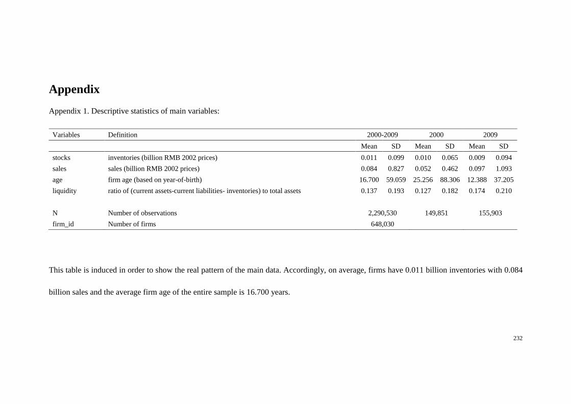
232
Appendix
Appendix 1. Descriptive statistics of main variables:
Variables Definition 2000-2009 2000 2009
Mean SD Mean SD Mean SD
stocks inventories (billion RMB 2002 prices) 0.011 0.099 0.010 0.065 0.009 0.094
sales sales (billion RMB 2002 prices) 0.084 0.827 0.052 0.462 0.097 1.093
age firm age (based on year-of-birth) 16.700 59.059 25.256 88.306 12.388 37.205
liquidity ratio of (current assets-current liabilities- inventories) to total assets 0.137 0.193 0.127 0.182 0.174 0.210
N Number of observations 2,290,530 149,851 155,903
firm_id Number of firms 648,030
This table is induced in order to show the real pattern of the main data. Accordingly, on average, firms have 0.011 billion inventories with 0.084
billion sales and the average firm age of the entire sample is 16.700 years.
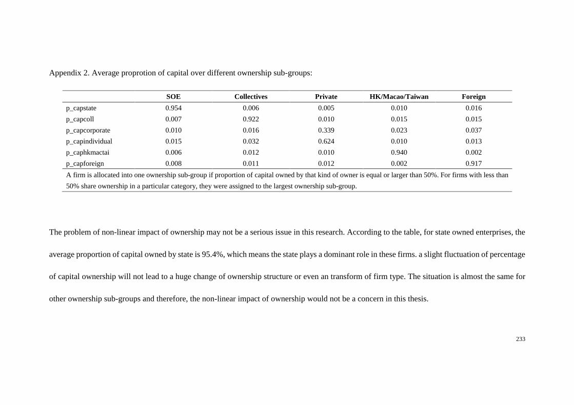
233
Appendix 2. Average proprotion of capital over different ownership sub-groups:
SOE Collectives Private HK/Macao/Taiwan Foreign
p_capstate 0.954 0.006 0.005 0.010 0.016
p_capcoll 0.007 0.922 0.010 0.015 0.015
p_capcorporate 0.010 0.016 0.339 0.023 0.037
p_capindividual 0.015 0.032 0.624 0.010 0.013
p_caphkmactai 0.006 0.012 0.010 0.940 0.002
p_capforeign 0.008 0.011 0.012 0.002 0.917
A firm is allocated into one ownership sub-group if proportion of capital owned by that kind of owner is equal or larger than 50%. For firms with less than
50% share ownership in a particular category, they were assigned to the largest ownership sub-group.
The problem of non-linear impact of ownership may not be a serious issue in this research. According to the table, for state owned enterprises, the
average proportion of capital owned by state is 95.4%, which means the state plays a dominant role in these firms. a slight fluctuation of percentage
of capital ownership will not lead to a huge change of ownership structure or even an transform of firm type. The situation is almost the same for
other ownership sub-groups and therefore, the non-linear impact of ownership would not be a concern in this thesis.

234
Appendix 3. Speed of adjustment:
The half-life convergence time is usually calculated based on a model in which the
dependent variable is specified as the difference between the observation in T and in
0:
ln𝐼𝑇,𝑖
𝐼0,𝑖= α + βln𝐼0,𝑖 + 휀𝑖
ln𝐼𝑇,𝑖 − 𝑙𝑛𝐼0,𝑖 = α + βln𝐼0,𝑖 + 휀𝑖
ln𝐼𝑇,𝑖 = α + (1 + β)ln𝐼0,𝑖 + 휀𝑖
where T is time period and β (assumed to be negative) can be used to measure the
actual speed-of-convergence.
b = −ln (1 + 𝛽)
𝑇
The half-life is ln(2)/b.
The model estimated here (an autoregressive distributed lag model) is different. Recall
that
𝐼𝑖𝑡 = 𝜑𝐼𝑖,𝑡−1 + 𝜋′𝑋𝑖𝑡 + 𝑣𝑖𝑡 (3.6)
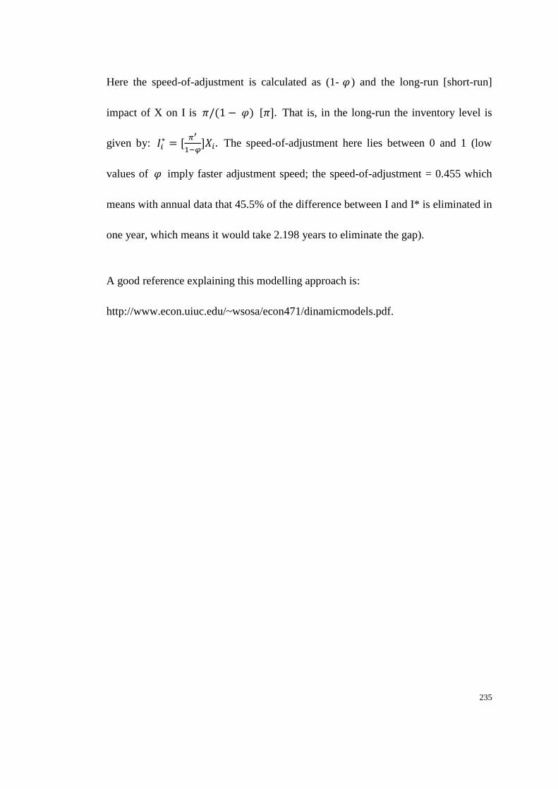
235
Here the speed-of-adjustment is calculated as (1- 𝜑 ) and the long-run [short-run]
impact of X on I is 𝜋/(1 − 𝜑) [𝜋]. That is, in the long-run the inventory level is
given by: 𝐼𝑖∗ = [
𝜋′
1−𝜑]𝑋𝑖. The speed-of-adjustment here lies between 0 and 1 (low
values of 𝜑 imply faster adjustment speed; the speed-of-adjustment = 0.455 which
means with annual data that 45.5% of the difference between I and I* is eliminated in
one year, which means it would take 2.198 years to eliminate the gap).
A good reference explaining this modelling approach is:
http://www.econ.uiuc.edu/~wsosa/econ471/dinamicmodels.pdf.