Embed Size (px)
Citation preview

Durham E-Theses
Premium Payback Period Model and its Application in
Stock Investment
XU, ZHILIN
How to cite:
XU, ZHILIN (2016) Premium Payback Period Model and its Application in Stock Investment, Durhamtheses, Durham University. Available at Durham E-Theses Online: http://etheses.dur.ac.uk/11813/
Use policy
The full-text may be used and/or reproduced, and given to third parties in any format or medium, without prior permission orcharge, for personal research or study, educational, or not-for-pro�t purposes provided that:
• a full bibliographic reference is made to the original source
• a link is made to the metadata record in Durham E-Theses
• the full-text is not changed in any way
The full-text must not be sold in any format or medium without the formal permission of the copyright holders.
Please consult the full Durham E-Theses policy for further details.
Academic Support O�ce, Durham University, University O�ce, Old Elvet, Durham DH1 3HPe-mail: [email protected] Tel: +44 0191 334 6107
http://etheses.dur.ac.uk

Premium Payback Period Model and its Application in
Stock Investment
By Zhilin XU
Supervisors: Dr Jing-Ming Kuo and Professor Richard Harris
A Dissertation Submitted for the Degree of
Doctorate in Business Administration
Durham University Business School
University of Durham
18th October 2016

i
Abstract
A simple and effective investment strategy has always been the pursuit of both
academicians and practitioners. This thesis introduces for the first time the concept of
Premium Payback Period (PPP), the time required to earn back the premium paid for
an asset. PPP is a powerful stock valuation model, which takes into account the
company’s current accounting information and future earning ability. In the stock
market, a stock’s PPP can be computed from its PB and ROE. In the real economy, a
company’s PPP can be observed from the date of establishment to IPO. As a rule of
thumb, stocks with PPP < 5 years are undervalued and stocks with PPP > 9.5 years are
overvalued, where the threshold PPP is obtained from observation in real economy.
PPP is proved to be an effective investment strategy in terms of stock selection as well
as market timing. A pilot empirical study in Chapter 2 shows that a portfolio of stocks
with PPP lower than 5 years can achieve excess return. In Chapter 3, I attempt to
demonstrate the power of PPP model in selecting undervalued stocks. The size effect
and PPP effect are incorporated in one framework and investigates both bull and bear
market conditions. Investment recommendation is to invest in firms with small size
and low PPP. When the indicators conflict, PPP criterion is the priority in the bear
market and size criterion is the priority in the bull market. In Chapter 4, I endeavor to
extend the application of PPP model to market timing. Both Treynor and Mazuy
Model and Henriksson and Merton Model confirm the poor market timing
performance of 10 Chinese equity-type funds. PPP model can help improve market
timing significantly by adjusting position in stock market in line with PPP value of
stock index. This research thus provides strong evidence that the PPP model performs
as an effective investment strategy by selecting undervalued stocks and entering or
exiting the stock market at appropriate timing.
Key Words:
Premium Payback Period, Stock Investment Strategy, Stock Selection, Market Timing

ii
Contents
Abstract ........................................................................................................................... i
Contents ......................................................................................................................... ii
List of Tables ................................................................................................................. v
List of Figures .............................................................................................................. vii
Declaration ................................................................................................................. viii
Statements of Copyright ............................................................................................... ix
Acknowledgments.......................................................................................................... x
Dedication .................................................................................................................... xii
Chapter 1 Introduction ................................................................................................... 1
1.1 Research Background ........................................................................................... 1
1.2 Relevant Literatures and Research Gap ............................................................... 9
1.3 Research Objective and Approach ..................................................................... 15
1.4 Significance of Research and Contributions ...................................................... 18
Chapter 2 Premium Payback Period Model: A New Method for Stock Valuation ..... 22
2.1 Introduction ........................................................................................................ 22
2.2 Literature Review ............................................................................................... 27
2.2.1 Discounted Cash Flow Models .................................................................... 28
2.2.2 Residual Income Model ............................................................................... 32
2.2.3 Relative Valuation Ratios ............................................................................ 37
2.2.4 PB-ROE Model............................................................................................ 42
2.3 Premium Payback Period Model ........................................................................ 45
2.3.1 Introduction to PPP Model .......................................................................... 45
2.3.2 Model Construction ..................................................................................... 47
2.3.3 PPP in Real Economy and Selection of the Critical Value ......................... 54
2.3.4 Comparison of PPP and Tobin’s Q.............................................................. 58
2.4 Practice of PPP Model and a Pilot Empirical Study .......................................... 60

iii
2.4.1 Data Collection ............................................................................................ 60
2.4.2 PPP Model in Fictitious Economy............................................................... 61
2.4.3 Determination of PPP Critical Value........................................................... 65
2.4.4 Practice of PPP Model for Investment Timing ............................................ 66
2.4.5 A Pilot Empirical Study of PPP ................................................................... 67
2.5 Conclusions ........................................................................................................ 78
Chapter 3 Practice of PPP in Stock Investment: A Perspective in Stock Selection .... 81
3.1 Introduction ........................................................................................................ 81
3.2 Literature Review ............................................................................................... 83
3.2.1 Size Effect.................................................................................................... 83
3.2.2 Value Effect ................................................................................................. 84
3.2.3 PPP Effect .................................................................................................... 85
3.3 Methodology of Empirical Study ....................................................................... 86
3.3.1 Determining a sample pool for investigation. ............................................. 86
3.3.2 Calculating PPP on a specific date .............................................................. 87
3.3.3 Classification of sample stocks in terms of size and PPP............................ 89
3.3.4 Computing daily returns for the categorized portfolios ............................... 90
3.3.5 Obtaining Jensen’s α for the portfolios ....................................................... 92
3.3.6 Evaluating the best performing portfolio and recommendations ................ 93
3.4 Size Effect and PPP Effect in Bear Market Conditions ..................................... 94
3.4.1 Data Selection and Description ................................................................... 94
3.4.2 Investment Portfolios based on 3x2 scenario of size and PPP .................... 96
3.4.3 Investment Portfolios based on 3x3 scenario of size and PPP .................. 102
3.5 Size Effect and PPP Effect in Bull Market Conditions .................................... 109
3.5.1 Data Selection and Description ................................................................. 109
3.5.2 Investment Portfolios based on 3x2 scenario of size and PPP .................. 111
3.5.3 Constructing Investment Portfolios based on 3x3 scenario of size and PPP
............................................................................................................................ 117
3.6 Conclusion ........................................................................................................ 123
Chapter 4 Practice of PPP in Stock Investment: A Perspective in Market Timing ... 127

iv
4.1 Introduction ...................................................................................................... 127
4.2 Literature Review ............................................................................................. 130
4.2.1 Market Timing Models .............................................................................. 131
4.2.2 Empirical Results for Fund Performance in China .................................... 136
4.3 Empirical Study of Investment Timing of Funds in China .............................. 140
4.3.1 The Development of Fund Market in China .............................................. 141
4.3.2 Model Construction ................................................................................... 144
4.3.3 Sample and Data Collection ...................................................................... 146
4.3.4 Empirical Results ....................................................................................... 151
4.3.5 Summary and Comments........................................................................... 156
4.4 PPP Model in Market Timing .......................................................................... 157
4.4.1 Practicing PPP on Individual Stocks ......................................................... 157
4.4.2 Derivation of PPP Model to Overall Stock Market ................................... 159
4.4.3 Practice of PPP for the Overall Stock Market ........................................... 161
4.4.4 An Empirical Test on Market Timing Ability of PPP Model.................... 169
4.5 Conclusion ........................................................................................................ 182
Chapter 5 Conclusions, Implications and Limitations ............................................... 185
5.1 Conclusions ...................................................................................................... 185
5.2 Implications ...................................................................................................... 189
5.3 Limitations ....................................................................................................... 190
References .................................................................................................................. 193

v
List of Tables
Table 1-1: Distribution of Individual Investors by Age as of 2015 ............................... 3
Table 1-2: Distribution of Individual Investors by Academic Background as of 2015 . 3
Table 2-1: Penman (1996)’s Exhibit of PB-PE Combinations ..................................... 41
Table 2- 2 Median ROE for Sample Stocks from 2005-2015 ...................................... 49
Table 2-3: Summary Statistics for PPP of 300 stocks .................................................. 72
Table 2-4: Summary of regression for portfolio composites ....................................... 74
Table 2-5: Comparison of Market Index and PPP Portfolio Returns ........................... 76
Table 3-1: Sample Numbers in 3x2 Scenario in Bear Market ..................................... 97
Table 3-2: Average PPP for Each Portfolio in 3x2 Scenario in Bear Market .............. 97
Table 3-3: Summary Statistics for Market and Portfolio Return in Bear Market ........ 98
Table 3-4: Regression Results of 6 Portfolios in 3x2 Scenario in Bear Market .......... 99
Table 3-5: Jensen alpha for Size-PPP portfolios in Bear Market ............................... 100
Table 3-6: Sample Numbers in 3x3 Scenario in Bear Market ................................... 102
Table 3-7: Average PPP for Each Portfolio in 3x3 Scenario in Bear Market ............ 103
Table 3-8: Summary Statistics for Market and Portfolio Return in Bear Market ...... 104
Table 3-9: Regression Results of 9 Portfolios in 3x3 Scenario in Bear Market ........ 105
Table 3-10: Jensen alpha for Size-PPP portfolios in Bear Market ............................. 106
Table 3-11: Sample Numbers in 3x2 Scenario in Bull Market .................................. 111
Table 3-12: Average PPP for Each Portfolio in 3x2 Scenario in Bull Market ........... 112
Table 3-13: Summary statistics for market and portfolio returns in Bull Market ...... 113
Table 3-14: Regression Results of 6 Portfolios in 3x2 Scenario in Bull Market ....... 114
Table 3-15: Jensen alpha for size-PPP portfolios in Bull Market .............................. 115
Table 3-16: Sample Numbers in 3x3 Scenario in Bull Market .................................. 117
Table 3-17: Average PPP for Each Portfolio in 3x3 Scenario in Bull Market ........... 118
Table 3-18: Summary Statistics for Market and Portfolio Return in Bull Market ..... 118
Table 3-19: Regression Results of 9 Portfolios in 3x3 Scenario in Bull Market ....... 120

vi
Table 3-20: Jensen alpha for Size-PPP portfolios in Bull Market ............................. 121
Table 4-1: Composition of China’s Fund Market by 2013 ........................................ 144
Table 4-2: Definition of Sub-samples ........................................................................ 148
Table 4-3: Ten Sample Funds Selected for Empirical Study ..................................... 150
Table 4-4: Empirical Result of China’s Fund Performance ....................................... 152
Table 4-5: Empirical Results for Sub-period Samples ............................................... 153
Table 4-6: Summary of Stock Selectivity and Market Timing of China’s Fund ........ 155
Table 4-7: Definition of Various PPP Types .............................................................. 161
Table 4-8: Different Critical Values for PPP .............................................................. 163
Table 4-9: Case Study of PPP in China’s Stock Market ............................................ 167
Table 4-10: Regression Results of TM and HM models ............................................ 174
Table 4-11: Comparison between Original Fund and Adjusted Investment .............. 175
Table 4-12: Market Timing Effect of Buy-and-Hold Strategy ................................... 177
Table 4-13: Market Timing Effect of PPP Strategy ................................................... 179
Table 4-14: Summary of Test for Individual Stocks .................................................. 180
Table 4-15: Cumulative Returns of Buy and Hold vs PPP Timing ............................ 181

vii
List of Figures
Figure 1-1: Most Widely Used Valuation Methods ..................................................... 11
Figure 2-1: Tobin’s Q in China’s Stock Market ........................................................... 63
Figure 2-2: Premium Payback Period in China’s Stock Market .................................. 64
Figure 2-3: PB-ROE of Shanghai-Shenzhen Composite 300 stocks ........................... 68
Figure 2-4: Percentage of stable and unstable dividend policies in China .................. 71
Figure 2-5: Cumulative returns for market index and PPP portfolio ........................... 77
Figure 4-1: Development of China’s Fund Market in Quantity and NAV ................. 143
Figure 4-2: Shanghai Security Composite Index from 2007 to 2013 ........................ 148
Figure 4-3: SSCI and PPP in China’s Stock Market .................................................. 163
Figure 4-4: Market Timing and Cumulative Return .................................................. 170

viii
Declaration
No part of this thesis has been submitted elsewhere for any other degree
or qualification in this or any other university. It is all my own work
unless referenced to the contrary in the text.

ix
Statements of Copyright
The copyright of this thesis rests with the author. No quotation from it
should be published without the author's prior written consent and
information derived from it should be acknowledged.

x
Acknowledgments
After all these years of hard work, it is necessary to express my gratitude to those
people who have been helping and supporting me during my pursuit for Doctorate in
Business Administration from Durham University.
My first thanks go to my principal supervisor, Dr Jing-Ming Kuo, whose patience,
guidance and encouragement throughout my doctoral study, enabled me to develop an
understanding of what DBA is and what is indeed the purpose behind a thesis.
Discussion with him is always enlightening and fruitful despite the great time
difference between UK and China. Without his helpful advice and valuable comments,
my DBA journey would not have been the same.
Second, I would like to thank Ms Ning Pan to introduce the great DBA programme
from Durham University to Fudan University. Without her contribution, I would not
have the opportunity to get access to world’s elite minds and ideas in Shanghai. I am
also deeply indebted to her for persuading me to join the programme.
Most of all, I am sincerely grateful to my wife and my three daughters for their
encouragement, commitment and love, which is indispensible for me to complete this
part time research programme.

xi
To everyone else who is not mentioned here but contributed to my DBA directly or
indirectly, I thank you all.

xii
Dedication
To my beloved wife and three daughters.

xiii

1
Chapter 1 Introduction
Every day, millions of stock investors, no matter individual or institutional, have to
face a common but often perplexing question: is the stock worth investing now?
Finding the intrinsic value of a stock is always an endless effort for investors.
However, despite the advancement in computation models and improvement in
market environment, still no one can answer the above question with full confidence.
1.1 Research Background
The optimal investment strategy in the financial market, inter alia stock market, has
consumed the wisdom of several generations of financial theorists and practitioners.
The existence of such a strategy is a conundrum in itself. The milestone Efficient
Market Hypothesis (EMH) proposed in a seminal paper by Eugene Fama (1970),
ruled out such possibilities. However, efficient market is valid only under very
rigorous conditions, one of which is investor’s rationality. In a well functioning stock
market with rational investors, it is impossible to yield excessive return and the
discussion in this field comes to deadlock. Obviously these presumptions are far away
from reality and it is widely noted on the investor’s irrational behaviour and relevant
market anomalies.
One possible but not exclusive cause of investor irrationality is the lack of education
and training. But even those financial elites with MBA or PhD degrees in finance are
still vulnerable to madness and emotions. Again and again, it is discovered that

2
educational level plays a negligible part in irrational behaviour, e.g. herding behaviour.
In the book of Investment Madness (Nofsinger, 2001), such emotions are
systematically summarized, and disposition effect is among the most significant
phenomena. The disposition effect takes its root in the human psychology of seeking
pride and avoiding regret. Such is human nature that investors are bounded to various
personal limitations and their investment decisions are very likely to deviate from
optimum.
According to Standards for Classification of Stock Investors issued by China
Securities Regulatory Commission (CSRC), stock investors can be classified as
individuals, institutions and corporations. Institutional investors mainly refer to funds,
security companies, insurance companies, trust companies, QFII, social security fund,
etc. Corporation shareholders refer to the business entities other than institutional
investors. Corporation shareholders are usually original shareholders or strategic
investors before IPO or by means of directed additional issuance or acquisition.
Usually corporation shareholders trade infrequently despite the large proportion of
market value they hold. According to the Shanghai Stock Exchange Statistics Annual
2016, individuals, institutions and corporations held respectively 25%, 15% and 60%
of total market value. The three classes of investors contributed to 86.91%, 10.47%
and 2.06% of the trading volume in the year of 2015. In conclusion, individual
investors are an important active player in China’s stock market.
It is acceptable that individual investors are irrational because of their lack of

3
expertise and experience as well as the so-called human weakness. Surprisingly,
however, such irrationality is also prevalent among experienced and mature investors,
best represented by investment managers in the institutions.
The major difference between normal individual investors and institutional investors
is the latter’s specialized knowledge and access to in-depth information and resources.
According to China Securities Depository and Clearing Corporation Limited, the
majority (69.11%) of Chinese individual investors are under the age of 40 years by the
end of 2016, and only a small proportion (25.3%) of the individual investors have a
bachelor’s degree or above.
Table 1-1: Distribution of Individual Investors by Age as of 2015
Age Under 30 30-40 40-50 50-60 Up 60
Percentage 37.64% 31.47% 19.05% 7.79% 4.06%
Data Source: China Securities Depository and Clearing Corporation Limited (CSDC)
Table 1-2: Distribution of Individual Investors by Academic Background as of 2015
Academic Under Middle
Education
Middle
Education
Higher
Education Bachelor
Master or
above
Percentage 23.59% 24.24% 26.87% 21.47% 3.83%
Data Source: China Securities Depository and Clearing Corporation Limited (CSDC)
On the contrary, people who are in charge institutional investors have more
investment experience and better educational background. The best examples of these
people are the managers of the public offered funds. According to the survey released
by China Business Press Release Newswire in January 2014, the average age of the

4
fund managers is 38.2 years old. Out of the fund managers, 81.15% have a master
degree, 13.66% have doctoral degree, 4.92% have a bachelor degree, and more than
50% of them graduate from China’s top 4 universities. In addition, 72% are Chartered
Financial Analyst (CFA), 15% have certification of Financial Risk Management
(FRM) and 15% are Certified Public Accountant (CPA) in China. Besides the personal
experiences and qualifications, fund managers have another dominant advantage over
the individual investors. They have a strong research team who can provide
intellectual support in macroeconomic analysis, industrial analysis, company-level
analysis, etc. Another advantage of fund managers is that they are in charge of much
more capital than individual investors so they are more able to diversify the allocation
of capital and reduce systematic risks.
From observations in China’s stock market in the past few years, it is found that even
some fund managers enter in bull market (up to 6000 points) and exit in bear market
(down to 1600). This phenomenon is somewhat inexplicable in the sense that fund
managers or institutional investors are rational compared with individual investors.
Institutional investors, including some security companies, are supposed to formulate
decisions based on scientific forecast. However, it has been repeatedly tested that their
forecast is often incorrect. Ostensibly, the security companies make predictions after a
fundamental analysis of the economy, however, as one of the practitioners, I can
reveal that a considerable proportion of the prediction is based on the status quo and
trend on the prediction date, therefore the forecast is poorly grounded.

5
According to an investigation on Researcher Forecast Accuracy in China’s Security
Companies in 2009 conducted by Investor China (Issue 11, 12 March, 2010), more
than half of the researcher recommendations are proved to be unsuccessful. The
investigation covers 21,300 reports written by 1,042 researchers from 42 China’s
security companies from 1 July 2008 to 30 June 2009 and compares the recommended
securities with the market index. It is astonishing to find that only 47% of the
researchers are able to provide relatively accurate recommendations. More
sarcastically, the bigger the brand of the security company is, the poorer its
recommendation is, with China International Capital Corporation Limited (China’s
top investment bank) ranking lowest.
The change in position of stock represents a specific investment strategy. If the
change in stock position is in advance of the changes in the stock index, such
investment strategy is successful. To be more specific, if one investor increases stock
position at time t and the market index rises at t+1, such a change in position brings
profit. If one investor decreases stock position at time t and the market index drops at
t+1, such a change in position avoids loss. If the position changes is opposite of the
market index, such investment is a failure. Observations from the second half of the
year 2009 identify a decline in positions of two types of funds: Open-end Fund (from
86.36% to 81.38%) and Close-end Fund (from 76.55% to 72.67%) during the third
quarter of 2009 (Hu and Gao, 2009). However, the market index turned out to witness
a growth from 2779.47 to 3039.86 in the fourth quarter. The negative correlation
between fund’s stock position and market index serves as evidence that fund
6
managers and institutional investors are not smart during the chosen period.
In such a stock market with both irrational individual and institutional investors, there
must be full of opportunities for excess returns. Specifically, considering that China’
stock market is still immature, traditional financial theories almost fail. China’s stock
market has two significant characteristics which set apart from mature markets, where
the tradition financial theories are developed. A fundamental of a company cannot be
reflected in the price of its stock.
The first characteristic is that state-owned enterprises (SOEs) play an important role
in China’s stock market. SOEs account for 35% of China’s A-share listed company in
terms of number and 48% in terms of market value as of 2015. On one hand, SOEs
which have a very complicated decision making process, have relatively low
operational efficiency and thus poor performance. On the other, SOEs have a good
control of resources, specifically in industries with limited competition. These two
aspects inter-link with each other. Despite the low efficiency and poor performance,
SOEs are able to reshape its fundamental by restructure, merger & acquisition, or
change of business scope, resulting in the considerable change in its stock price.
Therefore, investors have to pay more attention to the “information” than the
fundamental factors of the company.
The other characteristic of China’s stock market is its sensitive to policies, e.g.
macroeconomic policy, monetary policy, IPO policy, etc. It also occurs in other
markets. The difference is that when the stock market is in an abnormal condition,

7
Chinese investors expect for a special policy and the regulator’s action reinforces the
investors’ expectation. After hitting a historical high of 1558 points in February 1993,
the Shanghai Security Composite Index (SSCI) slumped to 333 points in July 1994.
The index was almost 80% off within one and half years. The market was expecting a
so-called “save-the-market” policy. As expected, on 30 July 1994 China Securities
Regulatory Commission (CSRC) put into effect three major policies to stabilize the
stock market: (1) provisional suspension of IPO, (2) strict control of right offering for
listed companies, (3) expansion of allowed capital for stock investment. Market
intervention has also occurred later in different market conditions and indeed exerted
an influential impact on the stock market. More interestingly, China’s stock market is
easily affected by editorials in People’ Daily.
Based on the above discussions, investors do not have to care about the fundamentals
of the companies. What really concerns is an easier access to the policy or information
from the government, which can produce considerable speculative return rather than
investment return.
Shanghai Securities Composite index has experienced rollercoaster-style movement in
the past 10 years and is still very volatile recently in the aftermath of global financial
crisis and gloomy domestic economic expectation. The deviation of the stock price
and stock index from their fundamental as a result of irrational investors makes it
possible for genius investors to identify undervalued stocks. The correct prediction on
the index is also crucial to a successful investment strategy.

8
There are two major schools of investment philosophy, namely value investment and
technical investment. Both investors believe in the imperfection of stock market so
that they have the potential to beat the market and achieve excess return after doing
their own homework. This is also the basic premise for this thesis otherwise all
arguments are in vain. A value investor determines the intrinsic value of a stock by
looking at the strength of the business, its financial status and the operating
environment including macroeconomic factors. A value investor sticks to the firm
belief that efficient market hypothesis works in the long term so that his endevours to
seek for undervalued stocks will finally pay off in the future. Technical investors
argue that fundamental elements of the stocks have already been completely priced. In
the short run, the driving force to pull stock price away from fundamental level is the
psychological aspect or the trading behaviour of the investors, which is exhibited
from past movements of the stock price. Technical investors attempt to predict future
movement from the observation of past movements. Technicians are usually more
short-term traders by nature, contrasting with the long-term view fundamentalists
generally take. Yet even experienced investors cannot reach consensus on which type
of analysis can generate higher returns.
More scholarly speaking, value investment seems to have a more theoretical ground
than technical investment. Therefore, a well-educated investor tends to apply the
value investment; however the fact is that in many cases technical analysis does
provide better return, especially in the short run. Both academicians and practitioners
endeavor to find better investment strategies.

9
1.2 Relevant Literatures and Research Gap
Generally speaking, there are two schools of stock valuation models, i.e. absolute
valuation models and relative valuation models. Absolute valuation is targeted at the
intrinsic value of one stock by analyzing its fundamentals and estimating its future
financial performance. Relative valuation, in contrast, examines the value of a stock
by comparing with its competitors.
Absolute valuation models attempt to determine a stock’s intrinsic worth based on its
projected cash flows. The most well-known absolute valuations models are Discount
Dividend Model (DDM) and Discount Cash Flow Model (DCF). DDM was first
proposed by William (1938), viewing that the value of a stock is equivalent to the
present value of all future dividends. DDM has several variants in terms of different
assumptions of dividend payments, e.g. zero-growth model and constant growth
model (Gordon, 1962). The three stage growth model (Molodovsky et al, 1965) takes
into account different dividend growth rates for a more accurate estimation. The
limitation of DDM is the assumption of a stable or predictable dividend payment
policy. In reality, few companies pay out dividends in the manner defined in existent
models.
DDM implies that dividend is the only yield for shareholders. DCF relaxes the
assumption and emphasizes on the free cash flow available. DCF is a model with
solid theoretical foundation because it incorporates all future cash flows related to the
company. The free cash flow can either be free cash flow to the firm (FCFF) or free

10
cash flow to the equity (FCFE), discounted on correspondent rate. DCF model also
requires analysts to have a clear understanding of the company’s future financial
performance. Predicting future cash flow is relatively easier for companies in a stable
stage than fast growing companies.
Both DDM and DCF models neglect two important issues. The first one is that these
two models neglect the cost of equity capital, in another word, opportunity cost for
investors. The other one is that these two models neglect the current accounting
information e.g. book value of equity. Edward and Bell (1961) proposed the first
generation of Residual Income Model (hereafter RIM) to solve the problems. Residual
income is the income generated by a firm after accounting for the cost of equity
capital. Residual income is an economic income rather than an accounting income. A
firm’s value can thus expressed as the sum of its equity’s book value and discounted
future residual income. Different treatments of residual income lead to different
specifications of RIM, e.g. Economic Value Added (EVA) model (Steward, 1991),
Ohlson Model (Ohlson, 1995) and Feltham-Ohlson model (Feltham and Ohlson,
1995), etc. Feltham-Ohlson model is one of the milestones in valuation models.
Feltham-Ohlson model perceives a company’s value as the aggregate of its book value
of equity and future profitability, highlighting the importance of accounting
information in valuation. Bernard (1995) declares that Feltham-Ohlson model is
“getting off to the right start” and his empirical study shows that valuation by
Feltham-Ohlson model can explain 0.68-0.8 of stock price but traditional DCF models
can only explain for 0.29. Penman and Sougiannis (1998) compared DDM, DCF and

11
Feltham-Ohlson models using data from 1973 to 1992, finding that Feltham-Ohlson
model is superior to the other two.
Although absolute valuations models, which are based on the future cash flow or
economic profit, have a logical grounding, they are not frequently used in investment
practice due to the difficulty in precise prediction of future. It would require
tremendous amount of financial information for a reliable forecast and the result is
dependent on analysts’ subjective selection of model parameters including cash flows
and discount rate. The Morgan Stanley’s survey entitled “How We Value Stocks” was
published in 1999. The survey investigated the valuation methods most widely used
by Morgan Stanley Dean Witter's analysts for valuing European companies.
Surprisingly, fewer than 20% analysts use DCF model, which only ranks fifth, behind
multiples such as PE Ratio, EV/EBITDA and EV/EG.
Figure 1-1: Most Widely Used Valuation Methods
Source: Morgan Stanley Dean Witter Research
Note: Weighted by the market capitalization of the industry in which it is applied.

12
The percentage falls below 15% in China according to China’s WIND Data. The
majority of security analysts prefer the other school of valuation, i.e. relative
valuation, also called valuation using multiples. It refers to the notion of comparing
the price of a stock to the market value of similar asset. Absolute valuation can judge
whether a stock is worth investing or not, whereas relative valuation can justify which
stock is a better target.
Relative valuation employs a series of ratios for a group of similar stocks and the
stock with a below average ratio is deemed to be undervalued and worth investing.
The most commonly adopted multiples fall into two categories, respectively based on
market value and firm value. Market value based multiples include price to earnings
(PE), price to book value (PB), price to sale (PS), price to cash flow (PCF). Firm
value based multiples include EV/EBITDA, EV/sales and Tobin’s Q (Tobin, 1969).
Generally speaking, a lower ratio is "better" (cheaper) and a higher ratio is "worse"
(more expensive). Basu (1977) found it true for PE and Senchack and Martin (1987)
proved the case for PS.
Different ratios observe firm value from different perspectives and have their specific
limitations. Earning in PE ratio is an accounting element which can be controlled by
managers using a accounting policy at their advantage. Book value in PB ratio is the
original price of asset minus depreciation and amortization, but it does not account for
inflation and technological progress. PS ratio does not take into consideration of
profitability whereas EV/EBITDA does not take into consideration of growth.

13
Sometimes two ratios have contradicting indications for valuation. Therefore it is
recommended to use at least 2 ratios to leave less room for errors. For instance, the
PEG ratio (price/earnings to growth ratio) first introduced by Frina (1969) and later
popularized by Peter Lynch (1989) is a valuation metric for determining the relative
trade-off between the price of a stock, the earnings generated per share (EPS), and the
company's expected growth. Lynch proposes that a fairly valued company will have
its PEG equal to 1. Stock with PEG <1 is undervalued and PEG>1 is overvalued.
Wilcox (1984) brought forward a framework which incorporates PB and ROE and
proved the linear relationship between log (PB) and ROE. If the actual PB is higher
(lower) than the one indicated by the linear relationship, the stock is overvalued
(undervalued).
Tobin’s Q model provides a new horizon to valuation. Tobin’s Q is the ratio between a
physical asset's market value (numerator) and its replacement cost (denominator). If
the market value reflected solely the recorded assets of a company, Tobin's Q should
be 1. If Tobin’s Q is larger than 1, the market value is greater than the value of the
company's recorded assets, so that investors are encouraged to invest in physical
assets rather than buy the stock. If Tobin’s Q is smaller than 1, the asset is
undervalued in the stock market than in the real economy. Therefore, the ratio serves
as the nexus between financial markets and markets for goods and services. Another
application for Tobin’s Q is to determine the valuation of the whole market in ratio to
the aggregate corporate assets. Tobin’s Q model has two shortcomings. The first one

14
is that it only addresses the physical asset and does not include intangible asset such
as technology know-how and human capital. The second one is that the replacement
cost, which is a lagging and inaccurate measure is too difficult to estimate because it
is influenced by many factors. Different economic environments, for instance high
inflation, will skew the metric substantially.
Stock valuation is a complex process and it is quite impossible that one single model
can solve all the problems. Every model has its own advantages and disadvantages.
DCF models have a strong theoretical grounding and simple expression, but future
cash flows are not readily available and the models do not take into consideration of
current accounting information. The determination of future cash flow and discount
rate is subject to the analyst’s experience and preference, which can lead to totally
different results. So the application of DCF models in practice is not often. On the
other hand, the multiples in the relative valuation models are very easy to obtain but
each multiple is only applicable for a particular group of stocks and is vulnerable to
external factors. The crosscheck by more than two multiples may help reduce the
chance of misjudgment, but in some occasions, two relative ratios contradict each
other. Even the Noble Prize winner Tobin’s Q theory has many flaws despite its
perfect economic interpretation. In conclusion, there is plenty of room for
improvement in the valuation models. This research endeavors to provide a new
valuation model which share the advantages of existent models and eliminate the
disadvantages with my best effort.

15
1.3 Research Objective and Approach
The objective of this research is to present one of my own investment strategies which
have been practiced for more than a decade. The full name of the model is called
“Premium Payback Period” model (hereafter PPP model), which literally means the
model to compute the required period to claim back the premium paid for an asset.
The premium refers to the gap between price and book value. The comparison
between the model-based data and the benchmark indicates whether the stock is
overvalued or undervalued. PPP model also takes a value investment perspective. In
this thesis, I attempt to show that PPP model is not only a good theory but also a
powerful tool in investment practice. More importantly, the effective result of PPP
model can indicate that value investment is viable in China’s stock market. An
investment strategy involves two dimensions. The first one is identification of stocks
worth investing, i.e. stock selection. The second one, also equally important is to
decide when to buy and when to sell, i.e. market timing. I also attempt to demonstrate
PPP model’s capacity in both dimensions.
To achieve the research objectives stated above, four other chapters are arranged to
fully discuss the relevant topics. In Chapter 2, I will present PPP model and explain
how it is constructed and I will also show how to apply PPP model in investment
practice. In Chapter 3, I attempt to show how to apply PPP in selection of stocks
under different market conditions and test whether the stocks selected can generate
excess return. In Chapter 4, I will extend the application of PPP model in another

16
dimension, market timing and show that PPP model can improve investor’s ability in
market timing. Chapter 5 is the conclusion of this thesis. The details of the following
four chapters are arranged as below.
In Chapter 2 “Premium Payback Period Model: A new method for stock valuation”, I
show how PPP model is constructed and the mathematical and economic indication of
the model. PPP model belongs to the family of value investment which is based on the
stock valuation. Tradition views are that the stock value is solely dependent on its
future cash flow but more and more researchers point out that the current accounting
information is equally important. In Chapter 2, I attempt to develop a framework to
count for both current book value of asset and future earning ability in determining
stock value. The concept of premium payback period is proposed to measure how
long it takes the premium paid in purchasing stocks to be rewarded by company
earnings. Stocks with low PPPs are safer and profitable investment. In this chapter, I
also provide an easy method to calculate PPP in stock investment and how to
determine the benchmark criteria for PPP index. The benchmark is obtained from
observation in real market by the measure of time required for a firm from
establishment to IPO in Growth Enterprise Market Board. A pilot empirical study is
then conducted, indicating that normally stocks with PPP shorter than 5 years can be
viewed as value stocks and can generate excess return.
In Chapter 3 “Practice of PPP in Stock Investment: A Perspective in Stock Selection”,
I demonstrate the PPP model’s ability to identify undervalued stocks in an effort to

17
achieve excess return. A stock’s excess return is its actual return over what can be
justified by Capital Asset Pricing Model. Excess return is not only a practical issue
but also of theoretical interest. In this Chapter, excess return is explained and achieved
by means of size effect and PPP effect. Size effect refers to the fact that small size
stocks generate higher returns than large size stocks. PPP effect refers to the fact that
stocks with low PPP can generate higher return than those with high PPP. Both size
effect and PPP effect are proved to be influential to stock returns, and one effect may
be more influential than the other in different market conditions. A sample bear
market and a sample bull market are both investigated respectively, demonstrating
how the application of PPP method combined with size selection method can help
pick stocks and construct well performing portfolios. Investment recommendations
are provided for the two market conditions. Generally speaking, it is recommended to
buy stocks with small capitalization and low PPP and sell stocks with large
capitalization and high PPP. In bear market, PPP effect is more dominant whereas in
bull market size effect is more dominant.
In Chapter 4 “Practice of PPP in Stock Investment: A Perspective in Market Timing”,
I demonstrate the PPP model’s ability to identify investment opportunities, i.e. when
to buy and when to sell. Excess return for an equity investment portfolio depends on
the investor’s decision of stock selection and market timing. Fund managers are
supposed to have both stock selectivity and market timing abilities because of their
expertise and experience. However, empirical studies in China as well as in foreign
countries exhibit no convincing evidence that fund managers have either of these

18
abilities. In this chapter, I will adopt the traditional Trenyor and Mazuy Model (TM
model) as well as Henriksson and Merton Model (HM model) to investigate the
period from 2007 to 2013 using weekly data. The empirical result shows no
significant market timing ability and in some certain period even negative market
timing. Premium Payback Period Model, which is developed for valuation of
individual stocks, is adjusted for the overall market to assess whether the overall stock
market is overvalued or undervalued. The application of PPP for the overall stock
market is demonstrated by case study across China’s stock market history. PPP is
found to be effective in predicting market trend and is proved to be good investment
tool for market timing. The introduction of PPP can assist in adjusting the stock
position of investment and exhibit better market timing ability for both funds and
individual stocks.
In Chapter 5, I will draw the conclusions that PPP model excels in stock selection as
well as market timing and provides the inherit logic behind the model. Then this
chapter delivers a clear and systematic summary on how to employ PPP in stock
investment for practical guidance. Despite the excellent performance of PPP model in
stock selection and market timing, I also point out the underlying limitations of the
model, the presumption of stable ROE and the negligence of investors’ psychology,
which can be explored by further research to improve PPP model.
1.4 Significance of Research and Contributions
This research is contributive in both theory and practice.

19
First and foremost, this research proposes a new model and criterion, named
“Premium Payback Period” for stock investment. PPP model is such a model that
takes into accounts both current accounting information and future earnings, that has a
solid theoretical grounding and easy application, that can evaluate a single stock as
well as the entire market. The analytical framework of PPP includes the two important
elements of investment concern, price to book value (PB) and return on equity (ROE).
Although this research is not the first attempt to combine PB and ROE in a single
framework, it does attempt to provide a unified analysis of PB and ROE to generate a
single indicator for investment guidance. The argument that stocks with lower PPP
values are more favorable to those with higher PPP values unveils a potential
connection between real economy and fictitious economy. Such a nexus has been
addressed in the Tobin’s Q theory, but Tobin’s Q theory only analyses it in a static
manner. PPP model employs a dynamic view on how real economy and fictitious
economy is linked. This research also perceives the time duration from a company’s
establishment to initial public offering in Growth Enterprise Market (GEM) of
China’s stock market or Second-board Market in other countries as the benchmark
PPP in the real economy. A stock with a lower PPP than the benchmark is undervalued
and is worth investing. This is how PPP model serves as a bridge between real
economy and fictitious economy.
As a DBA thesis, practical value is equally important and desirable. The most direct
impact of this research is to conclude an investment strategy on what to invest and
when to invest. The question of what to investment is no longer a big problem. The

20
classic portfolio theory and risk diversification have offered guidelines for stock
selection and capital allocation. But the theories remain well-structured theories and
perform poorly in real practice. In this research PPP model is proved to a good
investment strategy with numerous advantages. First of all, it is easy to apply by
merely retrieving basis financial data of the company and conducting easy calculation.
Second, unlike technical analysis, the PPP strategy has a solid theoretical foundation.
Thirdly, PPP can be used both in absolute valuation and relative valuation, by
comparing it with the PPP in the real economy or with PPP values of other stocks.
Finally and equally importantly, unlike other value investment strategies, PPP model
can be used to select undervalued stocks as well as to indentify investment timing.
It is widely recognized that when to invest has been pestering both individual and
institutional investors. Disposition effect refers to the selling of winners and buying of
losers. As far as timing is concerned, the disposition effect also applies to holding
losers too long and selling winners too soon. Holding losers too long indicates that the
stocks with dropping price will continue its poor performance and will not rebound as
much as wished; selling a winner too soon implies that it would have continued its
favorable momentum if the selling is postponed. PPP model is meant to pinpoint the
exact timing for buy and sell, or in other words enter or exit the stock market. The
solution of timing problem will definitely increase investment performance and
efficiency.
In conclusion, this study contributes both to theory and practice with the new model

21
of PPP. It inherits the new advancement in valuation by means of current accounting
information and future earning ability and provides a unified way to evaluate both
individual stocks and the entire stock market. The advantages of PPP model are its
easy application, solid theoretical logic, linkage between real and fictitious economy
as well as its application in both stock selection and market timing. Last but not least,
the above contributions are based on the author’s willingness and effort to make
public the investment strategy which would otherwise be merely an investment secret.

22
Chapter 2 Premium Payback Period Model: A New Method for Stock Valuation
2.1 Introduction
Chinese stock market was reactivated in December 1990 and since then the total value
of Shanghai and Shenzhen stock markets have grown rapidly to over 10 trillion USD
in June 2015, almost equal to China’s GDP in the previous year. The development of
Chinese stock market is strengthened by the participation of first mutual fund in 1997.
Since then the Chinese stock market should have been more mature and stable.
Unfortunately, the market behavior is not significantly different from before when
there were only individual investors in the market. The dynamics of the stock market
in China has been equally volatile and unpredictable. After several years of bear
market till 2006, China’s stock market bounced from 998 to 2245 points. The
Shanghais Security Composite Index even reached a historical peak above 6000 in
2007. Many professional investors were taken aback by the extreme bull market,
attracting more new investors to enter the market. As a result the number of active
stock account hit 100 million in 2007. To the investors’ great disappointment, the bull
market does not exist for long and soon the stock index dived to half of the peak
around 3000 points. Many investors have entered the stock market when the index
was above 5000, concluding from the recent trend and believing that the stock market
can provide easy money. The unsuccessful investment is resulted from the
overconfidence of technical analysis and trend investment. The recent turmoil in

23
China’s stock market again reshuffles investors’ opinion about it. It took a few months
for the index to rise from below 3000 points to over 5000 points and it took even
fewer weeks for the index to fall dramatically from above 5000 points to below 3000
points.
It is common knowledge that when the stock price goes too high above its intrinsic
value, it is doomed to go down. However, these irrational investors turn blind to the
common relative valuation indicators such as PE and PB and only believe that the
market can rise as long as possible. Therefore it is necessary to restate the concept of
value investment for three reasons.
Firstly, China’s stock market enters a new stage and entails value investment which is
a mature idea and has been practiced for decades in foreign stock markets. This idea
attracted investors’ attention in 2003 when outdated investment ideas were heavily
criticized. At the initial stage of China’s stock market from 1992 to 1997, the
movement of stock price was irrelevant to fundamental factors and speculation was
universal. Such conditions changed afterwards with more institutional investors and
experienced individual investors. The completion of share structure reform exerted a
powerful influence on the stock market and neglecting fundamental factors could be
disastrous.
Secondly, on the demand side, Chinese stock investors are learning to be more
rational and value investment is more welcome. After Chinese stock investors
experienced the huge upside movement in 2007 and huge downside movement in

24
2008, they started to reflect on their investment philosophies and value investment
was reinforced. Even if the lesson is not serious enough, the recent movement of stock
index like a rollercoaster reminds investors of value investment. Still many other
investors doubt the validity of value investment in China and argue that value
investment is air in the attic for China’s stock market and the investment environment
is not suitable for value investment. To test the suitability of value investment in
China is urgent and is one of the research aims.
Value investment was first brought forward by Benjamin Graham and David Dodd
(1934) in their masterpiece Security Analysis. They advocate that investors pay more
attention to the value of companies per se than the fluctuations of stock market. This
old and simple philosophy is enriched and practiced by Glenn Greenberg, Warren
Buffett, Peter Lynch among others and leads to considerable investment reward.
The idea of value investment is merely to compare intrinsic value and market price of
stocks, so simple that not many investors take it seriously. Value investment is
founded on two basic presumptions: (1) market price always deviates from intrinsic
value, and (2) market price always tends to revert to intrinsic value. The discrepancy
between stock value and price consists as an investment risk. Value investors buy
stocks whose prices are sufficiently below their values. The gap is the so-called
margin of safety, an important concept for value investment. The greater a stock price
deviates below the intrinsic value, the safer the investment is.

25
Value investors are extreme risk averters, who buy stocks as cautiously as if they buy
out the whole company. Margin of safety is their weapon to fight against risks due to
limited investment ability, stock market fluctuation and company development
uncertainty. Margin of safety can help to buffer investor’s loss against these adverse
factors.
Margin of safety makes profitable investment possible, which sets itself apart from
modern investment theories. First and foremost, value investment disagrees Market
Efficiency Hypothesis and argues that the phenomenon of unmatched stock price and
value is normal and key to the success of value investment. According to modern
finance theories, return is positively related to risk; in contrast, value investment
advocates that high return can always be accompanied by low risk, because of margin
of safety.
Value investment emphasizes the intrinsic value of an asset and attempts to compare it
with its price. If the price is lower than the intrinsic value, it is worth to buy, otherwise
the stock is regarded as overvalued and not worth to buy. Both theorists and
practitioners have developed many valuation methods to decide the intrinsic value of
the stock so that the value and the price are comparable in one framework. The
intrinsic value of a stock is dependent on a series of factors including macro economy,
industrial cycles and company-specific elements. Value investors pay great attention
to the margin of safety. When the price of a value investment product goes too high, it
is no longer safe and loses its value. The perception of margin of safety is quite

26
different from momentum investment. When the price continues to climb, the margin
of safety is undermined and investment is not recommended. However, momentum
traders believe with no concrete economic ground that the trend is sustainable. A
rational investor should be a value investor. De Bondt and Thaler (1985) investigated
the monthly cumulated excess return and proposed the over-reaction hypothesis,
concluding that the average return of losers portfolio (value stocks) is 19.6% higher
than market return while the average return of winners portfolio is 5% lower than
market return.
How safe is a stock investment? To what extent is the stock price or index low enough?
These questions have been frequently asked by value investors. Many scholars have
provided various models for this purpose. The direct way is to calculate the intrinsic
value of the stock from such models as discounted dividend model, discounted cash
flow model, etc. The calculated value of the stock is compared with its current price.
This is what we call absolute valuation, focusing on the stock itself. The other school
of valuation is relative valuation such as price to earnings (PE) and price to book
value (PB). For instance, investors can compare PE of one stock with its peers in the
same industry so that the stock with lower PE seems to have better investment value.
No matter which valuation method is applied, the investor should always take into
consideration the accounting value of the stock and its potential earning ability. The
purpose of this study is to provide a new scope to evaluate the safety of an investment
and to determine whether a stock is undervalued or overvalued. The intuition of the

27
research idea is simple and has been routinely applied in project investment decision
making. In a project investment, a prudent investor who fears future uncertainty
prefers that the investment is rewarded as early as possible. The concept of payback
period is employed to measure the velocity of investment reward. Stock investment is
comparable to project investment in that all investors are alike to require cash inflow
to compensate initial outflow.
The rest of the chapter is arranged as follows. Section 2.2 conducts a review of related
literature of valuation models and value investment theories. Section 2.3 provides the
theoretical foundation of premium payback period and derives the formula for
computation. Section 2.4 exhibits the practice of premium payback period in stock
investment and performs a pilot empirical test for PPP method. Section 2.5 is the
conclusion for this chapter.
2.2 Literature Review
The focus of this study is to develop a model to decide whether a stock is worth
investing. The majority of the related literature is about value investment and stock
valuation. An ideal stock valuation model should have three features. First, it should
be simple and understandable. Secondly, it is able to be tested and refined against
historical data and precise in explaining current prices based on these data. Finally, it
is open to incorporate related ideas about financial variables and newly observed
facts.

28
This literature review starts from the traditional Discount Dividend Model and
Discount Cash Flow Model and then discusses about modern models including
Residual Income Model, PB-ROE Model, etc.
2.2.1 Discounted Cash Flow Models
Generally speaking, the value of an investment is the present value of all future cash
flows. Fisher in his works Theory of Interest points out that the value of an asset is
determined by the profit which the asset can generate in the future. It is common
knowledge that the stock value is the discounted future income or cash flow.
The formula of Discount Cash Flow is demonstrated in equation 2-1,
1 (1 )
i
ii
CFV
r
(2-1)
where V stands for value of the asset,
CFi stands for future cash flow at time i,
r stands for discounted rate.
Different measurements of cash flow leads to different forms of DCF models.
2.2.1.1 Discounted Dividend Model
The cash flows to a stock investor consist of the dividends paid during the holding
period and the stock selling price at final time. Considering that the final price of the
stock is dependent on future dividends, current stock value can be expressed as the
sum of all discounted dividends in infinite periods. The typical model of this category

29
is the Discounted Dividend Model (DDM). William (1938) proposed the early form
of this model as Present Value of Dividend Model, which considers that the
reasonable value of a stock equals to the present value of all future dividends and the
discount ratio is the risk-adjusted required return. The formula is represented in
equation 2-2.
1 (1 )
t
tt
dV
r
(2-2)
where dt refers to the dividends paid in time t and the other parameters are the same as
in equation (2-1).
There are various types of DDM according to different assumptions about the
dividend growth. Gordon (1962) developed DDM into Gordon Growth Model.
Gordon assumes that the dividend grows at a constant rate g (g<r),so that the DDM
formula can be rewritten as:
1dV
r g
(2-3)
Gordon Model exerts a simple assumption on the growth of future dividends. The
growth rate is dependent on the development stage of the company. Gordon model is
suitable for a steadily growing company with a fixed growth rate of sales or profits.
The fixed growth rate of dividends is often challenged by both researchers and
investors. As a matter of fact, the growth rate of dividend varies from time to time and
the variance of Gordon model leads to two stage model and three stage model among
others (Molodovsky, 1965; Fuller and Hsia, 1984 ).

30
In practice, the application of DDM is subject to the dividend payout policy. The
preposition for DDM is that the company pays out dividends with stable and
predictable dividend policies. Many companies with diversified stock holders in
mature capital markets have well-established dividend policies, which are helpful in
forecasting future dividends. However, there are also many companies who pay
dividends infrequently or irregularly, especially those companies extremely profitable
or extremely unprofitable (Campbell and Shiller, 1988). Lee (1996) found that 25% of
the NYSE listed companies never pay out dividends. In fact, many companies prefer
to repurchase stock instead of dividend. Other companies who do pay out dividends
only pay out dividends in the late development stage of the company. In some stock
markets which are still on its early stage like China, stocks and investors are still not
accustomed to pay or receive dividends.
2.2.1.2 Discounted Free Cash Flow Model
In order to solve this problem of irregular dividend payments, Free Cash Flow Model
is invented. Free cash flow model replaces dividend with free cash flow and suggests
that the value of a company equals to the present value of free cash flow available.
Here it is important to distinguish the free cash flow to firm (FCFF) and free cash
flow to equity (FCFE).
FCFE refers to all cash flows available to the equity or shareholders. FCFE can be
viewed as the source for dividends. However, most of companies do not pay out all
FCFE as dividends for the following three reasons. First companies prefer stable

31
dividends payment, but FCFE is much more volatile, so dividends are always only a
small part of FCFE. Second, a proportion of FCFE is retained for future capital
investment for continual growth. Thirdly, income tax for capital gain is very high, so
retaining FCFE can avoid payment of dividend tax. Using dividends alone may
underestimate the earning ability of the company.
Using FCFE, the value of equity can be calculated as:
1 (1 )
i
ii
FCFEV
r
(2-4)
where FCFE = Net income + Depreciation - Capex – Working Capital Investment
- Repayment of Principal
r is the required rate of return as in DDM.
Unlike FCFE, FCFF includes all the cash flows available to the firm, including both
shareholders and debt holders. One way to calculate FCFF is to sum up all the cash
flows to different types of investors.
FCFF=FCFE+Interest rate×(1-tax rate)+loan repayment+preferrd stocks dividend
Another way is to compute directly on the basis of EBIT:
FCFF=EBIT×(1-tax rate)+depreciation–capital expenditure–working capital change
Since the free cash flow refers to the cash flow to both the owners of equity and debt,
the discounted ratio is accordingly different using weighted average cost of capital.
The value of the firm is expressed as:
1 (1 )
i
ii
FCFFV
WACC
(2-5)

32
where WACC is weighted average cost of capital.
Although FCF model solves the problem of dividend payout and is perfect in theory,
it is still subject to various problems in practice. First of all, it requires a precise
forecast of future cash flow, which is almost impossible. It is still feasible to forecast
the figures in 3-5 years, and assume the situation remains the same afterwards.
Secondly, discount ratio is the required return adjusted by risk and it is difficult to
determine. Different people may have different risk preferences and it is not suitable
to apply the same discount ratio for all investors. Quantifying risk preference seems
good in theory but infeasible in practice. Thirdly, free cash flow is calculated from a
series of adjustment to operating cash flow, including extracting long term capital. In
this case for a grow company, free cash flow may stay negative for a long period.
Both DDM and FCF models are well-grounded in logic: the value of an asset is only
relevant to future cash flow and discounted rate, and irrelevant to its current book
value which is believed to be sunk cost. However, future cash flow is based on
forecast but book value is definite and in this sense book value is more reliable than
discounted cash flow. In stock valuation, it is improper to totally neglect the presence
of the accounting value. Incorporating book value into discount cash flow model is a
meaningful attempt. One of the major developments is the residual income model.
2.2.2 Residual Income Model
Although discounted cash flow models are a great progress compared with static

33
assessment of stock value by accounting measures, the significance of accounting
information cannot be neglected. The discounted cash flow model bets all on the
prediction of future. As the old saying goes, one bird in hand is better than two birds
in the woods. Value investors do not hinge merely on the abstruse technique by
forecasting futures. By more direct means, assessing the book value of a company’s
asset is helpful to better understand the intrinsic value of the firm. An ideal analysis is
an integrated framework that incorporates both current accounting information and
future earning information. The start of this marriage is Residual Income Model (RIM)
brought forward by Edwards and Bell (1961) who turn the traditional discounted
dividend model into discounted expected residual return model.
RIM model also starts from the tradition DDM in that the stock value is expressed by
1 (1 )
t
tt
dV
r
(2-6)
where V is stock value, d is dividend, r is cost of capital,
Impose the clean surplus relation, which contains accounting information,
1t t t tB B E d (2-7)
where B is book value of equity and E is earning or net income, E/B=ROE
Using clean surplus relation (2.7) to replace d, the value of stock can be rewritten as
0 0
1 (1 )
t
tt
RIV B
r
(2-8)
where 1 1( )t t t t tRI E rB ROE r B , adjusts net income with cost of capital, so it
is also viewed as economic return.

34
Suppose ROE is constant and apply Gordon model (2-3), the stock value can be
further simplified as
0 0 0
ROE rV B B
r g
(2-9)
This is the first time that intrinsic value is expressed by an integrated framework of
book value of equity (current factor) and ROE (future factor). It should be well noted
that this is derived from the tradition DDM model. RIM model reveals the
relationship between the equity value of company and its accounting variables. This
new idea attracts attention from both theoretical and practical field and has become
one of the most heated topics for corporate finance and accounting.
Although residual income model and discounted cash flow model share equivalent
theoretical basis, researchers often argue about which model is superior. Some finance
literatures have argued in favour of the DCF approach for firm valuation since it is
independent of the choice accounting methods (Copeland, Koller, & Murrin, 1990).
However, Ohlson (1995) demonstrated that the residual income approach is
insensitive to different accounting methods if clean surplus accounting is applied in
the forecasted financial statements. More recent studies such as Penman and
Sougiannis (1998) and Francis, Olsson, and Oswald (2000) examined empirically
conclude that the residual income approach yields more accurate firm value estimates
than the DCF approach.
RIM takes advantage of discounted cash flow model in its time value of money and
risk-adjusted principle. The difference is that RIM perceives from value creation

35
(ROE) rather than redistribution (dividends). The business of a company is focused on
how to create value and all business activities will be represented in the financial
report. Miles (1977) pointed out as early as in 1977 that the value of a company is
composed of two elements: asset value and growth opportunity. The intrinsic value of
a stock equals to the aggregate of current net asset and net present value of future
equity growth. The value of a stock can be viewed as an option on the equity. Since
more and more companies tend to pay out little cash dividend, this model is getting
popular.
Financial analysts are keen on the residual income model which has a profound
accounting basis. The model indicates that only when a company can create more
value than cost of equity, its intrinsic value can rise so that investors are willing to pay
a price higher than its book value of net asset. Otherwise, the profitability of the
company cannot cover equity cost and investors are reluctant to pay a premium. The
difference between the stock price and the net asset value is determined by the
company’s ability to create residual income. Professor Penman argues that the biggest
difference between residual income and discounted cash flow model is that the former
highlights the value creation process in a company. The value for investment lies on
whether a company can generate residual after counting its capital cost. Price to book
ratio (PB) will increase with the company’s ability to provide economic value added.
In contrast, if a company’s profit generating ability is poor, it is not strange to find its
price below net asset value.

36
Traditional discounted cash flow model only cares the expected future cash flow and
ignores the accounting information. In fact, how much accounting information is
reflected in stock price is a key criterion for its price discovering function and capital
market efficiency. The traditional discounted cash flow model does not utilize
information from the financial report and the accounting information cannot play its
role in stock pricing procedure. Residual income model digs out the accounting
information and attempts to value a stock using data from balance sheet and profit
loss sheet. Residual income model is firmly based on the accounting. Although many
scholars have criticized the accounting information which is based on historical cost,
empirical studies show that accounting information can account for a good portion of
stock price movement. Using accounting information is a relatively direct way to
make valuation and it avoids the translation of accounting figures into cash flow
figures, therefore RIM is more practical. American Accounting Association
recommends residual income model to be a more accurate model than discounted cash
flow model. Lo and Lys (2000) noticed that since 1980s, analysts earning forecasts
are readily available so that the application of RIM is easier. Plenborg (2002) makes
an interesting comparison between the residual income and discounted cash flow
approaches in equity valuation and suggest it is logical to estimate firm values based
on concepts known from accrual accounting and financial statement analysis, i.e. the
residual income approach.
The Residual Income Valuation is further developed by Peasnell (1982) and Ohlson
(1995). Ohlson’s work is a great leap in the development of residual income model

37
with the introduction of the linear information dynamics. The linear information
dynamics tries to identify the mechanism of abnormal earnings and connects current
information to future abnormal earnings, which makes possible the development of a
valuation model of a firm. Since Ohlson (1995)’s seminal research, more empirical
studies have been completed. Therefore the residual income model is also called EBO
model. Empirical studies by Dechow et al. (1999), Myers (1999), and Callen and
Morel (2001) and Morel (2003) provide extensive empirical evidence that the Ohlson
(1995) model is of limited empirical validity. One possible reason is the restrictive
assumption of the Ohlson model that accounting is unbiased, but as a matter of fact
US GAAP is strongly biased towards conservatism. Feltham and Ohlson (1995)
model differs from the Ohlson model by the inclusion of the expected growth of the
firm’s operating assets in the valuation equation, in addition to abnormal earnings and
book values. Youseff et al (1996) found that earnings, book values of equity and
dividends were important factor for stock valuation with multilagged information
dynamic model. Dechow, Hutton and Sloan (1999) show that residual income is well
described by the mean reverting process in Ohlson (1995). They made an interesting
comparison between EBO model and pure earnings model or pure book value model.
The empirical results indicate that EBO model excels in predicting and explaining
future abnormal earnings, current stock prices and stock returns.
2.2.3 Relative Valuation Ratios
Although Residual Income Model is only a theoretical model and needs modification

38
in real practice, the conclusion is essential and contributive. The RIM recalls
investors’ attention to the margin of safety. The safety of a stock investment depends
on the book value of equity and earning ability. These two factors can lead to two
ratios, i.e. price to book value (PB) and price to earnings ratio (PE), as two most
important indicators for relative valuation.
Absolute valuation compares the stock price with its intrinsic value and it can directly
whether or not the stock is worth investing. Relative valuation mainly compares the
price ratio of one stock with other stocks with similar characteristics, usually in the
same industry. A relatively low price ratio indicates that the stock may be
undervalued and is worth investment. The most common relative valuations are PE
and PB.
In stock trading, the PE ratio of a stock (also simply called "multiple") is a measure of
the price paid for a share relative to the annual Earnings per Share (EPS)
Market Price per SharePE
Annual Earnings per Share (2-10)
The PE ratio is a financial ratio used for valuation: a higher PE ratio means that
investors are paying more for each unit of net income, so the stock is more expensive
compared to one with a lower PE ratio. The PE ratio also shows current investor
demand for a company share. The PE ratio can be seen as being expressed in years, in
the sense that it shows the number of years of earnings which would be required to
pay back purchase price, ignoring inflation.

39
The PB ratio is a financial ratio used to compare a company's current market price to
its book value.
Market Price per SharePB
Book Value per Share (2-11)
Book value is an accounting term denoting the portion of the company held by the
shareholders; in other words, the company's total tangible assets less its total liabilities.
A higher PB ratio implies that investors expect management to create more value
from a given set of assets, all else equal (and/or that the market value of the firm's
assets is significantly higher than their accounting value). PB ratios do not, however,
directly provide any information on the ability of the firm to generate profits or cash
for shareholders.
Basu (1977)’s empirical results based on CAPM model show that low PE stocks can
generate excess return compared with the whole market but high PE stocks cannot.
Goodman and Peavy (1983) reached the same conclusion with industry PE ratios.
Other relative valuation ratio includes the Price-to-Sales Ratio (P/S ratio). Senchack
and Martin (1987) believe that low P/S portfolio beat market performance and that the
excess return for low PE portfolio is more stable than low PS portfolio. Jacobs and
Levy (1988)’s investigation of the period between 1978 and 1986 found that PS ratio
is significantly related to the performance of portfolio return. Fama and French (1997)
reviewed the return of the major markets from 1975 to 1995 and revealed that the
return of value stocks are 5.56%-7.68% higher than growth stocks, and value stocks

40
beat growth stocks in 12 markets out of 13 sample markets. Lakonishok, Shlefer and
Vishny (1994) confirmed the above findings using NYSE stock data.
Harsley (2001) points out that the residual income model also provides insight into
the inferences that can be drawn from PB and PE ratios. Penman (1996) proves that
PB is related to future residual income and the expected growth rate in the book value
of equity.
Both indicators can be used to judge the safety of stock investment and a stock with
lower values for both indicators is favorable. However, in some cases these two ratios
give contradictory recommendations. PE takes into consideration the dynamic cash
flow of stock earning but neglects the cost of the asset (book value). PB compares the
market valuation and the accounting valuation of a stock but fails to describe its
earning ability. High PB and high PE is a signal of overvalued stock whereas low PB
and low PE is a signal of undervalued stock. It would be tricky to evaluate stocks with
high PB but low PE or with low PB but high PE. Penman (1996) demonstrates and
interprets different PB and PE combinations as in Table 2-1.
How to solve the dilemma when PB and PE show contradicting implications? An
indicator that combines PE and PB can solve the problem. A firm's PE-PB
combination reveals the market's expectation of future profitability relative to current
profitability. PB can be viewed as price premium to buy a stock and PE can be viewed
as the number of years of earnings which would be required to compensate the price
for procurement. An ideal model should balance these two factors in one single
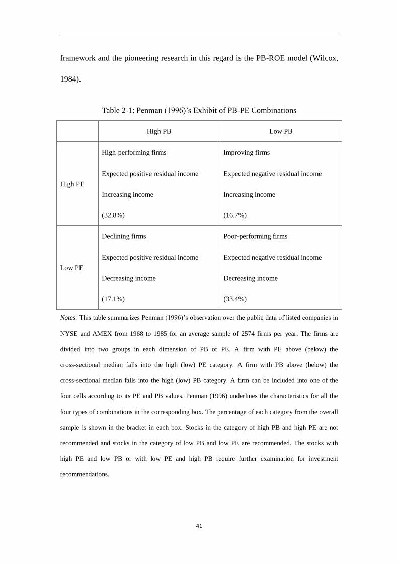
41
framework and the pioneering research in this regard is the PB-ROE model (Wilcox,
1984).
Table 2-1: Penman (1996)’s Exhibit of PB-PE Combinations
High PB Low PB
High PE
High-performing firms
Expected positive residual income
Increasing income
(32.8%)
Improving firms
Expected negative residual income
Increasing income
(16.7%)
Low PE
Declining firms
Expected positive residual income
Decreasing income
(17.1%)
Poor-performing firms
Expected negative residual income
Decreasing income
(33.4%)
Notes: This table summarizes Penman (1996)’s observation over the public data of listed companies in
NYSE and AMEX from 1968 to 1985 for an average sample of 2574 firms per year. The firms are
divided into two groups in each dimension of PB or PE. A firm with PE above (below) the
cross-sectional median falls into the high (low) PE category. A firm with PB above (below) the
cross-sectional median falls into the high (low) PB category. A firm can be included into one of the
four cells according to its PE and PB values. Penman (1996) underlines the characteristics for all the
four types of combinations in the corresponding box. The percentage of each category from the overall
sample is shown in the bracket in each box. Stocks in the category of high PB and high PE are not
recommended and stocks in the category of low PB and low PE are recommended. The stocks with
high PE and low PB or with low PE and high PB require further examination for investment
recommendations.

42
2.2.4 PB-ROE Model
Wilcox (1984)’s PB-ROE model considers PB and ROE in one framework. PB and
ROE can be regarded as the extension of the PE and PB conflict, considering that
ROE=E/B=PB/PE. The dilemma of PE and PB can be restated as that of PB and ROE:
low PB and high ROE is favorable but the fact is that high PB is always associated
with high ROE and low PB is always associated with low ROE. This indicates that
high PB is caused by the expectation that the firm can achieve an abnormally high
ROE. PB and ROE are positively related and such a relation can be theoretically
derived as follows:
The model begins with the identity:
( / )P B P B (2-12)
Take difference on both sides of (2-12)
[ ( / )] ( / ) ( / )P B P B B P B B P B (2-13)
Divide by P on both sides of (2-13)
/ / ( / ) / ( / )P P B B P B P B (2-14)
Define capital return as the sum of price appreciation and dividend payout as:
P D D Pr
P P P
(2-15)
Applying the differential identity:
( / )
/B
D P Br g
P P B
(2-16)
where /Bg B B is the growth rate of book value of equity.
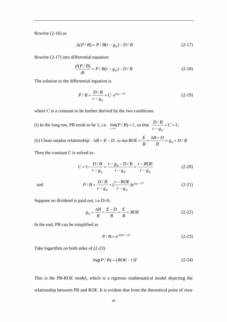
43
Rewrite (2-16) as
( / ) / ( ) /BP B P B r g D B (2-17)
Rewrite (2-17) into differential equation:
( / )/ ( ) /B
d P BP B r g D B
dt (2-18)
The solution to the differential equation is
( )// Bg r T
B
D BP B C e
r g
(2-19)
where C is a constant to be further derived by the two conditions:
(i) In the long run, PB tends to be 1, i.e. ( / ) 1tlim P B
, so that /
1B
D BC
r g
;
(ii) Clean surplus relationship: B E D , so that /B
E B DROE g D B
B B
Then the constant C is solved as:
//1 B
B B B
r g D BD B r ROEC
r g r g r g
(2-20)
and ( )// ( ) Bg r T
B B
D B r ROEP B e
r g r g
(2-21)
Suppose no dividend is paid out, i.e.D=0,
B
B E D Eg ROE
B B B
(2-22)
In the end, PB can be simplified as
( )/ ROE r TP B e (2-23)
Take logarithm on both sides of (2-23)
log( / ) ( )P B ROE r T (2-24)
This is the PB-ROE model, which is a rigorous mathematical model depicting the
relationship between PB and ROE. It is evident that from the theoretical point of view

44
that PB and ROE are positively related. This relationship can also be empirically
determined by the regression model:
log P / B rT T ROE (2-25)
The linear relationship between log (P/B) and ROE can be illustrated in a scatter plot
in a two dimensional framework with log (P/B) on the vertical axis and ROE on the
horizontal axis. Using cross-sectional data, every stock is matched with a pair of ROE
and log (P/B) and the best fit line is the relationship between the two factors. The best
fit line can be viewed as a benchmark for stock valuation. Stocks falling above the
line have high PB but low ROE and thus are overvalued. Stocks falling below the line
have low PB but high ROE and thus are undervalued. The tradeoff rate between log
(P/B) and ROE is the slope T, which is only simply defined investment horizon by
Wilcox. Wilcox does not define the concept of T and this is the research gap that this
paper aims to fill.
The idea of combining PB and ROE is borrowed by Clubb and Naffi (2007), who
actually uses book to market value and future ROE expectations. Their research
shows strong evidence that a simple linear model combining the book-to-market ratio
with expectations of future book-to-market and ROE explains a significant portion of
the cross-sectional variation in future stock returns.
Other models including Estep’s (1985) T-Model and Leibowitz’s (1999) P/E-Orbit
model are developed from Wilcox PB-ROE model, using similar logic. The PB-ROE

45
model differs from both in that its structure more readily invites empirical estimation
of its parameters.
2.3 Premium Payback Period Model
Since the value of a stock is determined jointly by book value of equity (past and
present) and the stock’s earning ability (future), it is useful to determine the
relationship between PB and ROE. Wilcox has provided one version but the slope T in
the equation (2-24) is not well justified. In this part, the core model for this research
Premium Payback Period model is discussed.
2.3.1 Introduction to PPP Model
Stock market price is always higher than the book value per share, so investors always
pay a premium for the opportunity to gain capital return. Buying stocks is like waiting
in a queue, you have to consider: (i) How long is the queue (how much premium to
pay, PB), and (ii) How fast is the queue moving (how profitable is the firm, ROE). As
shown in PB-ROE model, PB and ROE has a positive relation, meaning that the
higher P over B, the bigger ROE is required to recover the premium.
A discreet investor cares how fast his overpaid premium for the stock is compensated
by the capital return, thus is the concept of Premium Payback Period
It is a common phenomenon that stock is sold at premium, i.e. the stock price is
higher than its net book value per share. The investor buys the stock at price which is

46
higher than the book value of equity (P > B). It should be a stupid investment if P is
consistently larger than B. However, the fact is that the asset is earning profit every
year. Assume that no dividend is paid out so that all earning is retained to add to the
book value of equity. Consequently, B is growing bigger. Since the market has the
expectation that the asset is creating value during the period, the market endows the
stock price with a premium over its book value. The premium is reduced with more
profit added to the book value. The investor’s major concern is the final stage when B
levels with P and his investment is paid back. This is called premium payback period
in the stock market. PPP is a good measure to decide how much premium is
reasonable and it should be dependent on ROE.
The existence of premium in the fictitious economy coincides with the proposition
raised in residual income model. Residual income model reveals that the intrinsic
value of a stock equals to the book value of equity and the net present value of
expected residual income. It is also equivalent to Miles’ opinion that the market value
of the company composes of the asset and growth opportunity. When an investor
makes the investment decision of whether to buy the stock, the most crucial factor he
has to consider is whether the premium is acceptable, which is further determined by
the absolute value of the premium and the growth speed of the company’s book value
of equity. The increase in the company’s book value of equity stems from its profit
which is not distributed to shareholders but reinvested in the company. The growth
speed of the increase can be measured by ROE. The safety of a stock investment is
negatively related to premium and positively related to ROE. ROE is a figure which

47
can be derived from the financial report, so that the accounting information is
important in stock investment decision.
In the stock market, the investor buys the fictitious asset at premium over its book
value, in other words, the cost for new shareholders is higher than old shareholders.
What does concern the investor is how soon the premium can be earned back. This is
what called premium payback period is.
2.3.2 Model Construction
Premium payback period can be easily calculated by market data and accounting data.
The key assumptions of PPP model is summarized as below.
Assumption 1: the stock market is inefficient.
Market inefficiency refers to the fact that the prices of stocks do not fully reflect all
the information. Efficient market hypothesis rules out the possibility of an investment
strategy which can generate excess return. Only in the condition of inefficient market,
can an investor have the chance to beat the market with specific investment methods.
In addition, efficient market is valid only under very rigorous conditions, one of
which is investor’s rationality.
Assumption 2: the investors are irrational.
Irrational investors refer to those who make their investment decisions not based on
the fundamentals of the economy and the company, but on the search for the

48
unreleased information. Irrationally investors are easily influenced by the crowd of
investors and cannot invest by their own judgment. Some investors are irrational
because of their lack of education and experience. Other investors choose to be
irrational, because the market provide profit margin for irrational investors and the
traditional financial theories fail in Chinese stock market as discussed in Question 3.
Assumption 3: the ROE of the listed companies are stable.
A stable ROE is crucial for the PPP model which uses current ROE to forecast future
ROE. It is not realistic to assume that future ROEs are equal to current ROE. But it
can be found that companies with high ROE will continue to have high ROE in the
future.
It should rigorously be noted that the ROE is the future earning ability and is not
observable. What is observable is past ROE and current ROE. It is necessary to
empirically investigate the relationship between current ROE and future ROEs. In this
PPP formula, it is assumed that ROE is stable and predictable. A series of studies have
concluded that current ROE is a good predictor for future ROEs. Chung and Jeong
(2000) investigate HK listed stocks and rank all the companies ROE in the bench year
and observe the median ROE in the following five years. They find: first high ROE
will be followed by high ROE and low ROE will be followed by low ROE; secondly
the sectional difference between high and low ROE is getting smaller (mean
reverting). These two findings confirm that ROE is stable and predictable, which is
consistent with the discoveries using US data (Beaver, 1970; Freeman, et al, 1982;

49
Penman, 1993).
I adopted Chung and Kim (2000)’s methodology to test the relationship between
current ROE and future ROE using data from China’s stock market. I investigated the
ROEs of the Shanghai Shenzhen Composite 300 component stocks from 2005 to 2015.
Not all 300 stocks have been staying in the composite from 2005 to 2015 and some
stocks have experienced restructuring. Therefore, the 300 stocks are shortlisted into
180 qualified samples. I choose the year 2005 as a base year and rank all the stocks in
term of their ROE. The 180 stocks are equally divided into 5 classes, where the first
(fifth) class of stocks has the lowest (highest) ROE. The median ROE of each class of
stocks are to be studied for every 2 following years, i.e. 2006-2007, 2008-2009,
2010-2011, 2012-2013, and 2014-2015. It is concluded from Table 2-2 that stocks
with higher (lower) ROE tend to have higher (lower) ROE consistently in the future.
This finding is consistent with the findings in other markets.
Table 2-2: Median ROE for Sample Stocks from 2005-2015
ROE Class 2005 2006-07 2008-09 2010-11 2012-13 2014-15
1 -6.44% 4.36% 5.34% 11.44% 9.31% 6.99%
2 4.34% 6.04% 7.74% 12.41% 8.49% 9.42%
3 8.54% 10.30% 11.37% 13.61% 11.54% 9.23%
4 14.02% 13.78% 12.54% 14.56% 11.62% 13.35%
5 19.44% 21.12% 12.62% 17.48% 13.72% 13.70%
Notes: Table 2-2 shows the evolution of median ROE for sample stocks from 2005 to 2015. The
first class which has the lowest ROE in the base year 2005, also tends to have the lowest median
ROE in the following years. The fifth class which has the highest ROE in the base year 2005 also

50
tends to have the highest median ROE in the following years.
Assumption 4: investors have limited investment opportunities
Limited opportunity for investment ensures that an investor has the only choices over
either the stock or the real asset of the company. This assumption implies that the cost
of capital, or required rate of return, or opportunity cost is equal to zero. Therefore my
PPP model does not have to take into consideration the discount factor.
2.3.2.1 Single Interest Model
Suppose that interest is not compounded, and the premium payback period for a single
stock equals to the paid premium divided by annual earnings per share. The result is
obviously the number of years needed to recover purchase premium.
Price Book Value per SharePPP
Earnings per Share
(2-26)
Note that PE=Price/Earnings per share and ROE=E/B, PPP can be expressed in
simple indicators as:
1PPP PE
ROE (2-27)
The formulation is based on the fact that the price of a stock is higher than its book
value, and the difference between market price and book value is denoted as the
premium (equivalent to the stock price minus book value per share) in this study. The
reason why the investor can accept the premium is that the stock can generate cash

51
flow in terms of earning. The major concern for investment is how long it takes the
earning to compensate the premium. This is how the idea of premium payback period
comes into being.
It is obvious that premium payback period is positively related to the absolute
premium and negatively related to the earning ability. The investor has to make a
tradeoff between premium and earning ability in making investment decisions and the
equilibrium constructs the margin of safety. In the case of the same earning per share,
a higher premium reflects bigger bubble and less desirable investment. In the case of
equal premium, a smaller EPS will result in a longer premium payback period.
2.3.2.2 Compounded Interest Form
Suppose that the earning in each period is reinvested in the company and no dividend
is paid out, thus the compounded interest form of PPP model. Still, the essential
equation is the book value of equity grows up to the purchase price so that the
investment is paid back.
(1 )NP B ROE (2-28)
where P is the stock rice,
B is the book value of equity,
ROE is the return on equity,
N is premium payback period (PPP).
Reshape (2-28) in order to solve N:
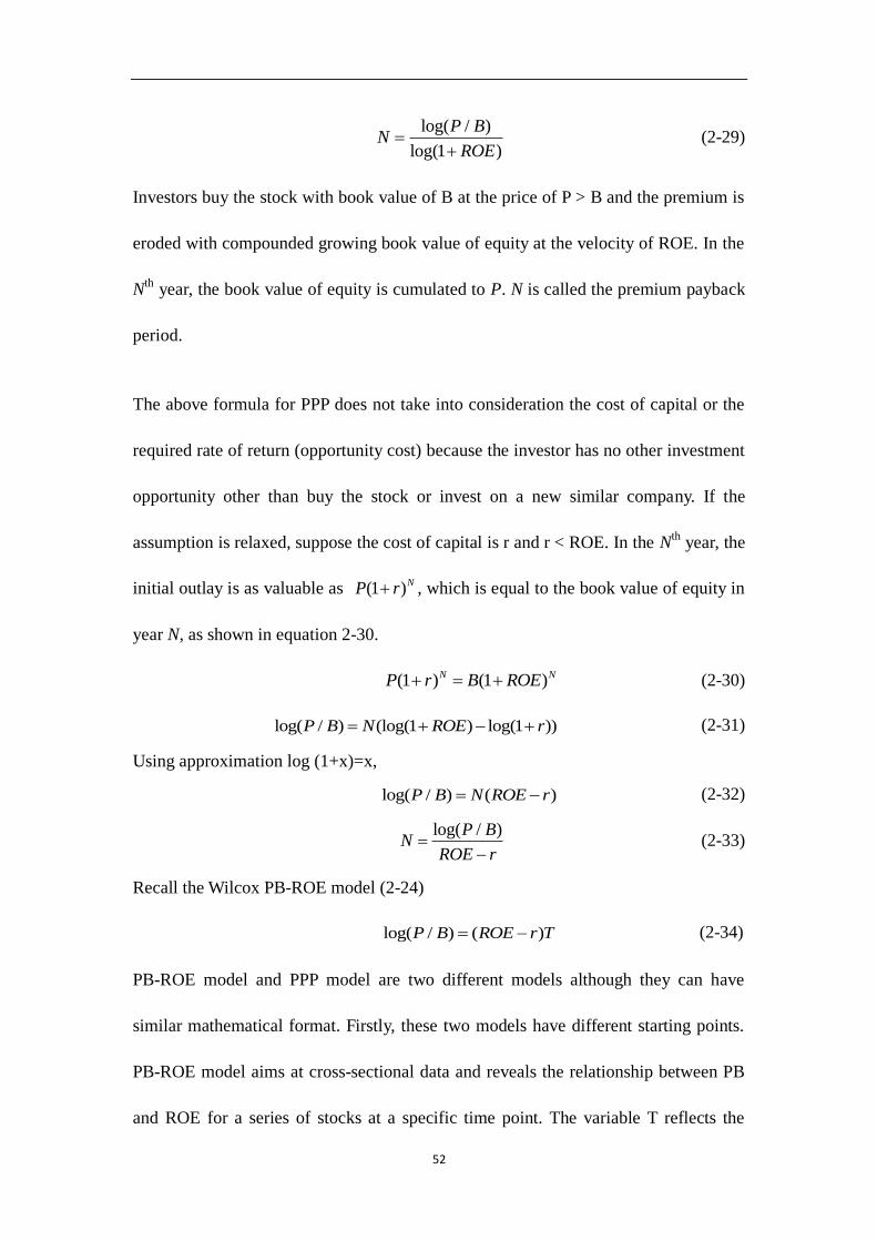
52
log( / )
log(1 )
P BN
ROE
(2-29)
Investors buy the stock with book value of B at the price of P > B and the premium is
eroded with compounded growing book value of equity at the velocity of ROE. In the
Nth
year, the book value of equity is cumulated to P. N is called the premium payback
period.
The above formula for PPP does not take into consideration the cost of capital or the
required rate of return (opportunity cost) because the investor has no other investment
opportunity other than buy the stock or invest on a new similar company. If the
assumption is relaxed, suppose the cost of capital is r and r < ROE. In the Nth
year, the
initial outlay is as valuable as (1 )NP r , which is equal to the book value of equity in
year N, as shown in equation 2-30.
(1 ) (1 )N NP r B ROE (2-30)
log( / ) (log(1 ) log(1 ))P B N ROE r (2-31)
Using approximation log (1+x)=x,
log( / ) ( )P B N ROE r (2-32)
log( / )P BN
ROE r
(2-33)
Recall the Wilcox PB-ROE model (2-24)
log( / ) ( )P B ROE r T (2-34)
PB-ROE model and PPP model are two different models although they can have
similar mathematical format. Firstly, these two models have different starting points.
PB-ROE model aims at cross-sectional data and reveals the relationship between PB
and ROE for a series of stocks at a specific time point. The variable T reflects the

53
relationship. PPP aims at an individual stock and is applied to see whether a stock is
undervalued or overvalued. Secondly, the two models are achieved from different
perspective. PB-ROE model is derived from rigorous mathematical modeling whereas
PPP model is derived from financial instinct. The two differences lead to PPP model’s
superiority to PB-ROE model in the following aspects.
Firstly, the T variable in PB-ROE model is obtained from regression, which is a
statistical concept but the PPP variable is computed for each individual stock, which
is an economic concept. Secondly, in PB-ROE model, the T variable is fixed and each
stock is plotted above or below the line to determine whether it is overvalued or
undervalued. PPP varies for different stocks and its value is signal of overvaluation or
undervaluation. Therefore PPP is a simpler method. Thirdly, PPP model serves as an
important supplement to PB-ROE model in that Wilcox discusses little about the
meaning of slope T and PPP model imposes a very concrete economic meaning for
this variable, and builds a bridge between real and fictitious economies.
In the remaining part of this thesis, I adopt the simplified version of PPP model,
where I assume the cost of capital r is equal to zero for the reason that there is very
limited opportunity for investment that an investor has the only choices over either the
stock or the real asset of the company. Even in the case of the opportunity for
investment in risk free asset, I assume that the return of risk free asset (Rf) is so small
compared with ROE that it can be neglected. Therefore, the discount factor is not
considered.

54
PPP follows the logic of Tobin’s Q in bridging the real and fictitious economies. The P
value is defined as the ratio of PPP in fictitious economy over in real economy as
follows:
PPP in Fictitious Economy
PPPP in Real Economy
(2-35)
When P<1, it means the investment in fictitious economy is more favorable than real
economy and capital will rush into the stock market so that the undervalued stock
price will rise. Contrary, when P>1, investment in real economy is more attractive so
that capital will flow out of stock market. The PPP in fictitious economy is calculated
by my model and the PPP in the real economy is obtained from market observation.
For the latter, the opportunity cost is also neglected, so there is no need to count for
the opportunity cost of the former. The formula applied to compute PPP in this thesis
is equation (2-29).
2.3.3 PPP in Real Economy and Selection of the Critical Value
Like the function of Tobin’s Q in bridging real economy and fictitious economy, the
PPP model can also make the bridge and the comparison between PPP and the critical
value determines the direction of cash flow. Earning is equivalent in every invested
vehicle, and the investor only cares the size of input and output and the speed to
realize the profit.
When the PPP in the fictitious economy is longer than that in the real economy, it is

55
safer to invest in real economy; when the PPP in the fictitious economy is shorter than
that in the real economy, capital investment will flow back to the stock market. PPP in
the fictitious market can be calculated with the formula described previously. PPP in
the real economy can only be observed from the market data available.
Market data shows that a stock’s market price (P) is larger than its book value (B) of
equity. The essence of PPP is the process of B overtaking P. Suppose an investor is
faced with two choices, investing in fictitious economy or real economy. Let’s
examine these two scenarios respectively to see how PPP works.
Suppose the investor enters the fictitious economy and invests P in the stock whose
book value is only B. However, considering the company is earning profit and the
retained earnings is added to the book value of the equity. The accumulation of
earnings increases B to P so that the investment is paid back. PPP for investment in
fictitious economy is time needed to reclaim to nominal loss in a passive way.
Suppose the investor enters the real economy and he establishes a new company at the
cost B. Such an asset is valued at P in the stock market. It seems that the entrepreneur
can sell the company and obtain the quick and easy money (P-B). However, it is not
that soon because it takes time for the company to be recognized by the market before
it completes initial public offering (IPO). Once its value is observed by the market, it
is listed in the stock market. The initial investment of B realizes its potential
worthiness of P. This is also the process of B growing into P. PPP in real economy is
different from that in the fictitious market in that the investor pays active effort to in

56
the management of the company, and the payback period is the time to realize the
potential profit.
PPP in fictitious economy and real economy is comparable. The result of comparison
leads to the decision of investment strategy. PPP in the stock market can be calculated
by the formula 2-29. On the other side, PPP in the real economy can be summarized
from fact observation. PPP in the real economy can be viewed as the timed needed for
a company from establishment to being listed in stock market. I denote it as T.
I use the data from Second-board Market or Growth Enterprise Market (GEM) to
calculate the threshold for PPP mainly because GEM can more accurately simulate
the time required for a company to list in the capital market. China’s GEM was
officially launched in 2009. It was developed for companies which were not entirely
suitable for the main board market. Stocks traded in GEM have the codes starting
with 300. The total market value of GEM reached 55916RMB by the end of 2015.
Compared with main board market, GEM has more relaxed requirements for IPO,
such as establishment date, capital size or long term financial performance. Thus the
threshold for GEM is much lower than the main board market. Normally speaking, it
is easier and takes less time for a company to be listed in GEM than in main board.
Main board market has too many restrictions and the information from it may be
distorted and misleading. So the data gathered from GEM is closer to the reality and
better reflects the PPP value in real economy. This is why GEM stocks are used to
compute the threshold of PPP in real economy.

57
My observation of the data for Growth Enterprise Market starts from 30 October 2009,
when the first stock (code: 300001) in GEM was listed. The GEM data shows the time
span of a company from establishment to IPO. Different companies spend different
numbers of years to achieve the goal. When I first adopted this method, I considered
the top 5% shortest (around 5 years) as a buy threshold, so a stock with a PPP shorter
than 5 years can beat 95% of the companies in real economy in terms of premium
payback period. I considered the median PPP (around 9.5 years) as a sell threshold, so
a tock with a PPP of 9.5 years is beaten by half of the companies in real economy.
This is how the rule of thumb 5 years and 9.5 years came to being. However, when
data continues to accumulate, the threshold does not change much. For the sample
from 2009 to 2015, 5 years ranks top 6% and 9.5 years rank top 44%. Therefore I
stick to the rules of 5 and 9.5 years.
I select 5 years as an entry PPP threshold (buy signal) and 9.5 years as an exit PPP
threshold (sell signal). For the stocks with a PPP < 5 years, they require less time to
get back premium paid than most of firms and it is safe to invest in these stocks. For
the stocks with a PPP > 9.5 years, they require more time to get back premium paid
than nearly half of firms and it achieves average margin of safety.
A large sample of recent data can also justify the critical value established. I collected
the T values for all the companies listed in China’s stock market including Shanghai
Security Exchange and Shenzhen Security Exchange from December 2010 to
February 2016. The number of observations is 781 for the selected period. The max

58
and min Ts for the sample are 35.57 and 0.88, and the median and mean Ts are 11.39
and 11.8 years respectively. 7.17% of the observations have a T shorter than 5 years
and 65% of the observations have a PPP longer than 9.5 years. Therefore, investment
in stocks with PPP < 5 can have a better return than 93% firms in the real economy
and have a satisfactory margin of safety. Stocks with PPP > 9.5 may perform more
poorly than 35% firms in the real economy.
It should be reiterated that the selection of PPP critical values is not an absolute
criterion. It is advised to invest in stocks with low PPP but no one can say how low
PPP is low enough just as in the case of low PE and low PB. The difference between
PPP and relative ratios is that PPP can find its counterpart in the real economy and the
critical value can be reflected in the observations in the real economy. In different
market conditions, the observations in the real economy may be different, for instance
IPO approval process may take longer. In addition, if the PPP criterion is set to be too
strict, it may rule out some potentially good investment targets, because the safest
way to protect investment is to invest in nothing. Therefore the selection of PPP
critical value is the balance between safety and opportunity. The observation in real
economy offers insight for a relative accurate selection of PPP critical value. The buy
signal of PPP < 5 and sell signal of PPP > 9.5 have been used in my own investment
for many years and examined by my investment experience
2.3.4 Comparison of PPP and Tobin’s Q
Different from traditional financial valuation models, the Tobin’s Q theory provides a

59
macroeconomic perspective on the stock valuation. The Q ratio was first proposed by
Tobin (1969) to analyze the relationship between stock price and investment
expenditure. Tobin’s Q stresses replacement cost rather than book value. Replacement
value refers to the amount that a company would have to pay to replace an asset at the
present time, according to its current worth. Replacement cost can be regarded as the
present value of past cost. Tobin’s Q is the ratio of a company’s market value to its
replacement cost. This is a ratio between two valuations. The nominator is how much
the company is worth in the stock and bond market (fictitious economy). The
denominator is how much the company cost if it is rebuilt with current economic
resources (real economy).
Total Market Value of FirmQ Ratio
Total Asset Value of Firm (2-36)
If Q > 1, it is cheaper to build the company than to buy the share of an existing
company, therefore the capital is invested in real economy.
If Q < 1, it is cheaper to directly buy the stock in financial market to have the control
of a company, therefore cash flows into fictitious economy.
Tobin’s Q is a perfect theory, but of little avail to real practice. In theory, Q should
move around 1 but observation from the financial market evidently shows that Q is
fluctuating around some value high above 1. One explanation of why Tobin’s Q is
consistently above 1 is that the denominator is underestimated because
entrepreneurship cannot be fairly valued as an economic resource. Tobin’s Q is the
60
static description of the relationship between financial capital and industrial capital,
neglecting the earning ability. Therefore it is necessary to introduce a earning
dynamics into Tobin’s Q theory so that the theory is still workable when Q is
consistently above 1.
PPP and Tobin’s Q are comparable in that both theories can bridge between real and
fictitious economies and serve as good guidance for investment practice. PPP follows
the residual income model and stresses the value creation in the company business,
while Tobin’s Q only focuses the static replacement cost of the asset. PPP’s value
creation perspective is more realistic and true to fact, so it is more useful for
investment practice.
The critical value is different for the two variables. The critical value for Tobin’s Q is
1, and the comparison between Q and 1 decides the investment decision. The critical
value for PPP is dependent on markets. The payback period may be country-specific.
Comparing PPP and the critical value can also guide the cash flow. PPP is a better tool
for practice.
2.4 Practice of PPP Model and a Pilot Empirical Study
2.4.1 Data Collection
The data used in this research to calculate PPP in fictitious economy is retrieved from
the resource terminal of Shanghai Jushengyuan Data Service Co. The data includes all
the listed companies traded in Shanghai Stock Exchange and Shenzhen Stock

61
Exchange. Daily data is collected ranging from 1 Jan 1991 to 14 Oct 2011. The
Shanghai Stock Exchange and Shenzhen Stock Exchange were established in 1990
and 1991 respectively. Considering data availability, my sample is from 1 July 1992
to 14 Oct 2011. The data types include annual financial report and daily stock price
and earning information.
The date used to calculate PPP in real economy (critical value) is retrieved from the
Growth Enterprise Market in Shenzhen Stock Exchange. The prospectuses of all the
listed companies in this market are reviewed.
According to the theoretical explanations in previous sections, I calculate the PPP for
both fictitious economy and real economy respectively as follows.
2.4.2 PPP Model in Fictitious Economy
PPP can be used to judge whether or not an individual stock is safe as well as the
overall stock market is safe. In this part, I define that the investment in stock market
to hold all the listed companies. The weight of each stock in my portfolio equals to its
weight in the stock market.
Define and compute:
Q: weighted average of PB ratio of the market in one trading day (market Tobin’s Q)
Q=Total Market Value / Total Book Value (2-37)
ROE: weighted average of return on equity in one trading day
ROE=Total annualized income / Total Book Value (2-38)

62
PE: weighted average of PE ratio in one trading day
PE=Total market price / Total annualized income (2-39)
PPP: premium payback period for the overall market
PPP=log(PB )/ log(1+ROE) (2-40)
For non-annual figures, the following methods are applied to yield annualized figures:
(i) For first quarter income data, the annualized data=income*4;
(ii) For second quarter income data, the annualized data=income*2
(iii) For third quarter income data, the annualized data=income*4/3
2.4.2.1 Tobin’s Q in China’s Stock Market
Figure 2-1 is drawn about the Tobin’s Q ratio for the overall market. Evidently,
Tobin’s Q fluctuates widely around 3.5 during the period. One thing worth
mentioning is that Tobin’s Q has never dropped below 1 for the entire period. As
discussed previously, Tobin’s Q can to certain extent provide value judgment for the
investment. The defect is that it does not consider the earning ability of the company.

63
0
1
2
3
4
5
6
7
8
19921210
19930615
19931210
19940616
19941220
19950628
19951226
19960709
19970108
19970724
19980209
19980806
19990204
19990820
20000310
20000912
20010330
20011009
20020423
20021101
20030520
20031124
20040610
20041215
20050705
20060106
20060720
20070125
20070807
20080219
20080821
20090305
20090904
20100318
20100921
20110408
20111014
Q Q_AVER Q_MEDIAN
Figure 2-1: Tobin’s Q in China’s Stock Market
Notes: This figure shows the Tobin’s Q for China’s stock market from 1992 to 2011. The
horizontal axis is time period from 10 December 1992 to 14 October 2011; the vertical axis is the
value for Tobin’s Q; the black curve is the time series plot of Tobin’s Q and the red and blue lines
are respective the average and the median of Tobin’s Q over the entire period. Tobin’s Q fluctuates
widely around 3.5 during the period. One thing worth mentioning is that Tobin’s Q has never
dropped below 1 for the entire period.
2.4.2.2 Premium Payback Period in China’s Stock Market
I construct my ideas of PPP into software called Investment Strategy System Based on
PPP, which is formulated by me to guide my investment. The output of my analysis is
shown in the Figure 2-2.
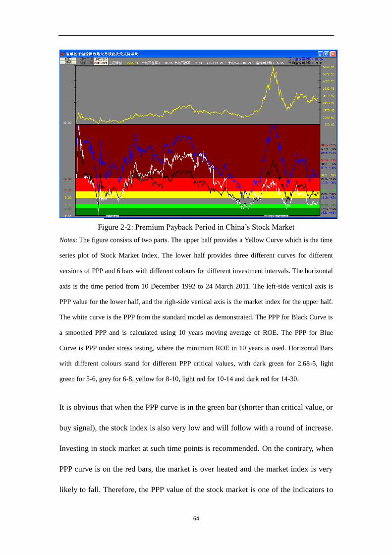
64
Figure 2-2: Premium Payback Period in China’s Stock Market
Notes: The figure consists of two parts. The upper half provides a Yellow Curve which is the time
series plot of Stock Market Index. The lower half provides three different curves for different
versions of PPP and 6 bars with different colours for different investment intervals. The horizontal
axis is the time period from 10 December 1992 to 24 March 2011. The left-side vertical axis is
PPP value for the lower half, and the righ-side vertical axis is the market index for the upper half.
The white curve is the PPP from the standard model as demonstrated. The PPP for Black Curve is
a smoothed PPP and is calculated using 10 years moving average of ROE. The PPP for Blue
Curve is PPP under stress testing, where the minimum ROE in 10 years is used. Horizontal Bars
with different colours stand for different PPP critical values, with dark green for 2.68-5, light
green for 5-6, grey for 6-8, yellow for 8-10, light red for 10-14 and dark red for 14-30.
It is obvious that when the PPP curve is in the green bar (shorter than critical value, or
buy signal), the stock index is also very low and will follow with a round of increase.
Investing in stock market at such time points is recommended. On the contrary, when
PPP curve is on the red bars, the market is over heated and the market index is very
likely to fall. Therefore, the PPP value of the stock market is one of the indicators to

65
predict future movement of the market index.
2.4.3 Determination of PPP Critical Value
We know that the guidance of Tobin’s Q theory is to compare q and 1. For PPP model,
the critical value is more complex. As discussed previously, the critical value for PPP
in stock market can be mapped in the real economy. The benchmark for PPP is how
long the investment in a new company (B) can be recognized by the financial market
as P. This is defined as PPP in real economy and can be measured by the period from
a company’s establishment to going public.
In the fictitious economy, stock investment seems to be a bad decision to buy a stock
valued at P but is only worth B in accounting aspects. However, the purchased asset
can generate net income in the future and the gap between P and B is shrinking.
Suppose no dividend and B will eventually catch up with P at the time point defined
as premium payback period. This is the process of recovering the nominal loss of P-B.
Similarly such a process is also available in real economy and that is why market
observation can correctly show the critical values for PPP model. Suppose an investor
invests in real economy and establishes a company at the cost of B (price in real
economy). A comparable company is valued at P in stock market (price in fictitious
economy). Considering that P is always higher than B, the investor seems to have
potential capital gain by selling the firm in the stock market. In practice, it is not so
easy for a new firm to go public. The investor makes effort to establish fame of the

66
company and receives market recognition, resulting in the IPO of the company. This
is the process of B catching up with P, a process of entrepreneurs’ active practice. The
duration from company’s establishment to IPO can be viewed as the PPP in real
economy, and which is observable from public data in real economy.
The derivation of critical values has been discussed in Section 2.3.3 in detail. It is
easy to compare the PPP in stock market with the benchmark. In my own practice, the
rule of thumb is that PPP < 5 is a good investment opportunity when the stock market
is undervalued, while PPP > 9.5 is a dangerous signal that there is bubble in the stock
market.
2.4.4 Practice of PPP Model for Investment Timing
The Figure 2-2 itself is the best evidence of the effectiveness of PPP investment
strategy. Low PPP (in the green interval) sends an entry signal, when stock index is
also at bottom. However, the effectiveness of PPP model is in question for high PPP.
High PPP means long period to recover the premium and indicates low investment
value so the decision is to exit from market. But Figure 2-2 shows that the index
continues to rise before dropping as the model suggests.
PPP model can capture the overall trend of the market but fail to precisely determine
market peak. This is not the fault of the model, but that of irrational investors. The
model indicates the sell timing, but irrational investors continue to buy in a crazy
manner, thus postponing the falling of the market. Other macro factors such as

67
inflation, interest rate also count.
2.4.5 A Pilot Empirical Study of PPP
In Section 2.4.2, the application of premium payback period model for the whole
stock market in deciding investment timing is demonstrated. In this part, PPP model is
used for selecting individual stocks to compose an investment portfolio. A pilot
empirical test is performed to test the existence of excess returns.
2.4.5.1 Sample Selection for Pilot Study
As a pilot study, this section selects a typical sample according to previous
discussions. I choose the date of 14 May 2004 as the start for my sample observation,
and the 13 May 2005 as the end of the observation.
The purpose of the pilot study in Chapter is only to demonstrate how PPP can be used
as a guide for stock selection. The result of how PPP portfolio performs is not the
primary concern for this part.
The selection of sample period is a bit arbitrage in this case. The above period
coincides with a bear market condition when Shanghai Security Composite Index
dropped sharply from 1595 to 1108 points. I would like to reiterate that the sample is
used to show how PPP is applied, not how well PPP model performs.
The duration of the sample is set to be one year can also be fully discussed. For value
investment, one year seems to be a little short. It takes much time for the market to

68
discover the undervalued stocks.
The total sample under investigation is Shanghai Shenzhen Composite Index 300
(SSCI300) stocks. It is interesting to examine the relationship between PB and ROE
for these 300 stocks at the start point for stock selection.
Figure 2-3: PB-ROE of Shanghai-Shenzhen Composite 300 stocks
Note: This figure presents the PB and ROE for the 300 stocks of Shanghai Shenzhen Composite
Index. The horizontal axis is the ROE value for the stocks. The vertical axis is the PB value for the
stocks. On the whole, stocks with higher ROE tend to have higher PB and most of the
observations fall into the first quadrant. Liner regression test shows that PB is positively related to
ROE. Using the Spearman rank order test for covariance test, PB and ROE are significantly and
positively related and the correlation coefficient is 0.188712 with t value of 2.669635 (at 1%
significance level).
69
2.4.5.2 Stock selection
For value investors, there are many established methods to select stocks. In this pilot
study, I only demonstrate two methods for stock selection. One is the traditional DDM
and the other is my PPP method.
(1) Three Stage DDM Model
This section first applies the three stage DDM model. According to the historical
dividend data and future growth expectations, the intrinsic values of the stocks are
computed to compare with their market prices. Unfortunately, only 4 of the 300 stocks
are available for the rigorous criteria: Price < Intrinsic Value. The four stocks are
BGGF(600019), YTWH(600309), GDNR(600406) and XSPC(600415).
The limited number of investment targets selected by DDM is caused by the special
dividend payout policy in China. China’s stock market is still in the preliminary stage.
The listed companies have not formulated a stable dividend payout policy and even if
they have the dividends are only paid in a small amount. On the other hand investors
are more concerned about the capital gains from change in price than dividend. More
precisely, China’s stock market has three features in terms of dividend policy.
Firstly, Dividend Payout Ratio in China’s stock market is very low. Dividend payout
ratio is the percentage of earnings paid to shareholders in dividends. The dividend
payout ratio is highly related to the company's level of maturity. A new,
growth-oriented company that aims to expand would be expected to reinvest most or

70
all of its earnings and could be forgiven for having a low payout ratio. I have
reviewed the dividend payout history of SSCI300 composite stocks since their IPO.
Only 56 stocks (18.73%) claim to have an average dividend payout ratio above 50%.
70% of the stocks have an average dividend payout ratio below 40%.
Secondly, Dividend Yield Ratio in China’s stock market is very low. Dividend yield
ratio is a financial ratio that measures the amount of cash dividends distributed to
common shareholders relative to the market value per share. I also studied the
dividend yield ratio of the SSCI300 composite stocks and I used the lowest price in
the year to calculate the dividend yield ratio. Even though this treatment may
overestimate the dividend yield ratio, the overall performance is still very low. Only
30 stocks (10%) claim to have an average dividend yield ratio over 3.5%. 60% of
stocks have an average dividend yield ratio below 2%. A low ratio may indicate that
the stocks are overvalued.
Thirdly, dividend policy for China’s listed companies is not stable. I refer to stable
dividend policy as a company pays out dividend at least in 9 years (including 9 years)
out of the past 10 years. I refer to unstable dividend policy as a company pays out
dividend at most in 7 years (including 7 years) out of the past 10 years. The
percentage of stable and unstable dividend policies in China is plotted in Figure 2-4.

71
Figure 2- 4 Percentage of stable and unstable dividend policies in China
Notes: Figure 2-4 shows the percentage of listed companies which have stable (blue) and unstable
(red) dividend policies. It is obvious that on the whole trend, the proportion of companies with
stable dividend policy is increasing. Despite the improvement in the dividend policy, stable
dividend policy only accounted for 47.83% in 2015, still at a very low level.
The above three features result in undervaluation of stocks by dividend. Therefore
very few stocks can be selected by DDM.
Even though these 4 stocks can be confirmed as undervalued stocks, the insufficient
numbers of stocks can be an obstacle for huge investment. Big trading volumes will
easily influence the market price of the stocks. Therefore DDM model is not useful in
practice.
(2) PPP method
Similarly, PB, ROE are first calculated to yield the final PPP indicators for each
individual stock using the formula (2-41):
PPP = log (P/B) / log (1+ROE) (2-41)

72
Table 2-3: Summary Statistics for PPP of 300 stocks
Mean 9.67
Standard Deviation 12.62
Median 7.03
Min -43.87
Max 73.33
Notes: This table reports the summary statistics for PPP of the sample stocks of SSCI300.
Statistics show that PPP values of the sample stocks have a wide range and the mean and median
are 9.67 and 7.03 respectively. The wide range of PPP makes this indicator efficient to sort the
sample stocks.
According to section 2.3.3, the observations in the real economy indicate that majority
of companies have a PPP longer than 5 years. Therefore, the stocks with PPP shorter
than 5 years are selected. The critical value of 5 years is very high standard, but still
60 stocks out of 300 are available for this criterion, providing many investment
opportunities with limited market influence.
2.4.5.3 Jensen’s α Test for Excess returns
Jensen's α, which was first used as a measure in the evaluation of mutual fund
managers in Jensen (1968), is commonly used to determine the excess return of a an
asset over the theoretical expected return. The asset could be a stock or a portfolio of
stocks. The theoretical return, which is risk adjusted, is predicted by a market model
and the most commonly adopted model is the capital asset pricing model (CAPM).
According to an equilibrium perspective, a riskier asset should have a higher expected
return than a less risky asset. When an asset’s return is higher than the risk adjusted

73
return, then the asset is believed to have excess return or positive α.
The Jensen alpha test is the regression model:
, , , , ,( )i t f t i i M t f t i tR R R R (2-42)
where,i tR is the daily return for stock i at time t. i can also be a portfolio.
,M tR is the daily return of market portfolio at time t.
,f tR is the return of risk free asset, represented by current deposit rate.
i is the intercept to be estimated and is expected to be 0 if no excess return
occurs.
i is the slope to be estimated and is regarded as an indicator for relative
systematic risk.
,i t is the error term of unsystematic risk with the expected mean of zero.
According to CAPM,
, , , ,( )i t f t i M t f tR R R R (2-43)
The intercept α in the regression model should be 0. If α > 0 and is significant, excess
return occurs, or stock i provides a return over risk-adjusted return. If α < 0, negative
excess return occurs. The pilot study focuses on the alpha value of the stocks selected
by PPP model.
2.4.5.4 Empirical Results of Jensen’ s α Test
(1) Excess return test for individual stocks
The market index (Shanghai Shenzhen Composite 300) fell from 1239 to 887 points

74
by 28.41% in the year from 14 May 2004 to 13 May 2005. In such a bear market
condition, most of the 60 selected stocks also witnessed negative return. However,
only 12 stocks were beaten by the market, and the other 48 stocks boasted of their
returns higher than -28.41%.
To test the significance of the excess return, the Jensen’s α test regression model is
run for all the 60 selected stocks individually to test the sign and significance of the
intercept α. I employ the econometric package of Eviews 7.0 to obtain the regression
results shown in Table 2-3. Most “α”s are positive, (49/60); only 11 “α”s are negative.
Some “α”s are significantly positive at 5% level (11/60).
Table 2-4: Summary of regression for portfolio composites
No. Stock Code Stock Name IPO Date PPP 1y return α
1 000039.SZ ZJJT 1994-4-8 2.57 0.9015 0.004217**
2 000059.SZ TLHG 1997-1-30 3.48 -0.0319 0.001411
3 000063.SZ ZXTX 1997-11-18 3.14 0.2137 0.001979
4 000527.SZ MDDQ 1993-11-12 3.02 0.1496 0.001679
5 000623.SZ JLAD 1996-10-28 1.08 0.0904 0.001882
6 000629.SZ PGFT 1996-11-15 1.51 -0.2628 -8.17E-05
7 000630.SZ TLYS 1996-11-20 4.19 -0.3035 0.000206
8 000651.SZ GLDQ 1996-11-18 4.79 0.0138 0.001253
9 000709.SZ HBGT 1997-4-16 1.42 -0.0823 0.000685
10 000729.SZ YJPJ 1997-7-16 3.30 -0.1052 0.000278
11 000768.SZ XFGJ 1997-6-26 1.24 -0.1958 0.000271
12 000778.SZ XXZG 1997-6-6 2.82 -0.2160 0.000131
13 000807.SZ YLGF 1998-4-8 3.64 -0.4381 -0.000929
14 000825.SZ TGBX 1998-10-21 1.67 -0.1269 0.000713
15 000858.SZ WLY 1998-4-27 1.21 0.0596 0.001319
16 000876.SZ XXW 1998-3-11 2.11 -0.1754 0.000854
17 000898.SZ AGGF 1997-12-25 1.99 -0.0340 0.001315
18 000933.SZ SHGF 1999-8-31 4.60 -0.0340 0.00109
19 000937.SZ JZNY 1999-9-9 3.75 0.2901 0.002163*
20 000960.SZ XYGF 2000-2-21 4.49 0.1525 0.002631*
21 000961.SZ ZNJS 2000-3-1 3.40 -0.4580 -0.000947

75
No. Stock Code Stock Name IPO Date PPP 1y return α
22 000983.SZ XSMD 2000-7-26 4.15 0.3312 0.002573*
23 600005.SH WGGF 1999-8-3 3.34 0.1197 0.002111
24 600009.SH SHJC 1998-2-18 4.25 0.3350 0.001907*
25 600010.SH BGGF 2001-3-9 2.34 -0.1579 0.000524
26 600019.SH BGGF 2000-12-12 3.03 -0.1851 0.000173
27 600026.SH ZHFZ 2002-5-23 4.46 0.1359 0.001821
28 600058.SH WGFZ 1997-5-28 4.15 -0.1103 0.001241
29 600066.SH YTKC 1997-5-8 1.27 0.0204 0.001096
30 600068.SH GZB 1997-5-26 1.13 -0.4517 -0.001081
31 600096.SH YTH 1997-7-9 3.12 0.1363 0.001703
32 600098.SH GZGG 1997-7-18 4.21 -0.2444 0.000271
33 600108.SH YSJT 1997-8-18 1.48 -0.4133 -0.000418
34 600111.SH BGXT 1997-9-24 4.54 -0.4085 -0.000179
35 600125.SH TLWL 1998-5-11 4.36 0.5015 0.002932*
36 600151.SH HTJD 1998-6-5 4.61 -0.4708 -0.000741
37 600153.SH JFGF 1998-6-16 3.24 -0.2588 0.000215
38 600170.SH SHJG 1998-6-23 3.30 -0.3364 -0.000455
39 600177.SH YGE 1998-11-19 1.00 -0.0118 0.001214
40 600188.SH YZMY 1998-7-1 4.59 -0.1294 0.000591
41 600219.SH NALY 1999-12-23 3.58 -0.3458 -0.000298
42 600307.SH JGHX 2000-12-20 2.09 -0.2258 0.000324
43 600320.SH ZHZG 2000-12-21 3.56 0.2880 0.0028688*
44 600331.SH HDGF 2001-12-20 0.80 0.5890 0.003585*
45 600352.SH ZJLS 2003-8-1 4.39 0.0068 0.001357
46 600362.SH JXTY 2002-1-11 4.60 -0.2628 0.000415
47 600380.SH JKY 2001-6-8 4.17 -0.1880 0.000207
48 600418.SH JHQC 2001-8-24 4.16 -0.2800 0.000302
49 600428.SH ZYHY 2002-4-18 3.95 0.3758 0.00308*
50 600500.SH ZHGJ 2000-3-1 3.58 -0.0014 0.001599
51 600508.SH SHNY 2001-8-29 4.60 -0.0242 0.001375
52 600519.SH GZMT 2001-8-27 3.81 0.7063 0.002901**
53 600690.SH QDHE 1993-11-19 2.52 -0.2530 7.33E-05
54 600694.SH DSGF 1993-11-22 4.84 0.3114 0.002323*
55 600795.SH GDDL 1997-3-18 3.24 -0.2388 0.000169
56 600808.SH MGGF 1994-1-6 2.85 -0.3225 -0.000148
57 600811.SH DFJT 1994-1-6 4.93 -0.3097 0.000348
58 600839.SH SCCH 1994-3-11 1.28 -0.3752 -0.000384
59 600859.SH WFJ 1994-5-6 4.62 -0.0773 0.000899
60 600881.SH YTJT 1995-11-15 1.97 -0.2611 0.000225
Notes: This table shows the regression results for the 60 stocks selected by PPP model. The stock
name and code selected are displayed in Columns 2 and 3. Column 4 shows the IPO dates of the

76
60 stocks. Column 5 shows the calculated values of PPP for the stocks and it is evident that all the
selected stocks have PPP values shorter than 5 years. Column 6 is the one year buy-and-hold
return from 14 May 2004 to 13 May 2005, and only 21 stocks have positive return over the period
of bear market environment. The last column shows the Jensen α for each regression using the
software Eviews 7. The α value is the indication for excess returns. Most “α”s are positive, (49/60);
only 11 “α”s are negative. Some “α”s are significantly positive at 5% level (11/60).
* indicates significant at 5% level;
** indicates significant at 1% level.
(2) Excess return test for PPP portfolio
The PPP portfolio is an average weighted portfolio of all the 60 stock selected by PPP
criterion. The statistical summary of the daily return for both market index and PPP
portfolio are shown in the Table 2-4 and most statistics are very similar except the
mean return.
Table 2-5: Comparison of Market Index and PPP Portfolio Returns
Summary Statistics Market Index PPP Portfolio
Mean -0.001195 -0.000211
Median -0.001933 -0.001300
Maximum 0.053290 0.052300
Minimum -0.039915 -0.046600
Std. Dev. 0.013492 0.013618
Skewness 0.866386 0.688350
Kurtosis 4.454646 4.391414
Notes: This table compares market index return with PPP portfolio return for the one year holding
period from 14 May 2004 to 13 May 2005. The market index refers to SSCI300. The PPP
Portfolio refers to the portfolio of 60 stocks which have a PPP <5. The PPP portfolio has a higher
mean return and median return than the market index.
Considering that 49 PPP stocks beat the market for the selected investment period,

77
there is every reason to believe that the overall performance of the portfolio excelled
the market performance. The one year return for the portfolio from 14 May 2004 to 13
May 2005 is -6.19%, much higher than market return of -28.41%.
Figure 2-5: Cumulative returns for market index and PPP portfolio
Notes: This figure plots the one year cumulative returns for market index (SSCI300) and PPP
portfolio starting from 14 May 2004. The horizontal axis is the time line and the vertical axis is
the cumulative return. Obviously, the portfolio performance was consistently better than the
market.
For a rigorous statistical test, the α test regression is also performed with the
regression results of the portfolio return shown as follows:
, , , ,0.000965 0.984086( )p t f t M t f tR R R R (2-44)
(4.9415) (68.11128)
where Rp,t is the daily return of the PPP Portfolio at date t.
The R square is 0.9506 with F-statistic at 4639. It is evident that PPP model can help
identify a portfolio that can produce a daily excess return of 0.0965%. The advantage

78
of PPP over DDM in stock selection is that PPP can provide more investment
opportunities and more stocks are recommended. This is very crucial for huge volume
trading.
2.4.5.5 Other empirical studies remaining
The pilot study for empirical research is a useful attempt. Many other tests can be
attempted. First, this pilot study chooses a period of bear market, so that future
empirical test can choose market data at both market highs and market lows, so that
the validity of PPP model can be verified in various market conditions. Second, this
pilot study examines the excess return in one year scope, so future studies can expand
the investment horizon to 3 years or even 5 years to evaluate the long-term
performance of PPP model. Thirdly, if long term investment is investigated, the
composition of PPP portfolio should be dynamically changeable so that new qualified
stocks are bought and disqualified stocks are eliminated from the portfolio. Fourthly,
include other statistical tests to show whether PPP models can create excess returns.
Fifthly, consider external factors which may affect the robustness of PPP and give a
solid theoretical explanation why PPP can create excess return.
2.5 Conclusions
Value investing is a relatively long-term investment, searching for undervalued
high-growth securities in the market. Many valuation models have been developed to
determine the intrinsic value of the stock so that it is easy to tell whether it is

79
over-valued or under-valued. The purpose of this study is to provide a new method for
the same motivation.
The Premium Payback Period model inherits the advantages of the existent models.
PPP takes into consideration the book value of the stock and it also looks ahead to
account for the company’s value creation in terms of ROE. More importantly it is
very easy for application.
Like Tobin’s Q theory, PPP can also serve as a bridge between fictitious economy and
real economy. Investors can decide where to invest their money and their object is to
minimize payback period for safety purposes. A rational investor can judge between
the PPPs in these two economies and finally decide his investment. The PPP for the
fictitious economy can be easily computed by two important ratios PB and ROE
which are readily available in the market. On the other hand, PPP for real economy
requires experiment. Fortunately, the opening of Growth Enterprise Market provides
adequate observation samples to measure the PPP in the real economy as duration
from the establishment and IPO of the company. Observations in real economy and
my investment experience tell that a stock with PPP < 5 years is a good opportunity
for investment.
PPP model is useful in many areas. Firstly, PPP can be applied to the whole market to
examine whether the overall market is bull or bear. The PPP of the whole stock
market can be a signal of timing for market entry or exit. PPP model is also powerful
for investors in selecting stocks for their portfolio. According to the pilot study, PPP

80
model picks 60 stocks out of 300 stocks and empirical test shows that 12 of the stocks
can produce excess return and the averaged-weighted portfolio can also generate
excess return.

81
Chapter 3 Practice of PPP in Stock Investment: A Perspective in Stock Selection
3.1 Introduction
Previously in Chapter 2, a new method, PPP model for valuing individual stocks was
introduced to determine whether a stock is overvalued or undervalued. PPP model
inherits the advantages of the existent models by taking into consideration the book
value of the stock and the company’s earning ability measured in terms of ROE. The
concept of premium payback period is proposed to measure how soon the premium
paid in purchasing stocks is compensated by company earnings. Stocks with low PPP
are safer and more profitable investment target than those with high PPP. My
investment experience shows that normally stocks with PPP shorter than 5 years can
be viewed as value stocks and can generate excess return. This is a very useful rule of
thumb to select stocks and more importantly this criterion leaves abundant stocks for
investment, unlike DDM which is so strict that rules out majority of stocks. PPP
model is also powerful for investors in selecting stocks for their portfolio. According
to the pilot study, PPP model picks 60 stocks out of 300 stocks and the empirical test
shows that 12 of the stocks can produce excess return and the average-weighted
portfolio can also generate excess return. In a nutshell, PPP model assists in selecting
undervalued stocks and allocates investment capital in these stocks for excess return.
The pilot study in Chapter 2 shows a great potential of applying PPP model to stock
investment, but it is to some extent too simplified. The practice of PPP in stock

82
investment can be investigated from two aspects. First of all, how PPP model
performs in different market conditions? Pilot study in Chapter 2 analyzed how PPP
performed in the period from 14 May 2004 to 13 May 2005 and the result was
satisfying. In this chapter, the different market conditions are to be investigated both
the bull and bear markets. Secondly, how can PPP stock selection method collaborate
with other methods to yield better returns? It is common sense that one foot alone
cannot walk far and it is always beneficial to have two or more tools to tackle with the
irrational stock market in China. The exclusive use of PPP may cause some trouble. In
this chapter, the selection in terms of market capitalization is also taken into
consideration. These two new progresses improve the pilot study in Chapter 2 and
demonstrate the power of PPP model in stock selection.
In order to evaluate PPP under different market conditions, two periods are selected.
One period is from 5 Nov 2008 to 3 Nov 2009, which is a period of bull market
condition. The other period is from 5 Dec 2011 to 3 Dec 2012, which is a period of
bear market. On the other development, the selection of stocks takes into account both
its market capitalization and premium payback period. Past experience and theoretical
studies show that stocks with smaller market capitalization tend to yield better returns
than those with larger market capitalization, which is defined as size effect. According
to Chapter 2, stocks with lower PPP tend outperform those with high PPPs, which can
also be defined as PPP effect in this study. In this chapter, the interaction of size effect
and PPP effect is studied under different market conditions.

83
The rest of the chapter is arranged as follows. In section 3.2, I provide a literature
review on size effect and PB effect in stock returns. In section 3.3, I demonstrate the
methodology for this empirical investigation. In section 3.4, I focus on the bear
market condition and present how size effect and PPP effect perform in bear market.
In section 3.5, I concentrate on the bull market and illustrate how size effect and PPP
effect perform in bull market. Section 3.6 is the conclusion for this chapter.
3.2 Literature Review
The focus of this chapter is to identify stocks which are more likely to have better
returns. There have already been several indicators for stock selection. Two of the
most widely recognized indicators are the capitalization and book to market equity.
Their potential to achieve excess return is called size effect and value effect
respectively.
3.2.1 Size Effect
The size effect in finance literature refers to the fact that firms with smaller size have
higher return than those with larger size on average over long horizons. It also
describes the contribution that company size has in explaining stock returns. The size
effect is first proposed by Banz (1981) in testing the Capital Asset Pricing Model. His
research examines the relationship between the total market value of a company’s
stock and its return, using sample stocks in New York Stock Exchange from 1926 to
1975. Using regression, he observes that that stock returns are explained by its size in
addition to market risk adjusted return explained by CAPM model. In one word,

84
market capitalization is a significant factor in explaining stock returns and there is an
inverse relationship between size and returns. The plausible explanation of size effect
is that smaller firms tend to be riskier than larger firms and this additional risk must
be rewarded in term of stock returns. Although Reinganum (1983) and Fama and
French (1992) also proved the existence of size effect, some other scholars are
skeptical to size effect. Schwert (2002) pointed out that size effect is on the trend of
shrinking. Dimon and Marsh (1999) also believes that size effect is fading away and
in some cases reversed, i.e. larger firms have better returns. Goyal and Welch (2003)
denies the so called size effect and advocates that it is the result of sample selection
bias.
The empirical studies on China’s stock market however present similar conclusions
that size effect exists in Chinese stock markets (Wang and Zhou, 2002; Xie and Luo,
2005; Hilliard and Zhang, 2015).
3.2.2 Value Effect
The value effect in finance literature refers to the fact that firms with higher value
have higher return than those with lower value on average over long horizons, where
value is defined the ratio of the company’s book value to price of the stock, or the
inverse of PB ratio. The book to market ratio was first made popular by Ben Graham.
However, it lost popularity when Efficient Market Hypothesis was developed. It
gained back its position especially when Stattman (1980) and Rosenberg, Reid and
Lanstein (1985) unveiled the positive relationship between stock return and book to

85
market ratio. Fama and French (1992) also discovered their significantly positive
relation in US stock market.
The empirical studies on China’s stock market however lead to different conclusions
using different methods and samples. Some researchers do not find evident support
for value effect (Gu and Ding, 2003), Hilliard and Zhang, 2015) while others confirm
significant evidence of value effect (Chen, Zhang and Chen, 2001)
3.2.3 PPP Effect
PPP effect is a concept proposed by me. It has similar definition as size effect in that
stocks with lower PPP tend to perform better than those with higher PPP. The logic is
simple and has been thoroughly discussed in Chapter 2. PPP refers to the time needed
for an investor to recover the overpaid price of the stock’s book value of net asset. A
stock with low PPP is a safe investment because the time to earn back the premium is
short and such a stock is usually undervalued. Investing in stocks with low PPP can
generate considerable return, which may not be explained by CAPM model. The
additional return is supposed to be caused by PPP effect.
Considering that the computation of PPP involves the factor of PB, it is well
considered that PB effect is included in PPP effect. Therefore the framework of size
and PPP effects are sufficient.

86
3.3 Methodology of Empirical Study
The empirical study of PPP effect in acquiring excess return can be segmented into
the following six steps, which will be discussed respectively in this chapter.
Step 1: Determining a sample pool for investigation.
Step 2: Calculating PPP of the sample on a specific bench date.
Step 3: Classification of sample stocks in terms of market capitalization and PPP.
Step 4: Computing daily returns for the categorized portfolios for a specific period.
Step 5: Obtaining Jensen alpha for the portfolios.
Step 6: Evaluating the best performing portfolio and investment recommendation.
3.3.1 Determining a sample pool for investigation.
Since the establishment of Shanghai Securities Exchange and Shenzhen Securities
Exchange in early 1990s, China’s stock market has undergone a remarkable
development in the past two decades. Thousands of stocks have been listed in the two
stock exchanges in Shanghai and Shenzhen. It is unrealistic to evaluate all the stocks
listed. The scope of interest in this chapter is focused on the 300 composite stocks for
Shanghai Shenzhen Composite Index 300 (hereafter referred to as “SSCI300”).
SSCI300 index was first published on 8 April 2005 jointly by the two stock exchanges
to reflect the overall market situation in the China’s A share stock market. The

87
objective to propose such an index is to show price movement and performance of the
entire Chinese stock market, so that it is often used as evaluation bench market for
fund performance. The composite stocks in the SSCI300 index are selected from
different industries and their market capitalization account over 60% of the overall
stock market. Therefore, the index can to some extent represent the overall stock
market. Using the index composites as research sample is feasible and well-grounded.
However, not all 300 stocks in the index can serve as qualified sample. Two additional
conditions are set to screen the stocks. One condition is positive net asset, otherwise
PPP is not applicable. The other condition is that the company is listed for more than
five years, so that the operations and financial ratios are subject to less volatility. The
final sample is thus reduced to short list of around 200 stocks. More specifically, the
sample is shortlisted to 212 stocks for the bear market condition and to 188 stocks for
the bull market condition.
3.3.2 Calculating PPP on a specific date
Since PPP can be used to observe whether a stock is overpriced or underpriced, it is
an important and effective criterion for stock selection. The calculation of PPP is
crucial and the fundamental for further analysis. PPP, by its name, means the period
required for an investment in stock i to achieve additional return so that the price paid
over its book value is earned back.
In the compounded interest form of PPP model, it is supposed that all the earning for a
stock in each period is reinvested in the company and no dividend is paid out. Still,

88
the essential equation is the book value of equity grows up to the purchase price so
that the investment is paid back.
In practice, stocks with PB < 1 are always preferable because an investor pays less
price than the accounting value of the stock. However such ideal stocks are rare in the
stock market. More commonly, investors buy the stock with book value of B at the
price of P > B with the expectation that the premium is shortened with compounded
growing book value of equity at the speed of ROE. In the Nth
year, the book value of
equity is increased to P, where the time this process takes is called the premium
payback period.
Theoretically, PPP can be calculated at any time for a stock, if we know its price,
book value and the ROE. Price of a stock is frequently quoted in the stock market and
it is widely available. Book value is an accounting term and can be found in the
financial report of a listed company, no matter in annual report or quarterly reports.
Unlike price and book value, ROE seems to be more challenging and entails more
precise prediction, because in the model, ROE refers to the profitability in the future.
However, statistics have shown that the ROE of a company is relatively stable so that
past ROE can be used for prediction of the future ROE. So once the price, book value
and ROE are determined, the index of PPP is readily available.
The index of PPP fluctuates with stock price every day. The dynamics of PPP contains
the information of valuation of a stock. A stock’s PPP can compare with an absolute
value for a certain period. For instance, in a relatively long period, PPP lower than

89
five years can be observed as a good opportunity and triggers investment in the stock.
A stock’s PPP can also compare with other stocks on a specific date. For example, on
one particular date, stocks with relatively lower PPPs may have better investment
values. In the pilot study in Chapter 2, the former comparison is applied and the
investment in a series of stocks with PPP lower than 5 years is proved with excess
return. In this chapter, however, the latter comparison is used. The comparison date
can either be random or deliberately chosen.
In this study, a specific date as a bench date to calculate PPP index will be selected for
starting date for different market conditions.
3.3.3 Classification of sample stocks in terms of size and PPP
The shortlisted sample of SSCI300 composite stocks is further divided into particular
portfolios in terms of size and PPP. Market capitalization is used to measure size of a
stock.
According to market capitalization, all stocks are equally divided into three categories.
The stocks with market capitalizations ranking for the largest trisection are labeled as
large size. The stocks with market capitalizations ranking for the smallest trisection
are labeled as small size. The stocks with market capitalizations ranking for the mid
trisection are labeled as mid size.
On the other dimension, all the stocks are also ranked in terms of PPP. All the stocks
can be divided into 2 or 3 categories according to PPP. For the 2 categories, all stocks

90
are divided into two equal categories of high PPP and low PPP. The stocks with PPP
ranking for the higher half are labeled as high PPP. The stocks with market
capitalizations ranking for the lower half are labeled as low PPP. For the 3 categories,
all stocks are not equally divided. Stocks with PPP < 5 are labeled as low PPP; stocks
with PPP > 9.5 are labeled as high PPP; stocks with PPP between 5 and 10 are labeled
as mid PPP.
Therefore all the stocks are labeled in terms of two dimensions. Stocks which fall into
the same category constitute an investment portfolio. Two scenarios may occur for
different classification on PPP. A 3x2 scenario refers to 3 size ranks and 2 PPP ranks
and 6 portfolios are constructed namely (1) large size and high PPP, (2) large size and
low PPP, (3) mid size and high PPP, (4) mid size and low PPP, (5) small size and high
PPP, (6) small size and low PPP.
Similarly, if the stocks are divided into three categories according to high PPP, mid
PPP and low PPP, different stocks which are labeled in terms of size and PPP can be
classified into 9 portfolios, which is the 3x3 scenario. Both the 3x2 and 3x2 scenarios
will be discussed for the performance of each portfolio in later empirical analysis.
3.3.4 Computing daily returns for the categorized portfolios
For each category based on size and PPP, the daily return for every stock can be
computed by the formula:
Rt = ln (Pt / Pt-1 ) (3-1)

91
where Rt is the return for day t,
Pt- is the close price of the stock on day t,
ln is the natural logarithm with the base of e to capture the compound rate form
of return.
The holding period or the duration of investment is determined to be one year for
several reasons. First of all, ROE as an element in PPP is usually calculated on annual
basis so that PPP tends to be relative stable within one year. For duration over one
year, the PPP criteria may indicate different stocks to be included in an investment
portfolio. On the other hand, shorter duration than one year is unsuitable for value
investors who do not frequently buy and sell stocks. The holding period of one year is
an ideal and eclectic option.
Therefore, the above Rt is calculated for a consecutive year. Suppose each portfolio is
equally weighted so that the return of the portfolio is the arithmetic average of its
components, i.e.
, ,
1
1 n
p t i t
i
R Rn
(3-2)
where R p,t is the daily return for the portfolio p on date t,
Ri,t is the daily return for stock i on date t.
The daily return of the portfolio can be compared with the daily return of the market
Rm, which is defined as the daily return of SSCI300 index. The statistical summary of
the discrepancy (Rp – Rm) will be reported and tested.

92
3.3.5 Obtaining Jensen α for the Portfolios
Even though (Rp – Rm) is tested to be significantly different from zero, it may be
caused by the risk factor. In other words, the reason why Rp is consistently larger than
Rm is because Rp bears more systematic risks. Only when the return is adjusted by the
bearing risks, can the final conclusions of excess return be drawn.
Unlike the event study where a potential structural change takes place before or after
the specific date, the date chosen in this PPP test is arbitrage, having no relationship
with any special event. In other words, no structural change occurs for the selected
stocks and there is no concrete argument that the return before and after the date
should be significantly different. One can choose t, t-1 or t+1 freely. In this regard,
such event study methods are not helpful.
The more suitable analytical framework for this study is the Jensen alpha test based
on CAPM equation. Constitute a regression model as:
, , , , ,( )i t f t i i M t f t i tR R R R (3-3)
,i tR is the daily return for stock i at time t. i can also be a portfolio.
,M tR is the daily return of market index (SSCI300).
,f tR is the daily return of risk free asset, represented by current deposit rate.
i is intercept to be estimated and is expected to be 0 if no excess return occurs.
i is slope to be estimated and is regarded as an indicator for relative systematic risk.
,i t is the error term of unsystematic risk with expected mean of zero.

93
According to standard Asset Capital Pricing Model,
, , , ,( )i t f t i M t f tR R R R (3-4)
The intercept α in the regression model should be 0. If α > 0 and is significant, excess
return occurs, or stock i provides a return over risk-adjusted return. If α < 0, excess
loss occurs. Both the sign and significance of α is examined to determine the direction
and magnitude of excess return.
3.3.6 Evaluating the best performing portfolio and recommendations
In both 3x2 scenario and 3x3 scenario, the performance of each portfolio is to be
assessed in comparison with the market return and with each other. The comparison of
portfolio performance with market performance is feasible with the model of Jensen
alpha to check whether a particular portfolio can achieve excess return or not.
The performance comparison with each other is made by comparing the different
Jensen α across different portfolios. Portfolios with positive and large Jensen α are
more attractive for investors, indicating that investing in such portfolios is quite safe
and profitable. Portfolios with Jensen α also have their value because selling short
such portfolios can also achieve excess return. Another implication of comparing
Jensen α is to investigate the effect of size and PPP on portfolio performance. As rule
of thumb, small size stocks and low PPP size stocks are more preferable, but this
hypothesis should be tested under different market conditions.

94
3.4 Size Effect and PPP Effect in Bear Market Conditions
3.4.1 Data Selection and Description
A bear market is defined as a condition in which securities prices fall and widespread
pessimism causes the stock market's downward spiral to be self-sustaining. Investors
anticipate losses as pessimism and selling increases. Although figures vary, a
downturn of 20% or more from their 52-week high in a stock index is considered an
entry into a bear market.
For the chosen period from 5 Dec 2011 to 3 Dec 2012, the SSCI300 index peaked at
2717.78 points and closed at its bottom of 2018.85 points. The index was fallen by
22.4% from peak to bottom and therefore this period was defined as a bear market.
In China there is no such long period of bearish and a common phenomenon is that
the market is on the trend of falling with little sign of rebound. The period under
investigation is characterized by gloomy global market conditions and domestic tight
monetary policy environment.
Potential stocks are selected from 300 index composites. The two criteria have
already been demonstrated that (1) the stock has been listed for more than five years,
(2) book value of equity is positive, otherwise PPP = log (P/B) / log (1+ROE) is
meaningless. By these two criteria the 300 stocks are reduced to 212 stocks available
for investment. The bench date is 5 Dec 2011 for PPP calculation.

95
The 212 stocks exhibit a wide range of PPP from -24.6 to 151.8 years. The negative
PPPs refer to the stocks with P/B<1, so that log (P/B) is negative. Low PPPs are
favorable and negative PPPs are even more favorable because these stocks are sold at
discount instead of premium. The mean of PPP is 10.39 years and the median of PPP
is 6.34 years. A substantial proportion of the stocks are undervalued using the PPP < 5
criteria.
The size of the 212 stocks also shows a wide range of market capitalization from 7.9
billion RMB to 1494 billion RMB. The mean of size is 45.6 billion RMB and the
median is 20 billion RMB. The standard deviation of size is 125 billion RMB.
It is an interesting idea to examine the relationship between size and PPP.
Theoretically, there is no direct or apparent link between size and PPP. A linear
regression between PPP and log (size) offers a surprising result. The size of a stock is
treated with logarithm to become smoother. Regressing PPP against log (size) shows
to what extent size can affect PPP or how these two factors coincide. The regression
result is shown below:
PPP = 32.89 – 4.08 * log (size) (3-5)
(4.23) (-2.96)
The relationship between PPP and size is negative. The coefficients are significant at
1% level. It is directly interpreted as that the stocks with large size tend to have low
PPP and small sized stocks tend to have high PPP.
The impact of size on PPP can be decomposed into PB and ROE. Large size
96
companies are likely to have low PB compared to small size companies. Firstly the
information of large companies is more transparent, so the large size stocks are more
likely to be rationally priced. Secondly, the prices of large stocks are more difficult to
be manipulated. Large size companies are likely to have high ROE compared to small
size companies. Firstly, large companies have economics of scale. Secondly large
companies are usually SOEs who have special advantage over private companies.
Referring to my sample, the median PB for the large size sample is 2.41, smaller than
its counterpart of small size sample (2.65). The median ROE for the large size sample
is 20.09%, larger than is counterpart of small size sample (12.17%).
It can be viewed from an equilibrium perspective. If stocks with large size have high
PPP, the demand for such stocks are low, so there will be adjustments in the stock
market. Therefore stocks with large size are matched with low PPP. Similarly, if small
sized stocks have low PPP, the demand for such stocks is very strong and triggers the
purchase of such stocks. On the other hand, low PPP stocks are desirable and the
overbuying of such stocks make its size grow big.
3.4.2 Investment Portfolios based on 3x2 scenario of size and PPP
3.4.2.1 Portfolio Constituents
When all the stocks are divided into 3 equal categories by size factor and 2 equal parts
by PPP factor, the stocks can fall into one of the six portfolios. Out of 212 stocks,
large size, mid size and small size stocks account respectively for 70, 71 and 71

97
stocks. More specifically, when the size classification cointegrated with PPP
classification, 6 portfolios are constructed.
Table 3-1: Sample Numbers in 3x2 Scenario in Bear Market
High PPP Low PPP Total
Large size 35 35 70
Mid size 36 35 71
Small size 36 35 71
Total 107 105 212
Notes: This table shows the number of stocks in each portfolio matrix. The total sample includes 212
stocks. The sample size for each portfolio is roughly the same, around 35 stocks in each.
3.4.2.2 Average PPP for each portfolio
In order to have an initial impression of how well each portfolio would perform, the
average PPP is calculated for each portfolio. Portfolios with low PPP average are
more likely to have better performance than those with high PPP average. Illustrated
in Table 3-2, the portfolios of the high PPP show much higher PPP indicators (over 10
years) than their low PPP counterparts (within 5 years). On the whole, the PPP value
for the large size, mid size and small size are 5.74 years, 11.94 years and 13.37 years.
Table 3-2: Average PPP for Each Portfolio in 3x2 Scenario in Bear Market
High PPP Low PPP Overall average
Large size 9.35 2.23 5.74
Mid size 19.32 4.43 11.94
Small size 23.71 2.73 13.37
Overall average 17.46 3.13 10.295
Notes: This table shows the average PPP for each portfolio. High PPP portfolios have a much greater

98
PPP value than low PPP portfolios. On the whole, PPP value is negatively related to capitalization size.
3.4.2.3 Statistics of daily returns of portfolios
In this 3x2 scenario analysis, 6 portfolios are constructed in terms of size and PPP.
The summary statistics for the returns of market index and 6 portfolios are computed
in this section.
Table 3-3: Summary Statistics for Market Return and Portfolio Return in Bear Market
Portfolios Mean Median Maximum Minimum Std. Dev. Skewness Kurtosis
SSCI300 -0.00074 -0.0011 0.0478 -0.0288 0.01229 0.558184 4.216362
LH -0.00175 -0.0027 0.0563 -0.0407 0.014234 0.331771 4.389969
LL -0.00068 -0.0008 0.0433 -0.0282 0.01152 0.648884 4.303316
MH -0.00166 -0.0016 0.0548 -0.0395 0.014787 0.271795 3.852184
ML -0.00105 -0.00165 0.0558 -0.0416 0.014981 0.217651 4.004931
SH -0.00188 -0.00155 0.0608 -0.046 0.016296 0.101034 3.874513
SL -0.00083 -0.00125 0.059 -0.0434 0.015851 0.280822 3.697976
Notes: This table displays the summary statistics for the daily returns of market index (SSCI300) and 6
portfolios. The six portfolios are named by LH for large size and high PPP, LL for large size and low
PPP, MH for mid size and high PPP, ML for mid size and low PPP, SH for small size and high PPP,
SL for small size and low PPP. The daily return for each portfolio is calculated and the average returns
are all negative, because during this period, the overall stock market index also dropped slightly. All
the average daily returns for the six portfolios except LL portfolio are lower than market return.

99
3.4.2.4 Test of Excess Return by Jensen α
For each of the six portfolios, the following regression is performed to test the sign
and significance of the intercept α.
, , , , ,( )p t f t p p M t f t p tR R R R (3-6)
,p tR is the daily return for a portfolio, which can be LH, LL, MH, ML, SH or SL.
,M tR is the daily return of market portfolio (SSCI300).
,f tR is the daily return of risk free asset, represented by current deposit rate.
p is intercept to be estimated and is expected to be 0 if no excess return occurs.
p is slope to be estimated and is regarded as relative systematic risk.
,p t is the error term of unsystematic risk with the expected mean of zero.
Table 3-4: Regression Results of 6 Portfolios in 3x2 Scenario in Bear Market
No. Portfolio α β
1 Large Size and High PPP (LH) -0.000936**
(-2.9609)
1.087550**
(42.2846)
2 Large Size and Low PPP (LL) -0.000018
(-0.0979)
0.905566**
(57.9257)
3 Mid Size and High PPP (MH) -0.000820**
(-2.3809)
0.054452**
(40.0611)
4 Mid Size and Low PPP (ML) -0.000207
(-0.5593)
1.126166**
(37.3945)
5 Small Size and High PPP (SH) -0.000964*
(-2.2994)
1.216107**
(35.6454)
6 Small Size and Low PPP (SL) 0.000102
(0.3323)
1.230787**
(49.4522)
Notes: This table displays the regression results for the 6 portfolios return against market return.
Eviews 7.0 is applied to generate the results. The estimatedαandβare shown in the table and the
corresponding t values are displayed in the bracket.
* indicates significant at 5% level;
** indicates significant at 1% level.

100
The focus of study is Jensen alpha of the regression. Notably, the Jensen alphas for
the high PPP groups regardless of size are all significantly negative; investing in high
PPP portfolios may probably lead to unfavorable results regardless the size of stocks
selected. For the low PPP group, Jensen alphas are all insignificant, and the only the
small sized group show a positive sign. Still, it is worth noting that for either high PPP
or low PPP group, portfolio with small-sized stocks tends to perform better than
portfolio with large-sized stocks. In the bear market, PPP effect seems to be more
eminent than size effect.
Table 3-5: Jensen alpha for Size-PPP portfolios in Bear Market
High PPP Low PPP
Large size -0.000936** -1.88E-05
Mid size -0.000820* -0.000207
Small size -0.000964* 0.000102
Notes: This table reorganizes Table 3-4 into PPP-size matrix. The figures presented in the boxes
are the Jensen α for the six combinations. Portfolios with high PPP all have negative excess return.
* indicates significant at 5% level;
** indicates significant at 1% level.
3.4.2.5 Investment Recommendations
Based on the Jensen alpha test for excess return, there are two investment
recommendations of the bear market period. The first recommendation is to strongly
avoid investing in high PPP stocks. The second recommendation is to invest in the
small capitalization stocks with low PPP.

101
Considering the fact that PPP effect is more influential than size effect in bear market,
a new portfolio can be constructed solely based on PPP criterion regardless of their
size. The new portfolio consists of buying the low PPP portfolios and selling the high
PPP portfolios. The initial investment amount for the new portfolio is zero because the
long and short positions offset each other. The return of the new portfolios, which can
be defined as Low Minus High portfolio (hereafter LMH), can be computed below:
RLMH = RLowPPP - RHighPPP (3-7)
where RLowPPP is the average daily return for all the 105 stocks which are labeled as
low PPP, and RHighPPP is the average daily return for all the 107 stocks which are
labeled as high PPP.
Jensen alpha model can also be applied to test the performance of the LMH portfolio
against market return.
LMH: RLMH – Rf = 0.000765 – 0.054452* (RM – Rf) (3-8)
(2.2603) (-1.9767)
Jensen alpha is significantly positive at 5% level. It is evident that the LMH portfolio
can obtain excess return and is thus an effective investment.
The above LMH portfolio can be further improved by taking into consideration the
size effect. Since the performance of a stock is negatively related to its size, it is
advisable to buy the stocks of small size and low PPP (long SL portfolio) and sell the
stocks of large size and high PPP (short LH portfolio). The SL portfolio and LN

102
portfolio are on the diagonal of Table 3-1, therefore I name this new portfolio
diagonal portfolio, donated as D.
RD = RSL - RLH (3-9)
Jensen alpha model can also be applied to test the performance of the diagonal
portfolio against market return.
D Portfolio: RD – Rf = 0.000938 + 0.143236* (RM – Rf) (3-10)
(2.3007) (4.31967)
Jensen alpha for D portfolio is 0.000938, which significantly positive at 5% level and
it is also larger than the Jensen alpha in LMH portfolio (0.000765). It is evident that
the diagonal portfolio can obtain excess return and also improves LMH portfolio.
3.4.3 Investment Portfolios based on 3x3 scenario of size and PPP
3.4.3.1 Portfolio Constituents
When all the stocks are divided into 3 categories by size factor and 3 categories by
PPP factor, the stocks can fall into one of the nine portfolios. When the size
classification co integrated with PPP classification, 9 portfolios are constructed, and
the number of stocks in each portfolio is shown in the Table 3-6.
Table 3-6: Sample Numbers in 3x3 Scenario in Bear Market
High PPP Mid PPP Low PPP Total
Large size 10 25 35 70
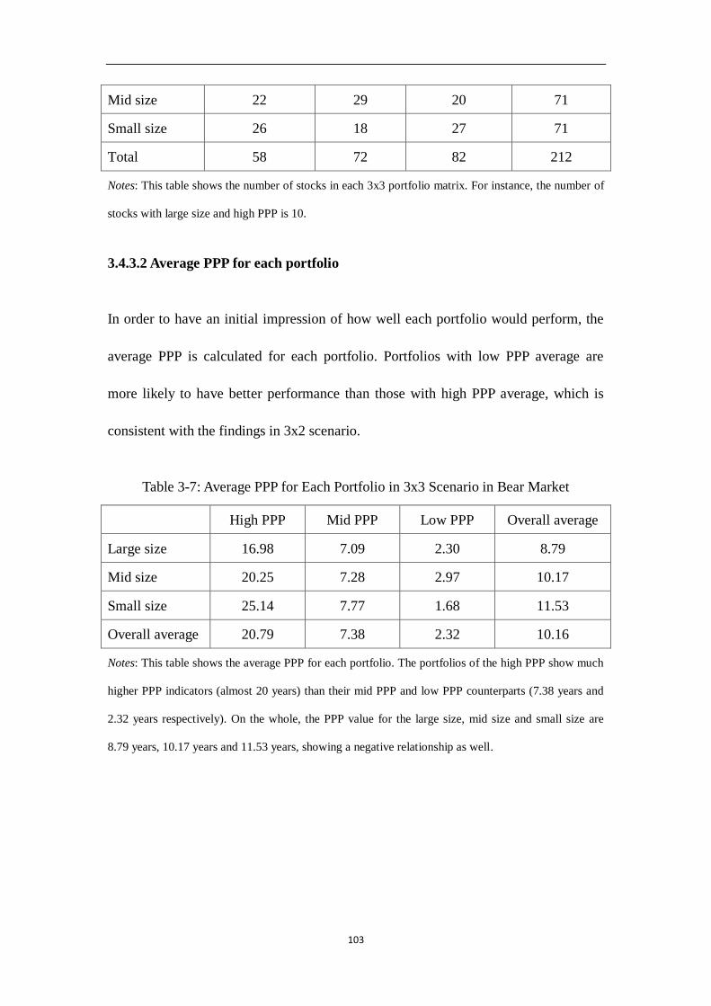
103
Mid size 22 29 20 71
Small size 26 18 27 71
Total 58 72 82 212
Notes: This table shows the number of stocks in each 3x3 portfolio matrix. For instance, the number of
stocks with large size and high PPP is 10.
3.4.3.2 Average PPP for each portfolio
In order to have an initial impression of how well each portfolio would perform, the
average PPP is calculated for each portfolio. Portfolios with low PPP average are
more likely to have better performance than those with high PPP average, which is
consistent with the findings in 3x2 scenario.
Table 3-7: Average PPP for Each Portfolio in 3x3 Scenario in Bear Market
High PPP Mid PPP Low PPP Overall average
Large size 16.98 7.09 2.30 8.79
Mid size 20.25 7.28 2.97 10.17
Small size 25.14 7.77 1.68 11.53
Overall average 20.79 7.38 2.32 10.16
Notes: This table shows the average PPP for each portfolio. The portfolios of the high PPP show much
higher PPP indicators (almost 20 years) than their mid PPP and low PPP counterparts (7.38 years and
2.32 years respectively). On the whole, the PPP value for the large size, mid size and small size are
8.79 years, 10.17 years and 11.53 years, showing a negative relationship as well.

104
3.4.3.3 Statistics of daily returns of portfolios
In this 3x3 scenario analysis, 9 portfolios are constructed in terms of size and PPP.
The summary statistics for the returns of market index and 9 portfolios are computed
in this section.
Table 3-8: Summary Statistics for Market Return and Portfolio Return in Bear Market
Portfolios Mean Median Maximum Minimum Std. Dev. Skewness Kurtosis
SSCI300 -0.00074 -0.0011 0.0478 -0.0288 0.01229 0.558184 4.216362
LH -0.00144 -0.00215 0.0574 -0.0396 0.014072 0.469273 4.527958
LM -0.00144 -0.00215 0.0574 -0.0396 0.014072 0.469273 4.527958
LL -0.00074 -0.0009 0.0448 -0.0285 0.011791 0.666219 4.381685
MH -0.00131 -0.0013 0.0537 -0.0407 0.015054 0.179144 3.662154
MM -0.00137 -0.00145 0.0617 -0.052 0.015845 0.35171 4.379365
ML -0.00104 -0.0017 0.0551 -0.0427 0.014917 0.215319 3.930187
SH -0.00179 -0.00095 0.0608 -0.0519 0.016322 0.080576 3.962602
SM -0.00179 -0.00145 0.0627 -0.0499 0.017438 0.094434 3.591933
SL -0.00067 -0.00135 0.0573 -0.0432 0.015573 0.250414 3.762716
Notes: This table displays the summary statistics for the returns of market index (SSCI300) and 9
portfolios. The nine portfolios are named by LH for large size and high PPP, LM for large size and mid
PPP, LL for large size and low PPP, MH for mid size and high PPP, MM for mid size and mid PPP,
ML for mid size and low PPP, SH for small size and high PPP, SM for small size and mid PPP, SL for
small size and low PPP. The daily return for each portfolio is calculated and the average returns are all
negative, because during this period, the overall stock market index also dropped slightly. Almost the
average daily returns for the nine portfolios are lower than market return.

105
3.4.3.4 Test of Excess Return by Jensen α
For each of the nine portfolios, the following regression is made to test the sign and
significance of the intercept.
, , , , ,( )p t f t p p M t f t p tR R R R (3-11)
,p tR is the daily return of portfolio LH, LM, LL, MH, MM, ML, SH, SM or SL.
,M tR is the daily return of market index SSCI300.
,f tR is the daily return of risk free asset, represented by current deposit rate.
p is the intercept to be estimated and is expected to be 0 if no excess return occurs.
p is slope and is regarded as an indicator for relative systematic risk.
,p t is the error term of unsystematic risk with an expected mean of zero.
Table 3-9: Regression Results of 9 Portfolios in 3x3 Scenario in Bear Market
No. Portfolios α β
1 Large Size and High PPP (LH) -0.000650
(-1.9688)
1.066741
(39.7027)
2 Large Size and Mid PPP (LM) -0.000650
(-1.9688)
0.905566
(39.7027)
3 Large Size and Low PPP (LL) -0.000027
(-0.1418)
0.930640
(60.7356)
4 Mid Size and High PPP (MH) -0.000465
(-1.2599)
1.133264
(37.7665)
5 Mid Size and Mid PPP (MM) -0.000427
(-1.501023)
1.238439
(53.5104)
6 Mid Size and Low PPP (ML) -0.000195
(-0.5399)
1.124732
(38.1885)
7 Small Size and High PPP (SH) -0.000874
(-2.0275)
1.211854
(34.5536)
8 Small Size and Mid PPP (SM) -0.000823
(-1.6625)
1.274499
(31.6543)
9 Small Size and Low PPP (SL) 0.000232
(0.7214)
1.200556
(45.8665)
Notes: This table displays the regression results for the 9 portfolios return against market return.

106
The estimated α and β are shown in the table and the corresponding t values are displayed in the
bracket.
* indicates significant at 5% level;
** indicates significant at 1% level.
Notably, the Jensen alphas for the high PPP groups are significantly negative;
therefore investing in high PPP portfolios is very likely to lead to unfavorable results
regardless the size of stocks selected. For the low PPP group, Jensen alphas are all
insignificant, and the only the small size portfolio show a positive sign. Table 3-10
shows the Jensen alphas for the nine portfolios.
Table 3-10: Jensen alpha for Size-PPP portfolios in Bear Market
High PPP Mid PPP Low PPP
Large size -0.000650* -0.000650* -2.67E-05
Mid size -0.000465 -0.000427 -0.000195
Small size -0.000874* -0.000823 0.000232
Notes: This table reorganizes Table 3-9 into PPP-size matrix. The figures presented in the boxes
are the Jensen alphas for the 9 combinations.
* indicates significant at 5% level;
** indicates significant at 1% level.
3.4.3.5 Investment Recommendations
Based on the Jensen alpha test of excess return, there are two investment
recommendations of the bear market period. The first recommendation is to strongly
avoid investing in high PPP stocks. The second recommendation is to invest in the
small capitalization stocks with low PPP. There is no material difference from the

107
recommendations in 3x2 scenario.
Following the same method in 3.4.2.5, a new portfolio can be constructed from the
available portfolios by buying the low PPP portfolios and selling the high PPP
portfolios. The initial input of the new portfolio is zero because the long and short
positions offset each other. The return of the new portfolios, which can be called low
minus high portfolio (LMH), can be computed below:
RLMH = RLowPPP - RHighPPP (3-12)
where RLowPPP is the average daily return for all the 82 stocks which are labeled as low
PPP, and RHighPPP is the average daily return for all the 58 stocks which are labeled as
high PPP.
Jensen alpha model can also be applied to test the performance of the LMH portfolio
against market return.
LMH: RLMH – Rf = 0.000566 –0.051977* (RM – Rf) (3-13)
(1.6622) (-1.8752)
Jensen’s α is positive but not significantly positive. In this case the LMH portfolio
cannot obtain excess return.
Similarly, the diagonal portfolio can be constructed by buying SL portfolio and selling
LH portfolio.
RD = RSL - RLH (3-14)
Jensen’s α model can also be applied to test the performance of the diagonal portfolio

108
against market return.
D Portfolio: RD – Rf = 0.000782 + 0.122815* (RM – Rf) (3-15)
(1.6365) (3.4407)
Jensen’s α in D portfolio is improved compared with that in LMH portfolio, but it is
only significant at 10% level. It cannot conclude excess return for D portfolio at 5%
significance level. It can be explained that stock selection alone cannot ensure excess
return for bear market condition.
In the empirical investigation of the bear market from 5 Dec 2011 to 3 Dec 2012, 212
sample stocks from Shanghai Shenzhen Composite 300 Index are examined in terms
of size and PPP. An inverse relationship between PPP and log(size) is discovered. The
inverse relationship can be explained from an equilibrium perspective. Large size
stocks tend to have lower PPP and small size stocks tend to have higher PPP. Two
scenarios of size-PPP combinations (i.e. 3x2 and 3x3) are respectively investigated,
and both scenarios conclude similar statistical results. In bear market, PPP effect is
more dominant than size effect in that portfolios with different PPPs show sharp
contrast return result but the returns across different size categories show no
significant difference. Therefore, in bear market, an investor should be more keen to
selecting stocks by means of PPP as a priority criteria. An investor should avoid
stocks with high PPPs and is advised to invest in small firms with low PPP. A good
recommendation of effective investment is LMH portfolio (buying low PPP stocks
and selling high PPP stocks) or D portfolio (buying SL portfolio and selling LH

109
portfolio).
3.5 Size Effect and PPP Effect in Bull Market Conditions
3.5.1 Data Selection and Description
A bull market is defined as a condition in which securities prices rise and widespread
optimism causes the stock market’s upward spiral to be self-sustaining. Investors
anticipate gains as optimism and buying increases. Although figures vary, an upturn of
20% or more from their 52-week low in a stock index is considered an entry into a
bull market.
For the chosen period from 5 Nov 2008 to 3 Nov 2009, the SSCI300 index started at
bottom of 1627.76 points and climbed to the peak of 3787.03 points during the sample
period. The index rose by 32.6% from bottom to peak and therefore this period was
defined as a bull market.
This period is characterized by bullish market conditions in domestic stock market as
well other assets market such as real estate market.
Again, potential stocks are selected from 300 index composites. Because of different
timing, the 300 composites are not completely identical to the index in Section 3.4.
The two criteria have already been demonstrated. The first criterion is that the stock
has been listed for more than five years. The second criterion is that book value of
equity is positive, otherwise PPP = log (P/B) / log (1+ROE) is not computable. By
these two criteria the 300 stocks are shortlisted to 188 stocks available for investment.

110
The bench date is 5 Nov 2008.
The 188 stocks exhibit a wide range of PPP from -152.7 to 160.8 years. The negative
PPPs refer to the stocks with P/B<1, so that log (P/B) is negative. Low PPPs are
favorable and negative PPPs are even more favorable because these stocks are sold at
discount instead of premium. During the selected bullish market period, 29 stocks
exhibit negative PPP, indicating high investment value. The mean of PPP is 6.78 years
and the median of PPP is 4.78 years. A substantial proportion of the stocks are
undervalued using the PPP < 5 criteria. From the first glance of the PPP of the stocks,
this period is very likely to be bull market.
The size of the 188 stocks also show a wide range from 0.3 billion RMB to 587
billion RMB. The mean of size is 18.5 billion RMB and the median is 7.5 billion
RMB. The standard deviation of size is 48.1 billion RMB.
It is an interesting idea to examine the relationship between size and PPP.
Theoretically, there is no direct or apparent link between size and PPP. A linear
regression between PPP and log (size) offers a surprising result again. The size of a
stock is treated with logarithm to become more smooth. Regressing PPP against log
(size) shows to what extent size can affect PPP or how these two factors coincide. The
regression result is shown below:
PPP = 16.7488 – 2.2591 * log (size) (3-16)
(2.7332) (2.6816)
The relationship between PPP and size is negative. The coefficients are significant. It

111
is directed interpreted as that the stocks with large size also tend to have low PPP and
small sized stocks tend to have high PPP in bull market. It can be viewed from an
equilibrium perspective. If large sized stocks have high PPP, the demand for such
stocks are low, so there will be adjustments in the stock market. Therefore large sized
stocks are matched with low PPP. Similarly, if small sized stocks have low PPP, the
demand for such stocks is very strong and triggers the purchase of such stocks. On the
other hand, low PPP stocks are desirable, and the overbuying of stocks with low PPP
pushes up its price and makes its size grow big.
3.5.2 Investment Portfolios based on 3x2 scenario of size and PPP
3.5.2.1 Portfolio Constituents
When all the stocks are divided into 3 equal parts by size factor and 2 equal parts by
PPP factor, the stocks can fall into one of the six portfolios. Table 3-11 shows the
number of stocks in each portfolio matrix.
Table 3-11: Sample Numbers in 3x2 Scenario in Bull Market
High PPP Low PPP Total
Large size 33 31 64
Mid size 30 33 63
Small size 29 32 61
Total 92 96 188
Notes: This table shows the number of stocks in each portfolio matrix. The total sample includes 188
stocks. The sample size for each portfolio is roughly the same.

112
3.5.2.2 Average PPP for Each Portfolio
In order to have an initial impression of how well each portfolio would perform, the
average PPP is calculated for each portfolio. Portfolios with low PPP average are
more likely to have better performance than those with high PPP average. Illustrated
in the Table 3-12, the portfolios of the high PPP show much higher PPP indicators
(over 10 years) than their low PPP counterparts (within 2 years). On the whole, the
PPP value for the large size, mid size and small size are 5.51 years, 6.38 years and
8.12 years, showing a negative relationship between PPP and capitalization.
Table 3-12: Average PPP for Each Portfolio in 3x2 Scenario in Bull Market
High PPP Low PPP Overall average
Large size 10.79 0.22 5.51
Mid size 11.09 1.66 6.38
Small size 15.64 0.60 8.12
Overall average 12.51 0.83 6.67
Notes: This table shows the average PPP for each portfolio. High PPP portfolios have a much greater
PPP value than low PPP portfolios. On the whole, PPP value is negatively related to capitalization size.
3.5.2.3 Statistics of daily returns of portfolios
In this 3x2 scenario analysis, 6 portfolios are constructed in terms of size and PPP.
The summary statistics for the returns of market index and 6 portfolios are computed
in this section.

113
Table 3-13: Summary statistics for market return and portfolio returns in Bull Market
Portfolios Mean Median Maximum Minimum Std. Dev. Skewness Kurtosis
SSCI300 0.003075 0.0044 0.0712 -0.0771 0.022926 -0.490111 4.164834
LH 0.001855 0.0036 0.0579 -0.066 0.019659 -0.549731 4.09533
LL 0.003168 0.0045 0.0773 -0.0852 0.024179 -0.425163 4.157312
MH 0.003109 0.0064 0.0609 -0.076 0.02263 -0.667203 4.25831
ML 0.004103 0.0063 0.0809 -0.0863 0.026695 -0.530965 4.077175
SH 0.004524 0.007 0.0684 -0.0743 0.023974 -0.616198 4.102336
SL 0.004703 0.0074 0.0759 -0.0789 0.026318 -0.602781 4.227612
Notes: This table displays the summary statistics for the returns of market index and 6 portfolios. The
six portfolios are named by LH for large size and high PPP, LL for large size and low PPP, MH for mid
size and high PPP, ML for mid size and low PPP, SH for small size and high PPP, SL for small size
and low PPP. The daily return for each portfolio is calculated and the average returns are all positive,
because during this period, the overall stock market index also surged rapidly. All the average daily
returns for the six portfolios are higher than market return except the LH portfolio.
3.5.2.4 Test of Excess Return by Jensen α
For each of the six portfolios, the following regression is made to test the sign and
significance of the intercept.
, , , , ,( )p t f t p p M t f t p tR R R R (3-17)
,p tR is the daily return for a portfolio, which can be LH, LL, MH, ML, SH or SL.
,M tR is the daily return of market portfolio (SSCI300).
,f tR is the daily return of risk free asset, represented by current deposit rate.
p is the intercept to be estimated and is expected to be 0 if no excess return occurs.

114
p is the slope to be estimated and is regarded as an indicator for relative systematic
risk.
,p t is the error term of unsystematic risk with expected mean of zero.
Table 3-14: Regression Results of 6 Portfolios in 3x2 Scenario in Bull Market
No. Portfolio α β
1 Large Size and High PPP (LH) -0.000645
(-1.49)
0.806629
(43.05)
2 Large Size and Low PPP (LL) -0.000002
(-0.0069)
1.031878
(73.48)
3 Mid Size and High PPP (MH) 0.000277
(0.514)
0.918348
(39.39)
4 Mid Size and Low PPP (ML) 0.000706
(1.329)
1.108106
(48.10)
5 Small Size and High PPP (SH) 0.001445*
(2.2242)
0.945347
(32.83318)
6 Small Size and Low PPP (SL) 0.001611*
(2. 4254)
1.061509
(37.709)
Notes: This table displays the regression results for the 6 portfolios return against market return.
Eviews 7 is applied to generate the results. The estimated α and β are shown in the table and the
corresponding t values are displayed in the bracket.
* indicates significant at 5% level;
** indicates significant at 1% level.
Notably, the Jensen’s α for the large size groups are negative, investing in large size
portfolios may probably lead to unfavorable results regardless their PPP values. For
the mid size group, Jensen’s αs are positive but not significant, because in this bull
market, the market index has already in a quick increase, it is less likely for common
stocks to beat the entire bull market significantly. Still, it is worth noting that for the
small size group, both high PPP and low PPP portfolios perform better than portfolio
with large-sized stocks. Size effect is more dominant than PPP effect. For the small
sized group, portfolio with low PPP seems to slightly out beat high PPP, although both

115
can generate excess return over the entire market. Table 3-15 shows the Jensen alphas
for the six portfolios. Portfolios with small sizes all have positive excess return.
Table 3-15: Jensen alpha for size-PPP portfolios in Bull Market
High PPP Low PPP
Large size -0.000645 -2.25E-06
Mid size 0.000277 0.000706
Small size 0.001445* 0.001611*
Notes: This table reorganizes Table 3-14 into PPP-size matrix. The figures presented in the boxes
are the Jensen alphas for the six combinations. Portfolios with small sizes have positive excess
return.
* indicates significant at 5% level;
** indicates significant at 1% level.
3.5.2.5 Investment Recommendations
Based on the Jensen alpha test of excess return, there are two investment
recommendations of the bull market period. The first recommendation is to strongly
avoid investing in large capitalization stocks. The second recommendation is to invest
in the small capitalization stocks with low PPP.
Considering the fact that size effect is more influential than PPP effect in bull market,
a new portfolio can be constructed solely based on size criterion regardless of their
PPP value. The new portfolio consists of buying the small sized portfolios and selling
the large size portfolios. The initial investment amount for the new portfolio is zero
because the long and short positions offset each other. The return of the new portfolios,
which can be called Small Minus Large portfolio (hereafter SML), can be computed

116
below:
RSML = RSmallSize - RLargeSize (3-18)
where RSmallSize is the average daily return for all the 61 stocks which are labeled as
small size, and RLargeSize is the average daily return for all the 64 stocks which are
labeled as large size.
Jensen alpha model can also be applied to test the performance of the SML portfolio
against market return.
SML: RSML – Rf = 0.001751 + 0.084175* (RM – Rf) (3-19)
(3.2025) (3.5511)
Jensen alpha is significantly positive at 1% level. It is evident that the SML portfolio
can obtain excess return and is thus an effective investment.
The above SML portfolio can be further improved by taking into consideration the
PPP effect. Since the performance of a stock is negatively related to its size, it is
advisable to buy the stocks of small size and low PPP (long SL portfolio) and sell the
stocks of large size and high PPP (short LH portfolio). For consistency, this new
portfolio is also called diagonal portfolio, donated as D.
RD = RSL - RLH (3-20)
Jensen alpha model can also be applied to test the performance of the diagonal
portfolio against market return.
D Portfolio: RD – Rf = 0.001989 + 0.25488* (RM – Rf) (3-21)
(2.9020) (8.5782)

117
Jensen alpha for D portfolio is 0.001989, which significantly positive at 1% level and
it is also larger than the Jensen alpha in SML portfolio (0.001751). It is evident that
the diagonal portfolio can obtain excess return and also improves SML portfolio.
3.5.3 Constructing Investment Portfolios based on 3x3 scenario of size and PPP
3.5.3.1 Portfolio Constituents
When all the stocks are divided into 3 categories by size factor and 3 categories by
PPP factor, the stocks can fall into one of the nine portfolios. When the size
classification co integrated with PPP classification, 9 portfolios are constructed, and
the number of stocks in each portfolio is shown in Table 3-16.
Table 3-16: Sample Numbers in 3x3 Scenario in Bull Market
High PPP Mid PPP Low PPP Total
Large size 11 22 30 63
Mid size 9 20 34 63
Small size 15 15 32 62
Total 35 57 96 188
Notes: This table shows the number of stocks in each portfolio matrix. For instance, the portfolio with
large size and high PPP stocks has 11 samples.
3.5.3.2 Average PPP for each portfolio
In order to have an initial impression of how well each portfolio would perform, the
average PPP is calculated for each portfolio. Portfolios with low PPP average are
more likely to have better performance than those with high PPP average, which is

118
consistent with the findings in 3x2 scenario.
Table 3-17: Average PPP for Each Portfolio in 3x3 Scenario in Bull Market
High PPP Mid PPP Low PPP Overall average
Large size 13.85 6.98 1.02 7.28
Mid size 20.50 7.16 1.76 9.81
Small size 25.42 6.56 0.60 10.86
Overall average 19.92 6.90 1.13 9.32
Notes: This table shows the average PPP for each portfolio. The portfolios of the high PPP show much
higher PPP indicators (almost 20 years) than their mid PPP and low PPP counterparts (6.90 years and
1.13 years respectively). On the whole, the PPP value for the large size, mid size and small size are
7.28 years, 9.81 years and 10.86 years, showing a negative relationship between PPP and market
capitalization as well.
3.5.3.3 Statistics of daily returns of portfolios
In this 3x3 scenario analysis, 9 portfolios are constructed in terms of size and PPP.
The summary statistics for the returns of market index and 9 portfolios are computed
in this section.
Table 3-18: Summary Statistics for Market and Portfolio Return in Bull Market
Portfolios Mean Median Maximum Minimum Std. Dev. Skewness Kurtosis
SSCI300 0.003075 0.0044 0.0712 -0.0771 0.022926 -0.49011 4.164834
LH 0.001784 0.0039 0.0581 -0.0715 0.020433 -0.67958 3.992118
LM 0.002025 0.0039 0.0594 -0.0637 0.02022 -0.44922 4.102722
LL 0.003111 0.0043 0.0767 -0.0851 0.024131 -0.43898 4.158221

119
MH 0.003242 0.0063 0.072 -0.0876 0.024119 -0.66968 4.209024
MM 0.00291 0.0056 0.0616 -0.074 0.023371 -0.6796 4.147927
ML 0.004092 0.0062 0.0804 -0.0868 0.026674 -0.54668 4.091061
SH 0.004189 0.006 0.0705 -0.0882 0.025291 -0.72196 4.441954
SM 0.004703 0.0074 0.0759 -0.0789 0.026318 -0.60278 4.227612
SL 0.004842 0.0069 0.0664 -0.0702 0.023967 -0.51447 3.78631
Notes: This table displays the summary statistics for the returns of market index and 9 portfolios. The
nine portfolios are named by LH for large size and high PPP, LM for large size and mid PPP, LL for
large size and low PPP, MH for mid size and high PPP, MM for mid size and mid PPP, ML for mid
size and low PPP, SH for small size and high PPP, SM for small size and mid PPP, SL for small size
and low PPP. The daily return for each portfolio is calculated and the average returns are all negative,
because during this period, the overall stock market index also dropped slightly. Generally speaking,
the performance of large size portfolios is lower than the market return and small sized portfolios beat
the entire bull market.
3.5.3.4 Test of Excess Return by Jensen’s α
For each of the nine portfolios, the following regression is made to test the sign and
significance of the intercept.
, , , , ,( )p t f t p p M t f t p tR R R R (3-22)
,p tR is the daily return for a portfolio, which can be LH, LM, LL, MH, MM, ML, SH,
SM or SL.
,M tR is the daily return of market index SSCI300.
,f tR is the daily return of risk free asset, represented by current deposit rate.
p is the intercept to be estimated and is expected to be 0 if no excess return occurs.

120
p is the slope to be estimated and is regarded as an indicator for relative systematic
risk.
,p t is the error term of unsystematic risk with expected mean of zero.
Table 3-19: Regression Results of 9 Portfolios in 3x3 Scenario in Bull Market
No. Portfolio α β
1 Large Size and High PPP (LH) -0.000754
(-1.4469)
0.819371
(36.2813)
2 Large Size and Mid PPP (LM) -0.000489
(-0.95)
0.811260
(36.41)
3 Large Size and Low PPP (LL) -0.000057
(-0.1853)
1.031445
(76.35)
4 Mid Size and High PPP (MH) 0.000464
(0.57349)
0.8999
(25.6435)
5 Mid Size and Mid PPP (MM) 0.000011
(0.018898)
0.9408
(37.21719)
6 Mid Size and Low PPP (ML) 0.000712
(1.2863)
1.102183
(45.911)
7 Small Size and High PPP (SH) 0.001191
(1.5469)
0.973854
(29.1747)
8 Small Size and Mid PPP (SM) 0.001445
(2.2242)
1.061509
(37.7094)
9 Small Size and Low PPP (SL) 0.002008
(2.7119)
0.919049
(28.6385)
Notes: This table displays the regression results for the 9 portfolios return against market return.
The estimated α and β are shown in the table and the corresponding t values are displayed in the
bracket.
* indicates significant at 5% level;
** indicates significant at 1% level.
Notably, the Jensen alphas for the large size groups are negative, investing in large
size portfolios may probably lead unfavorable results regardless the PPP of stocks
selected. For the small size group, Jensen alphas are all positive and in particular,
Jensen alphas are significantly positive in mid PPP and low PPP cases. For the mid

121
sized group, no significant excess return is detected. Still, it is worth noting that for
large size, mid size or small size group, portfolios with low PPP stocks tend to
perform better than portfolios with high PPP stocks and mid PPP stocks.
Table 3-20: Jensen alpha for Size-PPP portfolios in Bull Market
High PPP Mid PPP Low PPP
Large size -0.000754 -0.000489 -5.78E-05
Mid size 0.000464 1.10E-05 0.000712
Small size 0. 001191 0. 001445* 0.002008**
Notes: This table reorganizes Table 3-19 into PPP-size matrix. The figures presented in the boxes are
the Jensen alphas for the 9 combinations.
* indicates significant at 5% level;
** indicates significant at 1% level.
3.5.3.5 Investment Recommendations
Based on the Jensen alpha test of excess return, there are two investment
recommendations of the bull market period. One recommendation is to strongly avoid
investing in large capitalization stocks. And the other recommendation is to invest in
the small capitalization stocks with low PPP.
Following the same method in 3.5.2.5, a new portfolio can be constructed from the
available portfolios by buying the small size portfolios and selling the large size
portfolios. The initial input of the new portfolio is zero because the long and short
positions offset each other. The return of the new portfolios, which can be called
Small Minus Large portfolio (SML), can be computed below:

122
RSML = RSmallSize - RLargeSize (3-23)
where RSmallSize is the average daily return for all the 62 stocks which are labeled as
small size, and RLargeSize is the average daily return for all the 63 stocks which are
labeled as large size.
Jensen alpha model can also be applied to test the performance of the SML portfolio
against market return.
SML: RSML – Rf = 0.001882 + 0.098445* (RM – Rf) (3-24)
(3.3391) (3.9899)
Jensen alpha is significantly positive at 1% level. It is evident that the SML portfolio
can obtain excess return.
Similarly, the diagonal portfolio can be constructed by buying SL portfolio and selling
LH portfolio.
RD = RSL - RLH (3-25)
Jensen alpha model can also be applied to test the performance of the diagonal
portfolio against market return.
D Portfolio: RD – Rf = 0.002662 + 0.099678* (RM – Rf) (3-26)
(3.08567) (2.66590)
Jensen alpha for D portfolio is 0.002662, which significantly positive at 1% level and
it is also larger than the Jensen alpha in SML portfolio (0.001882). It is evident that
the diagonal portfolio can obtain excess return and also improves SML portfolio.

123
In the empirical investigation of the bull market from 5 Nov 2008 to 3 Nov 2009, 188
sample stocks of Shanghai Shenzhen Composite 300 Index are examined in terms of
size and PPP. An inverse relationship between PPP and size is also discovered. In bull
market, large size stocks tend to have lower PPP and small size stocks tend to have
higher PPP. Two scenarios of size-PPP combinations (i.e. 3x2 and 3x3) are
respectively investigated, both scenarios lead similar statistical results. In bull market,
size effect is more dominant than PPP effect in that portfolios with different sizes
show sharp contrast return result but the returns across different PPP categories show
no significant difference. Therefore, in bull market, an investor should be more keen
to selecting stocks by means of size as a priority criteria. An investor should avoid
stocks of large size and is advised to invest in small firms with low PPP. A good
recommendation of effective investment is SML portfolio, buying small size stocks
and selling large size stocks. Empirical study shows significant excess return in such a
portfolio. The diagonal portfolio which longs the best possible portfolio and shorts the
worst possible portfolio provides even better result of excess return.
3.6 Conclusion
This chapter is an extension of Chapter 2 in the application of Premium Payback
Period method in stock investment activities with implications for stock selection in
different market conditions and with other stock selection methods. The major
empirical work in this chapter combines the two special factors of a stock, i.e. market
capitalization (size) and PPP, as guidance for stock selection. Size effect refers to the

124
fact that smaller firms are more likely to get higher returns than larger firms. PPP
effect refers to the fact that firms with lower PPP are more likely to get higher returns
than those with higher PPP. When stocks fall into the category of small firm with low
PPP, it is a good investment opportunity. A stock or portfolio’s excess return refers to
difference of its actual return and the risk-adjusted return suggested in CAPM. The
excess return is measured in terms of Jensen alpha, which is the result of potentially
influential factors, which are size effect and PPP effect in this study. However, there is
not always an ideal investment; in some cases size effect contradicts PPP effect. The
interaction of size effect and PPP effect in different market conditions is the major
research target in this chapter.
In the empirical investigation of the bear market from 5 Dec 2011 to 3 Dec 2012, 212
sample stocks of Shanghai Shenzhen Composite 300 Index are examined in terms of
size and PPP. An inverse relationship between PPP and size is discovered. The inverse
relationship can be explained from an equilibrium perspective. Large size stocks tend
to have higher PPP and small size stocks tend to have lower PPP. Two scenarios of
size-PPP combinations (i.e. 3x2 and 3x3) are respectively investigated, both scenarios
lead to similar statistical results. In bear market, PPP effect is more dominant than size
effect in that portfolios with different PPPs show sharp contrast return result but the
returns across different size categories show no significant difference. Therefore, in
bear market, an investor should be more concerning to select stocks by means of PPP
as a priority criteria. An investor should avoid stocks with high PPPs and is advised to
invest in small firms with low PPP. A good recommendation of stock investment is

125
LMH portfolio, buying low PPP stocks and selling high PPP stocks. A more
considerate case is to buy stocks with small size and low PPP (SL portfolio) and sell
stocks with large size and high PPP (LH portfolio).
In the empirical investigation of the bull market from 5 Nov 2008 to 3 Nov 2009, 188
sample stocks of Shanghai Shenzhen Composite 300 Index are examined in terms of
size and PPP. An inverse relationship between PPP and size is also discovered. In bull
market, large size stocks tend to have higher PPP and small size stocks tend to have
lower PPP. Two scenarios of size-PPP combinations (i.e. 3x2 and 3x3) are
respectively investigated, both scenarios lead similar statistical results. In bull market,
size effect seems to be more dominant than PPP effect in that portfolios with different
sizes show sharp contrast return result but the returns across different PPP categories
show no significant difference. Therefore, in bull market, an investor should be more
keen to selecting stocks by means of size as a priority criteria. An investor should
avoid stocks of large size and is advised to invest in small firms with low PPP. A good
recommendation for investment is SML portfolio, buying small size stocks and selling
large size stocks. Empirical study shows significant excess return in such a portfolio.
A more considerate case is to buy stocks with small size and low PPP (SL portfolio)
and sell stocks with large size and high PPP (LH portfolio).
In the empirical investigation in this chapter, both size effect and PPP effect are
observed in stock returns although the influences of these two effects are different
according to various market conditions. On the whole, it is recommended to invest in

126
small size firms with low PPP and sell short large size with high PPP. When the
investment recommendation by the two factors of size and PPP are conflicted, PPP
effect should be put in priority in bear market whereas size effect should be first
considered in bull market condition.

127
Chapter 4 Practice of PPP in Stock Investment: A Perspective in Market Timing
4.1 Introduction
In the previous two chapters, a new method for valuing individual stocks was
introduced to determine whether a stock is overvalued or undervalued. Many
valuation models have already been developed to determine the intrinsic value of the
stock so that it is easy to tell whether it is overvalued or undervalued. The new
method introduced in this series of study is the Premium Payback Period model (PPP
model), which is measured by the time required to pay back the premium (price minus
book value) in stock investment, whose market price is usually higher than its book
value.
PPP model inherits the advantages of the existent models by taking into consideration
the book value of the stock and the company’s earning ability measured in terms of
ROE. The concept of premium payback period is proposed to measure how soon the
premium paid to buy stocks is rewarded by company earnings. Stocks with low PPP
are safer and profitable investment. The critical value for PPP can be obtained by
observation in real economy. Normally stocks with PPP shorter than 5 years can be
viewed as value stocks. PPP model is also powerful for investors in selecting stocks
for their portfolio. PPP model assists in selecting undervalued stocks and allocates
investment capital in these stocks for excess return.

128
In practice, investors do not only care about which stocks to invest, but also when to
invest. Fund managers are supposed to be professional investors. The investment
strategies adopted by fund managers can be borrowed by normal individual investors.
There are numerous factors influencing the fund performance and the factors have
been investigated. Fama (1972) advocated that fund performance can be decomposed
into two abilities, i.e. micro forecasting and macro forecasting ability. Micro
forecasting ability refers to the prediction of individual stock price movement, which
directs fund managers to select individual stocks. Macro forecasting ability refers to
the prediction of total stock market movement as a whole, which directs fund
managers to decide when to enter or exit the stock market. Therefore, a fund manager
should first decide the capital allocation on stock asset and non-stock asset (e.g. cash,
bond, etc) and then decide the allocation of stock asset on different stocks. In other
words, a fund manager should first judge whether the overall stock market is
overvalued or undervalued as the most important foundation for investment strategy
and then identify the undervalued stocks in the market.
Micro forecasting involves the identification of individual stocks which are
undervalued or overvalued relative to equities generally. Undervalued stocks generate
excess return other than indicated by Capital Asset Pricing Model. Micro forecaster
attempts to identify individual stocks whose expected returns lie significantly above
or below the Security Market Line. Macro forecasting, or "market timing," attempts to
identify when equity market in general are undervalued or overvalued relative to the
fixed-income securities. A macro forecaster or "market timer," tries to forecast

129
whether stock market outperforms bonds that is, m fR R . If a fund manager believes
that stock market is undervalued and will outperform bond market, he will
intentionally increase investment proportion on stock market, otherwise he will
reduce investment in stock market. The contingent shift between high risk assets and
low risk asset enables the fund managers to excel the overall stock market.
The stock selection methods using PPP model have been thoroughly discussed in
previous chapters. The most traditional model is the discount dividend model to
calculate the intrinsic value of individual stocks. However, in most cases, the intrinsic
value is lower than the stock price. In this regard, few stocks have investment value.
Using the original PPP model, more valuable stocks are identified and the constituted
portfolio is proved to generate excess return.
Investment timing strategies is then to be discussed in this chapter. Market timing
investment strategies also assume that the stock market is not efficient, and the overall
stock market is normally either overvalued or undervalued. Such assumption gives
market timers good opportunity to obtain excess return. The most used market timing
indicators adopted by practitioners include PE, Tobin’s Q, Market value relative to
GDP, AAII sentiment, etc. Despite the many market timing tools, empirical studies
show that most fund managers perform poor market timing abilities. This chapter
intends to empirically test Chinese fund performance in market timing and propose
the premium payback period for the overall stock market. This is the extension of PPP
application. The PPP of the whole stock market can be a signal of timing for market

130
entry or exit.
The rest of the chapter is arranged as follows. Section 4.2 conducts a review of related
literature of market timing models and practice results. Section 4.3 provides an
empirical investigation on how well fund managers in China can capture good
investment opportunities in different market conditions. Section 4.4 proposes the
Premium Payback Period model for the overall market exhibits the practice of PPP in
stock market timing in China and demonstrates to improve market timing ability of
funds. Section 4.5 is the conclusion of this chapter.
4.2 Literature Review
The focus of this chapter is to offer a new model to measure market valuation and
provide investment timing suggestions. Chapters 2 and 3 have provided a good
answer to the question whether an individual stock is worth investing. For this chapter,
another question to be answered is whether the overall stock market is worth investing
at a specific time, or put it in another way, when the stock market as a whole is worth
investing.
Whether stock market performance deviates from its fundamental values is crucial to
this research. Only when the deviation occurs, can various investment strategies
including PPP be practicable. Whether the overvalued or undervalued stock market
reverts to its fundamental is equally important. Only when the stock market reverts to
fundamental, can the various investment strategies have the power of prediction. The

131
relation between stock market performance and its fundamental values is essentially
the Market Efficiency Hypothesis.
There is always endless debate on whether stock market is efficient even in the
well-developed stock markets in US and European countries. The result is important
but not the focus of this study. It is a widely acceptable assumption that the stock
market is not perfectly efficient and thus the investors can apply some specific
methods to achieve excess return at least within a certain period. Stock selectivity and
market timing are the two approaches to achieve excess return. Stock selectivity
methods have been discussed already. Market timing methods include PE, PB,
moving average, Tobin’s Q, market value relative to GDP but the real practice is hard
to observe and typically for fund managers because market timing is an expertise
secret. Market timing decisions are like in the black box, as a result, literature is
mainly focused on the result of market timing ability instead of the procedure of
market timing, neglecting how the market timing decisions are made.
4.2.1 Market Timing Models
The previous section has discussed various methods for market timing, but the overall
validity requires empirical test. If empirical results show that the current market
timing ability is weak, it is necessary to introduce new methods or models, e.g. PPP.
Otherwise, extra effort is not necessary.
Compared with individual investors, fund managers are assumed to be more able in

132
market timing. This section intends to evaluate the market timing ability of managed
funds in China. Empirical models include: T-M Model (Treynor and Mazuy, 1966)
and H-M Model (Henriksson and Menton, 1981)
4.2.1.1 T-M Model
Treynor and Mazuy (1966) is the pioneer in the research of fund manager’s market
timing ability in stock investment. The presumption of this model is that if the fund
can forecast market return and when it believes that market return is to rise, it will
naturally increase the position of market portfolio particularly with volatile securities,
otherwise reduce the position of market portfolio. In other words, fund managers can
adjust investment portfolio according to their judgment of future market trend, in such
a manner that fund return is non-linearly connected with market return; to be more
precisely the fund’s return bears a convex relation to the market factor. Treynor and
Mazuy added a quadratic term in the traditional CAPM to gauge fund managers’
market timing ability. The T-M model is written as:
2( ) ( )i f m f m fR R R R R R (4-1)
where iR is return of fund,
fR is risk free rate,
mR is return of market portfolio.
α is Jensen alpha, and α > 0 means the fund manager has good ability in stock
selection. γ>0 means the fund manager has good ability in market timing and can
generate return in various conditions, because whenγ>0, Ri is larger than risk

133
adjusted return indicated by CAPM.
Treynor and Mazuy (1966) selected 57 open end funds and examined their annual
return. The empirical result is that only one fund exhibits significant market timing
ability and most fund managers show no evidence of market timing ability.
4.2.1.2 H-M Model
Henriksson and Merton (1981) proposed another model to evaluate fund performance
in terms of security selectivity and market timing, with the following form:
( ) ( )i f m f m fR R R R R R D (4-2)
where iR is return of fund,
fR is risk free rate,
mR is return of market portfolio.
D is a dummy variable which equals to 1 when mR is larger than fR and equals to 0
otherwise. The other parameters are the same as in TM model: α is Jensen alpha, and
α > 0 means the fund manager has good ability in stock selection. γ>0 means the
fund manager has good ability in market timing and can generate return in various
conditions, because whenγ>0, iR is larger than risk adjusted return indicated by
CAPM.
The HM model applies the theory of option pricing to the test of market timing of
funds. HM model investigated the monthly return of 116 funds from 1968 to 1980.
The empirical research found that most funds show negative market timing ability,

134
although insignificant by 5%. There is no evidence that fund managers have either
market timing ability or security selectivity ability.
4.2.1.3 Other Model Specifications and Empirical Results
Both TM and HM models are based on CAPM. Fama and Frenche (1993), among
others, TM found that CAPM does not include all potential risk factors. Later,
scholars started to use Famma and French three factor model (FF3) to modify TM and
HM into regression method.
Chang and Lewellen (1984) built their research on the basis of Arbitrage Pricing
Theory in order to avoid the unrealistic assumptions of CAPM. They investigated
both the bull market and bear market conditions and conducted regressions in the
respective scenarios, concluding that the sample exhibit neither significant stock
selectivity ability nor significant market timing ability.
Jeffrey A. Busse (1999) introduced volatility into the evaluation of fund’s market
timing ability for the following two reasons. First volatility is more convenient to
observe and predict because of its cluster and persistency. Second, fund managers
should normally reduce market exposure when market volatility increases. Busse
applied the new model to the empirical study of 230 funds using daily data from
January 1985 to January 1995, finding that fund managers actively restructure market
exposure of the portfolio in different market volatility conditions and achieved good
fund performance. Significant market timing is observed.

135
Goetzmann, Ingersoll and Ivkovic (GII, 2000) posited that regressing HM model with
monthly data may underestimate fund managers’ market timing ability, because for
most fund managers, the frequency of making investment decision is less than 1
month and fund managers trade more frequently than investment return is measured
so that monthly data does not incorporate fund managers’ frequent decisions
according to market dynamics and can very likely underestimate their market timing
ability. They composed a put option function on the daily return of stock index and
accumulate the value of the put option within each month, expressed as:
, , , ,
( )
{[ (1 ,1 )] 1}t
m t m f m t
month t
P Max R R R
(4-3)
where ,m tP is the added value for the fund by daily market timing activity,
t denotes a specific month, and denotes trading days.
The function is based on the assumption that fund managers make daily trading and
investment decisions according to market conditions. An extreme case is that if a fund
manager predicts that the stock market will produce positive excess return, he will
invest all the position in stock market, otherwise in risk free asset, so that he can
always achieve good return but reduce risk. The model developed by GII expresses:
, , ,p t m t m t tZ Z P (4-4)
where , , ,p t p t f tZ r r , , ,p t p t f tZ r r is the excess return for the fund portfolio;
, , ,m t m t f tZ r r is the excess return for the market portfolio.
GII (2000) selected 123 funds from January 1988 to March 1998 and applied HM、GII
and Fama French 3 factors specifications, concluding that few funds exhibit

136
statistically significant market timing ability.
Merton (1981) developed a non-parametric model to evaluate market timing ability. It
is supposed that a fund manager only predicts whether market return is larger or
smaller than risk free rate and does not consider the real difference between them in
terms of quantity. A fund manager will make relevant investment decision according
to his prediction. The fund manager’s market timing ability is based on the
conditional probability of the fact that market return is higher than risk free rate. The
limitation of this model is that it is difficult for the researcher to observe the
prediction process and result of the fund managers.
4.2.2 Empirical Results for Fund Performance in China
China’s stock market and fund market took a late start, and the research on the market
timing of fund performance mainly based on the mature theories and models
established by foreign researchers. The most commonly used models by Chinese
researchers for empirical research are the classical models including TM model, HM
model, etc. Following the well established models, Chinese researchers also
decompose fund performance into stock selectivity and market timing, to investigate
whether fund managers can beat the market.
Zhang and Li (2000) evaluated the first five funds performance using data from 9
October 1998 to 30 June 1999, finding that all funds achieve positive excess return as
a result of good stock selectivity rather than market timing.

137
Adopting the same method, Liu, et al (2001) investigated 14 funds from 1 September
1999 to 31 March 2001, finding that the sample funds exhibit no significant stock
selectivity and market timing and that the abnormal performance of the funds is not
persistent.
Wang (2002) adopted TM, HM and GII with both CAPM and Fama-French 3 factors
specifications and his empirical research showed that the 33 funds displayed no
significant market timing ability. The stock selectivity ability, however, only
marginally contributed to the performance of the funds, which was on the whole
unstable.
Wei et al (2003) adopted a new model of Andrew Partial GMM method to test and
discover the significant change of fund value at stock market turns. Their empirical
research led to opposite conclusion to the traditional models. Most Chinese fund
managers perform good market timing at the critical turning point of the stock market.
Their empirical results showed that with the development of fund market, more funds
were issued to intensify competition. Investment opinions may vary so that the stock
market would be more efficient, so that market timing ability may disappear after
2005.
Xiao and Yang (2005) examined 57 open-end equity investment funds from 2003 to
2004 by means of TM, HM and TM-3F, HM-3F, concluding that the stock selectivity
was not persistent and market timing was not significant.

138
Shen and Dang (2005) constructs the skewness adjustment conditional quadratic
model based on the TM model. The empirical analysis of Chinese equity investment
fund proves that this model is more effective and erases the bias of negative market
timing ability. The result is that none of the funds show any significant market timing.
Other Chinese scholars including Zhou (2001), Zhou and Shi (2004), Lu (2004) lead
to similar conclusions. The major reason for the poor performance may be due to the
fact that the history of open-end fund was short and few funds were traded before
2005, so that the limited number of funds and observations may undermine the
empirical results.
Later researchers with more recent and large samples also lead to similar conclusions.
Wu and Chen (2008) empirically studied 17 funds from 2004 to 2006 by means of
TM, HM and CL model, discovering that open-ended equity investment funds in
China have certain market timing ability but this ability is not persistent under all
market conditions.
Yang (2008) investigated open-end equity investment fund and hybrid fund from
January 2003 to April 2008 with Jensen alpha, TM model and HM model, and the
empirical research was conducted to both bull and bear market conditions. Empirical
results showed that more than half of the funds beat market performance, and that
strong market timing was indentified in bear market and stock selectivity in bull
market.

139
Based on T-M model, Wei (2010) investigates the market timing and security
selecting ability of 41 open-end funds from 1st January 2006 to 31
st March 2009
(weekly data). The result shows that the excess return of the open-end funds is mainly
gained by bearing the systematic risk of stock market; although an individual fund
demonstrates a significant security selecting ability, the funds market as a whole is
lack of significant market timing ability.
Zheng and Chen (2009) reviewed the performance of 35 open-end equity investment
funds from May 2005 to April 2008 using monthly returns. They find that most funds
show positive but insignificant stock selectivity ability and show no market timing
ability. Their empirical research also includes a few funds that show negative market
timing ability.
To sum up, almost all empirical research lead to the similar conclusion that China’s
fund may exhibit positive stock selectivity but poor market timing ability. Fund
managers usually emphasize the selection of stocks but neglect the market timing for
the overall stock market, so that the investment risk increases. It is understandable
that China’s fund market has a short history and the fund managers’ investment
behaviour is on an improving process. The poor performance of China’s funds may be
caused by the volatility of stock market, lack of risk hedging tools and inadequate
fund assessment system. Most of the above empirical research have examined the
fund market before 2007, it is therefore necessary to evaluate fund performance with
most recent data to check whether fund performance especially market timing has

140
improved recently. One other motivation to update the research is that China’s stock
market has changed substantially after 2007.
4.3 Empirical Study of Investment Timing of Funds in China
The main purpose of this chapter is to provide a sound method to determine
appropriate investment timing and discover investment opportunities. It is therefore
necessary to comment on how current practitioners perform in investment timing.
Considering that it is extremely difficult to research individual investor’s behaviour in
stock investment, it would be a good alternative to study the fund managers’
behaviour for two reasons. First, fund managers are commonly believed to be rational
investor with qualified expertise. If fund managers are found to be unable to control
satisfactory investment timing, it is convincing that current investment methods are
not effective in investment timing. Second, the data for fund operation, especially
open-end fund, is available for empirical research. As of the end of 2012, the number
of all traded funds in China was 1174, with total 3156 billion shares accounting for
2797 billion RMB of total net asset value under management.
In this section, the overall development of China’ fund market is to be introduced first.
Secondly, typical stock-type fund is to be selected and investigated by TM Model and
HM Model respectively. Different market environments will also be taken into
consideration. Finally, the investment timing ability of Chinese fund managers is
concluded and commented.

141
4.3.1 The Development of Fund Market in China
The development of China’s fund industry is divided into three historic phases.
4.3.1.1 Phase I from 1991 to 1997: Slow development with exploration
China’s fund industry was initiated in 1991 with the development of China’s stock
market. Zhuxin Fund, Wuhan Securities Investment Fund, and Shenzhen Nanshan
Venture Capital Fund were established in 1991 as the first cohort of investment funds.
By the end of 1997, there were 78 investment funds, which were all closed fund.
During this period, there were only a few fund companies with small scale and
substandard operation. The relevant policies and regulations were not in place, and
fund investment lacked liquidity.
4.3.1.2 Phase II from 1997 to 2001: Orderly development with normalization
The start of Phase II was marked by the introduction of <Interim Measures of
Securities Investment Fund Management > in November 1997. The Interim Measures
set up legal norms for the fund establishment and management, clarifying that the
major investment tools for fund investment to be securities investment. The existent
funds were reshuffled in 1999 by means of M&A and asset restructuring, so that these
funds were renewed. During this golden period, the fund market was still dominated
by closed fund, however, the break issue problem began to be outstanding after 2000
and the discounted trade brought fund market to gloom.

142
4.3.1.3 Phase III from 2002 to present: Rapid development with innovation
The establishment of Huaan innovation securities investment fund (040001) in 2001
preluded the new era of open-end fund. Since 2002, China’s fund market entered into
a period of high speed development with accelerating pace of innovation. During this
period, various types of funds were introduced, including bond fund, index fund, fund
of fund, money market fund, etc. China’s fund market has made marvelous
achievement in terms of asset scale and product structure and has already become an
ineligible part of China’s security market.
As of the end of 2012, the number of all traded funds was 1174, with total 3156
billion shares accounting for 2797 billion RMB of total net asset value under
management. The purpose for fund operation is to yield maximum return for the
investors. Considering the huge number of existent funds, the competition of the fund
market is fierce. The fund managers are strictly selected and believed to be rational
investors. The most used criteria to judge a fund manager’s performance is his ability
in selecting stocks and deciding investment timing.

143
0
500
1000
1500
2000
2500
3000
3500
20
00
H1
20
00
H2
20
01
H1
20
01
H2
20
02
H1
20
02
H2
20
03
H1
20
03
H2
20
04
H1
20
04
H2
20
05
H1
20
05
H2
20
06
H1
20
06
H2
20
07
H1
20
07
H2
20
08
H1
20
08
H2
20
09
H1
20
09
H2
20
10
H1
20
10
H2
20
11
H1
20
11
H2
20
12
H1
20
12
H2
0
200
400
600
800
1000
1200
1400
NAV Quantity
Figure 4-1: Development of China’s Fund Market in Quantity and NAV
Notes: This figure shows the quantity and net asset value of funds in China’s capital market. The
horizontal axis is the period from 2000 to 2012. The left side vertical axis is the value for net asset
value of all funds in billion RMB. The right side vertical axis is the quantity of funds. The data
source is WIND Database
Although China’s open-end fund took a late start in 2001, it has already become the
most important and mainstream player in the fund market because of its numerous
advantages of market selectivity, liquidity, information disclosure. In terms of
different investment target, China’s open ended fund can be categorized into equity
style, bond, money market and hybrid. According to the classification standards
formulated by China Security Regulatory Committee, equity style fund refers to the
open-end fund which allocates more than 60% of the asset on stock investment. The
net asset value (NAV) of the fund fluctuates with the stock prices.
According to the information provided by WIND, equity style fund takes the biggest
market share, by 44.36% in terms of quantity and 35.42% in terms of NAV.

144
Table 4-1: Composition of China’s Fund Market by 2013
Fund Type Quantity Percentage Net Asset Value
(billion RMB) Percentage
Equity style 554 44.36 1031 35.42
Hybrid Fund 195 15.61 529 18.20
Bond 236 18.90 284 9.75
Money market 113 9.05 780 26.80
Others 220 17.61 294 10.10
Total 1249 100.00 2911 100.00
Notes: This table presents the general composition of China’s fund market. There are totally 5 types of
funds operated in China, with total number of 1249 and net asset value of 2911 billion RMB. Equity
style fund is the major fund type in China.
Data Source: WIND.
4.3.2 Model Construction
In this empirical study, the existent mature models are borrowed from Treynor and
Mazuy (1966) as well as Henriksson and Merton (1981).
4.3.2.1 Treynor and Mazuy Model
Treynor and Mazuy (1966) is one of the earliest and most frequently adopted models
to evaluate market timing ability. The model proposes that if the fund can predict
market return, it will increase the proportion of market portfolio. It will also
accordingly reduce the proportion of market portfolio when market return is predicted
to cline. Therefore, if the fund manager has perfect market timing ability, portfolio
return and market return shows a non-linear relationship. A quadratic item is
incorporated in TM model, which writes:

145
2
, , , , , , ,( ) ( )i t f t i i m t f t i m t f t i tR R R R R R (4-5)
where iR is the weekly return of fund i,
fR is risk free rate in terms of current deposit rate,
mR is the weekly return of market portfolio (Shanghai Security Composite
Index).
is Jensen alpha, and 0 means the fund manager has good ability in
stock selection.
is CAPM beta, and stands for systematic risk.
is the coefficient to measure market timing ability. Positive means the
fund manager has good ability in market timing and can generate return in various
conditions.
The most important part of this analysis is to find the sign ofγ. If γ is significantly
larger than 0, TM model shows that such fund portfolio can generate return higher
than its risk adjusted return as suggested by CAPM model. A direct explanation is that
the investor increases the beta value when stock market is on the rise.
4.3.2.2 Henriksson and Merton Model
Henriksson and Merton (1981) continue with the TM idea, but provides a different
regression format as follows:
, , , , , , , ,( ) ( )i t f t i i m t f t i m t f t i t i tR R R R R R D (4-6)
where iR is the weekly return of fund i,
fR is risk free rate in terms of current deposit rate,

146
mR is the weekly return of market portfolio (Shanghai Security Composite
Index).
,i tD is a dummy variable, which equals to 1 when ,m tR is larger than
,f tR
and equals to 0 otherwise.
is Jensen alpha, and 0 means the fund manager has good ability in
stock selection.
is CAPM beta, and stands for systematic risk.
is the coefficient to measure market timing ability. Positive gamma means
the fund manager has good ability in market timing and can generate return in various
conditions.
The difference between TM model and HM model is the former has a quadratic item
whereas the latter introduces a dummy variable. All other parameters and indications
are comparable. The core consideration of this model is also the sign ofγ. If the fund
manager observes that market return is over risk free return, he or she should
consciously raise the beta of his portfolio, so + > , i.e. >0.
4.3.3 Sample and Data Collection
4.3.3.1 Sample Period
Most of current researches which evaluate fund performance investigate a sample
period over 3 years for a robust and reliable conclusion. For this study, I investigate a
sample period from 5 January 2007 to 28 January 2013 for three reasons.
147
One reason is that existent studies on the market timing ability of China’s fund have
already examined the sample period before 2007 and the conclusion is that most
China’s funds show no evidence of market timing ability. Therefore, it is necessary to
examine the sample period after 2007 to evaluate whether China’s fund have made
any progress in this field for the new period.
The second reason is that the sample period is of research interest because China’s
stock market experienced different market conditions during this period. The sample
can be used to investigate how fund managers perform in different market conditions.
The market conditions can be classified according to Shanghai Securities Composite
Index (SSCI). The sample period can be divided into three sub-periods.
The third reason is the sample period was before the implementation of the new
policy for equity fund. The requirement of equity fund with minimum 80% position
on stock asset was announced in the “Regulation for the Public Offering of Fund” put
forward by China Securities Supervision Committee in 2014. The requirement was
put into execution until August 2015. This requirement certainly has a negative
impact on the marketing ability of the fund managers. Especially when the market is
on the downturn, the fund manager will have fewer measures to avoid loss. Due to
this effect, over 200 equity funds changed their names and became hybrid funds in an
effort for more flexibility on position adjustment. The sample period is not influenced
by this policy.

148
Table 4-2: Definition of Sub-samples
Sample Period Sample Range Stock Market Condition
Period I 5-1-2007 ~ 25-1-2008 Bull Market
Period II 1-2-2008 ~ 30-1-2009 Bear Market
Period III 6-2-2009 ~ 28-1-2013 Stable Volatility
Notes: This table presents the three periods of sub-sample for observation. Each sub-sample represents
a typical market condition.
During Period I from 5-1-2007 to 25-1-2008, SSCI rose from 2641 to historic peak
6124 and then remained above 5000, so this period is labeled bull market. During
Period II from 1-2-2008 to 30-1-2009, SSCI fell from 5000 to 1729 and remained
below 2000, so this period is labeled bear market. During Period III, from 6-2-2009 to
28-1-2013, SSCI is relative stable and fluctuate between 2000 and 3000, so this
period is labeled as market correction.
Figure 4-2: Shanghai Security Composite Index from 2007 to 2013

149
Notes: This figure presents the weekly dynamics of Shanghai Security Composite Index from 5
January 2007 to 5 January 2013. The three periods of bull, bear and market correction are easy to
identify. Data source is WIND database.
4.3.3.2 Sample Funds
The target for research is how well the funds in China can exhibit stock selection and
market timing ability. For the many funds in China’s market, this study mainly
focuses on the performance of equity style fund which is more linked with the
performance of the stock market, so that experienced fund managers’ market timing
ability can be evaluated.
From the many funds which are actively traded in the market, 10 typical funds are
selected by the following criteria. First of all, 10 most prestigious fund companies in
China’s fund market are selected according to their market share in terms of net asset
value of managed funds. Then I choose one typical fund from each of the ten fund
companies, by the criteria that the fund is an equity style fund and covers the sample
period from 5 January 2007 to 28 January 2013. The 10 sample funds and their
managing companies are summarized in Table 4-3. It is commonly believed that big
fund companies can have better research and resource support and their fund
managers are more capable in stock selectivity and market timing than their
counterparts in small fund companies. Therefore, these 10 sample funds are chosen.

150
Table 4-3: Ten Sample Funds Selected for Empirical Study
Fund
Company
Date of
Est.
Funds
Managed
Total
Fund NAV
(Billion)
Market
share by
NAV
Name of
Sample
Funds
Code of
Sample
Funds
Date of
Fund
Issuance
HUAXIA 1998/4/9 32 235 8.21% Intense
Selection 000011 2004/8/11
YIFANGDA 2001/4/17 40 199 6.96% Strategic
Growth 110002 2003/12/9
BOSHI 1998/7/13 35 138 4.82% Intense
Selection 050004 2004/6/22
GUANGFA 2003/8/5 28 113 3.95% Growth 162703 2005/2/2
GONGYINR
UIXIN 2005/6/21 28 108 3.77% Core Value 481001 2005/8/31
ZHONGYIN 2004/8/12 23 100 3.49% Continuous
Growth 163803 2006/3/17
JIANXIAN 2005/9/19 28 95 3.32% Perpetual
Value 530001 2005/12/1
SHANGTOU
MOGEN 2004/5/12 20 60 2.11% Alpha 377010 2005/10/11
JIAOYINGS
HILUODE 2005/8/4 24 57 2.00%
Intense
Selection 519688 2005/9/29
ZHAOSHA
NG 2002/12/27 28 55 1.93% Antai 217001 2003/4/28
Notes: This table shows how the select the ten sample funds in China. First, I introduce the ten biggest
fund companies in China. The table also shows the number of funds and total net asset value managed
by the ten fund companies. For each fund company, a typical fund is chosen for empirical study. The
typical fund must be an equity style fund and cover the sample period from 5 January 2007 to 28
January 2013.
Data Source: WIND.
4.3.3.3 Data Collection
Like other empirical studies on China’s fund market, this study chooses data
frequency of weekly data. Daily data is too frequent and few fund managers make
investment strategies on a daily basis. Although monthly data is more commonly used

151
in empirical research in US and Europe, this study still adopts weekly data in order to
obtain enough observations for regression.
All the data of fund performance, market return, and risk free rate are collected from
WIND Database. The SSCI points and NAV of the 10 sample funds are collected for
every Friday during the sample period. Logarithm function is adopted to generate
weekly return. Current deposit rate is selected as risk free rate, and certainly the risk
free rate is also adjusted into weekly basis.
4.3.4 Empirical Results
Recall the TM and HM model as follows:
TM model: 2
, , , , , , ,( ) ( )i t f t i i m t f t i m t f t i tR R R R R R (4-7)
HM model: , , , , , , , ,( ) ( )i t f t i i m t f t i m t f t i t i tR R R R R R D (4-8)
where iR is the weekly return of fund i,
fR is is risk free rate in terms of current deposit rate,
mR is the weekly return of market portfolio (SSCI).
is Jensen’s α.
is CAPM beta, and stands for systematic risk.
is the coefficient to measure market timing ability.
The coefficients of α and γ are of research interest. Comparing TM and HM with
traditional CAPM which writes:
, , , , ,( )i t f t i m t f t i tR R R R (4-9)

152
α and γ are two additional terms on the CAPM. If α and γ show positive signs, the
fund portfolio can generate excess return other than risk adjusted return suggested by
CAPM. In such cases, fund managers are proved to beat the market. α > 0 means
that the fund manager has good ability in stock selection. γ > 0 means that the fund
manager has good market timing ability. The software Eviews 7.0 is applied to
generate the regression results.
4.3.4.1 Empirical Results for the Whole Sample
The regression results for the whole sample period for each fund are displayed in the
Table 4-4. Unfortunately, neither stock selectivity nor market timing is found to
contribute significantly positive contribution to fund return. For the TM Model, four
“α”s are larger than 0 and five “γ”s are larger than 0, but none of them is significant.
For the HM model, four “α”s are larger than 0 and four “γ”s are larger than 0.
Table 4-4: Empirical Result of China’s Fund Performance
Fund Code Trenyor and Mazuy Model Henriksson and Merton Model
α β γ α β γ
000011 Coefficient 0.0026 0.8365** 0.2122 0.0029 0.8303** 0.0016
t-Statistic 1.4151 19.0360 0.3632 1.1411 12.7854 0.0121
110002 Coefficient 0.0004 0.7670** -0.5752 0.0014 0.8272** -0.1181
t-Statistic 0.3786 27.7332 -1.5647 0.8480 20.2294 -1.4155
050004 Coefficient 0.0003 0.9091** -1.6259 0.0045 1.1212** -0.4445
t-Statistic 0.0974 10.8756 -1.4633 0.9363 9.0957 -1.7670
162703 Coefficient 0.0013 0.9851** 0.1739 0.0005 0.9529** 0.0726
t-Statistic 1.0902 33.4589 0.4402 0.3217 21.8492 0.8162
481001 Coefficient -0.0107 0.7850** 1.6526 -0.0149 0.5724** 0.4438
t-Statistic -1.7922 5.5325 0.8762 -1.8167 2.7323 1.0379
163803 Coefficient -0.0037 0.6029** -1.2667 0.0006 0.7960** -0.4197
t-Statistic -0.9077 6.3155 -0.9982 0.1154 5.6561 -1.4614
530001 Coefficient -0.0055 0.6719** -0.2709 -0.0031 0.7499** -0.1864

153
t-Statistic -1.7100 8.9117 -0.2703 -0.7238 6.7394 -0.8207
377010 Coefficient -0.0022 0.8154** 0.0779 -0.0010 0.8434** -0.0793
t-Statistic -0.9929 15.4222 0.1109 -0.3197 10.8025 -0.4979
519688 Coefficient -0.0074* 0.7150** 0.7844 -0.0101* 0.5940** 0.2637
t-Statistic -2.0013 8.1940 0.6763 -2.0072 4.6121 1.0033
217001 Coefficient -0.0091* 0.5673** -0.0933 -0.0071 0.6244** -0.1439
t-Statistic -1.9466 5.1466 -0.0637 -1.1218 3.8356 -0.4331
Notes: This table shows the empirical result for the ten sample funds using both TM and HM models
for the whole sample.
* indicates significant at 5% level;
** indicates significant at 1% level.
4.3.4.2 Empirical Results for the Sub-Samples
The empirical result for the whole sample is disappointing that the fund managers are
proved to be incapable of selecting good stocks and choosing proper investment
opportunities. It may be caused by the structural change in the overall market, from
bull market to bear market and then market correction. The coefficients may differ in
different periods so investigating the coefficients in the whole sample may be not
significant. It is necessary to examine each sub period to see how fund managers
perform in bull market, bear market and market correction periods respectively. The
regression results for each fund under three conditions with two models are shown in
detail in the Table 4-5.
Table 4-5: Empirical Results for Sub-period Samples
Fund
Code
Market
Condition
Trenyor and Mazuy Model Henriksson and Merton Model
α β γ α β γ
000011
Bull 0.0088* 0.8744** 1.2420 0.0084 0.7852** 0.1524
Bear 0.0029 0.6516** -0.6083 0.0043 0.7270** -0.1448
Correction 0.0020 0.9736** -0.6115 0.0035 1.0524** -0.1725
110002 Bull 0.0009 0.9235** 1.5565 -0.0013 0.7677** 0.3037

154
Bear -0.0012 0.6419** -0.9800 0.0012 0.7642** -0.2354
Correction 0.0009 0.8037** -1.8537* 0.0025 0.9387** -0.2708*
050004
Bull 0.0158 1.2878** -16.218* 0.0264 2.5831** -2.3257
Bear -0.0051 0.7003** 0.1327 -0.0059 0.6760** 0.0510
Correction 0.0003 0.8784** -1.5945* 0.0021 1.0098** -0.2700*
162703
Bull 0.0032 1.0567** 1.6869 0.0027 0.9364** 0.2051
Bear -0.0023 0.9734** 0.0859 -0.0025 0.9627** 0.0207
Correction 0.0003 0.9557** 0.8255 -0.0012 0.8684** 0.1865
481001
Bull -0.0431 1.2467 12.3402 -0.0594 0.0568 2.2913
Bear -0.0027 0.6074** -0.1993 -0.0027 0.6261** -0.0327
Correction -0.0059 0.8514** 0.4348 -0.0060 0.8281** 0.0433
163803
Bull -0.0025 -0.1958 -8.7488 0.0128 0.7425 -1.8664
Bear -0.0006 0.7243** -0.3216 -0.0005 0.7547** -0.0531
Correction 0.0003 0.8518** -1.3961 0.0018 0.9634** -0.2280
530001
Bull -0.0156 0.6068 3.1314 -0.0159 0.4024 0.3323
Bear -0.0087 0.7396** 0.4523 -0.0094 0.6890** 0.0943
Correction 0.0001 0.6392** -4.5057 0.0037 0.9565** -0.6318**
377010
Bull 0.0012 0.7947** 2.4717 -0.0027 0.5403** 0.4999*
Bear -0.0017 0.6996** -0.2229 -0.0015 0.7217** -0.0395
Correction 0.0000 0.9059** -4.0903* 0.0046 1.2389** -0.6826*
519688
Bull -0.0313 0.8160 7.5713 -0.0509 -0.1545 2.0197
Bear -0.0085* 0.5611** 0.0396 -0.0092* 0.5473** 0.0314
Correction -0.0008 0.8741** -1.0604 0.0005 0.9651** -0.1882
217001
Bull -0.0260 0.1467 -0.6224 -0.0164 0.4268 -0.6774
Bear -0.0050 0.6029** 0.0566 -0.0057 0.5870** 0.0354
Correction -0.0026 0.7777** -1.0805 -0.0024 0.8308** -0.0956
Notes: This table shows the empirical result for the ten sample funds using both TM and HM models
under three different market conditions.
* indicates significant at 5% level;
** indicates significant at 1% level.
The result of fund mangers’ ability of stock selectivity and market timing is
summarized in the Table 4-5. The conclusions of TM and HM results are very similar.
In bull market, fund managers show normal stock selectivity ability, but their timing
ability is proved to be strong, because in a bull market, it is very simple for market
timing decision, just enter stock market and buy.

155
In bear market, fund managers’ stock selectivity ability is proved to be rather poor,
with overwhelmingly more negative α than positive α. Stock selectivity in bear market
is more important than in bull market, because the overall condition is poor, the fund
manager must observe and pick out those stocks whose price is still rising. Market
timing ability in bear market is normal: 5 funds do well whereas the other 5 funds do
poorly.
In market correction period, however, the market trend is difficult for the fund
managers to forecast. In either bull or bear market, even inexperienced individual
investor can tell it is time to buy or sell. In market correction period, the market
timing ability plays an important role in fund return. It is rather disappointing that
overwhelmingly majority of the 10 funds show poor market timing ability, and several
of the funds show significantly poor market timing ability.
In a nutshell, regarding only market timing ability, fund managers show good market
timing ability in bull market, but very poor market timing ability in market correction
period.
Table 4-6: Summary of Stock Selectivity and Market Timing of China’s Fund
Model
Specification
Market Conditions
Trenyor and Mazuy Model Henriksson and Merton Model
Selectivity (α) Timing (γ) Selectivity (α) Timing (γ)
+ - + - + - + -
Total Sample 4 6(2) 5 5 4 6(1) 4 6
Bull Market 5(1) 5 7 3(1) 4 6 7(1) 3
Bear Market 1 9(1) 5 5 2 8(1) 5 5

156
Market Correction 6 4 2 8(3) 4 6(1) 2 8(4)
Notes: This table summarizes the empirical results for the ten funds using both TM and HM models
under three market conditions. The figures indicate the number of positive or negative signs of
coefficient in each market condition for bot TM and HM models. The figure in the bracket indicates the
number of significant coefficients.
4.3.5 Summary and Comments
This section evaluates China’s fund managers’ performance in stock selectivity and
market timing. The methodology is not new, and the only difference from the previous
empirical studies in China’s fund market is the updated data from 2007 to 2013 and
different market conditions are thoroughly discussed. The findings are no different
from the previous research, that even China’s top fund managers do not show
convincingly good market timing ability, let alone average individual investors. It is
disappointing for the investment market, but very encouraging for my research.
The poor fund performance may be caused by various factors, including the market
operation environment, fund performance evaluation system and the personal quality
of fund managers. China’s security market is still under-developed with few risk
protection tools and speculation is very common, which is not advantageous for the
healthy development of fund market. The evaluation system of fund performance lays
too much weight on the short-term rankings, as a result, fund managers pursue
short-term effect for personal reputation and do not allocate optimum asset. Fund
managers’ education background, working experience, personal network, and risk
preference can also influence fund performance.

157
Despite the above reasonable explanations, the most important explanation is that
China’s fund managers consider stock selectivity more than market timing. In the
fund managers’ report, how assets are allocated is more discussed than when to buy or
sell stocks. One reason is that market timing is the investment know-how and core
competence for the fund managers. They do not reveal their secret. But empirical
findings show that in fact they do not do well in market timing. So it must be the other
reason that even experienced fund managers have not acquired solid market timing
tools to guide their investment. Therefore, such a market timing method is not only a
research gap, but also a practice gap in stock investment.
4.4 PPP Model in Market Timing
Chapter 2 has demonstrated how to apply Premium Payback Period model in
individual stock investment that is to find undervalued stocks with lower PPP than the
critical value. This is in fact a stock selection method. Similarly, PPP can also be
applied to valuation of the overall stock market to find whether the overall market is
overvalued or undervalued, and indicate whether to enter the market or exit, this is
what has been discussed as market timing.
4.4.1 Practicing PPP on Individual Stocks
The practice of PPP in individual stock selection has demonstrated in Chapter 2 in
detail. Below is a brief summary of the main ideas and the practice.
Value investing is a relatively long-term investment, searching for undervalued

158
high-growth securities in the market. Many valuation models have been developed to
determine the intrinsic value of the stock so that it is easy to tell whether it is
overvalued or undervalued. PPP is only a new method for the same motivation. PPP
inherits the advantages of the existent models. PPP takes into consideration the book
value of the stock and it also looks ahead to account for the company’s value creation
in terms of ROE. More importantly it is very easy for application, by a simple
formula.
log( / )
log(1 )
P BPPP
ROE
(4-10)
Calculating PPP is not enough for investment decision. It must be compared with
some benchmarks to determine whether the stock is overvalued or undervalued. PPP
calculated is the premium payback period of the asset in the stock market, or fictitious
economy. The benchmark can thus be only found in the real economy, i.e. how fast
overpaid premium can be retained in the real economy. In this way, the fictitious
economy and the real economy is linked with the concept of PPP. An investor’s
decision of investing in fictitious or real economy indicates the valuation of the stock.
When the PPP in the fictitious economy is longer than that in the real economy, it is
safer to invest in real economy; when the PPP in the fictitious economy is shorter than
that in the real economy, capital investment will flow back to the stock market. PPP in
the fictitious market can be calculated with the formula described previously. PPP in
the real economy can only be observed from the market. PPP in the real economy can
be viewed as the timed needed for a company from establishment to being listed in

159
Growth Enterprise Market (GEM). A survey over 200 companies shows that the
longest duration is 23.67 years, shortest is 4.38 years and the average is 9.87 years.
The threshold PPP can be selected according to personal preference. If the PPP is set
too low, the investment is certainly safe but many good investment opportunities will
be passed. Personally, I select 5 years as a buy PPP threshold and 9.5 years as a sell
PPP threshold in practice.
4.4.2 Derivation of PPP Model to Overall Stock Market
4.4.2.1 PPP from individual stock to overall stock market
The practice of PPP model in individual stock selection can also be borrowed into
overall stock market. The essence of PPP model is to measure whether the investment
can quickly earn back the premium paid. The comparison between PPP and the
critical value derived from real economy can suggest whether a stock is undervalued
or overvalued and provide investment advice accordingly.
Similarly, it would be perfect that the PPP of the overall stock market can be
computed and compared with the same critical value, in an effort to judge whether the
stock market as a whole is undervalued or overvalued. If it is demonstrated to be
undervalued by PPP, it is suggested to buy the stock market (portfolio), otherwise, sell
it. In this regard, the stock market portfolio can be treated like an individual stock as
stock index code of 000001. Buying stock market (portfolio) can also be understood
that to increase the stock proportion in the asset basket of stocks, bonds, cash, etc.

160
Selling stock market portfolio can be understood as to decrease the stock proportion
in the asset basket. In terminology for fund managers, it is related to the so called
stock position.
Since PPP model can suggest either increase or decrease stock position, the
suggestions can be made on a daily basis. Except for the extreme events, investment
suggestions are identical within a small period, so that the PPP suggestions would be a
series of buy followed by a series of sell and so on. Buying market portfolio as
discussed refers to convert other assets into stock assets, which also means to enter
the stock market. Selling market portfolio refers to convert stock assets into other
forms of asset, which also means to exit market. In this regard, PPP can be applied in
the overall stock market as a market timing indicator or signal.
In other words, stock market with high PPP is bull market, and with low PPP is bear
market. High PPP is not safe for investors and they will exit from the market, causing
the stock index to fall. Before it falls, it is wise to sell the stock assets. This is how
PPP really functions in the market timing practice.
4.4.2.2 Computation of PPP for the overall stock market
The Premium Payback Period for the overall stock market is similar to that of the
individual stocks, which can also be written as:
log( / )
log(1 )
P BPPP
ROE
(4-11)
where P is the total market value of all listed stocks divided total stock shares

161
B is the total book value of all listed stocks divided total stock shares
ROE = E/B = PB/PE, (E is the total earning for all the listed stocks divided
total stock shares)
For robustness, different PE ratios are used to yield PPP data in different scenarios.
The benchmark PPP uses the TTM PE ratio (trailing twelve months). Since PE ratio
can be volatile, the 10 years moving average ROE is also adopted to yield a more
reliable PPP. For stress test, minimum ROE in past 10 years is also used to see how
long PPP is using the lowest ROE.
Table 4-7: Definition of Various PPP Types
PPP Type Adoption of ROE
PPP BM (benchmark) Trailing twelve months
PPP MA (moving average) 10 years moving average
PPP ST (stress testing) Lowest in past 10 years
Notes: This table matches the different types of PPP to the adoption of ROE. Since
PPP=logPB/log(1+ROE), different ROE specifications result in different PPPs. PPP BM is the most
common type of PPP. PPP MA takes into consideration of cyclical movements and the moving average
treatment makes PPP smooth. PPP ST is the PPP value for the worst possible case for stress test.
I have developed an automatic system that reports the various PPP data for the entire
stock market on a daily basis so that the stock investment timing is closely monitored.
4.4.3 Practice of PPP for the Overall Stock Market
Once the PPP data for the overall stock market is collected, it is necessary to make

162
evaluations and judgment to guide the investment strategy.
PPP can be calculated on a daily basis from 01-07-1992 to 21-01-2013 and plotted in
a time series graph. PPP can be compared with critical value so determine whether the
entire market is overvalued or undervalued.
If PPP > critical value, the overall stock market is overvalued, sell market portfolio
and exit the stock market;
If PPP < critical value, the overall stock market is undervalued, enter the stock market
and buy the market portfolio.
In such a manner, PPP is practiced to judge the market trend and make investment
timing decisions accordingly. The key point here is also how to determine the critical
values. Like the investment practice in selecting individual stocks, PPP < 5 is a signal
of undervaluation and PPP > 9.5 is a signal of overvaluation. However, in real
practice, the selection of critical value is flexible with many other factors taken into
consideration.
The practice of PPP in the overall stock market can be vividly summarized in the
following graph, which provides a convincing evidence for the effectiveness of the
PPP method.

163
Figure 4-3: SSCI and PPP in China’s Stock Market
Notes: The figure consists of two parts. The upper half provides a Yellow Curve which is the time
series plot of Stock Market Index. The lower half provides three different curves for different
versions of PPP and 6 bars with different colours for different investment intervals. The horizontal
axis is the time period from 10 December 1992 to 21 January 2013. The left-side vertical axis is
PPP value for the lower half, and the righ-side vertical axis is the market index for the upper half.
The white curve is the PPP from the standard model as demonstrated. The PPP for Black Curve is
a smoothed PPP and is calculated using 10 years moving average of ROE. The PPP for Blue
Curve is PPP under stress testing, where the minimum ROE in 10 years is used. Horizontal Bars
with different colors are different PPP critical values defined in Table 4-8.
Table 4-8: Different Critical Values for PPP
Colours PPP Range Market Valuation Investment Suggestion
Dark Red 14 ~ 30 Extremely overvalued strong sell
Light Red 10 ~ 14 Overvalued sell
Yellow 8 ~ 10 Moderately overvalued stop selling
Grey 6 ~ 8 Moderately undervalued stop buying

164
Colours PPP Range Market Valuation Investment Suggestion
Light Green 5 ~ 6 Undervalued, buy
Deep Green 0 ~ 5 Extremely undervalued strong buy
Notes: This table explains the colour bars in Figure 4-3 in details. Each colour bar represents an
interval of PPP. The market valuation is dependent on the value of PPP. The high value of PPP
indicates overvaluation and the investment strategy is to sell. The low value of PPP indicates
undervaluation and the investment strategy is to buy.
The Figure 4-3 illustrates how to apply PPP in market timing. SSCI underwent a mild
growth from 1992 to 2006, followed by a sky-rocketing growth in 2007, peaking at
6124 points on 16 October 2007. In 2008, SSCI witnessed a landslide from above
6000 to below 2000. SSCI has then been fluctuating between 1800 and 3600 points
ever since. The graph itself is the best evidence of the effectiveness of PPP investment
strategy. Low PPP (when the PPP curve falls into the green interval) gives an entry
signal and it is recommended to buy when stock index is also at bottom. It is also
found that low PPP appeared a few weeks earlier than the stock index began to
rebound as shown in the picture.
According to the PPP graph, there are four cases when PPP falls into the green
interval in the history of China’s stock market. It is interesting and instructive to
review how PPP and SSCI performed in these four cases respectively.
Case I took place in the early years of China’s stock market, when the market is still
underdeveloped, however even in such conditions, PPP method shows its power as
well. The PPP fell below 5 for the first time on 4 July 1994, when SSCI called only

165
439 points. This is an entry signal, and the SSCI was later proved to be a relative
historic low and started to climb. As the SSCI grew up to 1005 points, PPP took the
measure of 10.37, the first time above 10. This is a exit signal. The fact is that after
the exit from the market, SSCI started to fall again. Therefore in Case I, the
investment period was from 4 July 1994 to 6 September 1994 and SSCI increased
more than doubled during the two months.
Case II took place almost ten years later after Case I as China’s stock market
developed and matured. The second time in SSCI history when its PPP fell below 5
happed on 1 June 2005, when SSCI was 1039 and its PPP was 4.86. Applying the
principle, the investor should enter the market on 1 July 2005 and exit on 25
December 2006 when PPP first exceeded 10. During this period, SSCI also more than
doubled and called at 2436 points. However, later development China’s stock market
amazed all investors that the craziest bull market ever in China approached. The
highest close price of SSCI was 6092 on 16 October 2007 and the relevant PPP is 13.5
years. In Case II PPP method did bring good investment profit, but it also missed the
biggest growth ever in China. Maybe the criteria of 10 years is too low for extreme
bull market.
Case III showed up after a sharp drop in China’s stock market. The crazy bull market
in Case II was short-lived and was followed by a more surprising downturn till the
stock index was merely one third of its peak. Bear market can also provide investment
opportunity. The PPP again fell below 5 on 30 October 2008, when SSCI was at 1764

166
points. It is safe to invest under such low market conditions. With the market turned
warm and the PPP exceeded 10 on 18 July 2009, it would be a good idea to exit at
2854 points of SSCI and claim handsome return. However, from Case II, the investor
has learned that the criteria for PPP in bull market should be more than years and
therefore the investor should hold the stock asset for two more months, when PPP was
close to 12 and SSCI rose more up to 3471. Exit under this condition was perfect
investment.
Case IV is not a complete investment period but an ongoing process. However,
something interesting can be discussed. After a small scale rebound in Case III, SSCI
fluctuated and there was no good sign of proper investment until 19 July 2011 when
PPP fell to 4.94 and SSCI was 2797. Standard PPP model indicated it is high time to
invest in stock market. However, the following market trend is difficult to understand.
Because of the investors’ low investment mood, SSCI continued to fall with PPP also
falling to 3.99 on 23 October 2011 and to 2.97 on 23 July 2012. Such extremely PPP
are rare in history (lowest at 2.45 on 3 December 2012), providing safe and lucrative
investment chances. Current PPP is still on a very low level. Whether the stock index
will strongly rebound is to be tested in future observation.
The four cases of investment periods are summarized in Table 4-9. In a nutshell, PPP
is a perfect investment tool in the early years of China’s stock market. It predicted
market lows and highs precisely in Case I. However, things are different in 21st
century.

167
Table 4-9: Case Study of PPP in China’s Stock Market
Observation PPP SSCI Comments
Case I 19940704 4.71 439 Perfect investment with PPP
19940906 10.37 1005
Case II 20050601 4.86 1039 PPP can generate high return, but not
highest. Criteria should be renewed
for bull market.
20061225 10.16 2436
20071016 13.5 6092
Case III 20081030 4.99 1764 Similar performance with Case II.
Lessons from Case II are useful. 20090618 10.1 2854
20090804 11.85 3471
Case IV 20110719 4.94 2797 PPP keeps falling with SSCI because
of investors’ fear. The current low
PPP is a good investment chance.
20111023 3.99 2317
20120723 2.97 2141
Notes: This table reviews four periods in China’s stock market. On each selected observation date, the
data of SSCI and its PPP value are collected. The objective is to examine whether PPP is a good ex
ante indicator for the movement of market index.
In the first decade of 21st century, PPP still precisely predicted the market lows, but
the effectiveness of PPP model was in question for high PPP. High PPP means long
period to recover the premium and indicates low investment value so the decision is to
exit from market. But the graph shows that the index continues to rise before dropping
as the model suggests. PPP model can capture the overall trend of the market but fail
to precisely determine market peak. This is not the fault of the model, but that of

168
irrational investors. The model indicates the sell timing, but irrational investors
continue to buy in a crazy manner, thus postponing the falling of the market. One of
the suggested adjustments to PPP model is to revise its critical value for the bull
market.
During the second decade of 21st century, PPP shows that its ability in predicting
market lows has been weakened. Even when PPP is rather low, the stock index
continues to fall, which can be explained as a result of disappointed investors. Other
macro factors such as inflation, interest rate may also count. Rationally, it is good
investment chance to enter the stock market at the current conditions.
Two major issues remain to be carefully solved. The first concern is the selection of
critical values. Should the critical value for entire market be identical to that for
individual stocks? It is normally believed that individual can be undervalued or
overvalued to a greater extent than the overall stock market. Should the critical value
for different market conditions be the same? If the critical value for the overall market
is too strict, available investment opportunities will be very few so that PPP model is
meaningless. The other issue refers to the fact that PPP model can only help in
forecasting the moving trend of the stock market and it is not very precise in
predicting market peak and valley. This is not the fault of the model, but the irrational
investors who push the overvalued market to a new high. The problem can be partly
solved with revised critical value in different market scenarios.

169
4.4.4 An Empirical Test on Market Timing Ability of PPP Model
Section 4.4.3 provided the theoretical foundation and practical implication of PPP
model in investment timing. The empirical significance of PPP timing method
remains to be examined.
4.4.4.1 Market Timing measured by Stock Position
Market timing refers to the purchase and sell of stocks at specific time point. The
behaviour of timing is rather difficult to quantify. One of the few attempts is to
measure investment timing by stock position, which refers to the percentage of stock
assets in the total investment assets. A higher stock position indicates that the investor
allocates more assets on the riskier asset of stocks than other less risky assets such as
current deposit. Assume that the stock assets are highly related to the overall stock
market, the stock position adjusts the correlation between the investment and the
overall stock market. If the stock market index is rising, it is wise to increase stock
position to share the welfare of the bull market. If the stock market index is falling, it
is wise to downsize stock position to avoid potential loss. The timely modification of
stock position contingent on stock market index demonstrates the timing ability of the
investor. An ideal scenario is that the stock position is 0 when stock index drops and 1
when stock index increases so that the investment take full advantage of stock market
growth and avoids all possible losses. A perfect scenario, where short selling is
permitted, is that the stock position is -100% when stock index drops so as to take
advantage even in bear market.

170
Figure 4-4: Market Timing and Cumulative Return
Notes: This figure depicts the different investment strategies. The horizontal axis is the time line
and the vertical axis is the accumulative return of investment across time. The black curve is the
normal market fluctuation. If an investor can forecast precisely the downturn of market and adjust
the asset allocation on stocks and cash to avoid the negative influence of the market so that
investment return rise with the market but not fall with the market as shown in the red line of ideal
timing. The blue line shows the case that short selling is allowed so that investors can also obtain
profit when market is going down.
4.4.4.2 The Implication of PPP in Determining Stock Position and Timing
The power of PPP in stock selection has been soundly demonstrated in previous
projects therefore this section exclusively focuses on PPP’s timing ability. Assume a
portfolio is constructed with n stocks and the components and structure remains
Market Fluctuation
Ideal Timing
Perfect Timing by Short selling
Cumulative Return
Time

171
unchanged during the investment. The only independent variable for excess return is
the stock position, denoted ast .
The return rate of a portfolio which consists of n stocks can be expressed as:
, , , , 1
1 1
1 1(ln ln )
n n
p t i t i t i t
i i
R R P Pn n
(4-12)
where Rp,t is the weekly return rate of the portfolio p at time t,
Ri,t is the weekly return rate of the stock i at time t,
Pi,t is the price of the stock i at time t.
Suppose the position on the stock portfolio at time t is t , e.g. the investor allocates
t of investment assets on the stock portfolio and (1- t ) of investment assets on risk
free assets (current deposit) which yields at ,f tR . Therefore, the overall return on
the investment expressed as ,K tR is a weighted average return of stock investment
and current deposit.
, , ,(1 )K t t p t t f tR R R (4-13)
The risk premium return of the investment relative to risk free rate is written as:
, , , , ,( )K t K t f t t p t f tAR R R R R (4-14)
The risk premium return of the investment is dependent on ,p tR , the return of the stock
portfolio (stock selection) and t the position on stock portfolio (market timing). The
main focus of discussion for this chapter is how to achieve better market timing. t
is the primary independent variable. The empirical test is to demonstrate how t can
enhance market timing ability for a given set of stock portfolio.

172
Different investment managers may have different methods to modify t in
accordance to specific environment or conditions. In the PPP framework, the value of
stock position t is determined by the following rule:
Rule 1: the stock position is adapted only either when PPP falls below 5 or when
PPP jumps over 9.5, i.e. 5 and 9.5 are the trigger points of PPP;
Rule 2: when PPP is below 5, stock position t is set to be 100%;
Rule 3: when PPP is above 9.5, stock position t is set to be 20%;
Rule 4: when PPP is between 5 and 9.5, stock position t remains unchanged.
This thesis adopts the same PPP thresholds for individual stocks as well as the overall
market. The logic is simply that investors have the preference for investment gains
and investment risks. No matter what sector for investment, the investor gauges the
safety of his investment by means of premium payback period and compares it with
the PPP in real economy. The ratio between the two provides investment
recommendation. The P value is defined as the ratio of PPP in fictitious economy over
in real economy as follows:
PPP in Fictitious EconomyP
PPP in Real Economy (4-15)
The PPP in fictitious economy is calculated by my model and can refer to either
individual stocks or the entire market. The PPP in the real economy is obtained from
market observation. When P<1, it means the investment in fictitious economy is more
favorable than real economy and capital will rush into the stock market so that the

173
undervalued stock price will rise. Contrary, when P>1, investment in real economy is
more attractive so that capital will flow out of stock market. This is the comparison
between fictitious economy and real economy, and there is no difference between
individual stocks and the stock market.
The rule can be written mathematically as:
for 1t : 1
100%, 5
, 5 9.5
20%, 9.5
t
t t t
t
PPP
PPP
PPP
(4-16)
for 0t : 0
0
0
100%, 5
20%, 9.5
PPP
PPP
(4-17)
if 05 9.5PPP , find the most recent PPP which is out of this range.
where PPP refers to the premium payback period of the Shanghai Security Composite
Index, based on the following computation:
log( / )
log(1 )
P BPPP
ROE
(4-18)
4.4.4.3 An Empirical Test on Market Timing Ability of PPP Model
The stock selection power of PPP model has already demonstrated in Chapters 2 and
3. It is natural to further investigate how the return of portfolio constructed with PPP
principle can be improved with PPP timing intervention. An empirical test of PPP
model in market timing is required in terms of the same time period and with the same
HM and TM model.

174
The period under investigation is identical to that in the examination of the ten funds.
The start date is chosen at 5 February 2010, when the PPP index for all the listed
stocks is calculated. Only those stocks with PPP lower than five years can be selected
totaled in 64 stocks. These 64 stocks construct a stock portfolio p.
The weighted average return of stock investment and current deposit ,K tR is
calculated as of in formula (4-13). The decomposition of ,K tR is obtained in both TM
and HM models as follows.
TM Model: 2
, , , , , , ,( ) ( )K t f t K K m t f t K m t f t K tR R R R R R (4-19)
HM Model: , , , , , , , ,( ) ( )K t f t K K m t f t K m t f t K t K tR R R R R R D (4-20)
Table 4-10: Regression Results of TM and HM models
Model Variable Coefficient Std. Error t-Statistic Prob.
TM K 1.742775** 0.454810 3.831872 0.0002
HM K 0.287775** 0.106408 2.704449 0.0072
Notes: This table shows the regression result of K which is the indicator for market timing
ability.
** indicates significance at 1% level.
Table 4-10 shows that both TM and HM models achieve the same empirical result that
K is significantly positive at 1% level. The apparent conclusion is that the
investment based on PPP has significantly positive market timing ability.

175
4.4.4.4 Timing Improvement with PPP Intervention: Based on Sample Funds
The market timing ability of PPP method is to be tested on a benchmark investment to
show how the introduction of PPP method contribute to avoid loss in bear market and
achieve positive return in bull market, maintaining the composition of stock portfolio
unchanged so that the stock selection cannot influence the investment return in the
pairwise comparison. Considering that the market timing ability of 10 fund from 5 Jan
2007 to 28 Jan 2013 have been investigated in Section 4.3 and the conclusion is
unsatisfactory on the fund managers’ market timing ability. A natural hypothesis is
that with the introduction of PPP method on the funds, market timing ability may
improve to certain extent.
The return of the adjusted funds based on PPP market timing is regressed against the
same independent variables in both TM model and HM model. The attention is paid to
the change of the market timing coefficient in the original and adjusted cases.
Table 4-11: Comparison between Original Fund and Adjusted Investment
Fund Name Trenyor and Mazuy Model Henriksson and Merton Model
α β γ α β γ
000011 Original 0.0026 0.8365 0.2122 0.0029 0.8303 0.0016
Adjusted -0.0027 0.3053 0.7065 -0.0027 0.2612 0.0664
110002 Original 0.0004 0.7670 -0.5752 0.0014 0.8272 -0.1181
Adjusted -0.0021 0.2408 0.2991 -0.0019 0.2266 0.0165
050004 Original 0.0003 0.9091 -1.6259 0.0045 1.1212 -0.4445
Adjusted -0.0021 0.3019 0.1559 -0.0011 0.3194 -0.0571
162703 Original 0.0013 0.9851 0.1739 0.0005 0.9529 0.0726
Adjusted -0.0018 0.3183 0.5382 -0.0021 0.2761 0.0736
481001 Original -0.0107 0.7850 1.6526 -0.0149 0.5724 0.4438
Adjusted -0.0044 0.2841 0.8666 -0.0051 0.2085 0.1382
163803 Original -0.0037 0.6029 -1.2667 0.0006 0.7960 -0.4197

176
Adjusted -0.0028 0.2189 0.1701 -0.0018 0.2340 -0.0517
530001 Original -0.0055 0.6719 -0.2709 -0.0031 0.7499 -0.1864
Adjusted -0.0041 0.1921 0.0516 -0.0025 0.2306 -0.1050
377010 Original -0.0022 0.8154 0.0779 -0.0010 0.8434 -0.0793
Adjusted -0.0032 0.2782 0.5178 -0.0028 0.2563 0.0212
519688 Original -0.0074 0.7150 0.7844 -0.0101 0.5940 0.2637
Adjusted -0.0036 0.2429 0.6033 -0.0041 0.1909 0.0945
217001 Original -0.0091 0.5673 -0.0933 -0.0071 0.6244 -0.1439
Adjusted -0.0042 0.2258 0.4750 -0.0037 0.2074 0.0149
Notes: This table shows the regression results and compares the original and adjusted investment.
The “Original” refers to the original fund return and the regression results are from Table 4-4. The
“Adjusted” refers to the fund return whose investment position can be adjusted by PPP criteria.
The adjusted return is RK,t defined in equation (4-14).
In the original case, 5 “γ”s have positive signs and 5 “γ”s have negative signs in TM
model whereas 4 “γ”s have positive signs and 6 “γ”s have negative signs in HM
model. Contrarily in the adjusted case, 10 “γ”s have positive signs and 0 “γ”s have
negative signs in TM model whereas 7 “γ”s have positive signs and 3 “γ”s have
negative signs in HM model. In terms of absolute value, 8 “γ”s increase and 2 “γ”s
decrease in the adjusted case than in the original case for both TM model and HM
model. It can be comfortably concluded that with the application of PPP based
position adjustment, market timing ability is improved for the 10 selected funds.
4.4.4.5 Timing Improvement with PPP Intervention: Based on Individual Stocks
Although timing methods normally refer to the portfolio investment, it is still worthy
to test how the model applies to the investment in individual stocks. PPP timing
adjustment for an individual stock is similar:

177
, , ,(1 )K t t i t t f tR R R (4-21)
where i is for an individual stock.
TM Model: 2
, , , , , , ,( ) ( )K t f t K K m t f t K m t f t K tR R R R R R (4-22)
HM Model: , , , , , , , ,( ) ( )K t f t K K m t f t K m t f t K t K tR R R R R R D (4-23)
The test for an individual stock, as I understand it, is to test whether in this case “γ”s
are significant or not. My response of "PPP timing effect on individual stocks is
heavily dependent on the selection of the stock" means the significance of γ is
dependent on the selection of stock i. For some stocks, γ is significantly positive,
whereas for others not. For a poorly performed stock, it is difficult assure that the
stock even after being treated with PPP timing can beat the market in the absence of
short selling mechanism. So it is difficult to assure that γ is significant. Nevertheless, I
still investigated the current 50 composite stocks of Shanghai Securities 50 Index, 30
of these stocks were traded during the period from 05-01-2007 to 25-01-2013.
(1) Market Timing Ability of Buy-and-Hold strategy
I first examine timing ability of buy-and-hold strategy for 30 individual stocks. This
investment strategy is analyzed with TM and HM models, which exhibit poor market
timing ability.
Table 4-12: Market Timing Effect of Buy-and-Hold Strategy
Stocks Trenyor and Mazuy Model Henriksson and Merton Model
α β γ α β γ
600000.SH 0.00263 1.1880** -0.15928 0.001361 1.1899** 0.033593
600010.SH 0.002614 1.0997** -0.25575 0.005534 1.0978** -0.10928

178
600015.SH 0.001323 1.0806** 0.695898 -0.00255 1.0818** 0.163291
600016.SH 0.003108 1.0009** -0.16209 0.001736 1.0029** 0.036835
600028.SH 0.000292 1.0122** -0.31144 0.000305 1.0135** -0.01642
600030.SH -0.00053 1.5363** 1.97149* -0.00156 1.5295** 0.135272
600036.SH 0.001806 1.1207** -0.15493 -0.00086 1.1239** 0.079647
600050.SH -0.00242 0.8088** 1.309663 -0.00478 0.8060** 0.145061
600089.SH 0.001819 0.8618** 0.908319 0.00122 0.8587** 0.066379
600104.SH 0.00336 1.2440** 0.23437 0.000996 1.2455** 0.089862
600109.SH 0.003536 1.4664** 1.092359 0.003564 1.4620** 0.055205
600111.SH 0.011149 1.4106** -0.5994 0.011804 1.4123** -0.05233
600150.SH 0.002643 1.2264** -0.19223 0.000165 1.2297** 0.071736
600196.SH 0.00488 0.8538** -0.21938 0.008159 0.8514** -0.11921
600256.SH 0.010846 1.1603** -1.34333 0.011628* 1.1648** -0.09475
600332.SH 0.004405 0.9581** -0.20179 0.008555 0.9548** -0.14701
600372.SH 0.014642 0.7344** -4.26207* 0.023554 0.7424** -0.5123*
600406.SH 0.009403* 0.6729** -2.24832 0.01283 0.6784** -0.22834
600518.SH 0.008308* 0.7495** -0.45721 0.010248* 0.7494** -0.08739
600519.SH 0.003645 0.5477** -0.19152 0.00378 0.5483** -0.01428
600585.SH 0.001911 1.1835** 0.844265 0.003311 1.1788** -0.00274
600637.SH 0.007328 0.8753** -1.15616 0.010067 0.8772** -0.14956
600690.SH 0.007664* 1.0326** -2.2885* 0.010642* 1.0387** -0.21562
600703.SH 0.010572 0.8478** 1.031612 0.009122 0.8451** 0.100738
600832.SH 0.000386 0.9910** -0.33327 0.003026 0.9897** -0.10406
600837.SH -0.00163 1.4575** 3.9230** -0.00488 1.4452** 0.308458
600887.SH 0.008305* 0.7498** -3.1391* 0.01366** 0.7569** -0.3376**
600048.SH 0.003449 1.3417** 0.651325 -0.00031 1.3428** 0.157195
601006.SH 0.001622 0.8268** -0.70634 0.001799 0.829433 -0.04211
601398.SH -0.00078 0.7236** 0.675927 -0.00348 0.723684 0.123469*
Notes: This table shows the regression results in TM and HM models for the buy-and-hold
strategy. The regression results show that only 3 stocks show significantly positive timing ability
in TM model and only 1 stock does in HM model. In some cases, the passive investment shows
significantly negative timing ability.
* indicates significant at 5% level;
** indicates significant at 1% level.
(2) Market Timing Ability of PPP strategy
I also treat the 30 stocks individually and tested them each with both HM and TM

179
models.
Table 4-13: Market Timing Effect of PPP Strategy
Stocks Trenyor and Mazuy Model Henriksson and Merton Model
α β γ α β γ
600000.SH 0.000808 0.467735** 1.314427* -0.00188 0.465208** 0.155944**
600010.SH -0.001133 0.519797** 1.151728 -0.00094 0.515037** 0.05284
600015.SH -0.001076 0.433906** 1.555167** -0.00439 0.431052** 0.188981**
600016.SH 0.002155 0.393362** 0.869511* 0.000252 0.391816** 0.107307*
600028.SH -0.000751 0.387029** 0.689899 -0.00128 0.384822** 0.052865
600030.SH -0.000881 0.628475** 1.782865** -0.00319 0.623709** 0.167452**
600036.SH -0.000292 0.449808** 1.241578** -0.00312 0.447713** 0.156899**
600050.SH -0.002409 0.345041** 1.145117* -0.0037 0.341787** 0.101227*
600089.SH -0.001504 0.395079** 1.3217* -0.00301 0.391337** 0.117288
600104.SH 0.001048 0.569699** 1.50409* -0.00216 0.56694** 0.182789*
600109.SH -0.000319 0.641602** 1.930423* -0.00362 0.637242** 0.207674*
600111.SH 0.001927 0.663925** 1.608783 -0.00488 0.659502** 0.147081
600150.SH -0.001367 0.549192** 1.625095* -0.00388 0.545258** 0.16614*
600196.SH 0.001172 0.405458* 0.889016 0.001816 0.401288** 0.024464
600256.SH 0.003237 0.50598** 1.382028 0.000279 0.503458** 0.168403*
600332.SH 0.000884 0.46557** 1.0562 0.001077 0.461189** 0.047918
600372.SH 0.002668 0.405239** 0.091936 0.003776 0.403765** -0.03178
600406.SH 0.000946 0.32577** 0.681243 -0.00041 0.324421** 0.079528
600518.SH 0.002566 0.374203** 0.860987 0.001808 0.371546** 0.06918
600519.SH 0.000121 0.269361** 0.953032 -0.00048 0.266178** 0.068598
600585.SH -0.000189 0.520087** 1.814377* -0.00238 0.515079** 0.165214
600637.SH 0.002158 0.484145** 0.839191 2.51E-03 0.480465** 0.031529
600690.SH 0.00123 0.450118** 0.659498 0.000695 0.448037** 0.051485
600703.SH 0.003285 0.451764** 1.306322 0.002004 0.447865** 0.109302
600832.SH -0.001729 0.466559** 1.364584** -0.00275 0.462171** 0.103794
600837.SH -0.002504 0.641239** 2.100098* -0.00509 0.635499** 0.193106
600887.SH 0.002718 0.370235** 0.638775 0.001899 0.368521** 0.059798
600048.SH 0.001471 0.590157** 1.742877* -0.00227 0.586989** 0.212787*
601006.SH -0.001274 0.348289** 0.41323 -0.00175 0.347121** 0.036736
601398.SH -0.000457 0.267858** 0.82995** -0.00191 0.26602** 0.09048**
Notes: This table shows the regression results in TM and HM models for PPP strategy. Empirical
test shows that after being treated by PPP timing method, the individual stocks show good timing
ability. 30 stocks in TM model have a positive γ and 29 stocks in HM model have a positive γ.
* indicates significant at 5% level;

180
** indicates significant at 1% level.
Table 4-14: Summary of Test for Individual Stocks
TM Model HM Model
Number of γ>0 30 (11) 29 (14)
Significant at 10% level 19 16
Significant at 5% level 15 (2) 12 (1)
Significant at 1% level 5 (1) 5 (0)
Notes: This table shows the signs of “γ”s in regression of both TM and HM models. This table
also presents the number of positive γs under different significance level.
Table 4-14 shows that the numbers of stocks of significance at 5% level are 15 and 12
respectively in TM and HM models in PPP method, in comparison to 2 and 1 in
buy-and-hold method. I still emphasize that the good empirical result is not only the
good power of PPP model but also the “luck” that the individual stocks selected are
highly correlated to the market. Generally speaking, a portfolio has better chance to
be correlated to market than an individual does.
In order to show to what extent PPP timing method improves the performance of
individual stocks, the concept of cumulative return is adopted because it is the prime
concern for investors. The cumulative return measures the aggregate amount that an
investment has gained or lost over time. The observation period is identical as in the
above test, i.e. from 05-01-2007 to 25-01-2013. The individual stocks under
investigation are the 10 selected components for the portfolio.
The cumulative return for the individual stock i is

181
, ,
1
(1 )T
i T i t
t
CR R
(4-24)
where , , , 1ln lni t i t i tR P P indicates the return of stock i at time t.
I have computed both Buy and Hold Cumulative Return and PPP Timing Cumulative
Return for the ten stocks respectively for the period. The results in Table 4-15
demonstrate the latter’s overwhelming advantage over the former. Nine of the ten
selected stocks exhibit better cumulative returns after being applied with PPP timing
method in investment position. It is evident that PPP timing can also help improve
performance of individual stocks.
Table 4-15: Cumulative Returns of Buy and Hold vs PPP Timing
Stocks Buy and Hold PPP Timing Improvement
PFYH 0.8585 1.9684 129.28%
HXYH 0.9566 1.2561 31.31%
ZXZQ 0.7278 1.3578 86.56%
ZSYH 0.7794 1.3976 79.32%
SQJT 1.2084 2.0777 71.94%
GJZQ 1.1505 1.5113 31.36%
ZGCB 0.6621 1.0540 59.19%
HLSN 1.0214 1.6158 58.19%
HTZQ 0.8221 0.7417 -9.78%
BLDC 1.1830 2.5400 114.71%
Portfolio 1.3592 1.6389 20.58%
Note: This table compares the cumulative returns for the ten stocks using buy-and-hold strategy and
PPP timing strategy. Suppose the initial stock price is 1, then the cumulative return represents the final
price. Improvement refers to the change in cumulative return with position adjustment according to PPP.
182
The value of improvement is equal to cumulative return by PPP Timing divided by cumulative return
with Buy and Hold strategy minus 1.
4.5 Conclusion
For an equity investor, the two most important issues for investment decision are what
to invest and when to invest. Therefore the abilities of stock selectivity and market
timing are the core competency for an investor, in some cases fund managers. Both
these factors, if managed properly, can positively contribute to the excess return of the
portfolio. Due to the fact that the behaviour and performance of common individual
investors is hard to observe and collect, most of the researches focus on funds which
are managed by expert investors. Many models have been established to assess fund
performance in terms of stock selectivity and market timing and the most widely used
models include Treynor and Mazuy (1966) and Henriksson and Merton (1981). Most
of empirical studies show that fund managers show positive but insignificant stock
selectivity but little market timing ability. The same empirical finds are reached with
data from China’s fund market.
This chapter follows the mature methodology of TM model and HM model to
examine whether stock selectivity and market timing abilities of China’s fund
managers have improved since 2007. This study selects in total 10 open-end equity
investment funds, each from 10 biggest fund companies in China. I choose the weekly
data from January 2007 to January 2013. The empirical result for the total period is
that even China’s top fund managers do not show convincingly good stock selectivity

183
and market timing ability. This study also investigates the sub-sample periods of bull
market, bear market and market correction periods within the total sample. In bull
market, fund managers show good market timing ability, because in bull market, any
time is a good investment opportunity. In bear market, the selected funds show
negative stock selectivity ability but no market timing ability. It is interesting that
under such conditions, choosing undervalued stocks is particularly important, but fund
performance is disappointing. In the period of market correction, negative market
timing ability is observed, because during this period, few fund managers can predict
précised the future market trend. The overall findings are disappointing that fund
managers cannot capture good market timing; however, it is very encouraging for my
research to provide a new method to improve market timing ability.
On the basis of Premium Payback Period model for individual stocks, this chapter
adjusts the PPP model for the entire market. Low PPP means the overall stock market
is undervalued and it is good time to invest and increase stock market position in the
portfolio. When PPP is too high, the overall stock market is overvalued and
decreasing stock market position is safe. Therefore another important factor besides
calculation is the determination of critical value. According to my logical reasoning
and practice, invest when PPP is shorter than 5 and di-invest when PPP is over 10.
According to this rule of thumb, this chapter reviews the four cases in China’s stock
market history when PPP falls below 5. In the early years of China’s stock market, the
PPP practice is perfect to predict both the bottom and top of the stock market. In later
years, although PPP in general can predict the major trend of stock market, it may

184
miss good investment opportunities in some extreme cases when other investors
become irrational and push the stock market far from its fundamental value. Despite
the imperfection, PPP model is still believed to be a powerful tool for market timing
as well as for stock selectivity demonstrated in Chapter 2. One of the possible
improvements is to establish a set of critical values for different market conditions
based on market history and study of investor behaviour. In order to show the market
timing ability of PPP, the stock selection factor is controlled and the stock position of
the fund is adjusted contingent on the PPP value of the entire stock market. Empirical
results show that the intervention of PPP timing method improves timing ability for
both funds and individual stocks.

185
Chapter 5 Conclusions, Implications and Limitations
5.1 Conclusions
This thesis introduces for the first time the model of premium payback period which
can be used as an effective investment strategy in terms of stock selection as well as
market timing. Chapter 2 proposes the concept of PPP, derives the mathematical
model and underlines its economic interpretation. Chapter 3 attempts to demonstrate
the power of PPP model in selecting undervalued stocks, while Chapter 4 endeavors
to extend the application of PPP model to market timing. This research provides
strong evidence that the well grounded PPP model performs as an effective
investment strategy by selecting undervalued stocks and entering or exiting the stock
market at appropriate timing.
In Chapter 2, I demonstrate how PPP model is constructed, explaining the
mathematical and economic indication behind it. First, I review the stock valuation
models including discount cash flow models, residual income models, relative
valuation rations and PB-ROE model. The valuation model which is solely dependent
on future cash flow is theoretically correct but practically flawed. A proper valuation
model should incorporate the factors of future cash flow and current accounting
information. Therefore I propose the PPP model using this logic and the result
coincides with the PB-ROE model in the form of equation. PB is price to book value,
which includes the current accounting value of the stock. ROE is return on equity,

186
which projects future earning ability. It is argued that stocks with low PB and high
ROE are good investment targets. However, in investment practice, ROE is often
negatively related to PB. PPP model, which includes PB and ROE in one framework,
is a good tool to balance the two factors. Literally, PPP means the time required to
earn back the premium paid for a stock, therefore, stocks with lower PPP is preferable
to those with higher PPP in terms of safety margin. In the real economy, a company’s
PPP can be observed from the date of establishment to IPO, which can be engaged to
determine the critical value for PPP in the stock market. Like Tobin’s Q theory, PPP
can also serve as a bridge between fictitious economy and real economy. Investors can
decide where to invest their money and their object is to minimize payback period for
safety purposes. A rational investor can judge between the PPPs in these two
economies and finally decide his investment. Based on the observations in real
economy, stocks with PPP < 5 years are undervalued and worth buying; stocks with
PPP > 9.5 years are overvalued and should be sold. The threshold PPP is obtained
from observations of hundreds of samples in real economy. According to the pilot
study, PPP model selects 60 stocks with PPP<5 out of Shanghai Shenzhen Composite
Index 300 and empirical test shows that 11 of the 60 stocks can produce excess return
and the averaged-weighted portfolio of the 60 stocks can also generate excess return.
Chapter 3 extends Chapter 2 in the application of Premium Payback Period model in
stock investment activities with implications for identifying undervalued stocks in an
effort to achieve excess return. The major empirical work in this chapter combines the
two factors of a stock, i.e. market capitalization (size) and PPP, as guidance for

187
selection. Size effect refers to the fact that firms with smaller capitalization are more
likely to get higher returns than firms with larger capitalization. PPP effect refers to
the fact that firms with lower PPP are more likely to get higher returns than those with
higher PPP. When a stock falls into the category of small capitalization and with low
PPP, it is a good investment opportunity. In this chapter, size effect and PPP effect are
employed to explain the excess returns over what is implied in CAPM. This chapter
investigates the size effect and PPP effect under two market conditions. The bear
market sample is from 5 December 2011 to 3 December 2012, and the bull market
sample is from 5 November 2008 to 3 November 2009 for the composite stocks in the
Shanghai Shenzhen Composite 300 Index. An inverse relationship between PPP and
log (size) is also discovered. Two scenarios of size-PPP combinations (i.e. 3x2 and
3x3) are respectively investigated. In bear market, PPP effect is more dominant than
size effect in that portfolios with different PPPs show contrast return results but the
returns across different size categories show no significant difference. However, in
bull market, size effect is dominant than PPP effect in that portfolios with different
sizes show contrast return results but the returns across different PPP categories show
no significant difference. The application of PPP model to select stocks performs
better in bear market than in bull market. For investment recommendations, PPP
criterion is the priority in the bear market and size criterion is the priority in the bull
market. A zero investment portfolio which longs stocks with small capitalization and
low PPP and sells short stocks with large capitalization and high PPP is
recommended.

188
Chapter 4 endeavors to extend the application of PPP model to market timing. What
to invest and when to invest are equally important for investment decisions and these
two abilities of stock selectivity and market timing are the core competency for an
investor. Due to the fact that the behaviour and performance of common individual
investors is hard to observe and collect, most of the researches focus on funds which
are managed by expert investors. Both Treynor and Mazuy model and Henriksson and
Merton model confirm show positive (but insignificant) stock selectivity but little
(even negative in certain cases) market timing ability for China’s 10 renowned
open-end equity investment funds from 2007 to 2013 using weekly data. In bull
market, fund managers show good market timing ability, only because in bull market,
any time is a good investment opportunity. In bear market, fund managers show
negative stock selectivity ability but no market timing ability. In the period of market
correction, negative market timing ability is observed, because during this period, few
fund managers can predict precisely the future market trend. PPP model is employed
to improve market timing. Premium Payback Period Model, which is developed for
valuation of individual stocks, is adjusted for the overall market to assess whether the
overall stock market is overvalued or undervalued. In order to show the market timing
ability of PPP, the stock selection factor is controlled and the stock position of the
fund is adjusted contingent on the PPP value of the entire stock market. Empirical
results show that the intervention of PPP timing method improves timing ability for
both funds and individual stocks.
This research thus provides strong evidence that the PPP model performs as a good

189
investment strategy by selecting undervalued stocks and entering or exiting the stock
market at appropriate timing.
5.2 Implications
A simple and effective investment strategy has always been the pursuit of both
academicians and practitioners. Investors will be more confident and comfortable if
such an investment strategy has a solid theoretical foundation. The PPP model inherits
the advantages of the existent models. PPP takes into consideration the current book
value of the stock and it also looks ahead to account for the company’s value creation
in terms of ROE. More importantly it is very easy for application. And the simplicity
of PPP model does not undermine its economic intuition. Another superiority of PPP
model is that it is a good market timing tool as well as a stock selection mechanism.
First of all, stocks with lower PPP is preferable to those with higher PPP, because the
former require less time to reclaim the initial investment, indicating wider margin of
safety. A portfolio which buys low PPP stocks and short sells high PPP stocks are
likely to achieve satisfactory result.
Secondly, except the above relative comparison among stocks, there are also
benchmarks for PPP value which are derived from observation in real economy.
Stocks with PPP lower than 5 years are undervalued and those with PPP higher than
9.5 years are overvalued. Buying undervalued stocks and selling overvalued stocks
are recommended.

190
Thirdly, PPP is not only applicable to individual stocks but also to the overall stock
market. The PPP index for stock markets can be compared across countries to see
which market is better worth investing. The PPP index for one stock market can also
be plotted through time to see when the stock market is undervalued or overvalued.
The valuation of a stock market is a signal for entry or exit, in other words, a signal to
allocate assets between stock asset and risk free asset. Again, as rule of thumb, when
the PPP index of stock market is below 5 years, it is recommended to increase the
position of stock assets. When the PPP index of stock market is over 9.5 years, it is
recommended to reduce the position of stock assets.
Finally, the power of PPP model in either stock selection or market timing seems to
perform better in bear market conditions than in bull market conditions. Therefore, the
combination of PPP model and other methods is conducive for a better investment
return.
5.3 Limitations
Despite the excellent performance of PPP model in the fields of stock selection and
market timing, there are a few limitations in this model which should be addressed in
future studies.
First of all, one of the major assumptions is that PPP is only applicable to stocks or
companies which have stable ROE. PPP takes into account current accounting
information and future earning ability, where the latter is exhibited in future ROE.

191
However, the model itself cannot predict future ROE and it only uses past ROE as a
proxy for the future. For specific companies or industries, ROE is not stable. If future
ROE is not stable, the analysis of PPP model is not reliable. For instance, a growth
company in IT sector may have bright future and any innovation will increase ROE
significantly. Even though the current PPP is too high to be safe, such a company is
still a good investment target. An opposite example is a mining company with good
operation in the past but poor remaining resources. Low PPP value for such a
company does not interpret a good investment.
Secondly, PPP model is a method with rigorous economic logic and does not take into
account investors’ behaviour or psychology. Like other value investment strategies,
PPP model sticks to the philosophy that the deviation of stock price from its intrinsic
value will be corrected. However, different investors have different opinions on when
this correction takes place and how far deviation is sufficient to trigger reverting.
Although PPP model can predict the general movement trend of a stock price or
market index, it is definitely incapable in forecasting the precise peak and bottom of
the price. In extreme bull or bear market, investors become irrational and
unpredictable. In this thesis, it has already been noticed that PPP model performs
poorer in bull market than in bear market. In bull market, investors tend to become
crazy and push the overvalued market to a new high.
Thirdly, the benchmark for PPP is a crucial element for the successful performance of
PPP model in stock investment. In this study, the benchmark values are derived from

192
observations in the real economy. However, the real economy does not present a
unified benchmark, because different samples have different PPP values. This study
only takes a rule of thumb according to my own investment experience. The
benchmark setting of 5 years or 9.5 years is somehow arbitrage. PPP benchmark may
be variable to many factors. The conditions in real economy can influence the
benchmark, so that the benchmark in 9.5 years later cannot be the same with that in
9.5 years ago. Should the critical value for entire stock market be identical to that for
individual stocks? It is normally believed that individual can be undervalued or
overvalued to a greater extent than the overall stock market, so that the same rigorous
criterion for the stock market index may leave out investment opportunities.
It is natural that a new model may have several limitations and it is unlikely that one
researcher can solve all the problems. Therefore, future researches can develop PPP
model in various directions. One of the most possible and fruitful directions is to
include the investor behaviour into the analytical framework of PPP model. Investors’
potential behaviour can be mapped to different levels of PPP benchmarks. For
example, investors may have higher tolerance of PPP value in bull market so that
investors can still hold at PPP > 9.5 and achieve better returns.
This study is merely a small step forward to provide investors a new perspective on
the stock investment and hopefully can inspire academicians or practitioners
compelling for continued research in this field

193
References
Bae, K., and Kim J. (1998) The usefulness of earnings versus book value for
predicting stock returns and cross corporate ownership in Japan. Japan and the World
Economy, 10 (4), pp.467-485.
Bangassa, K., Su, C. and Joseph, N. (2012) Selectivity and timing performance of UK
investment trusts. International Financial Markets, Institutions and Money, 22 (5),
pp.1149-1175.
Banz, R. W. (1981) The relationship between return and market value of common
stocks. Journal of Financial Economics, 9 (1), pp.3-18.
Basu, S. (1977) Price-earnings ratios: A test of the efficient market hypothesis. The
Journal of Finance, 32 (3), pp.663-682.
Becker, C., Ferson, W., Myers, D., Schill, M., (1999). Conditional market timing with
benchmark investors. Journal of Financial Economics, 52 (1), pp.99-148.
Bello, Y., Janjigian, V., (1997). A reexamination of the market-timing and
security-selection performance of mutual funds. Financial Analysts Journal, 53 (5),
pp.24–30.
Bernard, V. L. (1995) The Feltham-Ohlson Framework: Implications for Empiricists.
Contemporary Accounting Research, 11 (2), pp.733-747.

194
Berk, J. B. (1995) A critique of size-related anomalies. The Review of Financial
Studies, 8 (2), pp.275 - 286.
Brown, S. J., Goetzmann, W., Ibbotson, R. G. & Ross, S. A. (1992) Survivorship bias
in performance studies. The Review of Financial Studies, 5(4), pp.553 - 580.
Callen, J. L. and M. Morel. (2001) Linear accounting valuation when abnormal
earnings are AR(2). Review of Quantitative Finance and Accounting, 16 (3),
pp.191–203.
Campbell, John Y., Shiller, Robert J., (1988) The dividend–price ratio and
expectations of future dividends and discount factors. Review of Financial Studies, 1
(3), pp.195–228.
Chang, E.C. and Lewellen, W.G. (1984) Market timing and mutual fund investment
performance. Journal of Business, 57(1), pp.57-72.
Chen, X.Y., Zhang, T.Y. and Chen, D.H. (2001) Cross-sectional multi-factor analysis
of expected stock return: empirical evidence from China's security market. Journal of
Financial Research (6), pp.22-35.
Chung R. and J.-B. Kim (2000) Determinants of Price-to-Book Ratios: Evidence from
Hong Kong. China Accounting and Finance Review, (2), pp.66-108.
Clubb, C. and Naffi, M (2007) The Usefulness of book-to-market and ROE
expectations for explaining UK stock returns. Journal of Business Finance &

195
Accounting, 34 (1), pp.1–32.
Cole, K., Helwege, J. and Laster, D. (1996) Stock market valuation indicators: is this
time different? Financial Analysts Journal, 52 (3), pp.56-64.
Copeland, T., Koller, T., & Murrin, J. (1990). Valuation: measuring and managing the
value of companies. New York: Wiley.
Cumby, R.E. and Modest, D.M. (1987) Testing for market timing ability: a framework
for forecast evaluation. Journal of Financial Economics, 19 (1), pp.169-189.
De Bondt, W. and Thaler, R. (1985) Does the stock market overreact. The Journal of
Finance, 40 (3), pp.785-805.
Dechow, P. M., A. P. Hutton and R. G. Sloan. (1999). An empirical assessment of the
residual income valuation model. Journal of Accounting and Economics, 26 (1),
pp.1–34.
Dimson, E. and Marsh, P. (1999) Murphy's law and market anomalies. Journal of
Portfolio Management, 25(2), pp.53–69.
Dimson, E., Marsh, P. & Stuanton, M. (2011) Investment style: Size, value and
momentum, in Credit Suisse Global Investment Returns Sourcebook 2011. Zurich:
Credit Suisse Research Institute.
Easterday, K. E., Sen, P. K. & Stephan, J. A. (2009) The persistence of the small firm /

196
January effect: Is it consistent with investors' learning and arbitrage efforts? The
Quarterly Review of Economics and Finance, 49 (3), pp.1172 - 1193.
Edwards, E. O., & Bell, P. W. (1961). The theory of and measurement of business
income. Berkeley, CA: University of California Press.
Estep, Preston W. (1985) A new method for valuing common stocks. Financial
Analysts Journal, 41 (6), pp.26-33.
Fairfield, P. (1994) P/E, P/B and the Present Value of Future Dividends. Financial
Analysts Journal, 50 (4), pp.23-31.
Fama, E. (1972). Components of investment performance. Journal of Finance, 27 (2),
pp.551-67.
Fama, E. and French K, (1997) Industry costs of equity. Journal of Financial
Economics, 43(2), pp.153-193.
Fama, E. F. & French, K. R. (1992) The cross-section of expected stock returns.
Journal of Finance, 47 (2), pp.427-465.
Fama, E. F. & French, K. R. (1993) Common risk factors in the returns on stocks and
bonds, Journal of Financial Economics, 33(1), pp.3-56.
Fama, E., French, K., (1993). Common risk factors in the returns on stocks and bonds.
Journal of Financial Economics, 33 (1), pp.3–56.

197
Fama, Eugene (1965) The behavior of stock market prices. Journal of Business, 38 (1),
pp.34–105.
Farina, Mario V. (1969) A Beginner's Guide to Successful Investing in the Stock
Market. Palisades Park, N.J: Investors' Press.
Feltham, G. A. and J. A. Ohlson. (1995) Valuation and clean surplus accounting for
operating and financial activities. Contemporary Accounting Research, 11 (2),
pp.689–732.
Fisher, I (1930). The Theory of Interest. New York: The Macmillan Co.
Francis, J., Olsson, P., & Oswald, J. (2000) Comparing accuracy and explainability of
dividend, free cash flow and abnormal earnings equity value estimates. Journal of
Accounting Research, 38 (1), pp.45–70.
Freeman, R. N., J. A. Ohlson and S. H. Penman, (1982) Book rate-of-return and
prediction of earnings changes: An empirical investigation. Journal of Accounting
Research, 20 (2), pp.639-653.
Fuller, R., Hsia, J., (1984) A Simplified Model for Estimating Stock Prices of Growth
Firms. Financial Analyst Journal, 40(5), pp.49-56.
Goetzmann,W., Ingersoll, J., Ivkovic, Z., (2000) Monthly measurement of daily timers.
Journal of Financial and Quantitative Analysis, 35 (3), pp.257–290
198
Goodman, D.A. and J.W. Peavy, III. (1983). Industry relative price-earning ratios as
indicators of investment returns. Financial Analysts Journal, 39 (4), pp.60-64.
Gordon, M. (1959). Dividends, Earnings and Stock Prices. Review of Economics and
Statistics, 41 (2), pp.99–105.
Goyal,A. and Welch,I.(2003) Predicting the equity premium with dividend ratios.
Management Science, 49(5), pp.639 – 654.
Graham B., and Dodd D. (1934) Security Analysis. New York:McGraw-Hill.
Gu,J. and Ding, Y. (2003) Empirical research on value and growth effects in China's
security market. Economic Review, (2), pp.101-105.
Harsley, R. (2001) Using the residual-income stock price valuation model to teach and
learn ratio analysis. Issues in Accounting Education, 16 (2), pp.257-264.
Henriksson, R. D. (1984). Market Timing and Mutual Fund Performance: An
Empirical Investigation. Journal of Business, 57 (1), pp.73-96.
Henriksson, R., Merton, R., (1981) On market timing and investment performance II:
statistical procedures of evaluating forecast skills. Journal of Business, 54 (4),
pp.513–533.
Hilliard,J. and Zhang, H.(2015) Size and price-to-book effects: Evidence from the
Chinese stock markets. Pacific-Basin Finance Journal, 32 (1), pp.40–55.

199
Jacobs, B.J., and Levy, K.N., (1988) Calendar anomalies: Excess returns at calendar
turning points. Financial Analysts Journal, 44 (6), pp.28-39.
Jagannathan, R. and Korajczyk, R.A. (1986) Assessing the Market Timing
Performance of Managed Portfolios. Journal of Business, 59 (2), pp. 217-235.
Jeffrey A. Busse (1999) Volatility Timing in Mutual Funds: Evidence from Daily
Returns. Review of Financial Studies, 12 (5), pp.1009-41.
Jiang, W., (2003). A nonparametric test of market timing. Journal of Empirical
Finance, 10 (4), pp.399–425.
Kon, S.J. and Jen, F.C. (1979) The investment performance of mutual funds: An
empirical investigation of timing, selectivity and market efficiency. The Journal of
Business, 52 (2), pp. 263-289.
Lakonishok, Josef, Shleifer, Andrei and Vishny, Robert W., (1994) Contrarian
investment, extrapolation, and risk. The Journal of Finance, 49 (5), pp.1541-1578.
Lee, B.S., (1996) Time-Series Implications of Aggregate Dividend Behavior. Review
of Financial Studies 9 (2), pp.589-618.
Lee, C.-F., Rahman, S., (1990). Market timing, selectivity, and mutual fund
performance: an empirical investigation. Journal of Business 63 (2), pp.261–279.
Lee, Charles M.C., James Myers and Bhaskar Swaminathan. What is the Intrinsic

200
Value of the Dow? Journal of Finance, 54 (5), pp.1693-1741.
Leibowitz, Martin and Stanley Kogelman, (1994) Franchise value and the
price/earnings ratio. Charlottesville, VA: Research Foundation of Chartered Financial
Analysts.
Levy, H. & Levy, M. (2011), The small firm effect: A financial mirage? Journal of
Portfolio Management 37 (2), pp.129 - 138.
Liu, H.Z, et al (2001) Investment expertise and fund performance of China’s equity
investment fund managers. Journal of China Securities (Zhong Guo Zheng Quan
Bao), 11, pp.24-28.
Lo, K. and T. Lys (2000) The Ohlson model: contribution to valuation theory,
limitations, and empirical applications. Journal of Accounting Auditing and Finance,
15 (3), 337-367.
Lu J. Y (2004) Stock selectivity and market timing abilities of funds. Statistics and
Decision (Tong Ji Yu Jue Ce), 20 (8), pp.90-136
Merton, R.C. (1981) On market timing and investment performance. I. An equilibrium
theory of value for market forecasts. The Journal of Business, 54 (3), pp. 363-406.
Molodovsky, N., May, C., Chottiner, S., (1965) Common stock valuation: theory and
tables. Financial Analyst Journal, 21 (2) , pp.104-123.
201
Morel, M. (2003). Endogenous parameter time series estimation of the Ohlson model:
Linear and nonlinear analyses. Journal of Business Finance and Accounting, 30
(9-10), pp.1341–1362.
Myers, J. N. (1999). Implementing residual income valuation with linear information
dynamics. The Accounting Review,74 (1), pp.1–28.
Ohlson, J. (1995). Earnings, book values and dividends in equity valuation.
Contemporary Accounting Research, 11 (2), 661–687.
Peasnell, K. (1982). Some formal connections between economic values and yields
and accounting numbers. Journal of Business, Finance and Accounting, 9 (3),
pp.361–381.
Penman, S. (1996) The articulation of price-earnings and market-to-book ratios and
the evaluation of growth. Journal of Accounting Research, 34 (2), pp.235-259.
Penman, S. H., (1991) An evaluation of accounting rate-of-return. Journal of
Accounting, Auditing, and Finance 6, pp.233-255.
Penman, S.H., & Sougiannis, T. (1998). A comparison of dividend, cash flow, and
earnings approaches to equity valuation. Contemporary Accounting Research, 15 (3),
pp.343–383.
Philips, Thomas K., (1999) Why Do Valuation Ratios Forecast Long-Run Equity
Returns. Journal of Portfolio Management, 25 (3), pp. 39-44.
202
Reinganum, M.R. (1983) The anomalous stock market behavior of small firms in
January: Empirical Evidence for Tax-Loss Effects. Journal of Financial Economics,
12 (83), pp.89-104.
Rodriguez, J. (2008) Market timing: A global endeavor. International Financial
Markets, Institutions and Money, 18 (5), pp.545–556
Rosenberg B., Kenneth R., Ronald L. (1985) Persuasive evidence of market
inefficiency. Journal of Portfolio Management, 11 (3), pp.9-17.
Schwert, W.G., (2002) Stock volatility in the new millennium: how wacky is Nasdaq?
Journal of Monetary Economics, 49(1), pp.3-26.
Senchack, A. and J. Martin (1987) The relative performance of the PSR and the PER
investment strategies. Financial Analysts Journal, 43 (2), pp.45-56.
Sharpe, William F. (1964) Capital asset prices: A theory of market equilibrium under
conditions of risk. Journal of Finance, 19 (3), pp.425-442.
Shen T. Y. and Dang X. H. (2005) Evaluating Chinese funds performance using
skewness adjusted conditional model. Economic Management (Jing Ji Guan Li), 27
(22), pp.54-60.
Stattman D.(1980), Book values and stock returns. The Chicago MBA: A Journal of
Selected Papers, 4, pp.25-45.

203
Stewart, G.B. (1991) The Quest for Value. New York: Harper-Collins.
Summers L. H. (1986) Does the stock market rationally reflect fundamental values?
The Journal of Finance, 41 (3), pp.591-601.
Thomas Plenborg, (2002) Firm valuation: comparing the residual income and
discounted cash flow approaches. Journal of Management, 18(3), pp.:303-318.
Tobin (1969). A general equilibrium approach to monetary theory. Journal of Money
Credit and Banking 1 (1), pp.15–29.
Treynor, J., Mazuy, K., (1966). Can mutual funds outguess the market? Harvard
Business Review, 44, pp.131–136.
Wang G.C. (2002) Research on market timing of funds. Economic Research (Jing Ji
Yan Jiu) , 37 (1), pp.48-55.
Wang, W. and Zhou, Y.(2002), An empirical study on the size effect and time effect of
the stock market in China-based on Shanghai stock market. Economic Research
Journal (Jing Ji Yan Jiu), 37 (10), pp.16-30.
Wei X.H, Zhu S.W. and Liang H.Y (2003) Can China’s fund managers correctly
achieve market timing? The Journal of World Economy (Shi Jie Jing Ji), 26 (6),
pp.65-71
Wei, L. (2010) Empirical Analysis of the Market Timing and Security Selecting

204
Ability for Open-End Fund Based on T-M Model. Journal of Beijing Jiaotong
University (Social Sciences Edition) (Beijing Jiao Tong Da Xue Xue Bao She Hui Ke
Xue Ban), 9 (12), pp.13-21.
Wilcox (1984) The P/B-ROE valuation model. Financial Analysts Journal, 40 (1),
pp.58-66.
William (1938) The Theory of Investment Value. Cambridge, MA: Harvard
University Press.
Wu W. T. and Chen Q.B. (2008) Research on market timing ability of China’s
open-end equity investment fund. China Price (Zhong Guo Wu Jia), 19 (7), pp.24-26.
Xiao K. X and Yang Y. Q. (2005) Stock selectivity and market timing abilities of
China’s open-end funds. Journal of Central University of Finance & Economics
(Zhong Yang Cai Jing Da Xue Xue Bao), 25 (2), pp.32-43.
Xie, Z.D. and Luo, Q.(2005), Empirical research on B/M effect and size effect in
China's stock market, Market Modernization (Shang Chang Xian Dai Hua), 24 (11),
pp.357-258.
Xu, X. (2005) Performance of Securities Investment Funds in China. Emerging
Markets Finance & Trade, 41 (5), pp. 27-42
Yan, T. and Dooley, K. (2010) Entry timing in a secondary market: When to trade?
International Journal of Production Economics, 124 (1), pp.62-74.

205
Yang, H. W. (2008) Stock selection and market timing of open-end fund under bull
and bear market conditions. Enterprise Economy (Qi Ye Jing Ji), 28 (8), pp.163-165.
Yosef, Callen and Livnat (1996) Modeling dividends, earnings, and book value equity:
An empirical investigation of the Ohlson valuation dynamics. Review of Accounting
Studies, 1 (3), pp.207-224.
Zhang T. and Li K. (2000) Analysis of performance of equity investment funds.
Forecasting (Yu Ce), 19 (1), pp.41-44.
Zheng C.Y. and Chen X. Q. (2009) Research on timely selecting ability of open-end
stock fund. Business Economy (Shang Ye Jing Ji), 13 (3), pp.63-84.
Zhou, X.H. (2001) Research on market timing of equity investment funds. The
Journal of Quantitative & Technical Economics (Shu Liang Jing Ji Ji Shu Jing Ji Yan
Jiu), 18 (4), pp.117-120.
Zhou, Z.J and Shi, B.S (2004) Empirical analysis of persistency of China’s open-end
funds. Inquiry into Economic Issues (Jing Ji Wen Ti Tan Suo), 25 (9), pp.58-62.