Astronomy&Astrophysics

A&A 640, A100 (2020)https://doi.org/10.1051/0004-6361/201936124© ESO 2020

Dust polarization modelling at large scale over the northernGalactic cap using EBHIS and Planck data

Debabrata Adak1, Tuhin Ghosh2, Francois Boulanger3, Urmas Haud4, Peter Kalberla5, Peter G. Martin6,Andrea Bracco3, and Tarun Souradeep1,7

1 Inter University Centre for Astronomy and Astrophysics, Post Bag 4, Ganeshkhind, Pune 411007, Indiae-mail: debabrata@iucaa.in

2 School of Physical Sciences, National Institute of Science Education and Research, HBNI, Jatni 752050, Odisha, Indiae-mail: tghosh@niser.ac.in

3 Laboratoire de Physique de l’École Normale Supérieure, ENS, Université PSL, CNRS, Sorbonne Université, Université de Paris,75005 Paris, France

4 Tartu Observatory, 61602 Tõravere, Tartumaa, Estonia5 Argelander-Institut für Astronomie, Universität Bonn, Auf dem Hügel 71, 53121 Bonn, Germany6 CITA, University of Toronto, 60 St. George St., Toronto, ON M5S 3H8, Canada7 Indian Institute of Science Education and Research, Dr. Homi Bhabha Road, Ward No. 8, NCL Colony, Pashan, Pune 411008,

Maharashtra, India

Received 18 June 2019 / Accepted 31 May 2020

ABSTRACT

The primary source of systematic uncertainty in the quest for the B-mode polarization of the Cosmic Microwave Background (CMB)introduced by primordial gravitational waves is polarized thermal emission from Galactic dust. Therefore, accurate characterizationand separation of the polarized thermal dust emission is an essential step in distinguishing such a faint CMB B-mode signal. Weprovide a modelling framework to simulate polarized thermal dust emission based on the model described in Ghosh et al. (2017, A&A,601, A71), making use of both the Planck dust and Effelsberg-Bonn HI surveys over the northern Galactic cap. Our seven-parameterdust model, incorporating both HI gas in three different column density templates as a proxy for spatially variable dust intensity anda phenomenological model of Galactic magnetic field, is able to reproduce both one- and two-point statistics of the observed dustpolarization maps seen by Planck at 353 GHz over a selected low-column density region in the northern Galactic cap. This work hasimportant applications in assessing the accuracy of component separation methods and in quantifying the confidence level of separatingpolarized Galactic emission and the CMB B-mode signal, as is needed for ongoing and future CMB missions.

Key words. dust, extinction – ISM: magnetic fields – Galaxy: general – submillimeter: ISM – ISM: structure – turbulence

1. Introduction

Gravitational waves, possibly generated during the inflationepoch introduce B-mode polarization in the cosmic microwavebackground (CMB; Starobinskij 1979; Fabbri & Pollock 1983).The measurement of this primordial CMB B-mode signalis the intense focus of ongoing and proposed CMB exper-iments. Galactic polarized foregrounds, especially polarizedthermal dust emission (Martin 2007; Draine & Fraisse 2009;Vaillancourt & Matthews 2012; Planck Collaboration Int. XXII2015; Ashton et al. 2018; Planck Collaboration XII 2020), alsoproduce a B-mode signal at microwave frequencies (PlanckCollaboration Int. XXX 2016; Planck Collaboration XI 2020).Accurate modelling and separation of polarized dust emission istherefore a necessary step in the detection of a primordial CMBB-mode signal. Residual foregrounds due to imperfect compo-nent separation can be misinterpreted as detection of primordialCMB B-modes (Remazeilles et al. 2016).

Polarized thermal dust emission is expected from asphericalgrains aligned with respect to the local Galactic magnetic field(GMF; Stein 1966). Many distinct mechanisms have been elab-orated to account for the alignment of dust grains, starting fromthe first quantitative approach by Davis & Greenstein (1951); fora review, see Lazarian (2007) and Andersson et al. (2015).

Empirically, the all-sky map of dust polarization from Planckat 353 GHz (Planck Collaboration I 2016) reveals a connectionbetween the dust intensity structures and the local orienta-tion of the GMF projected on the plane of the sky (BPOS)(Planck Collaboration Int. XXXII 2016; Planck CollaborationInt. XXXV 2016). In the low-column-density or diffuse inter-stellar medium (ISM), the orientation of the dust intensity struc-tures is observed to be preferentially parallel to BPOS (PlanckCollaboration Int. XXXII 2016). Going to high-column-densityregions, including star-forming molecular clouds, the preferredorientation of the dust intensity structures changes from parallelto perpendicular (Planck Collaboration Int. XXXV 2016; Soleret al. 2017; Jow et al. 2018). This change in relative orientationwas predicted using sub- and trans-Alfvenic magnetohydrody-namic (MHD) simulations (Soler et al. 2013), and highlights therole of the magnetic field during the formation of the molecularclouds.

Away from the Galactic plane, Planck polarization mapsreveal a large scatter in the distributions of the polarization frac-tion, p, and the polarization angle, ψ (Planck Collaboration Int.XIX 2015). A comparison with maps computed from a simula-tion of MHD turbulence in Planck Collaboration Int. XX (2015)shows that the large scatter of p is associated with variations inthe orientation of the GMF along the line of sight (LOS), causing

Article published by EDP Sciences A100, page 1 of 12

A&A 640, A100 (2020)

a depolarization effect. The simulation also reproduces theinverse relationship between p and polarization angle dispersionfunction, S (Planck Collaboration Int. XIX 2015). Subsequently,Planck Collaboration Int. XLIV (2016) connected the distribu-tions of p and ψ with the amplitude of turbulent magnetic fieldusing a phenomenological model. This model is discussed fur-ther and compared with the Planck data in Planck CollaborationXII (2020).

The Planck maps were also used to measure power spectraof dust polarization. At intermediate and high Galactic lati-tudes, in the multipole range, 40 < ` < 600, the ratio of dustEE to BB power (DEE

` /DBB` ) is found to be around 2 (Planck

Collaboration Int. XXX 2016; Planck Collaboration XI 2020).Planck Collaboration Int. XXXVIII (2016) show that both theE–B power asymmetry and the correlation between dust tem-perature and E mode polarization, i.e. the dust T E correlation,can be accounted for by the alignment between the orientationof the filamentary structure of interstellar matter in the diffuseISM, as traced by total dust emission, and the orientation of theGMF, as inferred from dust polarization (Planck CollaborationInt. XXXII 2016; Planck Collaboration Int. XXXVIII 2016).Caldwell et al. (2017) and Kandel et al. (2018) investigatedwhether these observed properties could be related to turbu-lence in the magnetised ISM, considering the contributions fromslow, fast, and Alfven MHD modes. Caldwell et al. (2017)conclude that the E–B power asymmetry and positive T E corre-lation cannot both be accounted for with their model. Using thesame theoretical framework, Kandel et al. (2017, 2018) reachedthe opposite conclusion, assuming that any correlation betweenthe gas density and the magnetic field is negligible. However,this assumption is challenged by the above-mentioned observedalignment between the filamentary structure and the magneticfield. Filamentary structures identified in HI 21-cm line spectro-scopic data cubes, which were shown to trace density structure inthe cold neutral medium (CNM; Clark et al. 2019), are also foundto be aligned with the GMF (Clark et al. 2014, 2015; Martin et al.2015; Kalberla et al. 2016). Furthermore, Clark (2018) reported acorrelation between the polarization fraction, p, and the degreeof coherence of the orientation of HI emission features alongthe LOS, later used by Clark & Hensley (2019) to model dustpolarization. Clearly, HI data contain valuable information onthe structure of the GMF in the neutral atomic ISM.

Ghosh et al. (2017, hereafter TG17) present a phenomeno-logical model of dust polarization. This TG17 model combinesthe framework introduced by Planck Collaboration Int. XLIV(2016) with a decomposition of HI emission data into three dis-tinct maps of HI column density referred to as “HI templates”.By adjusting just a few parameters, the TG17 model reproducesthe one- and two-point statistical properties of dust polarizationover that fraction of the southern Galactic cap (defined by theregion of b ≤ −30◦) where dust and HI emission are well corre-lated. In this paper, we use this framework to fit the Planck PR3data (Planck Collaboration I 2020) over a fraction of the north-ern Galactic cap at b ≥ 30◦. The main goal is to extend the skyarea available to fit and test the TG17 model.

This paper is organised as follows. In Sect. 2, we describethe data used from Planck and the Effelsberg-Bonn HI Sur-vey (EBHIS). Section 3 describes the choice of sky region andHI templates used in our analysis. We summarise the statisti-cal properties of the dust polarization over the selected regionin Sect. 4. In Sect. 5, we briefly describe the phenomenolog-ical modelling framework. Section 6 describes how the modelparameters were evaluated. We present separate aspects of theresults in Sects. 7 and 8. Finally, we summarise our results in

Sect. 9. In Appendix A, we explore a model based on alternativeHI templates.

2. Datasets used

2.1. Planck dust polarization maps

In this paper, we use publicly available Planck PR3 data1

(Planck Collaboration I 2020) at 353 GHz to study the statisti-cal properties of the dust polarization. These maps are producedusing only the polarization-sensitive bolometers (PSBs) and areexpressed in thermodynamic temperature units (KCMB, PlanckCollaboration III 2020). We also use various subsets of thePlanck polarization data at 353 GHz, namely, the half-missionmaps (HM1 and HM2), yearly surveys (Y1 and Y2), and oddand even surveys (O and E) to debias the effect of instrumentalnoise (Sect. 4).

For dust intensity, we use the generalised needlet internallinear combination (GNILC) processed Stokes I map (PlanckCollaboration IV 2020). Planck does not have the ability to mea-sure absolute emission, and so it is necessary to correct forthe zero level of the dust intensity map. By construction, theGNILC dust intensity map has a cosmic infrared background(CIB) monopole contribution of 452 µKCMB at 353 GHz, whichneeds to be subtracted (Planck Collaboration III 2020). To cor-rect for the Galactic HI offset and the contribution from dustemission associated with HII emission (Planck CollaborationXII 2020), a “fiducial” offset of 63 µKCMB is added back to theCIB-subtracted GNILC dust intensity map (hereafter, we refer tothis final map as IG353). The fiducial offset has an uncertaintyof 40 µKCMB, with an associated “low” and “high” offset of23 µKCMB and 103 µKCMB, respectively.

The Planck Stokes Q and U maps at 353 GHz have a beamresolution of 4.′82 (FWHM), and the IG353 map has the beamresolution of 5′ (FWHM). To increase the signal-to-noise ratio(S/N), we smooth the dust Stokes I, Q, and U maps to a com-mon resolution of 60′ or 80′ (FWHM) and reproject on theHEALPix grid2 (Górski et al. 2005) with Nside = 128. To com-pare our dust model with the Planck data, we work with the 60′(FWHM) smoothed maps. However, to study the inverse rela-tionship between S and p (Sect. 8) we work with 80′ (FWHM)smoothed Planck data.

2.2. EBHIS and HI4PI H I data

We use HI 21-cm line spectroscopic data from EBHIS3 (Kerpet al. 2011; Winkel et al. 2016), which mapped the MilkyWay gas in the northern Galactic sky with the 100 m telescopeat Effelsberg. The survey has an angular resolution of 10.′8(FWHM), spectral resolution δv= 1.44 km s−1 (FWHM), andrms brightness temperature uncertainty of 90 mK. Velocities arewith respect to the local standard of rest (LSR). The EBHISdata are projected on a HEALPix grid with Nside = 1024 (θpix =3.′4). The EBHIS data also form the northern part of the all-skyproduct HI4PI (HI4PI Collaboration 2016).

For optically thin emission, the total HI column density (NHI)can be obtained by integrating the brightness temperature (Tb)over velocity channels (Wilson et al. 2009):

NHI = 1.82× 1018 ×

∫Tb dv cm−2 . (1)

1 http://www.cosmos.esa.int/web/planck/pla2 https://healpix.jpl.nasa.gov3 EBHIS data are available at http://cdsarc.u-strasbg.fr/viz-bin/qcat?J/A+A/585/A41

A100, page 2 of 12

D. Adak et al.: Modelling and simulation of polarized dust emission

−0.03 −0.02 −0.01 0.00 0.01 0.02 0.03

residuals at 353 GHz [MJy/sr]

0

250

500

750

1000

1250

1500

1750

2000

Pix

elco

un

ts

Fitted Gaussian

1st iteration

2nd iteration

5th iteration

Fig. 1. Histogram of residuals at different iterations. The blue curve isthe Gaussian fitted to residuals at the final iteration. Gray shaded regionsare 1σcg, 2σcg, and 3σcg regions of the fitted Gaussian.

3. Exploiting the HI data

3.1. Region selection

We describe the procedure to select the low-column-densityregion in the northern Galactic cap in which HI and dustemission are highly correlated, making HI a good proxy for dust.

Ultraviolet observations of molecular hydrogen, H2 (Savageet al. 1977; Gillmon et al. 2006) and early results from Planck(Planck Collaboration XXIV 2011) show that dust emission asso-ciated with gas in the form of H2 becomes significant for sightlines where the total NH exceeds 4× 1020 cm−2 (Arendt et al.1998). Therefore, we restrict ourselves to the sky region in whichNHI,50 is below a threshold 3.8× 1020 cm−2, where NHI,50 fromEq. (1) is evaluated over the restricted velocity interval |v| ≤50 km s−1. We explored extending the range up to 80 km s−1

and because there is little additional gas in this range our resultsbelow from the modelling analysis (Sects. 6–8) are robust. Wealso get the same model parameters for regions restricted byNHI,50 thresholds in the range 3.4−4.0× 1020 cm−2. The sky frac-tion increases beneficially with threshold, but not significantlybeyond the adopted 3.8× 1020 cm−2. However, the model param-eters change significantly for thresholds above 4× 1020 cm−2,presumably because of the increased and unaccounted molecularfraction.

We build our mask using an iterative correlation analysismethod as described in Planck Collaboration Int. XVII (2014).The initial mask contains unmasked pixels for which both theEBHIS and Planck data are available over the northern Galacticcap. At each iteration, we compute the linear correlation betweenIG353 and total NHI over unmasked pixels of the binary maskproduced in the previous iteration. We compute residuals by sub-tracting the fit to the correlation from the observed dust emissionfor each unmasked pixel and find the standard deviation (σcg)characterising the Gaussian core of these residuals (Fig. 1).

Next, the binary mask is updated by masking pixels for whichthe absolute value of the residual is greater than 3σcg. A stablemask is obtained after five iterations, a region of 5900 deg2 com-prising 65% of the northern Galactic cap (b ≥ 30◦), as shown inFig. 2.

Hereafter we refer to this region as mask65. For later anal-ysis, we apodize this binary mask by convolving it with a

180o

135o

90o

45o

0o

270o

315o

225o

60 o

30 o

Fig. 2. Binary mask defining mask65, the dark regions selecting 65%of the northern Galactic cap (b ≥ 30◦).

Gaussian window function of 2◦ (FWHM). After apodization,we have an effective sky fraction, f eff

sky, of 0.143 (14.3%). In thestable mask, there are some isolated islands with very few pixels.When we derive the full-sky angular power spectrum C` from thepseudo-spectrum, these isolated islands introduce correlationsfrom very high ` to low ` via the mode-mode coupling matrix(Hivon et al. 2002). In our analysis, we eliminate isolated islandscontaining less than 20 pixels using the Process_mask routineof HEALPix.

Over mask65 the mean HI column density over the restrictedvelocity interval is

⟨NHI,50

⟩= 1.85× 1020 cm−2 and the mean

dust intensity is 〈IG353〉 = 293 µKCMB at 353 GHz. The linearcorrelation between IG353 and total NHI yields a slope or emissiv-ity ε353,50 of 137 µKCMB(1020 cm−2)−1, where again the subscript50 denotes the restricted velocity interval. This value is about2% higher than that found for the diffuse sky studied by PlanckCollaboration XI (2014). The offset of 40 µKCMB is satisfactory,within the systematic uncertainty of the zero level (Sect. 2.1).

3.2. HI templates

The diffuse ISM is a complex turbulent multiphase medium. TheHI gas comprises two thermally stable phases, the cold and warmneutral medium (CNM and WNM, respectively), along with anadditional thermally unstable phase at an intermediate tempera-ture, hereafter referred to as the unstable neutral medium (UNM)following TG17.

HI spectra can be used to build maps of HI emissionassociated notionally with the CNM, UNM, and WNM. First,the observed brightness temperature profiles of HI spectra aredecomposed into Gaussian components (Haud 2000, 2013)under the assumption that the random velocities in any HI“cloud” have a Gaussian distribution. Thus,

Tb(v) =∑

i

T i0 exp

−12

(vLS R − v

ic

σi

)2 , (2)

A100, page 3 of 12

A&A 640, A100 (2020)

0 1x1020 cm-2

180o

135o

90o

45o

0o

315o

225o

60 o

30 o

180o

135o

45o

0o

315o

225o

60 o

30 o

180o

135o

45o

0o

315o

225o

60 o

30 o

270o

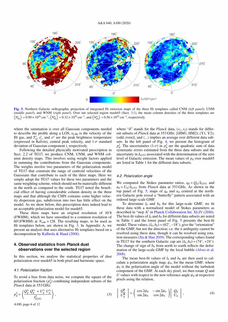
Fig. 3. Northern Galactic orthographic projection of integrated HI emission maps of the three HI templates called CNM (left panel), UNM(middle panel), and WNM (right panel). Over our selected region mask65 (Sect. 3.1), the mean column densities of the three templates are⟨Nc

HI

⟩= 0.90× 1020 cm−2,

⟨Nu

HI

⟩= 0.32× 1020 cm−2, and

⟨Nw

HI

⟩= 0.56× 1020 cm−2, respectively.

where the summation is over all Gaussian components neededto describe the profile along a LOS, vLSR is the velocity of theHI gas, and T i

0, vic, and σi are the peak brightness temperature

(expressed in Kelvin), central peak velocity, and 1σ standarddeviation of Gaussian component i, respectively.

Following the detailed physically motivated prescription inSect. 2.2 of TG17, we produce CNM, UNM, and WNM col-umn density maps. This involves using weight factors appliedin summing the contributions from the Gaussian components.The weights involve two parameters of the polarization modelof TG17 that constrain the range of centroid velocities of theGaussians that contribute to each of the three maps. Here wesimply adopt the TG17 values for these two parameters and thesame weighting scheme, which should not be materially differentin the north as compared to the south. TG17 noted the benefi-cial effect of having considerable column density in the threemaps and that although the CMN contains some higher veloc-ity dispersion gas, subdivision into two has little effect on themodel. As we show below, this prescription does indeed lead toan acceptable polarization model for mask65.

These three maps have an original resolution of 10.′8(FWHM), which we have smoothed to a common resolution of60′(FWHM) at Nside = 128. The resulting maps, to be used asHI templates below, are shown in Fig. 3. In Appendix A, wepresent an analysis that uses alternative HI templates based on adecomposition by Kalberla & Haud (2018).

4. Observed statistics from Planck dustobservations over the selected region

In this section, we analyse the statistical properties of dustpolarization over mask65 in both pixel and harmonic space.

4.1. Polarization fraction

To avoid a bias from data noise, we compute the square of thepolarization fraction (p2

d) combining independent subsets of thePlanck data at 353 GHz:

p2d =

⟨Qs1

d Qs2d + Us1

d Us2d

I2G353

⟩, (3)

where “d” stands for the Planck data, (s1, s2) stands for differ-ent subsets of Planck data at 353 GHz:

{(HM1, HM2); (Y1, Y2);

(odd, even)}, and 〈...〉 implies an average over different data sub-

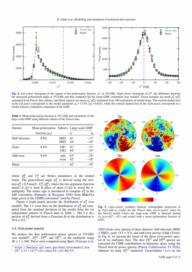
sets. In the left panel of Fig. 4, we present the histogram ofp2

d. The uncertainties (1σ) in p2d are the quadratic sum of data

systematic errors estimated from the three data subsets and theuncertainty in IG353 associated with the determination of the zerolevel of Galactic emission. The mean values of pd over mask65are listed in Table 1 for the different data subsets.

4.2. Polarization angle

We computed the Stokes parameter ratios, qd = Qd/IG353 andud = Ud/IG353 from Planck data at 353 GHz. As shown in thetop panel of Fig. 5, maps of qd and ud centred at the north-ern Galactic pole reveal a “butterfly” pattern associated with anordered large-scale GMF.

To determine l0 and b0 for this large-scale GMF, we fitthese data with a normalised model of Stokes parameters asdescribed in “step A” in Planck Collaboration Int. XLIV (2016).The best-fit values of l0 and b0 for different data subsets are notedin Table 1 and the lower panel of Fig. 5 presents the best-fitmodel. These values, (l0, b0) = (62◦,−18◦), give the “orientation”of the GMF, but not the direction; i.e. the π ambiguity cannot beresolved using these data, though it can be resolved using rota-tion measures (Xu & Han 2019). The corresponding values foundin TG17 for the southern Galactic cap are (l0, b0) = (74◦,+24◦).The change of sign of b0 from north to south reflects the defor-mation of the large-scale GMF by the local bubble (Alves et al.2018).

The mean best-fit values of l0 and b0 are then used to cal-culate a polarization angle map, ψ0, for the mean GMF, whereψ0 is the polarization angle of the model without the turbulentcomponent of the GMF. At each sky pixel, we then rotate Q andU values with respect to the new reference angle ψ0 at respectivepixels using the relation,

[QR

dUR

d

]=

(cos 2ψ0 − sin 2ψ0sin 2ψ0 cos 2ψ0

) [QdUd

], (4)

A100, page 4 of 12

D. Adak et al.: Modelling and simulation of polarized dust emission

0.000 0.015 0.030 0.045

p2

0

2000

4000

6000

8000

Pix

elco

un

ts

Planck data

Model

−90 −60 −30 0 30 60 90

ψR [deg]

0

800

1600

2400

3200

4000

Pix

elco

un

ts

Planck data

Model

Fig. 4. Left panel: histogram of the square of the polarization fraction, p2, at 353 GHz. Right panel: histogram of ψR, the difference betweenthe measured polarization angle at 353 GHz and that computed for the mean GMF orientation over mask65. Green triangles are mean p2

d (ψRd )

estimated from Planck data subsets, and black squares are mean p2m (ψR

m) estimated from 100 realisations of model maps. The vertical dashed linein the left panel corresponds to the model parameter p0 = 15.5% (p2

0 = 0.024), while the vertical dashed line in the right panel corresponds to amodel without a turbulent component of the GMF.

Table 1. Mean polarization fraction at 353 GHz and orientation of thelarge-scale GMF using different subsets of the Planck data.

Dataset Mean polarization Subsets Large-scale GMF

fraction (pd) l0 b0

Half missions 8.8% HM1 61◦ −17◦HM2 64◦ −19◦

Years 8.8% YR1 61◦ −17◦YR2 64◦ −19◦

Odd-even 8.8% odd 63◦ −18◦even 62◦ −18◦

Mean – – 62◦ −18◦

where QRd and UR

d are Stokes parameters in the rotatedframe. The polarization angle ψR

d is derived using the rela-tion ψR

d = 0.5 atan2(−URd ,Q

Rd ), where the two-argument function

atan2(−U,Q) is used in place of atan(−U/Q) to avoid the π-ambiguity. The minus sign is introduced to compute ψR

d in theIAU convention (Hamaker & Bregman 1996) from HEALPixmaps given in the COSMO convention4 used by Planck.

Figure 4 (right panel) presents the distribution of ψRd over

mask65. The 1σ error bars on the distribution of ψRd are com-

puted from the standard deviation of the results from the sixindependent subsets of Planck data in Table 1. The 1σ dis-persion of ψR

d derived from a Gaussian fit to the distribution is16.◦6 ± 0.◦2.

4.3. Dust power spectra

We analyse the dust polarization power spectra at 353 GHzover mask655, DEE

` , DBB` , and DT E

` , in the multipole range40 ≤ ` ≤ 160. These were computed using Xpol (Tristram et al.

4 https://healpix.jpl.nasa.gov/html/intronode12.htm5 DXX

` ≡ `(` + 1)CXX` /(2π), where XX = EE, BB,T E.

-0.1 0.1

135o

45o 315o

225o

60 o

30 o

135o

45o

0o

315o

225o

60 o

30 o

135o

90o

45o

0o

315o

225o

60 o

30 o

135o

90o

45o 315o

225o

60 o

30 o

270o

270o

qd ud

qm um

Fig. 5. Upper panel: northern Galactic orthographic projection ofqd (left) and ud (right) for the Planck data. Lower panel: same forthe best-fit model where the large-scale GMF is directed toward(l0, b0) = (62◦,−18◦) and scaled with a mean polarization fraction of8.8%.

2005) from cross spectra of three datasets: half-missions (HM1× HM2), years (Y1 × Y2), and odd-even surveys (Odd×Even).In Fig. 6, we present the mean of the three cross-power spec-tra in six multipole bins. The dust DEE

` and DBB` spectra are

corrected for CMB contributions in harmonic space using thePlanck best-fit power spectra (Planck Collaboration VI 2020),whereas we keep DT E

` unaltered. Uncertainties (1σ) on the

A100, page 5 of 12

A&A 640, A100 (2020)

40 60 80 100 120 160Multipole `

10

20

50

100

200

D `[µ

K2]

TE

EE

BB

Planck data

40 60 80 100 120 160Multipole `

10

20

50

100

200

M`

[µK

2]

TE

EE

BB

Model

Fig. 6. Left panel: dust EE, BB, and T E cross-power spectra computed from the subsets of Planck data at 353 GHz over mask65. Dashed linesrepresent the best-fit power laws. Right panel: similar plots as left panel computed from 100 realisations of the dust model maps. Error bars are 1σuncertainties as explained in the main text. The filled areas represent the Planck dust power spectra measurements over mask65.

Table 2. Fitted dust power spectra of the Planck data at 353 GHz and ofthe dust model over mask65.

Parameter Planck 353 GHz data Dust model

αEE −2.34 ± 0.16 −2.56 ± 0.18αBB −2.51 ± 0.21 −2.56 ± 0.25αT E −2.43 ± 0.38 −2.75 ± 0.16

χ2EE(Nd.o.f. = 4) 2.2 1.3χ2

BB(Nd.o.f. = 4) 1.8 1.3χ2

T E(Nd.o.f. = 4) 2.3 8.3

AEE [µK2CMB] 39.1 ± 2.2 39.9 ± 2.7

ABB [µK2CMB] 22.5 ± 1.6 22.0 ± 1.4

AT E [µK2CMB] 74.2 ± 10.9 65.6 ± 4.0

〈ABB/AEE〉 0.58 ± 0.05 0.57 ± 0.06〈AT E/AEE〉 1.90 ± 0.30 1.85 ± 0.17

binned dust power spectra are the quadratic sum of statisticalnoise computed by Xpol analytically, and systematic uncertain-ties computed from the standard deviation from the three Planckdata subsets.

We also checked the CMB correction at the map level. Wesubtracted the half-mission and odd-even component-separatedCMB SMICA and SEVEM maps (Planck Collaboration IV 2020)from the total Planck maps and then computed cross-powerspectra using these four subsets of the maps. Subtraction ofCMB does not introduce any noticeable changes in the dustpolarization power spectra.

Binned dust power spectra are well described by a power-law model, DXX

` = AXX(`/80)αXX+2, where AXX is the best-fitamplitude at `= 80, αXX is the best-fit spectral index, and againXX = {EE, BB,T E} (Planck Collaboration Int. XXX 2016). Thebest-fit values of AXX and αXX and the respective values of χ2 arelisted in the middle column of Table 2.

The ratio of BB to EE power is about 0.6 over mask65, con-sistent with the E–B asymmetry result of Planck CollaborationInt. XXX (2016). We detect a significant positive T E correlationover mask65, as in TG17 for the southern Galactic cap.

5. Multiphase model of polarized dust emission

We use the modelling framework from TG17, which is basedon a decomposition of HI emission-line data and incorporatesthe phenomenological magnetic field model described in PlanckCollaboration Int. XLIV (2016). We briefly describe the salientconcepts.

We use the fact that dust emission and NHI are correlated sothat templates of NHI can be used as proxies for spatially variabledust intensity. For optically thin dust emission, the model Stokesparameters Im, Qm, and Um at 353 GHz can be written as

Im(n̂) =

N∑i = 1

[1 − p0

(cos2 γi(n̂) −

23

)]ε353 Ni

HI(n̂)

Qm(n̂) =

N∑i = 1

p0 cos2 γi(n̂) cos 2ψi(n̂) ε353 NiHI(n̂) (5)

Um(n̂) = −

N∑i = 1

p0 cos2 γi(n̂) sin 2ψi(n̂) ε353 NiHI(n̂) ,

where N is the number of distinct templates , n̂ is the directionvector, p0 is a parameter related to the dust grain properties (Lee& Draine 1985; Draine & Fraisse 2009; Planck Collaboration Int.XX 2015), γ is the angle made by the local magnetic field withthe plane of the sky, ψ is the polarization angle measured coun-terclockwise from Galactic north6, ε353 is the dust emissivity at353 GHz for each HI template, and NHI is the column densitywithin the particular template. In this work, N = 3, which is rep-resented by the three distinct templates for CNM, UNM, andWNM (Sect. 3.2). This is a remarkably small number to describethe ISM. However, our focus is on demonstrating what essen-tials can nevertheless be captured by a polarization model thatis inherently minimalist and not dependent on fine-tuning. Forsimplicity, ε353 is assumed to be the same for all three templates.

The connection between the dust polarization and the struc-ture of the GMF via the angles γ and ψ is developed as in

6 IAU convention, the minus sign producing U in the COSMO conven-tion.

A100, page 6 of 12

D. Adak et al.: Modelling and simulation of polarized dust emission

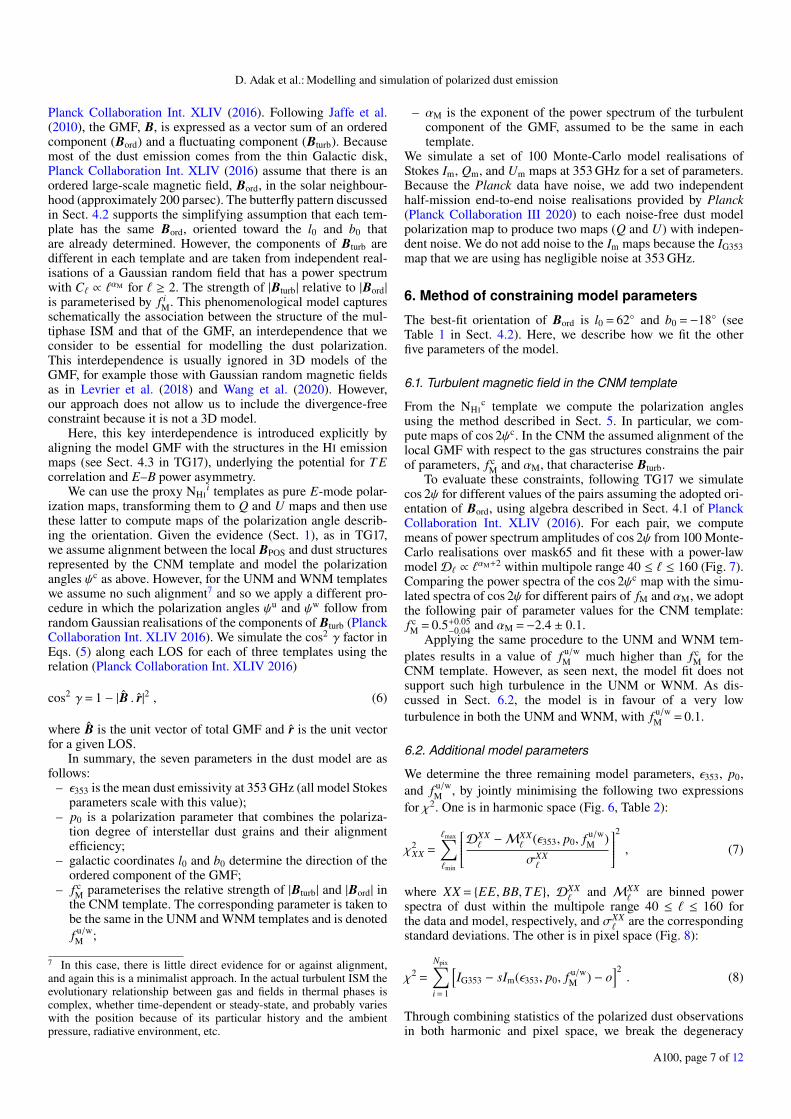
Planck Collaboration Int. XLIV (2016). Following Jaffe et al.(2010), the GMF, B, is expressed as a vector sum of an orderedcomponent (Bord) and a fluctuating component (Bturb). Becausemost of the dust emission comes from the thin Galactic disk,Planck Collaboration Int. XLIV (2016) assume that there is anordered large-scale magnetic field, Bord, in the solar neighbour-hood (approximately 200 parsec). The butterfly pattern discussedin Sect. 4.2 supports the simplifying assumption that each tem-plate has the same Bord, oriented toward the l0 and b0 thatare already determined. However, the components of Bturb aredifferent in each template and are taken from independent real-isations of a Gaussian random field that has a power spectrumwith C` ∝ `

αM for ` ≥ 2. The strength of |Bturb| relative to |Bord|

is parameterised by f iM. This phenomenological model captures

schematically the association between the structure of the mul-tiphase ISM and that of the GMF, an interdependence that weconsider to be essential for modelling the dust polarization.This interdependence is usually ignored in 3D models of theGMF, for example those with Gaussian random magnetic fieldsas in Levrier et al. (2018) and Wang et al. (2020). However,our approach does not allow us to include the divergence-freeconstraint because it is not a 3D model.

Here, this key interdependence is introduced explicitly byaligning the model GMF with the structures in the HI emissionmaps (see Sect. 4.3 in TG17), underlying the potential for T Ecorrelation and E–B power asymmetry.

We can use the proxy NHIi templates as pure E-mode polar-

ization maps, transforming them to Q and U maps and then usethese latter to compute maps of the polarization angle describ-ing the orientation. Given the evidence (Sect. 1), as in TG17,we assume alignment between the local BPOS and dust structuresrepresented by the CNM template and model the polarizationangles ψc as above. However, for the UNM and WNM templateswe assume no such alignment7 and so we apply a different pro-cedure in which the polarization angles ψu and ψw follow fromrandom Gaussian realisations of the components of Bturb (PlanckCollaboration Int. XLIV 2016). We simulate the cos2 γ factor inEqs. (5) along each LOS for each of three templates using therelation (Planck Collaboration Int. XLIV 2016)

cos2 γ= 1 − |B̂ . r̂|2 , (6)

where B̂ is the unit vector of total GMF and r̂ is the unit vectorfor a given LOS.

In summary, the seven parameters in the dust model are asfollows:

– ε353 is the mean dust emissivity at 353 GHz (all model Stokesparameters scale with this value);

– p0 is a polarization parameter that combines the polariza-tion degree of interstellar dust grains and their alignmentefficiency;

– galactic coordinates l0 and b0 determine the direction of theordered component of the GMF;

– f cM parameterises the relative strength of |Bturb| and |Bord| in

the CNM template. The corresponding parameter is taken tobe the same in the UNM and WNM templates and is denotedf u/wM ;

7 In this case, there is little direct evidence for or against alignment,and again this is a minimalist approach. In the actual turbulent ISM theevolutionary relationship between gas and fields in thermal phases iscomplex, whether time-dependent or steady-state, and probably varieswith the position because of its particular history and the ambientpressure, radiative environment, etc.

– αM is the exponent of the power spectrum of the turbulentcomponent of the GMF, assumed to be the same in eachtemplate.

We simulate a set of 100 Monte-Carlo model realisations ofStokes Im, Qm, and Um maps at 353 GHz for a set of parameters.Because the Planck data have noise, we add two independenthalf-mission end-to-end noise realisations provided by Planck(Planck Collaboration III 2020) to each noise-free dust modelpolarization map to produce two maps (Q and U) with indepen-dent noise. We do not add noise to the Im maps because the IG353map that we are using has negligible noise at 353 GHz.

6. Method of constraining model parameters

The best-fit orientation of Bord is l0 = 62◦ and b0 =−18◦ (seeTable 1 in Sect. 4.2). Here, we describe how we fit the otherfive parameters of the model.

6.1. Turbulent magnetic field in the CNM template

From the NHIc template we compute the polarization angles

using the method described in Sect. 5. In particular, we com-pute maps of cos 2ψc. In the CNM the assumed alignment of thelocal GMF with respect to the gas structures constrains the pairof parameters, f c

M and αM, that characterise Bturb.To evaluate these constraints, following TG17 we simulate

cos 2ψ for different values of the pairs assuming the adopted ori-entation of Bord, using algebra described in Sect. 4.1 of PlanckCollaboration Int. XLIV (2016). For each pair, we computemeans of power spectrum amplitudes of cos 2ψ from 100 Monte-Carlo realisations over mask65 and fit these with a power-lawmodelD` ∝ `

αM+2 within multipole range 40 ≤ ` ≤ 160 (Fig. 7).Comparing the power spectra of the cos 2ψc map with the simu-lated spectra of cos 2ψ for different pairs of fM and αM, we adoptthe following pair of parameter values for the CNM template:f cM = 0.5+0.05

−0.04 and αM =−2.4 ± 0.1.Applying the same procedure to the UNM and WNM tem-

plates results in a value of f u/wM much higher than f c

M for theCNM template. However, as seen next, the model fit does notsupport such high turbulence in the UNM or WNM. As dis-cussed in Sect. 6.2, the model is in favour of a very lowturbulence in both the UNM and WNM, with f u/w

M = 0.1.

6.2. Additional model parameters

We determine the three remaining model parameters, ε353, p0,and f u/w

M , by jointly minimising the following two expressionsfor χ2. One is in harmonic space (Fig. 6, Table 2):

χ2XX =

`max∑`min

DXX` −M

XX` (ε353, p0, f u/w

M )

σXX`

2

, (7)

where XX = {EE, BB,T E}, DXX` and MXX

` are binned powerspectra of dust within the multipole range 40 ≤ ` ≤ 160 forthe data and model, respectively, and σXX

` are the correspondingstandard deviations. The other is in pixel space (Fig. 8):

χ2 =

Npix∑i = 1

[IG353 − sIm(ε353, p0, f u/w

M ) − o]2. (8)

Through combining statistics of the polarized dust observationsin both harmonic and pixel space, we break the degeneracy

A100, page 7 of 12

A&A 640, A100 (2020)

40 60 80 100 120 160Multipole `

10−3

10−2

10−1

D `(cos

2ψ)

fM = 0.4, αM = −2.4

fM = 0.5, αM = −2.4

fM = 0.5, αM = −2.3

fM = 0.5, αM = −2.2

CNM template

Fig. 7. Means of power spectrum amplitudes from simulated modelmaps of cos 2ψ within the multipole range 40 ≤ ` ≤ 160 for differentvalues of fM and αM and the best-fit power laws (dashed lines). Theerror bars (1σ) are standard deviations computed from 100 realisations.Black circles are power spectrum amplitudes from the map of cos 2ψc

computed from the CNM template.

between the two model parameters ε353 and p0 in Eq. (5). Theχ2 of the T−T correlation between IG353 and Im is minimised inpixel space over mask65. To match the observed dust amplitudeat 353 GHz, the value of s should be close to 1 and is kept so byadjusting ε353 during the iterative solution of the two equations.

The best-fit values are ε353 = 146 µKCMB(1020 cm−2)−1,p0 = 15.5%, and f u/w

M = 0.1. Compared to the values of ε353 andp0 found by TG17 in their analysis of the southern Galactic cap,our values differ by factors of 1.2 and 0.84, respectively.

7. Comparison of the model with Planckobservations

Using the methods detailed in Sect. 6, we determined parametersof the Stokes dust model such that several statistical propertiescomputed from the model match the Planck dust observationsat 353 GHz over mask65 in both pixel and harmonic space. Thequality of these matches to constraining the Planck polarizationdata is demonstrated below. Furthermore, we show in Sect. 8that the dust model is able to reproduce the observed inverserelationship between the polarization angle dispersion and thepolarization fraction over mask65, even though these statisticswere not used in determining the model parameters.

7.1. Polarization fraction

We compute the mean square of the polarization fraction, p2m,

from 100 realisations using Eq. (5). The error bars on the meanhistogram are the standard deviations estimated over the 100realisations. As shown in Fig. 4 (left), our model reproducesthe statistical distribution of p2

d quite accurately, including thenegative values of p2

d and the largest values beyond p20.

7.2. Polarization angle

We compute the polarization angle, ψRm, from 100 realisations

of the model, following the method described in Sect. 4.2 and

).

The polarization angle

0 100 200 300 400 500 600 700

IG353[µK]

0

100

200

300

400

500

600

700

I m[µ

K]

Fig. 8. Correlation plot between Im and IG353 at 353 GHz. The blackdashed line is the result of the joint optimisation of Eqs. (7) and (8).

used for the data. For each sky realisation i, we fit the orderedcomponent of GMF using li0 and bi

0 and from the map of themean polarization angle of the GMF ψi

0. At each sky pixel in therealisation of the Stokes model maps we then rotate Qi and Uiwith respect to the new reference angle ψi

0 at respective pixelsusing Eq. (4). The polarization angle ψR

i is then derived fromthe rotated Qi and Ui maps. The mean polarization angle, ψR

m,for the model is computed by taking the mean of the histogramsof ψR

i distributions for each bin. Similarly, the uncertainties foreach bin of the histogram are computed from the standard devi-ation of 100 realisations. As shown in Fig. 4 (right), our modelreproduces the statistical distribution of ψR

d . The dispersion ofψR

m derived from a Gaussian fit is 17.◦5 ± 0.◦4, which is slightlyhigher than that for the data ψR

d : 16.◦6± 0.◦2. The difference mightcome from the fact that the model is not fitted to the Planckdata at ` < 40, which cannot be accomplished accurately overthe limited area of mask65.

7.3. Dust polarization spectra

We compute mean cross-power spectra from 100 sets of twoindependent realisations of the Stokes model maps. We fit thebinned power spectra with power laws: MXX

` = AXX(`/80)αXX+2

within the multipole range 40 ≤ ` ≤ 160. Error bars in eachbin are the standard deviations computed from 100 realisations.Best-fit amplitudes, AXX and exponents, αXX along with the cor-responding χ2 values, are listed in the right column of Table 2.We compare the results with the Planck dust power spectra inFig. 6. The DEE

` and DBB` amplitudes and their ratio match

the values from the data accurately. The DT E` amplitude for the

dust model is slightly lower, but consistent with the Planck datawithin its uncertainty.

7.4. Total intensity

Figure 8 shows the tight correlation between Im and IG353at 353 GHz, which demonstrates that statistically, the modeldust intensity reproduces the observed Planck dust intensity.The best-fit dashed line shown has slope s = 1.0 and offseto =−35 µKCMB, again within the uncertainty of the zero levelin the intensity, 40 µKCMB (Sect. 2.1).

A100, page 8 of 12

D. Adak et al.: Modelling and simulation of polarized dust emission

8. Inverse relationship between the polarizationangle dispersion and the polarization fraction

The polarization angle dispersion function, S, was introducedin Planck Collaboration Int. XIX (2015) to quantify the localdispersion of the dust polarization angle for a given angularresolution and lag δ. An inverse relationship between S andpMAS was found, where pMAS is the modified asymptotic estima-tor of the polarization fraction (Plaszczynski et al. 2014). Thatanalysis was done over 42% of the sky at low and intermedi-ate Galactic latitudes at a resolution of 1◦ (FWHM) with a lagδ= 30′. Planck Collaboration XII (2020) extended this work overthe full sky using GNILC processed intensity and polarizationmaps at a resolution of 160′ (FWHM) with δ= 80′and found thatS ∝ p−1

MAS.Here, we study the relationship between S and pMAS over

mask65 using 353 GHz maps at a resolution of 80′ (FWHM)with δ= 40′. The noise bias parameter needed for pMAS (Montieret al. 2015a,b) is estimated from the smoothed noise covari-ance matrices, σII , σIQ, σIU , σQQ, σQU , σUU at a resolution of80′ (FWHM) and Nside = 128.

In the top panel of Fig. 9, we present the two-dimensionaljoint distribution ofS and pMAS for the Planck data over mask65.The running mean of S in each bin of pMAS follows an inverserelationship, S= (0.◦43 ± 0.◦04)/pMAS. In the bottom panel ofFig. 9, we show the corresponding S–pMAS distribution forour model. This too has an inverse relationship and the slope0.◦50 ± 0.◦05 is very close to that for the Planck data. This isremarkable given that this statistical property of dust polarizationhas not been exploited in the fit of our model parameters.

9. Summary and discussion

In this paper, we analyse the statistical properties of the Planckdust polarization maps at 353 GHz at a 60′ resolution (FWHM)over a low-column-density region that accounts for 65% of thenorthern Galactic cap at latitudes larger than 30◦ (mask65). Wemake use of the multiphase dust polarization model describedin TG17. The model shows how the dust polarization acrossthe sky can be approximated on the basis of proxy HI data: inparticular, three independent templates notionally representingthe contributions from the CNM, UNM, and WNM. The modelhas seven adjustable parameters whose values are determined byreproducing Planck observations at 353 GHz: in particular, theone-point statistics of p and ψ in pixel space, and the EE, BB,and T E power spectra in harmonic space. Our main results canbe summarised as follows.

– The butterfly pattern seen in qd and ud maps (Fig. 5) aroundthe pole is associated with an ordered GMF, which wefind has a mean orientation in Galactic coordinates toward(l0, b0) = (62◦,−18◦) (Sect. 4.2). The best-fit value of l0is roughly consistent with the earlier values derived fromstarlight polarization (Ellis & Axon 1978; Heiles 1996).

– From the Planck data, we find a BB/EE power ratio of0.58 and significant positive T E correlation over mask65(Sect. 4.3). The key property in our model that allows themodel to reproduce these observations (Sect. 7.3) is thealignment of the local magnetic field BPOS and the HIstructure in the CNM template (Sect. 5).

– The observed distributions of p and ψ over mask65 show ascatter that is comparable to that of the distributions reportedfor the whole sky in Planck Collaboration XII (2020).Our model successfully reproduced these one-point statis-tics associated with LOS depolarization (Sects. 7.1 and 7.2)

10−1 100 101

pMAS[%]

100

101

S[deg

]

S × pMAS = 0.43◦ ± 0.04◦

0.0

0.2

0.4

0.6

0.8

1.0

1.2

1.4

log

( cou

nts)

10−1 100 101

pMAS[%]

100

101

S[deg

]

S × pMAS = 0.50◦ ± 0.05◦

0.0

0.2

0.4

0.6

0.8

1.0

1.2

1.4

log

( cou

nts)

σ

–

–

Fig. 9. Top panel: two-dimensional histogram of the joint distributionof S and pMAS over mask65 for the Planck data at a resolution of 80′with lag δ= 40′. The black circles show the mean of S in bins of pMAScontaining the same number of map pixels. Error bars are the standarddeviation of S in each bin. The black dotted line is a fit of the runningmean. Bottom panel: same as top panel, but for the model.

by introducing fluctuations in the GMF orientation that areuncorrelated between the three independent HI templates(Sect. 3.2).

– The best-fit value of the parameter, p0, that measures thegrain alignment efficiency combined with the intrinsic polar-ization fraction of interstellar dust emission at 353 GHz,is 15.5%. The best-fit value of the dust emissivity isε353 = 146 µKCMB(1020 cm−2)−1 (Sect. 6.2).

– To match the observed EE, BB, and T E amplitudes, themodel fit yields a low value of the parameter f u/w

M speci-fying the relative amplitude of the turbulent component ofthe GMF in the UNM and WNM. This value, 0.1, is sig-nificantly smaller than the value f c

M = 0.5 characterising theCNM (Sect. 6.1).

– The spectral index of the turbulent component of the GMF,αM =−2.4, fitted over mask65 (Sect. 6.1), is consistent withthe value reported in TG17. These two complementary

A100, page 9 of 12

A&A 640, A100 (2020)

analyses reveal that the spectral index of turbulent mag-netic field closely matches the power-law index of dustpolarization power spectra, as expected.

– Our model also reproduces the inverse relationship betweenthe polarization angle dispersion, S, and the polarizationfraction, pMAS, present in the Planck data, despite the factthat we do not utilise this phenomenon in fitting the modelparameters (Sect. 8). Our work reinforces the conclusion inPlanck Collaboration XII (2020) that the inverse relationshipof S and pMAS is a generic feature associated with the GMFstructure.

This work demonstrates that the phenomenological model intro-duced in TG17 for the southern Galactic cap also works wellin the northern hemisphere. The next step in our modellingwork will be to extend this framework to multiple frequenciesby incorporating spectral energy distributions for the dust emis-sion associated with the three HI templates thus introducingthe potential for frequency decorrelation of the dust polariza-tion. This is a necessary step towards investigating the utility ofthis framework for evaluating component separation methods forfuture CMB missions.

Acknowledgements. We gratefully acknowledge the use of the Aquila cluster atNISER, Bhubaneswar. D.A. acknowledges the University Grants CommissionIndia for providing financial support as Senior Research Fellow. This work wassupported by the Science and Engineering Research Board, Department of Sci-ence and Technology, Govt. of India grant number SERB/ECR/2018/000826 andthe Natural Sciences and Engineering Research Council of Canada. Some of theresults in this paper have been derived using the HEALPix package. The PlanckLegacy Archive (PLA) contains all public products originating from the Planckmission, and we take the opportunity to thank ESA/Planck and the Planck Col-laboration for the same. This work has made use of HI data of the EBHIS surveyheaded by the Argelander-Institut für Astronomie (PI: J. Kerp) in collaborationwith the Max-Planck-Institut für Radioastronomie and funded by the DeutscheForschungsgemeinschaft (grants KE757/7-1 to 7-3). The Gaussian decomposi-tion of the EBHIS data was supported by the Estonian Research Council grantIUT26-2, and by the European Regional Development Fund (TK133).

ReferencesAlves, M. I. R., Boulanger, F., Ferrière, K., & Montier, L. 2018, A&A, 611, L5Andersson, B. G., Lazarian, A., & Vaillancourt, J. E. 2015, ARA&A, 53, 501Arendt, R. G., Odegard, N., Weiland, J. L., et al. 1998, ApJ, 508, 74Ashton, P. C., Ade, P. A. R., Angilè, F. E., et al. 2018, ApJ, 857, 10Caldwell, R. R., Hirata, C., & Kamionkowski, M. 2017, ApJ, 839, 91Clark, S. E. 2018, ApJ, 857, L10Clark, S. E., & Hensley, B. S. 2019, ApJ, 887, 136Clark, S. E., Peek, J. E. G., & Putman, M. E. 2014, ApJ, 789, 82Clark, S. E., Hill, J. C., Peek, J. E. G., Putman, M. E., & Babler, B. L. 2015,

Phys. Rev. Lett., 115, 241302Clark, S. E., Peek, J. E. G., & Miville-Deschênes, M. A. 2019, ApJ, 874, 171Davis, Jr. L., & Greenstein, J. L. 1951, ApJ, 114, 206Draine, B. T., & Fraisse, A. A. 2009, ApJ, 696, 1Ellis, R. S., & Axon, D. J. 1978, Ap&SS, 54, 425Fabbri, R., & Pollock, M. 1983, Phys. Lett. B, 125, 445Ghosh, T., Boulanger, F., Martin, P. G., et al. 2017, A&A, 601, A71Gillmon, K., Shull, J. M., Tumlinson, J., & Danforth, C. 2006, ApJ, 636, 891Górski, K. M., Hivon, E., Banday, A. J., et al. 2005, ApJ, 622, 759

Hamaker, J. P., & Bregman, J. D. 1996, A&AS, 117, 161Haud, U. 2000, A&A, 364, 83Haud, U. 2013, A&A, 552, A108Heiles, C. 1996, ApJ, 462, 316HI4PI Collaboration (Ben Bekhti, N., et al.) 2016, A&A, 594, A116Hivon, E., Górski, K. M., Netterfield, C. B., et al. 2002, ApJ, 567, 2Jaffe, T. R., Leahy, J. P., Banday, A. J., et al. 2010, MNRAS, 401, 1013Jow, D. L., Hill, R., Scott, D., et al. 2018, MNRAS, 474, 1018Kalberla, P. M. W., & Haud, U. 2018, A&A, 619, A58Kalberla, P. M. W., Kerp, J., Haud, U., et al. 2016, ApJ, 821, 117Kandel, D., Lazarian, A., & Pogosyan, D. 2017, MNRAS, 472, L10Kandel, D., Lazarian, A., & Pogosyan, D. 2018, MNRAS, 478, 530Kerp, J., Winkel, B., Ben Bekhti, N., Flöer, L., & Kalberla, P. M. W. 2011, Astron.

Nachr., 332, 637Lazarian, A. 2007, J. Quant. Spectr. Rad. Transf., 106, 225Lee, H. M., & Draine, B. T. 1985, ApJ, 290, 211Levrier, F., Neveu, J., Falgarone, E., et al. 2018, A&A, 614, A124Martin, P. G. 2007, EAS Publ. Ser., 23, 165Martin, P. G., Blagrave, K. P. M., Lockman, F. J., et al. 2015, ApJ, 809, 153Montier, L., Plaszczynski, S., Levrier, F., et al. 2015a, A&A, 574, A135Montier, L., Plaszczynski, S., Levrier, F., et al. 2015b, A&A, 574, A136Planck Collaboration XXIV. 2011, A&A, 536, A24Planck Collaboration XI. 2014, A&A, 571, A11Planck Collaboration I. 2016, A&A, 594, A1Planck Collaboration I. 2020, A&A, in press, https://doi.org/10.1051/0004-6361/201833880

Planck Collaboration III. 2020, A&A, in press, https://doi.org/10.1051/0004-6361/201832909

Planck Collaboration IV. 2020, A&A, in press, https://doi.org/10.1051/0004-6361/201833881

Planck Collaboration VI. 2020, A&A, in press, https://doi.org/10.1051/0004-6361/201833910

Planck Collaboration XI. 2020, A&A, in press, https://doi.org/10.1051/0004-6361/201832618

Planck Collaboration XII. 2020, A&A, in press, https://doi.org/10.1051/0004-6361/201833885

Planck Collaboration Int. XVII. 2014, A&A, 566, A55Planck Collaboration Int. XIX. 2015, A&A, 576, A104Planck Collaboration Int. XX. 2015, A&A, 576, A105Planck Collaboration Int. XXII. 2015, A&A, 576, A107Planck Collaboration Int. XXX. 2016, A&A, 586, A133Planck Collaboration Int. XXXII. 2016, A&A, 586, A135Planck Collaboration Int. XXXV. 2016, A&A, 586, A138Planck Collaboration Int. XXXVIII. 2016, A&A, 586, A141Planck Collaboration Int. XLIV. 2016, A&A, 596, A105Plaszczynski, S., Montier, L., Levrier, F., & Tristram, M. 2014, MNRAS, 439,

4048Remazeilles, M., Dickinson, C., Eriksen, H. K. K., & Wehus, I. K. 2016,

MNRAS, 458, 2032Savage, B. D., Bohlin, R. C., Drake, J. F., & Budich, W. 1977, ApJ, 216, 291Soler, J. D., Hennebelle, P., Martin, P. G., et al. 2013, ApJ, 774, 128Soler, J. D., Ade, P. A. R., Angilè, F. E., et al. 2017, A&A, 603, A64Starobinskij, A. A. 1979, Pisma v Zhurnal Eksperimentalnoi i Teoreticheskoi

Fiziki, 30, 719Stein, W. 1966, ApJ, 144, 318Tristram, M., Macías-Pérez, J. F., Renault, C., & Santos, D. 2005, MNRAS, 358,

833Vaillancourt, J. E., & Matthews, B. C. 2012, ApJS, 201, 13Wang, J., Jaffe, T. R., Ensslin, T. A., et al. 2020, ApJS, 247, 18Wilson, T. L., Rohlfs, K., & Hüttemeister, S. 2009, Tools of Radio Astronomy

(Springer-Verlag, Berlin)Winkel, B., Kerp, J., Flöer, L., et al. 2016, A&A, 585, A41Xu, J., & Han, J. L. 2019, MNRAS, 486, 4275

A100, page 10 of 12

D. Adak et al.: Modelling and simulation of polarized dust emission

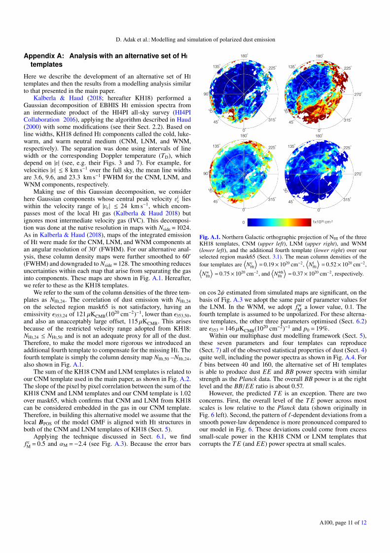
Appendix A: Analysis with an alternative set of HI

templates

Here we describe the development of an alternative set of HItemplates and then the results from a modelling analysis similarto that presented in the main paper.

Kalberla & Haud (2018; hereafter KH18) performed aGaussian decomposition of EBHIS HI emission spectra froman intermediate product of the HI4PI all-sky survey (HI4PICollaboration 2016), applying the algorithm described in Haud(2000) with some modifications (see their Sect. 2.2). Based online widths, KH18 defined HI components called the cold, luke-warm, and warm neutral medium (CNM, LNM, and WNM,respectively). The separation was done using intervals of linewidth or the corresponding Doppler temperature (TD), whichdepend on |v| (see, e.g. their Figs. 3 and 7). For example, forvelocities |v| ≤ 8 km s−1 over the full sky, the mean line widthsare 3.6, 9.6, and 23.3 km s−1 FWHM for the CNM, LNM, andWNM components, respectively.

Making use of this Gaussian decomposition, we considerhere Gaussian components whose central peak velocity vi

c lieswithin the velocity range of |vc| ≤ 24 km s−1, which encom-passes most of the local HI gas (Kalberla & Haud 2018) butignores most intermediate velocity gas (IVC). This decomposi-tion was done at the native resolution in maps with Nside = 1024.As in Kalberla & Haud (2018), maps of the integrated emissionof HI were made for the CNM, LNM, and WNM components atan angular resolution of 30′ (FWHM). For our alternative anal-ysis, these column density maps were further smoothed to 60′(FWHM) and downgraded to Nside = 128. The smoothing reducesuncertainties within each map that arise from separating the gasinto components. These maps are shown in Fig. A.1. Hereafter,we refer to these as the KH18 templates.

We refer to the sum of the column densities of the three tem-plates as NHI,24. The correlation of dust emission with NHI,24on the selected region mask65 is not satisfactory, having anemissivity ε353,24 of 121 µKCMB(1020 cm−2)−1, lower than ε353,50,and also an unacceptably large offset, 115 µKCMB. This arisesbecause of the restricted velocity range adopted from KH18:NHI,24 ≤ NHI,50 and is not an adequate proxy for all of the dust.Therefore, to make the model more rigorous we introduced anadditional fourth template to compensate for the missing HI. Thefourth template is simply the column density map NHI,50 –NHI,24,also shown in Fig. A.1.

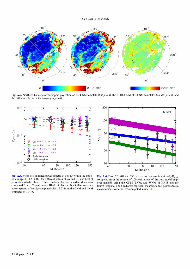
The sum of the KH18 CNM and LNM templates is related toour CNM template used in the main paper, as shown in Fig. A.2.The slope of the pixel by pixel correlation between the sum of theKH18 CNM and LNM templates and our CNM template is 1.02over mask65, which confirms that CNM and LNM from KH18can be considered embedded in the gas in our CNM template.Therefore, in building this alternative model we assume that thelocal BPOS of the model GMF is aligned with HI structures inboth of the CNM and LNM templates of KH18 (Sect. 5).

Applying the technique discussed in Sect. 6.1, we findf cM = 0.5 and αM =−2.4 (see Fig. A.3). Because the error bars

0 1x1020 cm-2

180o

135o

45o

0o

315o

225o

60 o

30 o

180o

135o

45o

0o

315o

225o

60 o

30 o

180o

135o

90o

45o

0o

315o

225o

60 o

30 o

180o

135o

90o

45o

0o

315o

225o

60 o

30 o270o

270o

Fig. A.1. Northern Galactic orthographic projection of NHI of the threeKH18 templates, CNM (upper left), LNM (upper right), and WNM(lower left), and the additional fourth template (lower right) over ourselected region mask65 (Sect. 3.1). The mean column densities of thefour templates are

⟨Nc

HI

⟩= 0.19× 1020 cm−2,

⟨N l

HI

⟩= 0.52× 1020 cm−2,⟨

NwHI

⟩= 0.75× 1020 cm−2, and

⟨N4th

HI

⟩= 0.37× 1020 cm−2, respectively.

on cos 2ψ estimated from simulated maps are significant, on thebasis of Fig. A.3 we adopt the same pair of parameter values forthe LNM. In the WNM, we adopt f w

M a lower value, 0.1. Thefourth template is assumed to be unpolarized. For these alterna-tive templates, the other three parameters optimised (Sect. 6.2)are ε353 = 146 µKCMB(1020 cm−2)−1 and p0 = 19%.

Within our multiphase dust modelling framework (Sect. 5),these seven parameters and four templates can reproduce(Sect. 7) all of the observed statistical properties of dust (Sect. 4)quite well, including the power spectra as shown in Fig. A.4. For` bins between 40 and 160, the alternative set of HI templatesis able to produce dust EE and BB power spectra with similarstrength as the Planck data. The overall BB power is at the rightlevel and the BB/EE ratio is about 0.57.

However, the predicted T E is an exception. There are twoconcerns. First, the overall level of the T E power across mostscales is low relative to the Planck data (shown originally inFig. 6 left). Second, the pattern of `-dependent deviations from asmooth power-law dependence is more pronounced compared toour model in Fig. 6. These deviations could come from excesssmall-scale power in the KH18 CNM or LNM templates thatcorrupts the T E (and EE) power spectra at small scales.

A100, page 11 of 12

A&A 640, A100 (2020)

0 2x1020 cm-2

180o

135o

90o

45o

0o

315o

225o

60 o

30 o

180o

135o

45o

0o

315o

225o

60 o

30 o

180o

135o

45o

0o

315o

225o

60 o

30 o

270o

-2 2x1020 cm-2

Fig. A.2. Northern Galactic orthographic projection of our CNM template (left panel), the KH18 CNM plus LNM templates (middle panel), andthe difference between the two (right panel).

40 60 80 100 120 160Multipole `

10−3

10−2

10−1

D `(cos

2ψ

)

fM = 0.4, αM = −2.4

fM = 0.5, αM = −2.4

fM = 0.5, αM = −2.3

fM = 0.5, αM = −2.2

CNM template

LNM template

40 60 80 100 120 160Multipole `

10

20

50

100

200

M`

[µK

2]

TE

EE

BB

Model

Fig. A.3. Mean of simulated power spectra of cos 2ψ within the multi-pole range 40 ≤ ` ≤ 160 for different values of fM and αM and best fitpower-law (dashed lines). The error-bars (1σ) are standard deviationscomputed from 100 realisations.Black circles and black diamonds arepower spectra of cos 2ψ computed (Sect. 3.2) from the CNM and LNMtemplates of KH18.

40 60 80 100 120 160Multipole `

10−3

10−2

10−1

D `(cos

2ψ

)

fM = 0.4, αM = −2.4

fM = 0.5, αM = −2.4

fM = 0.5, αM = −2.3

fM = 0.5, αM = −2.2

CNM template

LNM template

40 60 80 100 120 160Multipole `

10

20

50

100

200

M`

[µK

2]

TE

EE

BB

Model

Fig. A.4. Dust EE, BB, and T E cross-power spectra in units of µK2CMB

computed from the subsets of 100 realisations of the dust model mapsover mask65 using the CNM, LNM, and WNM of KH18 and thefourth template. The filled areas represent the Planck dust power spectrameasurements over mask65 computed in Sect. 4.3.

A100, page 12 of 12