Embed Size (px)
Citation preview
HAL Id: inria-00567546https://hal.inria.fr/inria-00567546
Submitted on 21 Feb 2011
HAL is a multi-disciplinary open accessarchive for the deposit and dissemination of sci-entific research documents, whether they are pub-lished or not. The documents may come fromteaching and research institutions in France orabroad, or from public or private research centers.
L’archive ouverte pluridisciplinaire HAL, estdestinée au dépôt et à la diffusion de documentsscientifiques de niveau recherche, publiés ou non,émanant des établissements d’enseignement et derecherche français ou étrangers, des laboratoirespublics ou privés.
DVB-T2 Simulation Model for OPNETAdlen Ksentini, Yassine Hadjadj-Aoul
To cite this version:Adlen Ksentini, Yassine Hadjadj-Aoul. DVB-T2 Simulation Model for OPNET. [Research Report] PI1967, 2011, pp.17. �inria-00567546�
Publications Internes de l’IRISAISSN : 2102-6327PI 1967 – Fevrier 2011
DVB-T2 Simulation Model for OPNET
Adlen Ksentini * , Yassine Hadjadj-Aoul ** ,[email protected], [email protected]
Abstract: DVB-T2 is offering a new way for broadcasting value-added services to end users, such as High Definition(HD) TV and 3D TV. Thanks to the advances made in digital signal processing, and specifically in channel coding, DVB-T2 brings an increased transfer capacity of 50% and a new flexibility in services’ broadcasting in contrast with the firstgeneration DVB-T standard. As DVB-T2 is still in deployment’s test, simulation model could be an interesting way toevaluate the performance of this network in supporting new value-added services. In this paper, we describe the new featuresand enhancements we have integrated within the DVB-T2 module in OPNET, and in particular: (i) a realistic physicalmodel;(ii) an MPEG-TS layer with an IP encapsulator;(iii) hierarchical application layer ables to use pcap traces to simulatereal video traces. Also, we include an extensive simulation campaign in order to well understand the performance of DVB-T2networks.
Key-words: DVB-T2, Simulation, OPNET, Performance Evaluation
Modele de simulation des reseaux DVB-T2 pour OPNET
Resume : DVB-T2 est entrain de devenir le nouveau standard de diffusion de services a forte valeur rajoutee, tel quela television haute definition ou la television en 3D. Capable d’adresser les stations fixes et mobiles ce qui est largementfavorise par l’augmentation des debits physiques, ou on atteint un gain de 50% par rapport au standard precedent DVB-T.Du fait que le DVB-T2 est en cours de test et de deploiement, il est necessaire de disposer d’un modele de simulation pourevaluer les performances de ces reseaux et leurs capacite a supporter ces nouveaux services. Dans cet article, nous decrivonsles nouvelles fonctionnalites ainsi que les ameliorations effectuees pour integrer un modele de simulation dans OPNET, etparticulierement : (i) une couche physique realistique;(ii) la couche MPEG-TS avec un encapsulateur IP; (iii) une coucheapplication capable de lire des traces pcap pour simuler des flux video. De plus, nous presentons une etude detaillee desresultats de simulations pour diffrents scenarios, fixe et mobile.
Mots cles : DVB-T2, Simulation, OPNET, evaluation de performances
This work is supported by the FUI’9 SVC4QoE project* Projet Dionysos : equipe commune INRIA, CNRS, ENS, INSA et universite de Rennes 1
** Projet Dionysos : equipe commune INRIA, CNRS, ENS, INSA et universite de Rennes 1
c©IRISA – Campus de Beaulieu – 35042 Rennes Cedex – France – +33 2 99 84 71 00 – www.irisa.fr
2 A. Ksentini & Y. Hadjadj
1 Introduction
DVB-T2 [1] is the second generation standard for digital terrestrial television broadcasting. Thanks to the advances madein digital signal processing, and specifically in channel coding, DVB-T2 brings an increased transfer capacity of 50% and anew flexibility in services’ broadcasting when compared to the first generation DVB-T standard published in 1997.
To allow a high robustness against multipath propagation, DVB-T2 uses a Coded Orthogonal Frequency Division Mul-tiplexing (COFDM) multi-carrier modulation, in a similar way to DVB-T. A wider range of schemes is proposed, from 1Kcarrier up to 32K carrier, to meet the requirements of a wide range of receiving situations (fixed and mobile) and networktopologies (single and multiple frequency networks). In terms of channel coding, DVB-T2 uses Low Density Parity Check(LDPC) block codes and Bose-Chaudhui-Hochquenghene (BCH) coding, which provide more robust error correction than theconvolutional and Reed Solomon encoding used in DVB-T. Most of the capacity gain of DVB-T2 comes from this fundamentalchange of channel coding.
The DVB-T2 physical layer data channel is divided into logical entities called the Physical Layer Pipes (PLP). EachPLP carries one logical data stream. Examples of such a logical data stream, would be an audio-visual multimedia streamalong with the associated signaling information, or an hierarchical application streams, which can address at the same timedifferent qualities as it is the case for Scalable Video Coding (SVC) [2]. The PLP architecture is designated to be flexibleso that arbitrary adjustments of robustness and capacity can be easily done. Thus, using different PLP enable broadcastingof multiple services or groups of services with separate channel coding and modulation settings on a single radio channel.Broadcasting several service components over the same channel is thus made possible, with differentiated levels of robustness,which was not possible with the previous DVB-T standard. Regarding the upper layers, the DVB-T2 provides two mainIP encapsulation protocols, the MPEG-TS [3], packetization, which has been the classical encapsulation scheme for DVBservices, and the Generic Stream Encapsulation (GSE) [4], which was designated to provide appropriate encapsulation forIP traffic.
Simulation tools, meanwhile, are a good mean to evaluate the performance of a system in different conditions. This is alsouseful to dimension a system and optimize its performance, which represent an interesting issues, particularly for DVB-T2network as it is still in test. OPNET [5], on the other hand, is one of the leading network simulators that provides powerfulsimulation capability for testing networks architectures and protocols. Reader can refer to [6], for an interesting comparisonof several computer simulations, with a brief focus on OPNET.In this work, we describe the features and enhancements we added to support DVB-T2 simulation in OPNET. The mostimportant features we introduced are: (1) a realistic physical layer that uses measured Bit Error Rate (BER) versus Signal-to-Noise Ratio (SNR) traces for different modulation schemes; (2) MPEG-TS layer, with an IP encapsulator based on Uni-directional Lightweight Encapsulation (ULE) [7]; (3) an application layer that supports hierarchical streams, and associateseach stream with a PLP. Also, the developed application layer is able to parse pcap traces to simulate real video traffics. Thepurpose of this simulation model is to enable the evaluation, in a realistic environment, the capacity of DVB-T2 to supportnew services, such as High Definition video broadcast, for both fixed and mobile receivers. To the best of our knowledge thisis the first simulator platform for DVB-T2 networks. Further, this DVB-T2 simulation model could be extended easily tosimulate DVB-H, which shares many features with DVB-T2 (only the physical layer that needs modification).
This paper is organized as follow: section 2 presents the details of the developed DVB-T2 chain in OPNET. In section 3,we show simulation results obtained for the fix and the mobiles scenarios. We conclude this paper in section 4.
2 DVB-T2 OPNET Model
2.1 Model Overview
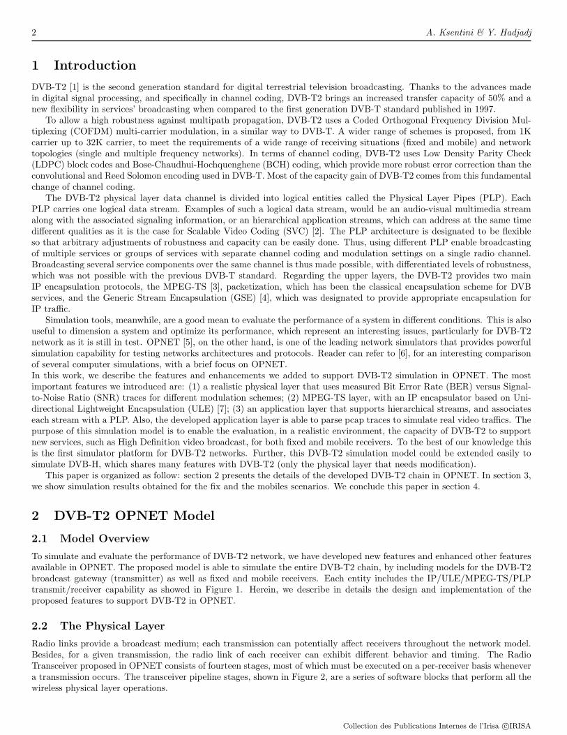
To simulate and evaluate the performance of DVB-T2 network, we have developed new features and enhanced other featuresavailable in OPNET. The proposed model is able to simulate the entire DVB-T2 chain, by including models for the DVB-T2broadcast gateway (transmitter) as well as fixed and mobile receivers. Each entity includes the IP/ULE/MPEG-TS/PLPtransmit/receiver capability as showed in Figure 1. Herein, we describe in details the design and implementation of theproposed features to support DVB-T2 in OPNET.
2.2 The Physical Layer
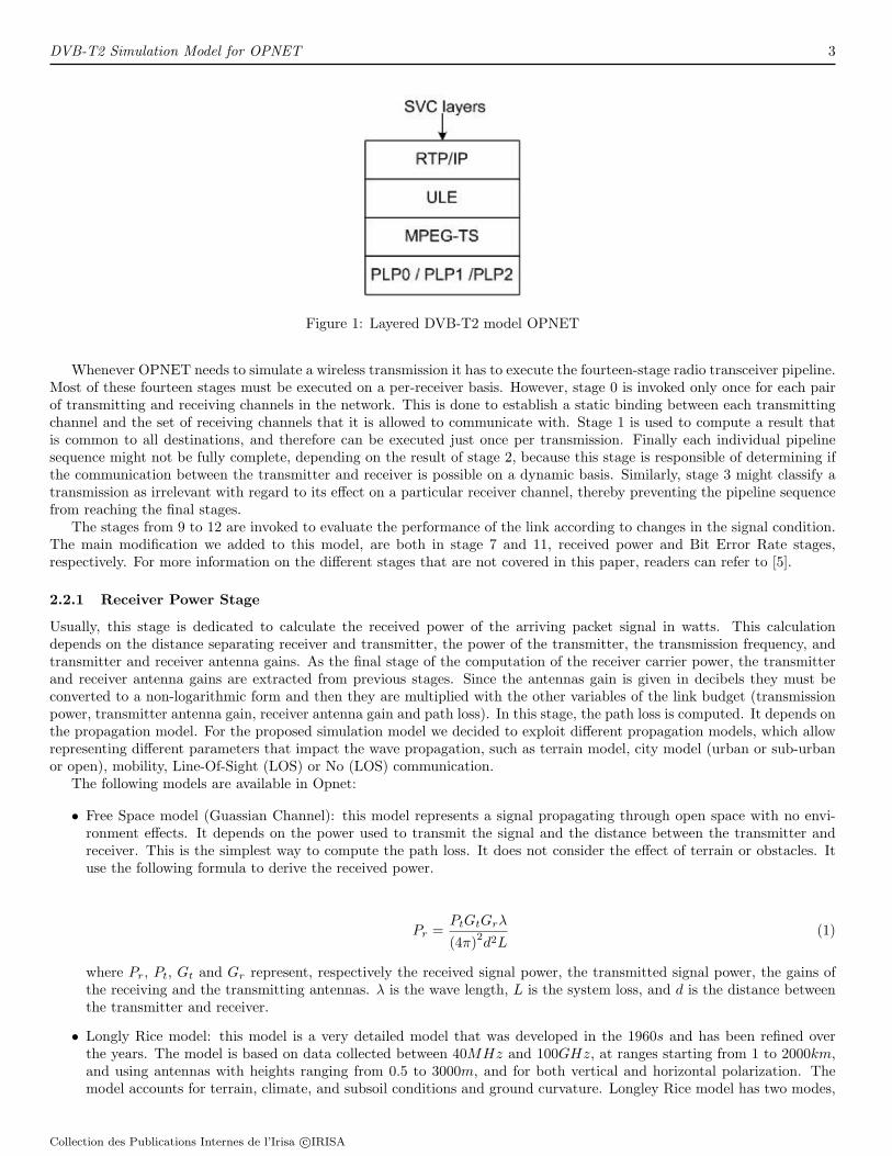
Radio links provide a broadcast medium; each transmission can potentially affect receivers throughout the network model.Besides, for a given transmission, the radio link of each receiver can exhibit different behavior and timing. The RadioTransceiver proposed in OPNET consists of fourteen stages, most of which must be executed on a per-receiver basis whenevera transmission occurs. The transceiver pipeline stages, shown in Figure 2, are a series of software blocks that perform all thewireless physical layer operations.
Collection des Publications Internes de l’Irisa c©IRISA
DVB-T2 Simulation Model for OPNET 3
Figure 1: Layered DVB-T2 model OPNET
Whenever OPNET needs to simulate a wireless transmission it has to execute the fourteen-stage radio transceiver pipeline.Most of these fourteen stages must be executed on a per-receiver basis. However, stage 0 is invoked only once for each pairof transmitting and receiving channels in the network. This is done to establish a static binding between each transmittingchannel and the set of receiving channels that it is allowed to communicate with. Stage 1 is used to compute a result thatis common to all destinations, and therefore can be executed just once per transmission. Finally each individual pipelinesequence might not be fully complete, depending on the result of stage 2, because this stage is responsible of determining ifthe communication between the transmitter and receiver is possible on a dynamic basis. Similarly, stage 3 might classify atransmission as irrelevant with regard to its effect on a particular receiver channel, thereby preventing the pipeline sequencefrom reaching the final stages.
The stages from 9 to 12 are invoked to evaluate the performance of the link according to changes in the signal condition.The main modification we added to this model, are both in stage 7 and 11, received power and Bit Error Rate stages,respectively. For more information on the different stages that are not covered in this paper, readers can refer to [5].
2.2.1 Receiver Power Stage
Usually, this stage is dedicated to calculate the received power of the arriving packet signal in watts. This calculationdepends on the distance separating receiver and transmitter, the power of the transmitter, the transmission frequency, andtransmitter and receiver antenna gains. As the final stage of the computation of the receiver carrier power, the transmitterand receiver antenna gains are extracted from previous stages. Since the antennas gain is given in decibels they must beconverted to a non-logarithmic form and then they are multiplied with the other variables of the link budget (transmissionpower, transmitter antenna gain, receiver antenna gain and path loss). In this stage, the path loss is computed. It depends onthe propagation model. For the proposed simulation model we decided to exploit different propagation models, which allowrepresenting different parameters that impact the wave propagation, such as terrain model, city model (urban or sub-urbanor open), mobility, Line-Of-Sight (LOS) or No (LOS) communication.
The following models are available in Opnet:
• Free Space model (Guassian Channel): this model represents a signal propagating through open space with no envi-ronment effects. It depends on the power used to transmit the signal and the distance between the transmitter andreceiver. This is the simplest way to compute the path loss. It does not consider the effect of terrain or obstacles. Ituse the following formula to derive the received power.
Pr =PtGtGrλ
(4π)2d2L(1)
where Pr, Pt, Gt and Gr represent, respectively the received signal power, the transmitted signal power, the gains ofthe receiving and the transmitting antennas. λ is the wave length, L is the system loss, and d is the distance betweenthe transmitter and receiver.
• Longly Rice model: this model is a very detailed model that was developed in the 1960s and has been refined overthe years. The model is based on data collected between 40MHz and 100GHz, at ranges starting from 1 to 2000km,and using antennas with heights ranging from 0.5 to 3000m, and for both vertical and horizontal polarization. Themodel accounts for terrain, climate, and subsoil conditions and ground curvature. Longley Rice model has two modes,
Collection des Publications Internes de l’Irisa c©IRISA
4 A. Ksentini & Y. Hadjadj
Figure 2: The radio Transceiver execution sequence for one transmission
Collection des Publications Internes de l’Irisa c©IRISA

DVB-T2 Simulation Model for OPNET 5
point-to-point and area. The point-to-point mode makes use of detailed terrain data or characteristics to predict thepath loss, whereas the area mode uses general information about the terrain characteristics to predict the path loss.
• HATA model: The Hata model (sometimes called the Okumura Hata model) is an empirical formulation that incor-porates the graphical information from the Okumura model [8]-[9]. For the Hata model, the prediction area is dividedinto terrain categories: open area, suburban area, and urban area. The open area model represents locations with openspace, no tall trees or buildings in the path, and the land cleared for 300m−400m ahead (i.e., farmland). The suburbanarea model represents a village or a highway scattered with trees and houses, some obstacles near the mobile, but notvery congested. The urban area model represents a built-up city or large town with large buildings and houses withtwo or more stories, or larger villages with close houses and tall thickly grown trees. The Hata model uses the urbanarea as a baseline and then applies correction factors for conversion to other classifications. There are three differentformulas for the Hata model: for urban areas, for suburban areas, and for open areas. For instance, the followingformula presents the Urban area:
L50(db) = 69.55 + 26.16log(fc − 13.84log(ht − a(ht) + [44.9− 6.55log(ht)]log(d) (2)
where fc, ht, a(hr) and d represent, respectively, the transmission frequency, the transmitter antenna height, thereceiver antenna height and the distance.
• CIR model: this model (originally published by Comite Consultatif International des Radio communications) is asimplified version of the Hata model. It has one parameter: the Building Percentage, which represents the percentageof area covered by buildings.
In most environments, the path loss is sufficiently variable that it must be characterized statistically. This is particularlytrue for mobile communications where either or both terminals may be moving (changing the relative geometry) and whereboth are using wide-angle or omnidirectional antennas. Multipath models vary depending upon the type of consideredenvironment and the involved frequencies. While detailed databases of most urban areas are available, statistical modelingbased on empirical data (oftentimes fitted to specific empirical data) is still the method of choice. One exception is theplanning of fixed LOS links, which can be facilitated by geometric multipath computations using urban databases. Tothis end, we added the possibility to simulate fading power envelop channel by using Ricean or Rayleigh models. In fact,the probability of various fade depths depend upon the characteristics of the multipath environment. When there are asufficient number of reflections present and they are adequately randomized (in both phase and amplitude), it is possible touse probability theory to analyze the underlying probability density functions (pdf) and thereby determine the probabilitythat a given fade depth will be exceeded. For the NLOS case, where all elements of the received signal are reflections ordiffraction components and no single component is dominant, the analysis draws on the central limit theorem to argue thatthe in-phase and quadrature components of the received signal will be independent, zero-mean Gaussian random variableswith equal variance. In this case, the pdf of the received signal envelope will be a Rayleigh random variable. Using theRayleigh pdf, the analyst can then determine the probability of any given fade depth being exceeded. It is also possible tooptimize the system detection and coding algorithms for Rayleigh fading rather than for Gaussian channel. On the otherhand, if there is an LOS component present or if one of the reflections is dominant, then the envelope of the received signalis characterized by a Ricean pdf, rather than a Rayleigh. The determination of the probability of a fade is a little morecomplicated when the Ricean pdf is used, but it is still tractable.
To obtain more realistic physical layer for DVB-T2, we adapted the Ricean and Rayleigh models presented in [10] forOPNET 10.0 (we use for this simulation OPNET 14.5). In [10] the authors present a simple method of modeling small scaleRicean (or Rayleigh) fading. Small scale fading is caused by movement of the transmitter/receiver, or of other objects inthe environment. This motion can be characterized by the Doppler spreading. Fading can be modeled by using frequency-domain random numbers with appropriate statistics and then applying time-correlation by performing spectral shaping onthese data using the Doppler spread. Note that, a dataset containing the component of time-sequenced fading envelope ispre-computed. The parameters to be adjusted are time-average power P , the maximum Doppler frequency and the Riceank factor. For Rayleigh model k = 0.
2.2.2 Bit Error Rate stage
The purpose of this stage is to derive the probability of bit errors during the interval of the SNR. This is not an actual rateof bit errors, but the expected rate, which is usually based on the SNR and also depends on the type of modulation used forthe transmitted signal.
The process is as follows: the simulator kernel extracts, first, the SNR calculated on stage 10 and adds it to the processinggain to obtain the effective SNR. Then the effective SNR is converted from the log scale and expressed as Eb/N0. Where: Eb
Collection des Publications Internes de l’Irisa c©IRISA
6 A. Ksentini & Y. Hadjadj
Figure 3: 16 QAM BER vs. Eb/N0
Figure 4: Transmitter Model
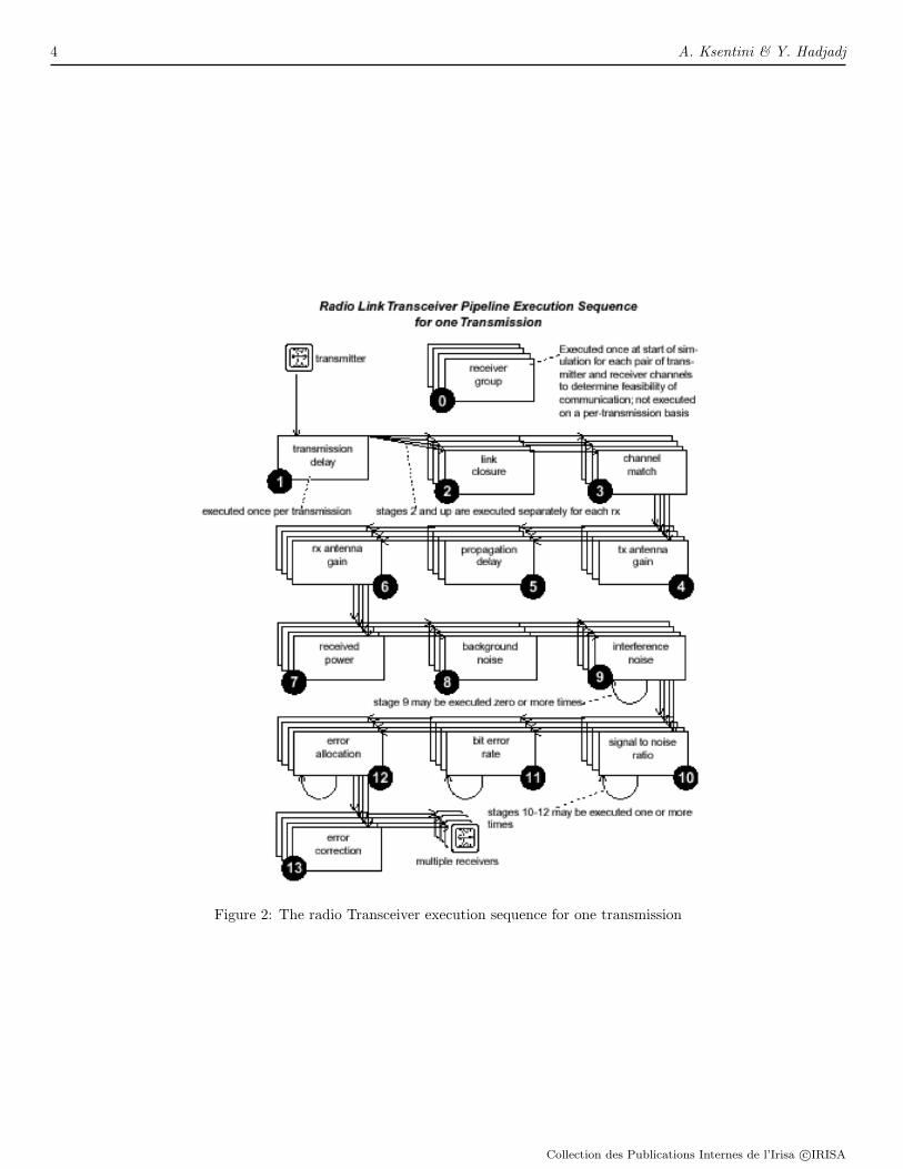
is the received energy per bit (in joules), N0 is the noise power spectral density (in watts/hertz). Then the bit error rate isderived from the effective SNR based on a modulation curve assigned to the receiver. Figure 3 shows the modulation curveswith different FEC protections used in the simulation model for DVB-T2. They are based on real traces obtained througha real DVB-T2 decoder. It represents the BER versus the Eb/N0 for different modulation techniques as well as differentFEC protection. Note that, these values are obtained after low Density Parity Check (LDPC) and before Bose-Chaudhui-Hochquenghene (BCH) correction. From Figure 3 we see clearly that higher is the FEC protection, higher is the robustnessof the physical modulation. For instance, only 3db is necessary to decode the physical signal, in case of 16QAM1/2 (2bitssent for 1bit for FEC). For low protection (16QAM5/6), 6db is necessary to begin to decode the signal.
3 Transmitter Model (DVB-T2 Gateway)
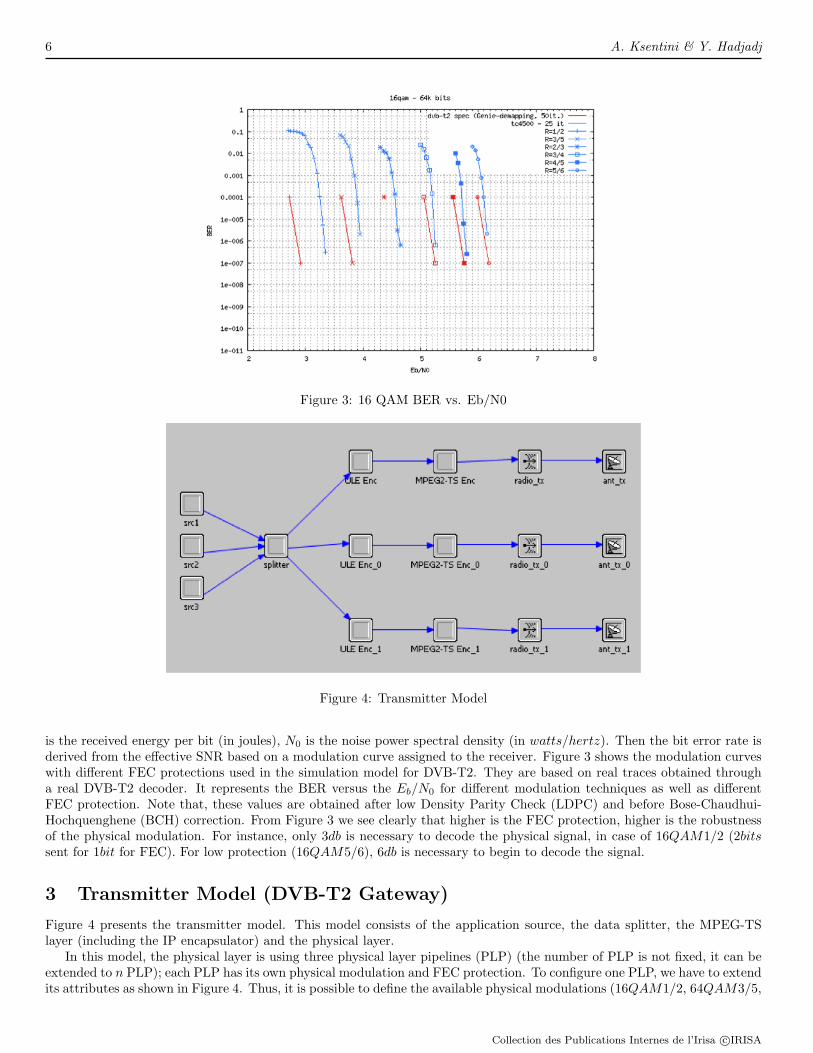
Figure 4 presents the transmitter model. This model consists of the application source, the data splitter, the MPEG-TSlayer (including the IP encapsulator) and the physical layer.
In this model, the physical layer is using three physical layer pipelines (PLP) (the number of PLP is not fixed, it can beextended to n PLP); each PLP has its own physical modulation and FEC protection. To configure one PLP, we have to extendits attributes as shown in Figure 4. Thus, it is possible to define the available physical modulations (16QAM1/2, 64QAM3/5,
Collection des Publications Internes de l’Irisa c©IRISA
DVB-T2 Simulation Model for OPNET 7
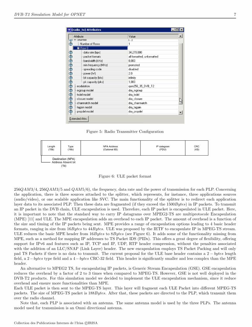
Figure 5: Radio Transmitter Configuration
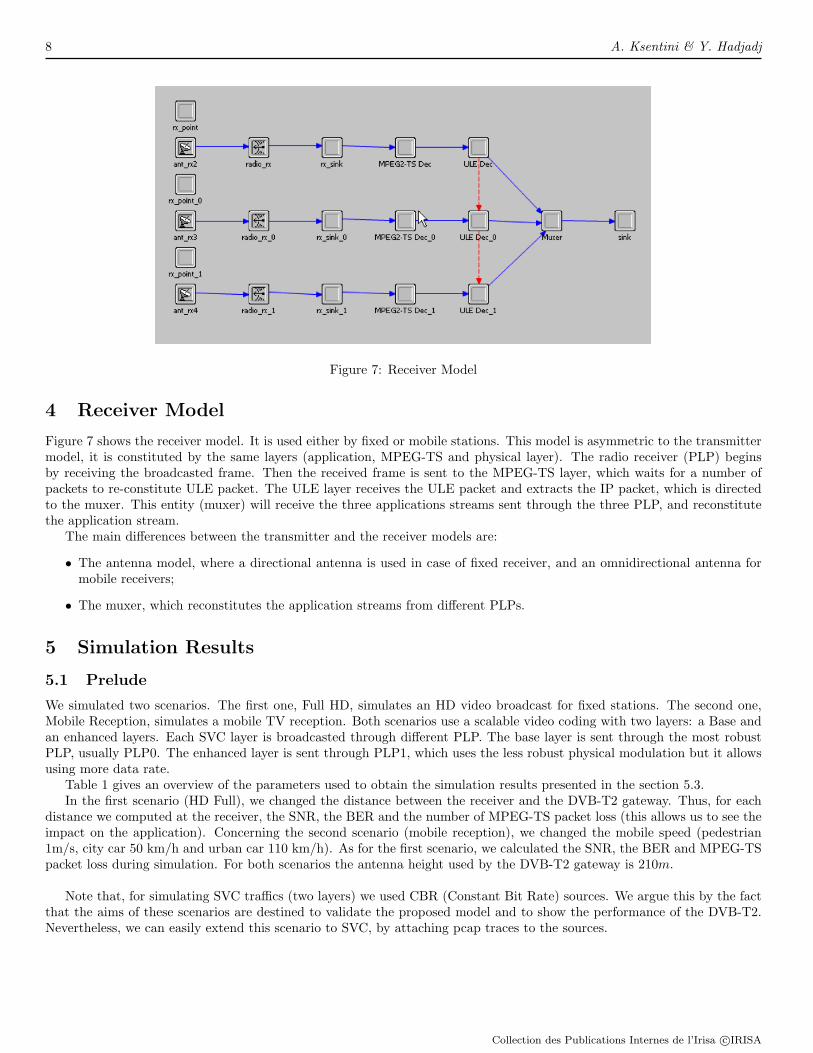
Figure 6: ULE packet format
256QAM3/4, 256QAM3/5 and QAM5/6), the frequency, data rate and the power of transmission for each PLP. Concerningthe application, there is three sources attached to the splitter, which represents, for instance, three applications sources(audio/video), or one scalable application like SVC. The main functionality of the splitter is to redirect each applicationlayer data to its associated PLP. Then these data are fragmented (if they exceed the 1500Bytes) in IP packets. To transmitan IP packet in the DVB chain, ULE encapsulation is used. Therefore, each IP packet is encapsulated in ULE packet. Here,it is important to note that the standard way to carry IP datagrams over MPEG2-TS are multiprotocole Encapsulation(MPE) [11] and ULE. The MPE encapsulation adds an overhead to each IP packet. The amount of overhead is a function ofthe size and timing of the IP packets being sent. MPE provides a range of encapsulation options leading to 4 basic headerformats, ranging in size from 16Bytes to 44Bytes. ULE was proposed by the IETF to encapsulate IP in MPEG-TS stream.ULE reduces the basic MPE header from 16Bytes to 8Bytes (see Figure 6). It adds some of the functionality missing fromMPE, such as a method for mapping IP addresses to TS Packet IDS (PIDs). This offers a great degree of flexibility, offeringsupport for IPv6 and features such as IP, TCP and IP, UDP, RTP header compression, without the penalties associatedwith the addition of an LLC/SNAP (Link Layer) header. The new encapsulation employs TS Packet Packing and will onlypad TS Packets if there is no data to transmit. The current proposal for the ULE base header contains a 2 − bytes lengthfield, a 2− bytes type field and a 4− bytes CRC-32 field. This header is significantly smaller and less complex than the MPEheader.
An alternative to MPEG2 TS, for encapsulating IP packets, is Generic Stream Encapsulation (GSE). GSE encapsulationreduces the overhead by a factor of 2 to 3 times when compared to MPEG-TS. However, GSE is not well deployed in theDVB-T2 products. For this simulation model we decided to implement the ULE encapsulation mechanism, since it reduceoverhead and ensure more functionalities than MPE.Each ULE packet is then sent to the MPEG-TS layer. This layer will fragment each ULE Packet into different MPEG-TSpackets. The size of MPEG-TS packet is 188Bytes. After that, these packets are directed to the PLP, which transmit themover the radio channel.
Note that, each PLP is associated with an antenna. The same antenna model is used by the three PLPs. The antennamodel used for transmission is an Omni directional antenna.
Collection des Publications Internes de l’Irisa c©IRISA
8 A. Ksentini & Y. Hadjadj
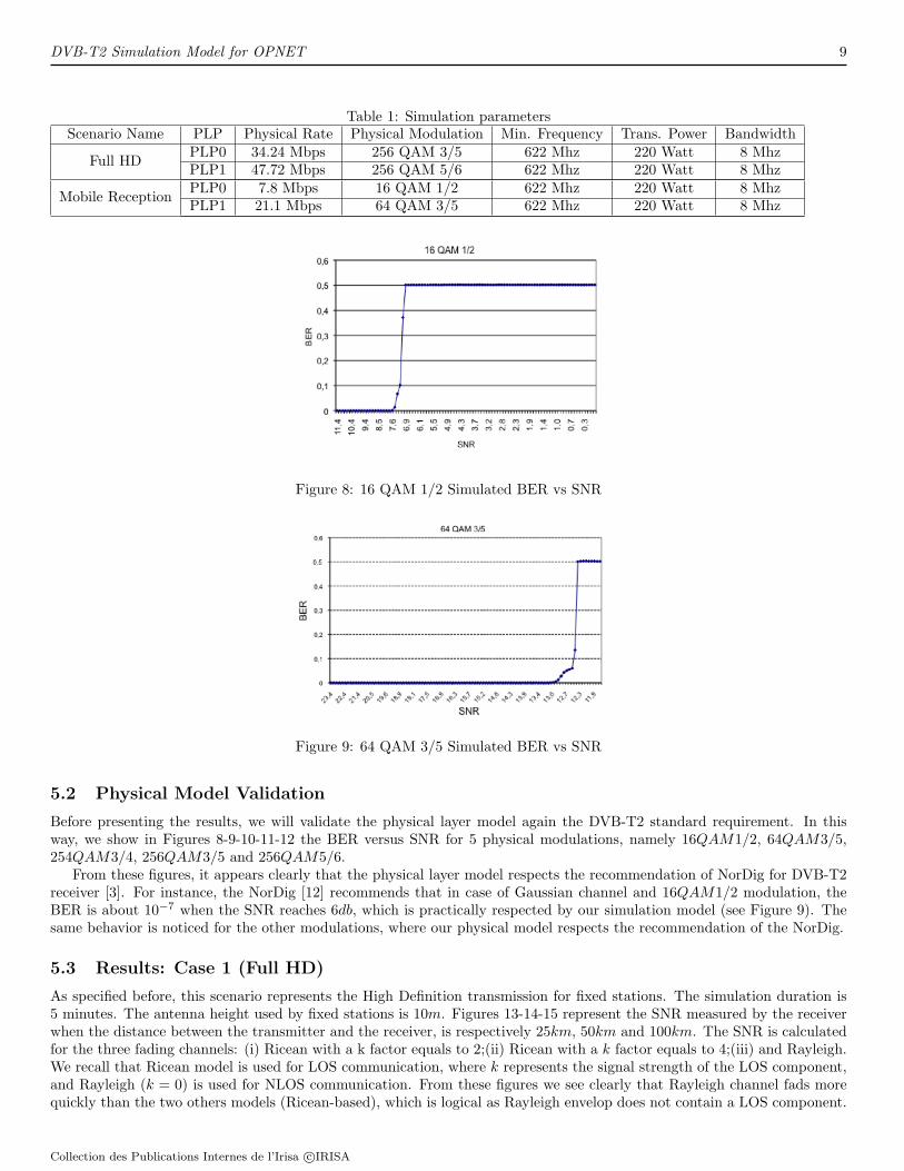
Figure 7: Receiver Model
4 Receiver Model
Figure 7 shows the receiver model. It is used either by fixed or mobile stations. This model is asymmetric to the transmittermodel, it is constituted by the same layers (application, MPEG-TS and physical layer). The radio receiver (PLP) beginsby receiving the broadcasted frame. Then the received frame is sent to the MPEG-TS layer, which waits for a number ofpackets to re-constitute ULE packet. The ULE layer receives the ULE packet and extracts the IP packet, which is directedto the muxer. This entity (muxer) will receive the three applications streams sent through the three PLP, and reconstitutethe application stream.
The main differences between the transmitter and the receiver models are:
• The antenna model, where a directional antenna is used in case of fixed receiver, and an omnidirectional antenna formobile receivers;
• The muxer, which reconstitutes the application streams from different PLPs.
5 Simulation Results
5.1 Prelude
We simulated two scenarios. The first one, Full HD, simulates an HD video broadcast for fixed stations. The second one,Mobile Reception, simulates a mobile TV reception. Both scenarios use a scalable video coding with two layers: a Base andan enhanced layers. Each SVC layer is broadcasted through different PLP. The base layer is sent through the most robustPLP, usually PLP0. The enhanced layer is sent through PLP1, which uses the less robust physical modulation but it allowsusing more data rate.
Table 1 gives an overview of the parameters used to obtain the simulation results presented in the section 5.3.In the first scenario (HD Full), we changed the distance between the receiver and the DVB-T2 gateway. Thus, for each
distance we computed at the receiver, the SNR, the BER and the number of MPEG-TS packet loss (this allows us to see theimpact on the application). Concerning the second scenario (mobile reception), we changed the mobile speed (pedestrian1m/s, city car 50 km/h and urban car 110 km/h). As for the first scenario, we calculated the SNR, the BER and MPEG-TSpacket loss during simulation. For both scenarios the antenna height used by the DVB-T2 gateway is 210m.
Note that, for simulating SVC traffics (two layers) we used CBR (Constant Bit Rate) sources. We argue this by the factthat the aims of these scenarios are destined to validate the proposed model and to show the performance of the DVB-T2.Nevertheless, we can easily extend this scenario to SVC, by attaching pcap traces to the sources.
Collection des Publications Internes de l’Irisa c©IRISA
DVB-T2 Simulation Model for OPNET 9
Table 1: Simulation parametersScenario Name PLP Physical Rate Physical Modulation Min. Frequency Trans. Power Bandwidth
Full HD PLP0 34.24 Mbps 256 QAM 3/5 622 Mhz 220 Watt 8 MhzPLP1 47.72 Mbps 256 QAM 5/6 622 Mhz 220 Watt 8 Mhz
Mobile Reception PLP0 7.8 Mbps 16 QAM 1/2 622 Mhz 220 Watt 8 MhzPLP1 21.1 Mbps 64 QAM 3/5 622 Mhz 220 Watt 8 Mhz
Figure 8: 16 QAM 1/2 Simulated BER vs SNR
Figure 9: 64 QAM 3/5 Simulated BER vs SNR
5.2 Physical Model Validation
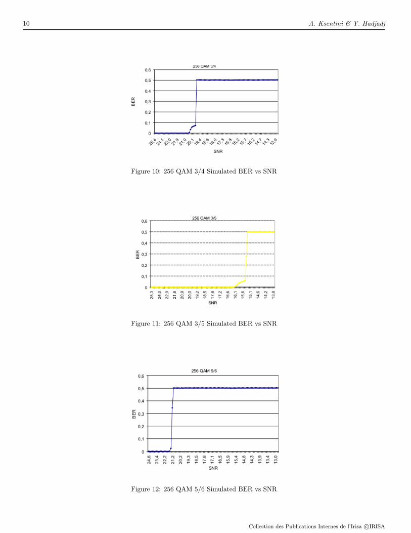
Before presenting the results, we will validate the physical layer model again the DVB-T2 standard requirement. In thisway, we show in Figures 8-9-10-11-12 the BER versus SNR for 5 physical modulations, namely 16QAM1/2, 64QAM3/5,254QAM3/4, 256QAM3/5 and 256QAM5/6.
From these figures, it appears clearly that the physical layer model respects the recommendation of NorDig for DVB-T2receiver [3]. For instance, the NorDig [12] recommends that in case of Gaussian channel and 16QAM1/2 modulation, theBER is about 10−7 when the SNR reaches 6db, which is practically respected by our simulation model (see Figure 9). Thesame behavior is noticed for the other modulations, where our physical model respects the recommendation of the NorDig.
5.3 Results: Case 1 (Full HD)
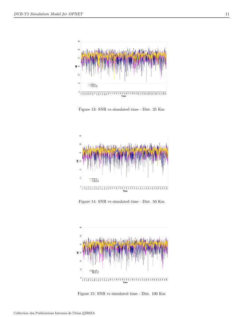
As specified before, this scenario represents the High Definition transmission for fixed stations. The simulation duration is5 minutes. The antenna height used by fixed stations is 10m. Figures 13-14-15 represent the SNR measured by the receiverwhen the distance between the transmitter and the receiver, is respectively 25km, 50km and 100km. The SNR is calculatedfor the three fading channels: (i) Ricean with a k factor equals to 2;(ii) Ricean with a k factor equals to 4;(iii) and Rayleigh.We recall that Ricean model is used for LOS communication, where k represents the signal strength of the LOS component,and Rayleigh (k = 0) is used for NLOS communication. From these figures we see clearly that Rayleigh channel fads morequickly than the two others models (Ricean-based), which is logical as Rayleigh envelop does not contain a LOS component.
Collection des Publications Internes de l’Irisa c©IRISA
10 A. Ksentini & Y. Hadjadj
Figure 10: 256 QAM 3/4 Simulated BER vs SNR
Figure 11: 256 QAM 3/5 Simulated BER vs SNR
Figure 12: 256 QAM 5/6 Simulated BER vs SNR
Collection des Publications Internes de l’Irisa c©IRISA
DVB-T2 Simulation Model for OPNET 11
Figure 13: SNR vs simulated time - Dist. 25 Km
Figure 14: SNR vs simulated time - Dist. 50 Km
Figure 15: SNR vs simulated time - Dist. 100 Km
Collection des Publications Internes de l’Irisa c©IRISA
12 A. Ksentini & Y. Hadjadj
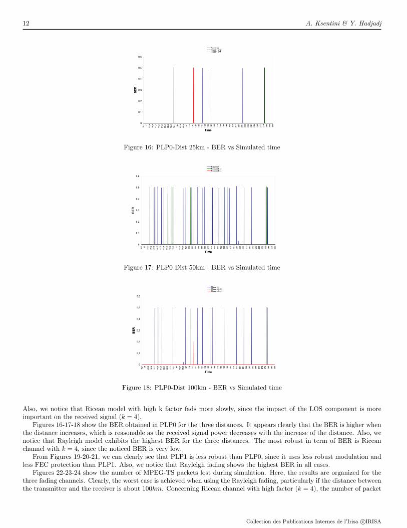
Figure 16: PLP0-Dist 25km - BER vs Simulated time
Figure 17: PLP0-Dist 50km - BER vs Simulated time
Figure 18: PLP0-Dist 100km - BER vs Simulated time
Also, we notice that Ricean model with high k factor fads more slowly, since the impact of the LOS component is moreimportant on the received signal (k = 4).
Figures 16-17-18 show the BER obtained in PLP0 for the three distances. It appears clearly that the BER is higher whenthe distance increases, which is reasonable as the received signal power decreases with the increase of the distance. Also, wenotice that Rayleigh model exhibits the highest BER for the three distances. The most robust in term of BER is Riceanchannel with k = 4, since the noticed BER is very low.
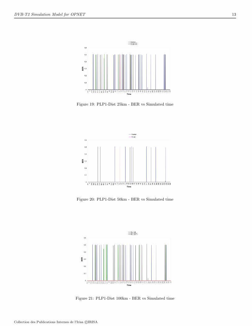
From Figures 19-20-21, we can clearly see that PLP1 is less robust than PLP0, since it uses less robust modulation andless FEC protection than PLP1. Also, we notice that Rayleigh fading shows the highest BER in all cases.
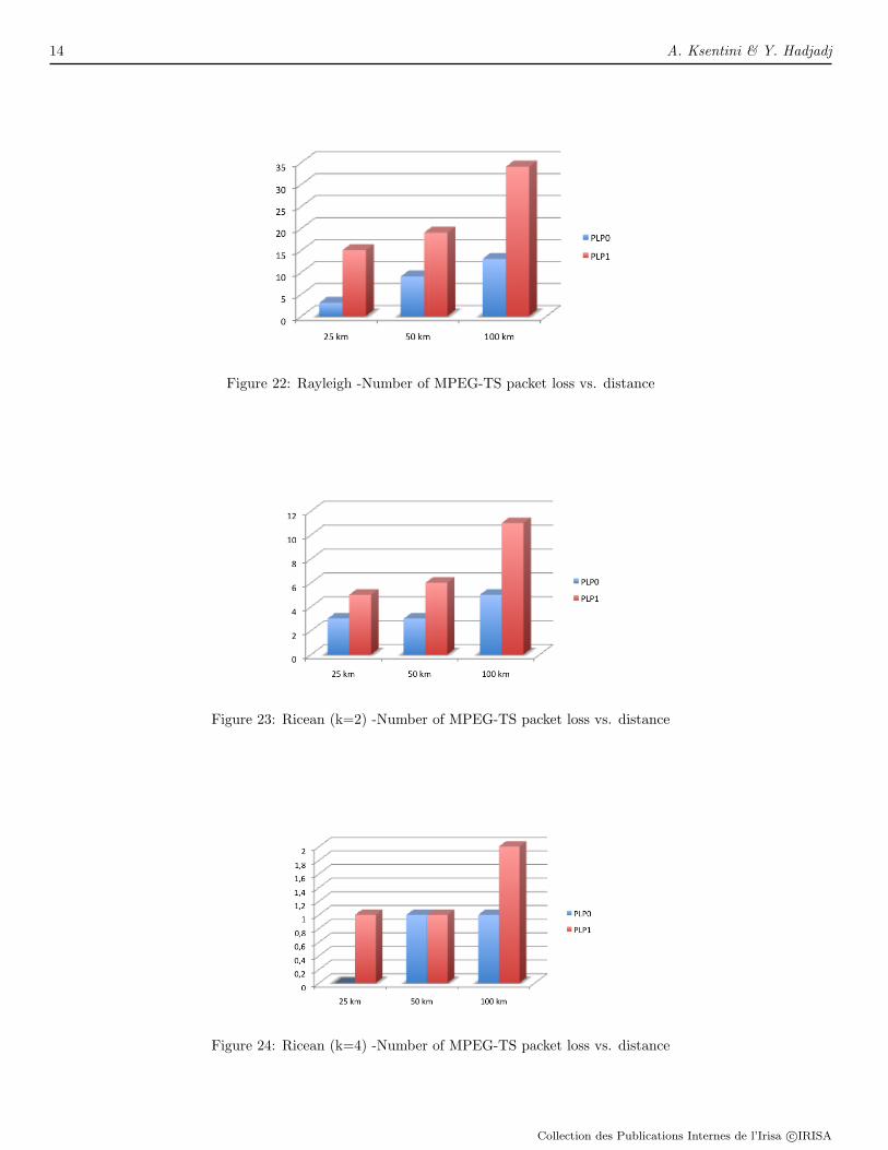
Figures 22-23-24 show the number of MPEG-TS packets lost during simulation. Here, the results are organized for thethree fading channels. Clearly, the worst case is achieved when using the Rayleigh fading, particularly if the distance betweenthe transmitter and the receiver is about 100km. Concerning Ricean channel with high factor (k = 4), the number of packet
Collection des Publications Internes de l’Irisa c©IRISA
DVB-T2 Simulation Model for OPNET 13
Figure 19: PLP1-Dist 25km - BER vs Simulated time
Figure 20: PLP1-Dist 50km - BER vs Simulated time
Figure 21: PLP1-Dist 100km - BER vs Simulated time
Collection des Publications Internes de l’Irisa c©IRISA
14 A. Ksentini & Y. Hadjadj
Figure 22: Rayleigh -Number of MPEG-TS packet loss vs. distance
Figure 23: Ricean (k=2) -Number of MPEG-TS packet loss vs. distance
Figure 24: Ricean (k=4) -Number of MPEG-TS packet loss vs. distance
Collection des Publications Internes de l’Irisa c©IRISA
DVB-T2 Simulation Model for OPNET 15
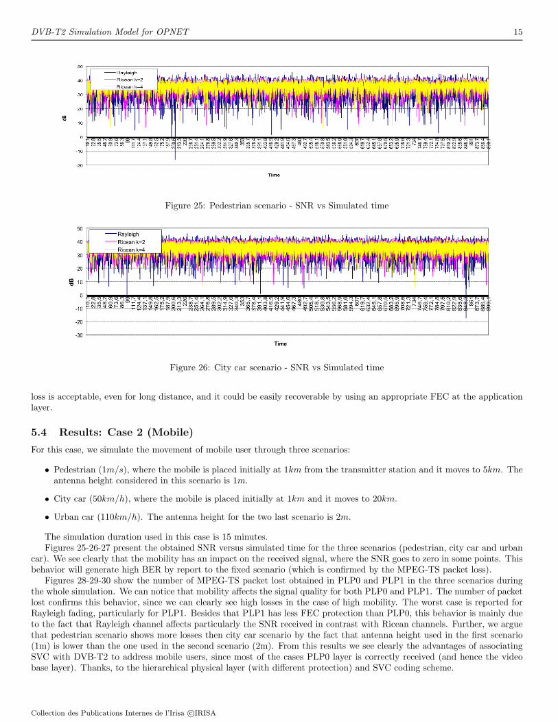
Figure 25: Pedestrian scenario - SNR vs Simulated time
Figure 26: City car scenario - SNR vs Simulated time
loss is acceptable, even for long distance, and it could be easily recoverable by using an appropriate FEC at the applicationlayer.
5.4 Results: Case 2 (Mobile)
For this case, we simulate the movement of mobile user through three scenarios:
• Pedestrian (1m/s), where the mobile is placed initially at 1km from the transmitter station and it moves to 5km. Theantenna height considered in this scenario is 1m.
• City car (50km/h), where the mobile is placed initially at 1km and it moves to 20km.
• Urban car (110km/h). The antenna height for the two last scenario is 2m.
The simulation duration used in this case is 15 minutes.Figures 25-26-27 present the obtained SNR versus simulated time for the three scenarios (pedestrian, city car and urban
car). We see clearly that the mobility has an impact on the received signal, where the SNR goes to zero in some points. Thisbehavior will generate high BER by report to the fixed scenario (which is confirmed by the MPEG-TS packet loss).
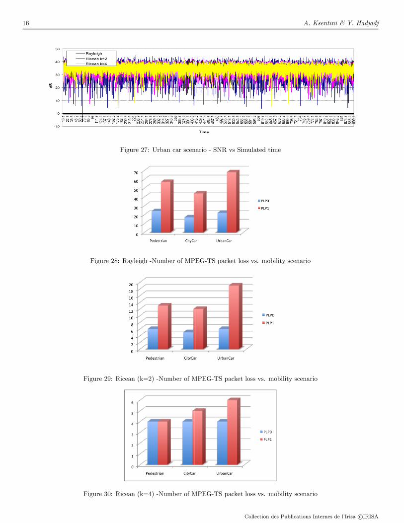
Figures 28-29-30 show the number of MPEG-TS packet lost obtained in PLP0 and PLP1 in the three scenarios duringthe whole simulation. We can notice that mobility affects the signal quality for both PLP0 and PLP1. The number of packetlost confirms this behavior, since we can clearly see high losses in the case of high mobility. The worst case is reported forRayleigh fading, particularly for PLP1. Besides that PLP1 has less FEC protection than PLP0, this behavior is mainly dueto the fact that Rayleigh channel affects particularly the SNR received in contrast with Ricean channels. Further, we arguethat pedestrian scenario shows more losses then city car scenario by the fact that antenna height used in the first scenario(1m) is lower than the one used in the second scenario (2m). From this results we see clearly the advantages of associatingSVC with DVB-T2 to address mobile users, since most of the cases PLP0 layer is correctly received (and hence the videobase layer). Thanks, to the hierarchical physical layer (with different protection) and SVC coding scheme.
Collection des Publications Internes de l’Irisa c©IRISA
16 A. Ksentini & Y. Hadjadj
Figure 27: Urban car scenario - SNR vs Simulated time
Figure 28: Rayleigh -Number of MPEG-TS packet loss vs. mobility scenario
Figure 29: Ricean (k=2) -Number of MPEG-TS packet loss vs. mobility scenario
Figure 30: Ricean (k=4) -Number of MPEG-TS packet loss vs. mobility scenario
Collection des Publications Internes de l’Irisa c©IRISA
DVB-T2 Simulation Model for OPNET 17
6 Conclusion
This paper presents design and implementation of new features to support DVB-T2 simulation in OPNET. The proposedfeatures includes realistic physical channel mode, MPEG-TS layer with an IP encapsulator based on ULE, and a hierarchicalapplication layer. We also presented extensive simulation results when evaluating HD video broadcast over DVB-T2 network,for both fixed and mobile receiver. From these results, we can clearly confirm that DVB-T2 could be an interesting solution tobroadcast value-added services like HD TV and 3D TV. Further, we noticed that associating SVC with DVB-T2 can addressefficiently the mobility, as in most cases mobile users are able to decode PLP0 and hence the video base layer. However,there are some situation, where the quality could not be insured. This happened particularly for NLOS communication, andPLP with low physical protection (FEC and physical modulation).
On the other hand, our DVB-T2 simulation module still has some limitations. Currently, the BER is computed for anMPEG-TS packet (188 Bytes), which not follow the COFDM specifications, where the BER is computed for a block of fixedsize (1K or 32K).
References
[1] ”DVB-T2 - the HDTV generation of terrestrial DTV”, DVB-TM-3997, MArch 2008.
[2] Scalable Video Coding, Joint ITU-T Rec. H.264 — ISO/IEC 14496-10 / Amd.3 Scalable Video Coding, November 2007.
[3] ISO/IECC IS 13818-1,”Information technology - generic coding of moving pictures and associated audio information:systems”.
[4] ETSI TS 102 606 V.1.1.1, ”Digital Video Broadcasting (DVB); Generic Stream Encapsulation”.
[5] www.opnet.com/products/opnet-products.html.
[6] X. J. Chang,”Network simulations with OPNET”, Simulation Conference Proceedings 99, pp. 307-314, December 1999.
[7] IETF RFC 4326, G. Fairhurst, and B. Collini-Nocker, ”Unidirectional Lighweight Encapsulation (ULE) for Transmissionof IP Datagrams over MPEG-2 Transport Stream (TS)”, December 2005.
[8] N. Blaunstein, ”Radio Propagation in Cellular Networks”, Artech House, Norwood, MA, 2000, pp. 261264.
[9] T. S. Rappaport, ”Wireless Communications, Principles and Practice”, 2nd ed., Prentice-Hall, Upper Saddle River, NJ,2002, pp. 153154.
[10] R. Punnoose, P. V. Nikitin, and D. Stancil, ”Efficient simulation of Ricean fading within a packet simulator”, IEEEVTC Fall 2000, USA.
[11] ETSI EN 301 192 V 1.4.2, ”Digital Video Broadcasting (DVB); DVB specification for data broadcasting”, April 2008.
[12] Requierement to Nordog T2 compliant IRDs, Addendum to the Nordig Requierements.
Collection des Publications Internes de l’Irisa c©IRISA