Dwelling and Mobile Home Monetary Losses Due to the 1989 Loma Prieta, California, Earthquake with an Emphasis on Loss Estimation

U.S. GEOLOGICAL SURVEY BULLETIN 1939-B

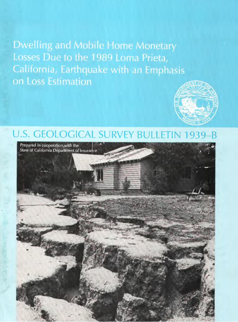
COVER: "***the cracks look like the stuff of nightmares. They snake through yards and across roadways .... [and] Summit Road from Highway 17 to Loma Prieta. The most impressive, three feet wide and seven feet deep, runs in front of John and Freda Tranbarger's house on Summit***". Photograph by Jim Gensheimer, October 24, 1989. Published November 30, 1989, in San Jose Mercury News and reproduced by permission. The photo, taken 7 days after the earthquake, shows water in the cracks due to the previous day's rainfall, thereby degrading the cracks.

Chapter B

Dwelling and Mobile Home Monetary Losses Due to the 1989 Loma Prieta, California, Earthquake with an Emphasis on Loss Estimation

By KARL V. STEINBRUGGE and RICHARD J. ROTH, JR.

Prepared in cooperation with theState of California Department of Insurance

U.S. GEOLOGICAL SURVEY BULLETIN 1939

ESTIMATION OF EARTHQUAKE LOSSES TO HOUSING IN CALIFORNIA

U.S. DEPARTMENT OF THE INTERIOR

BRUCE BABBITT, Secretary

U.S. GEOLOGICAL SURVEY

Gordon P. Eaton, Director

Any use of trade, product, or firm namesin this publication is for descriptive purposes onlyand does not imply endorsement by the U.S. Government

UNITED STATES GOVERNMENT PRINTING OFFICE, WASHINGTON : 1994

For sale byU.S. Geological Survey, Map Distribution Box 25286, MS 306, Federal Center Denver, CO 80225

Library of Congress Cataloging in Publication Data

Steinbrugge, Karl V.Dwelling and mobile home monetary losses due to the 1989 Loma Prieta

earthquake : with an emphasis on loss estimation / by Karl V. Steinbrugge and Richard J. Roth, Jr.

c. cm. (U.S. Geological Survey bulletin ; 1939-B) (Estimation of earthquake losses to housing in California ; ch. B)

"Prepared in cooperation with the State of California Department of Insurance."

Includes bibliographical references.1. Insurance, Earthquake California San Francisco Bay Region

Adjustment of claims. 2. Dwellings Earthquake effects California San Francisco Bay Region Costs. 3. Mobile homes Earthquake effects California San Francisco Bay Region Costs. 4. Earthquakes California Loma Prieta. 5. Earthquakes California San Francisco Bay Region. I. Roth, Richard J. II. California, Dept. of Insurance. III. Title. IV. Series. V. Series: Estimation of earthquake losses to housing in California ; ch. B. QE75.B9 no. 1939-B [HG9981.35.C2 557.3 s dc20[363.3'4] 94-33201

CIP

CONTENTS

Abstract Bl Acknowledgments Bl Wood frame dwellings B2

Introduction B2Characteristics of the earthquake B2 Seismic model B3 Terminology and definitions B3 Determining monetary losses from insurance data B5

Source A: California Department of Insurance B5 Source B B6Postal ZIP codes and distances from earthquakes B8

Dwelling losses before and after deductible B8 Probable maximum loss (PML) BIO

Definition of probable maximum loss (PML) BIO Definition of PML zone B12

Losses in the Loma Prieta PML zone B12 Losses by age groups B12 Elimination of losses due to major geohazards B13 PML and loss over deductible B14

Loss over deductible ZIP basis B15 Loss over deductible zone basis B18 Loss over deductible Watsonville study area basis B18 Loss over deductible other California experience B21 PMLs and equations for loss over deductible B22

Size of the PML zone B24Loma Prieta earthquake B24 Smaller magnitude earthquakes B24 1906 San Francisco earthquake B24

Estimation of loss over deductible and PMLs for other magnitudes B25 Post-1939 construction B25

1992 Landers earthquake: California residential earthquake recovery plandeductible B27

Pre-1940 construction B28 Dwelling contents losses B29 Additional living expense (Ale) for dwellings B31 Geographic distribution of losses B31 Construction and value as variables B33 Modified Mercalli intensity B35

Mobile homes (manufactured housing) B35 Introduction B35Definition of mobile home (manufactured housing) B35 Characteristic damage B37 Loma Prieta earthquake B37

Source B data B37 Source C data B41California Department of Housing and Community Development B43

Experience from previous earthquakes B45 1971 San Fernando earthquake B45

Observations on San Fernando B48 1978 Santa Barbara earthquake B49

Observations on Santa Barbara B51

Contents III

Mobile homes (manufactured housing) Continued Experience from previous earthquakes Continued

1979 El Centre (Imperial Valley) earthquake B51 Test of rapid loss estimation, El Centre B52

1980 Livermore (Greenville) earthquakes B521983 Coalinga earthquake B53

Synthesis and overview B54PML zone B54Loss over deductible in the PML zone B54Maximum losses in the PML zone B55Loss attenuation with distance B56Earthquake bracing B57Coach size and damage B57Loss estimation from rapid field inspections B57

Summary, major findings, and conclusions B57 Wood frame dwellings B57

Dwelling loss versus other losses B57PML zone and modified Mercalli intensities B57Dwelling age and loss B57Geohazards B58Deductibles B58Loss attenuation with distance B58Contents losses B58Ensuing fire B58Research needs B59

Mobile homes (manufactured housing) B59Nonbraced mobile homes B59Earthquake bracing B59Loss attenuation B59Research needs B59Comparative losses: Wood frame and mobile homes B59

References B59Appendix A. Sensitivity: Loss over deductible versus dwelling PML changes B61 Appendix B. Definitions of degree of damage to mobile homes B61

FIGURES

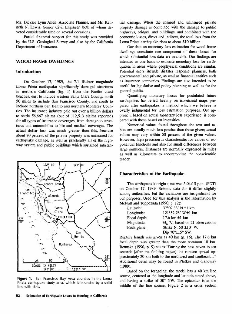
1. San Francisco Bay Area counties in the Loma Prieta earthquake study area, which is bounded by a solid line with dots. B2

2. Diagrammatic cross section through the fault (view is northwest) modeling the earthquake's line source and zone source of seismic energy. B3

3. Epicentral area of the Loma Prieta earthquake. The heavy black line is the surface projection of the modeled line source of the seismic energy. The diamond at the midpoint of the heavy black line is the epicenter. See figure 2 for the model of the line source. The closed loop about the heavy black line is the limit of the probable maximum loss zone (PML zone, defined in section "Definition of PML Zone"). B5

4. Postal ZIPs in epicentral area of the Loma Prieta earthquake. See figure 3 for relationships to the topography. ZIPs limited to portions of Santa Cruz and Santa Clara Counties. ZIP boundaries in the Santa Cruz Mountains are uncertain. Map adapted from "ZIP Codes in the San Francisco Bay Area" by permission of the copyright owner, Western Economic Research Co., Panorama City, California. Heavy black line and loop are explained in figure 3. B9

5. Percent loss over deductible at 10 percent deductible plotted against distance from the fault. See text for discussion. Watsonville study area is defined in section "Loss Over Deductible Watsonville Study Area" and in figure 7. B16

IV Contents

6. Average paid building loss per earthquake insured building plotted against distance from fault. See text for discussion. B18

7. Watsonville study area and Watsonville city limits. Solid triangles are locations of mobile home parks; park numbers are identified in table 26. Open circles are structures outside of the central business district posted as hazardous after the earthquake. B20

8. Loma Prieta and Coalinga loss over deductible data with each normalized at 10 percent deductible. Also shown is the range of normalized loss over deductible data for all ZIPs in the PML zone at 20 percent deductible. B22

9. Expansion of a portion of figure 8 including the Watsonville study area. The Wat­ sonville study area data essentially overlaid the Coalinga curve in figure 8. The solid circles are for the Loma Prieta PML zone. The open circles are for the Watsonville study area. B23

10. Loss over deductible for magnitudes 5 (threshold of building damage); magnitude 6.9 (equation 5, basis for equation 7); 7.75 (reasonable upper limit), and 8.25 (1906 San Francisco with no upper limit). Curves from equation 7 with uncertain­ ty factor of 1.0. B26

11. Equation 7 loss over deductible curve compared with Landers earthquake data. Upper right hand corner shows slope comparisons at 1 percent normalization. B28

12. Geographic distribution of average building loss as a percent of insured value using data source A information. Each open or solid circle represents the centroid of a postal ZIP having more than 10 wood frame earthquake insured buildings. Solid circles have, on an ZIP average basis, losses equalling or exceeding 0.5 percent. Open circles have lessor average losses or none. Solid circles with aver­ age losses equalling or exceeding 1.0 percent also show the percent loss. Data shown are from table 44 (at end of report) which differ slightly from those used in figure 5. B33

13. Another perspective on figure 12 data and those in table 44. The plot is paidbuilding loss plus deductible as a percent of value against distance from the fault. Loss percentages less than 0.5 percent are not plotted. B33

14. PML zone and its relationships to the Modified Mercalli intensity zone VIII. Also shown is the boundary of the ZIPs with centroids within the PML zone. B36

15. Loma Prieta earthquake. Mobile home loss over 10 percent deductible as a func­ tion of distance from the fault for parks are grouped by ZIP; in figure 16, parks are individually plotted. Excluded are ZIPs with no losses or fewer than 10 mo­ bile homes. Names are post office names and may include large rural areas. Data from source B. B38

16. Loma Prieta earthquake. Percent loss over 10 percent deductible as a function of distance from the fault for individual mobile home parks; in figure 15, parks are grouped by ZIP. Solid triangles are parks located in Watsonville ZIP 95076. Solid circles are parks in a coastal community, or nearby. Open circles are parks to the east of the fault, ranging from the Santa Clara Valley to Hollister. Data from source B. B39

17. Loma Prieta earthquake. Percent of fallen mobile homes as a function of distance from the fault. Numbers beside the solid circles are the park numbers identified in table 31. Source is California Department of Housing and Community Develop­ ment (1989?, p. 2). B45

18. 1971 San Fernando earthquake region showing the locations of mobile home parks. Numbers adjacent to the solid triangles are park numbers found in table 32. B47

19. 1971 San Fernando earthquake. Percent loss over deductible as a function of dis­ tance for individual mobile home parks. Numbers are park numbers identified in table 32. B48

20. 1978 Santa Barbara earthquake region showing epicenter and approximate location of the mobile home parks (solid circles). Numbers beside the circles are identified in table 35. B50

Contents

21. 1979 El Centre earthquake region showing mobile home parks (solid triangles). Numbers by the triangles are park numbers identified in table 36. B51

22. 1980 Livermore (Greenville) earthquake region showing approximate location of surface breakage associated with faulting. Numbers by the solid triangles are park numbers identified in the text. B52

23. Percent loss over deductible as a function of percent deductible. Curve for coaches is based on equation 11 for magnitude 7.75. That for coach and contents is based on equation 12, also for magnitude 7.75. B56

TABLES

1. Summary of insurance losses paid for all lines of insurance B62. Homeowner (Ho.) dwellings and paid earthquake (Eq.) losses B73. Percent of homeowner earthquake insured dwellings having paid losses B74. Percentage of homeowners policies also with earthquake coverage B85. Santa Cruz County paid losses (portion of computer hard copy) Bll6. Number of insured dwellings from source B data grouped by decade B127. Homeowner insured dwellings from source B data, with or without earthquake

coverage B138. Paid losses to dwellings with earthquake coverage grouped by decade B139. Geohazard grades for dwellings in source B data B14

10. Paid losses and values as function of percent deductible for dwellings in PML zone B15

11. Percent loss over deductible for dwellings in ZIPs 10 miles or less from the fault as a function of percent deductible (defined in table 10) B17

12. Effect of geohazards on loss over deductible in PML zone ZIPs B1913. Percentage loss over deductible data for 1989 Loma Prieta and 1983 Coalinga

earthquakes as a function of percent deductible B1914. Loss over deductible comparisons at 10 percent deductible B2115. Percentage loss over deductible as a function of percent deductible for varying

earthquake magnitudes B2716. Contents loss as percent of building loss as a function of percent deductible B2917. Contents loss as a percent of building value for nine-county study area B3018. Ale loss as percent of building loss as a function of percent deductible B3019. Building losses for selected ZIPs at distant locations B3120. Number of stories as a function of building losses B3421. Type of roof as a function of building losses B3422. Masonry chimneys as a function of building losses B3423. Value as a function of earthquake insurance coverage B3424. Mobile home (manufactured housing) losses in 14 counties B3725. Mobile home losses 10 miles or less from the fault B3826. Coach loss data on selected mobile home parks B4027. Type of foundation anchorage for mobile homes B4028. Relationships among losses and values for mobile home coaches, contents, and

Ale B4129. Mobile homes with paid losses in the PML zone B4230. Relationships among losses and values for mobile home coaches, contents, and

Ale B4231. Mobile home performance in the 1989 Loma Prieta earthquake, insurance and

non-insurance data B4432. Mobile home loss experience from 1971 San Fernando earthquake, magnitude

6.4 B4633. Average loss to mobile home components, 1971 San Fernando earthquake, magni­

tude 6.4 B49

VI Contents

34. Wood frame dwelling versus mobile home losses for 1971 San Fernando earth­ quake, magnitude 6.4, zero deductible B49

35. Average loss to mobile home components from 1978 Santa Barbara earthquake, magnitude 5.1 B50

36. Average loss to mobile home components from 1979 El Centro (Imperial Valley) earthquake, magnitude 6.4 B51

37. Mobile home damage from 1979 El Centro (Imperial Valley) earthquake, magni­ tude 6.4 B52

38. Mobile home damage in park 1 from 1980 Livermore (Greenville) earthquakes, magnitudes 5.5 and 5.6 B53

39. Mobile home damage from 1983 Coalinga earthquake, magnitude 6.7 B5340. Performance of mobile home supports in 1983 Coalinga earthquake, magnitude

6.7 B5341. Mobile home loss over deductible in PML zone B5442. Loss over deductible as a function of deductible, in percent B5543. Comparison of losses to mobile homes B5644. Building, contents, and Ale losses, before and after deductible B63

Contents VII

Dwelling and Mobile Home Monetary LossesDue to the 1989 Loma Prieta, California, Earthquake,with an Emphasis on Loss Estimation

By Karl V. Steinbrugge1 and Richard J. Roth, Jr. 2

Abstract

Our overall objective is to improve the methodology of monetary loss estimation for wood frame dwellings and mo­ bile homes by using earthquake insurance loss information based on specific data gathered after the Loma Prieta earth­ quake. Wherever applicable, it is intended to replace meth­ odologies based on the Modified Mercalli scale. Loss data used were gathered by the California Department of Insur­ ance and supplemented from other insurance sources. These data were compared and analyzed with similar information from all available California earthquakes.

Detailed loss data from the Loma Prieta earthquake were obtained from over 55,000 paid claims, which com­ prised all forms of insurance including those on dwellings. More detailed, supplementary information on 85,382 wood frame dwellings was obtained on loss (if any), construction variations, and many other components. Of these dwellings, 5,530 had paid losses in the study area, which includes nine counties in the San Francisco Bay area. Data are deliberately presented in considerable detail since they are difficult to obtain directly from our sources. Several are used by permis­ sion from proprietary sources or otherwise are not generally available. The strong and weak aspects of our data are pointed out.

Wood frame dwellings constructed prior to 1940 experi­ enced average losses exceeding twice those of later con­ struction. Post-1939 dwellings in the epicentral region suffered about 6 percent average building loss when not sub­ jected to landsliding or located on stable but steeply sloping sites. Average building losses at 10 miles from the fault were small, and at 20 miles were negligible. Major exceptions were in structurally poor ground areas with liquefiable soils,

Consulting Structural Engineer, El Cerrito, California. Chief Property/Casualty Actuary, California Department of Insur­

ance, Los Angeles, California.

Manuscript approved for publication July 20, 1994.

where losses were magnified. A prime example was San Francisco's Marina District, which was 50 miles away.

Deductibles are normal in insurance policies, whether private or government. They are also sometimes found in on£ form or another in governmental grants. We developed loss over deductible equations which relate average home- owner loss that is, the loss absorbed by the homeowner, beyond that covered by insurance. The equations are on an aggregate basis and not applicable to individual structures and are principally for computer use in broad loss estimation calculations.

When collapse did not occur, reported contents losses were about 20 to 25 percent of the reported building loss on the average, admitting wide variations in valuations and sus­ ceptibilities among building and contents.

Mobile homes (manufactured housing), when not earth­ quake braced, were prone to fall off their supports. Within 20 miles of the earthquake, about 15 percent of the approxi­ mately 2,500 fell from their supports. In sharp contrast, those braced to resist earthquake shaking had no known instances of falling.

ACKNOWLEDGMENTS

We appreciate the advice and guidance freely given by Dr. S.T. Algermissen, U.S. Geological Survey, espe­ cially on seismological aspects, including a review of the line source model representing the energy release from the Loma Prieta earthquake. His comments throughout the en­ tire development of the manuscript were valuable.

Special acknowledgment is due to Mr. Robert L. Ocfrnan, retired Assistant Vice President of the State Farm Fire and Casualty Company, for his thoughtful examina- tioh of the manuscript at various stages during its develop­ ment. His engineering background provided technical insights to the engineering aspects as well as to the nu­ ances of insurance company practices.

The City of Watsonville provided assistance and in­ sights during the examination of their original damage re­ ports and maps relating thereto. Special thanks are due to

Dwelling and Mobile Home Monetary Losses Due to the 1989 Loma Prieta, California, Earthquake, with an Emphasis on Loss Estimation B1

Ms. Dicksie Lynn Alien, Associate Planner, and Mr. Ken­ neth N. Lewis, Senior Civil Engineer, both of whom de­ voted considerable time on several occasions.

Partial financial support for this study was provided by the U.S. Geological Survey and also by the California Department of Insurance.

WOOD FRAME DWELLINGS

Introduction

On October 17, 1989, the 7.1 Richter magnitude Loma Prieta earthquake significantly damaged structures in northern California (fig. 1) from the Pacific coast beaches, east to include western Santa Clara County, north 50 miles to include San Francisco County, and south to include northern San Benito and northern Monterey Coun­ ties. The insurance industry paid out over a billion dollars to settle 56,667 claims (out of 112,513 claims reported) for all types of insurance coverages, from damage to struc­ tures and automobiles to life and medical coverages. The actual dollar loss was much greater than this, because about 70 percent of the private property was uninsured for earthquake damage, as well as practically all of the high­ way system and public buildings which sustained substan-

N 122.° 100' I j 121°] 00' .^'"' .x

\ f-* ' /' ^.J 7.^* /X

T^^' V / 3^:\ .' J£_! \ / 00>

^.^

SCALE, IN MILES _____122°100' \i2r'loo ;

Figure 1. San Francisco Bay Area counties in the Loma Prieta earthquake study area, which is bounded by a solid line with dots.

tial damage. When the insured and uninsured private property damage is combined with the damage to public highways, bridges, and buildings, and combined with the economic losses, direct and indirect, the total loss from the Loma Prieta earthquake rises to about $10 billion.

Our data on monetary loss estimation for wood frame dwellings constitute one component of these losses for which substantial loss data are available. Our findings are intended as one basis to estimate monetary loss for earth­ quakes in areas where geophysical conditions are similar. Potential users include disaster response planners, both governmental and private, as well as financial entities such as insurance companies. Findings are also intended to be useful for legislative and policy planning as well as for the general public.

Quantifying monetary losses for postulated future earthquakes has relied heavily on isoseismal maps pre­ pared after earthquakes, a method which we believe is overly judgmental for loss estimation purposes. Our ap­ proach, based on actual monetary loss experience, is com­ pared with those based on intensities.

Numerical values found throughout the text and ta­ bles are usually much less precise than those given; actual values may vary within 50 percent of the given values. However, high precision is characteristic for values of ex­ ponential functions and also for small differences between large numbers. Distances are normally expressed in miles as well as kilometers to accommodate the nonscientific reader.

Characteristics of the Earthquake

The earthquake's origin time was 5:04:15 p.m. (PDT) on October 17, 1989. Seismic data for it differ slightly among authorities, but the variations are insignificant for our purposes. Used for this analysis is the information by McNutt and Toppozada (1990, p. 12):

Latitude: 37°02.33' N.±l kmLongitude: 121°52.76' W.±l kmFocal depth: 17.6 km ±1 kmMagnitude: Ms 7.1 based on 21 observationsFault plane: Strike N. 50°±10° W.

Dip 70°±15° SW.Rupture length was given as 40 km (p. 16). The 17.6 km focal depth was greater than the more common 10 km. Benuska (1990, p. 9) states "During the next seven to ten seconds [after the faulting began] the rupture spread ap­ proximately 20 km both to the northwest and southeast...." Additional detail may be found in Plafker and Galloway (1989).

Based on the foregoing, the model has a 40 km line source, centered at the longitude and latitude stated above, and having a strike of 50° NW. The epicenter is at the middle of the line source. Figure 2 is a cross section

B2 Estimation of Earthquake Losses to Housing in California

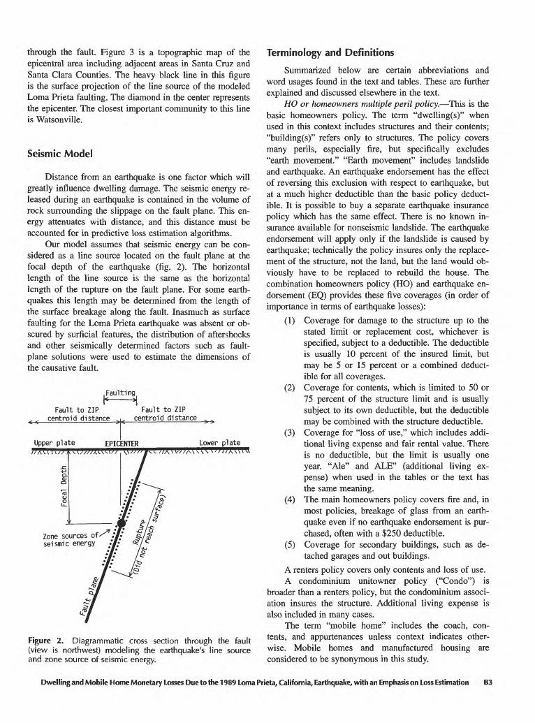
through the fault. Figure 3 is a topographic map of the epicentral area including adjacent areas in Santa Cruz and Santa Clara Counties. The heavy black line in this figure is the surface projection of the line source of the modeled Loma Prieta faulting. The diamond in the center represents the epicenter. The closest important community to this line is Watsonville.

Seismic Model

Distance from an earthquake is one factor which will greatly influence dwelling damage. The seismic energy re­ leased during an earthquake is contained in the volume of rock surrounding the slippage on the fault plane. This en­ ergy attenuates with distance, and this distance must be accounted for in predictive loss estimation algorithms.

Our model assumes that seismic energy can be con­ sidered as a line source located on the fault plane at the focal depth of the earthquake (fig. 2). The horizontal length of the line source is the same as the horizontal length of the rupture on the fault plane. For some earth­ quakes this length may be determined from the length of the surface breakage along the fault. Inasmuch as surface faulting for the Loma Prieta earthquake was absent or ob­ scured by surficial features, the distribution of aftershocks and other seismically determined factors such as fault- plane solutions were used to estimate the dimensions of the causative fault.

.Faulting

Fault to ZIP Fault to ZIP centroid distance ^ centrold distance ^

Upper plate EPICENTER Lower plate

Zone sources seismic energy

Figure 2. Diagrammatic cross section through the fault (view is northwest) modeling the earthquake's line source and zone source of seismic energy.

Terminology and Definitions

Summarized below are certain abbreviations and word usages found in the text and tables. These are further explained and discussed elsewhere in the text.

HO or homeowners multiple peril policy. This is the basic homeowners policy. The term "dwelling(s)" when used in this context includes structures and their contents; "building(s)" refers only to structures. The policy covers many perils, especially fire, but specifically excludes "earth movement." "Earth movement" includes landslide and earthquake. An earthquake endorsement has the effect of reversing this exclusion with respect to earthquake, but at a much higher deductible than the basic policy deduct­ ible. It is possible to buy a separate earthquake insurance policy which has the same effect. There is no known in­ surance available for nonseismic landslide. The earthquake endorsement will apply only if the landslide is caused by earthquake; technically the policy insures only the replace­ ment of the structure, not the land, but the land would ob­ viously have to be replaced to rebuild the house. The combination homeowners policy (HO) and earthquake en­ dorsement (EQ) provides these five coverages (in order of importance in terms of earthquake losses):

(1) Coverage for damage to the structure up to the stated limit or replacement cost, whichever is specified, subject to a deductible. The deductible is usually 10 percent of the insured limit, but may be 5 or 15 percent or a combined deduct­ ible for all coverages.

(2) Coverage for contents, which is limited to 50 or 75 percent of the structure limit and is usually subject to its own deductible, but the deductible may be combined with the structure deductible.

(3) Coverage for "loss of use," which includes addi­ tional living expense and fair rental value. There is no deductible, but the limit is usually one year. "Ale" and ALE" (additional living ex­ pense) when used in the tables or the text has the same meaning.

(4) The main homeowners policy covers fire and, in most policies, breakage of glass from an earth­ quake even if no earthquake endorsement is pur­ chased, often with a $250 deductible.

(5) Coverage for secondary buildings, such as de­ tached garages and out buildings.

A renters policy covers only contents and loss of use.A condominium unitowner policy ("Condo") is

broader than a renters policy, but the condominium associ­ ation insures the structure. Additional living expense is also included in many cases.

The term "mobile home" includes the coach, con­ tents, and appurtenances unless context indicates other­ wise. Mobile homes and manufactured housing are considered to be synonymous in this study.

Dwelling and Mobile Home Monetary Losses Due to the 1989 Loma Prieta, California, Earthquake, with an Emphasis on Loss Estimation B3

Determining Monetary Losses from Insurance Data

Paid insurance claims provide a substantially im­ proved basis for monetary loss estimation of future earth­ quakes for two reasons. First, paid insurance claims represent the cost of repair and are therefore a direct measure of vulnerability. In contrast, when vulnerability is derived from physical damage, estimates of cost of repair must be made (of the various damaged structural and non- structural components of a building, including depreciation if applicable) to calculate costs. Consequently, it is much more difficult to determine the percentage loss or cost of repair from damage data than it is from paid insurance claims. Second, cost of repair data need not be referenced to Modified Mercalli intensity for use in determining vul­ nerability. The use of paid insurance claims as the basis for building vulnerability relationships was suggested by Steinbrugge and others (1984).

Normally, private insurance has a deductible clause, wherein the insurer shares losses with the owner. This is also generally true in some related form where governmental insurance or assistance program is provided. Aggregate loss estimates for future earthquakes must necessarily consider the impact of deductibles (Steinbrugge, 1990). A percentage deductible is used in this study; percentages may readily be changed to dollars or to various combinations of dollars and percentages through simple mathematical computations.

Despite the advantages of using paid earthquake in­ surance claims, they have some disadvantages. The data base of paid claims that have been analyzed is restricted to California. Also, the location of each large claim should be field checked to ascertain if the claim is a result of only ground shaking or if ground failure such as landsliding or liquefaction has been a factor.

The Loma Prieta earthquake provided an unusual op­ portunity to examine relationships among values, monetary losses, and monetary loss attenuation with distance for dwellings and mobile homes. This event is unique in United States experience in that it has been the largest magnitude earthquake to date for which substantial amounts of reliable quantitative monetary loss data are available. [Note added in press: When monetary losses become available for the 1994 Northridge, California, earthquake, they are expected to exceed those of Loma Prieta.]

The Loma Prieta study area is confined to nine coun­ ties (fig. 1) around the San Francisco Bay and Monterey Bay, as follows:

^ Figure 3. Epicentral area of the Loma Prieta earth­ quake. The heavy black line is the surface projection of the modeled line source of the seismic energy. The diamond at the midpoint of the heavy black line is the epicenter. See figure 2 for the model of the line source. The closed loop about the heavy black line is the limit of the probable maxi­ mum loss zone (PML zone, defined in section "Definition of PML Zone").

Alameda Contra Costa Marin

Monterey San Benito San Francisco

San Mateo Santa Clara Santa Cruz

Reliable insurance loss information came from two principal sources which are described below.

Source A: California Department of Insurance

On January 31, 1990, the California Department of Insurance issued a special data call for loss statistics relat­ ing to the Loma Prieta earthquake to all insurers licensed to do business in the State of California. Under the depart­ ment's general regulatory authority, all insurers were re­ quired to respond. On February 15, 1991, the department issued a second data call to update the information from the first data call. This time, the insurers reported that the total incurred losses for all coverages as $901,762,236 on a total of 56,667 claims. No further information was requested from the insurers. No insurer became insolvent because of this earthquake. Information from this latter data call is referred to as "Source A" throughout this study.

Table 1 is a summary of some of the results received from 212 insurer groups. Most groups in turn have several licensed insurers, but under common management, and so the total number of insurers reporting actual losses was much greater. There are about 1,500 insurers licensed in California, half life and health and half property/casualty. The remaining insurers had few or no losses. The five larg­ est groups paid out 70 percent of the residential losses, and the 15 largest groups paid out 90 percent of the residential losses. The fire losses are separately stated in table 1, since they are not covered under an earthquake policy but are paid under many lines of insurance in addition to the "fire" line of insurance. For instance, a loss under an earthquake endorsement attached to a homeowners policy may be allo­ cated to the homeowner's line or to the earthquake line with any ensuing fire loss allocated to the homeowners line. Also, it is possible to have losses under a homeowners policy whether or not there was an earthquake endorsement (for example, for glass breakage or fire).

It is important to reiterate that our loss estimation study of wood frame dwellings is based on insurance data. For the Loma Prieta study area, our data base is limited because only 30 to 35 percent of the dwellings had earthquake insurance; many owners of low-value dwellings, brick homes, or older homes perhaps chose not to insure because of the cost. Nevertheless, it does not appear that our results are seriously impacted by this shortcoming. In particular, the geographic distribution of insured dwellings seems to be fairly even. Another limitation to our data was that the amount the in­ surer paid was subject to the provisions of the insurance

Dwelling and Mobile Home Monetary Losses Due to the 1989 Loma Prieta, California, Earthquake, with an Emphasis on Loss Estimation B5

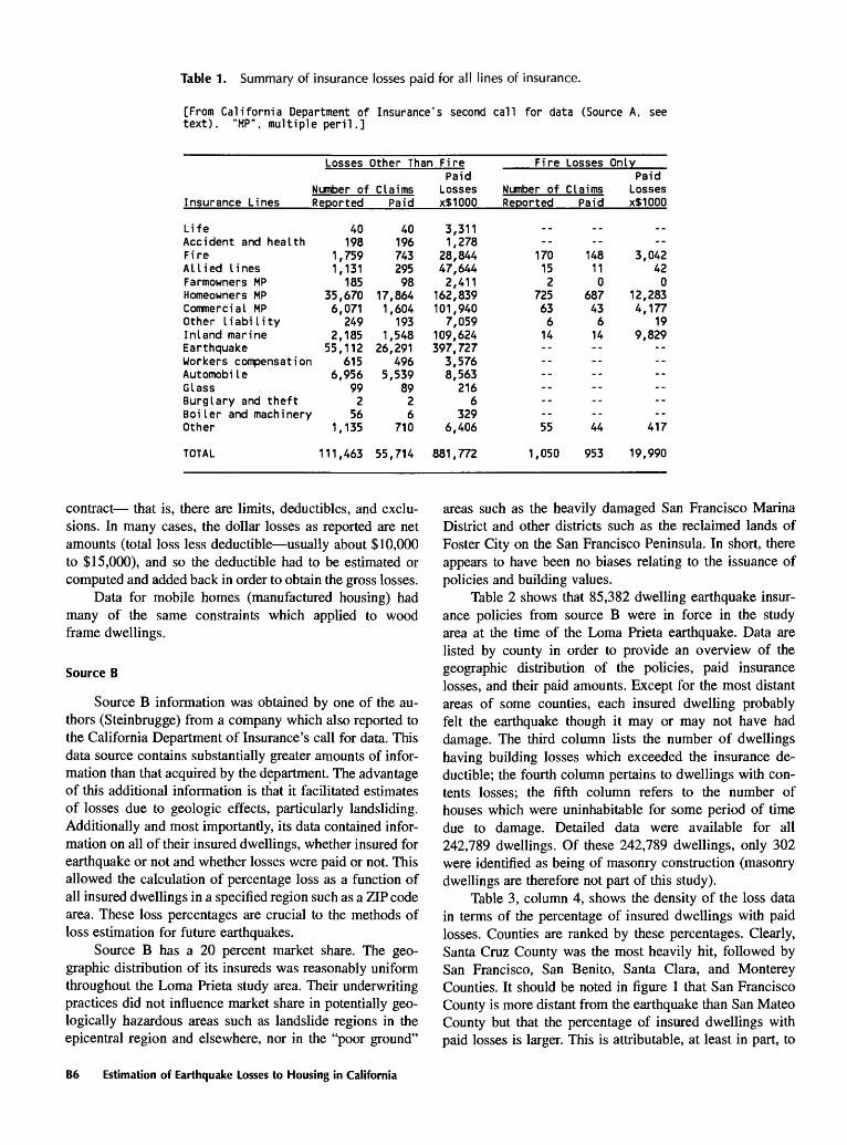
Table 1. Summary of insurance losses paid for all lines of insurance.

[From California Department of Insurance's second call for data (Source A, see text). "MP". multiple peril.]

Insurance Lines

LifeAccident and healthFireAllied linesFarmowners MPHomeowners MPCommercial MPOther liabilityInland marineEarthquakeWorkers compensationAutomobi leGlassBurglary and theftBoiler and machineryOther

Losses

Number of Reported

40198

1,7591,131

18535,6706,071

2492,185

55,112615

6,956992

561,135

Other Than Fire

Claims Paid

4019674329598

17,8641,604

1931,548

26,291496

5,5398926

710

Paid Losses x$1000

3,3111,278

28,84447,6442,411

162,839101,9407,059

109,624397,727

3,5768,563

2166

3296,406

Fire

Number ofReported

..--

170152

725636

14------------55

Losses Only

ClaimsPaid

--148110

687436

14------------44

Paid Losses x$1000

..--

3,042420

12,2834,177

199,829

------------

417

TOTAL 111,463 55,714 881,772 1,050 953 19,990

contract that is, there are limits, deductibles, and exclu­ sions. In many cases, the dollar losses as reported are net amounts (total loss less deductible usually about $10,000 to $15,000), and so the deductible had to be estimated or computed and added back in order to obtain the gross losses.

Data for mobile homes (manufactured housing) had many of the same constraints which applied to wood frame dwellings.

Source B

Source B information was obtained by one of the au­ thors (Steinbrugge) from a company which also reported to the California Department of Insurance's call for data. This data source contains substantially greater amounts of infor­ mation than that acquired by the department. The advantage of this additional information is that it facilitated estimates of losses due to geologic effects, particularly landsliding. Additionally and most importantly, its data contained infor­ mation on all of their insured dwellings, whether insured for earthquake or not and whether losses were paid or not. This allowed the calculation of percentage loss as a function of all insured dwellings in a specified region such as a ZIP code area. These loss percentages are crucial to the methods of loss estimation for future earthquakes.

Source B has a 20 percent market share. The geo­ graphic distribution of its insureds was reasonably uniform throughout the Loma Prieta study area. Their underwriting practices did not influence market share in potentially geo­ logically hazardous areas such as landslide regions in the epicentral region and elsewhere, nor in the "poor ground"

areas such as the heavily damaged San Francisco Marina District and other districts such as the reclaimed lands of Foster City on the San Francisco Peninsula. In short, there appears to have been no biases relating to the issuance of policies and building values.

Table 2 shows that 85,382 dwelling earthquake insur­ ance policies from source B were in force in the study area at the time of the Loma Prieta earthquake. Data are listed by county in order to provide an overview of the geographic distribution of the policies, paid insurance losses, and their paid amounts. Except for the most distant areas of some counties, each insured dwelling probably felt the earthquake though it may or may not have had damage. The third column lists the number of dwellings having building losses which exceeded the insurance de­ ductible; the fourth column pertains to dwellings with con­ tents losses; the fifth column refers to the number of houses which were uninhabitable for some period of time due to damage. Detailed data were available for all 242,789 dwellings. Of these 242,789 dwellings, only 302 were identified as being of masonry construction (masonry dwellings are therefore not part of this study).

Table 3, column 4, shows the density of the loss data in terms of the percentage of insured dwellings with paid losses. Counties are ranked by these percentages. Clearly, Santa Cruz County was the most heavily hit, followed by San Francisco, San Benito, Santa Clara, and Monterey Counties. It should be noted in figure 1 that San Francisco County is more distant from the earthquake than San Mateo County but that the percentage of insured dwellings with paid losses is larger. This is attributable, at least in part, to

B6 Estimation of Earthquake Losses to Housing in California

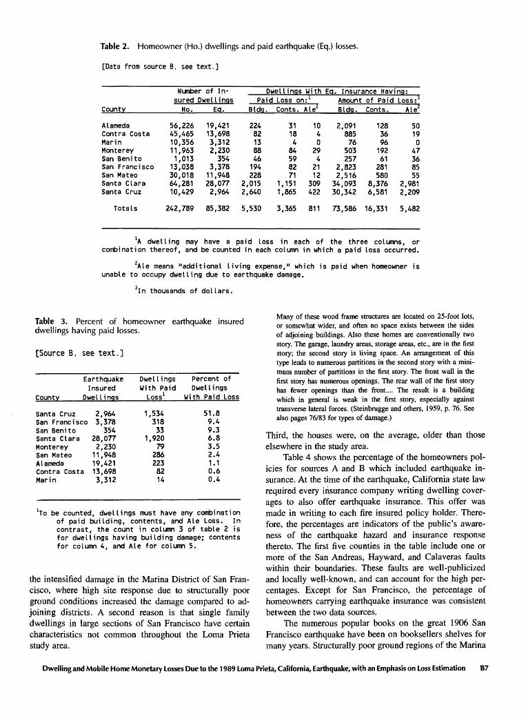
Table 2. Homeowner (Ho.) dwellings and paid earthquake (Eq.) losses.

[Data from source B, see text.]

County

AlamedaContra CostaMar inMontereySan BenitoSan FranciscoSan MateoSanta ClaraSanta Cruz

Number of In- sured Dwel lings

Ho. Ed.

56,22645,46510,35611,9631,013

13,03830,01864,28110,429

19,42113,6983,3122,230354

3,37811,94828,0772,964

Dwellings With Eq. Insurance Having:Paid Loss on: 1

Bldq.

22482138846194228

2,0152,640

Conts.

31184

84598271

1,1511,865

Ale2

1040

294

2112

309422

AmountBldq.

2,09188576

503257

2,8232,516

34,09330,342

of PaidConts.

128369619261

281580

8,3766,581

Loss: 3Ale4

50190

47368555

2,9812,209

Totals 242,789 85,382 5,530 3,365 811 73,586 16,331 5,482

:A dwelling may have a paid loss in each of the three columns, or combination thereof, and be counted in each column in which a paid loss occurred.

2Ale means "additional living expense," which is paid when homeowner is unable to occupy dwelling due to earthquake damage.

3 In thousands of dollars.

Table 3. Percent of homeowner earthquake insured dwellings having paid losses.

[Source B, see text.]

Earthquake Insured

County Dwellings

Santa CruzSan FranciscoSan BenitoSanta ClaraMontereySan MateoAlamedaContra CostaMar in

2,9643,378

35428,0772,23011,94819,42113,6983,312

Dwellings With Paid Loss 1

1,53431833

1,92079

2862238214

Percent of Dwellings

With Paid Loss

51.89.49.36.83.52.41.10.60.4

be counted, dwellings must have any combination of paid building, contents, and Ale Loss. In contrast, the count in column 3 of table 2 is for dwellings having building damage; contents for column 4, and Ale for column 5.

the intensified damage in the Marina District of San Fran­ cisco, where high site response due to structurally poor ground conditions increased the damage compared to ad­ joining districts. A second reason is that single family dwellings in large sections of San Francisco have certain characteristics not common throughout the Loma Prieta study area.

Many of these wood frame structures are located on 25-foot lots, or somewhat wider, and often no space exists between the sides of adjoining buildings. Also these homes are conventionally two story. The garage, laundry areas, storage areas, etc., are in the first story; the second story is living space. An arrangement of this type leads to numerous partitions in the second story with a mini­ mum number of partitions in the first story. The front wall in the first story has numerous openings. The rear wall of the first story has fewer openings than the front.... The result is a building which in general is weak in the first story, especially against transverse lateral forces. (Steinbrugge and others, 1959, p. 76. See also pages 76/83 for types of damage.)

Third, the houses were, on the average, older than those elsewhere in the study area.

Table 4 shows the percentage of the homeowners pol­ icies for sources A and B which included earthquake in­ surance. At the time of the earthquake, California state law required every insurance company writing dwelling cover­ ages to also offer earthquake insurance. This offer was made in writing to each fire insured policy holder. There­ fore, the percentages are indicators of the public's aware­ ness of the earthquake hazard and insurance response thereto. The first five counties in the table include one or more of the San Andreas, Hayward, and Calaveras faults within their boundaries. These faults are well-publicized and locally well-known, and can account for the high per­ centages. Except for San Francisco, the percentage of homeowners carrying earthquake insurance was consistent between the two data sources.

The numerous popular books on the great 1906 San Francisco earthquake have been on booksellers shelves for many years. Structurally poor ground regions of the Marina

Dwelling and Mobile Home Monetary Losses Due to the 1989 Loma Prieta, California, Earthquake, with an Emphasis on Loss Estimation B7

Table 4. Percentage of homeowners policies also with earthquake coverage.

[Sources A and B. see text.]

Source B

County

Number of Percent of Homeowner Homeowners Policies With EQ. Coverage

Source ANumber of Percent ofHomeowner HomeownersPolicies With Eg. Coverage

Santa ClaraSan MateoSan BenitoA I amedaContra CostaMar inSanta CruzSonoma 1San FranciscoMontereySolano1Napa1San Joaquin1Sacramento1

81,31437,9441,210

70,21055,14913,82212,50220,03021,11814,87317,4576,05716,38040,401

34.531.529.327.724.824.023.720.716.015.013.79.35.24.1

252,721120,3633,657

203,365160,42542,03037,593

...79,382

...40,66017,804

...

31.631.827.427.821.324.022.5...

26.5---

14.110.7...

Bounties contiguous to the study area.

and Mission districts of San Francisco are on maps avail­ able to the public. As mentioned above, the prevailing type of wood frame construction in San Francisco is more vul­ nerable to earthquake damage than elsewhere in the Loma Prieta study area.

The last two counties in table 4 are located in Califor­ nia's Central Valley and have a lower seismicity than the other counties. The percentages for these two counties rea­ sonably reflect the public's perception of this lower hazard.

Additional data from several other companies have been used to fill voids or to otherwise strengthen the loss estimation analyses. These instances are mentioned where they occur.

Postal Zip Codes and Distances from Earthquakes

One direction of this study is to develop loss estima­ tion algorithms which are transferable to other regions under practical conditions. For loss estimation purposes and also for disaster response planning, dwelling data are nor­ mally more available on a postal ZIP basis than on other geographic bases. Some sources, such as the national cen­ sus, can be readily converted to a ZIP basis. ZIP boundaries may extend beyond city boundaries; as a consequence, the area included in a ZIP by its postal name may also include nearby small communities. ZIPs usually contain a sufficient number of dwelling losses to be statistically significant with the distance attenuated loss percentages.

For the Loma Prieta study area, distances were com­ puted to each ZIP's geographic centroid. Locations of geo­ graphic centroids are essentially identical to those of housing centroids for the usual ZIP, but errors may occur

when large uninhabited areas are included. The term "ZIP to fault" distance or "fault distance" is defined as the short­ est distance from the surface projection of the earthquake's line source to the ZIP's population weighted centroid. An exception to this definition is for mobile home parks, where in some instances the distance from the line source is that from the park rather than from its ZIP centroid.

Figure 4 is a map of ZIPs in the vicinity of the Loma Prieta earthquake. The heavy black straight line with the diamond in the center has the same meaning as that in figure 3. The closed loop about the heavy black line is the 6 mile probable maximum loss (PML) zone; this will be further defined and discussed. ZIP boundaries within the Santa Cruz Mountains seem to have been in a state of flux at the time of the earthquake, inasmuch as four published ZIP maps and atlases were examined and each had differ­ ent boundaries for ZIP 95030 within the Santa Cruz Mountains. Other ZIP boundaries in the mountains also had uncertainties, but to a smaller degree. The boundary uncertainties do not affect our distance calculations since the centroids were determined on a population weighted basis. Additionally the uncertain boundaries are in very lightly populated areas. Also, for reasons discussed later, ZIP 95030 was eliminated from the loss over deductible analysis and resulting equations.

Dwelling Losses Before and after Deductible

As has been mentioned before, the detail of the infor­ mation on individual dwellings found in source B exceeds that in source A. Table 5 shows paid loss data from source

B8 Estimation of Earthquake Losses to Housing in California

15' SJ-

94304

:" *' "\ .f!/*'.f&V'. *' '" ' '*" . .-*' 95131 \I \ /.'.y'-K/' 94086 t 95054 ;.. .. /...-\

94024 ' » \ >: ^ \ '":. .. '*94087 *' Q50RO ?.. ^V « ' ,«&

95051

95014 I 95129 .;.;

951304-": 95008 "''\

95128'/. .: \.\ \.

: ''--".' 95125 .^ \

95136

95070/ *'* .-./ 95124 \ ^ : " "

' : V* ^ 95123

9503295120

122°|00'

ZIP POST OFFICE ZIP POST OFFICE

9402094024940409404194086940879430495003950059500695007950089501095014950179501895019950209502695030950329503795041950449504695050

La Honda Los Altos Mountain View Mountain View Sunnyvale Sunnyvale Palo Alto Aptos Ben Lomond Boulder Creek Brookdale Campbell Capitol a Cupertino Davenport Pel ton Freedom Gilroy Holy City Los Gatos Los Gatos Morgan Hill Mt. Hermon Redwood Estates San Martin Santa Clara

9505195054950609506295064950659506695070950739507695110951129511695117951189512095123951249512595126951289512995130951319513395136

Santa ClaraSanta ClaraSanta CruzSanta CruzUniv. CaliforniaSanta CruzScotts ValleySaratogaSoquelwatsonvilleSan JoseSan JoseSan JoseSan JoseSan JoseSan Jose ,37;San Jose 15'San JoseSan JoseSan JoseSan JoseSan JoseSan JoseSan JoseSan JoseSan Jose

121°145'

95030 J95037

.%.. .... ' ,9504l/ ";

95066 ''

SanBenito County

121°145'

Figure 4. Postal ZIPs in epicentral area of ZIPs limited to portions of Santa Cruz and tain. Map adapted from "ZIP Codes in th Economic Research Co., Panorama City,

the Loma Prieta earthquake. See figure 3 for relationships to the topography. Santa Clara Counties. ZIP boundaries in the Santa Cruz Mountains are uncer- 3 San Francisco Bay Area" by permission of the copyright owner, Western

California. Heavy black line and loop are explained in figure 3.

B for 45 dwellings of the 2,888 insured dwellings in Santa Cruz County. Losses include those paid under earthquake and/or homeowners policies, under condominium policies,

and under HO tenants (renters) policies. Specifically shown is a portion of ZIP 95003, which extends north from Monterey Bay into the Santa Cruz Mountains. Aptos

Dwelling and Mobile Home Monetary Losses Du<; to the 1989 Loma Prieta, California, Earthquake, with an Emphasis on Loss Estimation B9

and Rio Del Mar are in this ZIP, as are mountainous rural areas. Table 5 dwellings are in Santa Cruz County, where the highest percentage of paid losses was found (table 3).

Column 1 is the dwelling's ZIP. Column 2 is year built. Columns 3 and 4 are the dollar deductibles (HO for homeowners; EQ for earthquake). The "9" in column 5 indicates that the number of brick masonry chimneys is unknown; other numbers indicate number of chimneys. Column 6 gives the number of stories H means one and a half, and U or blank means unknown; coding available includes B for bi-level, I for two and a half, and T for tri- level (none of these shown on this page of table 5). In column 7, K is wood shake, W is wood shingle, U is un­ known, T is clay tile, and C is concrete tile; blank means unknown. Columns 8 and 9 are the amounts ("LIMIT") of fire insurance coverage. "EQ Blanket" in column 10 is the amount of earthquake insurance coverage; fire insurance coverage represents dwelling value, whereas earthquake coverage may be written for any amount at $100,000 or over for HO (non-tenant) and $10,000 or over for tenant and condo. Column 11 is the percentage of insurance to value; this allows revision of column 8 values when a homeowner insured a dwelling for something less than value. Contents limits do not allow this kind of revision. Column 18 (next to last column) is the occupancy desig­ nation: T for tenant (only contents insured); C for condo­ minium unit owner; and N for non-tenant (home owner).

Table 44 (at end of report) is a summary of loss data by ZIP in ZIP-fault distance order for the Loma Prieta study area. A negligible number of corrections and dele­ tions was made to the source data, mostly to dwellings which were incorrectly coded as to location. ZIPs with few insured dwellings are normally ZIPs assigned to post office boxes, to governmental entities, or to organizations with very high mail uses.

The meanings of table headings for table 5 also apply here, with these additions. "Cover" is an insurance term for insurance coverage, that is, an insurance policy. "CONTS." refers to the contents of the building.

Earthquake losses could be paid under either the earthquake policy ("EQ COVER") and/or under the home- owner policy ("HO COVER") owing to policy wording and differences in deductibles. ZIP 95030 had the heaviest losses because of geologic hazards in the Santa Cruz Mountains. Methods for computing the values in columns 7, 12, 28, 29, and 30 are shown at the bottom of the last page of table 44.

The insurance deductible used by source B differed considerably from that used by source A companies. Source B allowed the insured to purchase a different amount of earthquake insurance from that for fire. The amount of earth­ quake insurance for HO (non-tenant) could be between $100,000 (the minimum) and the amount of building and contents for fire insurance plus an amount for ALE (addi­ tional living expense). For tenants and condo unitowners, a

minimum of $10,000 applies to the earthquake coverage and additional limits may be purchased. The earthquake deduct­ ible was 10 percent of the amount of earthquake coverage and not of the fire coverage and is applied in dollars to the total earthquake loss. Claims practice allowed the determi­ nation of what portion of the deductible was applied to the building, contents, or ALE loss. For example, assume a person has a $200,000 dwelling with fire insurance and it was insured to full value. Were that person to chose $150,000 in earthquake insurance coverage, the earthquake deductible would be $15,000. This is 7.5 percent in terms of dwelling value. In a few instances, deductibles for Loma Prieta dwellings with paid losses became as low as 2 percent and 3 percent of building value.

It should be noted in passing that loss figures may be compiled somewhat differently by different companies, depending upon the adjustment practices. Should a dwell­ ing become a total loss, the order in which a deductible is applied to the building, to its contents, and to additional living expense may cause one or more of these three loss components to be underestimated. This discrepancy in methods can cause differences in loss values.

Probable Maximum Loss (PML)

It is intended to use Loma Prieta losses as a basis for estimating the probable maximum losses for a probable maximum earthquake. This process and its analysis is cov­ ered in following sections.

Definition of Probable Maximum Loss (PML)

"Probable maximum loss" (PML) is a term com­ monly used in California earthquake insurance loss esti­ mation. The California Department of Insurance (1981, p. 6) defined the geologic aspects of PML in "California Earthquake Zoning and Probable Maximum Loss Evalua­ tion Program," as follows:

The probable maximum loss for an individual building is that monetary loss expressed in dollars (or as a percentage of insured value) under the following conditions:

(a). Located on firm alluvial ground or on equivalent compacted man-made fills in a probable maximum loss zone [defined later], and

(b). Subjected only to the vibratory motion from the maximum probable earthquake, that is, not astride a fault or in a resulting landslide.

The California Department of Insurance has changed a portion of its original definition of PML to a loss over deductible approach. See Steinbrugge and Algermissen (1990) in the sections "Loss Over Deductible Approach" (p. A60) and "Applications to Simpler Methods" (p. A61) for the basis for the change.

Wood frame dwellings meeting these criteria in the probable maximum loss zone (PML zone) are grouped

B10 Estimation of Earthquake Losses to Housing in California

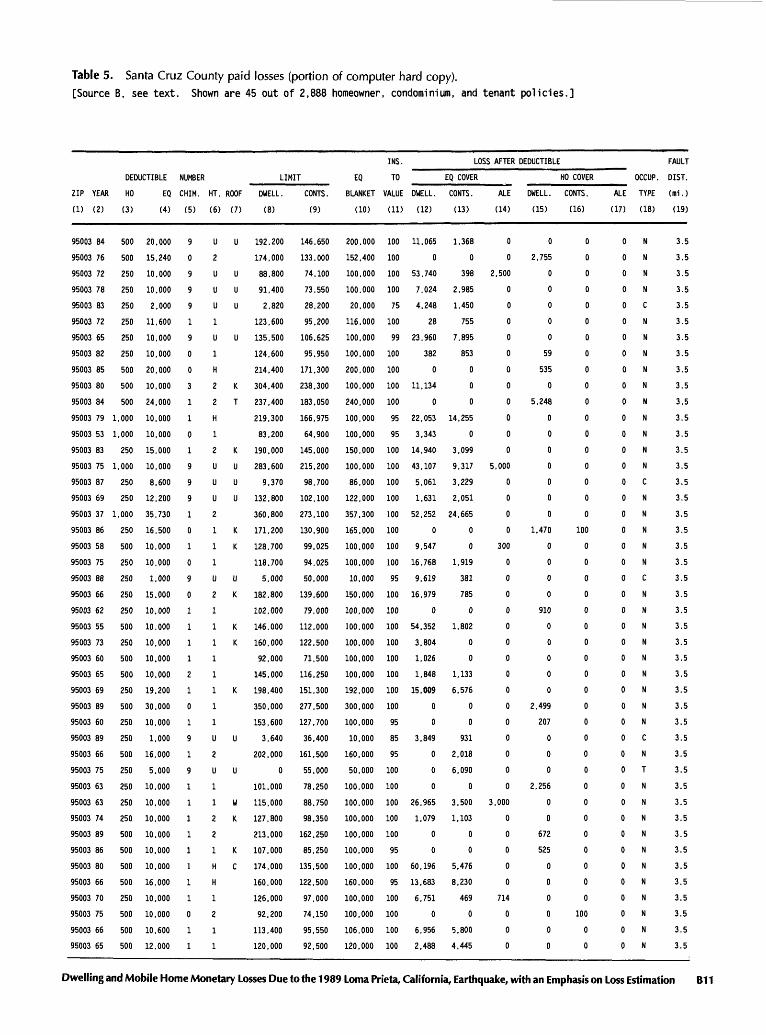
Table 5. Santa Cruz County paid losses (portion of computer hard copy),[Source B, see text. Shown are 45 out of 2,888 homeowner, condominium, and tenant policies.]

ZIP YEAR

(1) (2)

95003 84

95003 76

95003 72

95003 78

95003 83

95003 72

95003 65

95003 82

95003 85

95003 80

95003 84

95003 79

95003 53

95003 83

95003 75

95003 87

95003 69

95003 37

95003 86

95003 58

95003 75

95003 88

95003 66

95003 62

95003 55

95003 73

95003 60

95003 65

95003 69

95003 89

95003 60

95003 89

95003 66

95003 75

95003 63

95003 63

95003 74

95003 89

95003 86

95003 80

95003 66

95003 70

95003 75

95003 66

95003 65

DEDUCTIBLE

HO EQ

(3) (4)

500

500

250

250

250

250

250

250

500

500

500

1.000

1,000

250

1,000

250

250

1,000

250

500

250

250

250

250

500

250

500

500

250

500

250

250

500

250

250

250

250

500

500

500

500

250

500

500

500

20,000

15,240

10.000

10.000

2,000

11,600

10,000

10.000

20.000

10.000

24,000

10.000

10,000

15.000

10,000

8.600

12.200

35.730

16,500

10,000

10.000

1.000

15.000

10,000

10,000

10,000

10.000

10,000

19.200

30.000

10,000

1,000

16.000

5.000

10.000

10,000

10.000

10,000

10,000

10,000

16.000

10.000

10.000

10.600

12.000

NUMBER

CHIM. HT.

(5) (6)

9

0

9

9

9

1

9

0

0

3

1

1

0

1

9

9

9

1

0

1

0

9

0

1

1

1

1

2

1

0

1

9

1

9

1

1

1

1

1

1

1

1

0

1

1

u2

U

U

u1u1H

2

2

H

1

2

U

U

U

2

1

1

1

U

2

1

1

1

1

1

1

1

1

U

2

U

1

1

2

2

1

H

H

1

2

1

1

LIMIT

ROOF

(7)

U

U

U

U

U

K

T

K

U

U

U

K

K

U

K

K

K

K

U

U

W

K

K

C

DWELL.

(8)

192.200

174.000

88.800

91,400

2.820

123.600

135.500

124.600

214.400

304.400

237,400

219,300

83,200

190,000

283.600

9.370

132,800

360,800

171,200

128.700

118.700

5.000

182.800

102.000

146.000

160.000

92.000

145,000

198,400

350,000

153.600

3.640

202,000

0

101,000

115,000

127.800

213,000

107.000

174,000

160.000

126.000

92,200

113,400

120.000

CONTS.

(9)

146,650

133,000

74,100

73,550

28.200

95,200

106.625

95,950

171,300

238,300

183,050

166,975

64.900

145.000

215,200

98.700

102.100

273.100

130.900

99.025

94.025

50,000

139,600

79,000

112.000

122,500

71.500

116,250

151,300

277.500

127,700

36,400

161,500

55.000

78.250

88.750

98,350

162.250

85,250

135.500

122,500

97.000

74,150

95,550

92.500

EQ

BLANKET

(10)

200.000

152.400

100,000

100.000

20,000

116,000

100,000

100.000

200,000

100,000

240.000

100.000

100.000

150.000

100,000

86,000

122.000

357.300

165,000

100,000

100,000

10.000

150,000

100,000

100.000

100.000

100.000

100,000

192.000

300.000

100.000

10,000

160,000

50,000

100.000

100.000

100,000

100.000

100.000

100,000

160.000

100.000

100,000

106.000

120.000

INS.

TO

VALUE

(11)

100

100

100

100

75

100

99

100

100

100

100

95

95

100

100

100

100

100

100

100

100

95

100

100

100

100

100

100

100

100

95

85

95

100

100

100

100

100

95

100

95

100

100

100

100

LOSS AFTER

DWELL.

(12)

11,065

0

53,740

7.024

4,248

28

23.960

382

0

11.134

0

22,053

3.343

14,940

43,107

5.061

1.631

52.252

0

9.547

16.768

9.619

16,979

0

54.352

3,804

1,026

1,848

15.009

0

0

3,849

0

0

0

26,965

1.079

0

0

60.196

13,683

6,751

0

6.956

2,488

EQ COVER

CONTS.

(13)

1.368

0

398

2,985

1,450

755

7.895

853

0

0

0

14,255

0

3.099

9.317

3,229

2,051

24.665

0

0

1,919

381

785

0

1,802

0

0

1.133

6,576

0

0

931

2.018

6.090

0

3,500

1.103

0

0

5,476

8,230

469

0

5,800

4.445

ALE

(14)

0

0

2,500

0

0

0

0

0

0

0

0

0

0

0

5,000

0

0

0

0

300

0

0

0

0

0

0

0

0

0

0

0

0

0

0

0

3.000

0

0

0

0

0

714

0

0

0

DEDUCTIBLE

DWELL.

(15)

0

2.755

0

0

0

0

0

59

535

0

5.248

0

0

0

0

0

0

0

1,470

0

0

0

0

910

0

0

0

0

0

2.499

207

0

0

0

2,256

0

0

672

525

0

0

0

0

0

0

HO COVER

CONTS.

(16)

0

0

0

0

0

0

0

0

0

0

0

0

0

0

0

0

0

0

100

0

0

0

0

0

0

0

0

0

0

0

0

0

0

0

0

0

0

0

0

0

0

0

100

0

0

ALE

(17)

0

0

0

0

0

0

0

0

0

0

0

0

0

0

0

0

0

0

0

0

0

0

0

0

0

0

0

0

0

0

0

0

0

0

0

0

0

0

0

0

0

0

0

0

0

OCCUR.

TYPE

(18)

N

N

N

N

C

N

N

N

N

N

N

N

N

N

N

C

N

N

N

N

N

C

N

N

N

N

N

N

N

N

N

C

N

T

N

N

N

N

N

N

N

N

N

N

N

FAULT

DIST.

(mi.)

(19)

3.5

3.5

3.5

3.5

3.5

3.5

3.5

3.5

3.5

3.5

3.5

3.5

3.5

3.5

3.5

3.5

3.5

3.5

3.5

3.5

3.5

3.5

3.5

3.5

3.5

3.5

3.5

3.5

3.5

3.5

3.5

3.5

3.5

3.5

3.5

3.5

3.5

3.5

3.5

3.5

3.5

3.5

3.5

3.5

3.5

Dwelling and Mobile Home Monetary Losses Due to the 1989 Loma Prieta, California, Earthquake, with an Emphasis on Loss Estimation B11

together as a class probable maximum loss percentage (class PML). The class PML percentage is the aggregate loss divided by its aggregate value at zero deductible. The word "class" is normally omitted and context indicates its inclusion. A percentage PML is determined for a specific event such as the Loma Prieta earthquake, and PMLs from various earthquakes can be used as the basis for estimating the PML for different magnitude earthquakes. The per­ centage PML is the average within a PML zone, defined below.

Definition Of PML Zone

The PML zone (fig. 3) is defined as that area within 6 miles (10 km) of the linear surface projection of the earth­ quake's line source of energy (Steinbrugge and Algermis- sen, 1990, p. A37). One may consider the PML zone to be a quantified form of an earthquake's macroseismal region or epicentral region. The monetary loss is assumed to be uniform throughout the zone and then to decrease beyond the zone boundary. This 6 mile (10 km) distance is the same as the customary focal depth of California earth­ quakes. The Loma Prieta focal depth was 17.6 km, deeper than customary. The Loma Prieta earthquake allowed the testing of this distance limit because loss data were dis­ tributed beyond the 6 mile PML zone boundary. The rea­ sonableness of the PML zone model when applied to Loma Prieta data will be examined in a following section.

Losses in the Loma Prieta PML Zone

Losses in the PML zone were examined from three viewpoints, each having a different objective in mind:

(1) Losses to all buildings, including those damaged or destroyed by landsliding, soil liquefaction, and other ground displacements. Their aggregate losses are unique to the Loma Prieta earthquake and are not likely to be transferable to other areas for loss estimation purposes.

(2) Losses to all buildings, excluding those where ground displacements such as landsliding, soil liquefaction, and other ground displacements oc­ curred. Buildings may be on steep hillsides or on level land. These losses have the advantage of reducing the difficulties associated with re­ gion-specific ground displacements. There are significant uncertainties with these losses.

(3) Losses to buildings on level or gently sloping ground where no geologic hazards are known. This excludes hazards which will be later de­ fined in the section after next on geohazards. This information has the best potential of the three for transferability to other regions where

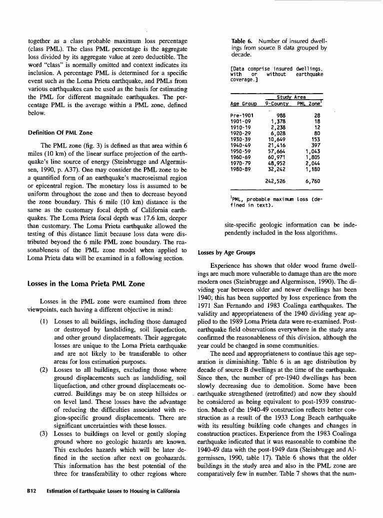
Table 6. Number of insured dwell­ ings from source B data grouped by decade.

[Data comprise insured dwellings, with or without earthquake coverage.]

Study AreaAge Group 9-County PML Zone

28181280

153397

1,0431,8052,0441,180

6,760

Pre-19011901-091910-191920-291930-391940-491950-591960-691970-791980-89

9881,3782,2386,02810,64921,41657,66460,97148,95232,242

242,526

VML, probable maximum loss (de­ fined in text).

site-specific geologic information can be inde­ pendently included in the loss algorithms.

Losses by Age Groups

Experience has shown that older wood frame dwell­ ings are much more vulnerable to damage than are the more modern ones (Steinbrugge and Algermissen, 1990). The di­ viding year between older and newer dwellings has been 1940; this has been supported by loss experience from the 1971 San Fernando and 1983 Coalinga earthquakes. The validity and appropriateness of the 1940 dividing year ap­ plied to the 1989 Loma Prieta data were re-examined. Post- earthquake field observations everywhere in the study area confirmed the reasonableness of this division, although the year could be changed in some communities.

The need and appropriateness to continue this age sep­ aration is diminishing. Table 6 is an age distribution by decade of source B dwellings at the time of the earthquake. Since then, the number of pre-1940 dwellings has been slowly decreasing due to demolition. Some have been earthquake strengthened (retrofitted) and now they should be considered as being equivalent to post-1939 construc­ tion. Much of the 1940-49 construction reflects better con­ struction as a result of the 1933 Long Beach earthquake with its resulting building code changes and changes in construction practices. Experience from the 1983 Coalinga earthquake indicated that it was reasonable to combine the 1940-49 data with the post-1949 data (Steinbrugge and Al­ germissen, 1990, table 17). Table 6 shows that the older buildings in the study area and also in the PML zone are comparatively few in number. Table 7 shows that the num-

B12 Estimation of Earthquake Losses to Housing in California

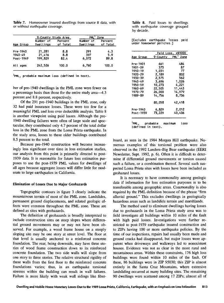
Table 7. Homeowner insured dwellings from source B data, with or without earthquake coverage.

9-County Study Area

Age Group

Pre-1940 1940-49 Post -1949

Number of Dwellings

21,281 21,416 199,829

Percent of Total

8.8 8.8

82.4

PML 1 ZoneNumber of Owe I lings

291 397

6,072

Percent of Total

4.3 5.9

89.8

Table 8. Paid losses to dwellings with earthquake coverage grouped by decade.

[Excludes earthquake losses paid under homeowner policies.]

All ages 242,526 100.0 6,760 100.0

*PML, probable maximum loss (defined in text).

ber of pre-1940 dwellings in the PML zone were fewer on a percentage basis than those for the entire study area 4.3 percent and 8.8 percent, respectively.

Of the 291 pre-1940 buildings in the PML zone, only 32 had paid insurance losses. These were too few for a meaningful PML and loss over deductible analysis. Table 8 is another viewpoint using paid losses. Although the pre- 1940 dwelling failures were often of large scale and spec­ tacular, they contributed only 4.7 percent of the total dollar loss in the PML zone from the Loma Prieta earthquake. In the study area, losses to these older buildings contributed 8.5 percent to the total.

Because pre-1940 construction will become increas­ ingly less significant over time in loss estimation studies, our analysis from this point is primarily directed to post- 1939 data. It is reasonable for future loss estimation pur­ poses to use the post-1939 PML values for dwellings of all ages because aggregate losses will differ little for mod­ erate to large earthquakes in California.

Elimination of Losses Due to Major Geohazards

Topographic contours in figure 3 clearly indicate the mountainous terrain of most of the PML zone. Landslides, permanent ground displacements, and related geologic ef­ fects were common throughout the PML zone. These are defined as sites with geohazards.

The definition of geohazards is broadly interpreted to include construction sites on steep slopes where differen­ tial ground movements may or may not have been ob­ served. For example, a wood frame house on a steeply sloping site may be one story at street level. The floor at that level is usually anchored to a reinforced concrete foundation. The rear, being downside, may have three sto­ ries of wood frame construction down to its reinforced concrete foundation. The two side walls will slope from one story to three stories. The relative structural rigidity of these walls from the first floor to the reinforced concrete foundations varies; thus, in an earthquake torsional stresses within the building can result in wall failures. Failure is more likely with weak wall sidings like fiber-

Age Group

Pre-19011901-091910-191920-291930-391940-491950-591960-691970-791989-89

Paid Loss9- County

661373

1,0312,1892,5753,69610,27322,50526,00014,756

. x$1000PML 1 Zone

4848777

802562

1,0264,22111,44314,9798,736

Pre-1940 Post-1939

80,058

6,82973,229

42,418

2,01240,406

VML, probable (defined in text).

loss

board, as seen in the 1984 Morgan Hill earthquake. Nu­ merous examples of this torsional problem were also observed in the 1992 Landers-Big Bear earthquake (EERI Newsletter, Sept. 1992, p. 6). Often it is difficult to deter­ mine if differential ground movements or torsion caused such a failure, or a combination thereof. Several such sus­ pected Loma Prieta sites with losses have been included as geohazard losses.

It is necessary to have commonality among geologic data if information for loss estimation purposes is to be transferable among geographic areas. Commonality is also required by the PML definition because of the phrase "firm alluvial ground." This excludes dwellings in geologically hazardous areas such as landslide terrain and marshlands.

The method used to eliminate dwellings having losses due to geohazards in the Loma Prieta study area was to field investigate all buildings within 10 miles of the fault with high paid losses. Investigations were further re­ stricted to post-1939 earthquake insured construction and to ZIPs having 100 or more earthquake policies. By the time of our inspections, repairs had usually been made and ground cracks had disappeared, but major losses were ap­ parent when driveways and walkways led to nonexistent houses. Evidence was not as clear in the more rural and mountainous areas. Within these constraints, 176 high loss buildings were found within 10 miles of the fault. Of these, 86 buildings were in ZIP 95030; this ZIP is almost entirely in the Santa Cruz Mountains, where extensive landsliding occurred at many building sites. The remaining 90 dwellings were scattered among 17 ZIPs; almost all of

Dwelling and Mobile Home Monetary Losses Due to the 1989 Loma Prieta, California, Earthquake, with an Emphasis on Loss Estimation B13

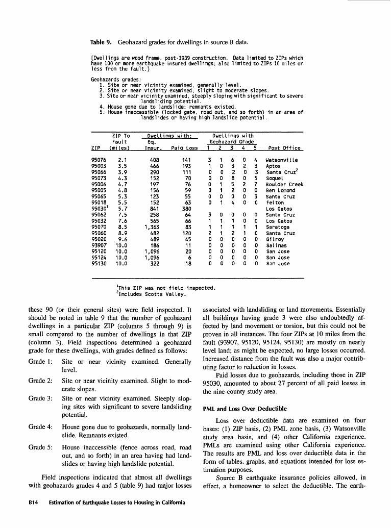
Table 9. Geohazard grades for dwellings in source B data.

[Dwellings are wood frame, ppst-1939 construction. Data limited to ZIPs which have 100 or more earthquake insured dwellings: also limited to ZIPs 10 miles or less from the fault.]

Geohazards grades:1. Site or near vicinity examined, generally level.2. Site or near vicinity examined, slight to moderate slopes.3. Site or near vicinity examined, steeply sloping with significant to severe

landsliding potential.4. House gone due to landslide: remnants existed.5. House inaccessible (locked gate, road out. and so forth) in an area of

landslides or having high landslide potential.

ZIP To Fault

ZIP (miles)

950769500395066950739500695005950659501895030 1950629503295070950609502093907951209512495130

2.13.53.94.34.74.85.35.55.77.57.68.58.99.610.010.010.010.0

Dwellings with:Eq. Insur.

408466290152197156123152841258565

1,363482489186

1,0961,096322

Paid Loss

1411931117076595563

380646683120451120618

Dwellings with Geohazard Grade 12345

31000000

311200000

10001101

011100000

63285204

011200000

02002000

001100000

43357030

001000000

Post Office

UatsonvilleAptosSanta Cruz2SoquelBoulder CreekBen LomondSanta CruzFeltonLos GatosSanta CruzLos GatosSaratogaSanta CruzGilroySalinasSan JoseSan JoseSan Jose

1-rhis ZIP was not field inspected. Includes Scotts Valley.

these 90 (or their general sites) were field inspected. It should be noted in table 9 that the number of geohazard dwellings in a particular ZIP (columns 5 through 9) is small compared to the number of dwellings in that ZIP (column 3). Field inspections determined a geohazard grade for these dwellings, with grades defined as follows:

Grade 1: Site or near vicinity examined. Generally level.

Grade 2: Site or near vicinity examined. Slight to mod­ erate slopes.

Grade 3: Site or near vicinity examined. Steeply slop­ ing sites with significant to severe landsliding potential.

Grade 4: House gone due to geohazards, normally land­ slide. Remnants existed.

Grade 5: House inaccessible (fence across road, road out, and so forth) in an area having had land­ slides or having high landslide potential.

Field inspections indicated that almost all dwellings with geohazards grades 4 and 5 (table 9) had major losses

associated with landsliding or land movements. Essentially all buildings having grade 3 were also undoubtedly af­ fected by land movement or torsion, but this could not be proven in all instances. The four ZIPs at 10 miles from the fault (93907, 95120, 95124, 95130) are mostly on nearly level land; as might be expected, no large losses occurred. Increased distance from the fault was also a major contrib­ uting factor to reduction in losses.

Paid losses due to geohazards, including those in ZIP 95030, amounted to about 27 percent of all paid losses in the nine-county study area.

PML and Loss Over Deductible

Loss over deductible data are examined on four bases: (1) ZIP basis, (2) PML zone basis, (3) Watsonville study area basis, and (4) other California experience. PMLs are examined using other California experience. The results are PML and loss over deductible data in the form of tables, graphs, and equations intended for loss es­ timation purposes.

Source B earthquake insurance policies allowed, in effect, a homeowner to select the deductible. The earth-

B14 Estimation of Earthquake Losses to Housing in California

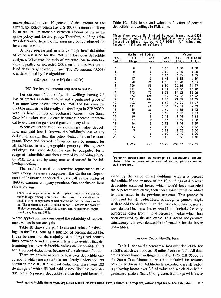
quake deductible was 10 percent of the amount of the earthquake policy which has a $100,000 minimum. There is no required relationship between amount of the earth­ quake policy and the fire policy. Therefore, building value was determined from the fire insurance policy adjusted for insurance to value.

A more precise and restrictive "high loss" definition of value was used for the PML and loss over deductible analyses. Whenever the ratio of structure loss to structure value equalled or exceeded 2/3, then this loss "was corre­ lated with its geohazard, if any. The 2/3 amount (0.667) was determined by the algorithm:

(EQ paid loss + EQ deductible)

(HO fire insured amount adjusted to value).

For purpose of this study, all dwellings having 2/3 loss or greater as defined above and a geohazard grade of 3 or more were deleted from the PML and loss over de­ ductible analysis. Additionally, all dwellings in ZIP 95030, with its large number of geohazard losses in the Santa Cruz Mountains, were deleted because it became impracti­ cal to evaluate the geohazard grade at many sites.

Whenever information on a building's value, deduct­ ible, and paid loss is known, the building's loss at any deductible greater than the policy deductible can be com­ puted. These and derived information may be summed for all buildings in any geographic grouping. Finally, each building's loss over deductible can be computed for a range of deductibles and then summed by individual ZIPs, by PML zone, and by study area as discussed in the fol­ lowing sections.

The methods used to determine replacement value vary among insurance companies. The California Depart­ ment of Insurance conducted a data call in the winter of 1993 to examine company practices. One conclusion from this study was:

There is a large variation in the replacement cost calculation methodology among companies. This results in variations as much as 50% in replacement cost calculations for the same dwell­ ing. The replacement cost formulas do not..... address the costs of hillside construction. (California Department of Insurance, unpub­ lished data, January, 1994).

Where applicable, we considered the reliability of replace­ ment values in our analysis.

Table 10 shows the paid losses and values for dwell­ ings in the PML zone as a function of percent deductible. It can be seen that the majority of buildings had deduct­ ibles between 5 and 11 percent. It is also evident that de­ termining loss over deductible values are impossible for 0 and 1 percent deductibles because of the absence of data.

There are several aspects of loss over deductible cal­ culations which are sometimes not clearly understood. As shown in table 10, at 5 percent deductible, there were 100 dwellings of which 53 had paid losses. The loss over de­ ductible at 5 percent deductible is thus the paid losses di-

Table 10. Paid losses and values as function of percent deductible for dwellings in PML zone.

[Data from source B; limited to wood frame, post-1939 construction and to ZIPs which had 10 or more earthquake insured buildings, excluding ZIP 95030. All values and losses in millions of dollars.]

Number of Bldgs.Pet. Ded. 1

01234567891011121314151617181920

All Bldqs.

001

1740100131173273491293131857849271613915

1,933

Paid Loss

0019

28537275126204914030148932101

767

Paid Loss

0.000.000.031.461.521.891.311.712.353.301.440.360.340.150.180.130.030.020.010.000.00

16.22

ValueAll Bldgs.

0.000.000.556.8810.7820.5623.1827.6339.2272.3940.7414.319.867.505.162.851.460.991.030.100.36

285.53

Paid Loss Bldgs.

0.000.000.554.397.8311.1712.4812.0617.9230.4511.974.323.131.330.611.080.290.120.060.000.10

119.85

Percent deductible is average of earthquake dollar deductible in terms of percent of value, plus or minus 0.5 percent.

vided by the value of all buildings with a 5 percent deductible. If one or more of the 40 buildings at 4 percent deductible sustained losses which would have exceeded the 5 percent deductible, then these losses must be added to those stated in the previous sentence. This process is continued for all deductibles. Although a person might wish to add the deductible to the losses to obtain losses at zero deductible, these losses would not include the very numerous losses from 1 to 4 percent of value which had been excluded by the deductible. This would not produce satisfactory loss over deductible information for the lower deductibles.

Loss Over Deductible Zip Basis

Table 11 shows the percentage loss over deductible for all ZIPs which are not over 10 miles from the fault. All data are on wood frame dwellings built after 1939. ZIP 95030 in the Santa Cruz Mountains was not included for reasons previously discussed. Additionally excluded were all build­ ings having losses over 2/3 of value and which also had a geohazard grade 3 (table 9) or greater. Buildings with lower

Dwelling and Mobile Home Monetary Losses Due to the 1989 Loma Prieta, California, Earthquake, with an Emphasis on Loss Estimation B15

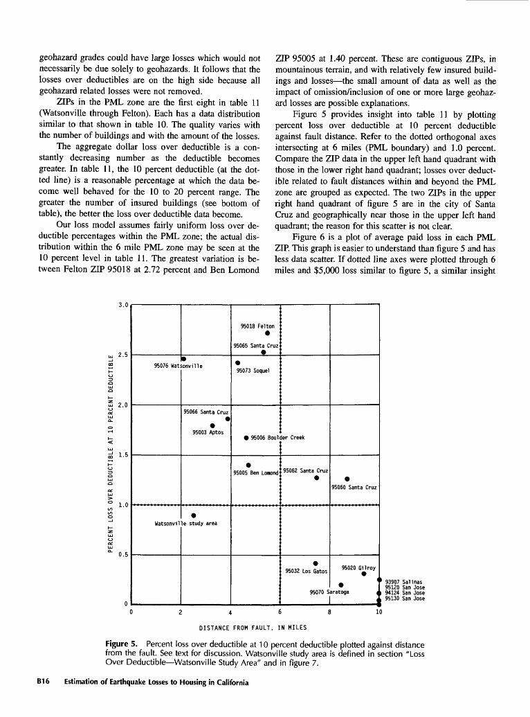
geohazard grades could have large losses which would not necessarily be due solely to geohazards. It follows that the losses over deductibles are on the high side because all geohazard related losses were not removed.

ZIPs in the PML zone are the first eight in table 11 (Watsonville through Felton). Each has a data distribution similar to that shown in table 10. The quality varies with the number of buildings and with the amount of the losses.

The aggregate dollar loss over deductible is a con­ stantly decreasing number as the deductible becomes greater. In table 11, the 10 percent deductible (at the dot­ ted line) is a reasonable percentage at which the data be­ come well behaved for the 10 to 20 percent range. The greater the number of insured buildings (see bottom of table), the better the loss over deductible data become.

Our loss model assumes fairly uniform loss over de­ ductible percentages within the PML zone; the actual dis­ tribution within the 6 mile PML zone may be seen at the 10 percent level in table 11. The greatest variation is be­ tween Felton ZIP 95018 at 2.72 percent and Ben Lomond

ZIP 95005 at 1.40 percent. These are contiguous ZIPs, in mountainous terrain, and with relatively few insured build­ ings and losses the small amount of data as well as the impact of omission/inclusion of one or more large geohaz­ ard losses are possible explanations.

Figure 5 provides insight into table 11 by plotting percent loss over deductible at 10 percent deductible against fault distance. Refer to the dotted orthogonal axes intersecting at 6 miles (PML boundary) and 1.0 percent. Compare the ZIP data in the upper left hand quadrant with those in the lower right hand quadrant; losses over deduct­ ible related to fault distances within and beyond the PML zone are grouped as expected. The two ZIPs in the upper right hand quadrant of figure 5 are in the city of Santa Cruz and geographically near those in the upper left hand quadrant; the reason for this scatter is not clear.

Figure 6 is a plot of average paid loss in each PML ZIP. This graph is easier to understand than figure 5 and has less data scatter. If dotted line axes were plotted through 6 miles and $5,000 loss similar to figure 5, a similar insight

3.0

2.5

2.0

1.5

1.0

0.5

95076 Wat

Watsonvil

sonville

95066 Santa Cruz

95003 Aptos

le study area

95018 Felton

95065 Santa Cruz

95073 Soquel

95006 Boul

95005 Ben Lomond

ler Creek

95062 Santa Cruz

95032 Los Gatos

95070 S

95060 Santa Cruz

95020 Gilroy

<

aratoga J

93907 Salinas 95120 San Jose 94124 San Jose 95130 San Jose

10

DISTANCE FROM FAULT, IN MILES

Figure 5. Percent loss over deductible at 10 percent deductible plotted against distance from the fault. See text for discussion. Watsonville study area is defined in section "Loss Over Deductible Watsonville Study Area" and in figure 7.

B16 Estimation of Earthquake Losses to Housing in California

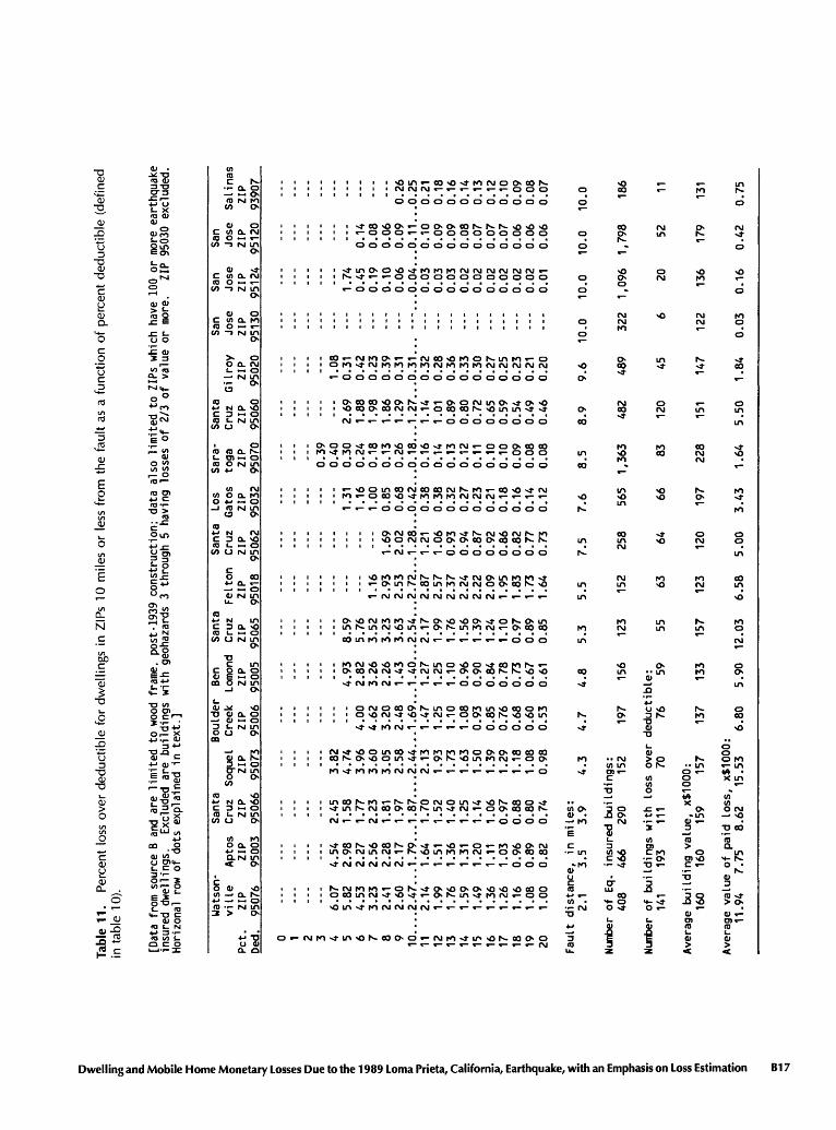
Tabl

e 11

. P

erce

nt l

oss

ove

r deduct

ible

for

dw

elli

ng

s in

ZIP

s 10

mile

s or

less

fro

m t

he f

au

lt as

a f

unct

ion o

f pe

rcen

t deduct

ible

(de

fined

in

tab

le 1

0).

n BL a: I. o

[Dat

a fro

m s

ourc

e B

and

are

limite

d t

o w

ood

fram

e,

post

-193

9 co

nst

ruct

ion

; da

ta

also

lim

ited t

o Z

IPs

whi

ch h

ave

100

or m

ore

eart

hqua

ke

insu

red

dwel

lings

. E

xclu

ded

are

build

ings

with

ge

ohaz

ards

3

thro

ugh

5 ha

ving

lo

sses

of

2/3

of

valu

e or

m

ore.

ZI

P

9503

0 ex

clud

ed.

Hor

i zon

al

row

of

dots

exp

lain

ed i

n t

ext.

]

Wats

on-

Sant

avi

lle

Apto

s Cr

uz

Soqu

elPet.

ZIP

ZIP

ZIP

ZIP

Ded.

9507

6 95

003

9506

6 95

073

0 1 2 3 4 6.07

4.54

2.

45

3.82

5 5.

82

2.98

1.

58

4.74

6 4.

53

2.27

1.

77

3.96

7 3.

23

2.56

2.

23

3.60

8 2.41

2.28

1.81

3.05

9 2.

60

2.17

1.97

2.58

10.... 2. 4

7...

1.79... 1.8

7...

. 2.

44.

11

2.14

1.64

1.70

2.

1312

1.99

1.51

1.52

1.

9313

1.76

1.

36

1.40

1.

7314

1.59

1.

31

1.25

1.63

15

1.49

1.

20

1.14

1.

5016

1.

36

1.11

1.06

1.

3917

1.

26

1.03

0.97

1.29

18

1.16

0.

96

0.88

1.18

19

1.08

0.89

0.80

1.

0820

1.

00

0.82

0.

74

0.98

Faul

t di

stan

ce,

in m

iles

:2.

1 3.

5 3.9

4.3

Numb

er of

Eq

. in

sure

d buildings:

408

466

290

152

Numb

er of bu

ildi

ngs

with

loss ov

er14

1 193

111

70

Average

building v

alue

, x$1000:

160

160

159

157

Average

valu

e of

paid lo

ss,

x$1000

11.94

7.75

8.62

15.5

3

Boulder

Cree

kZI

P95006

...

4.00

4.62

3.20

2.48

..1.

69.

1.47

1.25

1.10

1.08

0.93

0.85

0.76

0.68

0.60

0.53

4.7 197

Ben

Lomond

ZIP

9500

5

4.93

2.82

3.26

2.26

1.43

..1.40..

1.27

1.25

1.10

0.96

0.90

0.84

0.78

0.73

0.67

0.61

4.8 156

Sant

aCr

uzZI

P95

065

8.59

5.76

3.52

3.23

3.63

.2.54.

2.17

1.99

1.76

1.56

1.39

1.24

1.10

0.97

0.89

0.85

5.3 123

Felt

onZI

P95018

...

...

1.16

2.93

2.53

..2.72..

2.87

2.57

2.37

2.24

2.22

2.09

1.95

1.83

1.73

1.64

5.5 152

Sant

aCr

uzZIP

95062

-..

...

...

1.69

2.02

.1.28..

1.21

1.06

0.93

0.94

0.87

0.92

0.86

0.82

0.77

0.73

7.5 258

Los

Gato

sZI

P95032

1.31

1.16

1.00

0.85

0.68

.0.42.

0.38

0.38

0.32

0.27

0.23

0.21

0.18

0.16

0.14

0.12

7.6 565

Sara

­to

ga ZIP

95070

0.39

0.40

0.30

0.24

0.18

0.13

0.26

..0.

18.

0.16

0.14

0.13

0.12

0.11

0.10

0.10

0.09

0.08

0.08

8.5

1,363

Sant

aCr

uz ZIP

9506

0

2.69

1.88

1.98

1.86

1.29

..1.

27.

1.14

1.01

0.89

0.80

0.72

0.65

0.59

0.54

0.49

0.46

8.9 482

Gi Iro

yZI

P95

020

1 flA

I . DO

0.31

0.42

0.23

0.39

0.31

..0.31.

0.32

0.28

0.36

0.33

0.30

0.27

0.25

0.23

0.21

0.20

9.6 489

San

San

Jose

Jo

seZIP

ZIP

9513

0 95124

---

1.74

---

0.45

---

0.19

---

0.10

---

0.06

.. --

-...

0.04

.---

0.03

---

0.03

---

0.03

---

0.02

---

0.02

0.02

---

0.02

---

0.02

---

0.02

---

0.01

10.0

10

.0

322

1,09

6

San

Jose

ZIP

95120

...

0.14

0.08

0.06

0.09

..0.11.

0.10

0.09

0.09

0.08

0.07

0.07

0.07

0.06

0.06

0.06

10.0

1,79

8

Sali

nas

ZIP

93907

...

...

-..

...

0.26

..0.25

0.21

0.18

0.16

0.14

0.13

0.12

0.10

0.09

0.08

0.07

10.0 18

6

deductible:

76 137

J

6.80

59 133

5.90

55 157

12.0

3

63 123

6.58

64 120

5.00

66 197

3.43

83 228

1.64

120

151

5.50

45 147

1.84

6 20

122

136

0.03

0.16

52 179

0.42

11 131

0.75

would develop. Figure 5 is more informative since it in­ cludes deductibles and therefore eliminates a variable. The Watsonville study area, by itself in the lower left hand quadrant in both figures, will be discussed in the next sec­ tion. Loss attenuation within the PML zone is not evident, although one could draw a line or curve through the entire 10 mile data set.

The variation in loss over deductible amounts among ZIPs may be partially attributed to construction: the number of stories, type of roof (wood, tile), masonry chimneys (or none), interior finishes, and the like. The influence of some of these construction components will be discussed later. Most probably of greater importance are geophysical fac­ tors: fault distance, directionality of seismic waves from their source, and building sites susceptible to geohazards.

The effect of geohazards on loss over deductible is shown in table 12. The effect on individual ZIPs varies from 7 to 52 percent. The reduction is 23 percent in the PML zone and is 21 percent in the 10 mile zone. The small percentage difference is due to the few losses over 10 percent beyond the PML zone 45 to 48 buildings, re­ spectively. ZIP 95030 is excluded.

Loss Over Deductible Zone Basis

The information in table 11 is shown in aggregate form in columns 3 and 4 of table 13. The dots at 10 per­ cent deductible have the same sense as those in table 11. The loss over deductibles in columns 2, 3, and 4 are better behaved at lower deductibles than those for individual

ZIPs in table 11 owing to the larger data set of buildings and losses. The PML zone values in column 3 appear rea­ sonable beyond the 5 percent deductible (table 10).

The effect of geohazard elimination in the PML zone is significant; compare columns 2 and 3 at 10 percent de­ ductible. The effect of distance on loss is also significant; compare columns 3 and 4.

The 1983 Coalinga data shown here are for informa­ tional purposes and will be discussed below under "Other California Experience."

Loss Over Deductible Watsonville Study Area Basis

It has been stated that the elimination of grade 3 and higher geohazard buildings with high losses undoubtedly discounted an unknown number of losses from buildings with lessor or undetected geohazards. This undoubtedly in­ creased the loss over deductible values for ZIPs in table 11 and for the PML zone in column 3 of table 13. It was therefore desirable to examine a test area where a better examination of the influence of geohazards on losses could be undertaken.

The City of Watsonville and the contiguous portions of the community of Freedom to the northwest were cho­ sen for a detailed study (fig. 7). This study area consists of a small area surrounded by ZIP 95076 (fig. 4). Watsonville is the largest city entirely within the PML zone and also the closest large one to the faulting. The study area is mostly on level or gently sloping terrain. The principal ex­ ception is Struve Slough, where potential geohazards were

$20.000

$15,000

$10,000

$5,000

$0

95076 W

Watsonvllle

itsonville

95003 Aptos *

95006 Boulder <

95005 Ben

study area

95073 Soquel

95065 Santa Cruz

95066 Santa Cruz

95018 F >eek

.omond

>1ton

95062 Santa Cruz

95032 Los Gatos

95070 S

95060 Santa Cruz

95020 Gilroy

Varatoga I

93907 Sallnas 95120 San Jose 94124 San Jose 95130 San Jose

4 6

DISTANCE FROM FAULT, IN MILES

10

Figure 6. Average paid building loss per earthquake insured building plotted against distance from fault. See text for discussion.

B18 Estimation of Earthquake Losses to Housing in California

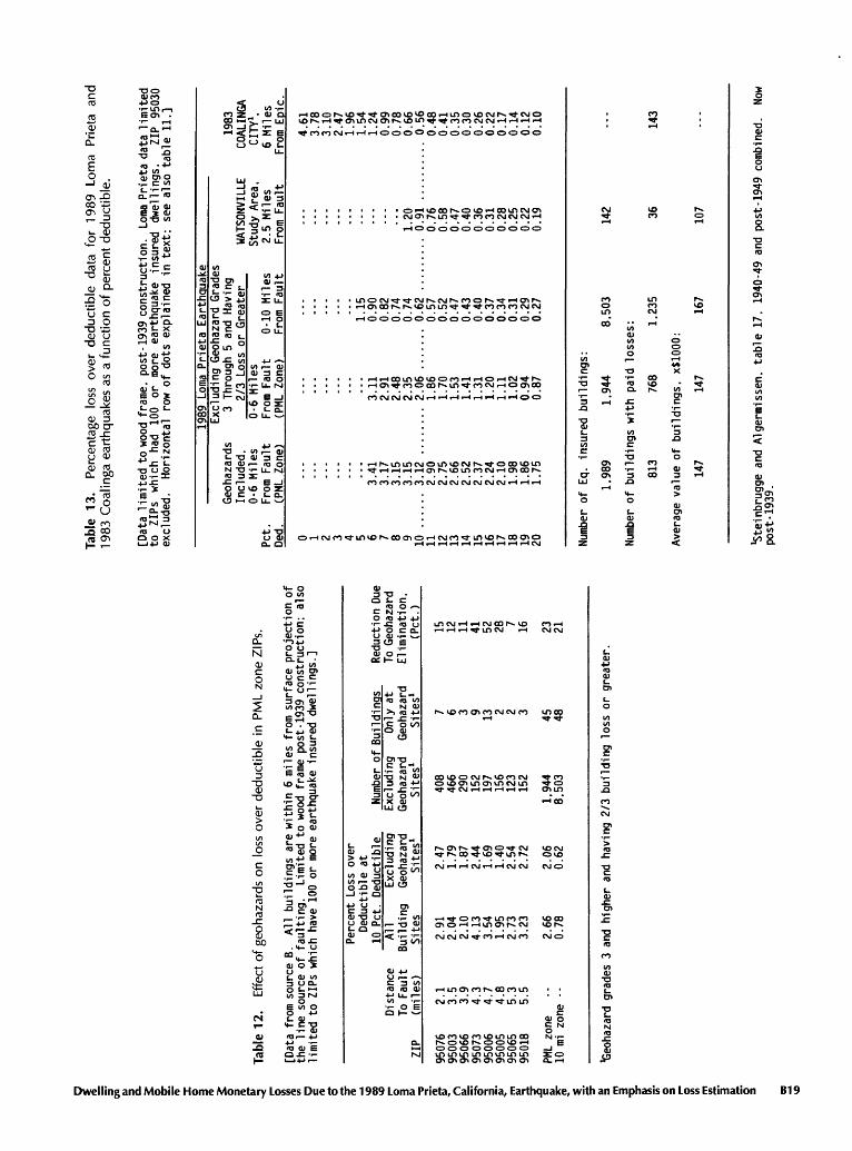
Tab

le

13.

Per

cent

age

loss

o

ver

de

du

ctib

le

data

fo

r 1989

Lom

a P

rieta

a

nd

1983 C

oa

ling

a e

art

hquake

s as

a f

un

ctio

n o

f p

erc

en

t d

ed

uct

ible

.

Q. i CT

ffi" I n O I

[Dat

a lim

ited t

o w

ood

fram

e,

post

-193

9 co

nst

ruct

ion

. Lo

ma

Prie

ta d

ata

limited

to

ZIP

s w

hich

ha

d 10

0 o

r m

ore

eart

hqua

ke

insu

red

dw

elli

ng

s.

ZIP

95

030

exc

lud

ed

. H

orizo

nta

l ro

w o

f dots

e

xpla

ine

d in

text:

se

e als

o ta

ble

11.]

o S-

a n SL

f .a

I

Tabl

e 12

. E

ffect

of

geohaza

rds

on

los

s o

ver

deduct

ible

in

PM

L zo

ne Z

IPs.

[Dat

a fr

om s

ourc

e B.

A

ll build

ings

are

within

6 m

iles

from

surf

ace

pro

ject

ion o

f th

e l

ine

sou

rce

of

faultin

g.

Lim

ited t

o w

ood

fram

e po

st-1

939

con

stru

ctio

n;

als

o

limite

d t

o

ZIP

s w

hich

ha

ve

100

or

mor

e ea

rthq

uake

in

sure

d d

we

llin

gs.]

Perc

ent

Loss o

ver

Dedu

ctib

le a

t

ZIP

95076

9500

39506

695

073

95006

9500

595

065

95018

Dist

ance

To F

ault

(miles)

2.1

3.5

3.9

4.3

4.7

4.8

5.3

5.5

PML

zone

- -

10 m

izone

10 P

et.

All

Building

Site

s

2.91

2.04

2.10

4.13

3.54

1.95

2.73

3.23

2.66

0.78

Deductible

Excl

udi n

gGeohazard

Sites1

2.47

1.79

1.87

2.44

1.69

1.40

2.54

2.72

2.06

0.62

Numb

er o

fExcludin

gGeohazar

dSites1

408

466

290

152

197

156

123

152

1.944

8.50

3

Buil

ding

sOnly a

tGeohazard

Sites1

7 6 3 9 13 2 2 3 45 48

Reduction

Due

To Geo

haza

rdElimination.

(Pet

.)

15 12 11 41 52 28 7 16 23 21

"Geo

haza

rd g

rade

s 3

and

hig

her

and

havi

ng 2

/3 b

uild

ing l

oss

or

gre

ate

r.

1989 L

oma

Prie

ta E

arth

quak

eExclud

ing

Geoh

azar

d Gr

ades

Pet.

Ded. 0 1 2 3 4 5 6 7 8 9 10 11 12 13 14 15 16 17 18 19 20

Geoh

azar

dsIncluded.

0-6

Mile

sFrom F

ault

(PML Z

one)

...

...

3.41

3.17

3.15

3.15

....

3.12 ..

..2.90

2.75

2.66

2.52

2.37

2.24

2.10

1.98

1.86

1.75

3 Th

rough

2/3

Loss

0-6

Miles

From

Fau

lt(PML Z

one)

...

...

3.11

2.91

2.48

2.35

....

2.06 ...

1.86

1.70

1.53

1.41

1.31

1.20

1.11

1.02

0.94

0.87

5 an

d Having

or G

reat

er

0-10 M

iles

From F

ault

...

1.15

0.90

0.82

0.74

0.74

.... 0.62 .....

0.57

0.52

0.47

0.43

0.40

0.37

0.34

0.31

0.29

0.27

WATS

ONVI

LLE

Study

Area,

2.5

Miles

From F

ault

...

...

...

1.20

.... 0.91 ......

0.76

0.58

0.47

0.40

0.36

0.31

0.28

0.25

0.22

0.19

1983

COAL

INGA

CITY

1.6

Miles

From E

pic.

4.61

3.78

3.10

2.47

1.96

1.54

1.24

0.99

0.78

0.66

.,,, 0.56

0.48

0.41

0.35

0.30

0.26

0.22

0.17

0.14

0.12

0.10

Num

ber

of

Eq.

in

sure

d b

uild

ing

s:

1.98

9 1.

944

8.50

3

Num

ber

of

bu

ildin

gs w

ith

paid

lo

sse

s:

813

768

1.23

5

Ave

rage

va

lue

of

bu

ildin

gs.

x$10

00:

147

147

167

142 36 107

143

*Ste

inbr

ugge

and

Alg

erm

isse

n.

tab

le

17.

1940

-49

and

post

-194

9 co

mbi

ned.

p

ost

-19

39

.No

w

Figure 7. Watsonville study area and Watsonville city limits. Solid triangles are locations of mobile home parks; park numbers are identified in table 26. Open circles are structures outside of the central business district posted as hazardous after the earthquake.

B20 Estimation of Earthquake Losses to Housing in California

found on hillsides and bottomland. This area has been de­ veloped in recent years, and most structures were expected to have had some geotechnical advice on foundations.

The study area is compact, about 3.5 miles long by 1.5 miles wide. The surface projection of the modeled earthquake's line source of seismic energy is shown in fig­ ure 7 (see also figs. 2 and 3). The centroid of all dwellings in the study area is about 2.5 miles from the surface pro­ jection of the line source. The quality of the dwelling dis­ tances from this line source must be understood in the limitations of the fault model.

Most housing in the study area is of post-1939 construc­ tion. The 1940 census states 2,829 one to four family units in Watsonville city; the 1990 census states 7,371. This repre­ sents over 250 percent growth due to post-1939 construction.

The open circles in figure 7 represent structures posted by inspectors immediately after the earthquake as "unsafe" based on the Applied Technology Council Field Manual (1989). The open circles were plotted from an unpublished City of Watsonville manuscript map which summarized the inspectors' postings. We excluded postings in the central business district and at several large industrial structures. As a result, the open circles normally represent wood frame dwellings when not located on the main thoroughfares named in figure 7. Open circles along these thoroughfares can be mercantile buildings of other than wood frame con­ struction as well as wood frame dwellings. The "unsafe" structures were almost always of pre-1940 construction. City hall maps showing land annexations through 1930 in­ dicated that about 75 percent of the open circle structures fell within the original city limits and these annexations. By strong contrast, the modern wood frame dwellings in the southeast section of the city had no posted "unsafe" dwell­ ings. Many of these dwellings had concrete first floor slabs on grade and therefore did not have cripple wood studs supporting the first floor. Soil conditions in this south­ eastern section of Watsonville were soft alluvial materials appearing to be similar to those where high density damage was noted. Another possible soil indicator is the mapped 100 year flood limit, which may be roughly described as somewhat south of West Beach Street on fig. 7 and its northeasterly extension to the city limits.

The other newer areas of Watsonville to the northwest are on higher ground and construction is newer. Here posted "unsafe" buildings were few.

Available evidence indicates that dwelling age was the principal criteria for differences in dwelling damage and loss patterns.

In table 14, the loss over deductible at 10 percent de­ ductible for the Watsonville study area may be compared using information from tables 11 and 12. Field inspections to identify geohazard sites were made of the post-1939 dwellings in the hill areas, including those around Struve Slough (fig. 7). The highest predeductible loss was 43.5

Table 14. Loss over deductible com­ parisons at 10 percent deductible.

Loss Over Deductible, in Percent

Watsonville study area 0.91Watsonville ZIP 95076 2.47PML zone 2.06

percent, with all others being substantially less. Some losses may have been associated with cuts and fills be­ neath dwellings, but no sites exceeded geohazard grade 2. The study area is surrounded by Watsonville ZIP 95076 with higher losses. Construction practices and quality were not reasonable explanations for the large differences. Seis­ mic explanations will be later discussed in "PMLs and Equations for Loss Over Deductible."

Loss Over Deductible Other California Experience

The major importance of other California experience is that it provides loss over deductible information down to zero deductible, which is not available for Loma Prieta.

Table 13 information on the 1983 Coalinga earth­ quake is from table 17 of Steinbrugge and Algermissen (1990), revised to combine 1940-49 construction with that for post-1949 construction. This revision was for data compatibility purposes.

All further references to tables, figures, and curves in this section are to Steinbrugge and Algermissen (1990), except where otherwise stated. Information from their table 17 is shown graphically as curve 3 in their figure 4. "Curve 3 in figure 4 was considered to be the most useful for loss over deductible applications" (p. A42). Fortu­ nately, the data source for this curve is the same as that for Loma Prieta source B, thereby eliminating most inconsis­ tencies among insurance company loss adjusting practices.

We re-examined the choice of curve 3 among those shown in their figure 4. The following comparisons are made at zero loss over deductible for "post-49" buildings with "wood or concrete floors." The 6.60 percent for curve 4 compared to 4.29 percent for curve 3 is due to the changes in building values since all other data were the same. Building values for curve 4 were determined by two local realtors working independently. They determined av­ erage pre-earthquake market values on a city block-by- block basis, or by a group of blocks in some instances. The paid insurance losses are more realistic than the real­ tors' estimates based on groups of houses.

Curve 2 at 8.78 percent is the highest of the three for Coalinga. Half of this increase from curve 3 of 4.29 to 8.78 percent may be due to differences in building valua­ tion methods discussed in the previous paragraph. The other half may be due to uncertainties in the numerical

Dwelling and Mobile Home Monetary Losses Due to the 1989 Loma Prieta, California, Earthquake, with an Emphasis on Loss Estimation B21

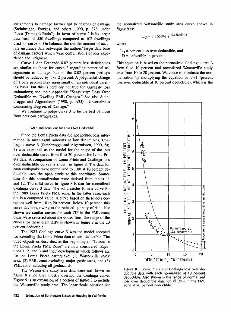
assignments to damage factors and to degrees of damage (Steinbrugge, Fowkes, and others, 1990, p. 373, under "Loss (Damage) Ratio"). In favor of curve 2 is its larger data base of 530 dwellings compared to 102 dwellings used for curve 3. On balance, the smaller amount of accu­ rate insurance data outweighs the authors' larger data base of damage factors which were combinations of loss expe­ rience and judgment.

Curve 1 San Fernando 8.02 percent loss deficiencies are similar to those for curve 2 regarding numerical as­ signments to damage factors; the 8.02 percent perhaps should be reduced by 1 or 2 percent. A judgmental change of 1 or 2 percent may seem small on an individual dwell­ ing basis, but this is certainly not true for aggregate loss estimations; see their Appendix "Sensitivity: Loss Over Deductible vs. Dwelling PML Changes." See also Stein­ brugge and Algermissen (1990, p. A35), "Uncertainties Concerning Degrees of Damage."

We continue to judge curve 3 to be the best of those from previous earthquakes.

PMLS and Equations for Loss Over Deductible

Since the Loma Prieta data did not include loss infor­ mation in meaningful amounts at low deductibles, Coa- linga's curve 3 (Steinbrugge and Algermissen, 1990, fig. 4) was examined as the model for the shape of the loss over deductible curve from 0 to 20 percent for Loma Pri­ eta data. A comparison of Loma Prieta and Coalinga loss over deductible curves is shown in figure 8. The data for each earthquake were normalized to 1.00 at 10 percent de­ ductible see the open circle at this coordinate. Source data for this normalization were derived from tables 11 and 12. The solid curve in figure 8 is that for normalized Coalinga curve 3 data. The solid circles form a curve for the 1989 Loma Prieta PML zone. In the latter case, each dot is a computed value. A curve based on these dots cor­ relates well from 10 to 20 percent. Below 10 percent, this curve deviates, owing to the reduced quantity of data. Not shown are similar curves for each ZIP in the PML zone; these were centered about the dotted line. The range of the curves for these eight ZIPs is shown in figure 8 at the 20 percent deductible.

The 1983 Coalinga curve 3 was the model accepted for extending the Loma Prieta data to zero deductible. The three objectives described at the beginning of "Losses in the Loma Prieta PML Zone" are now considered. Equa­ tions 1, 2, and 3 and their development which follows are for the Loma Prieta earthquake: (1) Watsonville study area, (2) PML zone excluding major geohazards, and (3) PML zone including all geohazards.

The Watsonville study area data were not shown on figure 8 since they mostly overlaid the Coalinga curve. Figure 9 is an expansion of a portion of figure 8 to include the Watsonville study area. The logarithmic equation for

the normalized Watsonville study area curve shown in figure 9 is:

LD -7.165841 e-°' 188469D

where

LD = percent loss over deductible, and D = deductible in percent.

This equation is based on the normalized Coalinga curve 3 from 0 to 10 percent and normalized Watsonville study area from 10 to 20 percent. We chose to eliminate the nor­ malization by multiplying the equation by 0.91 (percent loss over deductible at 10 percent deductible), which is the

>£° K 3

£§

cc. o

Normalized at 10* deductible

ac.

1

0 5 10 15 20

DEDUCTIBLE, IN PERCENT

Figure 8. Loma Prieta and Coalinga loss over de­ ductible data with each normalized at 10 percent deductible. Also shown is the range of normalized loss over deductible data for all ZIPs in the PML zone at 20 percent deductible.

B22 Estimation of Earthquake Losses to Housing in California

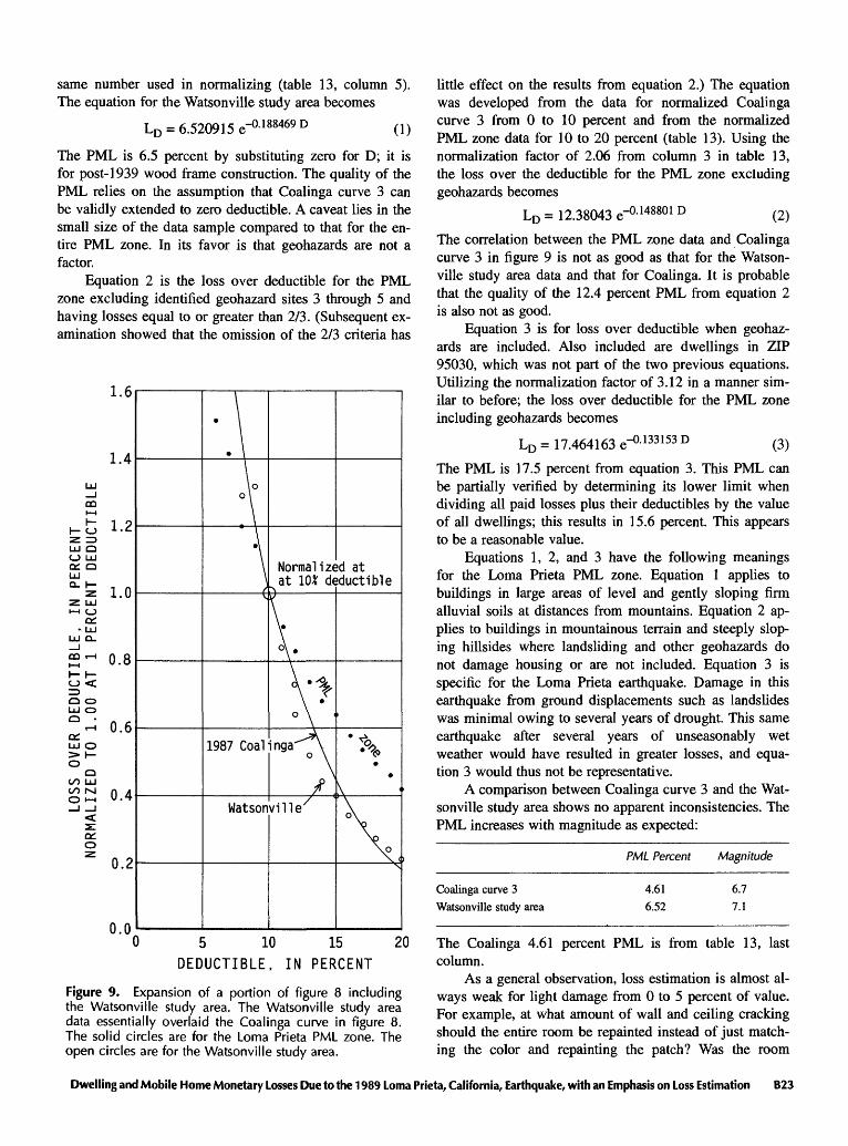
same number used in normalizing (table 13, column 5). The equation for the Watsonville study area becomes

LD = 6.520915 e-°' 188469D (1)

The PML is 6.5 percent by substituting zero for D; it is for post-1939 wood frame construction. The quality of the PML relies on the assumption that Coalinga curve 3 can be validly extended to zero deductible. A caveat lies in the small size of the data sample compared to that for the en­ tire PML zone. In its favor is that geohazards are not a factor.

Equation 2 is the loss over deductible for the PML zone excluding identified geohazard sites 3 through 5 and having losses equal to or greater than 2/3. (Subsequent ex­ amination showed that the omission of the 2/3 criteria has

CO

O

UJ Q O UJ

LUQ. h-

UJ Q-_lCD i I i ih- h- O < ^Q O UJ O Q

T-H

C£UJ O > h- OO

UO UJ GO M O M

Normalized at at 10* deductible

5 10 15 20 DEDUCTIBLE, IN PERCENT

Figure 9. Expansion of a portion of figure 8 including the Watsonville study area. The Watsonville study area data essentially overlaid the Coalinga curve in figure 8. The solid circles are for the Loma Prieta PML zone. The open circles are for the Watsonville study area.

little effect on the results from equation 2.) The equation was developed from the data for normalized Coalinga curve 3 from 0 to 10 percent and from the normalized PML zone data for 10 to 20 percent (table 13). Using the normalization factor of 2.06 from column 3 in table 13, the loss over the deductible for the PML zone excluding geohazards becomes

LD = 12.38043 e.-0.148801 D (2)

The correlation between the PML zone data and Coalinga curve 3 in figure 9 is not as good as that for the Watson­ ville study area data and that for Coalinga. It is probable that the quality of the 12.4 percent PML from equation 2 is also not as good.

Equation 3 is for loss over deductible when geohaz­ ards are included. Also included are dwellings in ZIP 95030, which was not part of the two previous equations. Utilizing the normalization factor of 3.12 in a manner sim­ ilar to before; the loss over deductible for the PML zone including geohazards becomes

LD = 17.464163 e-°' 133153D (3)

The PML is 17.5 percent from equation 3. This PML can be partially verified by determining its lower limit when dividing all paid losses plus their deductibles by the value of all dwellings; this results in 15.6 percent. This appears to be a reasonable value.

Equations 1, 2, and 3 have the following meanings for the Loma Prieta PML zone. Equation 1 applies to buildings in large areas of level and gently sloping firm alluvial soils at distances from mountains. Equation 2 ap­ plies to buildings in mountainous terrain and steeply slop­ ing hillsides where landsliding and other geohazards do not damage housing or are not included. Equation 3 is specific for the Loma Prieta earthquake. Damage in this earthquake from ground displacements such as landslides was minimal owing to several years of drought. This same earthquake after several years of unseasonably wet weather would have resulted in greater losses, and equa­ tion 3 would thus not be representative.

A comparison between Coalinga curve 3 and the Wat­ sonville study area shows no apparent inconsistencies. The PML increases with magnitude as expected:

PML Percent Magnitude

Coalinga curve 3

Watsonville study area

4.61

6.52

6.7

7.1

The Coalinga 4.61 percent PML is from table 13, last column.

As a general observation, loss estimation is almost al­ ways weak for light damage from 0 to 5 percent of value. For example, at what amount of wall and ceiling cracking should the entire room be repainted instead of just match­ ing the color and repainting the patch? Was the room

Dwelling and Mobile Home Monetary Losses Due to the 1989 Loma Prieta, California, Earthquake, with an Emphasis on Loss Estimation B23

badly in need of repainting before the event and if so, should its depreciated value be considered? Parallels exist with a new or old automobile receiving a small dent of unknown origin in the case of no deductible. The amount of the loss as viewed by the owner is often based on who is going to pay the loss. Practices differ among insurance companies with respect to dwellings, but often depreciated value is not considered for repainting purposes.

Size of the PML Zone

Loma Prieta Earthquake

As seen from figures 5 and 6, the 6-mile limit to the PML zone for the Loma Prieta event is a reasonable value. Guidelines for damage attenuation within the PML zone are difficult to ascertain because of ambiguous data. For the present it remains reasonable to use a simplistic aver­ age value for the PML zone.

Smaller Magnitude Earthquakes

Studies of instrumental data (Cloud and Perez, 1967) from the 1966 Parkfield, California, earthquake provide in­ sights into the PML zone boundary. The earthquake's magnitude was about 5.5, and surface faulting was ob­ served. Five accelerograms were obtained within 10 miles of the trace of the San Andreas fault. Cloud and Perez (1967, fig. 10) suggested no reduction in the acceleration from the observed fault trace to 3.3 miles from the trace and comparatively little reduction at 5.7 miles. This is a rural area having only widely scattered dwellings, and no quantified dwelling losses are known. Somewhat surpris­ ingly, the 5.7-mile distance agrees well with the PML boundary but by no means substantiates it as a universal value.

Another insight from the Parkfield earthquake is by Housner and Trifunac (1967):

Integrated velocities and displacements show that near the fault at Cholame the surface motion exhibited a transient horizontal dis­ placement pulse of approximately ten inches amplitude and one and one-half seconds duration, normal to the fault. Although 50 per cent of g ground acceleration was recorded at the fault, the ground motion attenuated rapidly with distance and at ten miles from the fault the maximum acceleration was reduced to one- tenth of its near-fault value..... (from paper's abstract)

The Parkfield earthquake was unusual in its pulselike shock and was quite different from the Loma Prieta event in this respect. All earthquakes examined in this study were different from each other in one or more respects, and this variability will probably be the future norm.

Magnitude 5 is usually near the threshold for significant monetary losses, admitting that small losses do occur in smaller earthquakes. Small magnitude earthquakes may be considered as a point source rather than as a line source, in

which case the PML zone is bounded by a 6-mile- radius circle. Losses from earthquakes of magnitude 5 to 5.5 are usually confined to areas much smaller than this circular PML zone; aggregate losses are small.

The 1969 Santa Rosa, California, 5.6 and 5.7 magni­ tude earthquakes, were separated in time by somewhat more than an hour and are examples of circular PMLs. Generalized dwelling losses and their geographic distribu­ tion were mapped (Steinbrugge, 1970, fig. 18). The higher losses were within a 1 mile radius of the center of these losses. Dollar losses were estimated at $1,370,000 (1969 dollars) for a city with a population of then 50,000. Dwell­ ing damage was predominately to older houses, and figure 18 overstates the post-1939 losses in the city of Santa Rosa. It has been suggested that damage was intensified by local geologic conditions (Steinbrugge, 1970, p. 52).

The 1957 San Francisco (Daly City), California, earthquake is a second example (Steinbrugge and others, 1959). Dwelling damage in this magnitude 5.3 shock was typically considerably less than 5 percent, and only in iso­ lated cases did it exceed 5 percent. Houses were con­ structed shortly before earthquake, and some were still under construction. The majority of the dwelling damage was confined to sites along a high bluff area about \Yi miles long and less than half a mile wide (Steinbrugge and others, 1959, fig. 1). There were examples of permanent ground displacement in the form of buckled concrete side­ walks and street curbs. For this earthquake, the 6 mile PML zone is clearly too large. Damage was accentuated by slumping of the bluff. Landsliding occurred again to the same bluff in the 1989 Loma Prieta earthquake.

A 6-mile PML zone is too large for most magnitude 5 to 5.5 earthquakes because dwelling damage, especially on firm ground, is confined to a relatively small area. This can be simplistically taken into account by using or esti­ mating total dwelling losses from events such as the two above examples, then dividing each respective total losses by its estimated total dwelling values. Although crude, such estimated values are better than those previously de­ termined by extrapolation from larger earthquakes.

1906 San Francisco Earthquake

We consider the maximum credible magnitude earth­ quake for practical loss estimation purposes to be Ms 8.25 for the San Andreas fault in the San Francisco Bay region and also in southern California. No reliable contemporary quantified monetary dwelling loss estimates exist for this magnitude (Lawson, 1908). Relevant quantified contempo­ rary information was summarized in Steinbrugge and Al- germissen (1990, p. A37/A38):

Only the 1906 San Francisco earthquake has usable loss experi­ ence for wood frame dwellings on firm soil in the near vicinity of a great earthquake. Over 1,000 houses were examined immedi­ ately after that earthquake in the cities from Belmont to Redwood

B24 Estimation of Earthquake Losses to Housing in California

City. All houses were within 1 to 4 miles from the San Andreas fault. Damage information is found in Lawson (1908), beginning on page 354 of volume I, part II.

Some comparisons between 1906 San Francisco and 1983 Coa- linga are of interest. In 1906, the dwelling foundations were unre- inforced brick, unreinforced concrete, or wood. Foundation anchorage generally did not exist by today's standards. Of 842 houses, 190 moved on their foundations, or 23% moved. In Coa- linga in 1983, 11% of all houses moved a measurable amount; 24% of all pre-1940 houses also moved a measurable amount (Steinbrugge and others, 1990). Interestingly, the older Coalinga dwellings shifted in percentage terms as much as did the 1906 example. Admittedly, wood frame dwelling construction, includ­ ing foundations, were different.

Brick chimneys were not reinforced in 1906. Of 1,097 brick chimneys examined, 88% fell. In Coalinga, 130 pre-1949 chim­ neys had at least moderate damage out of 158, or 82%. Again, the comparison is of interest since damage percentages are similar.

The 1989 Loma Prieta data did not have unreinforced brick masonry chimney information to allow comparisons with the 1906 San Francisco experience.

Photographs of 1906 San Francisco surface faulting showing wood frame structures rarely revealed severe damage for structures not astride ground rupture. See, for examples, Lawson (1908), v.l, part 1, plates 32C, 37A, 38D, 45B, 46B, 49A, and 52B. In no way was there total damage near the 1906 faulting.

Quantified loss information for the City of San Fran­ cisco after the 1906 earthquake is not available. Intensities and surficial geology on pages 17 and 19 in Lawson (at­ las) are the best contemporary descriptions of damage to all classes of structures. Excluding the geohazard areas and the burned area (map 20), intensity D predominates. This intensity with respect to wood frame dwellings was defined in Lawson (v. 1, p. 225) as "comprises general but not universal fall of chimneys; .... a few isolated cases of lurching or listing of frame buildings built upon weak un­ derpinning structures." Many photographs taken during and immediately after the ensuing fire bear out this obser­ vation; one may examine the photo collection at the Earth­ quake Engineering Research Center, Univ. of California, Berkeley.

Freeman (p. 282) concluded:

At San Francisco, not long after the quake and fire of 1906, the writer spent a week or more in a careful study of the ruins, and was again impressed with the number of buildings that had suc­ cessfully resisted the earthquake shock, both inside and outside the limits of the conflagration. He found there was a lot to be learned about the general absence of serious earthquake effects west of Van Ness Avenue where the conflagration had not ex­ tended, and in the large cities across the bay.

Wood frame dwelling construction was the principal type west of Van Ness Avenue. This avenue is between 7 to 8 miles from the San Andreas fault.

In summary, the 6 mile PML zone is reasonable for moderate earthquakes based on current knowledge. It has limitations when applied to small magnitude earthquakes,

but errors in aggregate dwelling losses for these small shaken areas are normally not significant for California loss estimation purposes compared to those from major shocks.

As a postscript, a repeat of the 1933 Long Beach earthquake on the San Andreas fault in the near vicinity of San Francisco would not cause as much damage as its re­ peat in the Los Angeles basin. This is because the San Andreas fault is partly offshore or in lightly populated areas while the opposite tends to be true for Long Beach.

Estimation of Loss Over Deductible and PMLs for Other Magnitudes

Post-1939 Construction

The model for loss over deductible in the PML zone varying as a function of magnitude has these broadly based assumptions:

(1) The amount of seismic energy released per unit length of the line source is uniform for the entire length of the rupture.

(2) The characteristics of energy release are suffi­ ciently similar among earthquakes and are uni­ form despite differing geologic environments at depth.

(3) The short period components of ground motion are similar among earthquakes at similar distan­ ces from the energy release, providing that surfi­ cial geologic environments are similar.

(4) The 6 mile PML zone is reasonable for magni­ tudes greater than that for Loma Prieta.

The Loma Prieta subsurface rupture length was 40 ki­ lometers (25 miles). A magnitude 8.25 earthquake such as a repeat of the 1906 San Francisco earthquake would likely cause 250 to 300 miles of faulting with an assumed uniform energy release along the entire length of the fault­ ing. Should the earthquake be very great, such as the 1964 Alaskan earthquake, the duration of principally long pe­ riod motions at distant sites may be in terms of minutes (Steinbrugge and others, 1967, v. 2, part A, p. 13, under "Duration of Shaking"). The shaking duration will in­ crease damage. However in both of these examples, most of the energy would originate many miles away from any site near the fault and would be dominated at the site by long period motions. These long period motions would contribute very little to additional damage to dwellings at distant sites near the fault. This is not true at geohazard sites such as those with liquefiable soils.

Including magnitude as a variable in equation 1 is based on these continuing assumptions:

(5) Magnitude 5 approaches the threshold of dam­ age and loss, wherein some dwelling damage can be expected.

Dwelling and Mobile Home Monetary Losses Due to the 1989 Loma Prieta, California, Earthquake, with an Emphasis on Loss Estimation B25

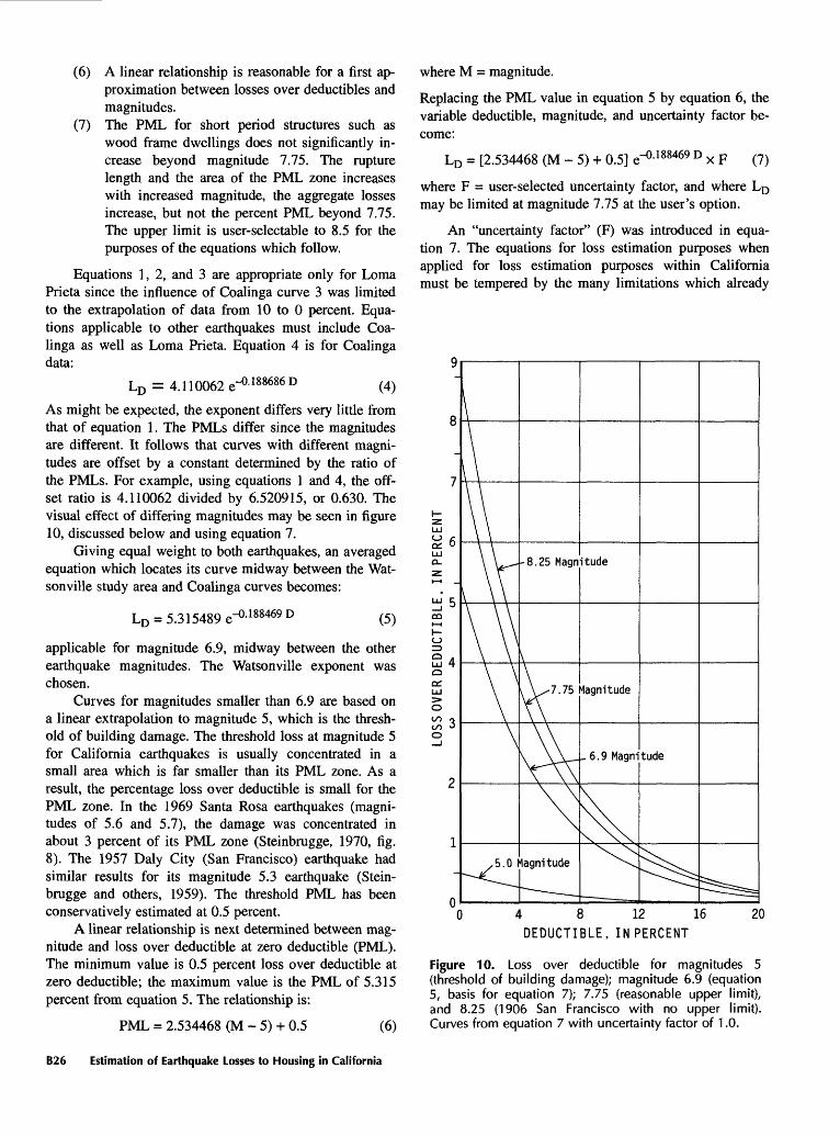
(6) A linear relationship is reasonable for a first ap­ proximation between losses over deductibles and magnitudes.

(7) The PML for short period structures such as wood frame dwellings does not significantly in­ crease beyond magnitude 7.75. The rupture length and the area of the PML zone increases with increased magnitude, the aggregate losses increase, but not the percent PML beyond 7.75. The upper limit is user-selectable to 8.5 for the purposes of the equations which follow.

Equations 1, 2, and 3 are appropriate only for Loma Prieta since the influence of Coalinga curve 3 was limited to the extrapolation of data from 10 to 0 percent. Equa­ tions applicable to other earthquakes must include Coa­ linga as well as Loma Prieta. Equation 4 is for Coalinga data:

LD = 4.110062 e-°- 188686 D (4)

As might be expected, the exponent differs very little from that of equation 1. The PMLs differ since the magnitudes are different. It follows that curves with different magni­ tudes are offset by a constant determined by the ratio of the PMLs. For example, using equations 1 and 4, the off­ set ratio is 4.110062 divided by 6.520915, or 0.630. The visual effect of differing magnitudes may be seen in figure 10, discussed below and using equation 7.

Giving equal weight to both earthquakes, an averaged equation which locates its curve midway between the Wat- sonville study area and Coalinga curves becomes:

LD = 5.315489 e-°- 188469D (5)

applicable for magnitude 6.9, midway between the other earthquake magnitudes. The Watsonville exponent was chosen.

Curves for magnitudes smaller than 6.9 are based on a linear extrapolation to magnitude 5, which is the thresh­ old of building damage. The threshold loss at magnitude 5 for California earthquakes is usually concentrated in a small area which is far smaller than its PML zone. As a result, the percentage loss over deductible is small for the PML zone. In the 1969 Santa Rosa earthquakes (magni­ tudes of 5.6 and 5.7), the damage was concentrated in about 3 percent of its PML zone (Steinbrugge, 1970, fig. 8). The 1957 Daly City (San Francisco) earthquake had similar results for its magnitude 5.3 earthquake (Stein­ brugge and others, 1959). The threshold PML has been conservatively estimated at 0.5 percent.

A linear relationship is next determined between mag­ nitude and loss over deductible at zero deductible (PML). The minimum value is 0.5 percent loss over deductible at zero deductible; the maximum value is the PML of 5.315 percent from equation 5. The relationship is:

where M = magnitude.

Replacing the PML value in equation 5 by equation 6, the variable deductible, magnitude, and uncertainty factor be­ come:

LD = [2.534468 (M - 5) + 0.5] e~°- 188469 D x F (7)

where F = user-selected uncertainty factor, and where LD may be limited at magnitude 7.75 at the user's option.

An "uncertainty factor" (F) was introduced in equa­ tion 7. The equations for loss estimation purposes when applied for loss estimation purposes within California must be tempered by the many limitations which already

PML = 2.534468 (M - 5) + 0.5 (6)

4 8 12 16

DEDUCTIBLE, IN PERCENT

Figure 10. Loss over deductible for magnitudes 5 (threshold of building damage); magnitude 6.9 (equation 5, basis for equation 7); 7.75 (reasonable upper limit), and 8.25 (1906 San Francisco with no upper limit). Curves from equation 7 with uncertainty factor of 1.0.

B26 Estimation of Earthquake Losses to Housing in California

Table 15. Percentage loss over deductible as a function of percent deductible for varying earthquake magnitudes.

[Uncertainty factor = 1. Applicable for post-1939 wood frame dwelling in California. Based on equation 7.]

Percent Deductible

01234567891011121314151617181920

Magnitude5.00

0.500.410.340.280.240.190.160.130.110.090.080.060.050.040.040.030.020.020.020.010.01

5.25

1.130.940.780.640.530.440.370.300.250.210.170.140.120.100.080.070.060.050.040.030.03

5.50

1.771.461.211.000.830.690.570.470.390.320.270.220.180.150.130.100.090.070.060.050.04

5.75

2.401.991.651.361.130.930.770.640.530.440.360.300.250.210.170.140.120.100.080.070.06

6.00

3.032.512.081.721.431.180.980.810.670.560.460.380.320.260.220.180.150.120.100.080.07

6.25

3.673.042.522.081.731.431.180.980.810.670.560.460.380.320.260.220.180.150.120.100.08

6.50

4.303.562.952.442.021.681.391.150.950.790.650.540.450.370.310.250.210.170.140.120.10

6.75

4.944.093.392.802.321.921.591.321.090.910.750.620.510.430.350.290.240.200.170.140.11

7.00

5.574.613.823.162.622.171.801.491.231.020.850.700.580.480.400.330.270.230.190.160.13

7.25

6.205.144.253.522.922.422.001.661.371.140.940.780.650.540.440.370.300.250.210.170.14

7.50

6.845.664.693.883.222.662.211.831.511.251.040.860.710.590.490.400.340.280.230.190.16

7.75

7.476.195.124.243.512.912.412.001.651.371.130.940.780.640.530.440.370.300.250.210.17

8.00

8.106.715.564.603.813.162.622.171.791.491.231.020.840.700.580.480.400.330.270.230.19

8.25

8.747.245.994.964.113.402.822.341.931.601.331.100.910.750.620.520.430.350.290.240.20

have been discussed. This factor may be viewed as being similar to the factor of safety found in building and air­ plane design, in fused electric systems, and the like. It dif­ fers in that this uncertainty factor involves only economic loss and does not involve life loss and injury. As a conse­ quence, users have a wide latitude in the selection of an uncertainty factor. They are urged to examine the model and the data and to select an uncertainty factor to suit their need and their comfort level.

Figure 10 is a graphical representation of equation 7 with an uncertainty factor (F) equal to 1. Curves are shown for: magnitude 5, threshold of damage; magnitude 6.9, average of Watsonville study area and Coalinga; mag­ nitude 7.75, optional limit based on rupture length; and magnitude 8.25, the 1906 San Francisco earthquake. Table 15 is a tabular representation of equation 7.

Equation 7 is simpler and quite different from its post-1939 counterpart found in Steinbrugge and Algermis- sen (1990, p. 60) because of the new Loma Prieta data. The previous PML for magnitude 8.25 with an uncertainty factor of 1 was 4.33 percent; here equation 7 increased the PML to 8.72 percent. Using magnitude 7.75 as the upper limit instead of 8.25, then the 8.72 percent PML would be reduced to 7.46 percent.

The precision of the equations exceed their accuracy. We judge the computational results to be reasonable to one and one-half significant figures, at best. The best reli­ ability is between 5 and 15 percent deductibles and be­ tween magnitudes 6 and 7.5. It remains to be seen how future earthquakes will affect the equations.

1992 Landers Earthquake: California Residential Earthquake Recovery Plan Deductible

Subsequent to the Loma Prieta event, the Landers earthquake of June 28, 1992, provided a partial opportunity to examine equation 7 at low deductibles. Loss information came from the California Residential Earthquake Recovery [Insurance] Plan (CRER). This insurance program, enacted by the California legislature, was in existence for a short period of time before being repealed. Seventeen California earthquakes occurred during the operation of this plan, all in 1992. The Landers earthquake was the only one which contributed a useful amount of data.

Both the CRER deductible and maximum amount of the policy were low, thereby allowing first loss insurance coverage not available in the commercial market. The de­ ductible was one-half of one percent of the amount of the homeowners fire insurance policy, but not less that $1,000. The maximum amount of CRER earthquake insurance was $15,000. A total of 4,341 post-1939 wood frame dwellings had losses over their deductible and with damage not ex­ ceeding the $15,000 policy limit. The dollar deductible when converted to a percentage ranged from 0.5 to 3 per­ cent for almost all of these dwellings.

The number of insured dwellings having losses or losses under the deductible was not available. This meant that equation 7 could not be confirmed by Landers data at low deductibles, but the slope of both curves could be ex­ amined by normalization. Figure 11 shows the equation 7 curve and also the Landers data, normalized at one per­ cent. Slope differences are substantial see the upper right

Dwelling and Mobile Home Monetary Losses Due to the 1989 Loma Prieta, California, Earthquake, with an Emphasis on Loss Estimation B27

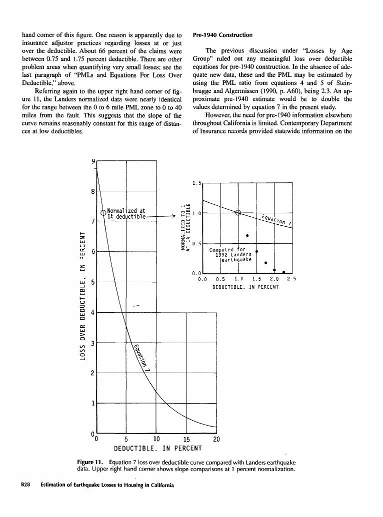
hand corner of this figure. One reason is apparently due to insurance adjuster practices regarding losses at or just over the deductible. About 66 percent of the claims were between 0.75 and 1.75 percent deductible. There are other problem areas when quantifying very small losses; see the last paragraph of "PMLs and Equations For Loss Over Deductible," above.

Referring again to the upper right hand corner of fig­ ure 11, the Landers normalized data were nearly identical for the range between the 0 to 6 mile PML zone to 0 to 40 miles from the fault. This suggests that the slope of the curve remains reasonably constant for this range of distan­ ces at low deductibles.

Pre-1940 Construction

The previous discussion under "Losses by Age Group" ruled out any meaningful loss over deductible equations for pre-1940 construction. In the absence of ade­ quate new data, these and the PML may be estimated by using the PML ratio from equations 4 and 5 of Stein- brugge and Algermissen (1990, p. A60), being 2.3. An ap­ proximate pre-1940 estimate would be to double the values determined by equation 7 in the present study.

However, the need for pre-1940 information elsewhere throughout California is limited. Contemporary Department of Insurance records provided statewide information on the

LLJ 5COh I

oUJo

UJ> ooo oo o

1.5

Normalized at 1* deductible

Computed for 1992 Landers

earthquake

0.5 1.0 1.5 2.0

DEDUCTIBLE, IN PERCENT

2.5

5 10 15 DEDUCTIBLE, IN PERCENT

20

Figure 11 . Equation 7 loss over deductible curve compared with Landers earthquake data. Upper right hand corner shows slope comparisons at 1 percent normalization.

B28 Estimation of Earthquake Losses to Housing in California

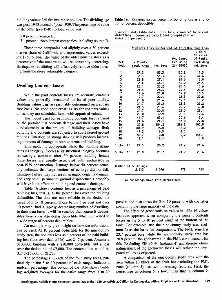
building value of all fire insurance policies. The dividing age was post-1940 instead of post-1939. The percentage of value of the older (pre-1940) to total value was:

5.8 percent, source B,7.1 percent, three largest companies, including source B.

These three companies had slightly over a 50 percent market share of California and represented values exceed­ ing $250 billion. The value of the older housing stock as a percentage of the total value will be constantly decreasing. Earthquake retrofitting will effectively remove older hous­ ing from the more vulnerable category.

Dwelling Contents Losses

While the paid contents losses are accurate, contents values are generally considered to be of poor quality. Building values can be reasonably determined on a square foot basis. No good counterpart exists for contents values unless they are scheduled items with appraised values.

The model used for estimating contents loss is based on the premise that contents damage and their losses have a relationship to the amount of building damage. Both building and contents are subjected to short period ground motions. Duration of strong shaking will produce increas­ ing amounts of damage to both contents and building.

This model is appropriate while the building main­ tains its integrity. Decrease in structural integrity becomes increasingly common after 50 percent building losses; these losses are usually associated with geohazards in post-1939 construction. Damage below 50 percent gener­ ally indicates that large sections of ceilings did not fall. Chimney failure may not result in major contents damage, and very small permanent ground displacements probably will have little effect on building and contents damage.

Table 16 shows contents loss as a percentage of paid building loss, that is, as the percent loss over the building deductible. The data are most reliable in the deductible range of 5 to 10 percent. Those below 5 percent and over 10 percent had a rapidly decreasing number of dwellings in their data base. It will be recalled that source B deduct- ibles were a variable dollar deductible which converted to a wide range of percent deductibles.

An example may give insight on how the information can be used. At 10 percent deductible for the nine-county study area, the contents loss as a percent of the paid build­ ing loss (loss over deductible) was 24.7 percent. Assume a $100,000 building with a $10,000 deductible and a loss over the deductible of $7,000. The contents loss would be 0.247x$7,000, or $1,729.

The percentages in each of the four study areas, par­ ticularly in the 5 to 10 percent of each range, indicate a uniform percentage. The bottom of the table shows build­ ing weighted averages for the entire range from 1 to 20

Table 16. Contents loss as percent of building loss as a func­ tion of percent deductible.

[Source B deductible data, in dollars, converted to percent deductible. Converted deductibles grouped plus or minus 0.5 percent.]

Contents Loss as Percent of Paid Building Loss

Pet. 9-County Ded. Study Area

1234567891011121314151617181920

1 thru 20

5 thru 10

27.333.322.833.425.121.417.619.720.824.721.524.720.042.724.629.8

lOt. 947.285.712.1

22.5

20.8

PML Zone

83.351.327.144.133.226.321.822.421.425.225.630.519.965.424.1

284.216.06.50.0

12.1

26.2

23.7

PML Zone, Excluding ZIP 95030

130.224.224.635.025.024.419.923.519.123.325.725.020.350.633.0

284.216.06.50.0i

23.7

21.9

Within 10 Miles Of Fault, Excluding PML Zone

11.544.618.023.515.621.216.529.618.222.232.823.119.43.429.8100.9

0.0i

143.10.0

21.6

20.6

Number of buildings:2,612 1,096 772 463

buildings have this deductible.

percent and also those for 5 to 10 percent, with the latter containing the large majority of the data.

The effect of geohazards on values in table 16 values becomes apparent when comparing the percent contents losses in the 5 to 10 percent range at the bottom of the table. For example, use the nine-county study area (col­ umn 2) as the basis for comparisons. The PML zone has 23.7 percent loss while the nine-county study area has 20.8 percent; the geohazards in the PML zone account for this. Excluding ZIP 95030 (column 4) and thereby elimi­ nating much of the geohazard losses will reduce the com­ pared values as expected.

A comparison of the nine-county study area with the area within 10 miles of the fault but excluding the PML zone (column 5) has two interesting features. First, the percentage in column 5 is lower than that in column 2.

Dwelling and Mobile Home Monetary Losses Due to the 1989 Loma Prieta, California, Earthquake, with an Emphasis on Loss Estimation B29

Table 17. Contents loss as a percent of building value for nine-county study area.

[Data source B. Limited to buildings having loss over deductible.]

Contents Loss Building As a Percent of Value Building Value

Under $100,000$100,000 - 150,000$150,000 - 200,000$200,000 - 250,000$250,000 - 300,000Over $300,000

3.232.352.703.323.672.95

Number Of

Buildings

265996646341160206

Column 2 percentages contain all geohazards, including those in the San Francisco Marina as well as those in the PML zone; therefore column 2 values should be higher than column 5 values. Of importance is the little differ­ ence in percentages, indicating that the spectacular geo- hazard building damage had little regional impact in the case of the Loma Prieta earthquake. Second and commin­ gled with the first, it also suggests that loss attenuation with distance is not overly important and consistent with our model. The model assumes that magnitude increased the duration of shaking and the accelerations, but did not change the contents to building relationship.

Contents losses will be 20 to 25 percent of structure loss on the average. Many times there will be no structure loss, but contents losses. Similarly, it is possible to have heavy structure loss with minor contents losses. If the de­ ductible is zero, there will be reported contents losses, but equation 8 will overestimate the contents losses, because there is usually no deductible applied to contents losses. Therefore, the amount of contents losses is independent of structure losses by deductible, in the aggregate. The 25 percent reported ratio was based on the reported losses for structure and contents.

Modifying equation 7 to include a user-selectable contents loss factor:

LD = [2.534468 (M - 5) + 0.5] e-°- 188469 D x F X C

where the new term is:

C = factor for contents loss,

which if included as 1.25, the equation then becomes:

LD = [3.168085 (M - 5) + 0.625] e-°- 188469 D x F (8)

and previously defined terms are:

LD = percent loss over deductible,

D = deductible in percent,

Table 18. Ale loss as percent of building loss as a function of percent deductible.

[Source B deductible data, in dollars, converted to percent deductible. Converted deductibles grouped plus or minus 0.5 percent.]

Ale Loss

Pet. 9-County Ded. Study Area

1234567891011121314151617181920

1 thru 20

5 thru 10

0.94.45.111.06.16.87.47.99.110.99.114.214.510.119.08.28.3

30.90.0

19.1

8.4

8.1

as Percent of Paid Building Loss

PML Zone

8.08.25.613.87.59.410.09.99.915.815.116.523.313.322.30.018.80.00.0

19.1

10.8

10.1

PML Zone, Excluding ZIP 95030

11.45.03.112.43.96.44.89.86.412.210.914.614.010.711.50.018.80.00.0i

8.0

7.3

Within 10 mil es Of Fault, Excluding PML Zone

0.00.00.03.64.98.14.39.77.93.30.410.00.18.114.758.90.0i

0.01

6.0

7.0

Number of buildings:2,612 1,096 772 463

*No buildings have this deductible.

M = magnitude, and

F = user-selected uncertainty factor.

When settling earthquake claims, source B had a prac­ tice whereby contents and Ale losses were paid in full up to the earthquake insured limit and applied the deductible to the structure loss if the contents and Ale loss did not ex­ haust the limit. Not all companies followed this procedure. Comparisons showed that this variability was minor except where numerous large geohazard losses occurred.

Table 17 shows the variations of contents loss as a percent of building value. The lowest and highest value groupings are contrary to the ascending order of percent­ ages in the second column.

B30 Estimation of Earthquake Losses to Housing in California

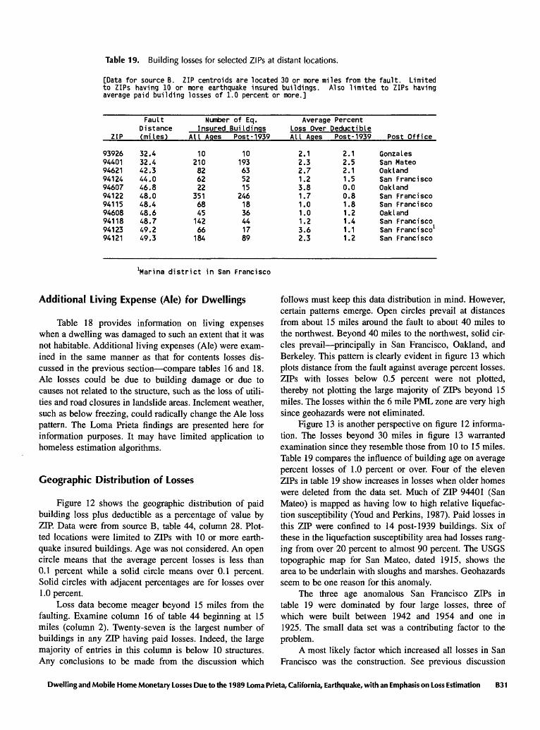
Table 19. Building losses for selected ZIPs at distant locations.

[Data for source B. ZIP centroids are located 30 or more miles from the fault. Limited to ZIPs haying 10 or more earthquake insured buildings. Also limited to ZIPs having average paid building losses of 1.0 percent or more.]

ZIP

9392694401946219412494607941229411594608941189412394121

Fault Distance (miles)

32.432.442.344.046.848.048.448.648.749.249.3

Number Insured

All Ages

10210826222

351684514266184

of Eq. Bui I dingsPost -1939

10193635215

2461836441789

Average Loss Over All Ages

2.12.32.71.23.81.71.01.01.23.62.3

Percent Deductible Post -1939

2.12.52.11.50.00.81.81.21.41.11.2

Post Office

GonzalesSan MateoOaklandSan FranciscoOaklandSan FranciscoSan FranciscoOaklandSan FranciscoSan Francisco1San Francisco

Marina district in San Francisco

Additional Living Expense (Ale) for Dwellings

Table 18 provides information on living expenses when a dwelling was damaged to such an extent that it was not habitable. Additional living expenses (Ale) were exam­ ined in the same manner as that for contents losses dis­ cussed in the previous section compare tables 16 and 18. Ale losses could be due to building damage or due to causes not related to the structure, such as the loss of utili­ ties and road closures in landslide areas. Inclement weather, such as below freezing, could radically change the Ale loss pattern. The Loma Prieta findings are presented here for information purposes. It may have limited application to homeless estimation algorithms.

Geographic Distribution of Losses

Figure 12 shows the geographic distribution of paid building loss plus deductible as a percentage of value by ZIP. Data were from source B, table 44, column 28. Plot­ ted locations were limited to ZIPs with 10 or more earth­ quake insured buildings. Age was not considered. An open circle means that the average percent losses is less than 0.1 percent while a solid circle means over 0.1 percent. Solid circles with adjacent percentages are for losses over 1.0 percent.

Loss data become meager beyond 15 miles from the faulting. Examine column 16 of table 44 beginning at 15 miles (column 2). Twenty-seven is the largest number of buildings in any ZIP having paid losses. Indeed, the large majority of entries in this column is below 10 structures. Any conclusions to be made from the discussion which

follows must keep this data distribution in mind. However, certain patterns emerge. Open circles prevail at distances from about 15 miles around the fault to about 40 miles to the northwest. Beyond 40 miles to the northwest, solid cir­ cles prevail principally in San Francisco, Oakland, and Berkeley. This pattern is clearly evident in figure 13 which plots distance from the fault against average percent losses. ZIPs with losses below 0.5 percent were not plotted, thereby not plotting the large majority of ZIPs beyond 15 miles. The losses within the 6 mile PML zone are very high since geohazards were not eliminated.

Figure 13 is another perspective on figure 12 informa­ tion. The losses beyond 30 miles in figure 13 warranted examination since they resemble those from 10 to 15 miles. Table 19 compares the influence of building age on average percent losses of 1.0 percent or over. Four of the eleven ZIPs in table 19 show increases in losses when older homes were deleted from the data set. Much of ZIP 94401 (San Mateo) is mapped as having low to high relative liquefac­ tion susceptibility (Youd and Perkins, 1987). Paid losses in this ZIP were confined to 14 post-1939 buildings. Six of these in the liquefaction susceptibility area had losses rang­ ing from over 20 percent to almost 90 percent. The USGS topographic map for San Mateo, dated 1915, shows the area to be underlain with sloughs and marshes. Geohazards seem to be one reason for this anomaly.

The three age anomalous San Francisco ZIPs in table 19 were dominated by four large losses, three of which were built between 1942 and 1954 and one in 1925. The small data set was a contributing factor to the problem.

A most likely factor which increased all losses in San Francisco was the construction. See previous discussion

Dwelling and Mobile Home Monetary Losses Due to the 1989 Loma Prieta, California, Earthquake, with an Emphasis on Loss Estimation B31

MONTEREY

BAY

B32 Estimation of Earthquake Losses to Housing in California

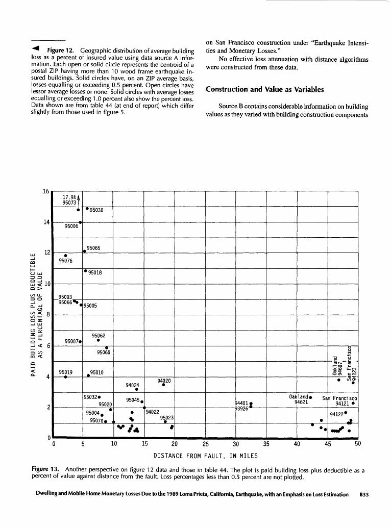
"^ Figure 12. Geographic distribution of average building loss as a percent of insured value using data source A infor­ mation. Each open or solid circle represents the centroid of a postal ZIP having more than 10 wood frame earthquake in­ sured buildings. Solid circles have, on an ZIP average basis, losses equalling or exceeding 0.5 percent. Open circles have lessor average losses or none. Solid circles with average losses equalling or exceeding 1.0 percent also show the percent loss. Data shown are from table 44 (at end of report) which differ slightly from those used in figure 5.

on San Francisco construction under "Earthquake Intensi­ ties and Monetary Losses."

No effective loss attenuation with distance algorithms were constructed from these data.

Construction and Value as Variables

Source B contains considerable information on building values as they varied with building construction components

16

14

12

17.9JU 95073

*

95006

95076

9500395066 *.

95007*

95019

95030

m 95065

95018

95005

95062

95060

^95010

95032* 95020

95004 0 * 95070*

94024

95045.

%

v /*

94020

9402295023 t

34401* 33926-*

Oakland* sa 94621

8 v>1 1 .ID h~ ID

** <£> U. COID ** e\jOCTl CrH

oooi

i Francisco 94121

94122*~f

O LlJ _j _j

Q _l LU <

00 <

10

< 6=3 «/> £0 <

Q

<

10 15 20 25 30 35

DISTANCE FROM FAULT, IN MILES

40 45 50

Figure 13. Another perspective on figure 12 data and those in table 44. The plot is paid building loss plus deductible as a percent of value against distance from the fault. Loss percentages less than 0.5 percent are not plotted.

Dwelling and Mobile Home Monetary Losses Due to the 1989 Loma Prieta, California, Earthquake, with an Emphasis on Loss Estimation B33

Table 20. Number of stories as a function of building losses.

Table 21. Type of roof as a func­ tion of building losses.

[Data from source B. ZIPs within 10 miles of the fault. Wood frame, post-1939 construction. Losses are before the deductible.]

[Data from source B. ZIPs within 10 miles of the fault. Wood frame, post-1939 construction. Losses are before the deductible.]

Number Number of Stories Buildings

123

Bi level1 & half2 & half3 levelUnknown

428258

39

1211

25538

Bldg. Loss As Pet.

Of Value

18.517.311.115.019.08.016.220.0

such as type of roof and number of stories. Numerous combi­ nations were examined, with the more interesting of these summarized below.

Tables 20, 21, 22, and 23 are limited to post-1939 dwellings within 10 miles of the surface projection of the fault. An important factor in all tables, except table 23, is that the column "Building Loss as a Percent of Value" is based only on dwellings having paid losses, excluding dwellings which did not have losses over the deductible. Therefore, the percentages are not PML values and are only useful as relative values.

Table 20 shows the percent building loss as a function of the number of stories. The table clearly demonstrates that two story structures performed as well as one story structures. This observation does not apply to dwellings in San Francisco; see discussion under "Monetary Loss," above.

Tile roofs are often considered to be both a life haz­ ard and to be vulnerable to damage. Table 21 may be sur­ prising with respect to dollar loss. Type of tile anchorage to its supporting members, if any, is unknown. Dollar loss is not necessarily indicative of life hazard, such as tile over exit doorways.

Masonry chimneys are especially vulnerable to dam­ age when they are unreinforced. Fewer fail when they are reinforced, and essentially none fail when the shaking is not severe. Table 22 shows data for losses over the deduct­ ible in the heavily shaken area. There was no breakdown on reinforced and nonreinforced chimneys. The loss per­ centages in the last column indicate that building losses over the deductible, if anything, tend to decrease with an increase in the number of chimneys.

Table 23 relates dwelling value to the percentage of owners who chose earthquake insurance in addition to their fire coverage. The percentages increase from the

RoofType

Tile1OtherUnknown

Number ofBui I dings

61538784

Bldg. LossAs Pet.

Of Value

17.320.018.0

or concrete

Table 22. Masonry chimneys as a function of building losses.

[Data from source B. ZIPs within 10 miles of the fault. Wood frame, post-1939 construction. Losses are before the deductible.]

Number Masonry Chimneys

None1234

Number of Bui I dings

178513129214

Bldg. Loss As Pet.

Of Value

20.117.915.415.730.2

Table 23. Value as a function of earthquake insurance coverage.

[Data from source B. ZIPs within 10 miles of the fault. Wood frame, post- 1939 construction. Losses are before the deductible.]

Building Value

x$1000

Less $100$101-150$151-200$201-250$251-300$301-350$351-400$401-450$451-500$501-550$551-600$601-650$651-700$701-750Over $750

Number of Bui I dings

6,80413,2377,1072,8121,19352222710663474524101236

Pet. With Eq. Insurance

19.536.448.554.658.861.556.853.857.159.668.975.070.075.055.6

B34 Estimation of Earthquake Losses to Housing in California

under $100,000 dwellings to about $300,000, then tend to erratically increase. This indicates that the homeowner's economic status is an important factor in the purchase of earthquake insurance.

Modified Mercalli Intensity

Shown in figure 14 are the boundaries of the 6-mile PML zone and a portion of the Modified Mercalli intensity map including the epicentral area. The isoseismal line is from a portion of figure 2 in Stover and others (1990). The correlation between the theoretic PML zone and the iso­ seismal map is reasonable in the populated areas. The ab­ sence of dwellings and other structures in much of the Santa Cruz Mountains leaves the northeastern boundaries mostly undocumented (see fig. 3).

One comparison between intensity VHI and quantified dwelling losses for post-1939 construction is:

Percent PML

1989 Loma Prieta (equations 1, 2, and 3)

PML zone, including geohazards

PML zone, excluding geohazards

Watsonville study area

1983 Coalinga

17.5

12.4

6.5

4.6

Correlations between mapped intensity and actual losses are not simple.

Other comparisons from other earthquakes show wide variations among intensities and losses (table 28 in Stein- brugge and Algermissen, 1990) and should be examined in the context of the above tabulation.

The definitions and interpretations of Modified Mer­ calli intensities commingled incompatible factors such as (1) human response, (2) functional impairments, (3) de­ gree of building damage, and (4) geologic effects. The definitions use nonqualified as well as subjective termi­ nology: "few," "many," "slight," "considerable," "good," and "frightened all." These terms are summarized by an intensity. A single intensity may be assigned to a specific site or more often to a large area (Steinbrugge, 1986).

There is a role for specialized equivalents to intensity maps intended for specific purposes such as monetary loss and life safety estimates. Such maps require data bases of structures by construction class, occupancy types, and oc­ cupant loads. These data bases must include values and losses sustained as well as a measure of local dynamic soil conditions. These data are often found in geographically scattered computerized systems compiled by governmen­ tal, academic, and private entities.

While one of the authors (Steinbrugge) has used Modified Mercalli intensities in previous studies, alterna­ tives have also been examined. One alternative is con­ tained in this paper. On the other hand and much in the maps' favor, they provide an excellent overview of overall effects and are vital to the historic record.

MOBILE HOMES (MANUFACTURED HOUSING)

Introduction

Information on mobile home damage and losses from the Loma Prieta earthquake came from three sources: source B (previously discussed), source C (new), and the California Department of Housing and Community Development (new). Additionally, a retrospective study of previous Cali­ fornia mobile home experience is included for the following earthquakes: 1971 San Fernando, 1978 Santa Barbara, 1979 El Centre (Imperial Valley), 1980 Livermore (Greenville), and 1983 Coalinga. Other earthquakes provided little useful information for monetary loss estimation. Although data for the 1984 Morgan Hill earthquake are only minimally useful, 17 mobile homes representing 2 percent of the mobile home units in the Morgan Hill and Gilroy areas fell. No damage was found to coaches having a proprietary earthquake brac­ ing system although nearby unbraced ones fell (Kensler, 1985). Monetary losses were not estimated.

The number of spaces available for mobile homes is listed in some data bases. Since mobile home parks are normally at capacity, or very close thereto, the number of coaches in a park is considered to be the same as the num­ ber of spaces. Mobile homes, coaches, and manufactured housing have the same meanings in this study. They may or may not include contents and appurtenances, depending upon context.

Definition Of Mobile Home (Manufactured Housing)

A mobile home (manufactured housing) is defined here to mean a coach unit which is transported (towed) on wheels to a site where it can be jacked or raised off its wheels and leveled. The wheels, but not the axle spindles and drum unit to which the wheels and tires fasten, may be removed and stored.

The typical set-up technique for a mobile home is to roll the coach into place and use one of several types of piers placed at intervals of about 6 feet along the main frame. A screwjack on the top of each metal pier is then brought up into contact with the undercarriage and posi­ tioned until the coach is level and steady on the mounts.

Dwelling and Mobile Home Monetary Losses Due to the 1989 Loma Prieta, California, Earthquake, with an Emphasis on Loss Estimation B35

Boundary o

f ZI

Ps w

ith

centroids

in t

he P

ML z

one

Figu

re 1

4.

PM

L zo

ne a

nd i

ts r

elat

ions

hips

to

the

Mod

ified

Mer

calli

in

tens

ity z

one

VIII

. A

lso

show

n is

the

boun

dary

of

the

ZIPs

with

cen

troi

ds w

ithin

the

PM

L zo

ne.

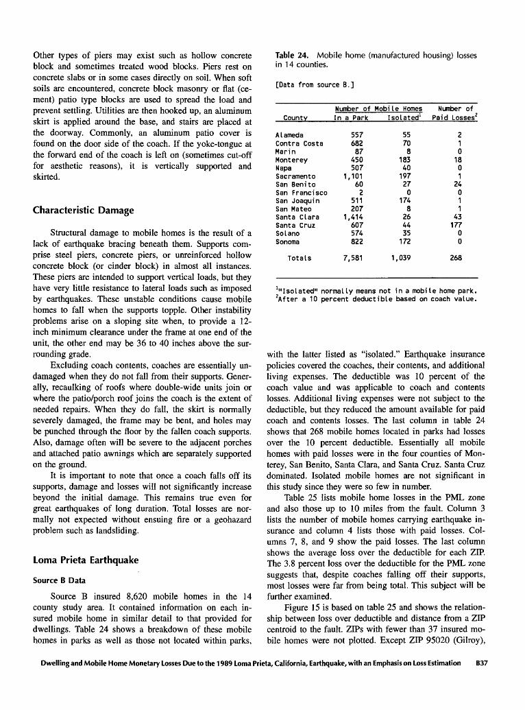
Other types of piers may exist such as hollow concrete block and sometimes treated wood blocks. Piers rest on concrete slabs or in some cases directly on soil. When soft soils are encountered, concrete block masonry or flat (ce­ ment) patio type blocks are used to spread the load and prevent settling. Utilities are then hooked up, an aluminum skirt is applied around the base, and stairs are placed at the doorway. Commonly, an aluminum patio cover is found on the door side of the coach. If the yoke-tongue at the forward end of the coach is left on (sometimes cut-off for aesthetic reasons), it is vertically supported and skirted.

Characteristic Damage

Structural damage to mobile homes is the result of a lack of earthquake bracing beneath them. Supports com­ prise steel piers, concrete piers, or unreinforced hollow concrete block (or cinder block) in almost all instances. These piers are intended to support vertical loads, but they have very little resistance to lateral loads such as imposed by earthquakes. These unstable conditions cause mobile homes to fall when the supports topple. Other instability problems arise on a sloping site when, to provide a 12- inch minimum clearance under the frame at one end of the unit, the other end may be 36 to 40 inches above the sur­ rounding grade.

Excluding coach contents, coaches are essentially un­ damaged when they do not fall from their supports. Gener­ ally, recaulking of roofs where double-wide units join or where the patio/porch roof joins the coach is the extent of needed repairs. When they do fall, the skirt is normally severely damaged, the frame may be bent, and holes may be punched through the floor by the fallen coach supports. Also, damage often will be severe to the adjacent porches and attached patio awnings which are separately supported on the ground.

It is important to note that once a coach falls off its supports, damage and losses will not significantly increase beyond the initial damage. This remains true even for great earthquakes of long duration. Total losses are nor­ mally not expected without ensuing fire or a geohazard problem such as landsliding.

Loma Prieta Earthquake

Source B Data

Source B insured 8,620 mobile homes in the 14 county study area. It contained information on each in­ sured mobile home in similar detail to that provided for dwellings. Table 24 shows a breakdown of these mobile homes in parks as well as those not located within parks,

Table 24. Mobile home (manufactured housing) losses in 14 counties.

[Data from source B.]

Number of Mobile HomesCounty

A I amedaContra CostaMar inMontereyNapaSacramentoSan Bern" toSan FranciscoSan JoaquinSan MateoSanta ClaraSanta CruzSolanoSonoma

In a Park

55768287

450507

1,101602

511207

1,414607574822

Isolated1

55708

18340197270

1748264435172

Number of Paid Losses2

210

1801

24011

43177

00

Totals 7,581 1,039 268

lM Isolated" normally means not in a mobile home park. 2After a 10 percent deductible based on coach value.

with the latter listed as "isolated." Earthquake insurance policies covered the coaches, their contents, and additional living expenses. The deductible was 10 percent of the coach value and was applicable to coach and contents losses. Additional living expenses were not subject to the deductible, but they reduced the amount available for paid coach and contents losses. The last column in table 24 shows that 268 mobile homes located in parks had losses over the 10 percent deductible. Essentially all mobile homes with paid losses were in the four counties of Mon­ terey, San Benito, Santa Clara, and Santa Cruz. Santa Cruz dominated. Isolated mobile homes are not significant in this study since they were so few in number.

Table 25 lists mobile home losses in the PML zone and also those up to 10 miles from the fault. Column 3 lists the number of mobile homes carrying earthquake in­ surance and column 4 lists those with paid losses. Col­ umns 7, 8, and 9 show the paid losses. The last column shows the average loss over the deductible for each ZIP. The 3.8 percent loss over the deductible for the PML zone suggests that, despite coaches falling off their supports, most losses were far from being total. This subject will be further examined.

Figure 15 is based on table 25 and shows the relation­ ship between loss over deductible and distance from a ZIP centroid to the fault. ZIPs with fewer than 37 insured mo­ bile homes were not plotted. Except ZIP 95020 (Gilroy),

Dwelling and Mobile Home Monetary Losses Due to the 1989 Loma Prieta, California, Earthquake, with an Emphasis on Loss Estimation B37

Table 25. Mobile home losses 10 miles or less from the fault.

[Data from source B. excluding ZIP 95030. Deductible is 10 percent of coach value and applies to coach plus contents losses. ZIP to fault distances are to the ZIP centroid and not to centroid of parks. Only ZIPs with earthquake insurance are included.]

Number of Mobile Koines

ZIP to Fault WithDistance Eq.

ZIP (miles) Insur.

WithPaidLoss

Value x$1000Coach Conts.

Paid Loss x$1000Coach Conts. Ale

PercentCoach

Loss OverDeductible

PML zone

9507695003950669507395006950059506595018

Totals

9506295060950209390795124

Totals

2.13.53.94.34.74.85.35.5

PML zone

7.58.99.610.010.0

, all of

1596379823406

396

Beyond PML

1683837140

1

above 780

691417260202

130

zone but

324

1160

183

7,0243,1365,1213,421

61900

143

18,996

within

5,5531,9621,4224,482

37

32,452

5,7352,5594,4863,019

48680

106

16,021

10 miles

4,5361,6011,1273,722

28

27,035

32869183135

0602

723

of the

517

48340

864

1668562470301

365

fault

302940

410

59812170100

96

40120

103

4.72.23.64.00.06.70.01.2

3.8

0.90.43.40.80.0

2.7

LU_1 00 I II oZD O LU O

I z.LUI O Z. C£LU LUCJO-CE:

LU CSQ.

oiLU> o0000o

1 o < o o

I rv>

90576Watsonville

95003Aptos

95073Soquel

95066Santa Cruz

95062Santa Cruz

9

95020 Gilroy

93707 <Salinas

5060 Santa Cruz

2468

DISTANCE FROM FAULT, IN MILES

10

Figure 15. Loma Prieta earthquake. Mobile home loss over 10 percent deductible as a function of distance from the fault for parks are grouped by ZIP; in figure 16, parks are individ­ ually plotted. Excluded are ZIPs with no losses or fewer than 10 mobile homes. Names are post office names and may include large rural areas. Data from source B.

the data are well-behaved and suggest a curve for the upper limit of distance versus coach losses. This relation­ ship would be limited to the 10 percent deductible.

An alternate viewpoint of loss versus distance is fig­ ure 16 where the distances from individual mobile home parks to the fault are shown. Distances are those from the parks and not from ZIP centroids. The triangles are for the Watsonville ZIP; these parks are also those closest to the fault. Solid circles are those parks along Monterey Bay plus those westerly of the fault. Open circles are for parks east of the fault from the Santa Clara Valley southward to Hollister. Data scatter among parks can be attributed to local soil conditions and also to type of piers supporting the coach (see a following discussion under "California Department of Housing and Community Development"). Directionality of seismic waves and soil amplification of ground motions may have contributed in some instances. Parks with fewer than 10 insured mobile homes were ex­ cluded. Some contiguous parks were combined. The large loss of 5.2 percent at distance 14 miles (San Jose) is due to heavy damage to one coach out of 12.

Information additional to figure 16 losses in Watson­ ville, Corralitos, Gilroy, and Hollister is shown in table 26. The Watsonville and near vicinity mobile home information

B38 Estimation of Earthquake Losses to Housing in California

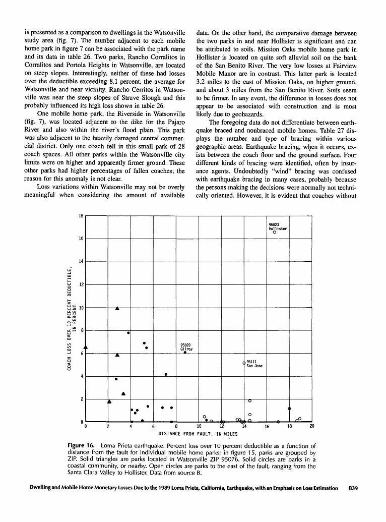
is presented as a comparison to dwellings in the Watsonville study area (fig. 7). The number adjacent to each mobile home park in figure 7 can be associated with the park name and its data in table 26. Two parks, Rancho Corralitos in Corralitos and Portola Heights in Watsonville, are located on steep slopes. Interestingly, neither of these had losses over the deductible exceeding 8.1 percent, the average for Watsonville and near vicinity. Rancho Cerritos in Watson­ ville was near the steep slopes of Struve Slough and this probably influenced its high loss shown in table 26.

One mobile home park, the Riverside in Watsonville (fig. 7), was located adjacent to the dike for the Pajaro River and also within the river's flood plain. This park was also adjacent to the heavily damaged central commer­ cial district. Only one coach fell in this small park of 28 coach spaces. All other parks within the Watsonville city limits were on higher and apparently firmer ground. These other parks had higher percentages of fallen coaches; the reason for this anomaly is not clear.

Loss variations within Watsonville may not be overly meaningful when considering the amount of available

data. On the other hand, the comparative damage between the two parks in and near Hollister is significant and can be attributed to soils. Mission Oaks mobile home park in Hollister is located on quite soft alluvial soil on the bank of the San Benito River. The very low losses at Fairview Mobile Manor are in contrast. This latter park is located 3.2 miles to the east of Mission Oaks, on higher ground, and about 3 miles from the San Benito River. Soils seem to be firmer. In any event, the difference in losses does not appear to be associated with construction and is most likely due to geohazards.

The foregoing data do not differentiate between earth­ quake braced and nonbraced mobile homes. Table 27 dis­ plays the number and type of bracing within various geographic areas. Earthquake bracing, when it occurs, ex­ ists between the coach floor and the ground surface. Four different kinds of bracing were identified, often by insur­ ance agents. Undoubtedly "wind" bracing was confused with earthquake bracing in many cases, probably because the persons making the decisions were normally not techni­ cally oriented. However, it is evident that coaches without

18

16

14

12

10

95033 Hol1ister

O

95020 Gilroy

(1,95111 San Jose

6 8 10 12 14

DISTANCE FROM FAULT. IN MILES

16 18 20

Figure 16. Loma Prieta earthquake. Percent loss over 10 percent deductible as a function of distance from the fault for individual mobile home parks; in figure 15, parks are grouped by ZIP. Solid triangles are parks located in Watsonville ZIP 95076. Solid circles are parks in a coastal community, or nearby. Open circles are parks to the east of the fault, ranging from the Santa Clara Valley to Hollister. Data from source B.

Dwelling and Mobile Home Monetary Losses Due to the 1989 Loma Prieta, California, Earthquake, with an Emphasis on Loss Estimation B39

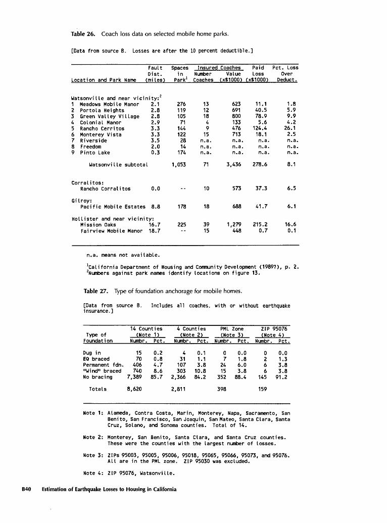
Table 26. Coach loss data on selected mobile home parks.

[Data from source B. Losses are after the 10 percent deductible.]

Fault Spaces Insured Coaches Paid Pet. LossDist. in Number Value Loss Over

Location and Park Name (miles) Park1 Coaches (x$1000) (x$1000) Deduct.

Watsonville and near vicinity:1 Meadows Mobile Manor 2.1 276 13 623 112 Portola Heights 2.8 119 12 691 40.3 Green Valley Village 2.8 105 18 800 78.4 Colonial Manor 2.9 71 4 133 5.5 Rancho Cerritos 3.3 144 9 476 124.6 Monterey Vista 3.3 122 15 713 18.7 Riverside 3.5 28 n.a. n.a. n.a.8 Freedom 2.0 14 n.a. n.a. n.a.9 Pinto Lake 0.3 174 n.a. n.a. n.a.

Watsonville subtotal 1,053 71 3,436 278.6

1.8 5.9 9.9 4.2

26.1 2.5 n.a. n.a. n.a.

8.1

Corralitos:Rancho Corralitos 0.0

Gilroy:Pacific Mobile Estates 8.8 178

Hoi lister and near vicinity:Mission Oaks 16.7 225 Fair-view Mobile Manor 18.7

10

18

3915

573 37.3

688 41.7

6.5

6.1

1,279 215.2 16.6448 0.7 0.1

n.a. means not available.

California Department of Housing and Community Development (1989?), p. 2. 2Numbers against park names identify locations on figure 13.

Table 27. Type of foundation anchorage for mobile homes.

[Data from source B. Includes all coaches, with or without earthquake insurance.]

14 CountiesType ofFoundation

Dug inEQ bracedPermanent fdn."Wind" bracedNo bracing

(NoteNumbr.

1570

406740

7,389

1)4 Counties(Note 2)

Pet.

0.0.4.8.

85.

28767

Numbr.

431107303

2,366

Pet.

0.1.3.

10.84.

11882

PML Zone(Note 3)

Numbr.

07

2415

352

Pet.

0.01.86.03.8

88.4

ZIP 95076(Note

Numbr.

0266

145

4 )Pet.

0133

91

.0

.3

.8

.8

.2

Totals 8,620 2,811 398 159

Note 1: Alameda, Contra Costa, Marin, Monterey, Napa, Sacramento, San Bern"to, San Francisco, San Joaquin, San Mateo, Santa Clara, Santa Cruz, Solano, and Sonoma counties. Total of 14.

Note 2: Monterey, San Benito, Santa Clara, and Santa Cruz counties. These were the counties with the largest number of losses.

Note 3: ZIPs 95003, 95005, 95006, 95018, 95065, 95066, 95073, and 95076. All are in the PML zone. ZIP 95030 was excluded.

Note 4: ZIP 95076, Watsonville.

B40 Estimation of Earthquake Losses to Housing in California

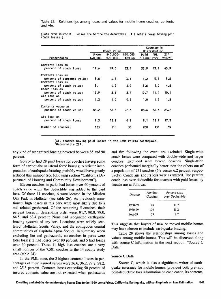
Table 28. Relationships among losses and values for mobile home coaches, contents, and Ale.

[Data from source B. Losses are before the deductible. All mobile homes having paid coach losses.]

Percentages

Coach ValueUnder $40,000- $70,000

$40.000 $70.000 And UD

Geographic Distribution

Paid PML ZIP Claims 1 Zone 950762

Contents loss as percent of coach loss: 19.6 49.0 33.4

Contents loss aspercent of contents value: 3.8 4.8 3.1

Contents loss aspercent of coach value: 3.1 4.2 2.9

Coach loss aspercent of coach value: 15.9 8.6 8.7

Ale loss aspercent of coach value: 1.2 1.0 0.5

Contents value aspercent of coach value: 88.2 86.5 92.6

Ale loss aspercent of coach loss: 7.3 12.2 6.2

Number of coaches: 123 115 30

33.9 43.9 45.9

4.2 5.8 5.6

3.6 5.0 4.6

10.7 11.4 10.1

1.0 1.5 1.8

88.6 86.6 83.2

9.1 12.9 17.3

268 131 69

JAll coaches having paid losses in the Loma Prieta earthquake.Watsonville ZIP.

any kind of recognized bracing hovered between 85 and 90 percent.

Source B had 28 paid losses for coaches having some form of earthquake or lateral force bracing. A stricter inter­ pretation of earthquake bracing probably would have greatly reduced this number (see following section "California De­ partment of Housing and Community Development").

Eleven coaches in parks had losses over 60 percent of coach value when the deductible was added to the paid loss. Of these 11 coaches, 6 were located in the Mission Oak Park in Hollister (see table 26). As previously men­ tioned, high losses in this park were most likely due to a soil related geohazard. Of the remaining 5 coaches, their percent losses in descending order were: 91.7, 90.8, 79.0, 64.5, and 63.4 percent. None had recognized earthquake bracing systems of any sort. Locations were widely scat­ tered: Hollister, Scotts Valley, and the contiguous coastal communities of Capitola-Aptos-Soquel. In summary when excluding fire and geohazards, no coaches in parks were total losses: 2 had losses over 80 percent, and 5 had losses over 60 percent. These 11 high loss coaches are a very small number of the 7,581 coaches in the 14 county study area (table 24).

In the PML zone, the 5 highest contents losses in per­ centages of their insured values were 36.6, 36.2, 29.8, 28.2, and 25.5 percent. Contents losses exceeding 50 percent of insured contents value are not expected when geohazards

and fire following the event are excluded. Single-wide coach losses were compared with double-wide and larger coaches. Excluded were braced coaches. Single-wide coaches performed marginally better than the others out of a population of 231 coaches (5.9 versus 6.2 percent, respec­ tively). Coach age and its loss were examined. The percent coach loss over deductible for coaches with paid losses by decade are as follows:

Decade

1960-69

1970-79

Post-79

Number Percent Loss Coaches over Deductible

49

179

39

11.7

11.2

8.2

This suggests that buyers of new or moved mobile homes may have chosen to include earthquake bracing.

Table 28 shows the relationships among losses and values among mobile homes. This will be discussed along with source C information in the next section, "Source C Data."

Source C Data

Source C, which is also a significant writer of earth­ quake insurance for mobile homes, provided both pre- and post-deductible loss information on each coach, its contents,

Dwelling and Mobile Home Monetary Losses Due to the 1989 Loma Prieta, California, Earthquake, with an Emphasis on Loss Estimation B41

Table 29. Mobile homes with paid losses in the PML zone.

[Data from sources B and C. ZIP 95030 excluded.]

Mobile Homes With Paid Losses

ZIP

9507695003950669507395006950059506595018

Post office

Watsonvi I leAptosSanta CruzSequelBoulder CreekBen LomondSanta CruzFelton

Source B

691417260202

Source C

54173150000

Totals 130 107

and Ale (loss due to additional living expenses). Source C information was by ZIP code and not by address. It lacked information on insured mobile homes not having paid losses. This lack precluded an analysis of loss over deduct­ ible and of PML values.

Source C had 228 paid mobile home claims, 3 with ensuing fire loss. Of these, 179 had a 5 percent deductible; 29 had a 2 percent deductible; and 17 had other deduct- ibles. Of the fire losses, one was a total loss, the second had a 70 percent loss before the deductible, and the third was under 50 percent. There were 107 paid claims within the PML zone, excluding ZIP 95030. By comparison, source B had 268 paid claims over the 10 percent deductible. A more detailed comparison on a ZIP basis for the PML zone is shown in table 29.

Ratios in the form of percentages among coaches, contents, and Ale are given in tables 28 and 30. These

Table 30. Relationships among losses and values for mobile home coaches, contents, and Ale.

[Data from source C and combined sources B and C. Losses are before the deductible. All mobile homes having paid coach losses.]

Coach ValuePercentages Under

$40.000$40,000- $70.000

$70,000 And UD

Geographic Distribution

Paid Claims1

PML Zone

ZIP 950762

SOURCE C

Contents loss as percent of coach loss: 30.1 30.8 52.6

WEIGHTED AVERAGES OF SOURCES B AND C

34.7 34.6 27.4

Contents loss as percent of contents value:Contents loss as percent of coach value:Coach loss as percent of coach value:Ale loss as percent of coach value:

Contents value as percent of coach value:

Ale loss as percent of coach loss:

Number of coaches:

8.64.916.31.2

56.8

7.3

37

8.54.615.00.9

54.3

6.1

151

12.66.812.90.5

53.8

3.7

30

9.45.114.70.9

54.4

5.8

218

12.56.819.71.3

54.6

6.5

104

15.38.1

29.42.3

52.7

7.7

53

Contents loss as percent of coach loss: 22.5 36.1 45.1

Contents loss as percent of contents value: 4.8 6.6 6.7Contents loss as percent of coach value: 3.6 4.4 4.9Coach loss as percent of coach value: 16.0 12.3 10.9Ale loss as percent of coach value: 1.2 1.0 0.5

Contents value as percent of coach value: 75.4 67.7 72.7

Ale loss as percent of coach loss: 7.3 7.9 4.7

Number of coaches: 160 266 60

34.4 38.2 32.7

6.24.4

8.35.9

12.7 15.40.9 1.4

9.06.2

19.12.0

70.2 70.7 69.0

7.2 8.9 10.4

486 235 122

*AU coaches having paid losses in the Loma Prieta earthquake. Stetsonville ZIP.

B42 Estimation of Earthquake Losses to Housing in California

percentages fall into two categories: (1) coach value, and (2) geographic distribution. The percentages give insights into data comparisons and thereby indicate the variations which may be expected among various data sources. Sec­ ondly, they provide a basis for loss estimation applica­ tions. For example, visual inspections may allow quick estimates on the amount of coach damage and thereby coach loss; the contents loss to coach loss percentage al­ lows a quick estimate on the amount of contents loss when visual inspections must be limited to the exteriors. This will be further discussed under "Test of Rapid Loss Esti­ mation, El Centro." Thirdly and for loss estimation for postulated earthquakes, the percentages allow for estimates on other losses when the PML has been determined. Ta­ bles 28 and 30 are pilot in nature and should be used with considerable care and judgment.

A detailed example of one application is examined. Columns 5 and 6 of tables 28 and 30 may be the more significant of those in these tables. Compare contents loss as a percent of coach loss for both sources B and C first line in each table. Source C values (table 30) are essen­ tially identical: 34.7 percent and 34.6 percent; those for source B are 33.9 percent and 43.9 percent. This is better agreement than might be expected. The weighted averages of these are found on the bottom half of table 30: 34.4 percent and 38.2 percent, respectively. For applications, one may reasonably judge an average of 1/3, that is, on an aggregate basis the contents loss will be 1/3 of that for the coach. A similar approach was used for wood frame dwellings where, in table 16, the average was about 1/4 instead of 1/3. The commentary on the dwelling percent­ age also largely applies here and should be referred to for additional information. In the case of mobile homes where coaches can readily fall from their vertical supports, con­ tents losses may be large for items such as overturned re­ frigerators which may not overturn in dwellings remaining on their foundations. This is one seeming explanation for the mobile home percentages averaging around 30 to 35 percent while those for wood frame dwellings were about 20 to 25 percent (table 16). Only experience from future earthquakes will provide definitive percentages for tables 28 and 30.

Not all comparisons are as good. Potential sources of errors inherent in all comparisons are company market shares which differ among parks and their geohazards.

California Department of Housing and Community Development

The California Department of Housing and Commu­ nity Development (acronym HCD) has the primary re­ sponsibility for mobile homes (manufactured housing) in California. Local jurisdictions may assume this responsi­ bility if they so choose. Since 1985, this state agency has certified earthquake bracing systems and has made this

certification generally known to mobile home owners. However, for years prior to 1985, there were sales of non- certified systems. Also, owners sometimes had installed their own bracing, or left inflated tires on the coaches to minimize the amount of coach drop during an earthquake.

After the Loma Prieta earthquake, the department made a field examination of damage found in mobile home parks (California Department of Housing and Com­ munity Development, 1989?). Pertinent information has been abstracted:

Within San Benito, Santa Clara, and Santa Cruz counties there are 193 mobile home parks containing 24,438 manufactured homes. Seventy-five (75) of the parks (39%) and 9,243 of the spaces (38%) are subject to HCD enforcement jurisdiction with the bal­ ance subject to local government jurisdiction. There were report- able damages to manufactured homes in approximately twenty- seven (14%) of the parks within these counties. The Division's initial assessment of the performance of manufactured home sup­ port systems was conducted within these twenty-seven (27) parks. ....(p. 2)

Of the 592 homes that went down in the 27 parks surveyed, 301 were homes installed on steel piers (51%), 223 were installed on concrete piers (38%) and 68 were installed on concrete blocks (11%). All of these support systems for manufactured homes are approved under HCD regulations, ...... (p. 4)

Their findings from this initial assessment are found in columns 3, 4, and 5 of table 31.

Following the initial assessment, as time permitted, Division staff conducted a more detailed evaluation of the 12 parks where dam­ age was the heaviest. Within these 12 parks were 479, or 81%, of the 592 homes down. .....(p. 8)

Their findings of this second assessment are found in col­ umns 5 through 11 in table 31. Their report concludes:

A clear result of the evaluation of performance from different types of manufactured home support systems is that there are sub­ stantial differences. It is also clear that the prior observance of Division inspectors in smaller earthquakes that concrete block support systems performed better than others can be statistically proven. .....(p. 14)

Additionally, we have observed the performance of HCD Certi­ fied Earthquake Resistant Bracing systems (ERBS) for the first time under more than theoretical considerations..... It was ob­ served by inspectors that homes equipped with HCD Certified ERBS sustained considerably less than noncertified systems al­ though both types of systems performed adequately. .....(p. 14)

Figure 17 plots the percentage of fallen coaches as a function of distance from the fault. Only parks with 25 or more coaches were included. The numbers beside the solid circles are the same as those found by the park name in column 1 of table 31. No strict relationship should be drawn between figures 15 and 17 since fault distances are, respectively, by ZIP centroid and by park centroid. The 6 mile boundary for the PML zone remains valid for mobile homes in this earthquake.

The department also found two mobile homes de­ stroyed by fire following the earthquake. They may be the same as those previously cited for source C.

Dwelling and Mobile Home Monetary Losses Due to the 1989 Loma Prieta, California, Earthquake, with an Emphasis on Loss Estimation B43

Tabl

e 31

. M

obile

hom

e pe

rfor

man

ce i

n th

e 19

89 L

oma

Prie

ta e

arth

quak

e, i

nsur

ance

and

non

-insu

ranc

e da

ta.

[Dat

a m

ostly

fro

m C

alif

orn

ia D

epar

tmen

t of

Hou

sing

and

Com

mun

ity D

evel

opm

ent

(19

89

(?))

.]

Coun

ty a

nd P

ark

Names

SAN

BEN

I TO

COUN

TY:

1 Mi

ssio

n Oaks

Rive

r Oa

ksHo

i list

er P

ark

O'Ba

nnon

'sBanning

Coun

try

Trailer

Esta

tes

Mission Vineyard

Fairview

Mobile

Manor

SANTA

CLARA

COUN

TY:

2 Pacific

Mobile E

states

3 Ha

cien

da V

alley

Morg

an H

ill

4 Wagon

Wheel

5 . M

adro

ne E

stat

es6

Hill Ha

ven

Dalys

SANT

A CR

UZ CO

UNTY

:7

Rancho C

erri

tos

8 Pinto

Lakes

Esta

tes

9 Mo

nter

ey V

ista

10

Gree

n Va

lley E

states

11

Colo

nial

Manor

12

Old

Mi 1

113

Me

adow

Manor

14

Free

dom

Mobi

l eh

ome

15

Port

ola

Heights

16

Mountain

Brook

.17

Vist

a De

l La

goRiversid

e18

Cl

earv

iew

Court

Rancho C

orralitos

Tota

ls

Faul

t Di

st.

(mi les)

16.0 - - - - - -

18.7 8.8

13.6 - 9.8

13.6

12.5 - 3.3

0.2

3.3

2.8

2.9

5.2

2.1

2.0

2.8

2.6

4.6

3.5

4.4

0.0

Number

Spaces

225 12 10 11 16 4 7 -

178

165 25 121

173 44 24 144

174

122

105 71 39 276 45 119 44 202 28 50 -

2,434

Coac

hes

Fall

enNu

mber

120 8 7 4 2 1 1 - 36 14 12 9 8 2 1 92 82 70 57 8 14 14 13 10 4 1 1 1 -

592

Pet. 53 67 70 36 13 25 14 - 20 8 48 7 5 5 4 64 47 57 54 11 36 5 29 8 9 <1 4 2 - 24

Type

of

Stee

l Piers

Numb

er

75 - 6 - - 4 - - - - - - - - 24 33 85 87 36 5 0 10 9 - - - - - -

374

Pet. Fell

81 -100 - -

100 - - - - - - - - 4 67 59 69 58 40 -

100 78 - - - - - - 64

Vertical

Supports for

Concrete P

iers

Numb

er

39 - 0 - - 0 - - - - - - - - 0

106 73 27 66 49 32 0 31- - - - - -

423

Pet. Fell

46 - 0 - - 0 - - - - - - - - 0 64 42 33 53 8 38 0 19 - - - - - - 43

Coaches HCB

Numb

er

111 - 4 - - 0 - - - - - - - - 0 5 16 8 3 17 7

266 5 - - - - - -

442

Pier

sPe

t. Fe

ll

37 - 25 - - 0 - - - - - - - - 0 40 6 13 33 12 29 2 0 - - - - - - 12

Number

Cert if.

Bracing

Systems

5 - 0 - - 0 - - - - - - - - 0 13 4 15 2 3 4 0 0 - - - - - - 46

Data S

ourc

e B

Losses O

ver

10 P

et.

Ded.

Insu

red

Coac

hes

39 - - - - - - 15 18 - - - - - - 9 - 15 18 4 11 13 - 12 - 23 - - 10

1,533

Pet.

Loss 9.0 - - - - - -

0.1

3.5 - - - - - -

17.0 -1.

86.

82.

94.

01.1 -

3.3 -

0.6 - -

3.7

214

fell

183

fell

55

fell

Non

e fe

ll

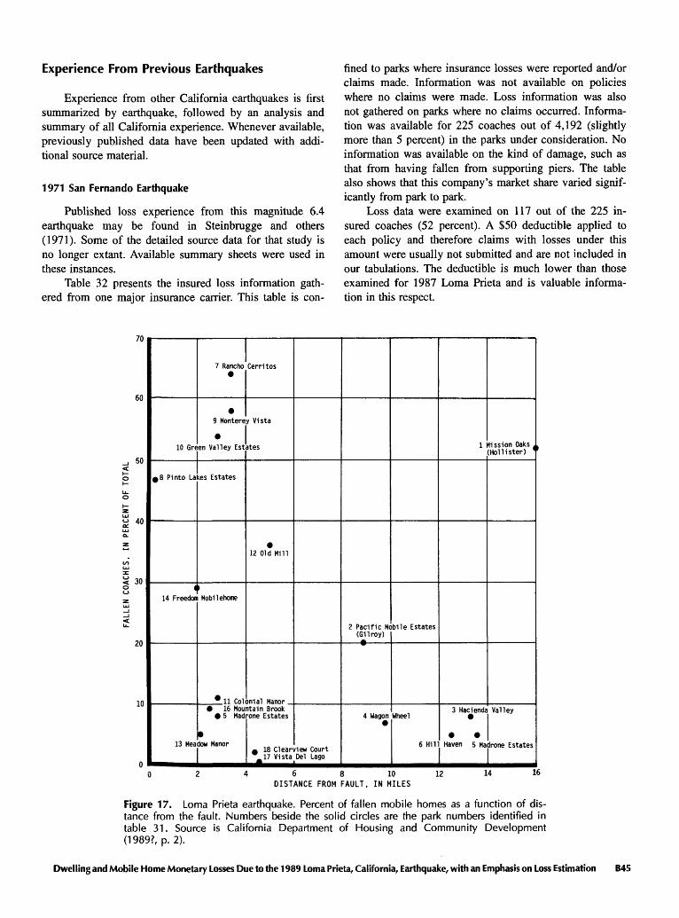
Experience From Previous Earthquakes

Experience from other California earthquakes is first summarized by earthquake, followed by an analysis and summary of all California experience. Whenever available, previously published data have been updated with addi­ tional source material.

1971 San Fernando Earthquake

Published loss experience from this magnitude 6.4 earthquake may be found in Steinbrugge and others (1971). Some of the detailed source data for that study is no longer extant. Available summary sheets were used in these instances.

Table 32 presents the insured loss information gath­ ered from one major insurance carrier. This table is con­

fined to parks where insurance losses were reported and/or claims made. Information was not available on policies where no claims were made. Loss information was also not gathered on parks where no claims occurred. Informa­ tion was available for 225 coaches out of 4,192 (slightly more than 5 percent) in the parks under consideration. No information was available on the kind of damage, such as that from having fallen from supporting piers. The table also shows that this company's market share varied signif­ icantly from park to park.

Loss data were examined on 117 out of the 225 in­ sured coaches (52 percent). A $50 deductible applied to each policy and therefore claims with losses under this amount were usually not submitted and are not included in our tabulations. The deductible is much lower than those examined for 1987 Loma Prieta and is valuable informa­ tion in this respect.

70

60

50

40

30

20

10

10 Gr«

98 Pinto La

<14 Freedoi

13 Mea

7 Rancho

9 Montere

en Valley Est

;es Estates

> Mobil ehome

11 Col 16 Mou 5 Mad

low Manor

Cerritos

y Vista

ites

12 Old Mill

inial Manorntain Brook one Estates

m 18 Clean ^17 Vista

Mew Court Del Lago

2 Pacific Me (Gilroy)

4 Wagon

bile Estates

Wheel

6 Hil

1

3 Hacienda

Haven 5 Ma

lission Oaks . (Hollister) '

Valley

Irone Estates

6 8 10 DISTANCE FROM FAULT, IN MILES

12 14 16

Figure 17. Loma Prieta earthquake. Percent of fallen mobile homes as a function of dis­ tance from the fault. Numbers beside the solid circles are the park numbers identified in table 31. Source is California Department of Housing and Community Development (1989?, p. 2).

Dwelling and Mobile Home Monetary Losses Due to the 1989 Loma Prieta, California, Earthquake, with an Emphasis on Loss Estimation B45

Table 32. Mobile home loss experience from 1971 San Fernando earthquake, mag­ nitude 6.4.

[Only parks with submitted insurance claims. Loss data provided by one major insurance carrier-.]

Insured Loss

Park No.

1234567891011121314151617/181920212223242526272829303132333435

City or Community

ChatsworthChatsuorthChatsworthCanoga ParkCanoga ParkCanoga ParkNorthridgeNorthridgeSylmarSylmarSylmarMission HillsMission Hi I IsSun ValleyPacoimaPacoimaPacoimaPacoimaSun I andSun I andNewhallNewhallSaugusSaugusSaugusSaugusSaugusSaugusSaugusSaugusSaugusSaugusSaugusSi mi Valley

Totals

Park Name

Indian HillsChatsworthImperial GardensCanoga CountryKona KaiEatonWalnutNorthridgeTahiti anSylmarLumarkMonterey ManorMission ManorLaurel CanyonShelter IsleShadow HillsBlue Star/MissionSkyland TerraceSherman GroveMonte VistaMulberry ParkPolynesianParklaneCordovaGranada VillaDesert GardensSierra TrailerRoyal OaksCaravillaBlackburnsSand CanyonCanyon BreezeLilly of ValleySanta Susana

Total Coaches In Park1

138198184155116111621681756610171956026096

240697671108144330280926076858450709011299

4,192

Insured Coaches In Park

8141212111241211410936231358626923357224105

225

DataCoaches

With Loss Over $50

12435319114761321132241782335412231

117

Average Percent Loss

0.01.66.73.23.62.06.65.2

30.025.419.78.019.811.37.75.413.539.13.511.67.014.620.123.17.47.88.69.99.97.58.30.08.52.1

on the number of spaces available for mobile homes. Parks are normally at or close to capacity. As a result, the number of coaches are slightly overstated for some parks.

Earthquake bracing in any form was very rare.Figure 18 shows the locations of all but two of the

mobile home parks for which loss data were available; park 35 in Simi Valley is slightly west of the map bound­ ary, and the other park (not listed in table 32) is in Gar- dena, about 35 miles from the source of the earthquake's energy, where a 24 percent loss occurred to one of fifty coaches. Undoubtedly there were many mobile home parks between 10 miles (park 35 in Simi Valley) and 35 miles (Gardena) with very small damage and no reported insurance claims. The Gardena loss was not considered to be meaningful and was not included in further study.

Thrust faulting, such as that which occurred during the 1971 San Fernando earthquake, creates ground frac­ tures and other surface disturbances over a wide zone (Barrows and others, 1973; Steinbrugge and others, 1971). Ground fractures and displacements scattered intensified damage to wood frame dwellings as shown in figure 14 of Steinbrugge and Algermissen (1990). They also intensified damage in the mobile home tracts.

Figure 19 plots percent losses against distance from the earthquake's energy source. The loss in the percent loss computations includes a $50 deductible. The park's distance is not from the epicenter, but rather from the energy release

B46 Estimation of Earthquake Losses to Housing in California

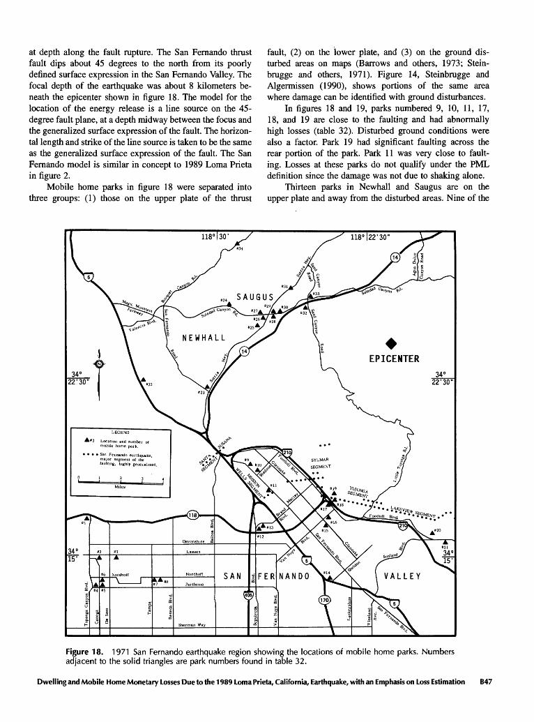
at depth along the fault rupture. The San Fernando thrust fault dips about 45 degrees to the north from its poorly defined surface expression in the San Fernando Valley. The focal depth of the earthquake was about 8 kilometers be­ neath the epicenter shown in figure 18. The model for the location of the energy release is a line source on the 45- degree fault plane, at a depth midway between the focus and the generalized surface expression of the fault. The horizon­ tal length and strike of the line source is taken to be the same as the generalized surface expression of the fault. The San Fernando model is similar in concept to 1989 Loma Prieta in figure 2.

Mobile home parks in figure 18 were separated into three groups: (1) those on the upper plate of the thrust

fault, (2) on the lower plate, and (3) on the ground dis­ turbed areas on maps (Barrows and others, 1973; Stein- brugge and others, 1971). Figure 14, Steinbrugge and Algermissen (1990), shows portions of the same area where damage can be identified with ground disturbances.

In figures 18 and 19, parks numbered 9, 10, 11, 17, 18, and 19 are close to the faulting and had abnormally high losses (table 32). Disturbed ground conditions were also a factor. Park 19 had significant faulting across the rear portion of the park. Park 11 was very close to fault­ ing. Losses at these parks do not qualify under the PML definition since the damage was not due to shaking alone.

Thirteen parks in Newhall and Saugus are on the upper plate and away from the disturbed areas. Nine of the

San Fernando earthquake, major segment of the faulting, highly generalized.

Figure 18. 1971 San Fernando earthquake region showing the locations of mobile home parks. Numbers adjacent to the solid triangles are park numbers found in table 32.

Dwelling and Mobile Home Monetary Losses Due to the 1989 Loma Prieta, California, Earthquake, with an Emphasis on Loss Estimation B47

thirteen are concentrated in a 4 mile stretch along, or close to, the Soledad Canyon Road. This road closely follows the Santa Clara River. Park 25, in a former flood plain of this river, sustained abnormally high losses, an average of 23 percent per unit. Several of the nine parks near the Santa Clara River were located on the unconsolidated gravels and sands of its flood plain. Nearly 95 percent of the coaches were shaken off their supports in park 26, while park 24, about a mile and a half away, experienced displacement of 280 coaches. It is likely that soil condi­ tions increased the losses, similar to Mission Oaks Park in the 1989 Loma Prieta earthquake (table 26).

Observations on San Fernando

Figure 19, a plot of losses versus fault distance, is of interest for the loss attenuation component in loss estima­

tion programs. This will be further examined in a follow­ ing section.

Table 33 shows a loss breakdown by construction com­ ponents as a percentage of value. Excluded are coaches located in disturbed ground areas and parks with incomplete loss breakdowns. This kind of information is useful for visual loss estimation purposes during field inspections.

Three mobile home parks (9,10,11) were adjacent to or in areas where losses for conventional dwellings have been determined see figure 18 herein along with figure 14 in Steinbrugge and Algermissen (1990). The right hand column in table 34 is the ratio between the average loss for mobile homes to wood frame dwellings. These ratios indicate that a San Fernando type earthquake may produce 2 to 4 times more damage to a mobile home than to a conventional wood frame dwelling in the more heavily shaken areas. These comparisons are at zero deductible, that is, at PML values.

45

40

35

30

25

20

15

10

23 ^

9

10 O

k

O11

O 17/18

<

A16

20

25A

13 '

'21

* 27* 22 26*

A 1 24

32

12 A

33

« D1st0 in t

. Lowe(San

A UPPCA (Sau

14

A31 3* <

<

1

urbed ground and/or 1 he near vicinity.

r plate of thrust fai Fernando Valley)

r plate of thrust fai gus and Newhall)

>7

8

2

A 34

*4 5

Suiting

Jit

lit

< 35

O QL

OZ3 O

Oot.

>- _l _l<

0000LU

00 00 O

345678

DISTANCE FROM SEISMIC ENERGY SOURCE, IN MILES

10 11

Figure 19. 1971 San Fernando earthquake. Percent loss over deductible as a function of distance for individual mobile home parks. Numbers are park numbers identified in table 32.

B48 Estimation of Earthquake Losses to Housing in California

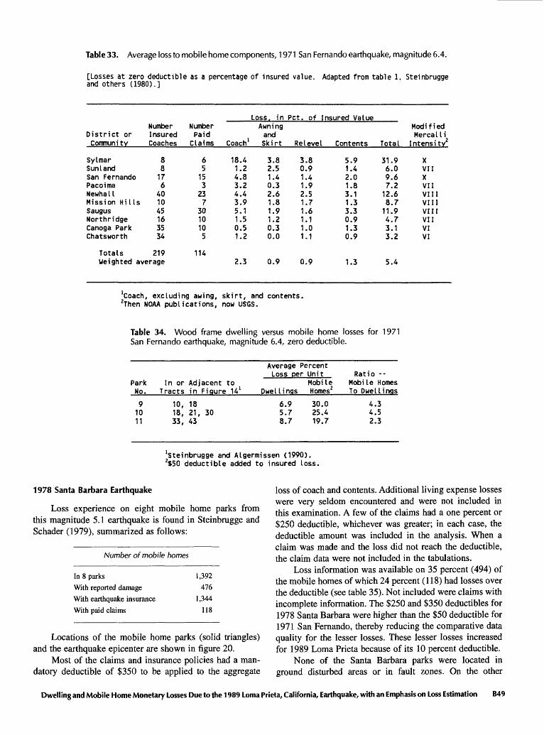
Table 33. Average loss to mobile home components, 1971 San Fernando earthquake, magnitude 6.4.

[Losses at zero deductible as a percentage of insured value. Adapted from table 1. Steinbrugge and others (1980).]

Loss, in

District orCommunity

SylmarSun I andSan FernandoPacoimaNewhallMission Hi UsSaugusNorthridgeCanoga ParkChatsworth

NumberInsuredCoaches

88176

401045163534

NumberPaid

Claims

65

153

237

3010105

Coach 1

18.41.24.83.24.43.95.11.50.51.2

AwningandSkirt

3.82.51.40.32.61.81.91.20.30.0

Pet. of Insured Value

Re I eve I

3.80.91.41.92.51.71.61.11.01.1

Contents

5.91.42.01.83.11.33.30.91.30.9

Total

31.96.09.67.212.68.711.94.73.13.2

ModifiedMercalli

Intensity2

XVIIXVIIVIIIVIIIVIIIVIIVIVI

Totals 219 Weighted average

1142.3 0.9 0.9 1.3 5.4

excluding awing, skirt, and contents. Then NOAA publications, now USGS.

Table 34. Wood frame dwelling versus mobile home losses for 1971 San Fernando earthquake, magnitude 6.4, zero deductible.

Average Percent

ParkNo.

91011

In or Adjacent toTracts in Figure 14 1

10, 1818, 21, 3033, 43

Loss per

Dwellings

6.95.78.7

UnitMobileHomes2

30.025.419.7

Ratio --Mobi le HomesTo Dwellings

4.34.52.3

Steinbrugge and Algermissen (1990). 2$50 deductible added to insured loss.

1978 Santa Barbara Earthquake

Loss experience on eight mobile home parks from this magnitude 5.1 earthquake is found in Steinbrugge and Schader (1979), summarized as follows:

Number of mobile homes

In 8 parks

With reported damage

With earthquake insurance

With paid claims

1,392

476

1,344

118

Locations of the mobile home parks (solid triangles) and the earthquake epicenter are shown in figure 20.

Most of the claims and insurance policies had a man­ datory deductible of $350 to be applied to the aggregate

loss of coach and contents. Additional living expense losses were very seldom encountered and were not included in this examination. A few of the claims had a one percent or $250 deductible, whichever was greater; in each case, the deductible amount was included in the analysis. When a claim was made and the loss did not reach the deductible, the claim data were not included in the tabulations.

Loss information was available on 35 percent (494) of the mobile homes of which 24 percent (118) had losses over the deductible (see table 35). Not included were claims with incomplete information. The $250 and $350 deductibles for 1978 Santa Barbara were higher than the $50 deductible for 1971 San Fernando, thereby reducing the comparative data quality for the lesser losses. These lesser losses increased for 1989 Loma Prieta because of its 10 percent deductible.

None of the Santa Barbara parks were located in ground disturbed areas or in fault zones. On the other

Dwelling and Mobile Home Monetary Losses Due to the 1989 Loma Prieta, California, Earthquake, with an Emphasis on Loss Estimation B49

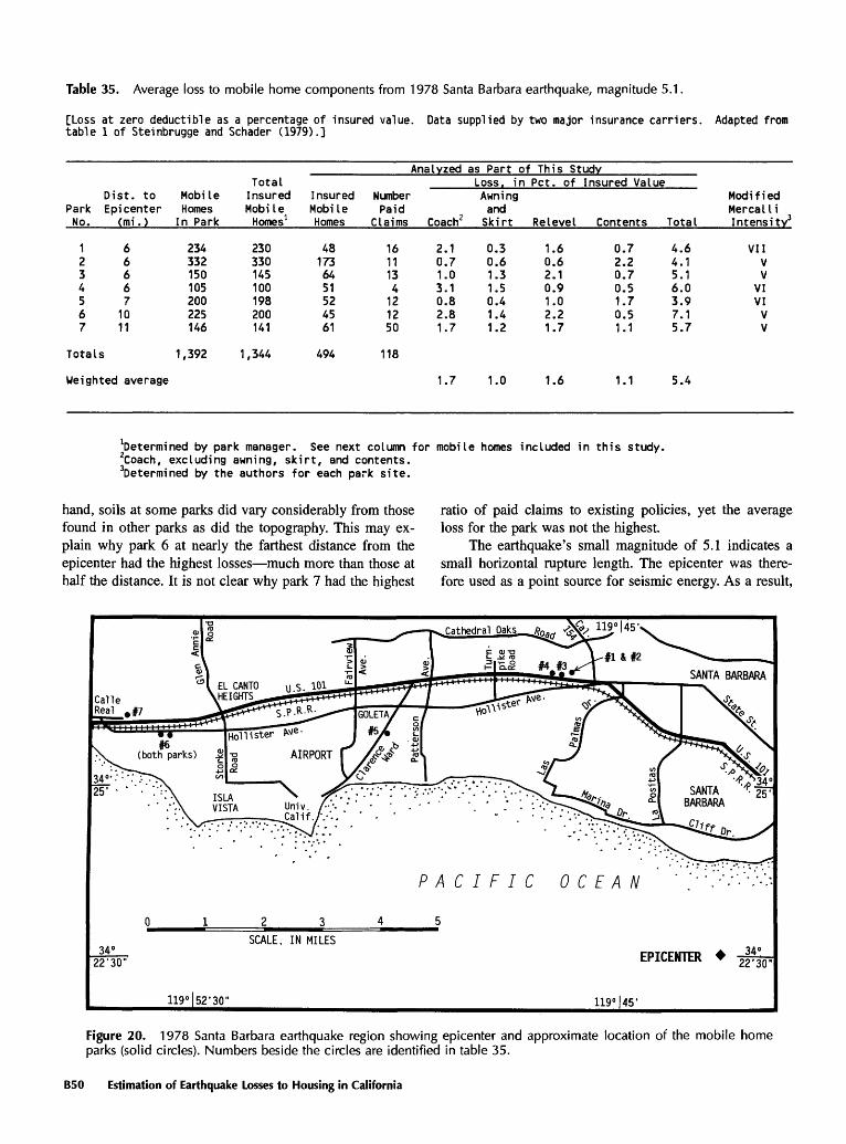
Table 35. Average loss to mobile home components from 1978 Santa Barbara earthquake, magnitude 5.1.

[Loss at zero deductible as a percentage of insured value. Data supplied by two major insurance carriers. Adapted from table 1 of Steinbrugge and Schader (1979).]

Analyzed as Part of This Study

Park No.

1234567

Dist. toEpicenter

(mi.)

666671011

MobileHomes

In Park

234332150105200225146

Total InsuredMobile Homes1

230330145100198200141

Loss, in Pet. of Insured ValueInsuredMobile Homes

481736451524561

NumberPaid

Claims

1611134121250

Coach2

2.10.71.03.10.82.81.7

Awningand Skirt

0.30.61.31.50.41.41.2

Re I eve I

1.60.62.10.91.02.21.7

Contents

0.72.20.70.51.70.51.1

Total

4.64.15.16.03.97.15.7

ModifiedMercalli Intensity3

VIIVV

VIVIVV

Totals 1,392

Weighted average

1,344 494 118

1.7 1.0 1.6 1.1 5.4

Determined by park manager. See next column for mobile homes included in this study. 2Coach, excluding awning, skirt, and contents. Determined by the authors for each park site.

hand, soils at some parks did vary considerably from those ratio of paid claims to existing policies, yet the average found in other parks as did the topography. This may ex- loss for the park was not the highest, plain why park 6 at nearly the farthest distance from the The earthquake's small magnitude of 5.1 indicates a epicenter had the highest losses much more than those at small horizontal rupture length. The epicenter was there- half the distance. It is not clear why park 7 had the highest fore used as a point source for seismic energy. As a result,

PACIFIC OCEAN

34° 22'30"

SCALE, IN MILES

EPICENTER

119°|52'30" 119°|45'

Figure 20. 1978 Santa Barbara earthquake region showing epicenter and approximate location of the mobile home parks (solid circles). Numbers beside the circles are identified in table 35.

B50 Estimation of Earthquake Losses to Housing in California

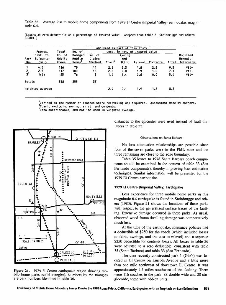
Table 36. Average loss to mobile home components from 1979 El Centre (Imperial Valley) earthquake, magni­ tude 6.4.

[Losses at zero deductible as a percentage of insured value. Adapted from table 3. Steinbrugge and others (1980).]

Analyzed as Part of This StudyApprox.

Dist. toPark EpicenterNo. (mi.)

1 4.52 2.533 1<?>

Totals

Weighted average

TotalNo. ofMobileHomes

11611785

318

No. ofDamagedMobileHomes 1

7910076

255

Loss, in Pet. of InsuredNo. ofClaimsStudied

14185

37

Coach2

2.62.21.4

2.4

AwningandSkirt

2.32.01.4

2.1

Re I eve I

1.81.92.6

1.9

Value

Contents

2.81.00.0

1.8

Total

9.57.15.4

8.2

ModifiedMercalliIntensity

VI 1+VII+VII+

Defined as the number of coaches where reIeve I ing was required. Assessment made by authors. 2Coach, excluding awning, skirt, and contents. 3Data questionable, and not included in weighted average.

Figure 21. 1979 El Centre earthquake region showing mo­ bile home parks (solid triangles). Numbers by the triangles are park numbers identified in table 36.

distances to the epicenter were used instead of fault dis­ tances in table 35.

Observations on Santa Barbara

No loss attenuation relationships are possible since four of the seven parks were in the PML zone and the three remaining are close to the zone boundary.

Table 35 losses to 1978 Santa Barbara coach compo­ nents should be examined in the context of table 33 (San Fernando components), thereby improving loss estimation techniques. Similar information will be presented for the 1979 El Centro earthquake.

1979 El Centro (Imperial Valley) Earthquake

Loss experience for three mobile home parks in this magnitude 6.4 earthquake is found in Steinbrugge and oth­ ers (1980). Figure 21 shows the locations of these parks with respect to the generalized surface traces of the fault­ ing. Extensive damage occurred in these parks. As usual, observed wood frame dwelling damage was comparatively much less.

At the time of the earthquake, insurance policies had a deductible of $250 for the coach (which included losses to skirts, awnings, and the cost to relevel) and a separate $250 deductible for contents losses. All losses in table 36 were adjusted to a zero deductible, consistent with table 35 (Santa Barbara) and table 33 (San Fernando).

The then recently constructed park 1 (Gio's) was lo­ cated in El Centro on Lincoln Avenue and a little more than one mile northwest of downtown El Centro. It was approximately 4.5 miles southwest of the faulting. There were 116 coaches in the park: 88 double-wide and 28 sin­ gle-wide, some with add-on units.

Dwelling and Mobile Home Monetary Losses Due to the 1989 Loma Prieta, California, Earthquake, with an Emphasis on Loss Estimation B51

Park 2 (KOA Country Life) was also of relatively new construction. There were 117 new coaches, all appearing to be supported on steel piers. The park contained 49 double- wide and 68 single-wide coaches. The park's location was east of El Centro on Ross Road near State Route 111. This location is approximately 2.5 miles southwest of the fault trace. Despite apparent severe shaking, pavements and con­ crete parking slabs in the park were undamaged. Nearby wood frame dwellings appeared undamaged.

Park 3 (Tangerine Gardens), with 85 coaches, was lo­ cated 3 miles south of downtown Brawley on Legion Road. It consisted of 42 double-wide and 43 single-wide coaches, with some being older than those found in the other parks. The location was approximately 1 mile northwest from a zone of fresh cracking on a pre-existing fault scarp.

Table 36 is similar to table 33 for San Fernando and to table 35 for Santa Barbara. Previous comments also apply here.

Test of Rapid Loss Estimation, El Centro

The time necessary to acquire loss data from insur­ ance sources is very long and the process can be tedious. There is usually a long wait during the insurance adjust­ ment period, including the settlement of difficult claims, and the company's processing time toward the last com­ pleted and closed claim. It is often desirable to make a quick postearthquake field survey of damage to develop an estimated aggregate loss.

A pilot method used for this earthquake was a word grading system which summarized observed damage and assigned percentage losses to these word gradings. The def­ initions of degrees of damage are found in Appendix B, and these definitions can be supplemented by representative photographs. The observed damage to skirt and awnings, coaches off or partially off supports, and needs for relevel- ing were quickly determined. The location of coaches in each park can be noted by space numbers usually available from the park manager's coach location map. This check allowed for future correlation with adjusters' information.

All coaches in the three parks in table 36 were exter­ nally inspected using the damage descriptions in Appendix B. Insurance loss data were then correlated with field ob­ servations in all three parks. Damage descriptions in Ap­ pendix B showed in table 37 the relationships to percent

Table 37. Mobile home damage from 1979 El Centro (Imperial Valley) earth­ quake, magnitude 6.4.

Coach damage

NoneSlightModerateSevere

Number of Coaches

365

23

Percent Loss

2.22.45.010.8

loss. The column "Percent Loss" is based on insurance loss (including contents) to insured value. Where there was no observed coach damage, any loss would be due to contents falling.

1980 Livermore (Greenville) Earthquakes

Two mobile home parks were in the more heavily shaken area of two earthquakes which occurred one day apart. Figure 22 is a vicinity map showing the location of these parks and also the approximate locations of some of the ground breakage associated with possible faulting. "The surface faulting was discontinuous .... and in places was difficult to separate from downslope gravity move­ ments .... and may have extended as far as the vicinity of Interstate Highway 580... "(Bonilla and others, 1980, p. 15). Magnitudes were, respectively, 5.5 and 5.6. Park 1 (Sunrise) was located northeast of Livermore and immedi­ ately north of Interstate 580 in the community of Spring- town. Every coach was exterior inspected in accordance with the methods given in Appendix B. Damage of some kind was almost universal to the coaches. Insured values were obtained from insurance sources, but no followup was made to obtain the results of adjusted claims. A sum­ mary of the field inspections is given in table 38.

Park 2 (Vineyard Mobile Villa), located 3 miles west of park 1 and also on Interstate 580, received no damage to any of its 159 coaches mostly single-wide. Park occu­ pants reported 5 to 10 percent of their shelf items fell. The damage contrast between these two parks was remarkable and was not attributed to construction.

Two story wood frame apartment houses adjacent to park 1 were interior and exterior inspected for comparison

Figure 22. 1980 Livermore (Greenville) earthquake region showing approximate location of surface breakage associated with faulting. Numbers by the solid triangles are park num­ bers identified in the text.

B52 Estimation of Earthquake Losses to Housing in California

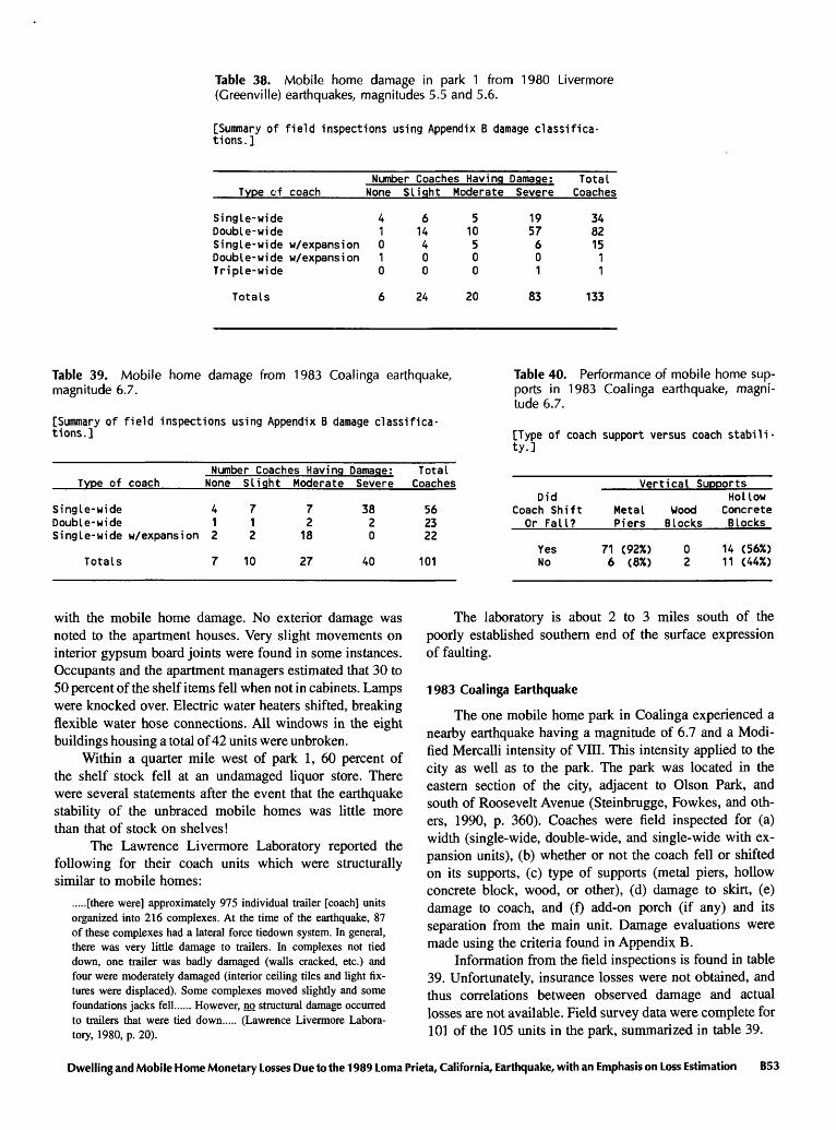
Table 38. Mobile home damage in park 1 from 1980 Livermore (Greenville) earthquakes, magnitudes 5.5 and 5.6.

[Summary of field inspections using Appendix B damage classifica­ tions.]

Number CoachesType of

Single-wideDouble-wideSingle-wideDouble-wideTriple-wide

coach

w/ expansionw/expansion

None

41010

HavingSlight Moderate

614400

510500

Damage:Severe

1957601

Total Coaches

348215

11

Totals 24 20 83 133

Table 39. Mobile home damage from 1983 Coalinga earthquake, magnitude 6.7.

[Summary of field inspections using Appendix B damage classifica­ tions.]

Number Coaches HavingType of

Single-wideDouble- wideSingle- wide

coach

w/expansion

None

412

Slight

712

Moderate

72

18

Damage:Severe

3820

TotalCoaches

562322

Totals 10 27 40 101

Table 40. Performance of mobile home sup­ ports in 1983 Coalinga earthquake, magni­ tude 6.7.

[Type of coach support versus coach stabili­ ty.]

Vertical SupportsDid

Coach Shift Or Fall?

YesNo

Metal Piers

71 (92%) 6 (8%)

Wood Blocks

0 2

Hollow Concrete Blocks

14 (56%) 11 (44%)

with the mobile home damage. No exterior damage was noted to the apartment houses. Very slight movements on interior gypsum board joints were found in some instances. Occupants and the apartment managers estimated that 30 to 50 percent of the shelf items fell when not in cabinets. Lamps were knocked over. Electric water heaters shifted, breaking flexible water hose connections. All windows in the eight buildings housing a total of 42 units were unbroken.

Within a quarter mile west of park 1, 60 percent of the shelf stock fell at an undamaged liquor store. There were several statements after the event that the earthquake stability of the unbraced mobile homes was little more than that of stock on shelves!

The Lawrence Livermore Laboratory reported the following for their coach units which were structurally similar to mobile homes:

.....[there were] approximately 975 individual trailer [coach] unitsorganized into 216 complexes. At the time of the earthquake, 87 of these complexes had a lateral force tiedown system. In general, there was very little damage to trailers. In complexes not tied down, one trailer was badly damaged (walls cracked, etc.) and four were moderately damaged (interior ceiling tiles and light fix­ tures were displaced). Some complexes moved slightly and some foundations jacks fell...... However, no. structural damage occurredto trailers that were tied down..... (Lawrence Livermore Labora­ tory, 1980, p. 20).

The laboratory is about 2 to 3 miles south of the poorly established southern end of the surface expression of faulting.

1983 Coalinga Earthquake

The one mobile home park in Coalinga experienced a nearby earthquake having a magnitude of 6.7 and a Modi­ fied Mercalli intensity of VIII. This intensity applied to the city as well as to the park. The park was located in the eastern section of the city, adjacent to Olson Park, and south of Roosevelt Avenue (Steinbrugge, Fowkes, and oth­ ers, 1990, p. 360). Coaches were field inspected for (a) width (single-wide, double-wide, and single-wide with ex­ pansion units), (b) whether or not the coach fell or shifted on its supports, (c) type of supports (metal piers, hollow concrete block, wood, or other), (d) damage to skirt, (e) damage to coach, and (f) add-on porch (if any) and its separation from the main unit. Damage evaluations were made using the criteria found in Appendix B.

Information from the field inspections is found in table 39. Unfortunately, insurance losses were not obtained, and thus correlations between observed damage and actual losses are not available. Field survey data were complete for 101 of the 105 units in the park, summarized in table 39.

Dwelling and Mobile Home Monetary Losses Due to the 1989 Loma Prieta, California, Earthquake, with an Emphasis on Loss Estimation B53

Table 41. Mobile home loss over deductible in PML zone.

[Limited to coaches with paid losses.]

Percent Loss Over Percent DeductibleLoma Prieta Watsonville Loma Prieta PML 1971 PML Zone ZIP 95076 Excl. ZIP 95076 San Fernando MAG = 7.1 MAG = 7.1 MAG = 7.1 MAG = 6.4

263 Coaches 81 Coaches 182 Coaches 70 CoachesPet. Ded.

0123456789

1011121314151617181920

Coach Coach-*- Coach Coach* Coach Coach* Coach* Only Conts. Only Conts. Only Conts. Conts.

... .

... .

... .

... .

... .

... .

... .

... .

... .

. . .

. . .

. .

. . .

. . .

. . .

. . .

. . .

. . .

m m

, ,

f f

m 9

m u

. .

^ u

, ,

. .

4.67 1.43 7.88 2.06 3.38 14.32 1.31 7.24 1.87 3.15 14.01 1.20 6.69 1.68 2.94 1

11.2710.599.909.238.618.027.466.946.445.98

.17 5.53

.08 5.08

.01 4.653.74 1.11 6.17 1.53 2.76 0.94 4.273.49 1.04 5.69 1.42 2.61 0.88 3.943.27 0.97 5.26 1.33 2.47 0.82 3.643.05 0.91 4.85 1.24 2.33 0.77 3.362.86 0.85 4.51 1.16 2.19 0.73 3.122.68 0.80 4.20 1.09 2.07 0.68 2.902.53 0.74 3.94 1.03 1.96 0.63 2.702.39 0.69 3.69 0.96 1.86 0.58 2.51

1978 Santa Barbara MAG = 5.1 56 Coaches

Coach* Conts.

1.181.020.860.710.570.450.350.270.210.170.130.110.090.070.060.060.050.040.040.030.02

The kinds of vertical supports for the coaches were compared with damage in table 40. This comparison sug­ gests that hollow concrete block supports performed better than steel piers. This was strongly confirmed in the 1989 Loma Prieta earthquake where 64 percent of coaches on steel piers fell while only 12 percent with hollow concrete block supports fell (table 31).

Synthesis and Overview

To this point, partial analyses and findings have been made by individual earthquakes. In this section, these are synthesized and organized by subject rather than by earthquake.

PML Zone

The 6 mile (10 kilometer) boundary of the PML zone from the surface projection of the line source of the earth­ quake energy is a reasonable model for mobile homes (fig­ ures 15, 16, and 17) as well as for wood frame dwellings. The model uses the average of all losses in the PML zone, excluding geohazards; this average is the PML, expressed in percent or in dollars. It is likely that this model will be substantially changed and improved when better near-field loss and seismic data are eventually obtained.

Loss Over Deductible in the PML Zone

As is the case for wood frame dwellings, determining the loss over deductible for the PML zone has two neces­ sary requirements. The value of each mobile home in the entire study area (or insurance company's book of busi­ ness) must be known, whether a mobile home suffered losses or not. Second, the losses and deductibles, if any, must be known for each mobile home. The first criteria is met by all mobile homes included in table 41. Only data from the 1971 San Fernando and the 1978 Santa Barbara earthquake come adequately close to satisfying the second criteria with their average deductibles of 0.2 percent and 1.2 percent, respectively. In these latter two cases, the dol­ lar deductible was very low, being $50 for 1971 San Fernando and $250 or $350 for 1978 Santa Barbara.

Unfortunately, the 1979 Santa Barbara loss over de­ ductibles may be incorrect by a large amount. At the damage threshold of magnitude 5, experience indicates that the 6 mile PML boundary is too large. The Santa Barbara parks are at this 6 mile boundary and these data are not used.

With few variants, mobile home loss over deductible analysis follows that for wood frame dwellings. Table 41 shows all known loss over deductible information. Analy­ sis was restricted to the 1989 Loma Prieta PML zone (col­ umns 2 and 3) and to the 1971 San Fernando experience (column 8). The Loma Prieta PML zone was chosen for

B54 Estimation of Earthquake Losses to Housing in California

Table 42. Loss over deductible as a function of deductible, in percent.

[Uncertainty factor « 1. Applicable to mobile home coaches, excluding contents.]

Percent Deducti bl e

0123456789

1011121314151617181920

Magnitude5.00

0.500.460.430.400.370.340.320.290.270.250.230.210.200.180.170.160.150.140.130.120.11

5.25

1.611.491.381.281.191.101.020.940.870.810.750.690.640.590.550.510.470.440.400.370.35

5.50

2.732.522.342.162.001.861.721.591.471.361.261.171.081.000.930.860.800.740.680.630.59

5.75

3.843.553.293.052.822.612.422.242.081.921.781.651.531.411.311.211.121.040.960.890.83

6.00

4.954.584.253.933.643.373.122.892.682.482.302.131.971.821.691.561.451.341.241.151.07

6.25

6.065.615.204.824.464.133.823.543.283.042.812.602.412.232.071.921.771.641.521.411.30

6.50

7.186.656.155.705.284.894.534.193.883.593.333.082.852.642.452.272.101.941.801.671.54

6.75

8.297.687.116.586.105.645.234.844.484.153.843.563.303.052.832.622.422.252.081.931.78

7.00

9.408.718.067.476.916.405.935.495.084.714.364.043.743.463.212.972.752.552.362.182.02

7.25

10.519.749.028.357.737.166.636.145.695.274.884.524.183.873.593.323.082.852.642.442.26

7.50

11.6310.779.979.238.557.927.336.796.295.825.394.994.624.283.973.673.403.152.922.702.50

7.75

12.7411.8010.9210.129.378.688.037.446.896.385.915.475.074.694.354.023.733.453.202.962.74

8.00

13.8512.8311.8811.0010.199.438.748.097.496.946.425.955.515.104.724.384.053.753.473.222.98

8.25

14.9613.8612.8311.8811.0110.199.448.748.097.496.946.435.955.515.104.734.384.053.753.483.22

analysis over the Watsonville study area since geohazards were not as important for mobile homes as they were for wood frame dwellings. The 1971 San Fernando losses over deductible data are for coach plus contents; 1989 Loma Prieta breaks these down by coach and by coach plus contents. Plotting normalized coach plus contents data for Loma Prieta (column 3) and San Fernando (col­ umn 8) showed a good match. As a consequence, the shape of the San Fernando curve was used for Loma Pri­ eta. From there on, the methods used for wood frame dwellings were largely followed.

The San Fernando loss over deductible equation is based on column 8 of table 41:

San Fernando coaches plus contents: LD = 11.65912 e-°-0768237D

where

LD = percent loss over deductible, and

D = deductible in percent.

The variables have the same meaning as those for wood frame dwellings. The equations for the Loma Prieta earth­ quake become:

Loma Prieta coaches:LD = 9.845945 e-°-0768237 D (9)

and

Loma Prieta coaches plus contents: LD = 3.014925 e-°-0768237 D (10)

Next including a variable magnitude and a user-selected uncertainty factor as was done for wood frame dwellings:

Coaches only, for general use:LD = [4.450450 (M - 5) + 0.5] e-°-0768237 D

where

M = magnitude, and

F = user-selected uncertainty factor,

and for:

Coaches plus contents, for general use:LD = [1.197583 (M - 5) + 0.5] e-°-0768237 D

xF (11)

x F (12)

where LD may be user-limited to magnitude 7.75 in equa­ tions 11 and 12.

Table 42 shows loss over deductible as a function of the deductible in 0.25 percent increments for coaches only. This a counterpart to table 15 for wood frame dwellings.

Figure 23 graphically shows the loss over deductible for coaches and for coaches plus their contents. These curves are for a magnitude 7.75 earthquake.

Maximum Losses in the PML Zone

Table 43 shows maximum losses for four earth­ quakes, with differing magnitudes for three of them. The average loss for the upper 10 percent of mobile homes de­ creases with decreasing earthquake magnitude column 4 of table 43.

With rare exception, individual coach plus contents losses before the deductible are not expected to exceed 2/3 of their combined values when ensuing fire and geohaz­ ards are excluded.

Dwelling and Mobile Home Monetary Losses Due to the 1989 Loma Prieta, California, Earthquake, with an Emphasis on Loss Estimation B55

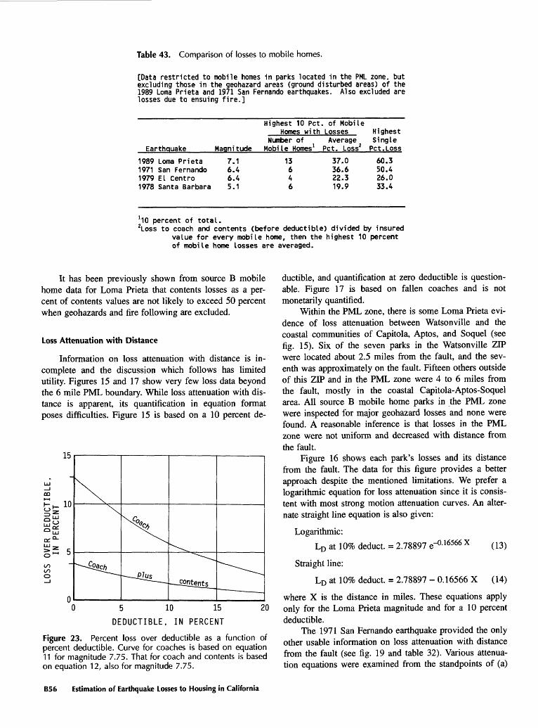
Table 43. Comparison of losses to mobile homes.

[Data restricted to mobile homes in parks located in the PML zone, but excluding those in the geohazard areas (ground disturbed areas) of the 1989 Loma Prieta and 1971 San Fernando earthquakes. Also excluded are losses due to ensuing fire.]

Highest 10 Pet. of Mobile Homes with Losses Highest

Earthquake Magnitude

1989 Loma Prieta1971 San Fernando1979 El Centre1978 Santa Barbara

7.16.46.45.1

Number of Mobile Homes

13646

Average 1 Pet. Loss2

37.036.622.319.9

Single Pet. Loss

60.350.426.033.4

J 10 percent of total.2Loss to coach and contents (before deductible) divided by insured

value for every mobile home, then the highest 10 percentof mobile home losses are averaged.

It has been previously shown from source B mobile home data for Loma Prieta that contents losses as a per­ cent of contents values are not likely to exceed 50 percent when geohazards and fire following are excluded.

Loss Attenuation with Distance

Information on loss attenuation with distance is in­ complete and the discussion which follows has limited utility. Figures 15 and 17 show very few loss data beyond the 6 mile PML boundary. While loss attenuation with dis­ tance is apparent, its quantification in equation format poses difficulties. Figure 15 is based on a 10 percent de-

15

10

0000o

0 5 10 15

DEDUCTIBLE, IN PERCENT

Figure 23. Percent loss over deductible as a function of percent deductible. Curve for coaches is based on equation 11 for magnitude 7.75. That for coach and contents is based on equation 12, also for magnitude 7.75.

ductible, and quantification at zero deductible is question­ able. Figure 17 is based on fallen coaches and is not monetarily quantified.

Within the PML zone, there is some Loma Prieta evi­ dence of loss attenuation between Watsonville and the coastal communities of Capitola, Aptos, and Soquel (see fig. 15). Six of the seven parks in the Watsonville ZIP were located about 2.5 miles from the fault, and the sev­ enth was approximately on the fault. Fifteen others outside of this ZIP and in the PML zone were 4 to 6 miles from the fault, mostly in the coastal Capitola-Aptos-Soquel area. All source B mobile home parks in the PML zone were inspected for major geohazard losses and none were found. A reasonable inference is that losses in the PML zone were not uniform and decreased with distance from the fault.

Figure 16 shows each park's losses and its distance from the fault. The data for this figure provides a better approach despite the mentioned limitations. We prefer a logarithmic equation for loss attenuation since it is consis­ tent with most strong motion attenuation curves. An alter­ nate straight line equation is also given:

Logarithmic:LD at 10% deduct. = 2.78897 e-°- 16566 x (13)

Straight line:

LD at 10% deduct. = 2.78897 - 0.16566 X (14)

where X is the distance in miles. These equations apply only for the Loma Prieta magnitude and for a 10 percent deductible.

The 1971 San Fernando earthquake provided the only other usable information on loss attenuation with distance from the fault (see fig. 19 and table 32). Various attenua­ tion equations were examined from the standpoints of (a)

B56 Estimation of Earthquake Losses to Housing in California

straight line versus exponential, (b) with or without the inclusion of parks located in the disturbed ground areas, (c) contiguous parks combined into one data entry, and other possibilities. It appears that a straight line function which excludes the parks in disturbed areas and also com­ bines contiguous parks will best represent reality up to 10 miles from the surface projection of the line source of seismic energy:

LD = 16.2986 - 1.3853 X (15)

where X is the distance in miles. This equation applies only to the San Fernando earthquake with its essentially zero deductible.

Earthquake Bracing

It is clearly evident that earthquake bracing systems are very effective. State certified systems have performed excellently, and none have been known to fail. There is no reason to believe that older pre-certification systems are necessarily inferior, but a qualified person such an engi­ neer should be the judge.

When no earthquake bracing is present, steel piers which support a coach are more likely to allow coach top­ pling than other types. On the other hand, steel piers as well as other types of vertical supports are expected to perform well upon installation of a certified earthquake bracing system, or equal as many seemed to be.

Coach Size and Damage

Coaches may be classified by size such as single- wide, double-wide, triple-wide, and with variants. Loma Prieta experience from 258 coaches showed that single- wide coaches performed marginally better than did two- or multiple-wide. The comparison was made on an average coach plus contents loss basis (7.0 and 7.8 percent, respec­ tively). In the 1980 Livermore earthquake (table 38), sin­ gle-wide performed better than double-wide "severe" damage. The reverse was true for the 1983 Coalinga earth­ quake (table 39). No doubt, the type of coach supporting piers is more important than coach size for unbraced coaches, but correlation data were unavailable.

No conclusions can be drawn from this mixed experi­ ence on coach size.

Loss Estimation From Rapid Field Inspections

The length of time needed to acquire insurance loss information may be excessive for many disaster response activities. The concept of a rapid field inspection introduced after the 1979 El Centro earthquake has promise. See tables 33 and 35 for information useful for field investigations.

The methodology has not gone beyond the pilot stage.

SUMMARY, MAJOR FINDINGS, AND CONCLUSIONS

Wood Frame Dwellings

Dwelling Loss Versus Other Losses

Within the nine county study area (fig. 1), wood frame dwelling losses amounted to 18.5 percent of the in­ sured economic loss (table 1). Clearly, wood frame dwell­ ing losses did not dominate over those to commercial and industrial properties.

In social and political senses, dwelling losses and dwelling habitability are of great importance to the general public, to disaster response entities such as the Red Cross, and to the Federal Emergency Management Agency and its state counterparts.

PML Zone and Modified Mercalli Intensities

Although damage extended throughout many counties around the San Francisco Bay, including those to the south around Monterey Bay (fig. 1), the heaviest shaken area was in the lightly inhabited regions within the Santa Cruz Mountains (fig. 3). This heaviest shaken area within 6 miles of the earthquake's energy release is defined as the PML zone shown in figure 3. The PML zone reasonably coincided with Modified Mercalli intensity VIE (fig. 14).

Average percentage losses within the MM VIE iso- seismal boundary can be estimated by losses within the PML zone (see below under "Deductibles)." Other studied earthquakes have had significantly different percent losses for this same intensity. In general, comparisons among earthquakes show poor correlations between intensities and actual losses.

Many regions within the United States do not have earthquake insurance loss data available. They may be many decades away from obtaining such information. Transferability of California loss experience to different geologic environments may involve great uncertainties. The use of intensities in dwelling loss estimation is useful only when suitable loss data are not available.

Dwelling Age and Loss

Dwellings constructed prior to 1940 suffered much more damage than did subsequent construction. This has also been observed in all California earthquakes since 1971. There was insufficient Loma Prieta data on older homes to adequately quantify comparisons. The most re­ cent quantified comparison was the 1983 Coalinga earth­ quake which showed that the pre-1940 wood frame dwellings had twice the percentage loss as did the more recent construction. There is some reason to believe that the Coalinga experience is not entirely applicable to the

Dwelling and Mobile Home Monetary Losses Due to the 1989 Loma Prieta, California, Earthquake, with an Emphasis on Loss Estimation B57

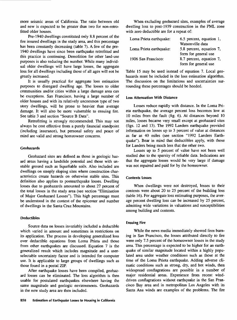
more seismic areas of California. The ratio between old and new is expected to be greater than two for non-retro­ fitted older houses.

Pre-1940 dwellings constituted only 8.8 percent of the fire insured dwellings in the study area, and this percentage has been constantly decreasing (table 7). A few of the pre- 1940 dwellings have since been earthquake retrofitted and this practice is continuing. Demolition for other land-use purposes is also reducing the number. While many individ­ ual older dwellings will have large losses, the aggregate loss for all dwellings including those of all ages will not be greatly increased.

It is usually practical for aggregate loss estimation purposes to disregard dwelling age. The losses to older communities and/or cities within a large damage area can be exceptions. San Francisco, having a large number of older houses and with its relatively uncommon type of two story dwellings, will be prone to heavier than average damage. It will also be more vulnerable to ensuing fire. See table 3 and section "Source B Data".

Retrofitting is strongly recommended. This may not always be cost effective from a purely financial standpoint (including insurance), but personal safety and peace of mind are valid and strong homeowner concerns.

Geohazards

Geohazard sites are defined as those in geologic haz­ ard areas having a landslide potential and those with un­ stable ground such as liquefiable soils. Also included are dwellings on steeply sloping sites where construction char­ acteristics create hazards on otherwise stable sites. This definition also applies to postearthquake losses. Dwelling losses due to geohazards amounted to about 27 percent of the total losses in the study area (see section "Elimination of Major Geohazard Losses"). This high percentage must be understood in the context of the epicenter and number of dwellings in the Santa Cruz Mountains.

Deductibles

Source data on losses invariably included a deductible which varied in amount and sometimes in restrictions on its application. The process in developing generalized loss over deductible equations from Loma Prieta and those from other earthquakes are discussed. Equation 7 is the generalized result which includes magnitude and a user- selectable uncertainty factor and is intended for computer use. It is applicable to large groups of dwellings such as those found in a postal ZIP.

After earthquake losses have been compiled, geohaz- ard losses can be eliminated. The loss algorithm is then usable for postulated earthquakes elsewhere having the same magnitude and geologic environments. Geohazards in the new study area are then included.

When excluding geohazard sites, examples of average dwelling loss to post-1939 construction in the PML zone with zero deductible are for a repeat of:

Loma Prieta earthquake:

Loma Prieta earthquake:

1906 San Francisco:

6.5 percent, equation 1, Watsonville data 5.8 percent, equation 7, form for general use 8.7 percent, equation 7, form for general use

Table 15 may be used instead of equation 7. Local geo­ hazards must be included in the loss estimation algorithm. The discussion on the limitations and uncertainties sur­ rounding these percentages should be heeded.

Loss Attenuation With Distance

Losses reduce rapidly with distance. In the Loma Pri­ eta earthquake, the average percent loss becomes low at 10 miles from the fault (fig. 6). At distances beyond 10 miles, losses became very small except at geohazard sites (figs. 12 and 13). The 1992 Landers earthquake provided information on losses up to 3 percent of value at distances as far as 40 miles (see section "1992 Landers Earth­ quake"). Bear in mind that deductibles apply, with those for Landers being much less that the other two.

Losses up to 5 percent of value have not been well studied due to the sparsity of reliable data. Indications are that the aggregate losses would be very large if damage was not repaired and paid for by the homeowner.

Contents Losses

When dwellings were not destroyed, losses to their contents were about 20 to 25 percent of the building loss (table 16). For aggregate loss estimating purposes, the aver­ age percent dwelling loss can be increased by 25 percent, admitting wide variations in valuations and susceptibilities among building and contents.

Ensuing Fire

While the news media immediately showed fires burn­ ing in San Francisco, the losses attributed directly to fire were only 7.5 percent of the homeowner losses in the study area. This percentage is expected to be higher for an earth­ quake of similar magnitude located within a highly popu­ lated area under weather conditions such as those at the time of the Loma Prieta earthquake. Adding adverse cli­ matic conditions such as strong, dry, and hot winds, then widespread conflagrations are possible in a number of major residential areas. Experience from recent wind- driven conflagrations without earthquake in the San Fran­ cisco Bay area and in metropolitan Los Angeles with its Santa Ana winds are examples of the problems. The fire

B58 Estimation of Earthquake Losses to Housing in California

departments were almost overwhelmed from these confla­ grations. With their added responsibilities after a great earthquake such as a repeat of 1906 San Francisco, the totality of the disaster is difficult to estimate. Fortunately, the simultaneous occurrence of a great earthquake and these severe climatic conditions has a very low probability.

Research Needs

The fundamental needs for improved predictive loss estimation require an improved integration of three major components:

(1) Actual loss statistics in place of the subjective Modified Mercalli intensities.

(2) Strong motion records for attenuation character­ istics which correlate with losses.

(3) Site or area quantification of geohazards which correlates with both of the above.

Subsequent algorithms should include other measurable quantities and clearly identified criteria which include magnitude, type of faulting, focal depth, characteristics of the energy release volume, and regional geology. Some work on this already exists and progress would likely be incremental over many years.

Nondwelling construction types are normally more complicated since the dynamic characteristics and the de­ sign/construction qualities are added variables.

Mobile Homes (Manufactured Housing)

Nonbraced Mobile Homes

Mobile homes which lack earthquake bracing are very vulnerable to falling off their supports. Within 20 miles of the Loma Prieta earthquake, about 25 percent of the approximately 2,500 mobile homes fell from their sup­ ports (table 31). Similar experience occurred in the 1971 San Fernando, 1978 Santa Barbara, 1979 El Centra, 1980 Livermore, and 1983 Coalinga earthquakes.

The percent of fallen mobile homes in nearby parks may vary by large margins. In the city of Watsonville which is in the PML zone, the percent of fallen coaches ranged from 5 to 64 percent, with the upper limit probably influ­ enced by a steep nearby slope (table 31 and fig. 7). However, the percent loss for the upper limit was only 17 percent. The reason is that once fallen, little additional damage is the general rule. This effectively put the maximum loss consid­ erably under the total loss for a fallen coach.

Earthquake Bracing

Commercially available earthquake bracing performed excellently. None of the 46 known mobile homes with

bracing fell from their supports (table 31). More limited experience in other earthquakes showed similar excellent results. While perfect performance is not to be expected in the future, there is certainly no doubt of the effectiveness of earthquake bracing.

Retrofitting mobile homes is quite simple, inexpen­ sive, and cost effective. It would seem reasonable public policy to require retrofitting or new bracing whenever ownership changes, a new mobile home is acquired, or one is moved to a new site.

Loss Attenuation

Excluding geohazards, percent losses for mobile homes per park were under 10 percent at 20 miles (fig. 16). This compares with 10 miles for wood frame dwell­ ings (fig. 5). A different loss attenuation algorithm is re­ quired for each.

Research Needs

The research needs for mobile homes are similar to those for wood frame dwellings but are not as needy or expensive. Emphasis should be placed on implementing retrofitting before spending time and resources on non- braced mobile homes.

Comparative Losses: Wood Frame and Mobile Homes

The 9.8 percent loss for Loma Prieta mobile homes is about twice the 5.3 percent for wood frame dwellings (equations 9 and 5, respectively). For 1971 San Fernando, table 34 shows that mobile homes were from 2 to 4 times more vulnerable to loss than were wood frame dwellings. This observation is limited to nonearthquake braced mo­ bile homes.

REFERENCES

Applied Technology Council, 1989, Field manual: postearth- quake safety evaluation of buildings: Redwood City, Califor­ nia, ATC-20-1, p. 114.

Barrows, A.G., Kahle, J.E., Weber, Jr., F.H., and Saul, R.B., 1973, Map of surface breaks resulting from the San Fernando, Cal­ ifornia, earthquake of February 9, 1971", in San Fernando, California, earthquake of February 9, 1971: NOAA, U.S. De­ partment of Commerce, v. 3, p. 127-135, plus map in pocket.

Benuska, L., ed., 1990, Loma Prieta earthquake reconnaissance report, in supplement to v. 6: Earthquake Spectra, May 1990.

Bonilla, M.G., Lienkaemper, J.J., and Tinsley, J.C., 1980, Surface faulting near Livermore, California, associated with the Jan­ uary, 1980, earthquake: U.S. Geological Survey Open-File Report 80-523.

California Department of Housing and Community Development, 1989(7), Evaluation of manufactured housing support system

Dwelling and Mobile Home Monetary Losses Due to the 1989 Loma Prieta, California, Earthquake, with an Emphasis on Loss Estimation B59

performance in the Loma Prieta earthquake: Sacramento, California, 14 p.

California Department of Insurance, 1981 [and annually thereaf­ ter], California earthquake zoning and probable maximum loss program: 54 p.

Cloud, W.K., and Perez, V., 1967, Accelerograms Parkfield earth­ quake: Seismological Society Bulletin, v. 57, p. 1179-1192.

Earthquake Engineering Research Institute, Newsletter, Septem­ ber, 1992: p. 6.

Housner, G.W., and Trifunac, M.D., 1967, Analysis of accelero­ grams Parkfield Earthquake: Seismological Society Bulle­ tin, v. 57, p. 1193-1220.

Kensler, C.D., 1985, The Morgan Hill earthquake of April 24, 1984 effects on mobile homes: Earthquake Spectra, v. 1, p. 607-613.

Lawrence Livermore Laboratory, 1980, The LLNL earthquake impact analysis committee report on the Livermore, Califor­ nia, earthquakes of January 24 and 26, 1980: Lawrence Liv­ ermore Laboratory, Univ. of Calif., Livermore, California, 107 p.

Lawson, A.C., ed., 1908, The California earthquake of 1906, re­ port of the State Earthquake Investigation Commission: Car­ negie Institution of Washington, 2 volumes plus atlas, Washington, D.C.

McNutt, S.R., and Toppozada, T.R., 1990, Seismological aspects of the 17 October 1989 earthquake, in The Loma Prieta (Santa Cruz Mountains), California earthquake of October 17, 1989: California Division of Mines and Geology, Special Publication 104, Sacramento, California.

Plafker, G., and Gallaway, J.P., eds., 1989, Lessons learned from the Loma Prieta, California, earthquake of October 17, 1989: U.S. Geological Survey Circular 1045, 48 p.

Steinbrugge, K.V., 1970, Engineering aspects of the Santa Rosa, California, earthquakes, October 1, 1969, in The Santa Rosa earthquakes of October 1, 1969: U.S. Coast and Geodetic Survey, ESSA, Dept. of Commerce, Washington, D.C.

Steinbrugge, K.V., 1986, Comment on the use and misuses of Modified Mercalli intensities, in Proceedings of Conference XXXII, Workshop on Future Directions in Evaluating Earth­ quake Hazards of Southern California: U.S. Geological Sur­ vey Open-File Report 86-401.

Steinbrugge, K.V., 1990, Earthquake losses to 1- to 4-family Cal­ ifornia dwellings: who pays?, in Hearings before the Sub­ committee on Policy Research and Insurance Committee on

Banking, Finance and Urban Affairs: House of Representa­ tives, Sept. 11 and 12, 1990, Serial No. 101-168, p. 798-808.

Steinbrugge, K.V., and Algermissen, S.T., 1990, Earthquake loss­ es to single-family dwellings: California experience: U.S. Geological Survey Bulletin 1939.

Steinbrugge, K.V., Algermissen, S.T., and Lagorio, H.J., 1984, Determining monetary losses and casualties for use in earth­ quake mitigation and disaster response planning, in Proceed­ ings, 8th World Conference on Earthquake Engineering, San Francisco, California, July 21-28, 1984: Prentice-Hall, v. VII, p. 615-622.

Steinbrugge, K.V., Bush, V.R., and Zacher, E.G., 1959, Damage to buildings and other structures by the San Francisco earth­ quake of March 22, 1957, in Oakeshott, Gordon B., ed., San Francisco earthquakes of March 1957: California Division of Mines, Special Report 57.

Steinbrugge, K.V., Fowkes, E.J., Lagorio, H.J., and Algermissen, S.T., 1990, Dwelling monetary losses, in The Coalinga, Cali­ fornia, earthquake of May 2, 1983: U.S. Geological Survey Professional Paper 1487.

Steinbrugge, K.V., Manning, J.H., and Degenkolb, H.J., 1967, Building damage in Anchorage, in The Prince William Sound, Alaska, earthquake of 1964 and aftershocks: ESSA, U.S. Department of Commerce, v. II, part A, p. 7-217, plus map in pocket.

Steinbrugge, K.V., and Schader, E.E., 1979, Mobile home dam­ age and losses, Santa Barbara earthquake, August 13, 1978: California Seismic Safety Commission, Sacramento, Califor­ nia, SSC 79-06, 19 p.

Steinbrugge, K.V., Schader, E.E., and Algermissen, ST., 1980, Mobile homes and earthquake damage in California: Califor­ nia Seismic Safety Commission, Sacramento, California, SSC 79-07, 29 p.

Steinbrugge, K.V., Schader, E.E., Bigglestone, H.C., and Weers, C.A., (n.d., but 1971), San Fernando earthquake, February 9, 1971: Pacific Fire Rating Bureau, San Francisco, California, 93 p., plus map in pocket.

Stover, C.W, and others, 1990, Preliminary isoseismal map for the Santa Cruz (Loma Prieta), California, earthquake of Oc­ tober 18, 1989, UTC: U.S. Geological Survey Open-File Re­ port 90-18.

Youd, T.L., and Perkins, J.B., 1987, Map showing liquefaction susceptibility of San Mateo County, California: U.S. Geologi­ cal Survey Miscellaneous Investigation Series, Map I-1257-G.

B60 Estimation of Earthquake Losses to Housing in California

APPENDIX A. SENSITIVITY: LOSS OVER DEDUCTIBLE VERSUS DWELLING PML CHANGES

The term "percent PML" is frequently misunderstood. For convenience, discussion found in Steinbrugge and Al- germissen (1990, p. A65) has been updated and repro­ duced here.

The commercial/industrial underwriters emphasize in­ dividual risks in their aggregate loss evaluations, whereas personal lines underwriters emphasize large numbers of risks. Commonly stated, the percent PML minus the per­ cent deductible is the percent loss over the deductible. In a mathematical sense:

(percent PML) - (percent deductible) = (percent loss over the deductible)

These terms may be rearranged:

(percent PML) = (percent loss over the deductible) + (percent deductible)

This latter form is used in the following discussion. The percent PML for wood frame dwellings is not a fixed value since it is always in the context of a deductible plus the loss over the deductible. For example, consider a dam­ aging earthquake during which 1,000 wood frame dwell­ ings in a small area are subjected to the same severe ground motion. First, assume that two dwellings are total losses and the others have losses distributed between 0 percent and 100 percent. With a 10 percent deductible and using the current State of California's 1.7 percent loss over this deductible, the result is an 11.7 percent PML. Next assume a highly improbable deductible of 95 percent. There still would be at least two dwelling losses over the 95 percent deductible. The percent PML for the 1,000 houses would therefore have to be the 95 percent deduct­ ible plus a very small loss over the deductible to reflect the two total losses plus any other losses between 95 per­ cent and 100 percent. In summary, the percent PML varies as a function of the percent deductible and may never be less than the percent deductible.

If the percent PML is close to the percent deductible as in the case for wood frame dwellings, the percent loss over the deductible is very sensitive to any change in the percent PML. Consider a 10 percent deductible with an 11.7 percent PML for wood frame dwellings. For $1 bil­ lion in wood frame dwelling liabilities, the loss over the deductible would be 1.7 percent of $1 billion, or $17 mil­ lion. On the other hand should the maximum credible earthquake actually produce a 12.7 percent PML instead of 11.5 percent, then the loss over the deductible would be 2.5 percent, or $25 million. In this case, a 1 percent in­ crease in the percent PML creates a 47 percent increase in the aggregate dollar PML.

APPENDIX B. DEFINITIONS OF DEGREE OF DAMAGE TO MOBILE HOMES

The following definitions of degree of damage require a physical inspection of each coach consisting of an exam­ ination of not less than the front and two sides. Except occasionally, interiors are not inspected. Minor exterior damage such as disturbed caulking and slightly bent skirt­ ing may escape observation from these rapid inspections.

Contents damage is usually not evaluated during these inspections. However, such information may be eventually obtained when the degree of coach damage is correlated with the closed insurance claims.

NONE is defined as a coach which has no visible ex­ terior damage upon a quick three-sided inspection of the unit. Often minor damage can be found during a detailed inspection which includes crawling under the unit.

SLIGHT damage is defined as a coach which has skirting damage principally on one side, indicating that relative minor movement took place. Skirting is normally metal although masonry or fiberboard are sometimes ob­ served. Replacement of the damaged portion of the skirt­ ing, slight releveling, and recaulking of roof seams at the joint line are the anticipated repairs.

MODERATE damage is defined as a coach which has skirting damage on several sides, and possibly on all sides. Releveling and caulking problems are significantly greater than for "slight" damage. Minor permanent offsets of the coach and porch may be observed upon careful inspection.

SEVERE damage is defined as a coach which is to­ tally or partially off its supports. Alternatively, the coach may have substantially shifted with respect to its supports which may be bent or rotated. Skirting is severely dam­ aged. Awnings and porches are damaged, with displace­ ments commonly observed between coaches and porches. Unobserved damage may include holes punched through the floor when the coach leaves its supports. We now be­ lieve that SEVERE should be divided into two categories: (1) partly off supports and (2) completely off supports.

The technique used in the past to apply these guidelines has been:

(1) For all parks within a reasonable distance from the earthquake, field inspect all coaches in each park using a damage classification system such as that found in Appendix B. If practical, a more sophisticated system should be used. From a time standpoint the surveys probably should be restricted to external inspections with interiors examined only when convenient.

(2) Determine from the mobile home park manager, or others, an estimate of the average value of each coach in the park on some consistent basis, such as the replacement value or current resale

Dwelling and Mobile Home Monetary Losses Due to the 1989 Loma Prieta, California, Earthquake, with an Emphasis on Loss Estimation B61

value. Preferably, the valuations should be on a classification system described in Appendix B issingle-wide, double-wide, and so forth basis. used.This should be eventually related to insured val- Refinements to this system can include type of foundationues and to paid claims in order to improve the such as steel or concrete piers, wood blocks, or hollowmethodology. concrete blocks. Data tabulation can include information

(3) Compute the loss using loss percentages such as on the bracing, if any, be it state certified or not. This lat-those found in previous sections if the damage ter refinement is the more important of the two.

B62 Estimation of Earthquake Losses to Housing in California

Tab

le 4

4.

Bui

ldin

g, c

onte

nts,

and

Ale

los

ses,

bef

ore

and

afte

r de

duct

ible

.

[See

text

und

er "

Dw

ellin

g Lo

sses

Bef

ore

and

Afte

r Ded

uctib

le"

for e

xpla

natio

n]

DATA F

ILE

STAT

E-6A

.DAT

DISTRIBUTION O

F BUILDING A

ND C

ONTENTS

LOSS

ES B

Y ZI

P DA

TA I

N ZI

P-FA

ULT

ORDE

R (C

olum

n 2)

ALAM

EDA,

CONTRA C

OSTA,

MARI

N. MONTEREY,

SAN

BENITO.

SAN

FRAN

CISC

O, SA

N MA

TED.

SA

NTA

CLAR

A, an

d SANTA

CRUZ C

ounties

ZIP

FAULT

ZIP

DIST.

(1)

95019

9507

6

9502

6

9504

4

9500

1

9500

3

9506

6

95073

9500

7

9500

6

9500

5

9506

5

95018

95030

95010

9504

1

9503

1

9506

1

95062

9503

2

95004

95070

95064

95060

95020

9514

1

93907

9512

0

95124

95130

(2) 2.0

2.1

2.7

2.7

3.5

3.5

3.9

4.3

4.6

4.7

4.8

5.3

5.5

5.7

5.9

5.9

6.5

7.5

7.5

7.6

8.3

8.5

8.6

8.9

9.6

9.6

10.0

10.0

10.0

10.0

<=mmu i

,uyt

K"»=

> «

DWEL

. CO

NTS.

NO.

VALUE

VALU

E

DWEL.

x$MT

l. x$

Mil.

(3) 14 422 1 5 1

475

294

165 11 216

159

129

156

883 62 13 1 1

273

576 42

1.37

2 2

504

489 1

186

1.79

8

1,096

322

(4) 1 58 0 0 0 76 47 26 1 29 21 20 19 188 8 2 0 0 33 114 5

313 0 76 72 0 24 321

149 39

(5)

1 42 0 0 0 57 35 19 1 21 15 15 13 141 6 1 0 0 24 87 4

237 0 56 54 0 18 243

112 30

:= P

AID

LOSS

UNDER E

Q COVER ==> <= P

AID

LOSS U

NDER

HO

COVER => <

NO.

PCT.

DWEL.

CONT

S.

ALE

NO.

PCT.

DW

EL.

CONT

S.

ALE

NO.

DWEL

. DWEL.

x$1000

x$1000 x

$100

0 DW

EL.

DWEL.

x$10

00

x$10

00 x

JlOO

O DWEL

(6) 3

150 1 3 1

201

115 81 2 92 62 59 66 348 16 0 0 0 72 70 5 85 0

132 45 0 11 52 20 6

(7)

21.4

35.5

100.

0

60.0

100.0

42.3

39.1

49.1

18.2

42.6

39.0

45.7

42.3

39.4

25.8 0.0

0.0

0.0

26.4

12.2

11.9 6.2

0.0

26.2 9.2

0.0

5.9

2.9

1.8

1.9

(8) 27

3,884 39 85 71

3,84

9

2,246

2,70

2 60

2,54

2

1,04

9

1.351

1.224

16.300 143 0 0 0

1.19

1

1,51

5 33

1.75

6 0

2.708

768 0

136

745

178 9

(9)

9

1,04

4 0 44 19 885

540

579 2

411

194

434

213

4,57

4 38 0 0 0

343

608 30 312 0

291

230 0 14 217 75 9

(10)

(11)

0

278 17 2 30 211

156

370 5

203 44 131

114

2.05

8 9 0 0 0 57 79 2

149 0

161 51 0 6 32 3 0

1 16 0 1 1 19 9 9 0 14 4 3 5 80 2 0 0 0 2 6 0 5 0 11 0 0 2 1 0 0

(12) 7.1

3.8

0.0

20.0

100.0

4.0

3.1

5.5

0.0

6.5

2.5

2.3

3.2

9.1

3.2

0.0

0.0

0.0

0.7

1.0

0.0

0.4

0.0

2.2

0.0

0.0

1.1

0.1

0.0

0.0

(13)

1

157 0 0 13 126

133 77 0

142 13 7 33

1.32

8 5 0 0 0 18 40 0 44 0 54 0 0 2 0 0 0

(14)

0 3 0 2 0 19 76 28 0 10 2 11 0

274 0 0 0 0 0 3 0 0 0 1 0 0 0 0 0 0

(15) 0 1 0 0 0 45 30 2 0 2 0 0 0 36 0 0 0 0 0 0 0 0 0 0 0 0 0 0 0 0

E

Q COVER

> < H

O COVER

> < E

O+HO C

OVER

-

NO.

NO.

. BLDG.

CONT

S.

ALE

DWEL

. BLDG.

CONT

S.

ALE

DWEL.

BLDG

. CONTS.

(16)

(1

7)

3

150 1 3 1

201

115 81 2 92 62 59 66 348 16 0 0 0 72 70 5 85 0

132 45 0 11 52 20 6

57

6,698 55 101

216

6.592

3,995

4,55

7 80

3,963

1,81

7

2.467

2,017

27.2

74 317 0 0 0

2,086

3,087 85

3,46

1 0

4.431

1.35

3 0

255

1,419

437 72

(18)

(19) (20)

9

1.04

4 0 44 19 885

540

579 2

411

194

434

213

4,574

2

38 0 0 0

343

608 30 312 0

291

230 0 14 217 75 9

0

278 17 2 30 211

156

370 5

203 44 131

114

,058 9 0 0 0 57 79 2

149 0

161 51 0 6 32 3 0

1 16 0 0 1 15 8 9 0 14 2 2 5 76 2 0 0 0 2 6 0 5 0 10 0 0 2 1 0 0

(21) 1

157 0 0 13 126

133 77 0

142 13 7 33 877 5 0 0 0 18 40 0 44 0 54 0 0 2 0 0 0

(22) 0 3 0 2 0 19 76 28 0 10 2 11 0

274 0 0 0 0 0 3 0 0 0 1 0 0 0 0 0 0

(23)

(2

4)

(25)

0 1 0 0 0 45 30 2 0 2 0 0 0 36 0 0 0 0 0 0 0 0 0 0 0 0 0 0 0 0

3

150 1 3 1

201

115 81 2 92 62 59 66 348 16 0 0 0 72 70 5 85 0

132 45 0 11 52 20 6

59

6.854 55 101

229

6.718

4.128

4.63

4 80

4.104

1,829

2.474

2.050

28,1

51 322 0 0 0

2.10

4

3.127 85

3,506 0

4.485

1.353 0

257

1,419

437 72

==>

ALE

(26)

(2

7)

9

1.046 0 45 20 903

616

607 2

421

196

445

213

4.848

2,

38 0 0 0

343

610 30 312 0

292

230 0 14 217 75 9

0

278 17 2 30 257

186

372 5

206 44 131

114

,094 9 0 0 0 57 79 2

149 0

161 51 0 6 32 3 0

<=DERIVED

DATA

=>

BLDG

. CONTS. AL

E

*LOSS

RATI

O RA

TIO

PO

(28)

(29)

(30)

(3

1)

4.0

0.16

1 0.007

FREE

DOM

11.8 0

.153 0

.041 W

ATSO

NVIL

LE

100.0

0.005

0.318

REDW

OOD

ESTA

TES

21.1 0

.449 0

.020 R

EDWO

OD E

STAT

ES

73.5 0

.086 0

.131 A

PTOS

8.9

0.134

0.038

APTOS

8.8

0.149

0.045

SANT

A CR

UZ

17.9 0

.131 0

.080 S

OQUEL

6.3

0.02

1 0.060

BROOKDALE

14.0 0

.103 0

.050 B

OULD

ER CREEK

8.6

0.107

0.024

BEN

LOMO

ND

12.1 0

.180 0

.053 S

ANTA

CRU

Z

10.8 0

.104 0

.056 F

ELTON

14.9 0

.172 0

.074

LOS G

ATOS

4.1

0.117

0.027

CAPI

TOLA

0.0

0.000

0.000

MOUNT

HERM

ON

0.0

0.000

0.000

LOS GA

TOS

0.0

0.000

0.000

SANT

A CR

UZ

6.4

0.163

0.027

SANTA

CRUZ

2.7

0.195

0.025

LOS GA

TOS

1.5

0.350

0.025

AROMAS

1.1

0.089

0.043

SARA

TOGA

0.0

0.000

0.000

SANTA

CRUZ

5.9

0.065

0.036

SANT

A CR

UZ

1.9

0.170

0.038

GILROY

0.0

0.000

0.000

SAN

JOSE

1.1

0.055

0.023

SALI

NAS

0.4

0.153

0.023

SAN

JOSE

0.3

0.172

0.006

SAN

JOSE

0.2

0.129

0.000

SAN

JOSE

Tabl

e 44

. B

uild

ine,

con

tent

s, a

nd A

le l

osse

s, b

efor

e an

d af

ter

de

du

ctib

le C

on

tinu

ed

DATA

FIL

E ST

ATE-

6A.D

AT

DIST

RIBU

TION

OF

BUILDING A

ND C

ONTENTS

LOSS

ES B

Y ZI

P DA

TA I

N ZI

P-FA

ULT

ORDE

R (Column

2)

ALAM

EDA,

CONTRA C

OSTA,

MARIN, MO

NTER

EY,

SAN

BENITO,

SAN

FRANCISCO, SA

N MATED. SA

NTA

CLAR

A, and

SANT

A CR

UZ C

ount

ies

ion

of

Earthi

jz 5" 5- I t/1 8" o era 5* n w 1 5*

ZIP

FAUL

T

ZIP

DIST

.

(1)

(2)

95008

10.2

95012

10.4

95129

10.8

95039

10.9

95118

11.1

95014

11.3

95017

11.5

95117

11.8

95123

12.6

95128

12.7

95037

12.9

95046

13.0

95125

13.0

95136

13.1

95119

13.2

94087

13.5

94024

13.7

95051

13.8

95126

13.8

95139

13.9

95050

14.3

95052

14.3

9511

4 14.4

95150

14.4

95157

14.4

95160

14.4

95045

14.5

9408

8 14

.7

95111

14.8

94022

14.9

<=EQ+HO C

OVE

DWEL

.

NO.

VALUE

CONTS. <

VALUE

DWEL

. x$Mil. x$Mil.

(3) 572 23

1,033 1

626

1.482 3

295

1,284

366

745 78 757

687

290

1,297 96 966

135

207

364 1 2 10 1 1 29 1

347

1.835

(4) 75 2

141 0 79 236 0 40 168 46 138 15 108 95 39 189 20 119 20 28 43 0 0 1 0 0 4 0 41 432

(5) 57 2

106 0 59 178 0 30 126 34 103 11 80 71 29 143 15 89 14 21 32 0 0 1 0 0 3 0 30 327

PAID L

OS

NO.

PCT.

DWEL.

(6) 13 1 31 0 7 77 0 12 35 5 41 8 50 20 9 9 6 34 4 2 6 0 0 0 0 0 1 0 4

127

DWEL

.

(7)

2.3

4.3

3.0

0.0

1.1

5.2

0.0

4.1

2.7

1.4

5.5

10.3 6.6

2.9

3.1

0.7

6.3

3.5

3.0

1.0

1.6

0.0

0.0

0.0

0.0

0.0

3.4

0.0

1.2

6.9

= AG

GREG

ATE

LOS!

iS UNDER

EQ C

OVEI

DWEL

. CONTS.

x$10

00

(8) 12

6 8

182 0 23 718 0

176

369

113

1.059 61

1,073

452 77 76 336

335 31 1 69 0 0 0 0 0 48 0 25

4,623

5ES AF

TER

DEDU

CTIB

LE

R => <= P

AID

LOS

ALE

NO.

PCT.

x$10

00 x

$100

0

(9) 23 0 88 0 4

303 0 21 70 22 140 44 52 9 31 74 17 51 2 3 18 0 0 0 0 0 21 0 8

1,611

(10)

36 2 2 0 0 19 0 4 16 0 57 0 47 29 1 0 0 7 0 0 3 0 0 0 0 0 31 0 1

456

DWEL

.

(11)

0 0 4 0 0 1 0 0 1 0 1 1 2 0 0 0 1 0 0 0 0 0 0 0 0 0 1 0 0 22

DWEL.

(12) 0.0

0.0

0.4

0.0

0.0

0.1

0.0

0.0

0.1

0.0

0.1

1.3

0.3

0.0

0.0

0.0

1.0

0.0

0.0

0.0

0.0

0.0

0.0

0.0

0.0

0.0

3.4

0.0

0.0

1.2

iS UN

DER

DWEL.

x$10

00

(13)

0 0 14 0 0 1 0 0 0 0 8 1 5 0 0 0 2 0 0 0 0 0 0 0 0 0 4 0 0

125

HO C

OVER

>

CONTS.

ALE

<=sa=s=

NO.

x$10

00 x

$1000

DWEL

.

(14)

0 0 0 0 0 0 0 0 0 0 1 0 0 0 0 0 0 0 0 0 0 0 0 0 0 0 0 0 0 4

(15) 0 0 0 0 0 0 0 0 0 0 0 0 0 0 0 0 0 0 0 0 0 0 0 0 0 0 0 0 0 0

(16)

13 1 31 0 7 77 0 12 35 5 41 8 50 20 9 9 6 34 4 2 6 0 0 0 0 0 1 0 4

127

= E

Q CO

VER =

BLDG

.

(17)

318 18

552 0

111

1,721 0

325

760

328

1,84

8

172

1,83

7

759

179

181

644

710 89 23 146 0 0 0 0 0

100 0 70

8,41

3

CONTS.

(18) 23 0 88 0 4

303 0 21 70 22 140 44 52 9 31 74 17 51 2 3 18 0 0 0 0 0 21 0 8

1,611

REGA

TE L

OSSE

S BE

FORE

DED

UCTI

BLE

x $1

1

====>

<-,

. HO

COV

ER M

M.. ,

...!..

,> <=

NO.

NO.

ALE

(19) 36 2 2 0 0 19 0 4 16 0 57 0 47 29 1 0 0 7 0 0 3 0 0 0 0 0 31 0 1

456

DWEL.

(20) 0 0 4 0 0 1 0 0 1 0 1 1 2 0 0 0 1 0 0 0 0 0 0 0 0 0 1 0 0 22

BLDG

.

(21) 0 0 14 0 0 1 0 0 0 0 8 1 5 0 0 0 2 0 0 0 0 0 0 0 0 0 4 0 0

125

CONTS.

(22) 0 0 0 0 0 0 0 0 0 0 1 0 0 0 0 0 0 0 0 0 0 0 0 0 0 0 0 0 0 4

ALE

(23) 0 0 0 0 0 0 0 0 0 0 0 0 0 0 0 0 0 0 0 0 0 0 0 0 0 0 0 0 0 0

DWEL

.

(24)

13 1 31 0 7 77 0 12 35 5 41 8 50 20 9 9 6 34 4 2 6 0 0 0 0 0 1 0 4

127

= EO

+HO CO

VER

BLDG

.

(25)

318 18

566 0

111

1,721 0

325

761

328

1.856

173

1.842

759

179

181

646

710 89 23 146 0 0 0 0 0

104 0 70

8,53

8

CONT

S.

(26) 23 0 88 0 4

303 0 21 70 22 141 44 52 9 31 74 17 51 2 3 18 0 0 0 0 0 21 0 8

1,614

==> <

=DERIVED D

ATA=

>

BLDG

. CONTS. AL

E

ALE

*LOS

S RA

TIO

RATI

O PO

(27) 36 2 2 0 0 19 0 4 16 0 57 0 47 29 1 0 0 7 0 0 3 0 0 0 0 0 31 0 1

456

(28)

(2

9)

(30)

(31)

0.4

0.07

3 0.113

CAMP

BELL

0.8

0.011

0.085

CASTROVILLE

0.4

0.156

0.003

SAN

JOSE

0.0

0.00

0 0.000

MOSS

LA

NDIN

G

0.1

0.032

0.000

SAN

JOSE

0.7

0.176

0.011

CUPE

RTIN

O

0.0

0.00

0 0.000

DAVE

NPOR

T

0.8

0.066

0.013

SAN

JOSE

0.5

0.093

0.022

SAN

JOSE

0.7

0.06

7 0.000

SAN

JOSE

1.3

0.076

0.031

MORGAN H

ILL

1.2

0.252

0.000

SAN

MART

IN

1.7

0.028

0.026

SAN

JOSE

0.8

0.012

0.038

SAN

JOSE

0.5

0.172

0.003

SAN

JOSE

0.1

0.406

0.000

SUNN

YVAL

E

3.2

0.026

0.000

LOS

ALTO

S

0.6

0.072

0.010

SANT

A CL

ARA

0.5

0.024

0.000

SAN

JOSE

0.1

0.153

0.000

SAN

JOSE

0.3

0.122

0.017

SANT

A CL

ARA

0.0

0.00

0 0.000

SANT

A CL

ARA

0.0

0.00

0 0.000

SAN

JOSE

0.0

0.000

0.000

SAN

JOSE

0.0

0.000

0.000

SAN

JOSE

0.0

0.00

0 0.000

SAN

JOSE

2.4

0.202

0.299

SAN

JUAN

BAU

TIST

A

0.0

0.000

0.000

SUNN

YVAL

E

0.2

0.116

0.016

SAN

JOSE

2.0

0.189

0.053

LOS

ALTOS

Tabl

e 44

. B

uild

ing,

con

tent

s, a

nd A

le l

osse

s, b

efor

e an

d af

ter

de

du

ctib

le C

on

tinu

ed

DATA F

ILE

STATE-6A.DAT

DIST

RIBU

TION

OF

BUIL

DING

AND

CON

TENT

S LO

SSES

BY

ZIP

DATA I

N ZI

P-FA

ULT OR

DER

(Col

umn

2)

ALAM

EDA,

CO

NTRA

COSTA,

MARIN, MO

NTER

EY,

SAN

BENITO.

SAN

FRANCISCO, SA

N MATED, SA

NTA

CLAR

A, and

SANT

A CR

UZ C

6unties

bile

Home

Monetary Lo 1 </j a n $ ? i r- Oi 7 f n SL f F m .g f. ? {» 3 m 3 I5* § r- i E g. § 09

ZIP

FAUL

T

ZIP

DIST

.

(1)

(2)

93906

15.0

9511

0 15

.0

94021

15.2

9513

8 15

.2

94086

15.3

9404

0 16

.0

9511

2 16.0

94041

16.1

93912

16.3

93915

16.3

95121

16.5

9393

3 16.9

9406

0 16

.9

9512

2 17

.0

94089

17.2

9505

4 17.3

9390

5 17.4

95116

17.5

9404

3 17.6

93901

17.8

9402

0 18.2

9502

3 18.5

95133

18.5

94306

18.6

95131

18.7

9513

5 18.7

9514

8 18.9

95002

19.2

95127

19.4

9430

4 19

.6

DWEL

. CONTS. <= P

AID

LOSS

UND

ER E

Q CO

VER > <= P

AID

LOSS

UND

ER H

O CO

VER => <

NO.

VALU

E VALUE

NO.

PCT.

DWEL.

CONTS.

AL

E NO.

PCT.

DW

EL.

CONT

S.

ALE

NO.

DWEL

. x$Mi1. x$Mi1.

DWEL

. DW

EL.

x$1000

x$10

00 x

$100

0 DW

EL.

DWEL

. x$1000

x$10

00 x

$1000

DWEL.

(3)

(4)

(5)

(6)

(7)

(8)

(9)

(10)

(1

1)

(12)

(13)

(1

4)

(15)

(1

6)

246

24

17

2 0.

8 5

0 1

1 0.

4 0

002

27 5

100

523

515

108 91 1 1

397

102 10 210 82 111 83 100

176

218 39 306

324

659

293

195

681 1

629 21

3 1 13 68 83 13 14 0 0 49 11 2 22 9 13 7 10 22 28 7 41 45 99 38 30 95 0 86 8

2 1 10 51 62 9 11 0 0 36 8 1 16 6 10 5 7 16 20 5 30 34 74 28 23 70 0 63 6

0 0 0 4 4 1 0 0 0 2 0 0 2 1 1 0 1 3 2 4 14 2 9 2 5 14 0 13 0

0.0

0.0

0.0

0.8

0.8

0.9

0.0

0.0

0.0

0.5

0.0

0.0

1.0

1.2

0.9

0.0

1.0

1.7

0.9

10.3 4.6

0.6

1.4

0.7

2.6

2.1

0.0

2.1

0.0

0 0 0 18 42 1 0 0 0 17 0 0 3 4 3 0 1 23 8

136

184 44 237 8 21 73 0

343 0

0 0 0 4 25 0 0 0 0 0 0 0 0 0 0 0 0 0 0 3 24 3 9 0 2 6 0 10 0

0 0 0 0 0 0 0 0 0 0 0 0 0 0 0 0 0 ,0 1 4 5 2 42 1 0 2 0 19 0

0 0 0 0 0 0 0 0 0 0 0 0 0 0 0 0 0 0 0 0 1 0 0 0 0 2 0 0 0

0.0

0.0

0.0

0.0

0.0

0.0

0.0

0.0

0.0

0.0

0.0

0.0

0.0

0.0

0.0

0.0

0.0

0.0

0.0

0.0

0.3

0.0

0.0

0.0

0.0

0.3

0.0

0.0

0.0

0 0 0 0 0 0 0 0 0 0 0 0 0 0 0 0 0 0 0 0 1 0 0 0 0 3 0 0 0

0 0 0 0 0 0 0 0 0 0 0 0 0 0 0 0 0 0 0 0 0 0 0 0 0 0 0 0 0

0 0 0 0 0 0 0 0 0 0 0 0 0 0 0 0 0 0 0 0 0 0 0 0 0 0 0 0 0

0 0 0 4 4 1 0 0 0 2 0 0 2 1 1 0 1 3 2 4 14 2 9 2 5 14 0 13 0

- EQ

COV

ER ===> <= = H

O CO

VER > < E

O+HO

COV

ER => <

=DER

IVED

DATA=>

NO.

NO.

BLDG.

CONTS. AL

E

BLDG

. CO

NTS.

AL

E DWEL.

BLDG.

CONT

S.

ALE

DWEL.

BLDG

. CONTS.

ALE

*LOS

S RA

TIO

RATI

O PO

(17)

(1

8)

(19)

(2

0)

(21)

(2

2)

(23)

(24)

(2

5)

(26)

(2

7)

(28)

(2

9)

(30)

(3

1)

26 Oil

0 002

26 01

0.1

0.000

0.02

8 SA

LINA

S

0 0 0 58 92 11 0 0 0 46 0 0 24 14 13 0 11 54 30 233

434 64 387 31 81 254 0

597 0

0 0 0 4 25 0 0 0 0 0 0 0 0 0 0 0 0 0 0 3 24 3 9 0 2 6 0 10 0

0 0 0 0 0 0 0 0 0 0 0 0 0 0 0 0 0 0 1 4 5 2 42 1 0 2 0 19 0

0 0 0 0 0 0 0 0 0 0 0 0 0 0 0 0 0 0 0 0 1 0 0 0 0 2 0 0 0

0 0 0 0 0 0 0 0 0 0 0 0 0 0 0 0 0 0 0 0 1 0 0 0 0 3 0 0 0

0 0 0 0 0 0 0 0 0 0 0 0 0 0 0 0 0 0 0 0 0 0 0 0 0 0 0 0 0

0 0 0 0 0 0 0 0 0 0 0 0 0 0 0 0 0 0 0 0 0 0 0 0 0 0 0 0 0

0 0 0 4 4 1 0 0 0 2 0 0 2 1 1 0 1 3 2 4 14 2 9 2 5 14 0 13 0

0 0 0 58 92 11 0 0 0 46 0 0 24 14 13 0 11 54 30 233

435 64 387 31 81 257 0

597 0

0 0 0 4 25 0 0 0 0 0 0 0 0 0 0 0 0 0 0 3 24 3 9 0 2 6 0 10 0

0 0 0 0 0 0 0 0 0 0 0 0 0 0 0 0 0 0 1 4 5 2 42 1 0 2 0 19 0

0.0

0.00

0 0.

000

SAN

JOSE

0.0

0.000

0.00

0 LO

MA M

AR

0.0

0.000

0.00

0 SA

N JO

SE

0.1

0.071

0.00

0 SU

NNYV

ALE

0.1

0.274

0.00

0 MO

UNTA

IN V

IEW

0.1

0.00

0 0.

000

SAN

JOSE

0.0

0.000

0.00

0 MO

UNTA

IN V

IEW

0.0

0.000

0.00

0 SALINAS

0.0

0.000

0.00

0 SALINAS

0.1

0.007

0.00

0 SA

N JO

SE

0.0

0.00

0 0.

000 MARINA

0.0

0.000

0.00

0 PE

SCAD

ERO

0.1

0.021

0.00

0 SA

N JO

SE

0.2

0.000

0.000

SUNN

YVAL

E

0.1

0.00

0 0.000

SANT

A CL

ARA

0.0

0.00

0 0.

000

SALINAS

0.1

0.000

0.00

0 SA

N JO

SE

0.2

0.002

0.00

0 MO

UNTA

IN V

IEW

0.1

0.013

0.016

SALINAS

3.5

0.011

0.01

7 LA

HONDA

1.1

0.05

5 0.

012

HOLL

ISTE

R

0.1

0.052

0.027

SAN

JOSE

0.4

0.02

4 0.108

PALO A

LTO

0.1

0.000

0.016

SAN

JOSE

0.3

0.025

0.00

0 SA

N JOSE

0.3

0.025

0.00

8 SA

N JOSE

0.0

0.000

0.000

ALVI

SO

0.7

0.016

0.032

SAN

JOSE

0.0

0.00

0 0.

000

PALO

ALTO

B66

Estimation

of

Earthquake Lo 1 8" z § 5* era 5* S r S'

Tabl

e 44

. B

uild

ing

DATA

FIL

E

STA

TE-6

A.D

AT

ALAM

EDA.

CO

NTRA

CO

STA,

M

ARI

<=

EQ

+H

O C

OVER

ZIP

DW

EL.

C

FAU

LT

NO.

VALU

E V

ZIP

D

IST

. DW

EL.

x$M

il.

x$

(1)

(2)

(3)

(4)

9430

5 19

.6

9430

9 2

0.1

9507

5 2

0.2

9513

2 2

0.2

9430

1 2

0.7

9430

3 2

1.0

9402

5 2

1.3

9503

5 2

1.3

9390

8 2

1.8

9514

0 2

2.5

9395

5 2

2.8

9406

1 2

3.6

9406

2 2

3.9

9406

4 2

4.0

9406

3 2

4.2

9395

0 2

4.3

9394

0 2

4.8

9453

8 2

6.2

9453

9 2

6.3

9395

3 2

6.4

9407

0 2

6.4

9456

0 2

6.5

9406

5 2

7.7

9392

1 2

7.8

9392

2 2

7.9

9453

6 28

.1

9392

3 2

8.3

9400

2 2

8.4

9455

5 2

9.0

9392

5 29

.3

95 1 5

990

280

660

1,34

1

912

113 7

137

544

730 1

117

161

263

762

1.63

6

116

826

683

191 70 6

1.19

2

221

708

628 5

21 0 0

132 62 100

305

127 20 2 14 85 163 0 14 20 45 88 280 29 146 83 32 12 1

159 52 122 85

1

;, co

m

DIST

R:

N.

MON

TI

ONT

S.

<=

ALUE

Mil.

I

(5) 16 0 0 98 47 74 23

0 93 15 2 10 62 120 0 10 15 33 65 210 22 110 61 24 9 1

118 38 91 64 1

tent

s, a

nd

IBU

TIO

N O

F BU

EREY

. SA

N BE

N

P

AID

LO

SS

NO.

PCT.

)WEL

. DW

EL.

x

(6)

(7)

3 0 0 10 2 4 21 6 1 0 0 3 19 0 0 0 2 3 10 1 3 0 0 2 0 1 1 7 0 0

3.2 0.0

0.0 1.0

0.7

0.6

1.6

0.7

0.9

0.0

0.0 0.6

2.6

0.0

0.0 0.0

0.8

0.4

0.6

0.9

0.4

0.0 0.0

2.9

0.0

0.1

0.5 1.0

0.0

0.0

1 Ale

los

ses,

bef

ore

and

afte

IILD

ING

AND

CO

NTEN

TS

LOSS

ES B

Y Z

IP

IITO

. SA

N FR

ANC

ISC

O.

SAN

MAT

ED,

SANT

A

AG

GRE

GAT

E LO

SSES

AFT

ER D

EDU

CTI

BLE

x$

, UN

DER

EQ C

OVER

=>

<

s

PA

ID

LOSS

DWEL

. CO

NTS.

AL

E NO

. PC

T.

D

$100

0 x$

1000

xJl

OO

O

DWEL

. DW

EL.

x$

(8)

(9)

(10

) (1

1)

(12)

(

84

-

0 0

303 37 14

579 26 6 0 0 28 230 0 0 0 18 12 44

2 12 0 0 7 0 1 6 50 0 0

5 0 0 5 0 39 35 1 0 0 0 4

125 0 0 0 12 0 4 0 0 0 0 0 0 0 0 0 0 0

11 0 0 22 0 2 0 1 0 0 0 0 21 0 0 0 5 0 0 0 0 0 0 0 0 0 1 0 0 0

2 0 0 0 0 0 0 0 0 0 0 0 1 0 0 0 0 0 0 0 0 0 0 0 0 0 0 1 0 0

2.1 0.0

0.0

0.0

0.0 0.0

0.0

0.0 0.0

0.0

0.0 0.0 0.1

0.0

0.0 0.0 0.0

0.0

0.0

0.0

0.0

0.0 0.0 0.0

0.0

0.0

0.0 0.1

0.0

0.0

ir de

duct

ible

C

ontin

ued

DATA

IN

ZIP

-FA

ULT

ORD

ER

(Col

umn

CLA

RA,

an

d SA

NTA

CRUZ

C

ountie

s

UNDE

R HO

COV

ER =

->

IWEL

. CO

NTS.

AL

E

1000

xU

OO

O x

$100

0

13)

(14)

(15)

4 0 0 0 0 0 0 0 0 0 0 0 0 0 0 0 0 0 0 0 0 0 0 0 0 0 0 0 0 0

0 0 0 0 0 0 0 0 0 0 0 0 0 0 0 0 0 0 0 0 0 0 0 0 0 0 0 0 0 0

0 0 0 0 0 0 0 0 0 0 0 0 0 0 0 0 0 0 0 0 0 0 0 0 0 0 0 0 0 0

< =

NO.

DWEL

.

(16)

3 0 0 10 2 4 21 6 1 0 0 3 19 0 0 0 2 3 10 1 3 0 0 2 0 1 1 7 0 0

E

Q C0

\

BLD

G.

1

(17)

162 0 0

496 57 55

1.32

6 86 16 0 0 59 676 0 0 0 54 43 185 12 52 0 0 31 0 11 26 129 0 0

1 2)

= A

GG

REG

ATE

LOSS

ES

NO.

:ON

TS.

ALE

DWEL

. 1

(18)

(19)

(20)

5 0 0 5 0 39 35

1 0 0 0 4

125 0 0 0 12 0 4 0 0 0 0 0 0 0 0 0 0 0

11 0 0 22 0 2 0 1 0 0 0 0 21 0 0 0 5 0 0 0 0 0 0 0 0 0 1 0 0 0

2 0 0 0 0 0 0 0 0 0 0 0 1 0 0 0 0 0 0 0 0 0 0 0 0 0 0 1 0 0

BEFO

RE D

EDU

CTI

BLE

x $1

HO

COVE

R ""

>

<=

NO.

3LD

G.

CONT

S.

ALE

DWEL

.

(21)

(22)

(23)

(24)

4 0 0 0 0 0 0 0 0 0 0 0 0 0 0 0 0 0 0 0 0 0 0 0 0 0 0 0 0 0

0 0 0 0 0 0 0 0 0 0 0 0 0 0 0 0 0 0 0 0 0 0 0 0 0 0 0 0 0 0

0 0 0 0 0 0 0 0 0 0 0 0 0 0 0 0 0 0 0 0 0 0 0 0 0 0 0 0 0 0

3 0 0 10 2 4 21 6 1 0 0 3 19 0 0 0 2 3 10 1 3 0 0 2 0 1 1 7 0 0

-

EO+H

O CO

VER

==

->

<=D

ER

IVE

D D

ATA-

>

BLD

G.

CONT

S.

ALE

BLD

G.

CONT

S.

ALE

*LO

SS

RAT

IO R

ATIO

PO

(25)

(26)

(27)

(28)

(29)

(30)

(31)

165 0 0

496 57 55

1,32

6 86 16 0 0 59 676 0 0 0 54 43 185 12 52 0 0 31 0 11 26 129 0 0

5 0 0 5 0 39 35

1 0 0 0 4

125 0 0 0 12 0 4 0 0 0 0 0 0 0 0 0 0 0

11 0 0 22 0 2 0 1 0 0 0 0 21 0 0 0 5 0 0 0 0 0 0 0 0 0 1 0 0 0

0.8

0.

032

0.06

4 PA

LO A

LTO

0.0

0.

000

0.00

0 PA

LO A

LTO

0.0

0.0

00 0

.000 T

RES

PIN

OS

0.4

0.

010

0.04

4 SA

N JO

SE

0.1

0.00

0 0.

000

PALO

ALT

O

0.1

0.71

6 0.

045

PALO

ALT

O

0.4

0.0

26

0.00

0 M

ENLO

PAR

K

0.1

0.01

2 0.

008

MIL

PIT

AS

0.1

0.

000

0.00

0 SA

LIN

AS

0.0

0.0

00 0

.000

SAN

JO

SE

0.0

0.0

00

0.00

0 SE

ASID

E

0.1

0.06

5 0.

000

REDW

OOD

CIT

Y

0.4

0.

185

0.03

0 RE

DWOO

D C

ITY

0.0

0.0

00 0

.000

RED

WOO

D C

ITY

0.0

0.

000

0.00

0 RE

DWOO

D C

ITY

0.0

0.

000

0.00

0 P

AC

IFIC

GRO

VE

0.1

0.

216

0.09

5 M

ONTE

REY

0.0

0.0

00 0

.000

FR

EMON

T

0.1

0.02

2 0.

000

FREM

ONT

0.0

0.0

00

0.00

0 PE

BBLE

BE

ACH

0.0

0.0

00

0.00

0 SA

N CA

RLO

S

0.0

0.

000

0.00

0 NE

WAR

K

0.0

0.

000

0.00

0 RE

DWOO

D C

ITY

0.3

0.

000

0.00

0 CA

RMEL

0.0

0.0

00

0.00

0 CA

RMEL

0.0

0.

000

0.00

0 FR

EMON

T

0.1

0.00

0 0.

019

CARM

EL

0.1

0.

000

0.00

0 BE

LHO

NT

0.0

0.0

00 0

.000

FR

EMON

T

0.0

0.

000

0.00

0 CH

UALA

R

Tabl

e 44

. B

uild

ing,

con

tent

s, a

nd A

le l

osse

s, b

efor

e an

d af

ter

de

du

ctib

le C

on

tinu

ed

DATA F

ILE

STAT

E-6A

.DAT

DI

STRI

BUTI

ON O

F BU

ILDI

NG A

ND C

ONTENTS

LOSS

ES B

Y ZI

P DATA I

N ZI

P-FA

ULT OR

DER

(Col

umn

2)

ALAMEDA. CONTRA C

OSTA.

MARIN. MO

NTER

EY,

SAN

BENI

TO,

SAN

FRANCISCO, SA

N MA

TED,

SA

NTA

CLAR

A, and

SANT

A CR

UZ C

ounties

0. o )ile

Home M o 1 * i O c n 1 n 00 o 3 u o 1' n SL C F c §r V § ' 3 m 3 § 1.5* § p- § m ft 1' I CO vj

ZIP

FAULT

ZIP

DIST.

(1)

(2)

94403

29.9

94404

29.9

9458

7 30

.1

93924

30.4

94019

30.7

94402

31.1

93926

32.4

94401

32.4

94545

33.0

9454

4 33.3

9401

8 33

.6

94010

33.8

94542

34.7

94586

34.8

9454

0 35.1

94038

35.7

94541

35.8

94580

36.2

94030

36.3

9403

7 36.6

94566

36.8

94579

37.3

95043

37.5

94546

37.8

9457

8 38.0

94066

38.5

9456

8 39

.2

9396

0 39.3

9455

0 39

.6

9404

4 39

.8

DWEL

. CONTS. <= P

AID

LOSS U

NDER

EQ

COVE

R => < P

AID

LOSS

UND

ER H

O CO

VER =>

NO.

VALUE

VALUE

NO.

PCT.

DWEL.

CONTS.

ALE

NO.

PCT.

DW

EL.

CONT

S.

ALE

DWEL.

x$H1l. x$Hi1.

DWEL

. DWEL.

x$10

00

x$10

00 x

$1000

DWEL

. DWEL.

x$10

00

x$1000 x

$1000

(3) 747

1.022

834

105

242

588 10 210

390

593 83 805

274 18 1 81 483

513

493 90

1,681

415 1

855

437

568

530 6

1.362

671

(4) 116

184

105 19 41 109 1 27 45 65 14 222 47 4 0 15 59 55 82 15 280 45 0

114 51 77 75 1

183 88

(5) 85 13

7 77 14 30 81 1 19 32 47 10 167 35 3 0 11 43 40 60 11 210 33 0 84 37 55 56 0

138 62

(6) 11 15 1 3 3 5 1 14 2 2 1 13 2 0 0 1 3 2 1 0 5 1 0 6 3 3 1 0 1 0

(7)

1.5

1.5

0.1

2.9

1.2

0.9

10.0 6.7

0.5

0.3

1.2

1.6

0.7

0.0

0.0

1.2

0.6

0.4

0.2

0.0

0.3

0.2

0.0

0.7

0.7

0.5

0.2

0.0

0.1

0.0

(8) 11

8

213 10 35 12 35 10 324 2 6 1

550 13 0 0 4 8 13 1 0 36 3 0 51 24 17 3 0 1 0

(9)

(10)

(1

1)

27 209 0 13 2 0 0

153 1 0 0 9 0 0 0 0 0 0 2 0 3 0 0 1 5 0 0 0 0 0

0 14 0 6 1 0 2 10 0 0 0 5 0 0 0 0 0 0 0 0 0 0 0 0 0 0 0 0 0 0

0 1 0 0 0 0 0 0 0 1 0 0 0 0 0 0 0 0 0 0 0 0 0 0 0 0 0 0 0 0

(12)

(1

3)

(14)

0.0

0.1

0.0

0.0

0.0

0.0

0.0

0.0

0.0

0.2

0.0

0.0

0.0

0.0

0.0

0.0

0.0

0.0

0.0

0.0

0.0

0.0

0.0

0.0

0.0

0.0

0.0

0.0

0.0

0.0

0 0 0 0 0 0 0 0 0 1 0 0 0 0 0 0 0 0 0 0 0 0 0 0 0 0 0 0 0 0

0 0 0 0 0 0 0 0 0 0 0 0 0 0 0 0 0 0 0 0 0 0 0 0 0 0 0 0 0 0

(15) 0 0 0 0 0 0 0 0 0 0 0 0 0 0 0 0 0 0 0 0 0 0 0 0 0 0 0 0 0 0

<lllll

"" I

NO.

DWEL

.

(16)

11 15 1 3 3 5 1 14 2 2 1 13 2 0 0 1 3 2 1 0 5 1 0 6 3 3 1 0 1 0

»rrinrr

i»Tr

i nccrc orcnor

- E

Q CO

VER

> <

HO C

OVER

> < E

Q+HO C

OVER

=

NO.

NO.

BLDG

. CO

NTS.

AL

E DWEL.

BLDG.

CONT

S.

ALE

DWEL.

BLDG

. CO

NTS.

(17)

268

453 20 70 43 91 20 604 22 26 11 899 38 0 0 23 38 33 11 0 90 13 0

120 61 52 15 0 16 0

(18) 27 209 0 13 2 0 0

153 1 0 0 9 0 0 0 0 0 0 2 0 3 0 0 1 5 0 0 0 0 0

(19)

(2

0)

0 14 0 6 1 0 2 10 0 0 0 5 0 0 0 0 0 0 0 0 0 0 0 0 0 0 0 0 0 0

0 1 0 0 0 0 0 0 0 1 0 0 0 0 0 0 0 0 0 0 0 0 0 0 0 0 0 0 0 0

(21) 0 0 0 0 0 0 0 0 0 1 0 0 0 0 0 0 0 0 0 0 0 0 0 0 0 0 0 0 0 0

(22) 0 0 0 0 0 0 0 0 0 0 0 0 0 0 0 0 0 0 0 0 0 0 0 0 0 0 0 0 0 0

(23) 0 0 0 0 0 0 0 0 0 0 0 0 0 0 0 0 0 0 0 0 0 0 0 0 0 0 0 0 0 0

(24)

11 15 1 3 3 5 1 14 2 2 1 13 2 0 0 1 3 2 1 0 5 1 0 6 3 3 1 0 1 0

(25)

268

453 20 70 43 91 20 604 22 28 11 899 38 0 0 23 38 33 11 0 90 13 0

120 61 52 15 0 16 0

(26) 27 209 0 13 2 0 0

153 1 0 0 9 0 0 0 0 0 0 2 0 3 0 0 1 5 0 0 0 0 0

=> <

=DER

IVED

DATA=>

BLDG

. CONTS. ALE

ALE

JLOSS

RATIO

RATIO

PO

(27) 0 14 0 6 1 0 2 10 0 0 0 5 0 0 0 0 0 0 0 0 0 0 0 0 0 0 0 0 0 0

(28)

(2

9)

(30)

(3

1)

0.2

0.100

0.000

SAN

MATE

D

0.2

0.46

1 0.031

SAN

MATED

0.0

0.000

0.000

UNION

CITY

0.4

0.185

0.086

CARM

EL V

ALLE

Y

0.1

0.048

0.026

HALF

MOO

N BA

Y

0.1

0.000

0.000

SAN MA

TED

2.1

0.000

0.101

GONZ

ALES

2.3

0.253

0.017

SAN MATED

0.0

0.06

0 0.

000

HAYWARD

0.0

0.000

0.000

HAYW

ARD

0.1

0.000

0.000 EL GRA

NADA

0.4

0.010

0.005

BURL

INGA

ME

0.1

0.000

0.000

HAYWARD

0.0

0.000

0.000

SUNO

L

0.0

0.000

0.00

0 HAYWARD

0.2

0.000

0.000

MOSS B

EACH

0.1

0.00

0 0.

000

HAYWARD

0.1

0.000

0.000

SAN

LORE

NZO

0.0

0.132

0.00

0 MILLBRAE

0.0

0.00

0 0.

000

HONIARA

0.0

0.034

0.000

PLEA

SANT

ON

0.0

0.00

0 0.

000

SAN

LEAN

DRO

0.0

0.000

0.000

PAIC

INES

0.1

0.006

0.00

0 HAYWARD

0.1

0.08

5 0.

000

SAN

LEAN

DRO

0.1

0.000

0.000

SAN

BRUN

O

0.0

0.000

0.000

PLEA

SANT

ON

0.0

0.000

0.000

SOLE

DAD

0.0

0.000

0.000

LIVE

RMOR

E

0.0

0.000

0.000

PACI

FICA

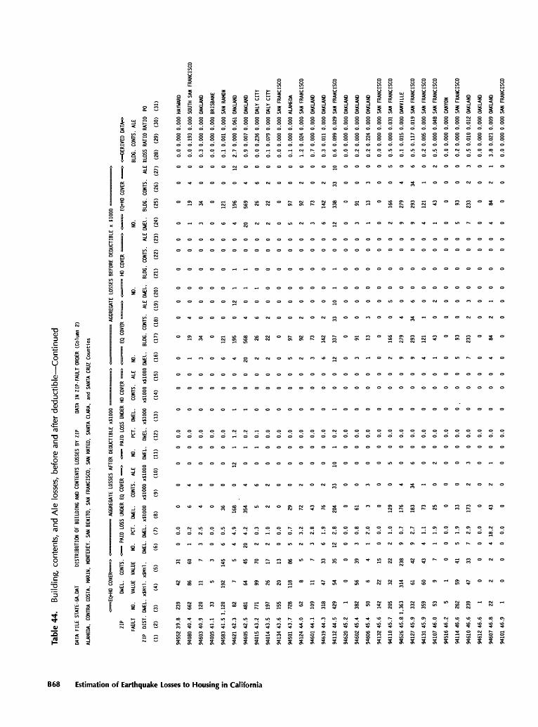
Tabl

e 44

. B

uild

ing,

con

tent

s, a

nd A

le l

osse

s, b

efor

e an

d af

ter

deduct

ible

Contin

ued

8.

5* of

Earthq g 5" o $ o X o i. 3 era 5' £ f 3 5*

ALAM

EDA.

CO

NTRA

CO

STA,

M

ARIN

, M

ONT

EREY

.

ZIP

FAU

LT

ZIP

D

IST

.

(1)

(2)

9455

2 3

9.8

9408

0 4

0.4

9460

3 4

0.9

9400

5 4

1.1

9458

3 4

1.5

9462

1 4

2.3

9460

5 4

2.5

9401

5 4

3.2

9401

4 4

3.5

9413

4 4

3.6

9450

1 4

3.7

9412

4 4

4.0

9460

1 4

4.1

9461

9 4

4.3

9411

2 4

4.5

9462

0 4

5.2

9460

2 4

5.4

9460

6 4

5.4

9413

2 4

5.6

9411

0 4

5.7

9452

6 4

5.8

9412

7 4

5.9

9413

1 4

5.9

9410

7 4

6.0

9451

6 4

6.2

9411

4 4

6.6

9461

0 4

6.6

9461

2 4

6.6

9460

7 4

6.8

9410

1 4

6.9

NO.

rnu

\*U

Yt.

i\ "

-

DWEL

. CO

NTS.

<

VALU

E VA

LUE

DWEL

. x$

Mil.

x$

Mil.

(3) 239

662

120 33

1,12

0 82 481

771

197

155

728 62 109

318

429 1

382 50 142

205

1,36

3

332

359 53 5

262

239 1

22 1

(4) 42 86 11 5

192 7 64 99 26 20 118 8 11 47 54 0 56 6 22 32 314 61 60 9 1 59 47 0 2 0

(5) 31 60 7 3

145 5 45 70 17 13 86 5 7 33 35 0 39 4 15 22 238 42 43

7 0

41 33 0 2 0

SAN

BE

NIT

O,

SAN

FRAN

CIS

CO

. SA

N M

ATED

, SA

NTA

CLAR

A,

and

SANT

A CR

UZ

Countie

s

y=

P

AID

LO

SS

UNDE

R EQ

COV

ER »

=>

<

=

PA

ID

LOSS

UN

DER

HO C

OVE

R =

=>

NO.

PCT.

DW

EL.

CONT

S.

ALE

NO.

PCT.

DW

EL.

CONT

S.

ALE

DWEL

.

(6) 0 1 3 0 6 4 20 2 2 0 5 2 3 6 12 0 3 1 0 2 9 9 4 1 0 5 7 0 4 0

DWEL

.

(7)

0.0

0.2

2.5

0.0

0.5

4.9

4.2 0.3 1.0

0.0

0.7

3.2

2.8 1.9

2.8

0.0

0.8

2.0

0.0

1.0

0.7

2.7 1.1

1.9 0.0 1.9

2.9 0.0

18.2

0.0

x$10

00

(8)

0 6 4 0 36 168

354 5 2 0 29 72 43 76 204 0 61 3 0

129

176

183 73 25

0 33 173 0

43 0

«. .

NO.

x$10

00 x

$100

0 DW

EL.

DWEL

. x$

1000

x$

1000

x$1

000

DWEL

.

(9)

(10)

(11)

(12)

(13)

(14)

(1

5)

0 0

0 0.0

0

00

4 0

0 0.0

0

00

0 0

0 0.0

0

00

0 0

0 0.0

0

00

0 0

0 0.0

0

00

0 12

1

1.2

1

00

4 0

1 0

.2

1 0

0

6 0

1 0

.1

0 0

0

2 0

0 0.0

0

00

0 0

0 0.0

0

00

0 0

0 0.0

0

00

2 0

0 0

.0

0 00

0 0

0 0.0

0

00

2 0

0 0

.0

0 0

0

33

10

1 0.2

1

00

0 0

0 0.0

0

00

0 0

0 0.0

0

00

3 0

0 0

.0

0 0

0

0 0

0 0.0

0

00

0 5

0 0.0

0

00

4 0

0 0

.0

0 0

0

34

6 0

0.0

0

00

1 0

0 0.0

0

00

0 2

0 0

.0

0 0

0

0 0

0 0.0

0

00

0 0

0 0.0

0

, 0

0

2 3

0 0

.0

0 0

0

0 0

0 0.0

0

00

2 1

0 0.0

0

00

0 0

0 0

.0

0 0

0

(16)

0 1 3 0 6 4 20 2 2 0 5 2 3 6 12 0 3 1 0 2 9 9 4 1 0 5 7 0 4 0

EQ

COV

ER

> <

H

O CO

VER =

=>

<

-

EQ+H

O CO

VER

<

NO.

NO.

BLD

G.

(17) 0 19 34 0

121

195

568 26 22 0 97 92 73 142

337 0 91 13 0

166

279

293

121 43

0 93 233 0

84 0

CONT

S.

(18) 0 4 0 0 0 0 4 6 2 0 0 2 0 2 33 0 0 3 0 0 4 34 1 0 0 0 2 0 2 0

ALE

DWEL

.

(19)

0 0 0 0 0 12 0 0 0 0 0 0 0 0 10 0 0 0 0 5 0 6 0 2 0 0 3 0 1 0

(20) 0 0 0 0 0 1 1 1 0 0 0 0 0 0 1 0 0 0 0 0 0 0 0 0 0 0 0 0 0 0

BLD

G.

CONT

S.

(21)

(22)

0 0

0 0

0 0

0 0

0 0

1 0

1 0

0 0

0 0

0 0

0 0

0 0

0 0

0 0

1 0

0 0

0 0

0 0

0 0

0 0

0 0

0 0

0 0

0 0

0 0

0 0

0 0

0 0

0 0

0 0

ALE

(23)

0 0 0 0 0 0 0 0 0 0 0 0 0 0 0 0 0 0 0 0 0 0 0 0 0 0 0 0 0 0

DWEL

.

(24)

0 1 3 0 6 4 20 2 2 0 5 2 3 6 12 0 3 1 0 2 9 9 4 1 0 5 7 0 4 0

BLD

G.

(25) 0 19 34 0

121

196

569 26 22 0 97 92 73 142

338 0 91 13 0

166

279

293

121 43

0 93 233 0 84 0

CONT

S.

(26) 0 4 0 0 0 0 4 6 2 0 0 2 0 2 33 0 0 3 0 0 4 34 1 0 0 0 2 0 2 0

=>

<=

DE

RIV

ED

DA

TA=>

BLD

G.

CONT

S.

ALE

ALE

XLO

SS

RAT

IO R

ATIO

PO

(27) 0 0 0 0 0 12 0 0 0 0 0 0 0 0 10 0 0 0 0 5 0 6 0 2 0 0 3 0 1 0

(28)

(29)

(30)

(31)

0.0

0.

000

0.00

0 HA

YWAR

D

0.0

0.

193

0.00

0 SO

UTH

SAN

FRAN

CISC

O

0.3

0.

000

0.00

0 O

AKLA

ND

0.0

0.

000

0.00

0 BR

ISBA

NE

0.1

0.00

1 0.

000

SAN

RAM

ON

2.7

0.0

00 0

.061

O

AKLA

ND

0.9

0.

007

0.00

0 O

AKLA

ND

0.0

0.

236

0.00

0 DA

LY

CIT

Y

0.1

0.

079

0.00

0 DA

LY

CIT

Y

0.0

0.

000

0.00

0 SA

N FR

ANCI

SCO

0.1

0.00

0 0.

000

ALAM

EDA

1.2

0.

024

0.00

0 SA

N FR

ANC

ISC

O

0.7

0.

000

0.00

0 O

AKLA

ND

0.3

0.

011

0.00

0 O

AKLA

ND

0.6

0.

099

0.02

9 SA

N FR

ANCI

SCO

0.0

0.

000

0.00

0 O

AKLA

ND

0.2

0.

000

0.00

0 O

AKLA

ND

0.2

0.2

24 0

.000 O

AKLA

ND

0.0

0.

000

0.00

0 SA

N FR

ANCI

SCO

0.5

0.

000

0.03

1 SA

N FR

ANCI

SCO

0.1

0.01

5 0.

000

DAN

VILL

E

0.5

0.

117

0.01

9 SA

N FR

ANCI

SCO

0.2

0.

005

0.00

0 SA

N FR

ANCI

SCO

0.5

0.

000

0.04

8 SA

N FR

ANC

ISC

O

0.0

0.

000

0.00

0 CA

NYON

0.2

0.

000

0.00

0 SA

N FR

ANCI

SCO

0.5

0.

010

0.01

2 O

AKLA

ND

0.0

0.

000

0.00

0 O

AKLA

ND

3.8

0.

021

0.00

9 O

AKLA

ND

0.0

0.0

00 0

.000 S

AN F

RAN

CIS

CO

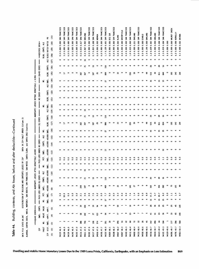
Dwelling and

Mob ile

Hom

e Mone if r- i o n 9 3- n eo o o a sr n Si. g -F m S> .O 1(v j. Lt 3 m o 1*

.

35*

O p- 8 t/

1 m 3* & o 3 CO

Tabl

e 44

. B

uild

ing,

con

tent

s, a

nd A

le l

osse

s, b

efor

e an

d af

ter

dedu

ctib

le C

ontm

uet

DATA

FIL

E ST

ATE-

6A.D

AT

DIS

TRIB

UTI

ON

OF

BUIL

DING

AND

CON

TENT

S LO

SSES

BY

ZIP

DA

TA I

N Z

IP-F

AULT

ORD

ER (

Col

umn

ALAM

EDA,

CO

NTRA

COS

TA,

MAR

IN,

MONT

EREY

, SA

N BE

NITO

. SA

N FR

ANCI

SCO,

SA

N M

ATED

, SA

NTA

CLAR

A,

and

SANT

A CR

UZ C

ount

ies

ZIP

FAUL

T

ZIP

D

IST.

(1)

(2)

9411

9 46

.9

9412

8 46

.9

9413

9 46

.9

9414

6 46

.9

9410

3 47

.0

9411

6 47

.2

9461

1 47

.4

9410

2 47

.6

9411

7 47

.6

9455

6 47

.6

9410

5 47

.7

9412

2 48

.0

9392

0 48

.1

9410

8 48

.2

9450

7 48

.2

9392

7 48

.3

9410

9 48

.3

9411

5 48

.4

9460

9 48

.4

9413

3 48

.6

9452

8 48

.6

9460

8 48

.6

9411

8 48

.7

9461

8 48

.7

9412

3 49

.2

9412

1 49

.3

9412

9 49

.6

9459

5 49

.7

9470

5 49

.7

9456

3 50

.3

DWEL

. CO

NTS.

<

= P

AID

LOSS

UND

ER E

Q CO

VER

==

>

<=

PAI

D L

OSS

UNDE

R HO

COV

ER =

>

NO.

VALU

E VA

LUE

NO.

PCT.

DW

EL.

CONT

S.

ALE

NO.

PCT.

DW

EL.

CONT

S.

ALE

DWEL

. x$

Mil.

x$

Mil.

DW

EL.

DWEL

. x$

1000

x$

1 000

x$

1000

DW

EL.

DWEL

. x$

1000

x$

1000

xJl

OO

O

(3)

(4)

(5)

(6)

(7)

(8)

(9)

(10)

(1

1)

(12)

(1

3)

(14)

(1

5)

1 2 1 1 8

388

700 3

106

574 1

351 18 3

290 16 22 68 72 22 26 45 142

286 66 184 1

177

286

580

0 1 0 0 1 58 142 1 27 123 0 54 5 1 77 1 9 23 8 7 7 5 41 51 23 36 0 33 65 140

0 0 0 0 1 39 100 0 19 94 0 36 3 0 59 1 7 16 6 5 5 3 28 36 16 25 0 25 45 105

0 1 0 0 0 8 4 0 8 1 0 27 0 0 1 0 0 5 1 0 0 4 16 2 15 15 0 2 4 4

0.0

50.0

0.0

0.0

0.0

2.1

0.6

0.0

7.5

0.2

0.0

7.7

0.0

0.0

0.3

0.0

0.0

7.4

1.4

0.0

0.0

8.9

11.3 0.7

22.7

8.2

0.0

1.1

1.4

0.7

0 7 0 0 0

249

197 0 66 8 0

469 0 0 23 0 0

145 27 0 0 8

301 9

454

282 0 75 101 99

0 0 0 0 0 5 21 0 10 0 0

116 0 0 0 0 0 4 0 0 0 9 20 0 29 16 0 0 0 0

0 0 0 0 0 6 16 0 1 0 0 1 0 0 0 0 0 0 9 0 0 0 0 0 5 3 0 0 0 3

0 0 0 0 0 0 0 0 0 0 0 2 0 0 0 0 0 0 0 0 0 0 0 0 1 2 0 0 0 0

0.0

0.0

0.0

0.0

0.0

0.0

0.0

0.0

0.0

0.0

0.0

0.6

0.0

0.0

0.0

0.0

0.0

0.0

0.0

0.0

0.0

0.0

0.0

0.0

1.5

1.1

0.0

0.0

0.0

0.0

0 0 0 0 0 0 0 0 0 0 0 13 0 0 0 0 0 0 0 0 0 0 0 0 0 10 0 0 0 0

0 0 0 0 0 0 0 0 0 0 0 0 0 0 0 0 0 0 0 0 0 0 0 0 0 0 0 0 0 0

0 0 0 0 0 0 0 0 0 0 0 0 0 0 0 0 0 0 0 0 0 0 0 0 0 0 0 0 0 0

<lllll

III""*

NO.

DWEL

.

(16) 0 1 0 0 0 8 4 0 8 1 0 27 0 0 1 0 0 5 1 0 0 4 16 2 15 15 0 2 4 4

1 2) »

Ap

rorp

AT

r i n

cccc

ocr

noc

- E

Q CO

VER

>

;

HO C

OVER

=

>

<=

= E

O+HO

COV

ER =

-> <

=DER

IVED

DAT

A=>

NO.

NO.

BLDG

. CO

NTS.

AL

E

BLDG

. CO

NTS.

AL

E DW

EL.

BLDG

. CO

NTS.

AL

E DW

EL.

BLDG

. CO

NTS.

AL

E *L

OSS

RAT

IO R

ATIO

PO

(17)

(1

8)

(19)

(2

0)

(21)

(2

2)

(23)

(2

4)

(25)

(2

6)

(27)

(2

8)

(29)

(3

0)

(31)

0 17 0 0 0

362

307 0

187 25 0

886 0 0 33 0 0

235 39 0 0 48 516 30 811

834 0

105

142

144

0 0 0 0 0 5 21 0 10 0 0

116 0 0 0 0 0 4 0 0 0 9 20 0 29 16 0 0 0 0

0 0 0 0 0 6 16 0 1 0 0 1 0 0 0 0 0 0 9 0 0 0 0 0 5 3 0 0 0 3

0 0 0 0 0 0 0 0 0 0 0 2 0 0 0 0 0 0 0 0 0 0 0 0 1 2 0 0 0 0

0 0 0 0 0 0 0 0 0 0 0 13 0 0 0 0 0 0 0 0 0 0 0 0 0 10 0 0 0 0

0 0 0 0 0 0 0 0 0 0 0 0 0 0 0 0 0 0 0 0 0 0 0 0 0 0 0 0 0 0

0 0 0 0 0 0 0 0 0 0 0 0 0 0 0 0 0 0 0 0 0 0 0 0 0 0 0 0 0 0

0 1 0 0 0 8 4 0 8 1 0 27 0 0 1 0 0 5 1 0 0 4 16 2 15 15 0 2 4 4

0 17 0 0 0

362

307 0

187 25 0

899 0 0 33 0 0

235 39 0 0 48 516 30 811

844 0

105

142

144

0 0 0 0 0 5 21 0 10 0 0

116 0 0 0 0 0 4 0 0 0 9 20 0 29 16 0 0 0 0

0 0 0 0 0 6 16 0 1 0 0 1 0 0 0 0 0 0 9 0 0 0 0 0 5 3 0 0 0 3

0.0

0.00

0 0.

000

SAN

FRAN

CISC

O

3.2

0.00

0 0.

000

SAN

FRAN

CISC

O

0.0

0.00

0 0.

000

SAN

FRAN

CISC

O

0.0

0.00

0 0.

000

SAN

FRAN

CISC

O

0.0

0.00

0 0.

000

SAN

FRAN

CISC

O

0.6

0.01

5 0.

017

SAN

FRAN

CISC

O

0.2

0.06

7 0.

052

OAKL

AND

0.0

0.00

0 0.

000

SAN

FRAN

CISC

O

0.7

0.05

3 0.

008

SAN

FRAN

CISC

O

0.0

0.00

0 0.

000

MORA

GA

0.0

0.00

0 0.

000

SAN

FRAN

CISC

O

1.7

0.12

9 0.

001

SAN

FRAN

CISC

O

0.0

0.00

0 0.

000

BIG

SUR

0.0

0.00

0 0.

000

SAN

FRAN

CISC

O

0.0

0.00

0 0.

000

ALAM

O

0.0

0.00

0 0.

000

GRE

ENFI

ELD

0.0

0.00

0 0.

000

SAN

FRAN

CISC

O

1.0

0.01

5 0.

000

SAN

FRAN

CISC

O

0.5

0.00

0 0.

231

OAKL

AND

0.0

0.00

0 0.

000

SAN

FRAN

CISC

O

0.0

0.00

0 0.

000

DIAB

LO

1.0

0.19

6 0.

000

OAKL

AND

1.2

0.03

9 0.

001

SAN

FRAN

CISC

O

0.1

0.00

0 0.

000

OAKL

AND

3.6

0.03

5 0.

006

SAN

FRAN

CISC

O

2.3

0.01

9 0.

004

SAN

FRAN

CISC

O

0.0

0.00

0 0.

000

0.3

0.00

0 0.

000

WAL

NUT

CREE

K

0.2

0.00

0 0.

000

BERK

ELEY

0.1

0.00

0 0.

021

ORI

NOA

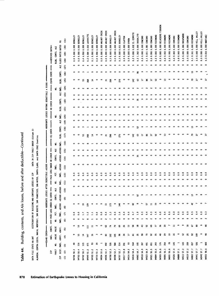
Tabl

e 44

. B

uild

ing,

con

tent

s, a

nd A

le l

osse

s, b

efor

e an

d af

ter

de

du

ctib

le C

on

tinu

ed

DATA

FILE

STATE-6A.DAT

DIST

RIBU

TION

OF

BUIL

DING

AND

CONTENTS

LOSSES B

Y ZIP

DATA

IN ZI

P-FA

ULT

ORDE

R (C

olum

n 2)

ALAMEDA. CONTRA C

OSTA

. MA

RIN,

MONTEREY,

SAN

BENI

TO.

SAN

FRANCISCO, SAN

MATE

D. SANTA

CLAR

A, an

d SA

NTA

CRUZ C

ounties

|- jf

Earthquake 1 i s- X o 5 cf 5* n a> f 3 5*

ZIP

FAULT

ZIP

DIST

.

(1)

(2)

94704

50.3

94703

50.4

94702

50.7

94549

51.2

94709

51.2

94710

51.3

94594

51.6

94596

51.7

9470

8 52

.3

9459

8 52.7

94707

52.7

94517

53.8

94514

54.2

94530

54.4

94965

54.7

94518

54.9

94523

54.9

94521

55.5

94804

55.5

94920

55.8

94805

56.3

9480

1 56

.8

94520

57.0

94808

57.1

94513

57.2

94519

57.2

94803

57.7

9494

1 57.7

94942

57.7

94553

58.0

DWEL

. CONTS. <-= P

AID

LOSS U

NDER

EQ CO

VER =>

< P

AID

LOSS U

NDER H

O COVER =>

NO.

VALU

E VALUE

NO.

PCT.

DW

EL.

CONT

S.

ALE

NO.

PCT.

DWEL.

CONT

S.

ALE

DWEL.

x$Mi

l. x$M11.

DWEL

. DWEL.

x$ 10

00

x$1000 x

$100

0 DW

EL.

DWEL.

x$1000 x$

1000

x$1

000

(3)

(4)

(5)

(6)

(7)

(8)

(9)

(10)

(1

1)

(12)

(1

3)

(14)

(1

5)

48 116

115

671 93 20 1

492

526

584

514

201 93 554

105

397

491

651

243

176

254 78 145 1

103

209

657

526 1

660

9 15 14 147 16 3 0 83 102

105 98 34 17 81 25 58 70 92 25 48 29 10 16 0 12 25 92 109 0 90

6 10 9

111 11 2 0 62 74 79 69 26 13 58 18 43 52 68 17 36 20 7 11 0 9 18 67 80 0 66

0 0 2 8 1 0 0 2 7 0 8 0 0 4 2 1 2 2 4 0 1 0 0 0 0 0 3 2 0 2

0.0

0.0

1.7

1.2

1.1

0.0

0.0

0.4

1.3

0.0

1.6

0.0

0.0

0.7

1.9

0.3

0.4

0.3

1.6

0.0

0.4

0.0

0.0

0.0

0.0

0.0

0.5

0.4

0.0

0.3

0 0 33 129 4 0 0 11 173 0

146 0 0 82 8 7 57 11 10 0 3 0 0 0 0 0 42 7 0 7

0 0 3 1 0 0 0 0 0 0 0 0 0 1 52 0 1 0 0 0 1 0 0 0 0 0 13 0 0 1

0 0 0 4 0 0 0 0 2 0 3 0 0 5 0 0 7 0 0 0 0 0 0 0 0 0 0 0 0 0

0 0 0 0 0 0 0 0 0 0 0 0 0 0 1 0 0 0 0 0 0 0 0 0 0 0 0 0 0 0

0.0

0.0

0.0

0.0

0.0

0.0

0.0

0.0

0.0

0.0

0.0

0.0

0.0

0.0

1.0

0.0

0.0

0.0

0.0

0.0

0.0

0.0

0.0

0.0

0.0

0.0

0.0

0.0

0.0

0.0

0 0 0 0 0 0 0 0 0 0 0 0 0 0 0 0 0 0 0 0 0 0 0 0 0 0 0 0 0 0

0 0 0 0 0 0 0 0 0 0 0 0 0 0 35 0 0 0 0 0 0 0 0 0 0 0 0 0 0 0

0 0 0 0 0 0 0 0 0 0 0 0 0 0 0 0 0 0 0 0 0 0 0 0 0 0 0 0 0 0

<< II NO.

DWEL

.

(16) 0 0 2 8 1 0 0 2 7 0 8 0 0 4 2 1 2 2 4 0 1 0 0 0 0 0 3 2 0 2

- E

Q COVER ==> < =» H

O COVER

> «s E

O+HO C

OVER

==->

<=OERIVED

DATA=>

NO.

NO.

BLDG

. CO

NTS.

AL

E

BLDG.

CONT

S.

ALE

DWEL

. BL

DG.

CONTS.

ALE

DWEL.

BLDG.

CONTS.

ALE

*LOS

S RATIO

RATI

O PO

(17)

(1

8)

(19)

(2

0)

(21)

(2

2)

(23)

(2

4)

(25)

(2

6)

(27)

(2

8)

(29)

(3

0)

(31)

0 0 53 268 14 0 0 31 298 0

270 0 0

142 63 17 86 37 52 0 13 0 0 0 0 0 79 27 0 37

0 0 3 1 0 0 0 0 0 0 0 0 0 1 52 0 1 0 0 0 1 0 0 0 0 0 13 0 0 1

0 0 0 4 0 0 0 0 2 0 3 0 0 5 0 0 7 0 0 0 0 0 0 0 0 0 0 0 0 0

0 0 0 0 0 0 0 0 0 0 0 0 0 0 0 0 0 0 0 0 0 0 0 0 0 0 0 0 0 0

0 0 0 0 0 0 0 0 0 0 0 0 0 0 0 0 0 0 0 0 0 0 0 0 0 0 0 0 0 0

0 0 0 0 0 0 0 0 0 0 0 0 0 0 35 0 0 0 0 0 0 0 0 0 0 0 0 0 0 0

0 0 0 0 0 0 0 0 0 0 0 0 0 0 0 0 0 0 0 0 0 0 0 0 0 0 0 0 0 0

0 0 2 8 1 0 0 2 7 0 8 0 0 4 2 1 2 2 4 0 1 0 0 0 0 0 3 2 0 2

0 0 53 268 14 0 0 31 298 0

270 0 0

142 63 17 86 37 52 0 13 0 0 0 0 0 79 27 0 37

0 0 3 1 0 0 0 0 0 0 0 0 0 1 86 0 1 0 0 0 1 0 0 0 0 0 13 0 0

, 1

0 0 0 4 0 0 0 0 2 0 3 0 0 5 0 0 7 0 0 0 0 0 0 0 0 0 0 0 0 0

0.0

0.000

0.000

BERK

ELEY

0.0

0.00

0 0.000

BERK

ELEY

0.4

0.059

0.000

BERK

ELEY

0.2

0.004

0.016

LAFA

YETT

E

0.1

0.000

0.000

BERK

ELEY

0.0

0.000

0.000

BERK

ELEY

0.0

0.000

0.000

WALN

UT CREEK

0.0

0.000

0.000

WALN

UT C

REEK

0.3

0.000

0.006

BERK

ELEY

0.0

0.000

0.000

WALN

UT CRE

EK

0.3

0.00

0 0.011

BERK

ELEY

0.0

0.000

0.000

CLAY

TON

0.0

0.00

0 0.000

BYRON

0.2

0.006

0.032

EL C

ERRI

TO

0.2

1.362

0.000

SAUS

ALIT

O

0.0

0.000

0.000

CONC

ORD

0.1

0.011

0.081

CONC

ORD

0.0

0.00

0 0.

000 CO

NCOR

D

0.2

0.000

0.000

RICH

MOND

0.0

0.000

0.000

BELV

EDER

E -TIBURON

0.0

0.053

0.000

RICH

MOND

0.0

0.000

0.000

RICH

MOND

0.0

0.000

0.000

CONC

ORD

0.0

0.00

0 0.000

RICH

MOND

0.0

0.000

0.00

0 BR

ENTW

OOD

0.0

0.000

0.000

CONC

ORD

0.1

0.161

0.000

RICH

MOND

0.0

0.000

0.000

MILL

VALLEY

o.o

o.ooo

o.ooo

MILL'.

VALLEY

0.6

0.033

0.000

MART

INEZ

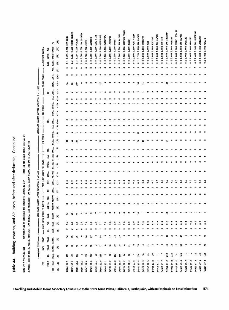
Tabl

e 44

. B

uild

ing,

con

tent

s, a

nd A

le l

osse

s, b

efor

e an

d af

ter

de

du

ctib

le C

on

tinu

ed

OQ

W a. o

DATA F

ILE

STAT

E-6A

.DAT

DI

STRI

BUTI

ON OF

BUIL

DING

AND

CON

TENT

S LO

SSES

BY

ZIP

DATA

IN ZI

P-FA

ULT ORDER

(Column

Z)

ALAMEDA. CO

NTRA

COS

TA.

HARI

N. MONTEREY.

SAN

BENI

TO.

SAN

FRAN

CISC

O. SAN

MATE

D. SA

NTA

CLAR

A, and

SANTA

CRUZ C

ounties

n _*

10

oo « n Si

.

f 3 JO w 5" i1 §-

ZIP

FAULT

ZIP

DIST

.

(1)

(2)

94806

5B.5

9492

5 58

.7

94564

59.2

94964

59.2

94547

59.4

94509

59.6

93930

59.7

94565

60.0

94548

60.1

94939

60.2

94561

60. B

9490

4 61.0

94970

61.2

94572

61.4

94569

62.0

94901

62.0

94525

62.5

94957

62.5

94924

62. B

94915

63.1

9451

0 63.2

9496

0 64.2

94930

64.8

94511

65.4

94903

65.4

9459

1 65.7

94590

66.4

94963

67. B

94973

67.8

94949

67.9

DWEL

. CONTS. < P

AID

LOSS U

NDER

EQ

COVER > < P

AID

LOSS U

NDER H

O COVER -=>

NO.

VALUE

VALU

E NO

. PC

T.

DWEL.

CONT

S.

ALE

NO.

PCT.

DW

EL.

CONT

S.

ALE

DWEL

. xS

Hil.

x$

H11.

DW

EL.

DWEL.

xllOOO

xllOOO x

$100

0 DWEL.

DWEL

. x$

100

0 xllOOO x

llOOO

(3) 476

136

383 1

252

727 29 698 2 B2 163

160 24 92 4

376 30 34 30 1 2

240

123 14 360 1 1 12 40 148

(4)

(5)

52 20 49 0 36 90 3 77 0 16 19 38 4 11 0 78 4 11 5 0 0 42 IB 2 56 0 0 2 6 29

36 15 36 0 26 67 2 56 0 12 14 29 3 8 0 59 3 B 4 0 0 31 13 1 42 0 0 2 5 22

(6) 2 2 6 0 0 0 0 2 0 0 0 0 0 0 0 3 1 0 0 0 0 1 0 0 0 0 0 0 0 0

(7)

0.4

1.5

1.6

0.0

0.0

0.0

0.0

0.3

0.0

0.0

0.0

0.0

0.0

0.0

0.0

O.B

3.3

0.0

0.0

0.0

0.0

0.4

0.0

0.0

0.0

0.0

0.0

0.0

0.0

0.0

(B)

(9)

(10)

(1

1)

14 29 46 0 0 0 0 2 0 0 0 0 0 0 0 14 1 0 0 0 0 13 0 0 0 0 0 0 0 0

B 0 0 0 0 0 0 0 0 0 0 0 0 0 0 10 0 0 0 0 0 0 0 0 0 0 0 0 0 0

0 0 0 0 0 0 0 0 0 0 0 0 0 0 0 0 0 0 0 0 0 0 0 0 0 0 0 0 0 0

0 0 0 0 0 0 0 0 0 0 0 0 0 0 0 0 0 0 0 0 0 0 0 0 0 0 0 0 0 0

(12)

(1

3)

(14)

0.0

0.0

0.0

0.0

0.0

0.0

0.0

0.0

0.0

0.0

0.0

0.0

0.0

0.0

0.0

0.0

0.0

0.0

0.0

0.0

0.0

0.0

0.0

0.0

0.0

0.0

0.0

0.0

0.0

0.0

0 0 0 0 0 0 0 0 0 0 0 0 0 0 0 0 0 0 0 0 0 0 0 0 0 0 0 0 0 0

0 0 0 0 0 0 0 0 0 0 0 0 0 0 0 0 0 0 0 0 0 0 0 0 0 0 0 0 0 0

(15) 0 0 0 0 0 0 0 0 0 0 0 0 0 0 0 0 0 0 0 0 0 0 0 0 0 0 0 0 0 0

<jmiLj]

NO.

DWEL

.

(16) 2 2 6 0 0 0 0 2 0 0 0 0 0 0 0 3 1 0 0 0 0 1 0 0 0 0 0 0 0 0

- E

Q CO

VER

> :

HO C

OVER

>

; EQ+HO CO

VER

NO.

NO.

BLD6

. CO

NTS.

AL

E DW

EL.

BLD6

. CO

NTS.

AL

E DW

EL.

BLDG

. CO

NTS.

(17) 34 56 109 0 0 0 0 22 0 0 0 0 0 0 0 54 11 0 0 0 0 24 0 0 0 0 0 0 0 0

(18)

(1

9) (2

0)

B 0 0 0 0 0 0 0 0 0 0 0 0 0 0 10 0 0 0 0 0 0 0 0 0 0 0 0 0 0

0 0 0 0 0 0 0 0 0 0 0 0 0 0 0 0 0 0 0 0 0 0 0 0 0 0 0 0 0 0

0 0 0 0 0 0 0 0 0 0 0 0 0 0 0 0 0 0 0 0 0 0 0 0 0 0 0 0 0 0

(21) 0 0 0 0 0 0 0 0 0 0 0 0 0 0 0 0 0 0 0 0 0 0 0 0 0 0 0 0 0 0

(22) 0 0 0 0 0 0 0 0 0 0 0 0 0 0 0 0 0 0 0 0 0 0 0 0 0 0 0 0 0 0

(23) 0 0 0 0 0 0 0 0 0 0 0 0 0 0 0 0 0 0 0 0 0 0 0 0 0 0 0 0 0 0

(24) 2 2 6 0 0 0 0 2 0 0 0 0 0 0 0 3 1 0 0 0 0 1 0 0 0 0 0 0 0 0

(25) 34 56 109 0 0 0 0 22 0 0 0 0 0 0 0 54 11 0 0 0 0 24 0 0 0 0 0 0 0 0

> <=DERIVED

DATA

->

BLDG

. CONTS. AL

E

ALE

*LOSS

RATI

O RA

TIO

PO

(26)

(2

7)

8 0 0 0 0 0 0 0 0 0 0 0 0 0 0 10 0 0 0 0 0 0 0 0 0 0 0 0 0 0

0 0 0 0 0 0 0 0 0 0 0 0 0 0 0 0 0 0 0 0 0 0 0 0 0 0 0 0 0 0

(2B)

(2

9)

(30)

(3

1)

0.1

0.235

0.000

RICH

MOND

0.3

0.00

7 0.000

CORT

E MA

DERA

0.2 0.

004

0.000

PINO

LE

0.0

0.000

0.000

SAN QU

ENTI

N

0.0

0.000

0.000

RODEO

0.0

0.000

0.000

ANTI

OCH

0.0

0.000

0.000

KING

CIT

Y

0.0

0.000

0.000

PITT

SBUR

G

0.0

0.000

0.000

KNIG

HTSE

N

0.0

0.000

0.000

LARK

SPUR

0.0

0.000

0.000

OAKL

EY

0.0

0.000

0.000

SAN RA

FAEL

0.0

0.000

0.000

STIN

SON

BEACH

0.0

0.000

0.000

RODEO

0.0

0.000

0.000

PORT

COS

TA

0.1

0.178

0.000

SAN

RAFA

EL

0.3

0.000

0.000

CROC

KETT

0.0

0.000

0.000

ROSS

0.0

0.000

0.000

BOLI

NAS

0.0

0.000

0.000

SAN

RAFA

EL

0.0

0.000

0.000

BENI

CIA

0.1

0.000

0.000

SAN AN

SELM

O

0.0

0.000

0.000

FAIR

FAX

0.0

0.000

0.000

BETHEL ISLAND

0.0

0.000

0.000

SAN

RAFA

EL

0.0

0.000

0.000

VALL

EJO

0.0

0.000

0.000

VALL

EJD

0.0

0.000

0.000

SAN

GERO

NIMO

0.0

0.000

0.000

WOOD

ACRE

0.0

0.000

0.000

NOVATO

B72

Estimation

ol m V f

£ 5" fD 8 n (A s I § . OQ 3* n 2L S o 3 55°

Tabl

e 44

. B

uild

ing,

con

tent

s, a

nd A

le l

osse

s, b

efor

e an

d af

ter

dedu

ctib

le C

ontin

ued

DATA

FI

LE

STA

TE-6

A.D

AT

DIS

TRIB

UTI

ON

OF

BU

ILD

ING

AN

D CO

NTEN

TS

LOSS

ES B

Y Z

IP

DATA

IN

ZIP

-FA

ULT

ORD

ER

(Col

umn

2)

ALAM

EDA,

CO

NTRA

CO

STA,

M

ARIN

, M

ONT

EREY

, SA

N BE

NIT

O.

SAN

FRAN

CIS

CO

, SA

N M

ATED

. SA

NTA

CLA

RA,

an

d SA

NTA

CRUZ

C

ountie

s

ZIP

FAU

LT

ZIP

D

IST

.

(1)

(2)

945B

9 6

9.2

9493

3 6

9.2

9493

8 6

9.4

9494

7 7

1.3

9495

0 7

1.7

9494

5 72

.1

9494

6 73

.0

9453

3 76

.6

9495

6 76

.6

9453

5 7

6.7

9393

2 78

.1

9493

7 7

8.3

9495

2 B

1.9

9494

0 8

2.1

9492

8 B

9.2

9492

9 90

.1

> c.

VJT

RU

i/ v

/ Y 1

. 1\ --

*

DU

EL.

CONT

S.

<

NO.

VALU

E VA

LUE

DU

EL.

xSH

il.

xSH

il.

(3) 1 9 11 371 2

255 8 1 15 1 2 33 3 7 1 8

(4) 0 1 2 60

0

44

3 0 2 0 0 5 0 1 0 1

(5)

0 1 1

45 0 34 2 0 2 0 0 3 0 1 0 1

3 P

AID

LO

SS

UNDE

R EQ

COV

ER -

=>

<

PA

ID

LOSS

UN

DER

HO C

OVER

=>

NO.

PCT.

D

UEL

. CO

NTS.

AL

E NO

. PC

T.

DU

EL.

CONT

S.

ALE

DU

EL.

DU

EL.

xllO

OO

xJ

lOO

O

xllO

OO

D

UEL

. D

UEL

. xl

lOO

O

xllO

OO

x$1

000

(6) 0 0 0 0 0 2 0 0 0 0 0 0 0 0 0 0

(7)

0.0

0.0

0.0 0.0

0.0

O.B

0.0 0.0

0.0 0.0 0.0

0.0

0.0

0.0 0.0

0.0

(8)

0 0 0 0 0 3' 0 0 0 0 0 0 0 0 0 0

(9)

(10)

(11)

(12)

0 0

0 0

.0

0 0

0 0

.0

0 0

0 0.0

0 0

0 0.0

0 0

0 0.0

0 0

0 0.0

0 0

0 0

.0

0 0

0 0.0

0 0

0 0.0

0 0

0 0.0

0 0

0 0.0

0 0

0 0.0

0 0

0 0.0

0 0

0 0.0

0 0

0 0.0

0 0

0 0.0

(13)

(14)

0 0

0 0

0 0

0 0

0 0

0 0

0 0

0 0

0 0

0 0

0 0

0 0

0 0

0 0

0 0

0 0

(15) 0 0 0 0 0 0 0 0 0 0 0 0 0 0 0 0

<Ju

m»

»u

NO.

DU

EL.

(16)

0 0 0 0 0 2 0 0 0 0 0 0 0 0 0 0

» EQ

COV

ER =

=>

:

HO C

OVER

«=

> <

~

EO+

HO C

OVER

NO.

NO.

BLD

G.

CONT

S.

ALE

DU

EL.

BLD

G.

CONT

S.

ALE

DU

EL.

BLD

G.

CONT

S.

(17) 0 0 0 0 0

39 0 0 0 0 0 0 0 0 0 0

(18) 0 0 0 0 0 0 0 0 0 0 0 0 0 0 0 0

(19) 0 0 0 0 0 0 0 0 0 0 0 0 0 0 0 0

(20) 0 0 0 0 0 0 0 0 0 0 0 0 0 0 0 0

(21) 0 0 0 0 0 0 0 0 0 0 0 0 0 0 0 0

(22) 0 0 0 0 0 0 0 0 0 0 0 0 0 0 0 0

(23)

(24)

0 0

0 0

0 0

0 0

0 0

0 2

0 0

0 0

0 0

0 0

0 0

0 0

0 0

0 0

0 0

0 0

(25) 0 0 0 0 0 39 0 0 0 0 0 0 0 0 0 0

(26) 0 0 0 0 0 0 0 0 0 0 0 0 0 0 0 0

==

>

<=D

ER

IVE

D

DAT

A=>

BLD

G.

CONT

S.

ALE

ALE

*LO

SS

RAT

IO R

ATIO

PO

(27) 0 0 0 0 0 0 0 0 0 0 0 0 0 0 0 0

(28)

(2

9)

(30)

(3

1)

0.0

0.

000

0.00

0 VA

LLEJ

O

0.0

0.

000

0.00

0 FO

REST

KNO

LLS

0.0

0.

000

0.00

0 LA

GU

NIT

AS

0.0

0.

000

0.00

0 NO

VATO

0.0

0.

000

0.00

0 O

LEM

A

0.1

0.00

0 0.

000

NOVA

TO

0.0

0.

000

0.00

0 N

ICA

SIO

0.0

0.0

00

0.00

0 FA

IRFI

ELO

0.0

0.

000

0.00

0 PO

INT

REYE

S ST

ATIO

N

0.0

0.

000

0.00

0 FA

IRFI

ELO

0.0

0.

000

0.00

0 LO

CKW

OOO

0.0

0.0

00

0.00

0 IN

VERN

ESS

0.0

0.

000

0.00

0 PE

TALU

MA

0.0

0.

000

0.00

0 M

ARSH

ALL

0.0

0.

000

0.00

0 C

OTA

TI

0.0

0.

000

0.00

0 D

ILLO

N B

EACH

84,4

23

13,5

20

9.9B7

2.784

63,9

85

14,885

5.159

245

2.391

467

115

2,78

4 11

4,86

4 14.885 5

,159

230

1,94

1 46

7 11

5 3.014

116.

805

15.352 5

,275

NOTE

S:

Colu

mn 7

: PC

T. DU

EL.

- Column 6

div

ided

by

colu

mn 3

. in

*.

Colu

mn 1

2:

PCT.

DU

EL.

- Co

lunn

11

divided

by c

olumn

3 in

*.

Colu

mn 2

8:

BLDG.

XLOSS - Average

buil

ding

loss

as a

* o

f insured

valu

e, be

fore

ded

ucti

ble.

Column 1

7 di

vide

d by

col

umn

4. in

X.

Colu

mn 2

9:

CONT

S. RATIO *

(Aggregate c

ontents

loss [c

olumn

26])

divi

ded

by (

Aggregate

buil

ding

los

s before d

eductible

[col

umn

25]).

Colu

mn 3

0:

ALE

RATI

O -

(Aggregate A

LE l

oss

[has n

o de

duct

ible

-

co

lumn

27]

) divided

by

(Aggregate b

uilding

loss b

efor

e deductible [

colu

mn 2

5]).