A DYNAMIC CHARACTERIZATION OF EFFICIENCY

Spiro E. Stefanou*

Professor of Agricultural Economics Pennsylvania State University (USA)

Revised October 2006

Abstract: The definition and measurement of dynamic economic performance has been addressed obliquely in the literature with the notions of scope economies and capacity utilization measures, but little work has focused on develop the static theory analogs of efficiency measures into the dynamic context. This paper is an attempt to identify some of the conceptual and methodological issues to be addressed. A model allowing for dynamic production decisions in the face of inefficiency is presented to illustrate some of the issues and the extensions necessary to identify truly dynamic performance measures. * Spiro E. Stefanou acknowledges the support of the Marie Curie Transfer of Knowledge Fellowship of the European Community's Sixth Framework Program at the Department of Economics at the University of Crete under contract number MTKD-CT-014288 during Spring 2006.

1

A Dynamic Characterization of Efficiency

I. INTRODUCTION

The issue of dynamic efficiency is an important component in assessing capital

accumulation patterns and growth. Early characterizations of efficiency over time focus

on how the capital stock relates to the Golden Rule level (Phelps, 1961; Diamond, 1965).

Others focus on how the presence of dynamic efficiency facilitates intergenerational

transfer of assets (Weil, 1987) and can eliminate the prospect of speculative bubbles

(Tirole, 1985). Abel et al. (1989) investigate if capital accumulation levels of OECD

economies operate above or below Golden Rule levels. Most of these studies have a

distinctly macroeconomic policy orientation. However, the extent of inefficient behavior

in the management of dynamic assets at the firm level has not been clearly characterized

or modeled.

The determination of efficient behavior discussed here is temporal in nature by

describing the degree of efficiency of the firm at a particular point of its adjustment path.

The firm's optimal adjustment path over time and the steady-state may vary with

temporal efficiency. This paper initiates a discussion of conceptual and methodological

issues revolving around the measurement of economic performance when firm make

decisions linked over time. A model allowing for dynamic production decisions in the

face of inefficiency is presented to illustrate some of the issues and the extensions

necessary to identify truly dynamic performance measures.

2

II. CONCEPTUAL ISSUES

When addressing the dynamic efficiency we need to distinguish between a) tracking

efficiency over time (which involves modeling exogenous versus endogenous forces and

the impact of covariates/environmental variables on econ performance), and b)

persistence which involves identifying the contributions of structural (deterministic)

sources and the stochastic sources. The sources of economic dynamics are:

• economic forces (for example, adjustment cost and financial constraint models),

• technological characteristics (for example, physical/biological nature of

production, and vintage investment/stock nonconvexities like we see with lumpy

investment), and

• cognitive capacity.

To date, our models do not separate our these forces, and thus, can confound the results

reported in the literature.

The economic forces can relate largely to adjustment processes which has been

classically presented in the literature as a dichotomy between the short and long runs.

The distinction between the short and long run becomes a prime consideration in

determining the appropriate time scale of economic decision making strategies. These

strategies focus on the choice of production factors assumed to be fixed when factor

allocation decisions are to be made. All economic activity occurs in the short-run to the

extent a factor (or factors) of production are taken as fixed. The long run refers to the

firm planning ahead to select a future short-run production situation. The problem with

the classical description of the short- and long-run is that the story of the envelope curve

is not entirely consistent with the story motivating the distinction between the short and

3

long run.1 The long run consists of a range of possible short run situations available to

the firm. As such, the firm always operates in the short run but plans for the long run. A

more complete description of producer behavior in the long-run theory of cost

concentrates on the planning problem involving the minimization of the discounted

stream of costs. Such a characterization focuses on long-run costs as a stock rather than

a flow concept.

The classical approach characterizes both short- and long-run cost functions as

flows. The long-run is merely the case where the fixed factor is now variable --

presumably because the time span under consideration is now long enough to view the

problem as a short-run planning problem. This could entail describing the short-run to

last 5 or 10 years given capital adjustment rates estimated in the empirical literature.

Viner’s (1931) idea of some factors being "freely adjusted" while others are "necessarily

fixed" is sufficiently vague to allow long-run costs to be considered a flow. Freely

adjusted implies that altering the input levels of these factors does not impose a penalty

on the firm other than a constant acquisition cost.

The application of non-freely adjusted inputs presumably occurs because some

additional costs must be absorbed by the firm beyond the acquisition cost. The

introduction of adjustment costs can capture this phenomenon. Some factors are

considered "fixed" in the short run, not because the operator is physically prevented from

removing or introducing more of the factor, but because the economic environment

places a high cost on adjusting the factor level. For example, it may be more profitable

1 Alchian (1959) and De Alessi (1967) recharacterize long-run costs as a discounted flow of costs that involve a sequence of production targets as represented by the volume of production over the time horizon. Stefanou (1989) recasts these formulations into a dynamic adjustment framework to create long- and short-run value functions.

4

at the margin to under or over utilize a given set of quasi-fixed factors rather than renting

the services of those factors (external adjustment costs). In addition, additional costs

may arise from the adjustment in the technical relationships (internal adjustment costs).

Temporal Efficiency and the Steady-State

The adjustment cost hypothesis states current additions to the stock of capital are

output decreasing at the time of investment but output increasing in the future by

increasing the future stock of capital. Thus, the firm's current investment decisions

involve a trade-off between instantaneous cost and the gains arising from future

production possibilities. The firm's optimal adjustment path over time and the steady-

state are likely to vary with the degree of temporal efficiency. Temporal efficiency is a

flow notion of dynamic efficiency in that the firm's decisions are assumed to be made in

the short run with a view to the long run.

Characterizing Dynamic Efficiency: Functional or Function?

The notion of efficient allocation of variable and quasi-fixed inputs in the long

run can take on a criterion based on stock efficiency or temporal efficiency. The stock-,

or functional-based notion of efficiency focuses on a capital trajectory that is a decision

path where perfectly efficient decisions are made at each decision point over the time

horizon. This is the efficiency characterization implied by Diamond (1965), Abel et al.

(1989) and Thalmann (1996). Focusing on this definition of dynamic efficiency is

extremely restrictive and not reflective of how decisions are made. If decisions are

always made in the short run with a view to the long run, then efficiency is a temporal

issue and not a comparison of trajectories. The temporal notion is also conditioned on

5

past decisions but reflects dynamic linkages of past decisions to future prospects. The

temporal notion of allocative efficiency reflects the operator making the right current

decisions towards long-run equilibrium.

Both characterizations of dynamic efficiency are conditional notions. Temporal

efficiency is a conditional notion in that current decisions are efficient given all past

(efficient or inefficient) investment decisions. A stock-based efficiency measure is also

conditional since the decision trajectory from, say, to to T is efficient given all (efficient

or inefficient) investment decisions previous to t=to. Assuming ko is not long-run

efficient due to unexpected price changes, for example, there is an inefficient trajectory

at some point previous to the initial period, to. However, if investment decisions are

made in the short run with a view to the long run, dynamic efficiency is a temporal

notion and does not involve an explicit comparison of trajectories. As a result, the stock

notion of dynamic efficiency does not reflect how investment decisions are made.

III. METHODOLGOICAL ISSUES

The approaches to measuring efficiency levels over time can be broadly classified as

those emanating from data-driven empirical approaches and those based on structural

models reflecting dynamic behavioral decisions permitting dynamic efficiency impacts.

The value of both approaches is substantial. The data driven approaches can provide

evidence and direction on where to look for inefficiency effects that the structural models

may assume away. Rarely are the structural models so all-encompassing as to nest all

sources of inefficiency. As the area of dynamic efficiency measurement gains greater

6

attention, the interplay emerges between theory-driven applications as well as

applications-drive theory.

There are two issues on the agenda of dynamics and efficiency measurement: 1)

what is the evidence of inefficiency behavior over time (e.g., do firms get better, stay the

same, get worse, get better then worse, …)?, and 2) what structural models of economic

decision making combined with the technological characteristics and cognitive capacity

can be developed to explain the patterns of efficiency behavior? An important question

of interest is if we must deal with the two issues simultaneously, or can we sequentially

address the two issues. Just measuring the efficiency level at each time point in isolation

will surely yield biased results. The production technology exhibits no technological

forces suggesting dynamic linkages over time. Since there is no behavioral resource

allocation model addressed, the choices of input use over time are taken exogenously.

In general, endogeneity issues are rarely addressed by decisions taken in an

earlier period influencing the distribution of the long-run efficiency level. Of course, it

depends on the factors z that one specifies, and this is a cautionary note that should be

sounded loudly. Surely, there are forcing factors and choices the decision maker can

execute to influence the long-run inefficiency level and these are the variables you would

include as covariates, z. A true unifying model should take into account the decision

processes and choices associated with choosing the levels of these forcing factors

influencing efficiency levels over time.

7

Dynamic versus Time-Varying Efficiency Measures:

Estimating the efficiency and productivity patterns over time is being revisited in

the literature as the data sets become richer. Recent studies in the analysis of

productivity changes find that there are serious problems in dealing with aggregate

measures of productivity. These studies indicate that the analysis of a sector or an

industry focusing only on aggregate productivity measures may be misleading,

presenting a simplistic explanation of the process. Dhrymes and Bartelsman (1998) and

Dhrymes (1991) find that two-digit industry wide productivity, and its growth over time,

may be reduced considerably upon addressing the four-digit industry composition of the

sample. Hence, a disaggregated analysis can provide a more detailed perspective of the

dynamics of total factor productivity (TFP) growth when compared with the aggregate

level analysis of TFP growth. Pakes and colleagues2 refine the effort by taking on

micro-level panel data sets to model the economic interactions leading to productivity

gains and some efficiency impacts. Exploiting the heterogeneity in the micro-level data

(plants or firms) leads to identifying the weakness of the theory developed with a macro

view of behavior. One example, is where the aggregate modeling suggests capital

adjustment is smooth process, the micro-level evidence strongly suggests the presence of

discontinuous (or lumpy) capital adjustment (Nilsen and Schiantarelli, 2003; Celikkol

and Stefanou, 2004). The presence of discontinuous capital changes can lead to much

different characterizations of efficiency since capital adjustment patterns may lead a firm

to appear to be overcapitalized in some periods and under capitalized in others.

2 Important references include Pakes and McGuire (1994), Ericson and Pakes (1995), Olley and Pakes (1996).

8

The modeling of time-varying efficiency historically appears as the specification

of time as a regressor which leads to the challenge of disentangling the two roles time

plays; namely, time as a proxy for technical change in the deterministic kernel of the

stochastic production frontier versus time as an indicator of technical efficiency change

in the composite error term. Historically, three popular specifications are present in the

literature, historically (Kumbhakar and Lovell, 2000):

• )(tuu iit γ= , where )(tγ is a parametric function of time and ui is a nonnegative

random variable (Kumbhakar, 1990, and Battese and Coelli, 1992);

• tiit uu γ= , where tγ are the time effects represented by time dummies and the ui

term can be either fixed or random producer-specific effects (Lee and Schmidt,

1993); and,

• 2321 ttu iiiit Ω+Ω+Ω= where the Ω ’s are producer-specific parameters

(Cornwell, Schmidt and Sickles, 1990).

A new generation of specifications is emerging that present themselves as dynamic

frontier approaches and have the goal of sorting out the long-run from the short-run

inefficiency levels. Ahn, Good and Sickles (2000) allow for the future arrival of

unexpected inefficiency sources by focusing on an autoregressive specification of

technical efficiency. This error structures intended to capture the sluggish adoption of

technological innovations that relate to long- and short-run dynamics rather than

incorporating a structural model of sluggish adoption. Tsionas (2006) allows for a

stochastic and unknown long-run efficiency level by taking a Bayesian perspective on

generating the short- and long-run efficiency distributions. The basic proposition is that

9

long-run inefficiency cannot be a deterministic limiting point when you start off with a

stochastic measure of short-run (or instantaneous) inefficiency.

Structural Modeling Approaches

The structural approaches to modeling dynamic efficiency involve both primal

and dual specifications. The earliest efforts go back to Shephard and Färe (1978) that

evolved into the Dynamic DEA models in Färe and Grosskopf (1996). This approach

takes on a network theory orientation addressing an intertemporal substitution among

inputs, outputs and intermediate outputs, and is particularly well-suited for multistage

production processes. By preserving the time-ordered sequence of decisions, the timing

of decisions permits the impact of technical inefficiency at one stage to be transmitted to

later stages. Sengupta (1995, 1997) take a primal perspective with the explicit

specification of a smooth adjustment cost function. Working with a linear-quadratic

specification, closed form solutions are presented at the cost of modeling additional

production flexibility. Nemoto and Giro (1999, 2003) take on a primal focus as well by

building a discrete time mathematical programming model as it related to dynamic

optimization theory. The fundamentals of this approach builds on Kleindorfer et al.

(1975) which constructs the discrete time variants of the optimal control theory’s

Pontryagin Principle.

Two new directions build on the dynamic production analysis frameworks found

in the same issue of the Journal of Productivity Analysis. Silva and Stefanou (2007)

develop a myriad of efficiency measures associated with the dynamic generalization of

the dual-based revealed preference approach to production analysis found in Silva and

10

Stefanou (2003). Vaneman and Triantis (2003) take on a system dynamics approach to

specify the axioms of dynamic production and then build off this foundation in Vaneman

and Triantis (2004) to measure a form of dynamic technical efficiency. By focusing on

system performance, they explicitly take into account the interactions and feedback

mechanisms that explain the causes of efficiency behavior, the dynamic nature of

production, and non-linear combinations of the input/output variables.

Another tack builds on the shadow value function approach pioneered by Toda

(1967) and Atkinson and Halvorson (1980), and then extended by Stefanou and Saxena

(1988), Atkinson and Cornwall (1994), and Kumbhakar (1997). In this context both

actual and behavioral value functions are constructed to capture how inefficiency leads to

deviations from optimal decisions. The next section develops a model to illustrate the

generalization of the shadow value function from an intertemporal perspective.3

IV. SHADOW VALUE FUNCTION MODEL

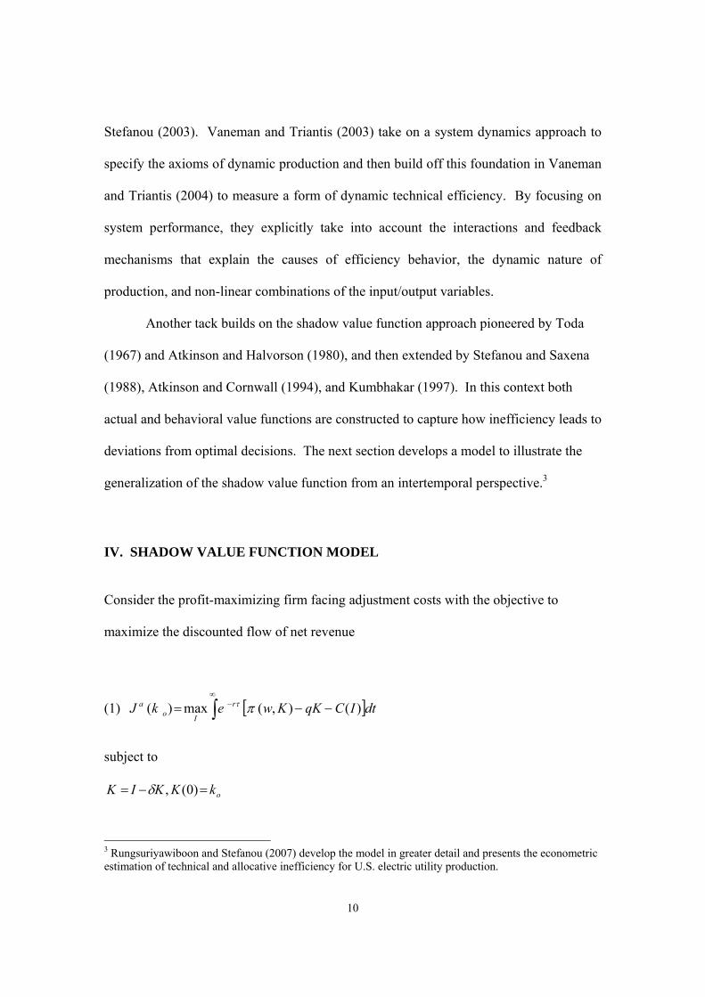
Consider the profit-maximizing firm facing adjustment costs with the objective to

maximize the discounted flow of net revenue

(1) [ ]dtICqKKwekJ r

Ioa )(),(max)( −−= −

∞

∫ πτ

subject to

okKKIK =−= )0(,δ

3 Rungsuriyawiboon and Stefanou (2007) develop the model in greater detail and presents the econometric estimation of technical and allocative inefficiency for U.S. electric utility production.

11

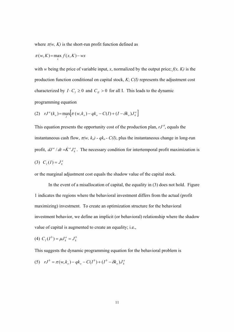
where π(w, K) is the short-run profit function defined as

wxKxfKwx

−= ),(max),(π

with w being the price of variable input, x, normalized by the output price; f(x, K) is the

production function conditional on capital stock, K; C(I) represents the adjustment cost

characterized by 0≥⋅ ICI and 0>IIC for all I. This leads to the dynamic

programming equation

(2) [ ]akoooIo

a JkIICqkkwkrJ )()(),(max)( δπ −+−−=

This equation presents the opportunity cost of the production plan, rJ a, equals the

instantaneous cash flow, π(w, ko) - qko - C(I), plus the instantaneous change in long-run

profit, ak

aa JKdtdJ &=/ . The necessary condition for intertemporal profit maximization is

(3) akI JIC =)(

or the marginal adjustment cost equals the shadow value of the capital stock.

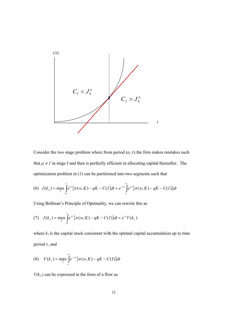
In the event of a misallocation of capital, the equality in (3) does not hold. Figure

1 indicates the regions where the behavioral investment differs from the actual (profit

maximizing) investment. To create an optimization structure for the behavioral

investment behavior, we define an implicit (or behavioral) relationship where the shadow

value of capital is augmented to create an equality; i.e.,

(4) bk

ak

bI JJIC == μ)(

This suggests the dynamic programming equation for the behavioral problem is

(5) ako

bboo

b JkIICqkkwrJ )()(),( δπ −+−−=

12

Consider the two stage problem where from period (o, τ) the firm makes mistakes such

that μ ≠ 1 in stage I and then is perfectly efficient in allocating capital thereafter. The

optimization problem in (1) can be partitioned into two segments such that

(6) { } { }∫∫∞

− −−+−−=τ

ττ

τ ππ dtICqKKweedtICqKKwekJ rrtt

Io )(),((),(max)(0

Using Bellman’s Principle of Optimality, we can rewrite this as

(7) { }∫ +−−=τ

τττ π

0

)()(),(max)( kVedtICqKKwekJ rr

Io

where kτ is the capital stock consistent with the optimal capital accumulation up to time

period τ, and

(8) { }dtICqKKwekV r

I)(),(max)( −−= ∫

∞− π

τ

ττ

V(kτ ) can be expressed in the form of a flow as

C(I)

I

akI JC <

akI JC >

13

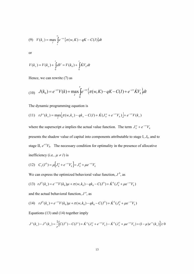
(9) { }∫∞

− −−=τ

ττ π dtICqKKwekV r

I)(),(max)(

or

∫∫ +=+=ττ

τ0

00

)()()( dtVKkVdVkVkV ko&

Hence, we can rewrite (7) as

(10) { }dtVKeICqKKwekVekJ krr

I

r &ττ

ττ π −−− +−−+= ∫ )(),(max)()(0

0

The dynamic programming equation is

(11) ⎣ ⎦ )()()(),(max)( τττπ kVeVeJKICqkkwkrJ r

kra

kooIoa −− +++−−= &

where the superscript a implies the actual value function. The term kra

k VeJ τ−+

presents the shadow value of capital into components attributable to stage I, Jk, and to

stage II, e-rτVk. The necessary condition for optimality in the presence of allocative

inefficiency (i.e., μ ≠ 1) is

(12) [ ] krb

kkra

kb

I VeJVeJIC ττ μμ −− +=+=)(

We can express the optimized behavioral value function, J b, as

(13) )()(),()()( 000 krb

kbbr

ob VeJKICqkkwkVekrJ ττ μπμ −− ++−−+= &

and the actual behavioral function, J a, as

(14) )()(),()()( 000 krb

kbbr

ob VeJKICqkkwkVekrJ ττ μπμ −− ++−−+= &

Equations (13) and (14) together imply

[ ] 0)()1()()()()(1)()( ≥−++−++−=− −−o

rk

rbk

bk

rak

aabo

bo

a keVeJKVeJKICICr

kJkJ τττ μμ&&

14

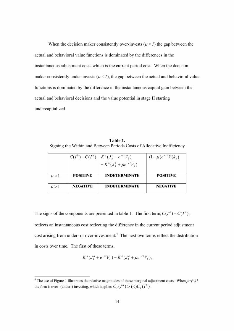
When the decision maker consistently over-invests (μ >1) the gap between the

actual and behavioral value functions is dominated by the differences in the

instantaneous adjustment costs which is the current period cost. When the decision

maker consistently under-invests (μ <1), the gap between the actual and behavioral value

functions is dominated by the difference in the instantaneous capital gain between the

actual and behavioral decisions and the value potential in stage II starting

undercapitalized.

Table 1. Signing the Within and Between Periods Costs of Allocative Inefficiency

)()( ab ICIC −

)(

)(

krb

kb

kra

ka

VeJK

VeJKτ

τ

μ −

−

+−

+&

&

)()1( or kVe τμ −−

1<μ POSITIVE INDETERMINATE POSITIVE

1>μ NEGATIVE INDETERMINATE

NEGATIVE

The signs of the components are presented in table 1. The first term, )()( ab ICIC − ,

reflects an instantaneous cost reflecting the difference in the current period adjustment

cost arising from under- or over-investment.4 The next two terms reflect the distribution

in costs over time. The first of these terms,

)()( krb

kb

kra

ka VeJKVeJK ττ μ −− +−+ && ,

4 The use of Figure 1 illustrates the relative magnitudes of these marginal adjustment costs. When μ>(<)1 the firm is over- (under-) investing, which implies )()()( b

Ia

I ICIC <> .

15

reflects the change in the instantaneous capital gain (or loss) associated with an adding

(or not allocating) another unit of capital. We can decompose this term further to reflect

the impact of the instantaneous capital gain/loss in stage I, bk

bak

a JKJK && − , and impact of

an investment mistake in stage I the instantaneous capital gain/loss in the stage II,

krba VeKK τμ −−− )1)(( && . The second of these terms, )()1( o

r kVe τμ −− , reflects the impact

of stage I inefficiency on the value function in stage II.

A simple graphical illustration is presented in Figure 2. The optimal capital

trajectory is the blue line, K0 A0 A1. Consider the case a mistake is made at time t1 where

μ = μ1 >1 leading to overinvestment in that period. If this overinvestment is expected to

persist indefinitely, then the capital trajectory continues from B0 to B1. The problem

with this characterization of inefficiency is that it is implicitly assumes that there will be

no more mistakes between t1 and the terminal time.

K

time

T t1

K0

A0

B0 A1

B1

Figure 2

16

V. FUTURE DIRECTIONS

Distribution of Trajectories

The shadow value function model starkly illustrates the need to generate the

distribution of trajectories associated with the distribution of inefficiencies over time.

On this score, the approach of Tsionas (2006) can offer a useful starting point. The fuller

extension should also account for the decision processes and choices associated with

choosing the levels of these forcing factors influencing efficiency levels over time. The

first steps in addressing the structural model with a distribution of inefficiency-

influenced trajectories is to specify an equation of motion on how the inefficiency

changes over time. The approach of Ahn, Good and Sickles (2000) can be augmented to

include the structural nature of adjustment and the distributed impact of present

inefficiency into the future. At present, the Ahn, Good and Sickles approach specifies

two of the three essential elements of a structural model: a) production feasibility with

the production function specification, and b) an equation of motion on efficiency change

with the autoregressive error specification. The element that is missing is the behavioral

constraints relating to optimization problem endorsed by the decision maker.

Learning and Efficiency

When looking at the cognitive capacity, the notions of learning and efficiency

come together. Identifying the dynamic-based costs of inefficiency in table 1 is only half

of the story. There are benefits associated with making mistakes and when the benefits

are realized there is evidence of learning taking place.

17

Focusing on learning as an accumulation of knowledge, the acquisition of

additional knowledge necessarily draws on information acquisition. Knowledge plays an

important role in the process of growth by choosing the right things to do (supporting the

selection systems of technologies) and by doing the right things better (the understanding

and execution of an implemented technology). Knowledge has value if one can translate

it into actions or decisions that lead to enhanced cognitive or economic value. Two

fundamental challenges to the process are: a) how does one acquire more knowledge and

b) how does one translate the knowledge gained into action. Unlike most studies of

information and technology decisions which take a recursive approach to modeling

information acquisition then action on that information, Saha et al (1994) and Genius,

Pantzios and Tsouvelekas (2006) jointly model the degree of technology adoption as a

process jointly determined with the decision maker’s information acquisition processes.

The joint determination of these decisions reflects movement toward a long-run

structural measurement of learning and technological decisions, which can then translate

into measuring efficiency gains and innovation gains.

Firm decision makers react to competitive pressures by balancing the trade off

between exploiting the full productive potential of their systems and technologies and

adopting innovations. Both avenues can lead to enhanced profitability. Sustaining

competitiveness over the long run involves attention to both growth prospects: (i)

innovations are needed to keep pushing the competitive envelope, and (ii) efficiency

gains are needed to ensure that implemented technologies can succeed. The effective

management of knowledge and its acquisition (i.e., learning) contributes to both sources

of profitability growth.

18

An emerging direction is to consider the directional distance function approach in

a dynamic context. The start to this conceptualization can be found in Silva and

Stefanou (2007)

}):()),(:{min),,,( 1tttgttgtgtttttg kyVIxkIxyF ∈= −γγγ ,

where this measure computes the maximum equiproportionate variable input reduction

and gross investment expansion in the input requirement set, V(yt: kt), to itself and

0<Fg(yt,xt,It,kt)≤1. Silva and Oude Lansink (2006) present a first venture into this

entirely new area and demonstrate how efficiency measures can be additive measures of

efficiency measures rather than ration measures and allow the separation of the

contribution of individual variable and dynamic factors to inefficiency.

But how learning is modeled in this context needs to be clearly specified. Is the

firm Planning to Learn vs. Planning to Execute. This can influence the inefficiency

measure in terms of modeling decisions as exogenous or endogenous. When the

resources and efforts to mount a significant increase in the base of knowledge are

considerable, the there is also the option value to learn, which can lead to modeling

learning-based adjustment paths.

VI. CONCLUDING COMMENTS

The multiple directions observed in the literature to date to a great extent reflect a trade

off between power of the theory and power of the data. The theory imbedded in

structural models offers power in terms of informing our model specification of

behavioral constraints and error structures as we look to rationalize the data. A

theoretically founded structural model offers the further advantage of extending our

19

models to address related issues in the area of dynamic economic performance such as

productivity growth, capacity utilization, the impact of multiple output production

scenarios and the scope economies they imply. However, the data can often get in the

way and our results can point out some disturbing shortcomings in the power of the

theory-based models. With the emergence of longer panels at the enterprise and plant

levels, we are observing a phenomenon of the persistence of inefficiency; that is, firms

are not necessarily doing things better. We can try to rationalize these results by

focusing on the structural foundations of decisions making or the data-driven modeling

building. For example, is the persistence of inefficiency:

• an artifact of the data in terms of the variable constructions and definitions (a

notorious problem when considering the efficiency of capital assets and whether

they are valued at book value or market value);

• an artifact of the model that is not able to capture all the sources driving

inefficiency; or,

• a shortcoming in our characterization of decision making protocols which related

to the behavioral objectives, or finally, if the cost of inefficiency of some small

level α>0 is not offset by benefit of being perfectly efficient.

The static modeling of inefficiency has made great strides on both theoretical and

methodological fronts over the past 30 years and these efforts are directing future

attention to the measurement of dynamic economic performance. This paper has tried to

lay out some perspectives on the dynamic case, but the landscape is still in need of clear

articulation.

20

References

Abel, A.B., Mankiw, N. G., Summers, L. H., and Zeckhauser, R. J., (1989), "Assessing

Dynamic Efficiency," Review of Economic Studies 56, 1-20. Ahn, S.C., Good, D.H., and Sickles, R.C., (2000), “Estimation of Long-Run Inefficiency

Levels: a Dynamic Frontier Approach," Econometric Reviews, 19, 461-492. Alchian, A., (1959), “Costs and Outputs,” in: M. Abramovitz, The Allocation of

Economic Resources, Essays in Honor of B.F. Haley, Stanford University Press. Atkinson, S. E. and Halvorson, R., (1980), "A Test of Relative and Absolute Price

Efficiency in Regulated Industries," Review of Economics and Statistics 62, 81-88.

Atkinson, S.E. and Cornwell, C., (1994), “Parametric Estimation of Technical and Allocative Inefficiency with Panel Data: A Dual Approach,” International Economic Review 35(1), 231-44.

Bartelsman E. J., and Dhrymes P.J., (1998). “Productivity Dynamics: U.S.

Manufacturing Plants, 1972-1986,” Journal of Productivity Analysis 9, 5-34. Battese, G.E. and Coelli, T.J. (1992), “Frontier Production Functions, Technical

Efficiency and Panel Data,” Journal of Productivity Analysis 3:1/2 (June), 153-69.

Celikkol, P. and Stefanou, S.E., (2004), “Productivity Growth Patterns in U.S. Food

Manufacturing: Case of Meat Products Industry,” Center of Economic Studies, Bureau of Census Working Paper CES-WP-04-04, pp.78.

Cooper, R., Haltiwanger, J. C., and Power, L., (1999). “Machine Replacement and the

Business Cycle: Lumps and Bumps.” American Economic Review 89(4), 921-946.

Cornwell, C., Schmidt, P., and Sickles, R.C., (1990), “Production Frontiers with Cross-

Sectional and Time-Series Variation in Efficiency Levels.” Journal of Econometrics 46(1/2) (October), 185-200.

De Alessi, L., (1967), “The Short Run Revisited,” American Economic Review, 57, 450-

461. Dhrymes, P. J., (1991). “The Structure of Production Technology: Productivity and

Aggregation Effects,” Discussion Paper CES 91-5, Center for Economic Studies, U.S. Bureau of Census, Washington, DC.

Diamond, P., (1965), "National Debt in a Neoclassical Growth Model," American

Economic Review 55(, 1126-1150.

21

Ericson R., and Pakes, A., (1995), “Markov Perfect Industry Dynamics: A Framework

for Empirical Work,” Review of Economic Studies 62(1), 53-82. Färe, R. and Grosskopf, S., (1996), Intertemporal Production Frontiers, Kluwer. Genius, M., Pantzios, C.J., and Tzouvelekas, V., (2003), “Information Acquisition and

Adoption of Technological Innovations,” Working paper, Department of Economics, University of Crete..

Kumbhakar, S. C., (1990), “Production Frontiers, Panel Data, and Time-Varying

Technical Inefficiency,” Journal of Econometrics 46:1/2 (Oct/Nov), 201-12. Kumbhakar, S. C., (1997), “Modeling Allocative Inefficiency in a Translog Cost

Function and Cost Share Equations: An Exact Relationship,” Journal of Econometrics 76:1/2 (Jan/Feb), 351-56.

Kumbhakar, S.C., and Lovell, C.A.K., (2000), Stochastic Frontier Analysis. Cambridge

University Press. Lee, Y.H. And Schmidt, P. (1993), “ Production Frontier Model with Flexible Temporal

Variation in Technical Inefficiency,” in Fried, H.O., Lovell, C.A.K. and Schmidt, S.S., eds., The Measurement of Productive Efficiency: Techniques and Applications. Oxford University Press.

Kleindorfer, G.B., Kleindorfer, P.R., Kriebel, C.H., and Thompson, G., (1975),

“Discrete Optimal Control f Production Plans, Management Science 22 (3) (November), 261-73.

Nemoto, J. and Goto, M., (1999), “Dynamic Data Envelope Analysis: Modeling

Intertemporal Behavior of a Firm in the Presence of Production Inefficiencies, Economics Letters 64, 51-56.

Nemoto, J. and Goto, M., (2003), “Measurement of Dynamic Efficiency in Production:

An Application of Data Envelopment Analysis to Japanese Electric Utilities,” Journal of Productivity Analysis, 19(2/3), pp. 191-210.

Nilsen, O.A. and Schiantarelli, F. (2003), “Zeroes and Lumps in Investment: Empirical

Evidence on Irreversibilities and Nonconvexities,” Review of Economics and Statistics 85(4) (November), 1021-37.

Olley, G. S. and Pakes, A., (1996). “The Dynamics of Productivity in the

Telecommunication Equipment Industry,” Econometrica, 64(6), 1263-97.

22

Pakes, A and McGuire, P., (1994). “Computing Markov-Perfect Nash Equilibria: Numerical Implications of a Dynamic Differentiated Product Model,” RAND Journal of Economics 25(4), 555-89.

Ericson, P. and Pakes A., (1995). “Markov Perfect Industry Dynamics: A Framework for

Empirical Work, Review of Economic Studies 62, 53-82. Rungsuriyawiboon, S. and Stefanou, S.E., (2007), “Dynamic Efficiency Estimation: An

Application to US Electric Utilities,” Journal of Business and Economic Statistics, in press.

Saha, A., Love, A.H. and Schwart, R., (1994), “Adoption of Emerging Technologies

Under Output Uncertainty,” American Journal of Agricultural Economics 76 (May), 386-846.

Sengupta , J.K., (1995), Dynamics of Data Envelope Analysis: Theory of Systems Efficiency, Kluwer.

Sengupta, J.K., (1997), “Persistence of Dynamic Efficiency in Farrell Models,” Applied Economics 29(5), 665-71.

Shephard, R. and Färe, R., (1978), ”Dynamic Theory of Production Correspondences:

Parts I-III,” ORC-78-2 through 78-4, Operations Research Center, University of California, Berkeley.

Silva, E. and Stefanou, S.E., (2003), “Nonparametric Dynamic Production Analysis and

the Theory of Cost, Journal of Productivity Analysis, 19 (January), 5-32. Silva, E. and Stefanou, S.E., (2007), “Nonparametric Dynamic Efficiency Analysis,”

American Journal of Agricultural Economics, in press. Silva, E. and Oude Lansink, A. (2006), “Dynamic Efficiency Measurement: A

Directional Distance Function Approach,” Working Paper, Department of Business Economics, Wageningen University, Netherlands.

Stefanou, S.E., (1989), “The Returns to scale in the long run: the dynamic theory of

cost,” Southern Economic Journal 55, 570-79. Stefanou, S. E. and Saxena, S., (1988), "Education, Experience and Allocative

Efficiency: A Dual Approach," American Journal of Agricultural Economics 70, 338-45.

Thalmann, P., (1996), Tests of Technical Efficiency for the Real World of Firms, Paper

presented Georgia Productivity Workshop I, University of Georgia, October 1994 (revised 1996).

23

Tirole, J., (1985), "Asset Bubbles and Overlapping Generations," Econometrica 53, 1499-1528.

Toda, Y. (1976), "Estimation of a Cost Function When the Cost is not Minimum: The

Case of Soviet Manufacturing Industries, l958-l97l." Review of Economics and Statistics 58, 259-268.

Tsionas, E. G. (2006), "Inference in Dynamic Stochastic Frontier Models", Journal of

Applied Econometrics, 21, 669-676 Vaneman, W. and Triantis, K., (2003), “The Dynamic Production Axioms and System

Dynamics Behaviors: The Foundation for Future Integration,” Journal of Productivity Analysis 19 (January), pp. 93-113.

Vaneman, W. and Triantis, K., (2004), “Evaluating the Productive Efficiency of

Dynamical Systems,” Virginia Tech, System Performance Laboratory. Viner, J., (1931), “Cost Curves and Supply Curves,” Zeitschrift für Nationalökonomie, 23-

46. Reprinted in A.E.A Readings in Price Theory, 1952, Boulding, K.E. and Stigler, G.J., eds., Homewood, IL: Richard D. Irwin.

Weil, P., (1987), "Love They Children: Reflections in the Barro Debt-Neutrality

Theorem," Journal of Monetary Economics 19, 377-391.