Embed Size (px)
Citation preview
Dynamic Analysis of Small Pigs in Space PipelinesM. Saeidbakhsh1, M. Rafeeyan1 and S. Ziaei-Rad2
1 Department of Mechanical Engineering, Yazd University, Yazd - Iran2 Department of Mechanical Engineering, Isfahan University of Technology, Isfahan - Iran
e-mail: [email protected] - [email protected] - [email protected]
Résumé — Analyse dynamique des petits racleurs dans les pipelines spatiaux — Cet essai traite despropriétés dynamiques des petits racleurs (jauges d’inspection des pipelines) dans les pipelines spatiaux.Tout d’abord, les équations différentielles pour l’analyse dynamique des petits racleurs, dont la longueurest réduite, sont développées. Le champ d’écoulement peut avoir un impact considérable sur la trajectoiredu racleur. Au cours de cette étude, l’impact du champ d’écoulement sur la trajectoire du racleur a étéignoré. Il faut partir du principe que la trajectoire du racleur ou l’axe du pipeline est une courbe dansl’espace tridimensionnel. Ensuite, les équations différentielles du mouvement sont combinées et réduitespour obtenir une seule équation différentielle non linéaire par rapport au paramètre de la courbe spatiale.La méthode de Runge-Kutta d’ordre 4 est ensuite utilisée pour résoudre l’équation. L’énergie motrice estconsidérée comme étant dépendante du temps, mais le coefficient de frottement est constant pour plus desimplicité. Les résultats de la simulation montrent que les équations dérivées permettent d’estimerefficacement la position et la vitesse du racleur et les forces auxquelles il est soumis tout au long de sondéplacement.
Abstract — Dynamic Analysis of Small Pigs in Space Pipelines — This paper deals with the dynamicsof small pipeline inspection gauges (pigs) in space pipelines. First, the differential equations for dynamicanalysis of the small pig, whose length is short, are developed. The flow field can significantly influencethe pig’s trajectory. In this research, the effect of the flow field on the pig’s trajectory was ignored. Thepath of the pig or centerline of the pipeline is assumed to be a curve in 3D space. Next, the differentialequations of motion are combined and reduced to only one nonlinear differential equation with respect tothe parameter of the space curve. The fourth-order Runge-Kutta method is then used for solving theequation. The driving force is assumed to be time-dependent, but the coefficient of friction is assumed tobe constant for the sake of simplicity. The simulation results show that the derived equations are effectivefor estimating the position and velocity of the pig and forces acting on it at all time instants of its motion.
Oil & Gas Science and Technology – Rev. IFP, Vol. 64 (2009), No. 2, pp. 155-164Copyright © 2008, Institut français du pétroleDOI: 10.2516/ogst:2008046
Oil & Gas Science and Technology – Rev. IFP, Vol. 64 (2009), No. 2
INTRODUCTION
One of the safest methods to transport oil and gas products isby pipeline. Pipelines transport liquid and gas products ofrefineries to cities. During this transportation, they passthrough rivers, mountains and so on. Therefore, one canassume that their geometry is a space curve in general. Also,most parts of the pipelines are buried in the ground. Hence, apipeline can fail for different reasons such as change incurvature or length, pipe wall corrosion, increase in the pipewall’s roughness, and reduction of the internal diameter. Toprevent these factors and other targets such as cleaning anddewatering, pipelines must be pigged regularly. The toolwhich is used for pigging is called a pipeline inspectiongauge (pig). It is a device which is inserted into a pipelineand travels throughout the pipeline to be inspected. It canalso monitor the physical condition of the pipeline. Theoperation of the pig, regarding the pigging target, depends onits speed and acceleration. An estimation of these parametersis very important before the pigging operation. Selecting thebest pig geometry, estimating its speed, required drivingpressure and the amount of back and forward bypass of fluidare all based on our knowledge about the dynamic behaviorof pigs.
The advent of high-resolution magnetic-based on-lineinspection and monitoring equipment now allows operatorsto thoroughly assess the integrity of a pipeline. In a paper[1], the varieties of pipe-wall defects that can be detectedduring pigging are explained. Some analytical techniquesare summarized and their assessments are discussed. Theincorporation of these methods into condition-monitoringplans is argued, and finally, an overall defect assessmentmethodology is presented. The article [2] is the first in aseries discussing the performance of conventional pipelinepigs. The aim is to provide users, manufacturers andsuppliers with awareness of the advantages and limitationsassociated with conventional pipeline pigging,concentrating on oil and gas applications, such ashydrocarbon pipelines.
A literature survey reveals very few papers dealing withthe dynamic analysis of pigs in pipelines. Most of theresearch results are commercially based or field experience.There are some papers that concern the motion of pigs andtry to estimate the pig dynamics in pipelines. Transient pigmotion through gas and liquid pipelines was presented by[3]. In their study, they assumed that the pig moves in astraight line in the plane. Modeling and simulation for pigflow control in natural gas pipelines was studied by [4]. Thisresearch was also concentrated on straight pipelines. Asimple nonlinear controller for controlling the pig velocitywhen it flows in a natural gas straight pipeline was proposedby [5]. Verification of the theoretical model for analyzingdynamic behavior of the pig from actual pigging waspresented in [6]. In all the previous studies, by assuming a
straight line for pipeline geometry, the governing differentialequations of the flow and dynamic equations of the pig weresolved simultaneously.
A self-drive pipeline pig, which obtains its power from thekinetic energy of fluid flow in a pipe via a turbine and areverse–traverse screw mechanism, has been introduced by[7]. Their proposed pig was designed to move both againstand with the flowing fluid, which makes it different fromconventional pigs, which can only move with the flowingfluid. A dynamic model for the pig was then derived. Basedon the model, the dynamic behavior of the pig under differentconditions was analyzed in detail. In order to verify thevalidity of the dynamic model, a prototype machine andpipe-loop test rig was built, and the experimental dataobtained compared with the theoretical analyses.
Liquid condensation in natural gas transmission pipelines,which commonly occurs due to the thermodynamic andhydrodynamic imperatives, was studied by [8]. Condensationsubjects the gas pipeline to two-phase transport, and thepresence of condensation in gas pipelines dramaticallyaffects their delivery ability and operational modality, and theassociated peripheral facilities. It is therefore imperative forthe pigging simulation in gas-condensate flow lines to betaken into consideration during their design. In their study, anew simplified pigging model was developed for predictingthe pigging operation in gas-condensate horizontal pipelineswith low liquid-loading, which couples the phase behaviormodel with the hydro-thermodynamic model. Theycompared their calculation results with those of the two-phase transient computational code OLGA and concludedthat the proposed pigging model has a good precision andhigh speed in calculation. A review on the pigging simulationmodels in multiphase pipelines has been carried out by [9].
In this paper, the aim is to extend the dynamic analysis ofpigs for space curved pipelines. The extension is based onsome simplifying assumptions such as: the pig is small, thepig/wall friction coefficient is constant and the driving forceis time-dependent. It was also assumed that only a pressuredriving force was acting on the pig. The differentialequations of the pig in the space are derived by Newton’ssecond law. Next, the three governing equations are reducedto one equation with respect to the parameter of the curve.Finally, the Runge-Kutta method is used for solving thederived equation. Three case studies are included to illustratethe application of the new formulation.
1 MATHEMATICAL MODEL
Figure 1 shows the free body diagram of a typical small piginside a space pipeline. The weight of the pig, W, dry frictionforce, f, normal force by the pipe wall, N, and the drivingforce, P, are the forces acting on the pig. These forces ingeneral, as shown in Figure 1, are space vectors. The position
156
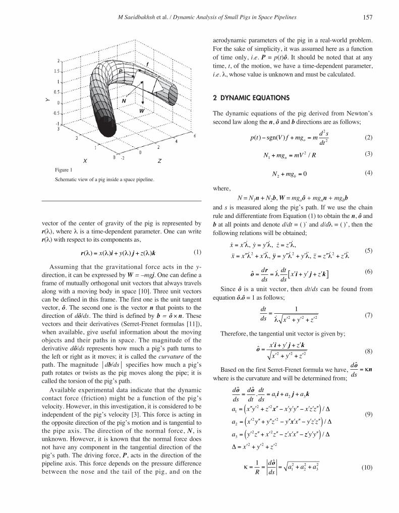
vector of the center of gravity of the pig is represented byr(λ), where λ is a time-dependent parameter. One can writer(λ) with respect to its components as,
(1)
Assuming that the gravitational force acts in the y-direction, it can be expressed by W = –mgj. One can define aframe of mutually orthogonal unit vectors that always travelsalong with a moving body in space [10]. Three unit vectorscan be defined in this frame. The first one is the unit tangentvector, ô. The second one is the vector n that points to thedirection of dô/ds. The third is defined by b = ô × n. Thesevectors and their derivatives (Serret-Frenet formulas [11]),when available, give useful information about the movingobjects and their paths in space. The magnitude of thederivative dô/ds represents how much a pig’s path turns tothe left or right as it moves; it is called the curvature of thepath. The magnitude ⏐db/ds⏐ specifies how much a pig’spath rotates or twists as the pig moves along the pipe; it iscalled the torsion of the pig’s path.
Available experimental data indicate that the dynamiccontact force (friction) might be a function of the pig’svelocity. However, in this investigation, it is considered to beindependent of the pig’s velocity [3]. This force is acting inthe opposite direction of the pig’s motion and is tangential tothe pipe axis. The direction of the normal force, N, isunknown. However, it is known that the normal force doesnot have any component in the tangential direction of thepig’s path. The driving force, P, acts in the direction of thepipeline axis. This force depends on the pressure differencebetween the nose and the tail of the pig, and on the
r i j k( ) ( ) ( ) ( )λ λ λ λ= + +x y z
aerodynamic parameters of the pig in a real-world problem.For the sake of simplicity, it was assumed here as a functionof time only, i.e. P = p(t)ô. It should be noted that at anytime, t, of the motion, we have a time-dependent parameter,i.e. λ, whose value is unknown and must be calculated.
2 DYNAMIC EQUATIONS
The dynamic equations of the pig derived from Newton’ssecond law along the n, ô and b directions are as follows;
(2)
(3)
(4)
where,
N = N1n + N2b, W = mgoô + mgnn + mgbband s is measured along the pig’s path. If we use the chainrule and differentiate from Equation (1) to obtain the n, ô andb at all points and denote d/dt = ( )⋅ and d/dλ = ( )’, then thefollowing relations will be obtained;
(5)
(6)
Since ô is a unit vector, then dt/ds can be found fromequation ô.ô = 1 as follows;
(7)
Therefore, the tangential unit vector is given by;
(8)
Based on the first Serret-Frenet formula we have, where is the curvature and will be determined from;
(9)
(10) κ = = = + +
112
22
32
R
d
dsa a a
o
d
ds
d
dt
dt
dsa a a
a x y z
ˆ ˆ.
o o i j k= = + +
= ′′ ′ + ′ ′′
1 2 3
12 2 xx x y y x z z
a x y y z y
− ′ ′ ′′ − ′ ′ ′′( )= ′ ′′ + ′′ ′ − ′′ ′
/ Δ
22 2 xx x y z z
a y z x z z x x
′′ − ′ ′ ′′( )= ′ ′′ + ′ ′′ − ′ ′ ′′ − ′
/ Δ
32 2 zz y y
x y z
′ ′′( )= ′ + ′ + ′
/ Δ
Δ 2 2 2
d
ds
o n= κ
o i j k=
′ + ′ + ′
′ + ′ + ′
x y z
x y z2 2 2
dt
ds x y z=
′ + ′ + ′
12 2 2�λ
o r i j k= = ′ + ′ + ′[ ]d
ds
dt
dsx y z�λ
� � � � � �
�� � �� ��
x x y y z z
x x x
= ′ = ′ = ′
= ′′ + ′
λ λ λ
λ λ
, , ,
,2 yy y y z z z= ′′ + ′ = ′′ + ′� �� �� � ��λ λ λ λ2 2,
N mgb2 0+ =
N mg mV Rn12+ = /
p t V f mg md s
dto( ) sgn( )− + =2
2
M Saeidbakhsh et al. / Dynamic Analysis of Small Pigs in Space Pipelines 157
Y
X Z
W
Pf
N
Figure 1
Schematic view of a pig inside a space pipeline.
Oil & Gas Science and Technology – Rev. IFP, Vol. 64 (2009), No. 2
Also, the normal unit vector n can be obtained fromEquation (9)
(11)
The second normal unit vector is derived from the outercross-product of ô and n, i.e.
(12)
Since the projection of the vector V1 on V2 is equal toV1.V2/ V1 ⏐V2⏐ then gn, go and gb can be obtained as:
(13)
(14)
(15)
Now, one needs to calculate the remaining unknown termsin Equations (2) to (5), i.e.,
(16)
Substituting Equations (13) and (14) and the magnitude of(16) in (3) and (4) results in the components of normalforces:
(17)
(18)
(19)
Finally, substituting Equations (19) and (16) in Equation (2)results in:
(20)
p t V m
a a aga
a a a( ) sgn( ).−
+ + ++ +
⎛
⎝μ
Δ 12
22
32 2
12
22
32
⎜⎜⎜
⎞
⎠⎟⎟
+′ − ′
+ +
⎛
⎝⎜⎜
⎞
⎠⎟⎟
2
3 1
12
22
32
2
g a x a z
a a a
( )
(Δ
⎧⎧
⎨
⎪⎪⎪
⎩
⎪⎪⎪
⎫
⎬
⎪⎪⎪
⎭
⎪⎪⎪
−′
= ′ ′′ +
1 2
2
/
(mgy m
x xΔ Δ
� ��λ λλ λ λ λ λ′ + ′ ′′ + ′ + ′ ′′ + ′{ }x y y y z z z) ( ) ( )� �� � ��2 2
N N= + =N N f12
22 , μ
Nmg a x a z
a a a2
3 1
12
22
32
= −′ − ′
+ +
( )
(Δ
N m a a aga
a a a1 1
222
32 2
12
22
32
= + + ++ +
[ ]�λΔ
V r i j k= = ′ + ′ + ′� �( ) ( )λ λx y z
ggy
x y zo = −
′
′ + ′ + ′2 2 2
gg a x a z
a a ab =
′ − ′
+ +
( )
( )3 1
12
22
32Δ
gga
a a an = −
+ +2
12
22
32
b o n
i
= × =+ +( )
′ − ′( ) − ′ − ′
ˆ 1
12
22
32
3 2 3 1
Δ a a a
a y a z a x a zz a x a z( ) + ′ − ′( )⎡⎣ ⎤⎦j k2 1
n i j k= + +( )a a a1 2 3 / κ
The above equation is a nonlinear differential equationwith respect to λ, which can be solved by a numericaltechnique such as Runge-Kutta based on initial conditions.When parameter λ is determined in each time instant t, thenthe position and the velocity of the pig can be calculatedeasily.
3 NUMERICAL STUDIES
In order to show the validity of the developed equations,three case studies were designed and solved by the proposednumerical technique.
3.1 Case 1
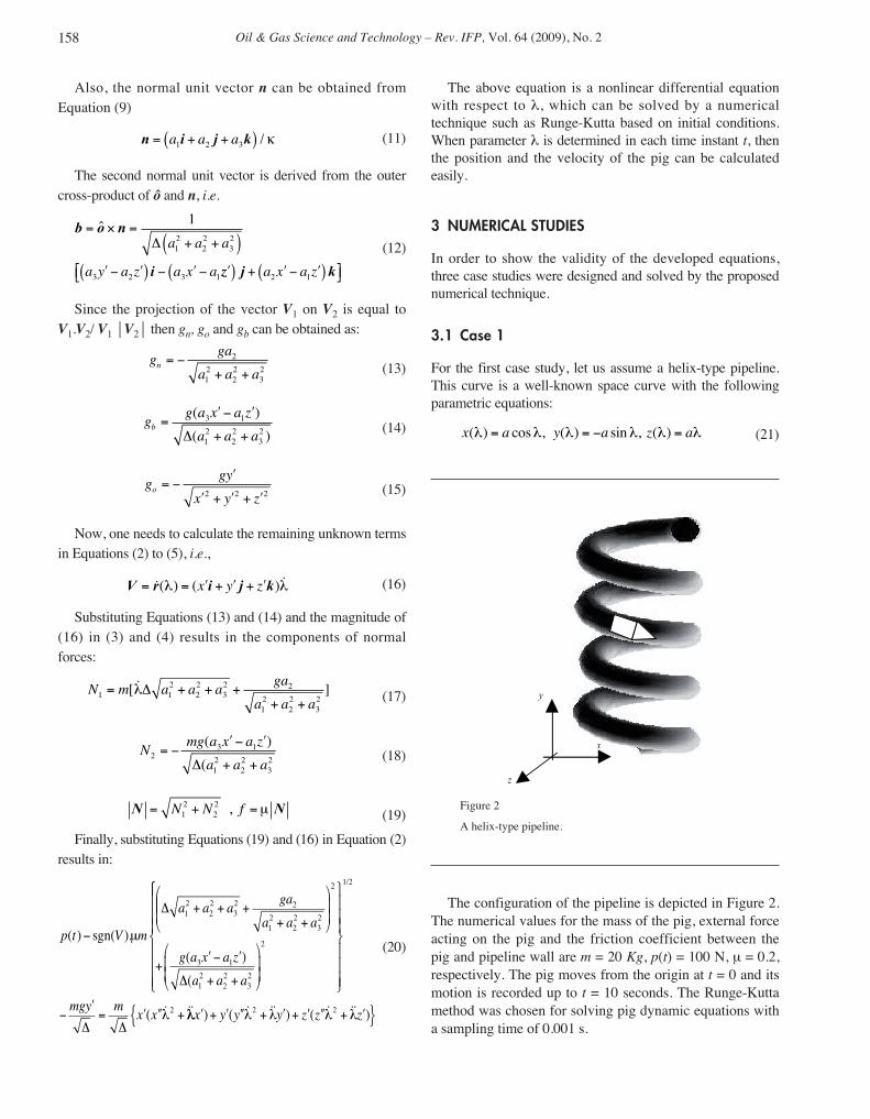
For the first case study, let us assume a helix-type pipeline.This curve is a well-known space curve with the followingparametric equations:
(21)x a y a z a( ) cos , ( ) sin , ( )λ λ λ λ λ λ= = − =
The configuration of the pipeline is depicted in Figure 2.The numerical values for the mass of the pig, external forceacting on the pig and the friction coefficient between thepig and pipeline wall are m = 20 Kg, p(t) = 100 N, μ = 0.2,respectively. The pig moves from the origin at t = 0 and itsmotion is recorded up to t = 10 seconds. The Runge-Kuttamethod was chosen for solving pig dynamic equations witha sampling time of 0.001 s.
158
y
x
z
Figure 2
A helix-type pipeline.
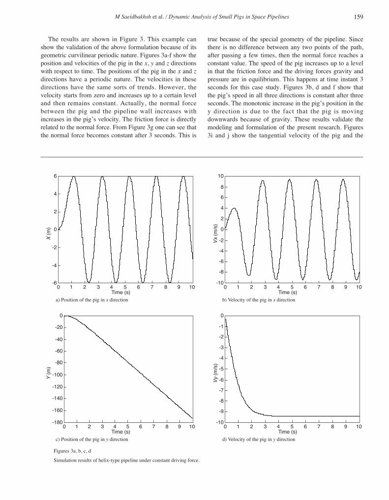
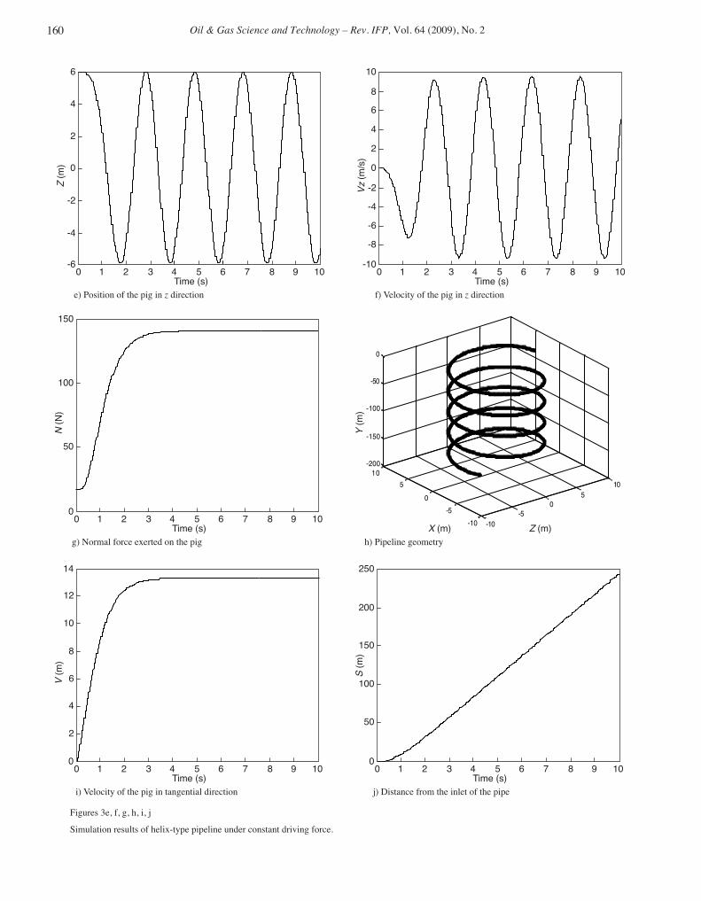
The results are shown in Figure 3. This example canshow the validation of the above formulation because of itsgeometric curvilinear periodic nature. Figures 3a-f show theposition and velocities of the pig in the x, y and z directionswith respect to time. The positions of the pig in the x and zdirections have a periodic nature. The velocities in thesedirections have the same sorts of trends. However, thevelocity starts from zero and increases up to a certain leveland then remains constant. Actually, the normal forcebetween the pig and the pipeline wall increases withincreases in the pig’s velocity. The friction force is directlyrelated to the normal force. From Figure 3g one can see thatthe normal force becomes constant after 3 seconds. This is
true because of the special geometry of the pipeline. Sincethere is no difference between any two points of the path,after passing a few times, then the normal force reaches aconstant value. The speed of the pig increases up to a levelin that the friction force and the driving forces gravity andpressure are in equilibrium. This happens at time instant 3seconds for this case study. Figures 3b, d and f show thatthe pig’s speed in all three directions is constant after threeseconds. The monotonic increase in the pig’s position in they direction is due to the fact that the pig is movingdownwards because of gravity. These results validate themodeling and formulation of the present research. Figures3i and j show the tangential velocity of the pig and the
M Saeidbakhsh et al. / Dynamic Analysis of Small Pigs in Space Pipelines 159
-180109876543210
Y (
m)
0
-20
-40
-60
-80
-100
-120
-140
-160
c) Position of the pig in y direction
Time (s)
-10109876543210
Vy
(m/s
)
0
-1
-2
-3
-4
-5
-6
-7
-8
-9
d) Velocity of the pig in y direction
Time (s)
-6109876543210
X (
m)
6
-4
-2
0
2
4
a) Position of the pig in x direction
Time (s)
-10109876543210
Vx
(m/s
)
10
8
6
4
2
0
-2
-4
-6
-8
b) Velocity of the pig in x direction
Time (s)
Figures 3a, b, c, d
Simulation results of helix-type pipeline under constant driving force.
Oil & Gas Science and Technology – Rev. IFP, Vol. 64 (2009), No. 2160
-6109876543210
Z (
m)
6
-4
-2
0
2
4
e) Position of the pig in z direction
Time (s)
-10109876543210
Vz
(m/s
)
10
8
6
4
2
0
-2
-4
-6
-8
f) Velocity of the pig in z direction
Time (s)
-10-5
05
10
-10
-5
0
5
10-200
-150
-100
-50
0
0109876543210
N (
N)
150
100
50
g) Normal force exerted on the pig
Time (s)
Y (
m)
h) Pipeline geometry
X (m) Z (m)
0109876543210
250
50
100
150
200
i) Velocity of the pig in tangential direction
Time (s)
S (
m)
0109876543210
V (
m)
14
2
4
6
8
10
12
j) Distance from the inlet of the pipe
Time (s)
Figures 3e, f, g, h, i, j
Simulation results of helix-type pipeline under constant driving force.
distance of the pig from the pipeline inlet, respectively. Thetangential velocity reaches 13.5 m/s and then remainsconstant. The distance that the pig moves inside the pipelineis around 240 m after 10 seconds.
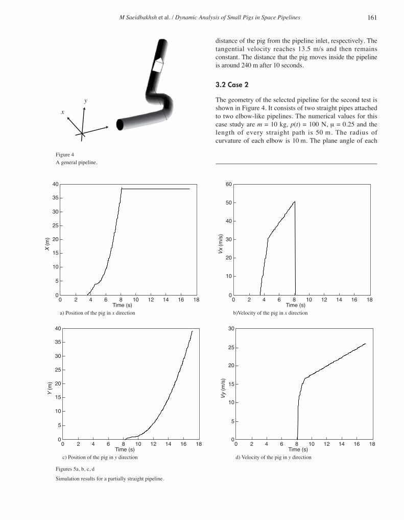
3.2 Case 2
The geometry of the selected pipeline for the second test isshown in Figure 4. It consists of two straight pipes attachedto two elbow-like pipelines. The numerical values for thiscase study are m = 10 kg, p(t) = 100 N, μ = 0.25 and thelength of every straight path is 50 m. The radius ofcurvature of each elbow is 10 m. The plane angle of each
M Saeidbakhsh et al. / Dynamic Analysis of Small Pigs in Space Pipelines 161
x
y
0181614121086420
X (
m)
40
5
10
15
20
25
30
35
a) Position of the pig in x direction
Time (s)
0181614121086420
Vx
(m/s
)
60
10
20
30
40
50
b)Velocity of the pig in x direction
Time (s)
0181614121086420
Y (
m)
40
5
10
15
20
25
30
35
c) Position of the pig in y direction
Time (s)
0181614121086420
Vy
(m/s
)
30
5
10
15
20
25
d) Velocity of the pig in y direction
Time (s)
Figure 4
A general pipeline.
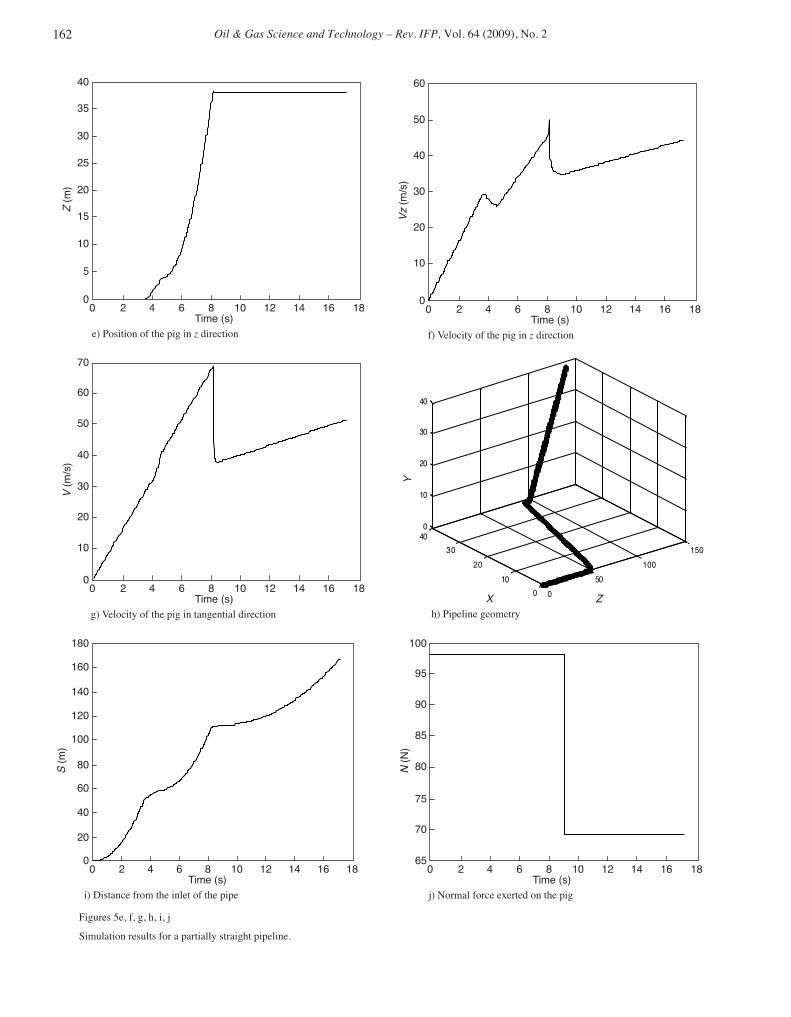
Figures 5a, b, c, d
Simulation results for a partially straight pipeline.
Oil & Gas Science and Technology – Rev. IFP, Vol. 64 (2009), No. 2162
0181614121086420
Z (
m)
40
5
10
15
20
25
30
35
e) Position of the pig in z direction
Time (s)
0181614121086420
60
10
20
30
40
50
Vz
(m/s
)
f) Velocity of the pig in z direction
Time (s)
0181614121086420
V (
m/s
)
70
10
20
30
40
50
60
g) Velocity of the pig in tangential direction
Time (s) 0
50
100
150
0
10
20
30
400
10
20
30
40
X Z
Y
h) Pipeline geometry
0181614121086420
S (
m)
180
20
40
60
80
100
120
140
160
i) Distance from the inlet of the pipe
Time (s)
65181614121086420
N (
N)
100
70
75
80
85
90
95
j) Normal force exerted on the pig
Time (s)
Figures 5e, f, g, h, i, j
Simulation results for a partially straight pipeline.
M Saeidbakhsh et al. / Dynamic Analysis of Small Pigs in Space Pipelines 163
a) Velocity of the pig in tangential direction
Time (s)
0109876543210
V (
m)
14
2
4
6
8
10
12
0109876543210
140
20
40
60
80
100
120
N (
N)
b) Normal force exerted on the pig
Time (s)
c) Distance from the inlet of the pipe
Time (s)
0109 876543210
S (
m)
180
20
40
60
80
100
120
140
160
-10-5
05
10
-10
-5
0
5
10-150
-100
-50
0
Y (
m)
d) Pipeline geometry
X (m) Z (m)
e) Velocity of the pig in x direction
Time (s)
-10109876543210
Vx
(m/s
)
10
-8
-6
-4
-2
0
2
4
6
8
f) Velocity of the pig in y direction
Time (s)
-10109876543210
Vy
(m/s
)
0
-9
-8
-7
-6
-5
-4
-3
-2
-1
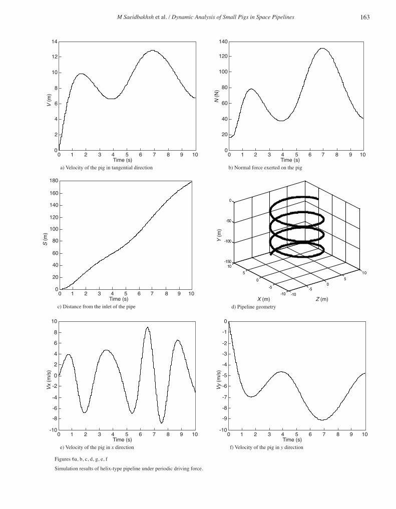
Figures 6a, b, c, d, g, e, f
Simulation results of helix-type pipeline under periodic driving force.
Oil & Gas Science and Technology – Rev. IFP, Vol. 64 (2009), No. 2
elbow is 45°. The aim is to test the ability of the developedsoftware to predict the displacement of the pig through apipeline with elbows connecting straight segments. Thepig’s motion inside the pipeline was determined for a timeinterval of 20 seconds. The Runge-Kutta method with asampling time of 0.02 s was used for this case study.
The results are depicted in Figure 5. Figures 5a-j presentthe similar results for a pipeline with practical typegeometry. This geometry is more complex than case 1because of discontinuity in geometry curvature at the jointof the straight pipe to the elbow. The developed code canalso handle this complex type geometry. For this reason,most of the results in this case such as the position andvelocities of the pig have some discontinuity at the joints.In other words, since the function of the centerline curve ofthis pipe is not thoroughly unique, then there are somejumps in velocities of the pig (Fig. 5b, d, f, g).
3.3 Case 3
Let us consider case 1 again. The only difference is the drivingforce is assumed to be time-dependent, i.e. p(t) = 100 cos t N.This selection can show the validation of the computerprogram because of the periodic nature of the driving force.The results of this case are depicted in Figure 6a-f. Theperiodic nature of the force causes the change in tangentialvelocity and normal force exerted on the pig in comparisonwith case 1.
CONCLUSIONS
This paper presents a computational method using Newton’ssecond law and the Serret-Frenet formula for dynamicanalysis of pigs in space curves. The method is limited bytime-dependent forces on the pig. The pig’s displacement andthe flow field are assumed to be decoupled. In other words,the influence of the flow field on the pig’s trajectory wasignored.
Three numerical case studies were selected to validate theproposed procedure of the paper. The results from the firstcase are in agreement with the physical nature of the problem.
The second case study is an example of a real-world pipeline. Due to the discontinuous nature of the connectionbetween the elbows and straight pipes, there arediscontinuities in the velocity of the pig during its motion inthe pipe. These jumps can exert high value forces on the pipe
at the connection points when the pig moves along thepipeline. In order to avoid these forces, the differencebetween the curvatures of the connected segments should beas small as possible.
The third case study, which has a time-dependent drivingforce, validated the proposed procedure of the paper for thiscase.
This research was the first effort in realizing a new idea. Itis expected that the present approach can be developed insuch a manner as to include the flow field in its formulation,and become more applicable in speed control of the pig inspace pipelines in the next study.
REFERENCES
1 Hopkins P. (1992) The assessment of pipeline defects duringpigging operations, in Pipeline Pigging Technology, TiratsooJ.N.H. (ed.), Gulf Professional Publishing, 2nd ed., pp. 303-324.
2 Short G.C. (1992) Conventional pipeline pigging technology:part 1 - Challenges to the industry, Pipes Pipelines Int. 37, 3,8-11.
3 Nieckele A.O., Braga A.M.B., Azevedo L.F.A. (2001) Transientpig motion through gas and liquid pipelines, J. Energ. Resour.ASME 123, 260-269.
4 Nguyen T.T., Kim S.B., Yoo H.R., Rho Y.W. (2001) Modelingand simulation for pig flow control in natural gas pipeline,KSME Int. J. 15, 8, 1165-1173.
5 Nguyen T.T., Yoo H.R., Rho Y.W., Kim S.B. (2001) Speedcontrol of pig bypass flow in natural gas pipeline, InternationalSymposium on Industrial Electronics, Pusan, Korea, June 12-16.
6 Kim D.K., Cho S.H., Park S.S. (2003) Verification of thetheoretical model for analyzing dynamic behavior of the PIGfrom actual pigging, KSME Int. J. 17, 9, 1349-1357.
7 Hu Z., Appleton E. (2005) Dynamic characteristics of a novelself-drive pipeline pig, IEEE T. Robotics Autom. 21, 5, 781-789.
8 Xiao-Xuan X., Gong J. (2005) Pigging simulation for horizontalgas-condensate pipelines with low-liquid loading, J. Petrol. Sci.Eng. 48, 272-280.
9 Xu X.-X., Gong J., Deng D.M. (2003) A review of piggingmodel in multiphase pipelines, China Offshore Oil Gas 15, 4,21-24.
10 Thomas G.B., Ross JR., Finney L. (1996) Calculus and AnalyticGeometry, Addison-Wesley Publishing Company, 9th ed.
11 Sokolnikoff I.S. (1964) Tensor Analysis, John Wiley and Sons,New York.
Final manuscript received in May 2008Published online in October 2008
164
Copyright © 2008 Institut français du pétrolePermission to make digital or hard copies of part or all of this work for personal or classroom use is granted without fee provided that copies are not madeor distributed for profit or commercial advantage and that copies bear this notice and the full citation on the first page. Copyrights for components of thiswork owned by others than IFP must be honored. Abstracting with credit is permitted. To copy otherwise, to republish, to post on servers, or to redistributeto lists, requires prior specific permission and/or a fee: Request permission from Documentation, Institut français du pétrole, fax. +33 1 47 52 70 78, or [email protected].