Embed Size (px)
Citation preview

IntroductionHidden Markov Models
Wrap-Up
Dynamic Approaches: The Hidden MarkovModel
Davide Bacciu
Dipartimento di InformaticaUniversità di [email protected]
Machine Learning: Neural Networks and Advanced Models(AA2)

IntroductionHidden Markov Models
Wrap-Up
Last Lecture RefresherLecture Plan
Inference as Message Passing
How to infer the distribution P(Xunk |Xobs) of a number ofrandom variables Xunk in the graphical model, given theobserved values of other variables Xobs
Directed and undirectedmodels of fixed structure
Exact inferencePassing messages (vectors ofinformation) on the structure ofthe graphical model following apropagation directionWorks for chains, trees and canbe used in (some) graphs
Approximated inference can useapproximations of the distribution(variational) or can estimate itsexpectation using examples(sampling)

IntroductionHidden Markov Models
Wrap-Up
Last Lecture RefresherLecture Plan
Today’s Lecture
Exact inference on a chain with observed and unobservedvariablesA probabilistic model for sequences: Hidden MarkovModels (HMMs)Using inference to learn: the Expectation-Maximizationalgorithm for HMMsGraphical models with varying structure: DynamicBayesian NetworksApplication examples

IntroductionHidden Markov Models
Wrap-Up
Last Lecture RefresherLecture Plan
Sequences
A sequence y is a collection of observations yt where trepresent the position of the element according to a(complete) order (e.g. time)Reference population is a set of i.i.d sequences y1, . . . ,yN
Different sequences y1, . . . ,yN generally have differentlengths T 1, . . . ,T N

IntroductionHidden Markov Models
Wrap-Up
Last Lecture RefresherLecture Plan
Sequences in Speech Processing

IntroductionHidden Markov Models
Wrap-Up
Last Lecture RefresherLecture Plan
Sequences in Biology

IntroductionHidden Markov Models
Wrap-Up
Generative models for sequencesLearning and Inference in HMMMax-Product Inference in HMM
Markov Chain
First-Order Markov ChainDirected graphical model for sequences s.t. element Xt onlydepends on its predecessor in the sequence
Joint probability factorizes as
P(X) = P(X1, . . . ,XT ) = P(X1)T∏
t=2
P(Xt |Xt−1)
P(Xt |Xt−1) is the transition distribution; P(X1) is the priordistributionGeneral form: an L-th order Markov chain is such that Xtdepends on L predecessors
P(Xt |Xt−1, . . . ,Xt−L)

IntroductionHidden Markov Models
Wrap-Up
Generative models for sequencesLearning and Inference in HMMMax-Product Inference in HMM
Observed Markov Chains
Can we use a Markov chain to model the relationship betweenobserved elements in a sequence?
Of course yes, but...
Does it make sense to represent P(is|cat)?

IntroductionHidden Markov Models
Wrap-Up
Generative models for sequencesLearning and Inference in HMMMax-Product Inference in HMM
Hidden Markov Model (HMM) (I)
Stochastic process where transition dynamics is disentangledfrom observations generated by the process
State transition is an unobserved (hidden/latent) processcharacterized by the hidden state variables St
St are often discrete with value in {1, . . . ,C}Multinomial state transition and prior probability(stationariety assumption)
Aij = P(St = i |St−1 = j) and πi = P(St = i)

IntroductionHidden Markov Models
Wrap-Up
Generative models for sequencesLearning and Inference in HMMMax-Product Inference in HMM
Hidden Markov Model (HMM) (II)
Stochastic process where transition dynamics is disentangledfrom observations generated by the process
Observations are generated by the emission distribution
bi(yt) = P(Yt = yt |St = i)
IntroductionHidden Markov Models
Wrap-Up
Generative models for sequencesLearning and Inference in HMMMax-Product Inference in HMM
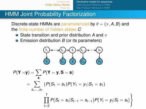
HMM Joint Probability Factorization
Discrete-state HMMs are parameterized by θ = (π,A,B) andthe finite number of hidden states C
State transition and prior distribution A and πEmission distribution B (or its parameters)
P(Y =y) =∑
s
P(Y = y,S = s)
=∑
s1,...,sT
{P(S1 = s1)P(Y1 = y1|S1 = s1)
T∏t=2
P(St = st |St−1 = st−1)P(Yt = yt |St = st)
}

IntroductionHidden Markov Models
Wrap-Up
Generative models for sequencesLearning and Inference in HMMMax-Product Inference in HMM
HMMs as a Recursive Model
A graphical framework describing how contextual information isrecursively encoded by both probabilistic and neural models
Indicates that the hidden state St attime t is dependent on contextinformation from
The previous time step s−1
Two time steps earlier s−2
...
When applying the recursive model to asequence (unfolding), it generates thecorresponding directed graphical model

IntroductionHidden Markov Models
Wrap-Up
Generative models for sequencesLearning and Inference in HMMMax-Product Inference in HMM
3 Notable Inference Problems
Definition (Smoothing)
Given a model θ and an observed sequence y, determine thedistribution of the t-th hidden state P(St |Y = y, θ)
Definition (Learning)
Given a dataset of N observed sequences D = {y1, . . . ,yN}and the number of hidden states C, find the parameters π, Aand B that maximize the probability of model θ = {π,A,B}having generated the sequences in D
Definition (Optimal State Assignment)
Given a model θ and an observed sequence y, find an optimalstate assignment s = s∗1, . . . , s
∗T for the hidden Markov chain

IntroductionHidden Markov Models
Wrap-Up
Generative models for sequencesLearning and Inference in HMMMax-Product Inference in HMM
Forward-Backward Algorithm
Smoothing - How do we determine the posterior P(St = i |y)?Exploit factorization
P(St = i |y) ∝P(St = i ,y) = P(St = i ,Y1:t ,Yt+1:T )
= P(St = i ,Y1:t)P(Yt+1:T |St = i) = αt(i)βt(i)
α-term computed as part of forward recursion (α1(i) = bi(y1)πi )
αt(i) = P(St = i ,Y1:t) = bi(yt)C∑
j=1
Aijαt−1(j)
β-term computed as part of backward recursion (βT (i) = 1, ∀i)
βt(j) = P(Yt+1:T |St = j) =C∑
i=1
bi(yt+1)βt+1(i)Aij

IntroductionHidden Markov Models
Wrap-Up
Generative models for sequencesLearning and Inference in HMMMax-Product Inference in HMM
Deja vu
Doesn’t the Forward-Backward algorithm look strangelyfamiliar?
αt ≡ µα(Xn)→ forward message
µα(Xn)︸ ︷︷ ︸αt (i)
=∑Xn−1︸︷︷︸∑C
j=1
ψ(Xn−1,Xn)︸ ︷︷ ︸bi (yt )Aij
µα(Xn−1)︸ ︷︷ ︸αt−1(j)
βt ≡ µβ(Xn)→ backward message
µβ(Xn)︸ ︷︷ ︸βt (j)
=∑Xn+1︸︷︷︸∑C
i=1
ψ(Xn,Xn+1)︸ ︷︷ ︸bi (yt+1)Aij
µβ(Xn+1)︸ ︷︷ ︸βt+1(i)

IntroductionHidden Markov Models
Wrap-Up
Generative models for sequencesLearning and Inference in HMMMax-Product Inference in HMM
Learning in HMM
Learning HMM parameters θ = (π,A,B) by maximum likelihood
L(θ) = logN∏
n=1
P(Yn|θ)
= logN∏
n=1
∑sn
1 ,...,snTn
P(Sn1)P(Y n
1 |Sn1)
Tn∏t=2
P(Snt |Sn
t−1)P(Y nt |Sn
t )
How can we deal with the unobserved random variables Stand the nasty summation in the log?Expectation-Maximization algorithm
Maximization of the complete likelihood Lc(θ)Completed with indicator variables
znti =
{1 if n-th chain is in state i at time t
0 otherwise
IntroductionHidden Markov Models
Wrap-Up
Generative models for sequencesLearning and Inference in HMMMax-Product Inference in HMM
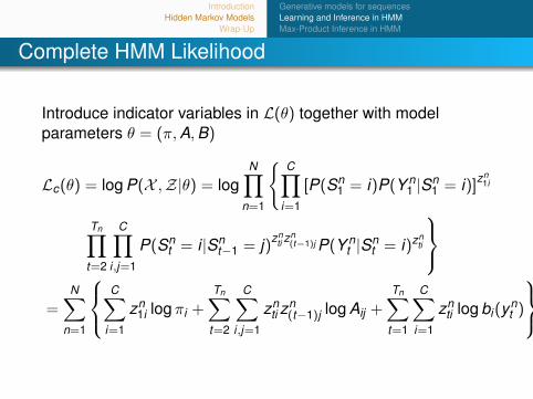
Complete HMM Likelihood
Introduce indicator variables in L(θ) together with modelparameters θ = (π,A,B)
Lc(θ) = log P(X ,Z|θ) = logN∏
n=1
{C∏
i=1
[P(Sn1 = i)P(Y n
1 |Sn1 = i)]z
n1i
Tn∏t=2
C∏i,j=1
P(Snt = i |Sn
t−1 = j)znti z
n(t−1)j P(Y n
t |Snt = i)zn
ti
=
N∑n=1
C∑
i=1
zn1i logπi +
Tn∑t=2
C∑i,j=1
znti z
n(t−1)j log Aij +
Tn∑t=1
C∑i=1
znti log bi(yn
t )

IntroductionHidden Markov Models
Wrap-Up
Generative models for sequencesLearning and Inference in HMMMax-Product Inference in HMM
Expectation-Maximization
A 2-step iterative algorithm for the maximization of completelikelihood Lc(θ) w.r.t. model parameters θ
E-Step: Given the current estimate of the modelparameters θ(t), compute
Q(t+1)(θ|θ(t)) = EZ|X ,θ(t) [log P(X ,Z|θ)]
M-Step: Find the new estimate of the model parameters
θ(t+1) = arg maxθ
Q(t+1)(θ|θ(t))
Iterate 2 steps until |Lc(θ)it −Lc(θ)
it−1| < ε (or stop if maximumnumber of iterations is reached)

IntroductionHidden Markov Models
Wrap-Up
Generative models for sequencesLearning and Inference in HMMMax-Product Inference in HMM
E-Step (I)
Compute the expected value expectation of the completelog-likelihood w.r.t indicator variables zn
ti assuming (estimated)parameters θt = (πt ,At ,Bt) fixed at time t (i.e. constants)
Q(t+1)(θ|θ(t)) = EZ|X ,θ(t) [log P(X ,Z|θ)]
Expectation w.r.t a (discrete) random variable z is
Ez [Z ] =∑
z
z · P(Z = z)
To compute the conditional expectation Q(t+1)(θ|θ(t)) for thecomplete HMM log-likelihood we need to estimate
EZ|Y,θ(k) [zti ] = P(St = i |y)
EZ|Y,θ(k) [ztiz(t−1)j ] = P(St = i ,St−1 = j |Y)

IntroductionHidden Markov Models
Wrap-Up
Generative models for sequencesLearning and Inference in HMMMax-Product Inference in HMM
E-Step (II)
We know how to compute the posteriors by theforward-backward algorithm!
γt(i) = P(St = i |Y) = αt(i)βt(i)∑Cj=1 αt(j)βt(j)
γt ,t−1(i , j) = P(St = i ,St−1 = j |Y) =αt−1(j)Aijbi(yt)βt(i)∑C
m,l=1 αt−1(m)Almbl(yt)βt(l)

IntroductionHidden Markov Models
Wrap-Up
Generative models for sequencesLearning and Inference in HMMMax-Product Inference in HMM
M-Step (I)
Solve the optimization problem
θ(t+1) = arg maxθ
Q(t+1)(θ|θ(t))
using the information computed at the E-Step (the posteriors).How?
As usual∂Q(t+1)(θ|θ(t))
∂θ
where θ = (π,A,B) are now variables.
AttentionParameters can be distributions⇒ need to preservesum-to-one constraints (Lagrange Multipliers)

IntroductionHidden Markov Models
Wrap-Up
Generative models for sequencesLearning and Inference in HMMMax-Product Inference in HMM
M-Step (II)
State distributions
Aij =
∑Nn=1
∑T n
t=2 γnt ,t−1(i , j)∑N
n=1∑T n
t=2 γnt−1(j)
and πi =
∑Nn=1 γ
n1(i)
N
Emission distribution (multinomial)
Bki =
∑Nn=1
∑Tnt=1 γ
nt (i)δ(yt = k)∑N
n=1∑Tn
t=1 γnt (i)
where δ(·) is the indicator function for emission symbols k

IntroductionHidden Markov Models
Wrap-Up
Generative models for sequencesLearning and Inference in HMMMax-Product Inference in HMM
Decoding Problem
Find the optimal hidden state assignement s = s∗1, . . . , s∗T
for an observed sequence y given a trained HMMNo unique interpretation of the problem
Identify the single hidden states st that maximize theposterior
s∗t = arg max
i=1,...,CP(St = i |Y)
Find the most likely joint hidden state assignment
s∗ = arg maxs
P(Y,S = s)
The last problem is addressed by the Viterbi algorithm

IntroductionHidden Markov Models
Wrap-Up
Generative models for sequencesLearning and Inference in HMMMax-Product Inference in HMM
Viterbi Algorithm
An efficient dynamic programming algorithm based on abackward-forward recursion
An example of a max-product message passing algorithm
Recursive backward term
εt−1(st−1) = maxst
P(Yt |St = st)P(St = st |St−1 = st−1)εt(st),
Root optimal state
s∗1 = arg maxs
P(Yt |S1 = s)P(S1 = s1)ε1(s).
Recursive forward optimal state
s∗t = arg maxs
P(Yt |St = s)P(St = s|St−1 = s∗t−1)εt(s).

IntroductionHidden Markov Models
Wrap-Up
ApplicationsDynamic Bayesian NetworksConclusion
Input-Output Hidden Markov Models
Translate an input sequence into an output sequence(transduction)State transition and emissions depend on inputobservations (input-driven)Recursive model highlights analogy with recurrent neuralnetworks
IntroductionHidden Markov Models
Wrap-Up
ApplicationsDynamic Bayesian NetworksConclusion
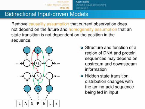
Bidirectional Input-driven Models
Remove causality assumption that current observation doesnot depend on the future and homogeneity assumption that anstate transition is not dependent on the position in thesequence
Structure and function of aregion of DNA and proteinsequences may depend onupstream and downstreaminformationHidden state transitiondistribution changes withthe amino-acid sequencebeing fed in input

IntroductionHidden Markov Models
Wrap-Up
ApplicationsDynamic Bayesian NetworksConclusion
Coupled HMM
Describing interacting processes whose observations followdifferent dynamics while the underlying generative processesare interlaced

IntroductionHidden Markov Models
Wrap-Up
ApplicationsDynamic Bayesian NetworksConclusion
Dynamic Bayesian Networks
HMMs are a specific case of a class of directed models thatrepresent dynamic processes and data with changingconnectivity template
Hierarchical HMMStructure changing information
Dynamic Bayesian Networks (DBN)Graphical models whose structure changes to representevolution across time and/or between different samples

IntroductionHidden Markov Models
Wrap-Up
ApplicationsDynamic Bayesian NetworksConclusion
Take Home Messages
Hidden Markov ModelsHidden states used to realize an unobserved generativeprocess for sequential dataA mixture model where selection of the next component isregulated by the transition distributionHidden states summarize (cluster) information onsubsequences in the data
Inference in HMMSForward-backward - Hidden state posterior estimationExpectation-Maximization - HMM parameter learningViterbi - Most likely hidden state sequence
Dynamic Bayesian NetworksA graphical model whose structure changes to reflectinformation with variable size and connectivity patternsSuitable for modeling structured data (sequences, tree, ...)