Dynamic Asset Allocation with Hidden Volatility∗

Felix Zhiyu FengUniversity of Notre Dame

Mark M. WesterfieldUniversity of Washington

September 2017

Abstract

We study a dynamic continuous-time principal-agent model with endogenous cash-flow volatility. The principal supplies the agent with capital for investment, but theagent can misallocate capital for private benefit and has private control over both thevolatility of the project and the size of the investment. The optimal contract can yieldeither overly-risky or overly-prudent project selection; it can be implemented as a time-varying cost of capital in the form of a hurdle rate. Our model captures stylized factsabout the use of hurdle rates in capital budgeting and helps reconcile mixed empiricalevidence on risk choice and managerial compensation.

JEL Classification: D82, D86, G31Key Words: dynamic agency, continuous time, volatility control, capital budgeting,cost of capital

∗We thank George Georgiadis, Will Gornall, Bruno Strulovici, Curtis Taylor, Lucy White, Yao Zengand conference and seminar participants at BU, Duke, Notre Dame, UBC, the Midwest Economic Theoryconference, and the Econometric Society NASM for helpful comments and suggestions.

Feng can be reached at ffeng@nd.edu; Westerfield can be reached at mwesterf@uw.edu

1 Introduction

The continuous-time framework is useful in the dynamic incentives literature, both because

the assumption of frequent monitoring of output is realistic in many settings, and because

the framework easily generates solutions to some types of incentive problems. However,

continuous monitoring of output implies that the volatility of output is effectively observable,

which has meant that there are almost no models with a moral hazard problem over volatility

or over project scale.1 This absence precludes the study of several interesting problems,

including dynamic risk choice and capital intensity, and their consequences for the cost of

capital.

This paper studies the optimal incentives in a principal-agent problem in which the agent

can privately determine both capital intensity and risk (cash-flow volatility) for the projects

that he manages, and the principal can continuously monitor output. We solve for the

optimal incentives and show that they can be implemented in a straightforward way: the

principal offers the agent a cost of capital (hurdle rate), and the agent chooses the capital

allocation and cash-flow volatility optimally on his own. The agent is then compensated with

a fraction of cash-flow residuals. We also show how our model captures stylized facts about

hurdle rates and capital budgeting, and about dynamic risk-taking and pay-for-performance

sensitivity.

The basic framework of our model borrows from DeMarzo and Sannikov (2006) and Biais

et al. (2007). There is a principal (she) that has assets or projects, and she hires the agent

(he) to manage them; the agent takes hidden actions that determine the cash flow from

these projects. The principal creates incentives by observing output and granting the agent

a fraction of that output (the agent’s pay-for-performance incentives, or the agent’s equity

share of the project) as future consumption. When the project realizes a series of positive

1Several recent papers such as Cvitanic et al. (2016b) and Leung (2014) have made attempts toward thisend. We discuss these relevant studies later in this section.

1

cash-flow shocks, the principal pays the agent out of the accumulated promises; after a series

of negative shocks, the relationship is terminated and the agent receives his outside value.

The principal and agent are risk-neutral, but separation is costly – the sum of outside values

is less than the value of the assets under the agent’s management – which makes the principal

effectively risk averse. In particular, the risk to the principal is that volatility in the agent’s

continuation value can lead to termination at the low end and payouts to the agent at the

high end. The volatility of the agent’s continuation value is a product of the agent’s share

of the project and the project’s cash-flow volatility.

We extend the framework by adding a choice of project scale and a risk-return relation-

ship. Capital is granted to the agent by the principal, but we assume that the agent privately

decides both the risk of the project and the amount of capital that is actually invested in

the project. Any remaining capital is allocated to generate private benefits for the agent.

Agency frictions of this kind are ubiquitous: for example, a corporate manager may choose

enjoyable but unproductive projects, netting private benefits but an inferior risk-return fron-

tier. Similarly, an asset manager may not want to exert maximal effort to maintain all the

available projects or investment options. He obtains private benefits (e.g. shirking) and the

risk-return frontier is pulled down. Thus, the principal must provide incentives to generate

both the desired risk choice and the desired capital intensity to avoid such capital misallo-

cation. The agent’s choice is constrained by the observability of total risk/volatility – it is

the components of risk/volatility that are unobservable and subject to agency problems.

Our paper makes two major theoretical contributions and we demonstrate the empirical

relevance of both. The first contribution is that we are able to jointly model capital intensity

and risk in a moral hazard problem with continuous output. This is an important problem

because it allows the study of how optimal risk-taking varies with managerial performance,

while continuous time makes the analytical characterization of the optimal contract relatively

simple. To circumvent the obstacle that volatility is observable for Brownian motions, we

2

combine the volatility control problem with another: what if the agent can choose both risk

and capital intensity? Then output and its volatility, which is observable, is a product of

two choices: the amount of capital used and the underlying volatility of each project, neither

of which can be independently observed. The principal can condition on output to provide

incentives that capital be used efficiently and that total risk is as desired, but her controls

are not more granular than that.

We show that the optimal contract can lead to both overly-risky or overly-prudent risk

choice, relative to the first-best. Following poor performance, the optimal contract reduces

the volatility of the agent’s continuation value to reduce the likelihood of costly separation.

However, the volatility of the agent’s continuation value has two components: the volatility

of the project’s cash flow, and the agent’s exposure to it (his pay-for-performance sensitivity).

How the principal reduces the volatility of the agent’s continuation value depends on how we

specify the risk-return relationship for the project; the key difference is how much additional

risk the agent takes as incentives are made less intense. Under one class of projects, the

principal intensifies incentives, increasing pay-for-performance sensitivity, to reduce cash-

flow volatility, resulting in overly-prudent project choice. In the second class of projects,

the principal relaxes incentives, reducing pay-for-performance sensitivity, and resulting in

overly-risky project choice. In contrast to the risk adjustment, capital intensity is always

(weakly) less than the first-best because more intensive use of capital implies higher cash-flow

volatility and requires higher pay-for-performance sensitivity.

The second contribution is to demonstrate a generic and simple implementation for this

type of problem. In a standard recursive optimal contract, the principal would allocate

capital to the agent, command a certain level of total risk, and grant the agent a certain

fraction of cash-flow residuals (equity share or pay-for-performance sensitivity). Our imple-

mentation allows the principal to grant the agent a single cost of capital (hurdle rate) that

depends on the agent’s choice of pay-for-performance sensitivity and total risk. Concretely,

3

the principal tells the agent “Take however much capital you like. If you want 10% of the

cash-flow residuals (e.g. a 10% pay-for-performance sensitivity), then your cost of capital is

7%. If you want 15% of the residuals, your cost of capital is 8%.”2 This cost of capital is

subtracted from the project’s output, and the remainder is split between the principal and

agent, as agreed. One interpretation of this hurdle rate is a preferred return to investors,

which is standard in private equity contracts (see Metrick and Yasuda (2010) or Robinson

and Sensoy (2013)). The cost of capital can also be a function of total risk, as well as the

agent’s cash-flow residuals. This implementation allows the principal to control the agent

with a set of relative prices rather than simply by assigning quantities.

Our implementation captures stylized facts about firms’ use of hurdle rates in capital

budgeting.3 Firms systematically use hurdle rates that are significantly higher than both

the econometrician-estimated and firm-estimated cost of capital, passing up positive NPV

projects. Our model explains capital rationing and the hurdle rate gap through an agency

perspective in which we embed the cost of capital. Our implementation also rationalizes

two different practices that deviate from textbook cost of capital usage: failing to adjust for

risk when setting divisional hurdle rates, and adjusting for idiosyncratic risk in addition to

market risk at the firm level.

Finally, our results help reconcile empirical evidence regarding the correlation between

investment risk and pay-for-performance sensitivity (PPS), which has been particularly am-

biguous among existing studies.4 Our model points out that there are actually two different

2This example uses a cost of capital based on cash-flow residuals. We could equally well use total risk:“Take however much capital you like. If you want to generate total volatility equal to 15%, then your costof capital is 7%. If you want total volatility equal to 25%, then your cost of capital is 9%.”. Combinationsof cash-flow residuals and total risk are also possible.

3In Section 5, we summarize and condense the findings from Jagannathan et al. (2016), Graham andHarvey (2001), Graham and Harvey (2011), Graham and Harvey (2012), Jacobs and Sivdasani (2012), andPoterba and Summers (1995).

4Prendergast (2002) summarizes the related earlier theoretical as well as empirical studies. See Section 5for more detailed discussion of this line of research

4

mechanisms through which incentive is determined. The first is a “static” mechanism, which

is described by the agent’s incentive compatibility constraint, capturing the causal trade-off

between incentives and risk. The second is a “dynamic” mechanism, which corresponds to

the solution to the principal’s maximization problem, where risk, size and PPS jointly evolve

according to the agent’s performance. Empirically, this means that the causal relationship

between risk and PPS could be very different from their time-series correlations, which helps

explain why existing studies failed to conclusively demonstrate how risk and PPS correlate

with each other.

Two other studies that examine volatility control in continuous-time are Cvitanic et al.

(2016b) and Leung (2014). Cvitanic et al. (2016b) (and Cvitanic et al. (2016a)) assess op-

timal control over a multi-dimensional Brownian motion when the contract includes only

a terminal payment and is sufficiently integrable. They show the principal can attain her

optimal value (possibly in a limit) by maximizing over contracts that depend only on output

and quadratic variation. The setup is similar to earlier work by Cadenillas et al. (2004) and

more broadly the literature on delegated portfolio control such as Carpenter (2000), Ou-

Yang (2003) and Lioui and Poncet (2013), which focus on exogenous compensation and/or

information structure. Another contemporaneous work involving volatility control is Leung

(2014), who, like us, assumes that cash flow is made of two components: agent’s private

choice of project risk and an exogenous market factor that is unobservable to the princi-

pal. However, to make the volatility choice meaningful, project risk must enter the agent’s

objective function while the principal values only aggregate risk, and the reward from risk

cannot substitute for the agent’s effort in the principal’s payoff function. Finally, Epstein

and Ji (2013) develop a volatility control model based on an ambiguity problem. In con-

trast, we study a without loss of generality optimal contract under an economically sensible

principal-agency environment and show that our contract can be implemented with a simple

structure largely resembling the practice of capital budgeting. Other papers that investigate

5

agency problems and capital usage in the same model include He (2011) and DeMarzo et al.

(2012) . We add to those papers by modeling an agency problem over capital intensity and

the productivity of capital, as opposed to over mean cash flow or growth.

2 Model

In this section, we describe a principal-agent problem in which an agent is hired by a principal

to manage an investment. The principal gives capital to the agent, and the agent allocates

that capital among different projects or uses. Our key new assumption is that the principal

can observe aggregate cash flow and aggregate volatility, but the agent’s project choice is

hidden and some projects generate private benefits. Thus, the principal must design an

incentive contract to induce the agent to choose the desired projects – the desired sources of

cash flow and volatility.

2.1 The Basic Environment

Time is continuous. There is a principal that has access to capital and an agent that has

access to projects. Both the principal and the agent are risk neutral. The principal has

unlimited liability and a discount rate r, which is also her flow cost (rental rate) of liquid

working capital. The agent has limited liability and a discount rate γ > r. The principal

has outside option L ≥ 0, and the agent R ≥ 0, both of which are net of returning rented

capital. The agent cannot borrow or save.

We will assume that the agent has access to a cash flow profile indexed by volatility σ,

with σ ≥ σ ≥ 0. Given a level of volatility and of invested capital Kt ≥ 0, the agent’s project

choice generates a cumulative cash flow Yt that evolves as

dYt = f(Kt) [µ(σt)dt+ σtdZt] , (1)

6

where Zt is a standard Brownian motion. µ(σ) represents the agent’s risk-efficient frontier:

the best return that the agent can achieve given a level of volatility. f(K) implements

decreasing returns to scale: the agent has a limited selection of underlying projects, so each

additional unit of capital is invested with less cash flow output.5 Both σt and Kt can be

instantaneously adjusted without cost. That is, Kt represents liquid working capital, such as

cash, machine-hours, etc.

Assumption 1 We assume that f(K) and µ(σ) are three-times continuously differentiable,

and that

1. f(0) = 0; f ′(K) > 0; f ′′(K) < 0; limK→0 f′(K) =∞; limK→∞ f

′(K) = 0.

2. d2

dK2

(f(K)f ′(K)

)2

≥ 0 for all K > 0.

3. There is a minimum positive amount of capital that the principal can grant the agent:

K ∈ 0 ∪ [k0,∞) for some k0 > 0 very small.

4. µ′(σ) > 0; µ′′(σ) < 0; maxσ≥σ µ(σ) > 0 > limσ→∞ µ(σ).

5. d2

dσ2

(σ

µ(σ)−σµ′(σ)

)2

≥ 0 for all σ ≥ σ with µ(σ) > 0.

The first line gives standard decreasing-returns-to-scale assumptions for f(K). We note

that in our setting, f ′(0) =∞ does not prevent the principal from optimally giving the agent

zero capital (see Property 6 in Section 3.2.). The second line ensures that decreasing returns

occurs smoothly enough for the principal’s problem to be strictly concave, so that there are

5Allowing concavity in the production function can be more realistic than linearity (e.g. allowing fororganizational frictions like a limited span of control), and the assumption generates a first-best with finiteexpected cash flow. Because our principal and agent are risk-neutral, the first-best will be achieved aftersome histories (see Section 3). In contrast, a linear production function (e.g. f(K) = K) implies infinitefirst-best expected cash flow. To compensate, one would need to make the agent risk averse, as in Sannikov(2008). This risk-aversion complicates the analysis somewhat, but it can generate a principal’s value functionthat is strictly concave, so that the first-best cash flow is never implemented. In this alternative economy,the agent’s consumption is smoother, but the fundamental agency problem remains unchanged, and thecomparative statics in Section 3 and the implementation in Section 4 remain substantively similar.

7

no jumps in Kt. An example that meets these conditions is f(K) = Kα, α ∈ (0, 1). The

third assumption, that there is a minimum operating scale for the principal, is a technical

assumption6, and one should think of k0 as being very small: e.g. the principal cannot

allocate less than one penny of capital without allocating zero capital.

Our assumptions on µ are designed to be flexible, and they amount to assuming that µ(σ)

is smooth and hump-shaped.7 In particular, we can interpret µ(σ) as either risk-adjusted

returns or average returns (i.e. returns under the risk-neutral probability measure or the

physical measure).8 To ensure there is no investment “alpha” with infinite volatility, we

assume that returns or risk-adjusted returns are decreasing and negative for large σ. At the

same time, we assume the lower bound σ is loose enough that µ(σ) can be increasing for

low values of σ. Together these assumptions make µ(σ) hump-shaped and imply that µ(σ)

attains its maximum in the interior of σ. This maximum value will also be the first-best.

The final assumption ensures that the variance of the agent’s continuation value is convex

in the standard deviation of the project’s cash flow, which is innocuous.

The first-best in our setting is standard: the principal chooses the optimal capital and

6This assumption greatly decreases the level of mathematical formalism needed to prove the existenceand uniqueness of the Hamilton-Jacobi-Bellman ODE. See Piskorski and Westerfield (2016) for such a proofwhen the principal’s control can go continuously to zero. Our assumption is a restriction on the principalrather than on the agent: incentive compatibility conditions will still be required at K = k0.

7Examples of µ(σ) that meet these conditions include µ(σ) = σa − bσ, α ∈(0, 12)

or µ(σ) = bσ − σa,α > 1. In addition, if the agent has access to several projects with normally distributed cash flows, themean-variance efficient frontier is given by µ(σ) = µ+ C

√σ2 − σ2 − bσ, which fits our assumptions as long

as C and µ are not too large.

8One can think of our principal and agent as maximizing the value of marketable claims, in which caseexpectations should be understood as being taken under the risk-neutral measure, with the cash-flow process(1) and µ(σ) defined similarly. Alternately, the principal and agent may be simply risk-neutral, in whichcase expectations and the cash-flow process should be understood as being taken over the physical measure.Risk-adjustment adds a negative drift to dYt, so that dZQ

t = dZPt − bdt where b is the price of risk; our

model accommodates this effect by allowing the subtraction of bσ from µ(σ). However, our principal andagent must be using the same measure; otherwise, their risk-neutral preferences would cause pay-for-outcomesensitivity to be infinite after some histories even without an agency problem. See Adrian and Westerfield(2009) for an example of how a principal and dogmatic agent bet on their differing beliefs in a risk-aversesetting.

8

volatility of investment KFB, σFB by solving

maxK∈0∪[k0,∞);σ≥σ

[f(K)µ(σ)− rK] . (2)

Our assumptions are sufficient for KFB, σFB to be characterized by the first-order condi-

tions 0 = µ′(σFB) and r = f ′(KFB)µ(σFB).

2.2 The Agency Friction

The principal supplies capital Kt to the agent and a recommended level of volatility σt. The

agent then chooses two hidden actions: true volatility σt and the actual amount of investment

Kt in productive, risky projects. In addition to productive projects, the agent has access

to a project that produces zero cash flow but some private benefits. The agent allocates

the remaining Kt − Kt capital to this zero-cash-flow project and receives a flow of private

benefits equal to λ(Kt − Kt)dt. Thus, the agent can mix between projects with high cash

flow and projects with high private benefits. We assume 0 < λ ≤ r, which means capital

misallocation is (weakly) inefficient: capital cannot be used to generate private benefits in

excess of its rental cost.

The cash-flow process Y is observable to the principal. Given the properties of Brownian

motions, the principal can infer the true overall volatility, denoted Σt. For concreteness,

consider a heuristic example: a principal observes dXt = atdt + btdZt with X0 known and

bt > 0, but the principal does not observe either at or bt directly. The ability to observe the

path of X implies the ability to observe the path of X2. Since d(X2t )− 2XtdXt = b2

tdt, the

principal is able to infer bt along the path. Because volatility is effectively observable, the

principal can impose a particular level (e.g. by terminating the agent if the proper level is

not observed). We make the more direct assumption that the principal simply controls the

9

total cash-flow volatility, Σt, with

Σt ≡ f (Kt)σt = f(Kt)σt. (3)

The second equality is the constraint that the agent must achieve the desired level of total

volatility with his hidden choices.

The agency friction in our model comes from the fact that the principal does not observe

the source of volatility – intensive capital use or risky projects. The agent can allocate

Kt− Kt capital to the unproductive project while increasing the volatility in the productive

project (σ > σt), keeping aggregate volatility (Σt) constant. In so doing, the agent enjoys

total private benefits λ(Kt − Kt). Thus, the principal provides an incentive contract to

induce the agent to choose the desired components of volatility; the agent must be induced

not to take bad risks that hide bad project choices.9

Our agency problem can be interpreted in several different ways:

• In a corporate setting, choosing Kt < Kt simply means indulging in fun but unpro-

ductive projects. Thus, a manager with a desire for the quiet life (e.g. Bertrand and

Mullainathan (2003)), or a manger who prefers not to travel to make site inspections

(e.g. Giroud (2013)) would both qualify.

• A manager might not want to spend the effort to maintain all possible opportunities.

For example, a money manager might watch a smaller number of potential investments.

In doing so, he gains private benefits from shirking λ∆t, and the efficient investment

9In our model, private benefits are linked to excess volatility at the project level, despite the fact thatprivate benefits have no direct effect on cash-flow volatility. Instead, the effect is indirect: the agent allocatescapital to the unproductive project and compensates with an excessively volatile productive project choice.Our setup contrasts with models that assume the agent generates risk directly from consuming privatebenefits – for example, shirking might mean increasing disaster risk, as in Biais et al. (2010) and Moreno-Bromberg and Roger (2016). Despite the direct/indirect difference, both classes of models share the propertythat stronger incentives reduce project volatility (see Section 3.1).

10

frontier is reduced to f(K −∆t) (µ(σt)dt+ σtdZt). Here, ∆t plays the role of Kt− Kt.

This interpretation is particularly relevant for investment or asset managers.10

2.3 Objective Functions

Contracts in our model are characterized using the agent’s continuation utility as the state

variable. Denote the probability space as (Ω,F , P ), and the filtration as Ftt≥0 generated

by the cash-flow history Ytt≥0. Contingent on the filtration, a contract specifies a payment

process Ctt≥0 to the agent, a stopping time τ when the contract is terminated, a sequence

of capital Ktt≥0 under the agent’s management, and a sequence of recommended volatility

levels σtt≥0. Ctt≥0 is non-decreasing because the agent is protected by limited liability.

All quantities are assumed to be integrable and measurable under the usual conditions.

Given a contract, the agent chooses a given set of policy rules Kt, σtt≥0. The agent’s

objective function is the expected discounted value of consumption plus private benefits

W K, σt = EK, σ

[∫ τ

t

e−γ(s−t)(dCs + λ(Ks − Ks)ds

)+ e−γτR

∣∣∣∣Ft] (4)

while the principal’s objective function is the expected discounted value of the cash flow,

minus the rental cost of capital and payments to the agent

V K, σt = EK, σ

[∫ τ

t

e−r(s−t) (dYs − rKsds− dCs) + e−rτL

∣∣∣∣Ft] (5)

where both expectations are taken under the probability measure associated with the agent’s

10An example is mimicking an index by actively managed funds (e.g. Cremers and Petajisto (2009)). Theportion of assets not actively managed can be viewed as K − K. However, to camouflage his inactivity,the manager makes some risky (high σ) investments to achieve an overall risk that is different from that ofthe market index. In other words, from the investor’s point of view, the manager takes some bad risks tohide his bad project choices. Further, putting ∆t inside f(·) simply means that the manager experiences anincreasing cost to shirking, consistent with the idea that the manager will shirk by reducing investment inthe least productive projects first.

11

choices.

We now define the optimal contract:

Definition 1 A contract is incentive compatible if the agent maximizes his objective function

by choosing Kt, σtt≥0 = Kt, σtt≥0.

A contract is optimal if it maximizes the principal’s objective function over the set of

contracts that 1) are incentive compatible, 2) grant the agent his initial level of utility W0,

and 3) give WK,σt ≥ R.

This definition restricts our analysis to contracts that involve no capital misallocation

because we have defined incentive compatible contracts to mean Kt = Kt. This is without

loss of generality as long as misallocation is inefficient (λ ≤ r), which we show in Property 10.

In developing the optimal contract in Section 3, we will restrict attention to contracts that

implement zero misallocation.

3 The Optimal Contract

In this section we derive the optimal contract. We begin by characterizing some properties of

incentive compatible projects and then proceed to the principal’s Hamilton-Jacobi-Bellman

(HJB) equation. We end with a categorization of contract types and some comparative

statics. Our discussion in the text will be somewhat heuristic; proofs not immediately given

in the text are in the Appendix.

3.1 Continuation Value and Incentive Compatibility

The following proposition summarizes the dynamics of the agent’s continuation value Wt as

well as the incentive compatibility condition:

12

Proposition 1 Given any contract and any sequence of the agent’s choices, there exists a

predictable, finite process βt (0 ≤ t ≤ τ) such that Wt evolves according to

dWt = γWtdt− λ(Kt − Kt)dt− dCt + βt

(dYt − f(Kt)µ(σt)dt

)(6)

The contract is incentive compatible if and only if

Kt, σt = arg maxKt∈[0,Kt]; f(Kt)σt=f(Kt)σt

[βtf(Kt)µ(σt)− λKt

](7)

If the contract is incentive compatible, then βt ≥ 0 and

dWt = γWtdt+ βtΣtdZt − dCt. (8)

The dynamics of Wt can be derived using standard martingale methods. The first three

terms on the right hand side of (6) reflect the promise keeping constraint: because the

agent has a positive discount rate, any utility not awarded today must be compensated

with increased consumption in the future. The last term is the pay-for-performance compo-

nent due to the presence of agency. Substituting the incentive compatible policy functions,

Kt, σt = Kt, σt, into (6) yields (8).

The incentive compatibility condition is a maximization over the discretionary part of

the agent’s instantaneous payoff. Given the evolution of the agent’s continuation value (6),

the agent chooses Kt and σt to maximize his flow utility:

βtE[dYt] + λ(Kt − Kt)dt = βtf(Kt)µ(σt)dt+ λ(Kt − Kt)dt.

Because the agent cannot borrow on his own, he must choose Kt ∈ [0, Kt]. Similarly, since

the principal can monitor aggregate volatility (3), the agent must choose his controls such

13

that f(Kt)σt = f(Kt)σt = Σt. The resulting maximization problem is given in (7).

The agency friction does not prevent the principal from implementing the first-best. In

fact, the principal can do so even without giving the agent a full share of the project’s cash

flow:

Property 1 By choosing βt = λr≤ 1 and Kt = KFB, the principal implements KFB, σFB.

To see this, we can substitute βt = λr

into (7) to show that the resulting optimization

problem produces the same outcome as the first-best optimization (2). With a slight abuse

of notation, we will call λr

= βFB the level of incentives which, when combined with KFB,

implements the first-best policies in the second-best problem.

In fact, our agency friction and cash flow description prevents the principal from imple-

menting very-high or very-low volatility projects. The principal is required to be somewhat

moderate in her risk-taking:

Property 2 The principal cannot implement very-low volatility (σ ≤ σ ≡ arg max µ(σ)σ

)

projects.

The principal will never choose to implement very-high volatility (σ ≥ σ ≡ maxσ|µ(σ) =

0) projects.

To obtain the exclusion of very-low volatility choices, we can rewrite the average cash flow

using E [dYt] = Σtµ(σt)σt

, where Σt is aggregate volatility and set by the principal. If σ <

arg max µ(σ)σ

, the agent can increase σ and also increase average cash flow. At the same time,

holding aggregate volatility Σt constant implies some capital is now allocated for private

benefits. Thus, σ < arg max µ(σ)σ

cannot be a maximizing policy for the agent,11 and very-

low volatility projects are never incentive compatible.

11In addition, σ = arg max µ(σ)σ is also infeasible (and undesirable). Inspection of (7) with E [dYt] = Σt

µ(σt)σt

shows that σ = σ requires βt =∞.

14

Further, from Assumption 1, the (possibly risk-adjusted) returns to very-high volatility

projects are negative. The principal can always generate zero cash flow with zero volatility

by giving the agent zero capital. In addition, we will show in the next section that the

principal’s value function is concave. This means that the principal will never choose to

implement a value of σ > 0 that generates negative expected cash flow.

In contrast to the previous results, the principal can and will implement moderate volatil-

ity projects. To continue, we invert the agent’s maximization problem (7) to find what value

of βt will implement a particular value of σt, Kt:

Property 3 For σt ∈(σ, σ

), incentive compatible contracts require

βt ≥ β(σt, Kt) =λ

f ′(Kt)× 1

µ(σt)− µ′(σt)σt(9)

Furthermore,

∂

∂σβ(σ,K) = β(σ,K)2σµ′′(σ) < 0 (10)

∂

∂Kβ(σ,K) = −f

′′(K)

f ′(K)β(σ,K) > 0 (11)

The algebra is in the appendix. βσ < 0 is consistent with our earlier intuition that the

principal uses stronger incentives to increase the efficiency of risk-taking – to increase µ(σ)σ

–

which implies reducing volatility in the intermediate-σ range.

We can think of βK > 0 as follows: decreasing returns to scale in production means

that the marginal value of capital used in production declines as capital is increased, but

our linear private benefits assumption means that the marginal value of capital in producing

private benefits is unchanged. In other words, there is a shortage of good projects but not

bad projects. Thus, stronger incentives are needed to induce the agent to retain capital for

productive purposes when projects are already large. Agency acts to exacerbate decreasing

15

returns to scale – more K means more intense agency problems – as it is more difficult to

prevent capital misallocation when there is a large amount of capital in place.

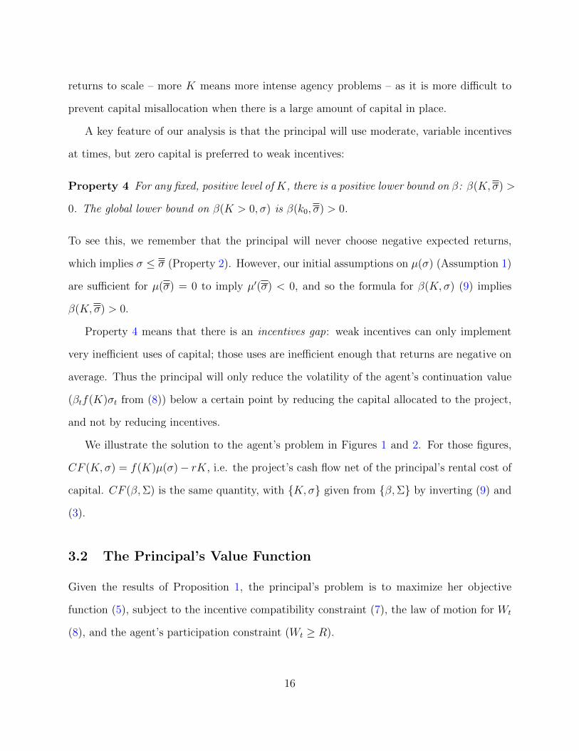
A key feature of our analysis is that the principal will use moderate, variable incentives

at times, but zero capital is preferred to weak incentives:

Property 4 For any fixed, positive level of K, there is a positive lower bound on β: β(K, σ) >

0. The global lower bound on β(K > 0, σ) is β(k0, σ) > 0.

To see this, we remember that the principal will never choose negative expected returns,

which implies σ ≤ σ (Property 2). However, our initial assumptions on µ(σ) (Assumption 1)

are sufficient for µ(σ) = 0 to imply µ′(σ) < 0, and so the formula for β(K, σ) (9) implies

β(K, σ) > 0.

Property 4 means that there is an incentives gap: weak incentives can only implement

very inefficient uses of capital; those uses are inefficient enough that returns are negative on

average. Thus the principal will only reduce the volatility of the agent’s continuation value

(βtf(K)σt from (8)) below a certain point by reducing the capital allocated to the project,

and not by reducing incentives.

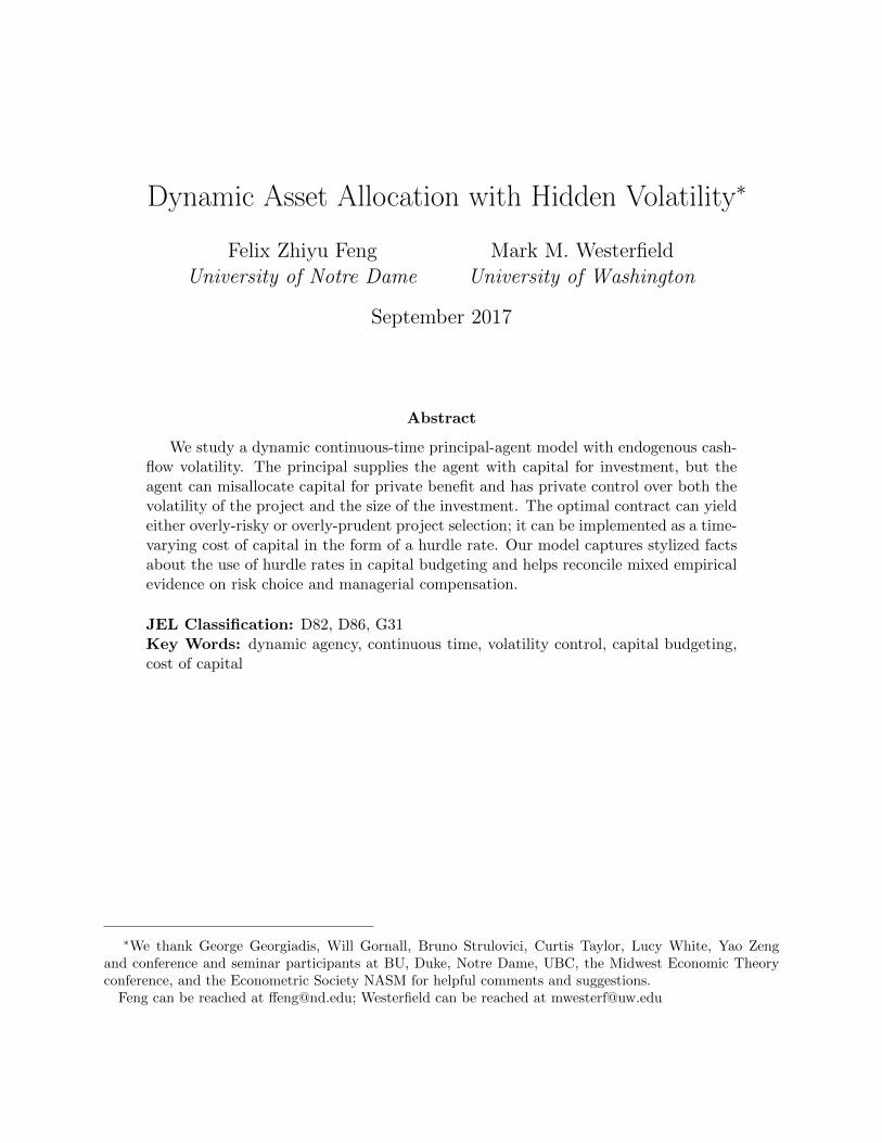
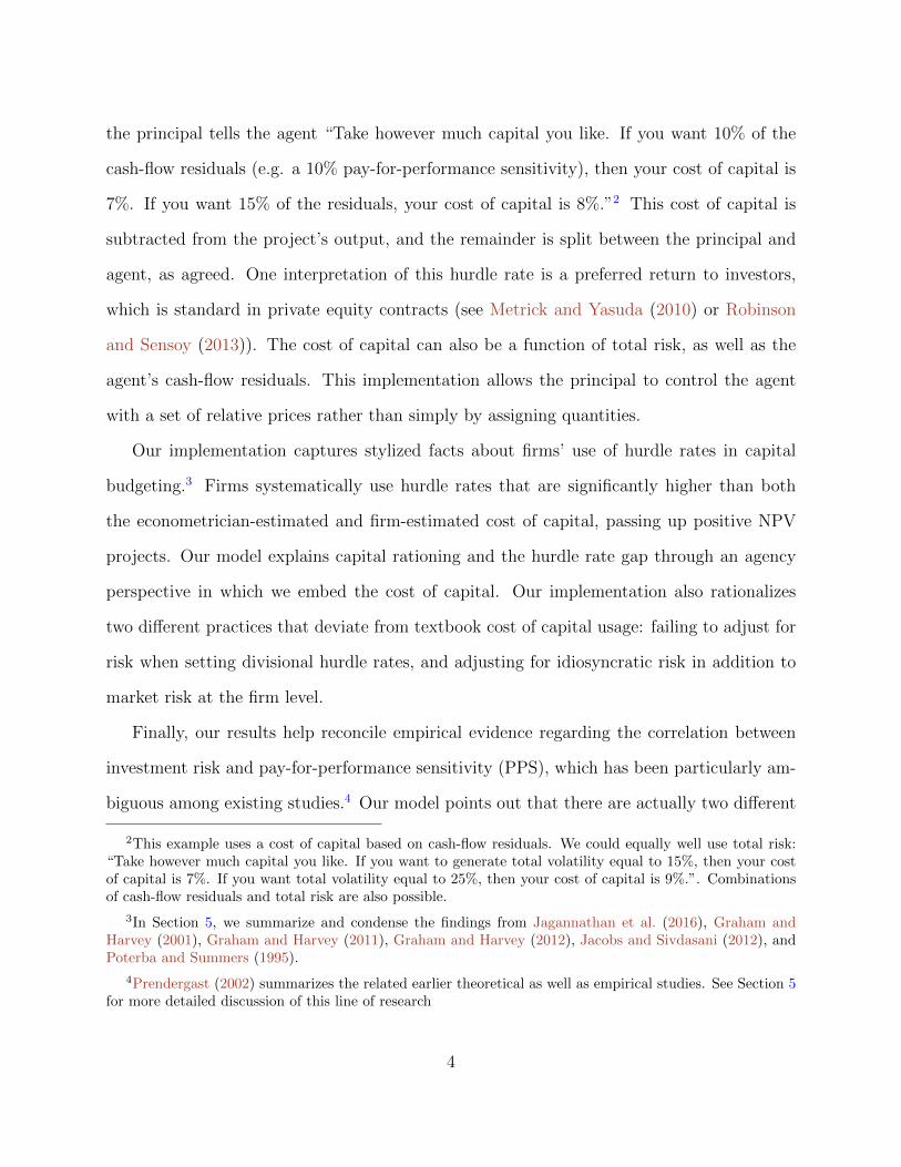
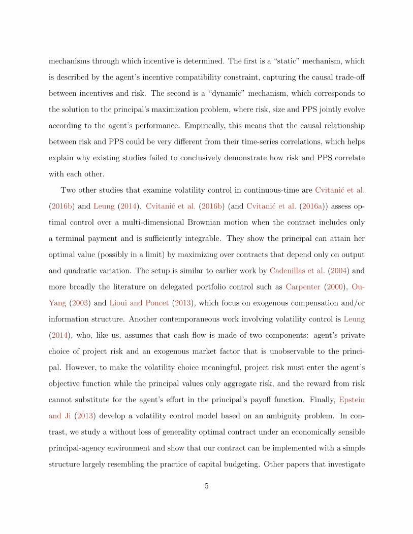
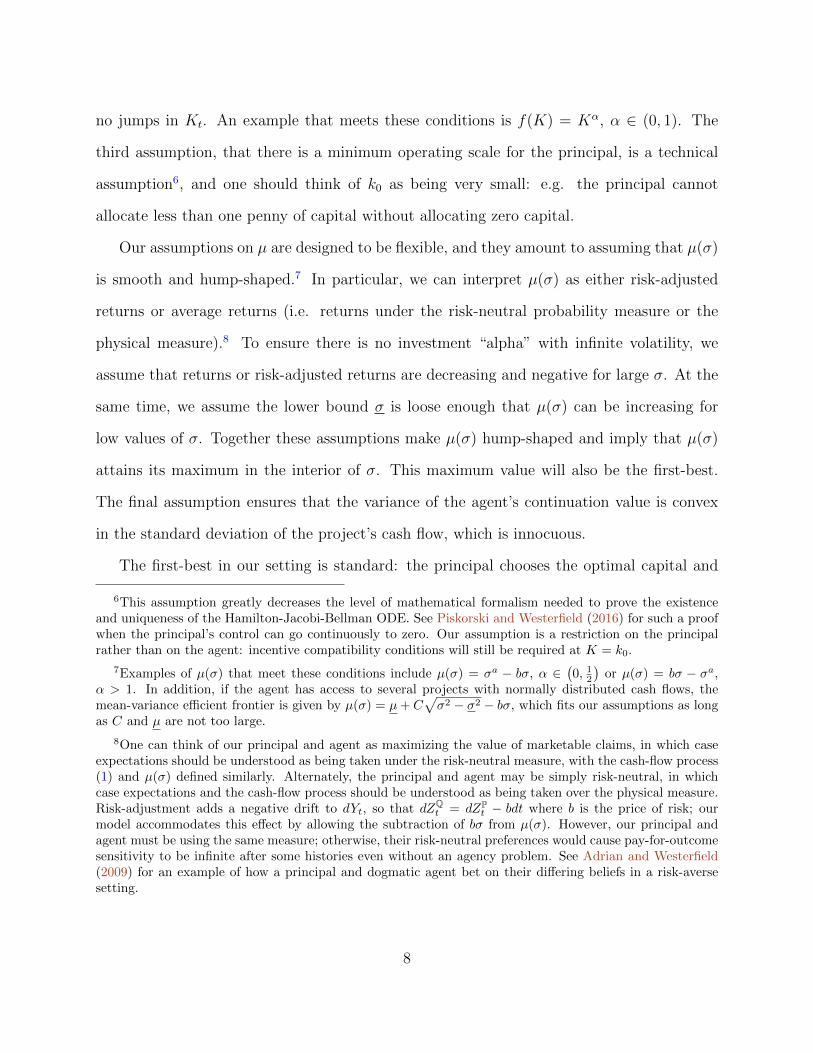
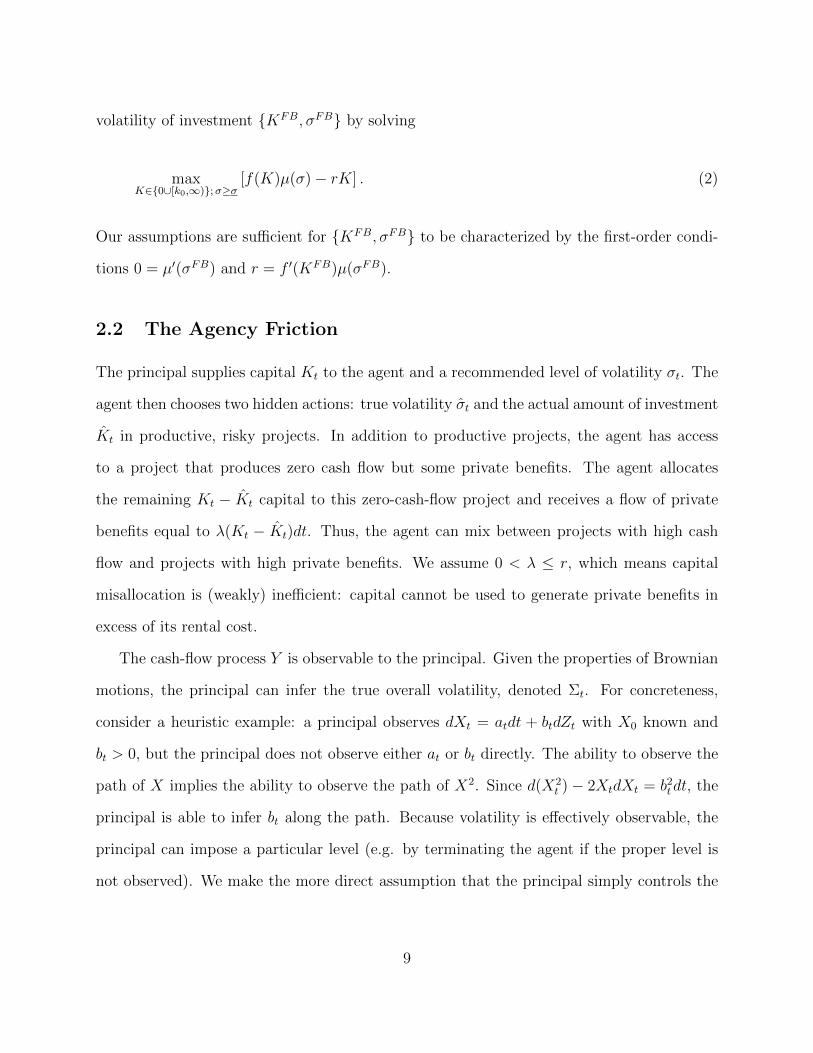
We illustrate the solution to the agent’s problem in Figures 1 and 2. For those figures,

CF (K, σ) = f(K)µ(σ)− rK, i.e. the project’s cash flow net of the principal’s rental cost of

capital. CF (β,Σ) is the same quantity, with K, σ given from β,Σ by inverting (9) and

(3).

3.2 The Principal’s Value Function

Given the results of Proposition 1, the principal’s problem is to maximize her objective

function (5), subject to the incentive compatibility constraint (7), the law of motion for Wt

(8), and the agent’s participation constraint (Wt ≥ R).

16

0.05 0.1 0.15 0.2<

0

0.5

1

-(<

,K)

0 2 4 6 8K

0

0.5

1

-(<

,K)

0.05 0.1 0.15 0.2<

0.15

0.2

0.25

0.3

CF

(<,K

)

0 2 4 6 8K

0

0.1

0.2

0.3

CF

(<,K

)

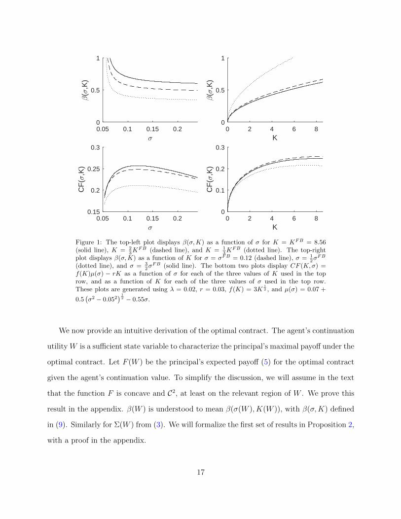
Figure 1: The top-left plot displays β(σ,K) as a function of σ for K = KFB = 8.56(solid line), K = 2

3KFB (dashed line), and K = 1

3KFB (dotted line). The top-right

plot displays β(σ,K) as a function of K for σ = σFB = 0.12 (dashed line), σ = 12σ

FB

(dotted line), and σ = 32σ

FB (solid line). The bottom two plots display CF (K,σ) =f(K)µ(σ) − rK as a function of σ for each of the three values of K used in the toprow, and as a function of K for each of the three values of σ used in the top row.These plots are generated using λ = 0.02, r = 0.03, f(K) = 3K

12 , and µ(σ) = 0.07 +

0.5(σ2 − 0.052

) 12 − 0.55σ.

We now provide an intuitive derivation of the optimal contract. The agent’s continuation

utility W is a sufficient state variable to characterize the principal’s maximal payoff under the

optimal contract. Let F (W ) be the principal’s expected payoff (5) for the optimal contract

given the agent’s continuation value. To simplify the discussion, we will assume in the text

that the function F is concave and C2, at least on the relevant region of W . We prove this

result in the appendix. β(W ) is understood to mean β(σ(W ), K(W )), with β(σ,K) defined

in (9). Similarly for Σ(W ) from (3). We will formalize the first set of results in Proposition 2,

with a proof in the appendix.

17

0 0.5 1-

0

2

4

6

8

K(-

,')

0 0.5 1-

0.05

0.1

0.15

0.2

<(-

,')

0 0.5 1-

0

0.1

0.2

0.3

CF

(-,'

)

0 0.5 1'

0

0.1

0.2

0.3

CF

(-,'

)

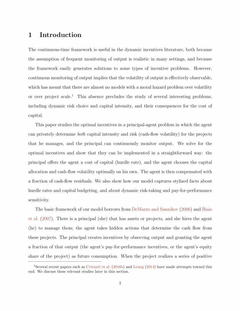
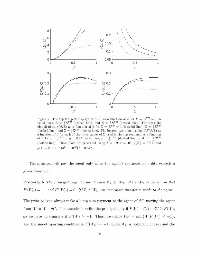
Figure 2: The top-left plot displays K(β,Σ) as a function of β for Σ = ΣFB = 1.05(solid line), Σ = 2

3ΣFB (dashed line), and Σ = 13ΣFB (dotted line). The top-right

plot displays σ(β,Σ) as a function of β for Σ = ΣFB = 1.05 (solid line), Σ = 23ΣFB

(dashed line), and Σ = 13ΣFB (dotted line). The bottom two plots display CF (β,Σ) as

a function of β for each of the three values of Σ used in the top row, and as a functionof Σ for β = βFB = λ

r = 0.67 (solid line), β = 23β

FB (dashed line), and β = 13β

FB

(dotted line). These plots are generated using λ = .02, r = .03, f(K) = 3K12 , and

µ(σ) = 0.07 + .5(σ2 − 0.052

) 12 − 0.55σ.

The principal will pay the agent only when the agent’s continuation utility exceeds a

given threshold:

Property 5 The principal pays the agent when Wt ≥ WC, where WC is chosen so that

F ′(WC) = −1 and F ′′(WC) = 0. If W0 > WC, an immediate transfer is made to the agent.

The principal can always make a lump-sum payment to the agent of dC, moving the agent

from W to W − dC. This transfer benefits the principal only if F (W − dC)− dC ≥ F (W ),

so we have no transfers if F ′(W ) ≥ −1. Thus, we define WC = minW |F ′(W ) ≤ −1,

and the smooth-pasting condition is F ′(WC) = −1. Since WC is optimally chosen and the

18

principal has linear utility, we have the super-contact condition F ′′(WC) = 0.12 This property

generates our first boundary condition, at the right boundary WC .

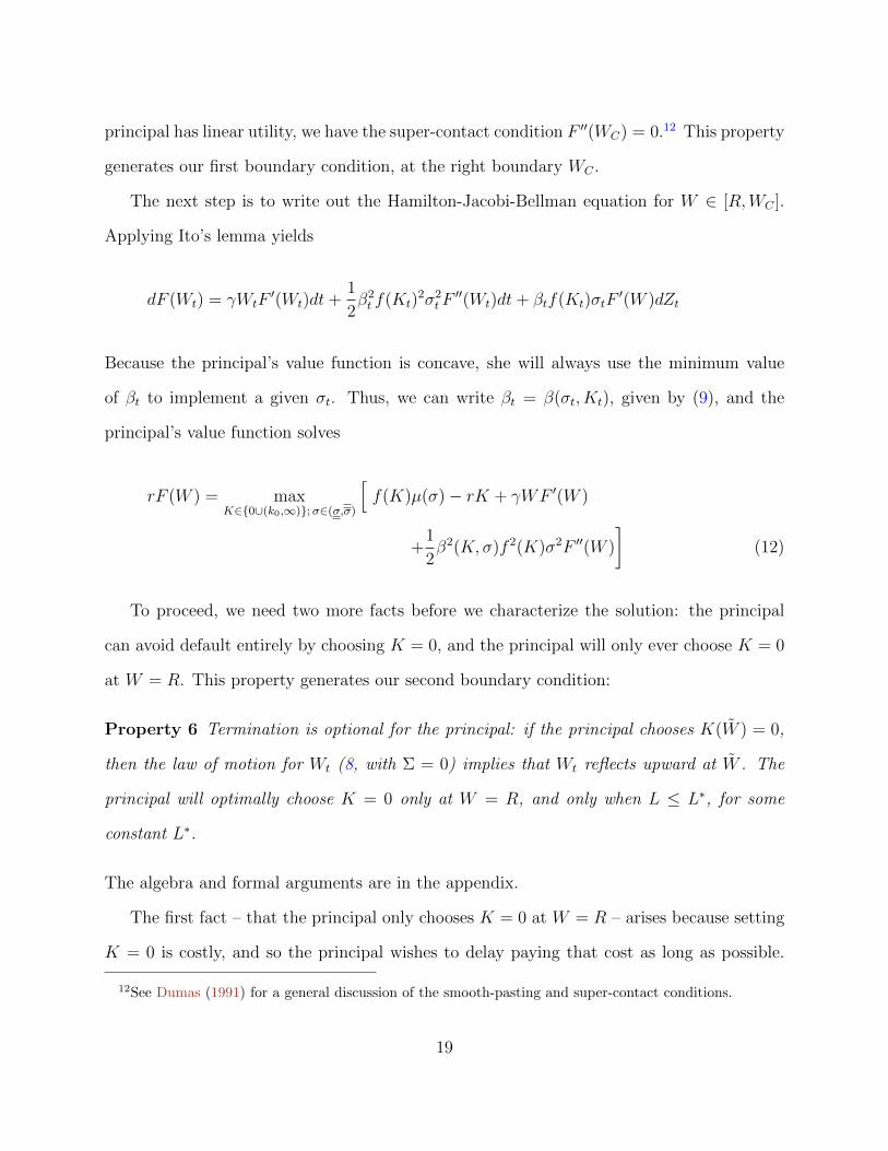
The next step is to write out the Hamilton-Jacobi-Bellman equation for W ∈ [R,WC ].

Applying Ito’s lemma yields

dF (Wt) = γWtF′(Wt)dt+

1

2β2t f(Kt)

2σ2tF′′(Wt)dt+ βtf(Kt)σtF

′(W )dZt

Because the principal’s value function is concave, she will always use the minimum value

of βt to implement a given σt. Thus, we can write βt = β(σt, Kt), given by (9), and the

principal’s value function solves

rF (W ) = maxK∈0∪(k0,∞);σ∈(σ,σ)

[f(K)µ(σ)− rK + γWF ′(W )

+1

2β2(K, σ)f 2(K)σ2F ′′(W )

](12)

To proceed, we need two more facts before we characterize the solution: the principal

can avoid default entirely by choosing K = 0, and the principal will only ever choose K = 0

at W = R. This property generates our second boundary condition:

Property 6 Termination is optional for the principal: if the principal chooses K(W ) = 0,

then the law of motion for Wt (8, with Σ = 0) implies that Wt reflects upward at W . The

principal will optimally choose K = 0 only at W = R, and only when L ≤ L∗, for some

constant L∗.

The algebra and formal arguments are in the appendix.

The first fact – that the principal only chooses K = 0 at W = R – arises because setting

K = 0 is costly, and so the principal wishes to delay paying that cost as long as possible.

12See Dumas (1991) for a general discussion of the smooth-pasting and super-contact conditions.

19

There are two costs to setting K = 0. One is an opportunity cost because any time with

K = 0 is time the principal might otherwise have positive expected cash flow. The second

cost is that by causing Wt to reflect early, the principal is causing Wt to reflect upward at

a level that is closer to the agent’s consumption boundary, so the agent will be awarded

consumption sooner. The second fact is that the principal only chooses K = 0 if L is low.

This is economically very clear: the principal only avoids default and termination if her value

in default is low. If L is high enough, the principal simply accepts default rather than pay

the costs associated with K = 0.

The principal’s value function is concave because of the costs associated with termination,

even if termination does not occur in equilibrium. If L > L∗, there is a direct cost associated

with termination as long as L is less than the discounted, first-best cash flow. This cost

makes volatility undesirable, and the principal’s value function is concave. If L < L∗, there

is a direct cost to termination that the principal avoids in equilibrium, choosing instead to

pay the opportunity cost of shutting down the project. The principal forgoes the project’s

cash flow, allowing the agent’s continuation value to reflect upwards.

We formalize our derivation as follows:

Proposition 2 A solution to the principal’s problem exists, is unique, is concave on W ∈

[R,WC ], has F ′(WC) = −1 and F ′′(WC) = 0, solves (12), is C for all W and C3 for all

W ∈ (R,WC), and has F (R) = L > L∗ if K(R) > 0 and F (R) = L∗ if K(R) = 0. The

agent’s continuation utility evolves as in (8), which has a unique weak solution.

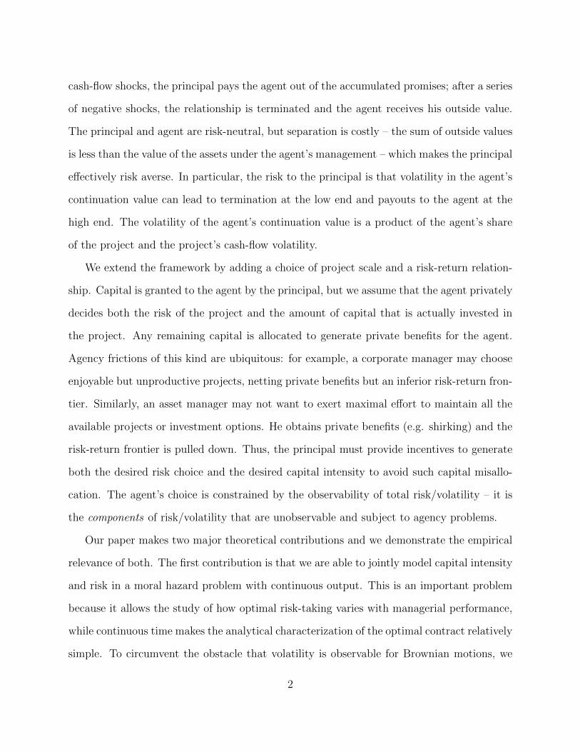
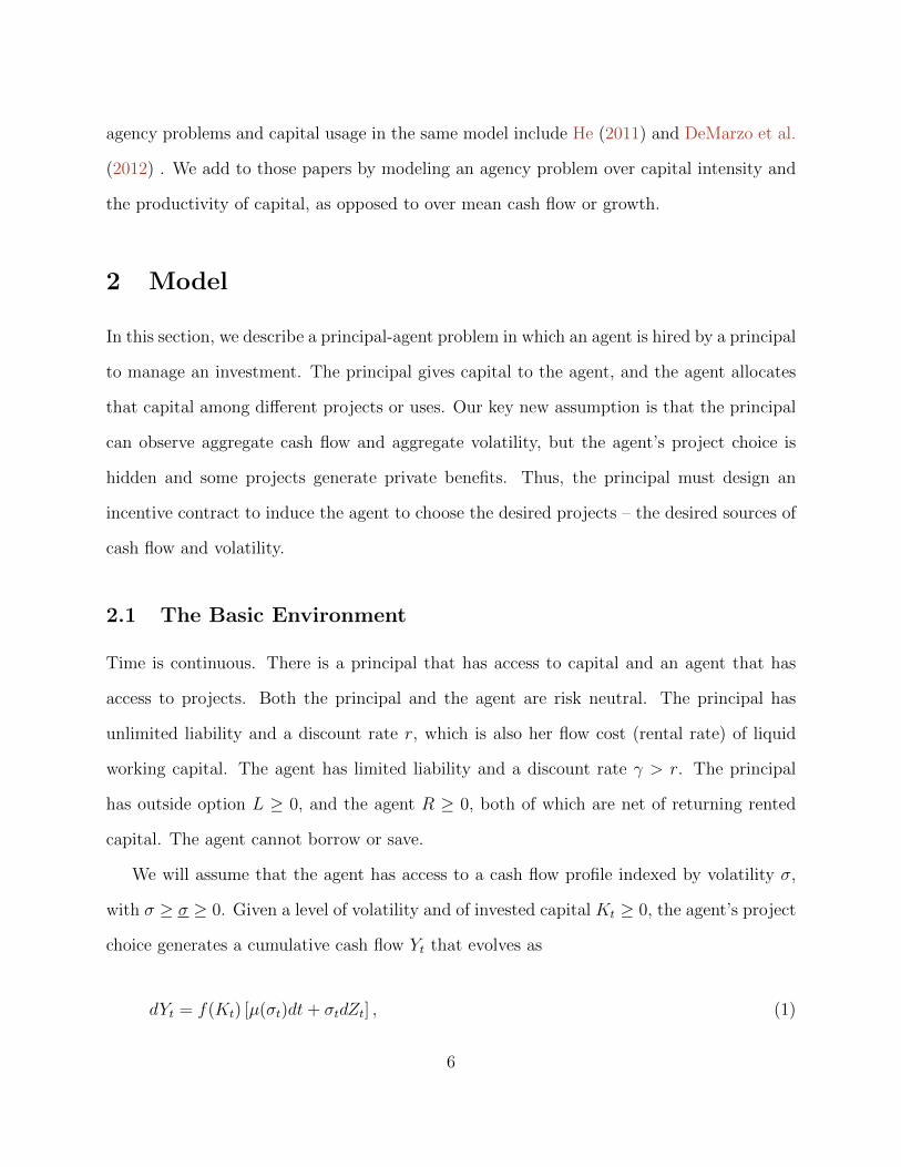
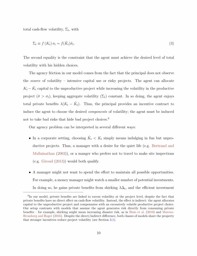
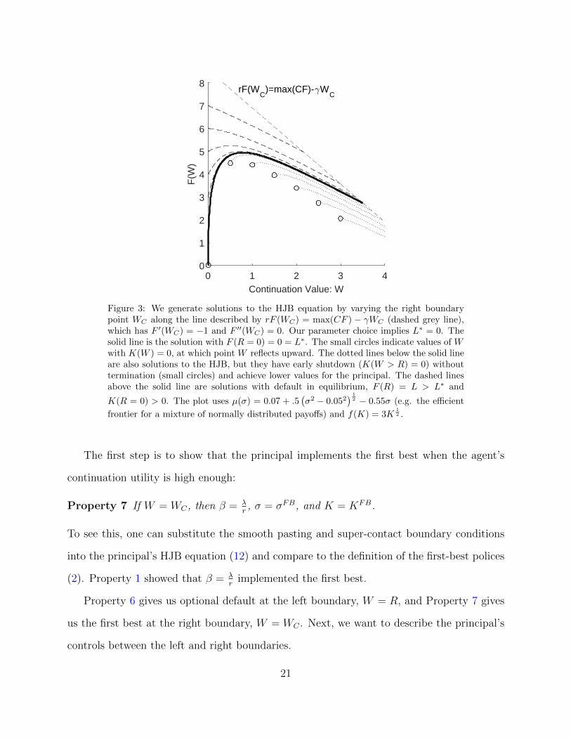
We illustrate our construction in Figure 3.

3.3 Contract Description

We have characterized the solution as an ODE with boundary conditions. Now, we describe

the properties of the optimal contract and some comparative statics.

20

0 1 2 3 4Continuation Value: W

0

1

2

3

4

5

6

7

8

F(W

)

rF(WC

)=max(CF)-.WC

Figure 3: We generate solutions to the HJB equation by varying the right boundarypoint WC along the line described by rF (WC) = max(CF ) − γWC (dashed grey line),which has F ′(WC) = −1 and F ′′(WC) = 0. Our parameter choice implies L∗ = 0. Thesolid line is the solution with F (R = 0) = 0 = L∗. The small circles indicate values of Wwith K(W ) = 0, at which point W reflects upward. The dotted lines below the solid lineare also solutions to the HJB, but they have early shutdown (K(W > R) = 0) withouttermination (small circles) and achieve lower values for the principal. The dashed linesabove the solid line are solutions with default in equilibrium, F (R) = L > L∗ and

K(R = 0) > 0. The plot uses µ(σ) = 0.07 + .5(σ2 − 0.052

) 12 − 0.55σ (e.g. the efficient

frontier for a mixture of normally distributed payoffs) and f(K) = 3K12 .

The first step is to show that the principal implements the first best when the agent’s

continuation utility is high enough:

Property 7 If W = WC, then β = λr, σ = σFB, and K = KFB.

To see this, one can substitute the smooth pasting and super-contact boundary conditions

into the principal’s HJB equation (12) and compare to the definition of the first-best polices

(2). Property 1 showed that β = λr

implemented the first best.

Property 6 gives us optional default at the left boundary, W = R, and Property 7 gives

us the first best at the right boundary, W = WC . Next, we want to describe the principal’s

controls between the left and right boundaries.

21

There are two useful ways of understanding the principal’s choices. The first is to examine

the cash-flow inputs, K, σ. These give us capital and risk choices at the investment level.

The second is to examine the principal’s volatility controls, Σ, β. These give us volatility

and incentive choices at the relationship level. The mapping between K, σ and Σ, β is

given by the formulas for Σ and β (3 and 9).

To proceed, we first define, with a slight abuse of notation,

E [dY − rKdt] = CF (K, σ) = CF (Σ, β) (13)

g(K) = λf(K)

f ′(K)(14)

h(σ) =σ

µ(σ)− σµ′(σ)(15)

Then, we can write the HJB equation (12) as

rF (W ) = maxK,σ

[CF (K, σ) + γWF ′(W ) +

1

2g(K)2h(σ)2F ′′(W )

](16)

rF (W ) = maxΣ, β

[CF (Σ, β) + γWF ′(W ) +

1

2Σ2β2F ′′(W )

](17)

Our model produces some easy comparative statics. Since the first best is achieved

at WC with F ′′(WC) = 0, the revised HJB equations (16 and 17) show that first-best is

characterized by CFK(K, σ) = CFσ(K, σ) = CFΣ(Σ, β) = CFβ(Σ, β) = 0. Assumption 1

implies that g′(K) > 0, and that we can use the first-order conditions to characterize the

choices of K, σ and Σ, β. Direct calculation yields

Property 8 The principal chooses Σt ≤ ΣFB, βt ≤ βFB, and Kt ≤ KFB.

If h′(σ) > 0, the principal chooses σt ≤ σFB. If h′(σ) < 0, then the principal chooses

σt ≥ σFB.

The inequalities are strict for W < WC, and follow from F ′′ < 0.

22

This property shows that the agency friction always causes the principal to reduce in-

centives below the level that would induce the first-best policies (βt ≤ βFB), and to do so in

a way that reduces cash-flow volatility (Σt ≤ ΣFB). This is not a-priori obvious: the source

of risk for the principal is volatility in the agent’s continuation value, which can lead to a

loss in default or near-default. Importantly, this risk is driven by the volatility of the agent’s

continuation value, not the volatility of the project’s cash flow. The volatility of the agent’s

continuation value is the product Σβ, and so one can imagine that the principal might reduce

the agent’s share of volatility, imposing weaker incentives and allowing for more volatile cash

flow. However, both Σ and β increase the expected cash flow, and they are complements in

the cost term (12β2Σ2F ′′(W )), so the principal reduces them both. This is not the case with

project-level volatility, as we now describe.

Property 8 shows that the optimal contract may implement levels of project-based risk (σ)

that are higher or lower than the first-best. The reason is that σ affects the volatility of the

agent’s continuation value through two opposing mechanisms: on the one hand, Property 3

shows that βσ < 0. That is, implementing a smaller σ (which leads to a more risk-efficient

cash flow) requires stronger incentives. On the other hand, cash-flow volatility is increasing

in project-level volatility since Σ = f(K)σ. The volatility of the agent’s continuation value

is a product of these two effects, Σσ > 0 and βσ < 0, so whether the optimal contract

implements a higher or lower σ relative to the first-best depends on which effect dominates.

The function h(σ) captures the effect of σ on continuation value volatility (Σβ = g(K)h(σ)).

When h′(σ) > 0, this means that higher project-level volatility implies higher continuation-

value volatility, and the principal reduces risk by reducing both volatilities – implementing σ

that is lower than the first-best. When h′(σ) < 0, higher project-level volatility implies lower

continuation-value volatility, and the principal reduces her risk by offering weak incentives

– implementing σ that is higher than the first-best. The critical distinction here is between

cash-flow volatility and continuation-value volatility. The agency problem dictates that it is

23

the risk of default and termination that generates losses – and therefor the agent’s continu-

ation value volatility that generates risk – but risky projects can be implemented by giving

the agent a small share of those projects, and this creates low continuation-value volatility.

In contrast, while capital K also affects the size of the agency problem through the same

two channels, it does so in the same direction because βK and ΣK are both positive. Thus

the optimal contract always features under-investment (Kt ≤ KFB) relative to the first best.

We can also assess the marginal rate of technical substitution between project inputs

(K, σ) and between the principal’s incentive tools (Σ, β). Combining the first-order

conditions to eliminate the F ′′ term yields

Property 9 For W such that K > k0, we have

CFK(K, σ)

CFσ(K, σ)=g′(K)h(σ)

g(K)h′(σ)(18)

and

∂CF (Σ, β)

∂ ln Σ=∂CF (Σ, β)

∂ ln β= −Σ2β2F ′′(W ) ≥ 0 (19)

The inequality in (19) is strict for W < WC, and follows from F ′′(W ) < 0.

The first equation (18) shows that the principal sets the marginal rate of technical substitu-

tion between K and σ for cash flow (CF (K, σ)) equal to that for volatility (g(K)h(σ)). This

is the direct tradeoff between capital intensity and project choice: volatility in the agent’s

continuation value (i.e. volatility that leads to default) is the cost of positive cash flow, and

so the principal equalizes the marginal values of K and σ.

The second equation (19) gives another view of the principal’s optimization problem.

The principal has two volatility controls: aggregate cash-flow volatility (Σ), and the fraction

of that volatility carried by the agent (β). We see that the principal maintains equality in

24

logs for the marginal products of these choice variables. For example, a 10% increase in

aggregate volatility and a 10% increase in the agent’s share will, in equilibrium, have equal

effects on expected cash flow. Then, both Σt and βt are reduced – their marginal product

increased – when the principal is effectively more risk averse.

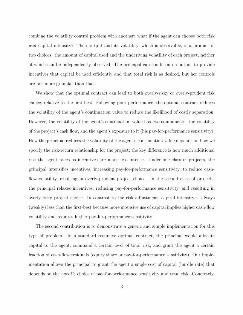
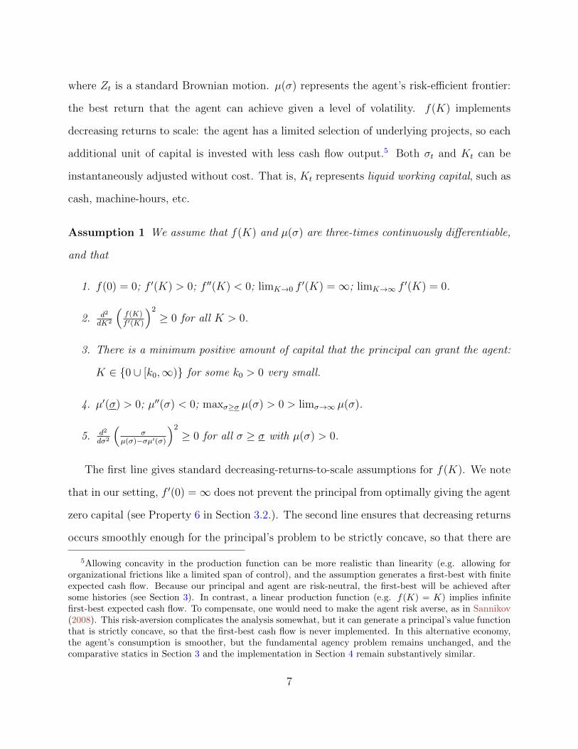
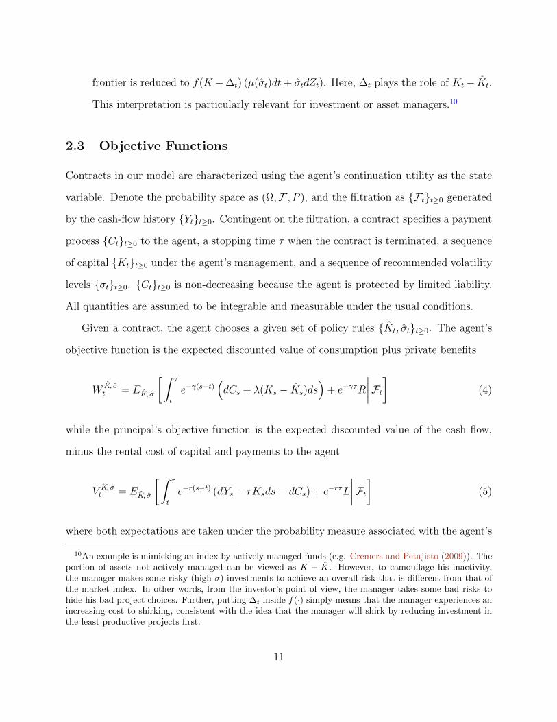
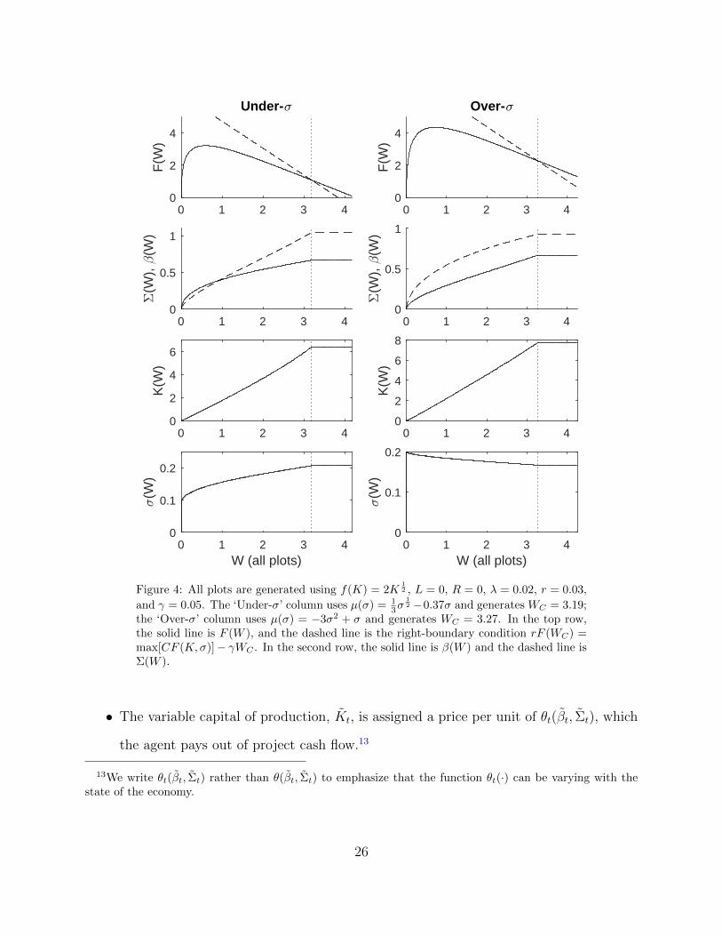
We illustrate an optimal contract in Figure 4. We label solutions for h′(σ) > 0 and

σt ≤ σFB as “Under-σ”; solutions for h′(σ) < 0 and σt ≥ σFB are “Over-σ”.

Finally, we note that the optimal contract is robust to considering positive capital mis-

allocation in equilibrium:

Property 10 If we generalize Definition 1 to allow for capital misallocation (private ben-

efits) in optimal contracts, then all optimal contracts implement zero misallocation, except

possibly at WC.

The proof is in the appendix. The intuition is that misallocation is assumed to be weakly

inefficient (λ ≤ r).

4 Implementation

In this section, we show that the optimal contract can be implemented with a startlingly

simple structure: the principal assigns the project a hurdle rate, against which to measure

agent performance, and the agent chooses everything else (capital obtained from the princi-

pal, capital actually invested, project risk, and pay-for-performance sensitivity). Of course,

the principal can restrict the agent’s choice to a subset of those variables as well.

In its most basic form, the principal offers to rent capital to the agent as follows:

• The fixed capital of production (the assets that have liquidation value L) is assigned

a price φt that the agent pays out of his continuation value (e.g. in forgone future

consumption).

25

0 1 2 3 40

2

4

F(W

)

Under-<

0 1 2 3 40

0.5

1

'(W

), -

(W)

0 1 2 3 40

2

4

6

K(W

)

0 1 2 3 4W (all plots)

0

0.1

0.2

<(W

)

0 1 2 3 40

2

4

F(W

)

Over-<

0 1 2 3 40

0.5

1

'(W

), -

(W)

0 1 2 3 40

2

4

6

8

K(W

)

0 1 2 3 4W (all plots)

0

0.1

0.2

<(W

)

Figure 4: All plots are generated using f(K) = 2K12 , L = 0, R = 0, λ = 0.02, r = 0.03,

and γ = 0.05. The ‘Under-σ’ column uses µ(σ) = 13σ

12 −0.37σ and generates WC = 3.19;

the ‘Over-σ’ column uses µ(σ) = −3σ2 + σ and generates WC = 3.27. In the top row,the solid line is F (W ), and the dashed line is the right-boundary condition rF (WC) =max[CF (K,σ)]− γWC . In the second row, the solid line is β(W ) and the dashed line isΣ(W ).

• The variable capital of production, Kt, is assigned a price per unit of θt(βt, Σt), which

the agent pays out of project cash flow.13

13We write θt(βt, Σt) rather than θ(βt, Σt) to emphasize that the function θt(·) can be varying with thestate of the economy.

26

• The agent chooses Kt, βt, Σt. The tilde notation is used to indicate that those quan-

tities are choices of the agent. The agent then chooses Kt, σt (capital allocated

to productive projects and the associated volatility, as in the standard problem) to

generate cash flow dYt.

The net project cash flow is

dY NEWt ≡ dYt − Ktθt(βt, Σt)dt, (20)

with φtdt taken directly from the agent’s continuation value. The agent receives a βt fraction

of net project cash flow. This implies that the project’s cash flow bears the full cost of capital

while the agent bears a fraction β. Thus, in addition to a more abstract incentive device, we

can interpret the hurdle rate as a preferred return to investors, which is standard in private

equity contracts (see Metrick and Yasuda (2010) or Robinson and Sensoy (2013)).

This setup allows the agent to choose his own equity share, the cash-flow volatility, and

the capital quantity used. The principal only offers a (time-varying) cost of capital that is

adjusted if the agent announces he will take a different cash-flow residual (β) or generate

undesired volatility (Σ). In addition, the principal imposes the constraint that the agent

must choose the set β, K, Σ to be either all strictly positive or all zero. To induce the

agent to choose β = 0, K = 0, Σ = 0, the principal offers φ, θ = 0,∞.

The adjusted cash-flow technology (20) does not change the basic information asym-

metry problem because the adjustment is observable to both sides. The agent’s choices of

Kt, βt, Σt are observable to the principal, even without the cost of capital mechanism: β

because the principal can always observe the cash-flow residual she pays to the agent, Kt

because the principal can observe the capital she turns over to the agent, and Σt from the

quadratic variation in dYt.14

14To avoid any technical issues, we will simply assume that the agent commits to using the value of Σ

27

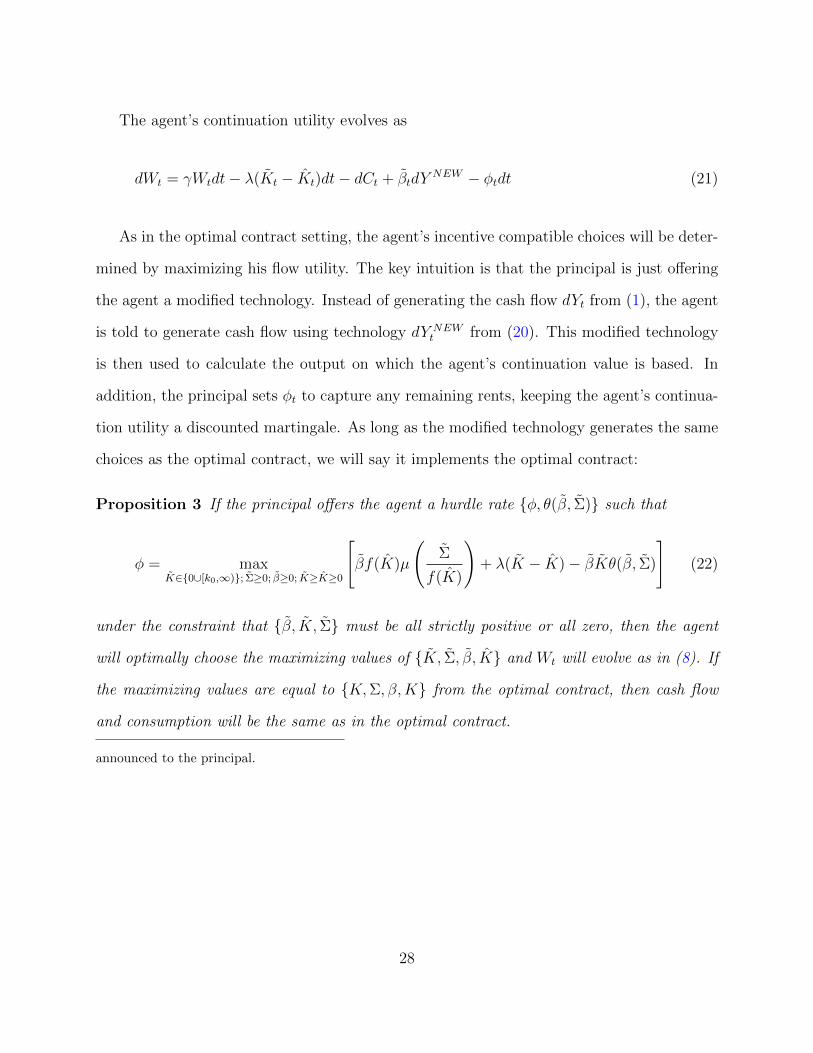
The agent’s continuation utility evolves as

dWt = γWtdt− λ(Kt − Kt)dt− dCt + βtdYNEW − φtdt (21)

As in the optimal contract setting, the agent’s incentive compatible choices will be deter-

mined by maximizing his flow utility. The key intuition is that the principal is just offering

the agent a modified technology. Instead of generating the cash flow dYt from (1), the agent

is told to generate cash flow using technology dY NEWt from (20). This modified technology

is then used to calculate the output on which the agent’s continuation value is based. In

addition, the principal sets φt to capture any remaining rents, keeping the agent’s continua-

tion utility a discounted martingale. As long as the modified technology generates the same

choices as the optimal contract, we will say it implements the optimal contract:

Proposition 3 If the principal offers the agent a hurdle rate φ, θ(β, Σ) such that

φ = maxK∈0∪[k0,∞); Σ≥0; β≥0; K≥K≥0

[βf(K)µ

(Σ

f(K)

)+ λ(K − K)− βKθ(β, Σ)

](22)

under the constraint that β, K, Σ must be all strictly positive or all zero, then the agent

will optimally choose the maximizing values of K, Σ, β, K and Wt will evolve as in (8). If

the maximizing values are equal to K,Σ, β,K from the optimal contract, then cash flow

and consumption will be the same as in the optimal contract.

announced to the principal.

28

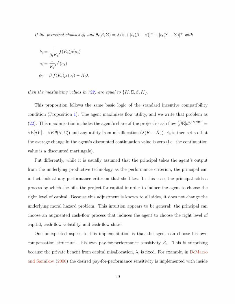
If the principal chooses φt and θt(β, Σ) = λ/β + [bt(β − β)]+ + [ct(Σ− Σ)]+ with

bt =1

βtKt

f(Kt)µ(σt)

ct =1

Kt

µ′ (σt)

φt = βtf(Kt)µ (σt)−Ktλ

then the maximizing values in (22) are equal to K,Σ, β,K.

This proposition follows the same basic logic of the standard incentive compatibility

condition (Proposition 1). The agent maximizes flow utility, and we write that problem as

(22). This maximization includes the agent’s share of the project’s cash flow (βE[dY NEW ] =

βE[dY ]− βKθ(β, Σ)) and any utility from misallocation (λ(K − K)). φt is then set so that

the average change in the agent’s discounted continuation value is zero (i.e. the continuation

value is a discounted martingale).

Put differently, while it is usually assumed that the principal takes the agent’s output

from the underlying productive technology as the performance criterion, the principal can

in fact look at any performance criterion that she likes. In this case, the principal adds a

process by which she bills the project for capital in order to induce the agent to choose the

right level of capital. Because this adjustment is known to all sides, it does not change the

underlying moral hazard problem. This intuition appears to be general: the principal can

choose an augmented cash-flow process that induces the agent to choose the right level of

capital, cash-flow volatility, and cash-flow share.

One unexpected aspect to this implementation is that the agent can choose his own

compensation structure – his own pay-for-performance sensitivity βt. This is surprising

because the private benefit from capital misallocation, λ, is fixed. For example, in DeMarzo

and Sannikov (2006) the desired pay-for-performance sensitivity is implemented with inside

29

equity that is chosen so that the marginal benefit from reporting additional cash flow is

equal to the marginal benefit from capital misallocation. Both are constant. Instead, our

model works by having the agent trade off two different controls, βt and Kt. If βt is chosen

to be very small, the cost of capital will be very high, and so the agent has to use the capital

productively to avoid a loss of continuation value. If βt is chosen to be high, then capital

is cheap, but the gains to capital misallocation are lower than the agent’s chosen cash-flow

residual (pay-for-performance sensitivity).

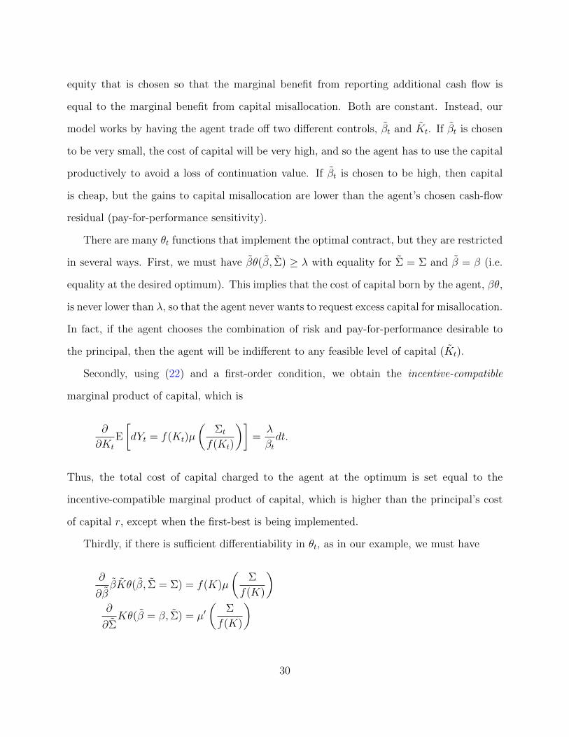
There are many θt functions that implement the optimal contract, but they are restricted

in several ways. First, we must have βθ(β, Σ) ≥ λ with equality for Σ = Σ and β = β (i.e.

equality at the desired optimum). This implies that the cost of capital born by the agent, βθ,

is never lower than λ, so that the agent never wants to request excess capital for misallocation.

In fact, if the agent chooses the combination of risk and pay-for-performance desirable to

the principal, then the agent will be indifferent to any feasible level of capital (Kt).

Secondly, using (22) and a first-order condition, we obtain the incentive-compatible

marginal product of capital, which is

∂

∂Kt

E

[dYt = f(Kt)µ

(Σt

f(Kt)

)]=

λ

βtdt.

Thus, the total cost of capital charged to the agent at the optimum is set equal to the

incentive-compatible marginal product of capital, which is higher than the principal’s cost

of capital r, except when the first-best is being implemented.

Thirdly, if there is sufficient differentiability in θt, as in our example, we must have

∂

∂ββKθ(β, Σ = Σ) = f(K)µ

(Σ

f(K)

)∂

∂ΣKθ(β = β, Σ) = µ′

(Σ

f(K)

)

30

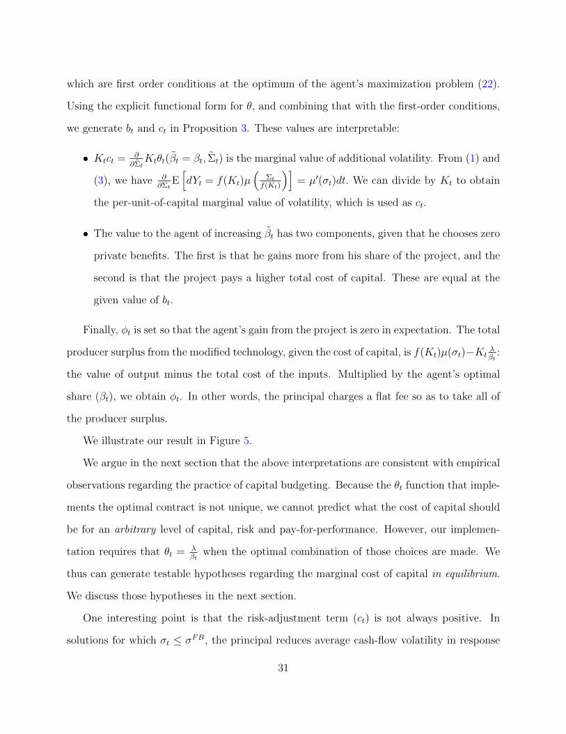
which are first order conditions at the optimum of the agent’s maximization problem (22).

Using the explicit functional form for θ, and combining that with the first-order conditions,

we generate bt and ct in Proposition 3. These values are interpretable:

• Ktct = ∂∂Σt

Ktθt(βt = βt, Σt) is the marginal value of additional volatility. From (1) and

(3), we have ∂∂Σt

E[dYt = f(Kt)µ

(Σt

f(Kt)

)]= µ′(σt)dt. We can divide by Kt to obtain

the per-unit-of-capital marginal value of volatility, which is used as ct.

• The value to the agent of increasing βt has two components, given that he chooses zero

private benefits. The first is that he gains more from his share of the project, and the

second is that the project pays a higher total cost of capital. These are equal at the

given value of bt.

Finally, φt is set so that the agent’s gain from the project is zero in expectation. The total

producer surplus from the modified technology, given the cost of capital, is f(Kt)µ(σt)−Ktλβt

:

the value of output minus the total cost of the inputs. Multiplied by the agent’s optimal

share (βt), we obtain φt. In other words, the principal charges a flat fee so as to take all of

the producer surplus.

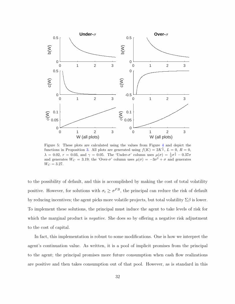
We illustrate our result in Figure 5.

We argue in the next section that the above interpretations are consistent with empirical

observations regarding the practice of capital budgeting. Because the θt function that imple-

ments the optimal contract is not unique, we cannot predict what the cost of capital should

be for an arbitrary level of capital, risk and pay-for-performance. However, our implemen-

tation requires that θt = λβt

when the optimal combination of those choices are made. We

thus can generate testable hypotheses regarding the marginal cost of capital in equilibrium.

We discuss those hypotheses in the next section.

One interesting point is that the risk-adjustment term (ct) is not always positive. In

solutions for which σt ≤ σFB, the principal reduces average cash-flow volatility in response

31

0 1 2 30

0.5

b(W

)

Under-<

0 1 2 30

0.5

c(W

)

0 1 2 3W (all plots)

0

0.05

0.1

?(W

)

0 1 2 30

0.5

b(W

)

Over-<

0 1 2 3-0.5

0

c(W

)

0 1 2 3W (all plots)

0

0.05

0.1

?(W

)

Figure 5: These plots are calculated using the values from Figure 4 and depict thefunctions in Proposition 3. All plots are generated using f(K) = 2K

12 , L = 0, R = 0,

λ = 0.02, r = 0.03, and γ = 0.05. The ‘Under-σ’ column uses µ(σ) = 13σ

12 − 0.37σ

and generates WC = 3.19; the ‘Over-σ’ column uses µ(σ) = −3σ2 + σ and generatesWC = 3.27.

to the possibility of default, and this is accomplished by making the cost of total volatility

positive. However, for solutions with σt ≥ σFB, the principal can reduce the risk of default

by reducing incentives; the agent picks more volatile projects, but total volatility Σβ is lower.

To implement these solutions, the principal must induce the agent to take levels of risk for

which the marginal product is negative. She does so by offering a negative risk adjustment

to the cost of capital.

In fact, this implementation is robust to some modifications. One is how we interpret the

agent’s continuation value. As written, it is a pool of implicit promises from the principal

to the agent; the principal promises more future consumption when cash flow realizations

are positive and then takes consumption out of that pool. However, as is standard in this

32

type of model, the pool of implicit promises can be made into an explicit account (e.g. a

line of credit in DeMarzo and Sannikov (2006) or a cash balance in Biais et al. (2007)). Let

Mt be the balance on an account in the agent’s name, and assume that the agent’s cash-flow

residuals from the projects are paid into the account, the agent’s consumption is withdrawn

from the account, the agent pays φt−γR to the principal for the right to operate the project,

and that the account pays an interest rate of γ. Then we have

dMt = γMt + βtdYNEWt − (φt − γR) dt− dCt (23)

It is the case that Wt = Mt + R, so the agent consumes at Mt = WC − R and termination

occurs if L < L∗ and Mt = 0.15 A dynamic programming verification theorem is sufficient

to show that such an account will implement the optimal contract.

Finally, we have written the implementation so that the cost of variable capital (θt) is

deducted from the project cash flow instead of the continuation value. This is not required;

we could deduct the cost of variable capital from the cash or the line of credit directly. The

only difference is whether we interpret the cost of capital as being paid by the agent or by the

project (e.g. a preferred return to outside investors, or not). We can also take either βt or Σt

out of the agent’s choice set; i.e. we have presented the most decentralized implementation

by giving the agent the choice over both βt and Σt as well as Kt, but that is not required.

15If one wants the account to pay interest r, then, with this configuration, the agent pays the principalφt − γR − (γ − r)Mt for the right to operate the project. In addition, since the agent is indifferent to thetiming of his own consumption (as in DeMarzo and Sannikov (2006) and Biais et al. (2007)), we can assumethat the agent chooses consumption at the principal’s desired time.

33

5 Empirical Discussion

5.1 Capital Budgeting and the Cost of Capital

There is broad empirical agreement on the basic stylized facts surrounding the use of hurdle

rates for capital budgeting16:

• Most or almost all firms use DCF methods with a hurdle rate. That hurdle rate

is substantially above both the econometrician-estimated and firm-estimated cost of

capital. For example, Jagannathan et al. (2016) find an average hurdle rate of 15%

compared to an average cost of capital of 8%. They find that this is not likely to be

caused by behavioral biases or driven by managerial exaggeration.

• Firms engage in deliberate capital rationing. This rationing is often a response to

non-financial constraints; more that half of firms report that they pass up apparently

positive NPV projects because of constraints on managerial time and expertise (55.3%,

Jagannathan et al. (2016)).

• Most firms use a company-wide hurdle rate. Only 15% of the firms use divisional

hurdle rates (Graham and Harvey (2001)).

• About as many firms adjust for idiosyncratic risk as for market risk (65.4% versus

63.4%, Jagannathan et al. (2016)).

Our model is consistent with these results on hurdle rates and capital rationing: the

principal chooses a hurdle rate that is higher than the firm’s cost of capital, and this is

optimal because the agency problem imposes a constraint on the use of managerial time

and expertise. The principal must offer the agent a portion of residual cash flow in order

16This list is a summary of results in Jagannathan et al. (2016), Graham and Harvey (2001), Graham andHarvey (2011), Graham and Harvey (2012), Jacobs and Sivdasani (2012), and Poterba and Summers (1995).

34

to induce the desired project choice and capital usage. This portion, combined with limited

liability on the part of the manager, creates the possibility of termination, which entails the

loss of a high NPV project. To avoid the larger loss, the principal accepts the smaller loss of

reducing the scale of the agent’s activity, reducing the volatility of the agent’s residual claim.

In short, our model suggests that extracting the full value of the “time and expertise” of

managers is an agency problem that requires the principal to reduce the scale of the agent’s

production or investment activity. The mechanism by which the principal reduces the scale

of the agent’s activity is a capital rationing, created by a high hurdle rate.

Moreover, our model is consistent with firms using company-wide rather than divisional

hurdle rates, and with firms adjusting for idiosyncratic risk in addition to market risk.

Our model contains two risk adjustments, one explicit and one implicit. The explicit risk

adjustment applies to total risk: the hurdle rate is adjusted by the agent’s choice of Σ. The

purpose of capital rationing in our model is to reduce the agent’s exposure to volatility. The

level of incremental capital rationing due to total risk (ct) varies with manager’s performance,

but it is usually small. Recall that ct = 1Ktµ′(σ), and that Kt can be a large number while

µ′(σ) comes from a first-order condition and is usually near zero. In fact, risk adjustment

is strictly zero at the first-best (since µ′(σFB) = 0), and it is only large near default (when

W is away from WC and near R; see e.g. Figure 5). A difference between our work and

past work is the interpretation of this adjustment for total (including idiosyncratic) risk: it

does not need to be a mistake or create an agency-based loss of value. Instead, it can be an

optimal response to an agency problem, which is that the firm should reduce the volatility

of the agent’s residual cash flow.

The implicit risk adjustment is contained in our original assumption about µ(σ). The

principal may be interested in maximizing the present discounted value of risk-adjusted cash

flow; in other words, our principal can be maximizing under the risk-neutral probability

measure Q. This is the case when µ(σ) = σa − bσ, which we interpret to mean that raw

35

returns are σa, and there is a price of risk b, so that the risk-adjusted returns are σa − bσ.

Because this is an interpretation of a functional form, we cannot make a strong prediction

on how the principal should adjust for systematic risk, except to say that our principal

should be maximizing the present value of marketable claims, and this should include an

adjustment for market risk. However, because the cost of capital in our model is equal to

the incentive-compatible marginal value of capital, this already includes the adjustment for

market risk in µ(σ).

The ‘over-σ’ case has different mechanics. Here, the principal offers a negative adjustment

for total risk in addition to any adjustment for market risk. We regard the ‘over-σ’ case as

somewhat non-standard in the corporate setting, but it does indicate that risk adjustment

does not need to follow the textbook CAPM-based direction in order to be optimal. Further,

adjusting the hurdle rate down for higher risk is not completely without support. In Graham

and Harvey (2012), some CFOs responded that they may lower the hurdle rate to encourage

managers to take risky investments.

In addition, our model makes several predictions that can be tested in the time series,

which is a natural place to examine the dynamics of risk adjustment and capital costs. First,

capital rationing should decrease after success and increase after failure. In particular, the

gap between the hurdle rate and the cost of capital should be smaller after success than after

failure. Second, adjustments of the hurdle rate for idiosyncratic risk should be conditional:

larger after failure than after success.

5.2 Risk-Taking and Pay-Performance Sensitivity

A central result in our model is that dynamic adjustment in risk-taking (σ) can lead to overly-

risky or overly-prudent investments. The source of this result is the difference between the

volatility of the agent’s inside value – which is what drives the principal’s termination/default

36

risk – and the volatility of the cash flow. To get there, we start with our model’s basic agency

problem: the agent can secretly use capital for high private benefit projects (e.g. capital

misallocation), and thus incentives are used to ensure that capital is invested efficiently.

Stronger incentives are used to generate lower volatility, more risk-efficient projects. How-

ever, the relevant risk to the principal is not the volatility of the project’s cash flow, it is

instead the volatility of the agent’s continuation value. The bad outcome for the principal is

that the agent leaves or is terminated, and the principal’s fixed assets cannot be used effec-

tively in the future. The volatility of the agent’s continuation value is the product of project

cash-flow volatility and the intensity of incentives. Thus, depending on model specification,

risk reduction can mean reducing project volatility or allowing project volatility to increase

in order to reduce incentive intensity. One result is that actions that look like risk-shifting

can actually be risk-reducing.

A second important result is that there is a strong difference between static and dynamic

adjustments to incentives. Empirically, the time series and the cross section might look

very different because of different sources of variation. Consider, for example, the static

β(K, σ) function in (9): we have βσ < 0, meaning that for any given state of the world,

stronger incentives cause lower project risk-taking. However, when we consider the path of

incentives and risk-taking over time (see, e.g. Figure 4), the correlation between incentives

and total risk (β and Σ) is always positive. In addition, the correlation between incentives

and project risk (β and σ) is positive in the ‘under-σ’ specification, although not in the

‘over-σ’ specification. Thus, the causal results of incentives and the dynamic correlation can

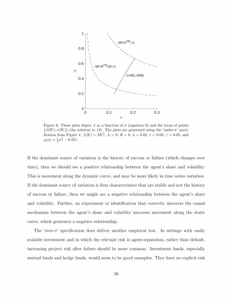
have opposite signs. We illustrate this in Figure 6, where the solid line is how the economy

evolves as a function of W , and the dashed lines are the function β(K, σ) for two different

values of K.

Empirically, this result means that our model predicts different results for time series and

cross-sectional tests in the ‘under-σ’ specification, because the source of variation is different.

37

0 0.1 0.2 0.3<

0

0.2

0.4

0.6

0.8

1

-

-(K=KFB,<)

-(K=KFB/10,<)

<(W),-(W)

Figure 6: These plots depict β as a function of σ (equation 9) and the locus of pointsβ(W ), σ(W ) (the solution to 12). The plots are generated using the ‘under-σ’ speci-

fication from Figure 4: f(K) = 2K12 , L = 0, R = 0, λ = 0.02, r = 0.03, γ = 0.05, and

µ(σ) = 13σ

12 − 0.37σ.

If the dominant source of variation is the history of success or failure (which changes over

time), then we should see a positive relationship between the agent’s share and volatility.

This is movement along the dynamic curve, and may be more likely in time series variation.

If the dominant source of variation is firm characteristics that are stable and not the history

of success or failure, then we might see a negative relationship between the agent’s share

and volatility. Further, an experiment or identification that correctly uncovers the causal

mechanism between the agent’s share and volatility uncovers movement along the static

curve, which generates a negative relationship.

The ‘over-σ’ specification does deliver another empirical test. In settings with easily

scalable investment and in which the relevant risk is agent-separation, rather than default,

increasing project risk after failure should be more common. Investment funds, especially

mutual funds and hedge funds, would seem to be good examples. They have no explicit risk

38

of default, and to the extent that fund manager skill is real, the primary danger to fund

value is that the high-skill manager leaves. In fact, many empirical results, (e.g. Chevalier

and Ellison (1997), Aragon and Nanda (2011), Huang et al. (2011)) find increasing project

risk after failure to be the case. However, those studies often attribute the increase in risk

to convex incentive schemes. Our mechanism is different: increasing project risk actually

decreases termination risk. A useful empirical test would be to distinguish changes in inside

and outside values, and to see to what extent that difference impacts investment risk.

6 Further Discussion

It is useful to connect two aspects of our model to analogous models of hidden effort, such

as DeMarzo and Sannikov (2006) and Zhu (2013). In particular, Zhu (2013) shows that the

principal can relax incentives to either pay the agent with private benefits instead of cash or

relax incentives to prevent termination/default after bad cash-flow realizations. Our model

does have an incentives shutdown (Property 6), but the mechanism is different from that in

Zhu (2013).

We first consider the left boundary–preventing termination by reducing incentives. In

our model, the principal has to pay an ongoing rental cost of capital (rKt) in order to

fund the project; the amount of capital determines the project’s scale and the potential

private benefits available to the agent. Since paying the agent with private benefits delivers

benefits that are less than the rental cost of capital (λ ≤ r), the principal will always couple

zero incentives with zero project size. This prevents the agent from receiving additional

negative cash0flow shocks, so the agent’s continuation value drifts upward, and the project

can continue.

In contrast, Zhu (2013) has fixed project scale, and so when incentives are relaxed the

principal cannot also restrict private benefits to the agent. This makes the principal worse

39

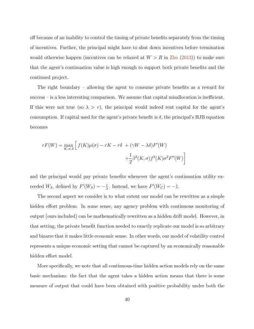
off because of an inability to control the timing of private benefits separately from the timing

of incentives. Further, the principal might have to shut down incentives before termination

would otherwise happen (incentives can be relaxed at W > R in Zhu (2013)) to make sure

that the agent’s continuation value is high enough to support both private benefits and the

continued project.

The right boundary – allowing the agent to consume private benefits as a reward for

success – is a less interesting comparison. We assume that capital misallocation is inefficient.

If this were not true (so λ > r), the principal would indeed rent capital for the agent’s

consumption. If capital used for the agent’s private benefit is δ, the principal’s HJB equation

becomes

rF (W ) = maxK,σ, δ

[f(K)µ(σ)− rK − rδ + (γW − λδ)F ′(W )

+1

2β2(K, σ)f 2(K)σ2F ′′(W )

]

and the principal would pay private benefits whenever the agent’s continuation utility ex-

ceeded WS, defined by F ′(WS) = − rλ. Instead, we have F ′(WC) = −1.

The second aspect we consider is to what extent our model can be rewritten as a simple

hidden effort problem. In some sense, any agency problem with continuous monitoring of

output (ours included) can be mathematically rewritten as a hidden drift model. However, in

that setting, the private benefit function needed to exactly replicate our model is so arbitrary

and bizarre that it makes little economic sense. In other words, our model of volatility control

represents a unique economic setting that cannot be captured by an economically reasonable

hidden effort model.

More specifically, we note that all continuous-time hidden action models rely on the same

basic mechanism: the fact that the agent takes a hidden action means that there is some

measure of output that could have been obtained with positive probability under both the

40

agent’s true action and under the principal’s desired action. If the cash flow contains a

Brownian motion, that means the entire space of hidden action models is contained in one

meta-model in which the agent controls the drift of the Brownian motion. Our model is no

different: we can write dYt = f(Kt)etdt + ΣtdZt instead of (1), using et = f(Kt)f(Kt)

µ(

Σt

f(Kt)

)as the hidden action instead of Kt. Then, the agent’s private benefits function becomes

B(e,K,Σ) = λ(K − K(e,K,Σ)

), where K(et, Kt,Σt) is an inversion of e(K,K,Σ). All our

results would follow under a change of variables.

However, this change of variables puts all the economics into the private benefits function

in a completely uninterpretable way. First, B(e,K,Σ) has unsigned derivatives (i.e. BK and

BΣ change signs over the relevant range of the problem). Second, even the level of private

benefits is difficult to assess because the constraint B(e(K,K,Σ), K,Σ) = 0 is a technological

constraint that must be imposed exogenously. Instead, we put structure on the production

function (f(K)µ(σ)), which makes it clear that the shape of our problem is economically

motivated. Third, the proposed change of variables makes it impossible to talk about risk or

volatility as an agency problem. The first contribution of our model is to show that agency

problems over the composition of volatility are possible and interesting – total cash-flow

volatility (Σ), project volatility (σ), and agent’s continuation value volatility (βσ) are all

meaningfully different.

7 Conclusion

Since DeMarzo and Sannikov (2006), Biais et al. (2007), and Sannikov (2008), continuous-

time principal-agent models have developed rapidly with applications to expanding areas of

economic research. Despite the progress, almost all of the existing models involve the agent

controlling the drift of the output/cash-flow process. We deviate from the literature by

considering the optimal contract when the agent controls the volatility. Our major technical

41

obstacle is that volatility of Brownian motion is observable. To establish a meaningful

volatility control model, we consider the case where overall cash flow is made up of two

components: the individual risk of the project and capital intensity, both of which are

observable only to the agent. The principal must incentivize the agent to choose the desirable

level of project risk and capital intensity. Interestingly, such incentives can be implemented

without loss of generality with a simple hurdle rate against which the agent’s performance–

the realized cash flow – is measured. The agent is allowed to propose the level of risk and

the amount of capital he wants, even his compensation – his share of the cash-flow residual,

and the hurdle rate takes the form of a time-varying cost of capital adjusted for the risk and

capital intensity of the agent’s proposal.

The ideas in our model can be broadened in several ways. One is to extend the literature

on optimal disclosure to endogenize the frequency of observation. Another interesting direc-

tion is to find asset pricing implications (e.g. Buffa et al. (2015)) of the optimal contract.

As our model applies to an asset manager who can privately choose his portfolio, how the

manager’s contract and the equilibrium asset price are jointly determined would be a natural

question to explore.

42

Appendix

Proof of Proposition 1

First17, we define the agent’s total expected utility received under a contract conditional onhis information at time t as:

Ut = EK, σ

[∫ τ

0

e−γudCu +

∫ τ

0

e−γuλ∆udu+ e−γτR |Ft],

where ∆u = Ku−Ku. We note that the process U = Ut,Ft; 0 ≤ t < τ is an Ft-martingale.The expectation is taken with respect to the probability measure induced by K, σ, such

that dZK, σt = 1

Σt

(dYt − f(Kt)µ(σt)dt

)is a Brownian motion. Then, by the martingale

representation theorem for Levy processes, there exists a Ft-predictable process β such that

Ut = U0 +

∫ t

0

e−γuβuΣudZK, σu . (24)

Recall the agent’s continuation value W K, σt defined in (4), we have

Ut =

∫ t

0

e−γudCu +

∫ t

0

e−γuλ∆udu+ e−γtW K, σt . (25)

for t ≤ τ . Differentiating (24) and (25), we obtain

dUt = e−γtβtΣtdZK, σt = e−γtdCt + e−γtλ∆tdt− γe−γtW K, σ

t dt+ e−γtdW K, σt ,

therefore

dW K, σt = γW K, σ

t dt− dCt − λ∆tdt+ βtΣtdZK, σt .

This equation also implies the evolution of promised value given in (8) for K, σ = K, σ.Next, define Ut to be the payoff to a strategy K, σ that consists of following an arbitrary

strategy until time t < τ and then K, σ thereafter, then

Ut =

∫ t

0

e−γudCu +

∫ t

0

e−γuλ∆udu+ e−γtWK,σt .

17This proof a slightly modified version of a proof in Piskorski and Westerfield (2016), which in turn isbased on a similar proof in Sannikov (2008).

43

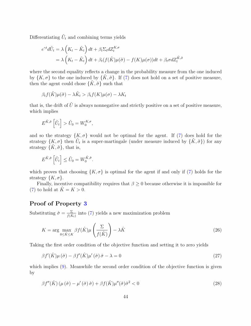
Differentiating Ut and combining terms yields

eγtdUt = λ(Kt − Kt

)dt+ βtΣtdZ

K,σt

= λ(Kt − Kt

)dt+ βt(f(K)µ(σ)− f(K)µ(σ))dt+ βtσdZ

K,σt

where the second equality reflects a change in the probability measure from the one inducedby K, σ to the one induced by K, σ. If (7) does not hold on a set of positive measure,then the agent could chose K, σ such that

βtf(K)µ(σ)− λKt > βtf(K)µ(σ)− λKt

that is, the drift of U is always nonnegative and strictly positive on a set of positive measure,which implies

EK,σ[Ut

]> U0 = WK,σ

0 ,

and so the strategy K, σ would not be optimal for the agent. If (7) does hold for thestrategy K, σ then Ut is a super-martingale (under measure induced by K, σ) for anystrategy K, σ, that is,

EK,σ[Ut

]≤ U0 = W K,σ

0 .

which proves that choosing K, σ is optimal for the agent if and only if (7) holds for thestrategy K, σ.

Finally, incentive compatibility requires that β ≥ 0 because otherwise it is impossible for(7) to hold at K = K > 0.

Proof of Property 3

Substituting σ = Σ

f(Kt)into (7) yields a new maximization problem

K = arg max0≤K≤K

βf(K)µ

(Σ

f(K)

)− λK (26)

Taking the first order condition of the objective function and setting it to zero yields

βf ′(K)µ (σ)− βf ′(K)µ′ (σ) σ − λ = 0 (27)

which implies (9). Meanwhile the second order condition of the objective function is givenby

βf ′′(K) (µ (σ)− µ′ (σ) σ) + βf(K)µ′′(σ)σ2 < 0 (28)

44

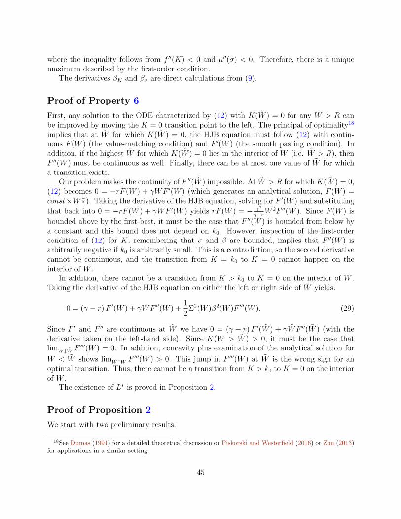
where the inequality follows from f ′′(K) < 0 and µ′′(σ) < 0. Therefore, there is a uniquemaximum described by the first-order condition.

The derivatives βK and βσ are direct calculations from (9).

Proof of Property 6

First, any solution to the ODE characterized by (12) with K(W ) = 0 for any W > R canbe improved by moving the K = 0 transition point to the left. The principal of optimality18

implies that at W for which K(W ) = 0, the HJB equation must follow (12) with contin-uous F (W ) (the value-matching condition) and F ′(W ) (the smooth pasting condition). Inaddition, if the highest W for which K(W ) = 0 lies in the interior of W (i.e. W > R), thenF ′′(W ) must be continuous as well. Finally, there can be at most one value of W for whicha transition exists.

Our problem makes the continuity of F ′′(W ) impossible. At W > R for which K(W ) = 0,(12) becomes 0 = −rF (W ) + γWF ′(W ) (which generates an analytical solution, F (W ) =const×W

rg ). Taking the derivative of the HJB equation, solving for F ′(W ) and substituting

that back into 0 = −rF (W ) + γWF ′(W ) yields rF (W ) = − γ2

γ−rW2F ′′(W ). Since F (W ) is

bounded above by the first-best, it must be the case that F ′′(W ) is bounded from below bya constant and this bound does not depend on k0. However, inspection of the first-ordercondition of (12) for K, remembering that σ and β are bounded, implies that F ′′(W ) isarbitrarily negative if k0 is arbitrarily small. This is a contradiction, so the second derivativecannot be continuous, and the transition from K = k0 to K = 0 cannot happen on theinterior of W .

In addition, there cannot be a transition from K > k0 to K = 0 on the interior of W .Taking the derivative of the HJB equation on either the left or right side of W yields:

0 = (γ − r)F ′(W ) + γWF ′′(W ) +1

2Σ2(W )β2(W )F ′′′(W ). (29)

Since F ′ and F ′′ are continuous at W we have 0 = (γ − r)F ′(W ) + γWF ′′(W ) (with thederivative taken on the left-hand side). Since K(W > W ) > 0, it must be the case thatlimW↓W F ′′′(W ) = 0. In addition, concavity plus examination of the analytical solution for

W < W shows limW↑W F ′′′(W ) > 0. This jump in F ′′′(W ) at W is the wrong sign for anoptimal transition. Thus, there cannot be a transition from K > k0 to K = 0 on the interiorof W .

The existence of L∗ is proved in Proposition 2.

Proof of Proposition 2

We start with two preliminary results:

18See Dumas (1991) for a detailed theoretical discussion or Piskorski and Westerfield (2016) or Zhu (2013)for applications in a similar setting.

45

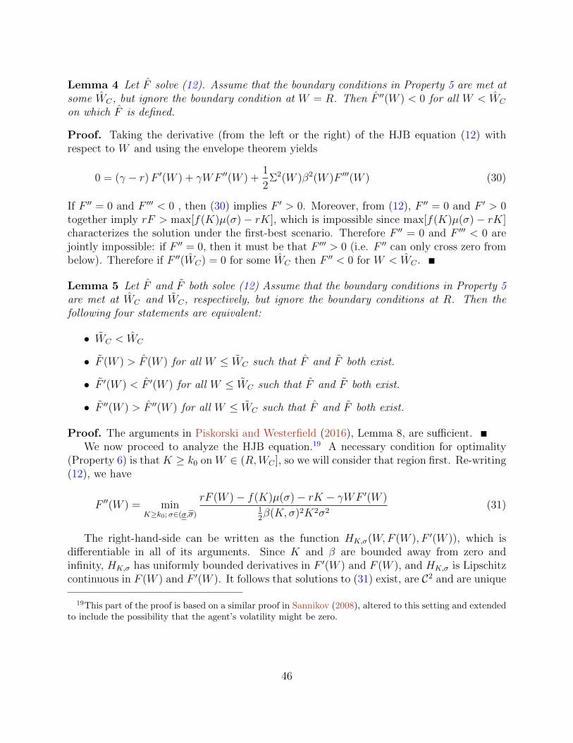
Lemma 4 Let F solve (12). Assume that the boundary conditions in Property 5 are met atsome WC, but ignore the boundary condition at W = R. Then F ′′(W ) < 0 for all W < WC

on which F is defined.

Proof. Taking the derivative (from the left or the right) of the HJB equation (12) withrespect to W and using the envelope theorem yields

0 = (γ − r)F ′(W ) + γWF ′′(W ) +1

2Σ2(W )β2(W )F ′′′(W ) (30)

If F ′′ = 0 and F ′′′ < 0 , then (30) implies F ′ > 0. Moreover, from (12), F ′′ = 0 and F ′ > 0together imply rF > max[f(K)µ(σ)− rK], which is impossible since max[f(K)µ(σ)− rK]characterizes the solution under the first-best scenario. Therefore F ′′ = 0 and F ′′′ < 0 arejointly impossible: if F ′′ = 0, then it must be that F ′′′ > 0 (i.e. F ′′ can only cross zero frombelow). Therefore if F ′′(WC) = 0 for some WC then F ′′ < 0 for W < WC .

Lemma 5 Let F and F both solve (12) Assume that the boundary conditions in Property 5are met at WC and WC, respectively, but ignore the boundary conditions at R. Then thefollowing four statements are equivalent:

• WC < WC

• F (W ) > F (W ) for all W ≤ WC such that F and F both exist.

• F ′(W ) < F ′(W ) for all W ≤ WC such that F and F both exist.

• F ′′(W ) > F ′′(W ) for all W ≤ WC such that F and F both exist.

Proof. The arguments in Piskorski and Westerfield (2016), Lemma 8, are sufficient.We now proceed to analyze the HJB equation.19 A necessary condition for optimality

(Property 6) is that K ≥ k0 on W ∈ (R,WC ], so we will consider that region first. Re-writing(12), we have

F ′′(W ) = minK≥k0;σ∈(σ,σ)

rF (W )− f(K)µ(σ)− rK − γWF ′(W )12β(K, σ)2K2σ2

(31)

The right-hand-side can be written as the function HK,σ(W,F (W ), F ′(W )), which isdifferentiable in all of its arguments. Since K and β are bounded away from zero andinfinity, HK,σ has uniformly bounded derivatives in F ′(W ) and F (W ), and HK,σ is Lipschitzcontinuous in F (W ) and F ′(W ). It follows that solutions to (31) exist, are C2 and are unique

19This part of the proof is based on a similar proof in Sannikov (2008), altered to this setting and extendedto include the possibility that the agent’s volatility might be zero.

46

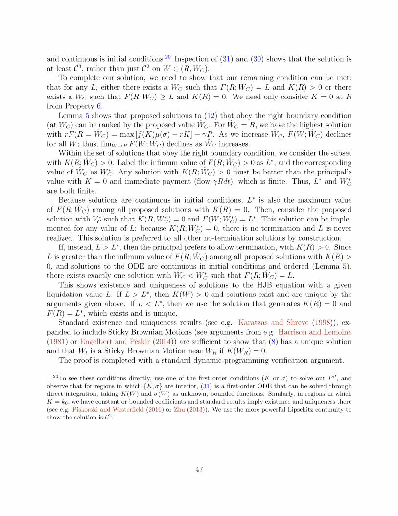
and continuous is initial conditions.20 Inspection of (31) and (30) shows that the solution isat least C3, rather than just C2 on W ∈ (R,WC).

To complete our solution, we need to show that our remaining condition can be met:that for any L, either there exists a WC such that F (R;WC) = L and K(R) > 0 or thereexists a WC such that F (R;WC) ≥ L and K(R) = 0. We need only consider K = 0 at Rfrom Property 6.

Lemma 5 shows that proposed solutions to (12) that obey the right boundary condition(at WC) can be ranked by the proposed value WC . For WC = R, we have the highest solutionwith rF (R = WC) = max [f(K)µ(σ)− rK] − γR. As we increase WC , F (W ; WC) declinesfor all W ; thus, limW→R F (W ; WC) declines as WC increases.

Within the set of solutions that obey the right boundary condition, we consider the subsetwith K(R; WC) > 0. Label the infimum value of F (R; WC) > 0 as L∗, and the correspondingvalue of WC as W ∗

C . Any solution with K(R; WC) > 0 must be better than the principal’svalue with K = 0 and immediate payment (flow γRdt), which is finite. Thus, L∗ and W ∗

C

are both finite.Because solutions are continuous in initial conditions, L∗ is also the maximum value

of F (R; WC) among all proposed solutions with K(R) = 0. Then, consider the proposedsolution with V ∗C such that K(R,W ∗

C) = 0 and F (W ;W ∗C) = L∗. This solution can be imple-

mented for any value of L: because K(R;W ∗C) = 0, there is no termination and L is never

realized. This solution is preferred to all other no-termination solutions by construction.If, instead, L > L∗, then the principal prefers to allow termination, with K(R) > 0. Since

L is greater than the infimum value of F (R; WC) among all proposed solutions with K(R) >0, and solutions to the ODE are continuous in initial conditions and ordered (Lemma 5),there exists exactly one solution with WC < W ∗

C such that F (R; WC) = L.This shows existence and uniqueness of solutions to the HJB equation with a given

liquidation value L: If L > L∗, then K(W ) > 0 and solutions exist and are unique by thearguments given above. If L < L∗, then we use the solution that generates K(R) = 0 andF (R) = L∗, which exists and is unique.

Standard existence and uniqueness results (see e.g. Karatzas and Shreve (1998)), ex-panded to include Sticky Brownian Motions (see arguments from e.g. Harrison and Lemoine(1981) or Engelbert and Peskir (2014)) are sufficient to show that (8) has a unique solutionand that Wt is a Sticky Brownian Motion near WR if K(WR) = 0.

The proof is completed with a standard dynamic-programming verification argument.

20To see these conditions directly, use one of the first order conditions (K or σ) to solve out F ′′, andobserve that for regions in which K,σ are interior, (31) is a first-order ODE that can be solved throughdirect integration, taking K(W ) and σ(W ) as unknown, bounded functions. Similarly, in regions in whichK = k0, we have constant or bounded coefficients and standard results imply existence and uniqueness there(see e.g. Piskorski and Westerfield (2016) or Zhu (2013)). We use the more powerful Lipschitz continuity toshow the solution is C2.

47

Proof of Property 8

The principal’s HJB equations (16 and 17) and the accompanying first-order conditions are

rF (W ) = maxK,σ

[CF (K, σ) + γWF ′(W ) +

1

2g(K)2h(σ)2F ′′(W )

]FOC(K) : CFK(K, σ) + g′(K)g(K)h2(σ)F ′′(W )

FOC(σ) : CFσ(K, σ) + g2(K)h′(σ)h(σ)F ′′(W )

and

rF (W ) = maxΣ, β

[CF (Σ, β) + γWF ′(W ) +

1

2Σ2β2F ′′(W )

]FOC(Σ) : CFΣ(Σ, β) + Σβ2F ′′(W )

FOC(β) : CFβ(Σ, β) + Σ2βF ′′(W )

where CF (K, σ) = f(K)µ(σ) − rK, g(K) = f(K)/f ′(K), h(σ) = λσ/(µ(σ) − σµ′(σ)).Assumption 1 is sufficient to ensure strict concavity of the HJB equation with respect to Kand σ. Signing g′(K) and h′(σ), remembering that F ′′(W ) ≤ 0, and evaluating the first-orderconditions directly, are sufficient to demonstrate the statement of the property with respectto K and σ.

Next, we rewrite the cash flow as CF (β,Σ) = CF (K(β,Σ), σ(β,Σ)). Because thefirst-best has CFK(KFB, σFB) = CFσ(KFB, σFB) = 0, there is a corresponding value of(βFB,ΣFB) which has CFK(K(βFB,ΣFB), σ(βFB,ΣFB)) = CFσ(K(βFB,ΣFB), σ(βFB,ΣFB)) =0. The second order conditions for the HJB equation (17), evaluated at βFB,ΣFB are

SOC(β)|(βFB ,ΣFB) : CFKK · (Kβ)2 + CFσσ · (σβ)2 < 0 (32)

SOC(Σ)|(βFB ,ΣFB) : CFKK · (KΣ)2 + CFσσ · (σΣ)2 < 0, (33)

where the inequalities follow from CFKK < 0 and CFσσ < 0. Because the first-best is unique,with CFβ = 0 and CFΣ = 0, we also have that CFβ > 0 implies β < βFB and CFΣ > 0implies Σ < ΣFB. Combining this with the first-order conditions (17) yields the statementof the property.

Proof of Property 10

Assume that the principal offers the agent a recommended level of capital misallocation, δt,to go with the assigned level of capital, Kt + δt. Then the contract is incentive compatibleif it implements Kt = Kt and δt = δt. The incentive compatibility condition (7) becomes

Kt, δt, σt = arg maxKt+δt=Kt+δt; f(Kt)σt=f(Kt)σt

[βtf(Kt)µ(σt) + λ

(Kt + δt − Kt

)]. (34)

48

Note that the agent-controlled portion of the right-hand side is the same as in the originalIC condition (7). The first order conditions imply that βt becomes

βt = β(σt, Kt) =λ

f ′(Kt)× 1

µ(σt)− µ′(σt)σt. (35)

The evolution of the agent’s continuation value becomes

dWt = γWtdt+ βtΣtdZt − λδtdt− dCt . (36)

The principal’s HJB equation (12) becomes

rF (W ) = maxK+δ∈0∪[k0,∞);σ∈(σ,σ)

[f(K)µ(σ)− rK − rδ + (γW − λδ)F ′(W )

+1

2β2(K, σ)f 2(K)σ2F ′′(W )

](37)

For any given choice of K, the objective function of (37) is linear in δ with coefficient−r − λF ′(W ). Since F ′(W ) ≥ −1, we have −r − λF ′(W ) < 0. Therefore, δ = 0 is (weakly)optimal.

Proof of Proposition 3

The principal offers the agent the adjusted technology with

dYt = f(Kt)µ

(Σt

f(Kt)

)dt− Ktθ(βt, Σt)dt+ ΣtdZt.

Then we define the probability measure induced by K, Σ, β, K to be such that

dZK,Σ,β,Kt =

1

Σt

(dYt − f(K)µ

(Σ

f(K)

)dt+ Ktθ(βt, Σt)dt

)

is a Brownian motion. We do not need to include σ because Σ and K determine σ.The arguments in the proof of Proposition 1 follow, with the modification that the agent’s

incentive compatibility condition is (22) instead of (7), The condition on φ in (22) is setso that the drift in the agent’s continuation utility, given by (21), equals γWt. That is,

dWt = γWtdt + βtΣtdZK,Σ,β,Kt − dCt. If the agent’s maximizing choices are K, Σ, β, K =

K,Σ, β,K then the principal’s problem is unchanged, there is no capital misallocation, andcash flow is unchanged. To implement K = 0, the principal simply offers φt, θt = 0,∞,or mandates shutdown.

49

Substituting θ(β, Σ) = λ/β + [b(β − β)]+ + [c(Σ− Σ)]+ into (22) yields

φ = maxK≥k0; Σ>0; β>0; K≥K≥0

[βf(K)µ

(Σ

f(K)

)− λK

−βK(

[b(β − β)]+ + [c(Σ− Σ)]+)]

(38)

We first examine the case where b(β − β) ≥ 0 and c(Σ− Σ) ≥ 0. Observe that Assump-tion 1 implies that the second order conditions for K, Σ, and β are strictly negative. Thesecond-order condition for K is equal to zero and the first-order condition is less than orequal to zero; we assume the agent picks the principal’s desired level of K if he is indifferent.As a result, the agent’s optimal choices are given by the first-order conditions:

FOC(K) : − β(b(β − β) + c(Σ− Σ)+

)FOC(Σ) : β

[µ′

(Σ

f(K)

)− cK

]

FOC(β) : f(K)µ

(Σ

f(K)

)− K

(b(2β − β) + c(Σ− Σ)

)FOC(K) : β

[f ′(K)µ

(Σ

f(K)

)− µ′

(Σ

f(K)

)Σ

f(K)

]− λ

Recall that the value of β in the optimal contract exactly induces no capital misalloca-tion (K = K). Standard algebra shows that the above first-order conditions are zero atK, Σ, β, K = K,Σ, β,K if the principal chooses

Kβb = f(K)µ

(Σ

f(K)

)c =

1

Kµ′(

Σ

f(K)

)In addition, evaluating (38) at the optimum implies

φ = βf(K)µ

(Σ

f(K)

)−Kλ.

We now verify that given a, b, c above, any choice of β and Σ such that either b(β−β) < 0or c(Σ−Σ) < 0 cannot be the agent’s solution to (38). First, b > 0, which implies b(β−β) < 0if and only if β < β. However, this cannot be optimal, as the agent can increase β whileholding his other choices constant. This would increase the first term on the right-hand-side

of (38) while other terms remain unchanged. Secondly, c > 0 if µ′(

Σf(K)

)> 0, which implies

50

c(Σ − Σ) < 0 if and only if Σ < Σ. However, this cannot be optimal, as the agent canincrease Σ while holding his other choices constant. This would increase the first term onthe right-hand-side of (38) while other terms remain unchanged. The same argument applies

if c < 0 because µ′(

Σf(K)

)< 0, which implies it is not optimal for the agent to choose Σ > Σ.

Therefore, setting θ(β, Σ) = λβ

+[b(β−β)]+ +[c(Σ−Σ)]+ where a, b, c are given above ensures

(38) achieves it maximum when K = K = K; Σ = Σ; β = β.

51

References

Adrian, T. and M. M. Westerfield (2009). Disagreement and learning in a dynamic contract-ing model. Review of Financial Studies 22 (10), 3829–3871.

Aragon, G. O. and V. Nanda (2011). Tournament behavior in hedge funds: High-watermarks, fund liquidation, and managerial stake. Review of Financial Studies 25 (3), 937–974.

Bertrand, M. and S. Mullainathan (2003). Enjoying the quiet life? Corporate governanceand managerial preferences. Journal of Political Economy 111 (5), 1043–1075.

Biais, B., T. Mariotti, G. Plantin, and J.-C. Rochet (2007). Dynamic security design: Con-vergence to continuous time and asset pricing implications. Review of Economic Studies 74,345–390.

Biais, B., T. Mariotti, J.-C. Rochet, and S. Villeneuve (2010). Large risks, limited liability,and dynamic moral hazard. Econometrica 78, 73–118.

Buffa, A. M., D. Vayanos, and P. Woolley (2015). Asset management contracts and equilib-rium prices. NBER working paper.

Cadenillas, A., J. Cvitanic, and F. Zapatero (2004). Leverage decision and manager com-pensation with choice of effort and volatility. Journal of Financial Economics 73 (1),71–92.

Carpenter, J. N. (2000). Does option compensation increase managerial risk appetite? Jour-nal of Finance 55 (5), 2311–2331.

Chevalier, J. and G. Ellison (1997). Risk taking by mutual funds as a response to incentives.The Journal of Political Economy 105 (6), 1167–1200.

Cremers, M. and A. Petajisto (2009). How active is your fund manager? A new measurethat predicts performance. Review of Financial Studies 22 (9), 3329–3365.

Cvitanic, J., D. Possamaı, and N. Touzi (2016a). Dynamic programming approach toprincipal-agent problems. Working Paper, Caltech, University Paris-Dauphine, and EcolePolytechnique.

Cvitanic, J., D. Possamaı, and N. Touzi (2016b). Moral hazard in dynamic risk management.Management Science. forthcoming.

DeMarzo, P. and Y. Sannikov (2006). Optimal security design and dynamic capital structurein a continuous-time agency model. Journal of Finance 61, 2681–2724.

DeMarzo, P. M., M. J. Fishman, Z. He, and N. Wang (2012). Dynamic agency and the qtheory of investment. Journal of Finance 67 (6), 2295–2340.

52

Dumas, B. (1991). Super contact and related optimality conditions. Journal of EconomicDynamics and Control 75 (4), 675–685.

Engelbert, H.-J. and G. Peskir (2014). Stochastic differential equations for sticky brownianmotion. Stochastics 86 (6), 993–1021.

Epstein, L. G. and S. Ji (2013). Ambiguous volatility and asset pricing in continuous time.Review of Financial Studies 26 (7), 1740–1786.

Giroud, X. (2013). Proximity and investment: Evidence from plant-level data. QuarterlyJournal of Economics 128 (2), 861–915.

Graham, J. and C. Harvey (2011). Duke/CFO magazine global business outlook. U.S.topline tables, March 2011, www.cfosurvey.org/pastresults.htm.

Graham, J. and C. Harvey (2012). Duke/CFO magazine global business outlook. U.S.topline tables, June 2012, www.cfosurvey.org/pastresults.htm.

Graham, J. R. and C. R. Harvey (2001). The theory and practice of corporate finance:Evidence from the field. Journal of Financial Economics 60 (2), 187–243.

Harrison, J. M. and A. J. Lemoine (1981). Sticky brownian motion as the limit of storageprocesses. Journal of Applied Probability 18 (1), 216–226.

He, Z. (2011). A model of dynamic compensation and capital structure. Journal of FinancialEconomics 100 (2), 351–366.

Huang, J., C. Sialm, and H. Zhang (2011). Risk shifting and mutual fund performance.Review of Financial Studies 24 (8), 2575–2616.

Jacobs, M. T. and A. Sivdasani (2012). Do you know your cost of capital? Harvard BusinessReview (7/8), 118–124.

Jagannathan, R., D. A. Matsa, I. Meier, and V. Tarhan (2016). Why do firms use highdiscount rates? Journal of Financial Economics , 445–463.

Karatzas, I. and S. Shreve (1998). Brownian Motion and Stochastic Calculus (2nd ed.).Springer-Verlag New York.

Leung, R. (2014). Continuous-time principal-agent problem with drift and stochastic volatil-ity control: With applications to delegated portfolio management. Working paper. Uni-versity of California-Berkeley.

Lioui, A. and P. Poncet (2013). Optimal benchmarking for active portfolio managers. Eu-ropean Journal of Operational Research 226 (2), 268–276.

Metrick, A. and A. Yasuda (2010). The economics of private equity funds. Review ofFinancial Studies 23 (6), 2303–2341.

53

Moreno-Bromberg, S. and G. Roger (2016). Leverage and risk taking. Working Paper,University of Zurich and University of Sydney.

Ou-Yang, H. (2003). Optimal contracts in a continuous-time delegated portfolio managementproblem. Review of Financial Studies 16 (1), 173–208.

Piskorski, T. and M. M. Westerfield (2016). Optimal dynamic contracts with moral hazardand costly monitoring. Journal of Economic Theory 166, 242–281.

Poterba, J. M. and L. H. Summers (1995). A CEO survey of U.S. companies’ time horizonsand hurdle rates. MIT Sloan Management Review (Fall), 43–53.

Prendergast, C. (2002). The tenuous trade-off between risk and incentives. Journal ofPolitical Economy 110 (5), 1071–1102.

Robinson, D. T. and B. A. Sensoy (2013). Do private equity fund managers earn their fees?Compensation, ownership, and cash flow performance. Review of Financial Studies 26 (11),2760–2797.

Sannikov, Y. (2008). A continuous-time version of the principal-agent problem. Review ofEconomic Studies 75, 957–984.

Zhu, J. Y. (2013). Optimal contracts with shirking. Review of Economic Studies 80, 812–839.

54