Information Processing Letters 110 (2010) 1049–1054

Contents lists available at ScienceDirect

Information Processing Letters

www.elsevier.com/locate/ipl

Dynamic bin packing with unit fraction items revisited

Xin Han a,∗,1, Chao Peng b, Deshi Ye c,2, Dahai Zhang d, Yan Lan e

a School of Software of Dalian University of Technology, Chinab Shanghai Key Laboratory of Trustworthy Computing, School of Software Engineering, East China Normal University, Shanghai 200062, Chinac College of Computer Science, Zhejiang University, Hangzhou 310027, Chinad Key Laboratory of Marine Chemistry Theory and Technology, Ministry of Education, Ocean University of China, Qingdao 266100, Chinae Dalian Neusoft Institute of Information, China

a r t i c l e i n f o a b s t r a c t

Article history:Received 14 January 2010Received in revised form 23 August 2010Accepted 1 September 2010Available online 20 September 2010Communicated by F.Y.L. Chin

Keywords:Approximation algorithmsCompetitive ratioBin packing problem

In this paper, we will study the problem of dynamic bin packing with unit fraction items.We focus on analyzing the First Fit (FF) algorithm on this problem. There are two mainresults: i) we give the first bound for the FF algorithm on cases when the largest item is atmost 1/k; ii) we generalize the previous framework for analyzing FF and get an improvedupper bound.

© 2010 Elsevier B.V. All rights reserved.

1. Introduction

Bin packing problem is a classical problem in computerscience and operations research [11,12,5,14,15]. In this pa-per, we study the dynamic bin packing problem [9], whichis formulated as below:

Dynamic bin packingInput: An infinite number of unit size bins B and a finite

sequence or list L = (p1, p2, . . . , pn), where an item orpiece pi in L corresponds to a triple (ai,di, si) and ai

is the arrival time, di is the departure time, while si

is the size. The item pi resides in the packing for thetime interval [ai,di), where di − ai > 0 for all i. Weassume that 0 < si � 1 for all i, and a1 � a2 � · · · � an .

* Corresponding author.E-mail addresses: hanxin.mail@gmail.com (X. Han),

cpeng@sei.ecnu.edu.cn (C. Peng), yedeshi@zju.edu.cn (D. Ye),haidadedahai@hotmail.com (D. Zhang), lanyan@neusoft.edu.cn (Y. Lan).

1 Partially supported by “the Fundamental Research Funds for the Cen-tral Universities”.

2 Partially supported by the funding NSFC (11071215).

0020-0190/$ – see front matter © 2010 Elsevier B.V. All rights reserved.doi:10.1016/j.ipl.2010.09.002

Output: Pack all the items in L into the set of bins B tominimize the maximum number of bins ever used inprocessing L.

Dynamic bin packing with unit fraction items: We studydynamic bin packing of unit fraction items. A unit frac-tion item has size of the form 1/i for some integer i.

There are two versions, online and offline dynamic binpacking problems. In the offline dynamic bin packing, thewhole information about L, i.e., all the values of ai,di, si ,are known before packing. In the online setting, items ar-rive over time, i.e., after we handle all the items given sofar, the information of the next item is known. Note that di

is not known at the arrival ai , but only known at the timewhen item pi leaves. And repacking is not allowed, i.e.,once an item is assigned into a bin, it cannot be movedinto another bin in the future. As mentioned in the pa-per [9], the online model is motivated by applications suchas dynamic storage allocation. The online model arises alsoin virtual computing environment. Recently, virtual ma-chines and multi-core bring much challenge in operatingsystems. In such a computing system [2], a virtual machinemonitor dynamically opens or destroys virtual machinesaccording to the users’ requirement, and maps each vir-

1050 X. Han et al. / Information Processing Letters 110 (2010) 1049–1054

Table 1In bin packing problems, the largest item is at most 1/k, the results in the second row are the upper bounds of FF for the general dynamic bin packing(DBP), the results in the last row are the upper bounds of FF for DBP with unit fraction items.

k 2 3 4 5 6 7 8 9 10

Old [9] 1.7877 1.4590 1.3192 1.2436 1.1966 1.1646 1.1415 1.1241 1.1105New 1.7111 1.4354 1.3094 1.2387 1.1938 1.1629 1.1404 1.1233 1.1099

tual machine to one core. The required CPU time of eachvirtual machine can be regarded as the load in the corre-sponding core. Hence, our problem represents the dynamicload balancing problem among the cores.

Given an online algorithm A and an input sequence L,let A(L, t) denote the number of occupied bins in packingL by A at time t . We use the following definition to mea-sure the performance of algorithm A with respect to theinput L,

A(L) = max0�t�an

A(L, t),

i.e., A(L) is the maximum number of occupied bins everused by algorithm A in packing L.

Let OPT(L) be the maximum number of bins ever usedin packing L where repacking is allowed any time. Definethe asymptotic competitive ratio of an online algorithm Awith respect to OPT(L) as follows:

R(A) = limm→∞ sup max

L

{A(L)/OPT(L) | OPT(L) = m

}.

If R(A) = α then it means that for any input L we have

A(L) � α · OPT(L) + O (1).

Previous results. For the problem with general size items,Coffman et al. gave the first upper bound 2.788 based onthe online algorithm FF [9]. They also proved that if thelargest item has size at most 1

k , where k � 2, then the FF

algorithm has competitive ratio k+1k + 1

k−1 ln( k2

k2−k+1) [9].

No online algorithm can achieve a competitive ratio bet-ter than 2.5 [9], even the offline optimal algorithm is notallowed to repack items [8]. Ivkovic et al. [13] gave a 1.25-competitive online algorithm for the problem if repackingitems are allowed where the total space for repacking ineach step is bounded by a constant. If each step the num-ber of repacking items is limited to a constant, Balogh et al.[1] showed that no online algorithm can get a competi-tive ratio better than 1.3871. And resource augmentationanalysis for the problem was studied in [8]. For the prob-lem with unit fraction items, Chan et al. showed that FFhas a competitive ratio at most 2.4942 and FF has a com-petitive ratio at least 2.45, and they also proved that noonline algorithm has a competitive ratio better than 2.428[6]. The problem with unit fraction items is also relatedto the windows scheduling problem [3,4,7] and bin packingwith divisible item sizes [10].

Our contribution. There are two main contributions onthe problem with unit fraction items. i) We obtain the firstbound for the parameter case which is better than thegeneral case in [9] (see Table 1), where the largest item

is bounded by 1/k, and our approach is simple and ele-mentary. ii) We improve the previous upper bound from2.4942 to 2.4842, which makes a step to close the gap be-tween the lower bound and the upper bound. It is not easyto directly get an upper bound better than 2.4942 [6] bythe approach in [6] since there are many tedious hand-calculations involved. In this paper, we model the calcu-lation as an integer programming, then relax the integerprogramming into a linear programming with infinity vari-ables and conditions, finally we estimate all the parametersand carefully select bounded variables and conditions, useLP-solver to solve the linear programming we obtained. Webelieve our approach in the analysis has its own interestand the approach can be explored to other problems.

2. Unit fraction items with sizes at most 1/k

In this section, we focus on the parameter case inwhich each item has size at most 1/k and get new upperbounds by analyzing the FF algorithm.

FF algorithm. The First Fit (FF) algorithm was first pro-posed for the classical bin packing problem. It was provedto be very useful for online dynamic bin packing in [9].We introduce FF for dynamic bin packing first. Assumeitems p1, . . . , pi−1 are packed, and the occupied bins areB1, B2, . . . , B j . For a new arrival item pi , if possible, wepack it into a bin with the lowest index without exceed-ing the capacity, otherwise open a new bin as B j+1 andpack pi into B j+1. When a bin becomes empty, it will bereleased to the system. Note that for any i, bin Bi is openearlier than Bi+1.

The following lemma is from [9].

Lemma 1. (See [9].) For any online algorithm A, to obtainits competitive ratio R(A), it is enough to restrict to lists L =(p1, p2, . . . , pn) satisfying the following two properties:

• A(L) = A(L,an) > A(L, t), where 0 � t < an.• No occupied bin ever becomes empty during the time inter-

val [0,an].

Recalling that the approach proposed by Chan et al. [6]to analyze FF algorithm is very efficient for a small num-ber k. However, when k becomes large, it might be difficultto derive an explicit formula for the upper bound of FF. Inthe following, we give a new approach for the case wherek is very large.

Theorem 1. For the problem with unit fraction items, if eachitem has its size at most 1/k, where k � 2, then R(FF) � 1 +

k2 + (k+2)(k2+k+1)

2 2 .

k +1 k(k+1) (k +1)

X. Han et al. / Information Processing Letters 110 (2010) 1049–1054 1051

Proof. By Lemma 1, let L = (p1, p2, . . . , pn) be the list sat-isfying the above two properties,

• FF(L) = FF(L,an) > FF(L, t), where 0 � t < an .• No occupied bin ever becomes empty during the time

interval [0,an].

Let B1, B2, . . . , Bm be the set of the occupied bins by FFalgorithm at time an , where m = FF(L,an) and for 1 � i �(m − 1) bin Bi is open before bin Bi+1. By the first prop-erty FF(L,an) > FF(L, t) for all t < an , we know bin Bm isjust opened at time an . By the second property, it is notdifficult to see that during FF packing, for 1 � i � m, bin Binever becomes empty before time an .

Let h j denote the size of the smallest item that FF everplaces in bin B j and define h0 = 0. According to the valuesof h j , given a positive integer f , define an index functionπ( f ) as below:

π( f ) = max{ j | h j � 1/ f },the meaning of π( f ) is the maximal index in which thesmallest item ever in the bin is at most 1/ f . By the defi-nition, we have

• π(k) = m,• for any two integers f1, f2 � 0, we have π( f1) �

π( f2) if f1 � f2,• hπ( f ) � 1/ f , i.e., the smallest item ever placed in bin

Bπ( f ) by FF is at most 1/ f ,• hπ( j) � hπ(i) if i � j.

Consider the packing by FF. Let δk+1 = π(k + 1) −π(k + 2) and δk = π(k) − π(k + 1). Assume m∗ = OPT(L).So any time the total size packed in bins by FF is at mostm∗ . According to the values of δk and δk+1, there are twocases.

Case 1. δk+1 �= 0 and δk �= 0. At time an , i.e., when thelast item pn is packed by FF, the total size packed in binsB1, . . . , Bm is at least

π(k + 2)(1 − 1/k) + δk+1 × k/(k + 1) + (δk − 1) � m∗,(1)

since the total size in each bin of B1, . . . , Bπ(k+2) is at least1−1/k, the total size in each bin of Bπ(k+2)+1, . . . , Bπ(k+1)

is at least k/(k + 1) (there are at least k items in each binand each item has size at least 1/(k + 1)), and the totalsize in each one of the other bins is 1 except bin Bm .

Consider bin Bπ(k+1) , we have hπ(k+1) � 1/(k + 1).Since δk+1 �= 0, we have π(k + 1) �= π(k + 2), hencehπ(k+1) > 1/(k + 2) otherwise π(k + 1) = π(k + 2). So,hπ(k+1) = 1/(1 + k). When FF packs an item q with sizehπ(k+1) into bin Bπ(k+1) , the total size in each bin ofB1, . . . , Bπ(k+1)−1 is larger than 1 − 1/(k + 1) and thereare at least k items with size at least 1/(k + 1) in each binof Bπ(k+2)+1, . . . , Bπ(k+1)−1 otherwise item q would havebeen packed into one bin of B1, . . . , Bπ(k+1)−1. Considerthe time when item q is packed into bin Bπ(k+1) . In eachbin of Bπ(k+2)+1, . . . , Bπ(k+1)−1, if there is an item with

size 1/k in it, then the total size in that bin is at leastk−1k+1 + 1

k , else the total size in that bin is 1 since the totalsize in that bin should be larger than 1 − 1/(k + 1). Then,we have the total size packed in all the bins at that timewhen item q is packed is at least

π(k + 2)

(1 − 1

k + 1

)+ (δk+1 − 1) ·

(k − 1

k + 1+ 1

k

)� m∗,

(2)

Consider the time when FF packs an item of sizehπ(k+2) into bin Bπ(k+2) . By the similar arguments withthe above, we have the total size packed at that time is atleast(π(k + 2) − 1

)(1 − 1

k + 2

)� m∗. (3)

With algebra computing,

1 × (1) + k

k2 + 1× (2) + (k + 2)(k2 + k + 1)

k(k + 1)2(k2 + 1)× (3),

we have

π(k + 2) + δk+1 + δk

� m∗(

1 + k

k2 + 1+ (k + 2)(k2 + k + 1)

k(k + 1)2(k2 + 1)

)+ 3.

Hence we have FF(L) � m∗(1 + kk2+1

+ (k+2)(k2+k+1)

k(k+1)2(k2+1)) + 3.

Case 2. δk+1 = 0 or δk = 0. It is not difficult to see that theinequalities (3), (2) and (1) still hold. Again we obtain that

FF(L) � m∗(1 + kk2+1

+ (k+2)(k2+k+1)

k(k+1)2(k2+1)) + 3.

Hence R(FF) � 1 + kk2+1

+ (k+2)(k2+k+1)

k(k+1)2(k2+1). �

3. General analysis framework for FF

In this section, we generalize the previous analysisframework for FF. The idea is that: instead of tedious hand-calculations, we model the calculation as an integer pro-gramming, and relax the integer programming into a linearprogramming with infinity variables and conditions andparameters unknown, finally we estimate all the parame-ters and carefully select bounded conditions, use LP-solverto solve the linear inequalities occurred in the analysis.

3.1. Linear programmings for the upper bound of FF

We first introduce a definition α(x, y) from the paper[6], where x and y are integers, which is defined as below:

α(x, y)

= min

{x∑

i=1

ni/i∣∣∣ x∑

i=1

ni/i > 1 − 1/y, where ni � 0

}.

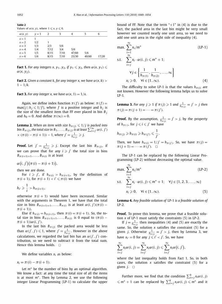
The meaning of α(x, y) is the minimum load of a bin Bwith items of size at least 1/x packed when an item ofsize 1/y cannot fit in bin B . Table 2 is from [6].

By the definition of α(x, y), it is not difficult to see thefollowing lemmas hold.

1052 X. Han et al. / Information Processing Letters 110 (2010) 1049–1054

Table 2Values of α(x, y), where 1 � x, y � 6.

α(x, y) y = 1 2 3 4 5 6

x = 1 1x = 2 1/2 1x = 3 1/3 2/3 5/6x = 4 1/4 7/12 3/4 5/6x = 5 1/5 8/15 7/10 47/60 5/6x = 6 1/6 8/15 7/10 23/30 49/60 17/20

Fact 1. For any integers x, y1, y2 , if y1 � y2 , then α(x, y1) �α(x, y2).

Fact 2. Given a constant k, for any integer x, we have α(x,k) >

1 − 1/k.

Fact 3. For any integer x, we have α(x,1) = 1/x.

Again, we define index function π( f ) as below: π( f ) =max{ j | h j � 1/ f }, where f is a positive integer and h j isthe size of the smallest item that FF ever placed in bin B jand h0 = 0. And define π(∞) = 0.

Lemma 2. When an item with size hπ( j) � 1/ j is packed intobin Bπ( j) , the total size in B1, . . . , Bπ( j) is at least

∑∞i= j′ α(i, j′)

× (π(i) − π(i + 1)) − 1, where j′ = 1hπ( j)

� j.

Proof. Let j′ = 1hπ( j)

� j. Except the last bin Bπ( j) , if

we can prove that for any i � j′ the total size in binsBπ(i+1)+1, . . . , Bπ(i) is at least

α(i, j′

)(π(i) − π(i + 1)

),

then we are done.For i � j′ , if hπ(i) > hπ(i+1) , by the definition of

π(i + 1), for π(i + 1) < i′ � π(i) we have

hi′ � 1

i> hπ(i+1),

otherwise π(i + 1) would have been increased. Similarwith the arguments in Theorem 1, we have that the totalsize in bins Bπ(i+1)+1, . . . , Bπ(i) is at least α(i, j′)(π(i) −π(i + 1)).

Else if hπ(i) = hπ(i+1) , then π(i) = π(i + 1). So, the to-tal size in bins Bπ(i+1)+1, . . . , Bπ(i) is 0 equal to (π(i) −π(i + 1))α(i, j′).

In the last bin Bπ( j) the packed area would be lessthan α( j′, j′) � 1, where j′ = 1

hπ( j). However in the above

calculations, we regarded the last bin has an α( j′, j′) con-tribution, so we need to subtract it from the total sum.Hence this lemma holds. �

We define variables xi as below:

xi = π(i) − π(i + 1).

Let m∗ be the number of bins by an optimal algorithm.We know a fact: at any time the total size of all the itemsis at most m∗ . Then by Lemma 2, we use the followinginteger Linear Programming (LP-1) to calculate the upper

bound of FF. Note that the term “+1” in (4) is due to thefact, the packed area in the last bin might be very smallhowever we counted nearly one unit area, so we need toadd one unit area in the right side of inequality (4).

max.∞∑

i=1

xi/m∗ (LP-1)

s.t.∞∑

i= j

xi · α(i, j) � m∗ + 1;

∀ j ∈{

1

hπ(1)

,1

hπ(2)

, . . . ,∞}

xi � 0, ∀i ∈ [1..∞). (4)

The difficulty to solve LP-1 is that the values hπ(i) arenot known. However the following lemma helps us to solveLP-1.

Lemma 3. For any j � 1 if π( j) � 1 and 1hπ( j)

= j′ > j then

π( j) = π( j + 1) = · · · = π( j′).

Proof. By the assumption, 1hπ( j)

= j′ > j, by the property

of hπ(·) , for j � i � j′ we have

hπ( j) � hπ(i) � hπ( j′) � 1

j′.

Then, we have hπ(i) = 1/ j′ = hπ( j′) . So, we have π( j) =π( j + 1) = · · · = π( j′). �

The LP-1 can be replaced by the following Linear Pro-gramming (LP-2) without decreasing the optimal value.

max.∞∑

i=1

xi/m∗ (LP-2)

s.t.∞∑

i= j

xi · α(i, j) � m∗ + 1; ∀ j ∈ {1,2,3, . . . ,∞}

xi � 0, ∀i ∈ [1..∞). (5)

Lemma 4. Any feasible solution of LP-1 is a feasible solution ofLP-2.

Proof. To prove this lemma, we prove that a feasible solu-tion x of LP-1 must satisfy the constraints (5) in LP-2.

If j = 1hπ( j)

then inequalities (4) and (5) are exactly the

same. So, the solution x satisfies the constraint (5) for agiven j. Otherwise 1

hπ( j)= j′ > j, then by Lemma 3, we

have xi′ = 0 for any j � i′ < j′ . So, we have

∞∑i= j

xiα(i, j) =∞∑

i= j′xiα(i, j) �

∞∑i= j′

xiα(i, j′

),

where the last inequality holds from Fact 1. So, in bothcases, the solution x satisfies the constraint (5) for agiven j. �

Further more, we find that the condition∑k

i= j xiα(i, j)

� m∗ + 1 can be replaced by∑k

i= j xiα(i, j) � m∗ and it

X. Han et al. / Information Processing Letters 110 (2010) 1049–1054 1053

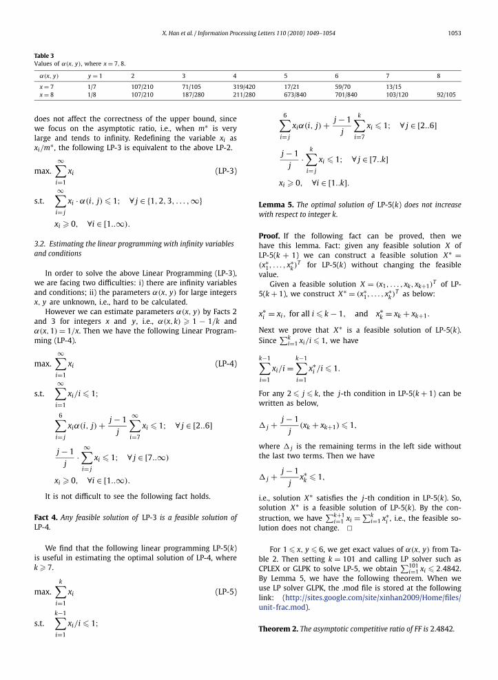
Table 3Values of α(x, y), where x = 7,8.

α(x, y) y = 1 2 3 4 5 6 7 8

x = 7 1/7 107/210 71/105 319/420 17/21 59/70 13/15x = 8 1/8 107/210 187/280 211/280 673/840 701/840 103/120 92/105

does not affect the correctness of the upper bound, sincewe focus on the asymptotic ratio, i.e., when m∗ is verylarge and tends to infinity. Redefining the variable xi asxi/m∗ , the following LP-3 is equivalent to the above LP-2.

max.∞∑

i=1

xi (LP-3)

s.t.∞∑

i= j

xi · α(i, j) � 1; ∀ j ∈ {1,2,3, . . . ,∞}

xi � 0, ∀i ∈ [1..∞).

3.2. Estimating the linear programming with infinity variablesand conditions

In order to solve the above Linear Programming (LP-3),we are facing two difficulties: i) there are infinity variablesand conditions; ii) the parameters α(x, y) for large integersx, y are unknown, i.e., hard to be calculated.

However we can estimate parameters α(x, y) by Facts 2and 3 for integers x and y, i.e., α(x,k) � 1 − 1/k andα(x,1) = 1/x. Then we have the following Linear Program-ming (LP-4).

max.∞∑

i=1

xi (LP-4)

s.t.∞∑

i=1

xi/i � 1;

6∑i= j

xiα(i, j) + j − 1

j

∞∑i=7

xi � 1; ∀ j ∈ [2..6]

j − 1

j·

∞∑i= j

xi � 1; ∀ j ∈ [7..∞)

xi � 0, ∀i ∈ [1..∞).

It is not difficult to see the following fact holds.

Fact 4. Any feasible solution of LP-3 is a feasible solution ofLP-4.

We find that the following linear programming LP-5(k)is useful in estimating the optimal solution of LP-4, wherek � 7.

max.k∑

i=1

xi (LP-5)

s.t.k−1∑

xi/i � 1;

i=1

6∑i= j

xiα(i, j) + j − 1

j

k∑i=7

xi � 1; ∀ j ∈ [2..6]

j − 1

j·

k∑i= j

xi � 1; ∀ j ∈ [7..k]

xi � 0, ∀i ∈ [1..k].

Lemma 5. The optimal solution of LP-5(k) does not increasewith respect to integer k.

Proof. If the following fact can be proved, then wehave this lemma. Fact: given any feasible solution X ofLP-5(k + 1) we can construct a feasible solution X∗ =(x∗

1, . . . , x∗k )T for LP-5(k) without changing the feasible

value.Given a feasible solution X = (x1, . . . , xk, xk+1)

T of LP-5(k + 1), we construct X∗ = (x∗

1, . . . , x∗k )T as below:

x∗i = xi, for all i � k − 1, and x∗

k = xk + xk+1.

Next we prove that X∗ is a feasible solution of LP-5(k).Since

∑ki=1 xi/i � 1, we have

k−1∑i=1

xi/i =k−1∑i=1

x∗i /i � 1.

For any 2 � j � k, the j-th condition in LP-5(k + 1) can bewritten as below,

� j + j − 1

j(xk + xk+1) � 1,

where � j is the remaining terms in the left side withoutthe last two terms. Then we have

� j + j − 1

jx∗

k � 1,

i.e., solution X∗ satisfies the j-th condition in LP-5(k). So,solution X∗ is a feasible solution of LP-5(k). By the con-struction, we have

∑k+1i=1 xi = ∑k

i=1 x∗i , i.e., the feasible so-

lution does not change. �For 1 � x, y � 6, we get exact values of α(x, y) from Ta-

ble 2. Then setting k = 101 and calling LP solver such asCPLEX or GLPK to solve LP-5, we obtain

∑101i=1 xi � 2.4842.

By Lemma 5, we have the following theorem. When weuse LP solver GLPK, the .mod file is stored at the followinglink: (http://sites.google.com/site/xinhan2009/Home/files/unit-frac.mod).

Theorem 2. The asymptotic competitive ratio of FF is 2.4842.

1054 X. Han et al. / Information Processing Letters 110 (2010) 1049–1054

Remarks. Similar with the proof in Lemma 5, we can seethat when k increases the ratio by LP-5 decreases. How-ever, the change is not significant. It seems it may bevery useful to get exact values for α(x, y), where x, y �7. But this does not work. Since we obtain exact valuesof α(x, y) for x, y = 7,8, aided by a programming (http://sites.google.com/site/xinhan2009/Home/files/alpha.c), thevalues are listed in Table 3. By the approach of solvingLP-5, we have that the competitive ratio of FF is 2.4838.So, it seems that it is very hard to get a much better resultthan 2.48 by our approach.

References

[1] J. Balogh, J. Békési, G. Galambos, G. Reinelt, Lower bound for theonline bin packing problem with restricted repacking, SIAM J. Com-put. 38 (1) (2008) 398–410.

[2] P. Barham, B. Dragovic, K. Fraser, S. Hand, T. Harris, A. Ho, R. Neuge-bauer, I. Pratt, A. Warfield, Xen and the art of virtualization, in: Pro-ceedings of the Nineteenth ACM Symposium on Operating SystemsPrinciples, Bolton Landing, NY, USA, October 19–22, 2003.

[3] A. Bar-Noy, R.E. Ladner, Windows scheduling problems for broadcastsystems, SIAM J. Comput. 32 (4) (2003) 1091–1113.

[4] A. Bar-Noy, R.E. Ladner, T. Tamir, Windows scheduling as a restrictedversion of bin packing, ACM Trans. Algorithms 3 (3) (2007) 28.

[5] A. Borodin, R. El-Yaniv, Online Computation and Competitive Analy-sis, Cambridge University Press, 1998.

[6] W.-T. Chan, T.-W. Lam, P.W.H. Wong, Dynamic bin packing of unitfractions items, Theoret. Comput. Sci. 409 (2008) 521–529.

[7] W.-T. Chan, P.W.H. Wong, On-line windows scheduling of temporaryitems, in: Proc. 15th Annual International Symposium on Algorithmsand Computation, ISAAC, 2004, pp. 259–270.

[8] W.-T. Chan, P.W.H. Wong, F.C.C. Yung, On dynamic bin packing: Animproved lower bound and resource augmentation analysis, Algorith-mica 53 (2) (2009) 172–206.

[9] E.G. Coffman Jr., M.R. Garey, D.S. Johnson, Dynamic bin packing, SIAMJ. Comput. 12 (2) (1983) 227–258.

[10] E.G. Coffman Jr., M. Garey, D. Johnson, Bin packing with divisible itemsizes, J. Complexity 3 (1987) 405–428.

[11] E.G. Coffman Jr., M.R. Garey, D.S. Johnson, Bin packing approximationalgorithms: A survey, in: D.S. Hochbaum (Ed.), Approximation Algo-rithms for NP-Hard Problems, PWS Publishing, 1996, pp. 46–93.

[12] J. Csirik, G.J. Woeginger, On-line packing and covering problems, in:On-line Algorithms The State of the Art, in: LNCS, vol. 1442, Springer-Verlag, 1996, pp. 147–177.

[13] Z. Ivkovic, E.L. Lloyd, Fully dynamic algorithms for bin packing: Being(mostly) myopic helps, SIAM J. Comput. 28 (2) (1998) 574–611.

[14] S.S. Seiden, On the online bin packing problem, J. ACM 49 (5) (2002)640–671.

[15] A. van Vliet, An improved lower bound for on-line bin packing algo-rithms, Inform. Process. Lett. 43 (5) (1992) 277–284.