Dynamic Changes in Determinants of Inequalities in Health ... › uploads › tx_sharepublications › ... · 3 1. Introduction Equality in health and health care is an important

Dynamic Changes in Determinants of

Inequalities in Health in Europe with a

Focus on Retirement:

Extended Results.

Jørgen T. Lauridsen, Terkel Christiansen and Astrid R. Vitved

Working Paper Series 44-2019

17 October 2019

1

Dynamic Changes in Determinants of Inequalities in Health in Europe with a Focus on Retirement:

Extended Results.

Jørgen T. Lauridsen1, Terkel Christiansen and Astrid R. Vitved

Department of Business and Economics, University of Southern Denmark,

Campusvej 55, DK-5230 Odense M, Denmark

E-mail: [email protected], [email protected] and [email protected]

Abstract:

Equity in health and health care is an important health policy objective in most European countries (OECD,

2013, 2017), and a number of empirical studies have shown the existence of inequities. Of particular interest

are the contributions to socioeconomic inequality in health from being retired because retirees most often

have lower income and lower health status relative to their working peers. Demographic changes in an ageing

society add further to the importance of investigating inequalities in health among the retired. Earlier studies

of health inequality across European countries have shown different results with respect to retirement status

as a determinant of health inequality. Furthermore, the development over time in this contribution, i.e., as

to whether it has increased or decreased, remains unexplored. Access to international comparative data from

European countries, however, allows comparative studies of the determinants of income-related inequalities

in a population’s health.

The present paper contributes to the literature on the association between retirement and income-related

health inequality by looking further into the contribution from three groups of retired individuals (younger

than 65 years; 65–74 years; 75 years and older) to income-related inequalities in health with focus on the

development in this contribution over time. The study is based on data from the first and the seventh waves

1 Corresponding author.

mailto:[email protected]



2

of the Survey of Health, Ageing and Retirement in Europe (SHARE), including individuals born in 1954 or

earlier (wave 1) and 1967 or earlier (wave 7) from 11 European countries (including Israel).

The results indicate that retirement status contributes to a varying degree to income-related inequality in

health across European countries, and that the variation can be related to income inequality as well as health

differences, depending on the country considered. Furthermore, it is indicated that the contribution from

retirement status changes in different patterns across countries, as it drops for some and increases for other

while being inconclusive for other.

JEL Classifications: I14, J26

Key Words: Health inequality, retirement, SHARE data.

Aknowledgement:

The SHARE data collection has been funded by the European Commission through FP5 (QLK6-CT-2001-

00360), FP6 (SHARE-I3: RII-CT-2006-062193, COMPARE: CIT5-CT-2005-028857, SHARELIFE: CIT4-CT-2006-

028812), FP7 (SHARE-PREP: GA N°211909, SHARE-LEAP: GA N°227822, SHARE M4: GA N°261982) and Horizon

2020 (SHARE-DEV3: GA N°676536, SERISS: GA N°654221) and by DG Employment, Social Affairs & Inclusion.

Additional funding from the German Ministry of Education and Research, the Max Planck Society for the

Advancement of Science, the U.S. National Institute on Aging (U01_AG09740-13S2, P01_AG005842,

P01_AG08291, P30_AG12815, R21_AG025169, Y1-AG-4553-01, IAG_BSR06-11, OGHA_04-064,

HHSN271201300071C) and from various national funding sources is gratefully acknowledged (see

www.share-project.org).

3

1. Introduction

Equality in health and health care is an important health policy objective in most European countries (van

Doorslaer et al., 1993), and a long list of empirical studies have shown the existence of inequalities. Of

particular interest has been the income-related inequality. Thus, income-related inequality in self-assessed

health was reported by van Doorslaer et al. (1993, 1997, 2003), based on the European Community

Household Panel (ECHP), (Eurostat, 1999). Access to international comparative data from European countries

allows a comparative study of determinants of income-related inequalities in health and contribution from

each factor. Of particular interest, due to the aforementioned earlier findings, are the contributions from

retirement. These contributions will be further elaborated on in what follows.

The aim of the present paper, which is an extended version of a forthcoming book chapter by Lauridsen et

al. (2019), is to add to what has been found regarding the association of retirement to health-related

inequality in health across European countries and the development in this contribution.

Following this introduction, Section 2 presents the data to be applied, i.e., SHARE wave 1 and 7. Next, Section

3 briefly outlines the quantitative methodology of the study, i.e., the concentration index and decomposition

approaches, followed by a presentation of results in Section 4. Finally, Section 5 rounds off with discussion

and concluding remarks.

2. Methods

Similar to the standard Lorenz curve, which shows how income concentrates across income classes, the

concentration curve (Figure 1) shows how health concentrates across income classes. The x-axis shows the

percentage of households, ranked by income, and the y-axis represents the corresponding share of

cumulated health.

4

Figure 1. The concentration curve and its decomposition into explained and non-explained inequality.

If health concentrates among the “wealthy” (i.e., those with relatively high income), then the curve locates

below the equity line. The concentration index (C) is calculated as twice the area between the curve and the

equity line (diagonal). Typically, a part of the inequality can be explained by socioeconomic and demographic

determinants (the shaded area), while another part remains unexplained (the white area).

When health is measured by a self-assessed health (SAH) scale with ordered categories, an ordinal scale is

obtained. This can be transformed to a cardinal scale by using a mapping method to scale the thresholds,

based on already known scores from another survey which has included both the SAH measure and an

instrument allowing a cardinal measure. Our approach is based the HUI-3 (Health Utility Index, version 3)

instrument that was included along with the SAH measure in a previous Canadian survey, National Population

Survey (NPS) (van Doorslaer et al., 1997; van Doorslaer and Jones, 2003). Throughout, we use the terms

“predicted health” and “health” synonymously.

Similar to previous studies initiated by van Doorslaer et al. (1993) we use the concentration index as our

measure of relative socioeconomic inequality in self-assessed health. The concentration curve ( )L s of Figure

1 plots the cumulative proportion of the population (ranked by socioeconomic status (SES), beginning with

lowest SES) against the cumulative proportion of health. A computational formula for C , which allows for

5

application of sample weights was given by Kakwani et al. (1997) as 1

21

N

i i i

i

C w y RN

, where

1

1 N

i i

i

w yN

is the weighted mean of (predicted) health, N the sample size, iy (predicted) health, iw

the sample weight of the individual (which sums to N ) and iR the fractional rank defined according to

Kakwani et al. as 1

1

1

2

ii

i j

j

wR w

N

, i.e. the weighted cumulative proportion of the population up to the

midpoint of each individual weight. Following the same authors, C can be conveniently computed as the

weighted covariance of iy and iR , i.e.

1

2 2 1cov ( , ) ( )( )

2

N

w i i i i i

i

C y R w y RN

.

A straightforward way of decomposing the predicted degree of inequality into contributions related to the

explanatory variables from the regression was proposed by Wagstaff et al. (2003). As motivated above, we

use an interval regression specification (Jones, 2000) for SAH, whereby the approach of Wagstaff et al. (2003)

implies a decomposition of the concentration index of predicted health as

(1) ˆˆ

k kk

k

xC C

,

where ̂ is the mean of predicted health , kx the mean of the determinant

kx , and kC the concentration

index of kx (defined analogously to C ).

In order to assess sampling variability and to obtain standard errors for the estimated quantities, the

contributions, i.e. the ˆ

k kk

xC

parts, cause troubles, as they are nonlinear functions of estimated

parameters. Therefore, we apply a “bootstrap” procedure (Efron and Tibshirani, 1993; Deaton, 1997) in a

five-step manner much similar to van Doorslaer and Koolman, (2004): First, the sample size is inflated to

allow for differences in sampling probability by dividing the sampling weights with the smallest weight and

rounding to nearest integer. Second, from this expanded sample a random sub-sample of the size of the

6

original sample is drawn with replacement. Third, the entire set of calculations as specified above are

performed on this sample. Fourth, this whole process is repeated 1,000 times, each leading to replicate

estimates. Fifth, using the obtained 1,000 replicates, standard deviations and t statistics can be computed.

As our focus is not on the magnitudes of the relationships between health and the determinants, we report

regression coefficients rather than marginal effects, given that the later implies a causal relationship that we

do not necessarily assume.

3. Data

The analyses in this paper have been conducted with data from the Survey of Health, Ageing and Retirement

in Europe (SHARE; Börsch-Supan et al., 2013), wave 1 of 2004-06 (Börsch-Supan, 2018) and wave 7 of 2017

(release 0) and thus covers individuals born in 1954 or earlier in Wave 1, or 1967 or earlier in Wave 7.

Table 1. Definition of variables Variable SHARE acronym Definition

Dependent variable:

SAH PH003_ (version 1) PH002_ (version 2)

Self-assessed health, 5 levels Version 1: Excellent, Very good, Good, Fair, Poor Version 2: Very good, Good, Fair, Bad, Very bad

Explanatory variables:

Income H017E, YRBIRTH, INT_YEAR

Income (real prices, PPP adjusted); OECD equivalized (OECD Social Policy Division)

Male 50-59 DN042_, YRBIRTH and INT_YEAR

Indicator for being male 50-59 year

Male 60-69 Indicator for being male 60-69 year

Male 70- Indicator for being male 70 year or more

Female 50-59 Indicator for being female 50-59 year

Female 60-69 Indicator for being female 60-69 year

Female 70- Indicator for being female 70 year or more

Employed or self-employed EP005_, YRBIRTH and INT_YEAR

Indicator for being employed or self-employed

unemployed Indicator for being unemployed

Houseworker Indicator for being houseworker

Disabled Indicator for being disabled

Retired -64 Indicator for being retired 64 year or less

Retired 65-74 Indicator for being retired 65-74 year

Retired 75+ Indicator for being retired 75 year or more

Single DN014_ Indicator for being single

Secondary education ISCED1997_r Indicator for having secondary education (ISCED 1997 level 2,3,4)

Higher education Indicator for having higher education (ISCED (ISCED 1997 level 5,6)

Foreign DN004_ Indicator for being born in abroad country

SAH2 Indicator for being exerted to SAH version 2

Weights:

Weight CCIW_W1 / CCIW_W7 Weight used for weighting of calculations

7

A total of 11 countries, which entered both waves, were selected for the study: Austria, Germany, Sweden,

Spain, Italy, France, Denmark, Greece, Switzerland, Belgium and Israel.

The variables include health status and demographic and socio-economic variables. Table 1 shows the

variables used, together with SHARE acronym and definition; means of variables are reported in Appendix.

4. Results

In the following presentation of results, only subsets of calculated results related to retired are reported; the

full set of calculations are reported in Appendix.

Table 2. Selected results for Wave 1

AT DE SE ES IT FR DK GR CH BE IL

Mean of predicted health 0.819 0.790 0.858 0.775 0.782 0.804 0.847 0.826 0.878 0.833 0.776

�̂� for predicted health 0.005 0.029 0.020 0.016 0.020 0.019 0.024 0.022 0.009 0.010 0.032

Means:

RETIRED - 64 0.231 0.100 0.075 0.068 0.178 0.119 0.131 0.111 0.048 0.112 0.084

RETIRED 65-74 0.225 0.255 0.231 0.161 0.226 0.232 0.200 0.221 0.207 0.224 0.166

RETIRED 75+ 0.198 0.188 0.236 0.132 0.162 0.206 0.198 0.146 0.215 0.198 0.161

Regression coefficients:

RETIRED - 64 -0.056 -0.041 -0.118 -0.073 -0.032 -0.019 -0.093 -0.027 -0.022 -0.022 -0.022

RETIRED 65-74 -0.055 -0.039 -0.021 -0.039 -0.046 -0.013 -0.062 -0.036 -0.029 -0.033 -0.035

RETIRED 75+ -0.081 -0.099 -0.041 -0.073 -0.059 -0.065 -0.096 -0.070 -0.030 -0.045 -0.058

Concentration indices:

RETIRED - 64 0.111 0.001 -0.0700 0.182 0.162 0.067 0.010 0.173 -0.031 0.088 0.221

RETIRED 65-74 0.085 -0.109 -0.092 0.007 -0.042 -0.029 -0.263 -0.078 -0.055 -0.013 -0.009

RETIRED 75+ 0.001 -0.248 -0.398 -0.138 -0.149 -0.127 -0.474 -0.283 -0.225 -0.088 -0.063

Contributions (%):

RETIRED - 64 -36.50 -0.02 3.60 -7.20 -5.78 -1.01 -0.59 -2.77 0.41 -2.63 -1.71

RETIRED 65-74 -26.55 4.67 2.57 -0.36 2.68 0.59 16.30 3.35 4.22 1.15 0.21

RETIRED 75+ 0.05 19.73 22.01 10.68 8.90 11.04 45.09 15.71 18.10 9.64 2.41

Note. Significance at level 5% indicated by grey background.

8

Table 2 and 3 show calculations from Wave 1 and 7 of mean and concentration index for the outcome variable

(predicted health), together with regression coefficients, means, concentration indices and contributions for

the three indicators; Retired 64 or less, Retired 65-74 years and Retired 75 years and above.

In both tables, the positive concentration indices for predicted health (�̂�) show that health is higher for the

economically better off. These measures vary across countries: they are overall highest in Israel, Germany,

Denmark and Greece, and lowest in Austria, Switzerland and Belgium.

Table 3. Selected results for Wave 7


Mean of predicted health 0.760 0.712 0.802 0.704 0.737 0.747 0.817 0.772 0.829 0.773 0.756

�̂� for predicted health 0.028 0.050 0.034 0.029 0.029 0.027 0.026 0.027 0.015 0.022 0.052

Means:

RETIRED - 64 0.186 0.047 0.027 0.038 0.053 0.111 0.048 0.061 0.024 0.077 0.035

RETIRED 65-74 0.231 0.224 0.273 0.182 0.190 0.258 0.253 0.155 0.216 0.260 0.165

RETIRED 75+ 0.242 0.279 0.246 0.174 0.251 0.232 0.221 0.257 0.208 0.209 0.139

Regression coefficients:

RETIRED - 64 -0.064 -0.058 -0.117 -0.020 -0.018 -0.018 -0.137 -0.018 0.026 -0.019 -0.028

RETIRED 65-74 -0.060 -0.024 -0.054 -0.044 -0.032 -0.059 -0.040 -0.032 -0.019 -0.015 -0.027

RETIRED 75+ -0.094 -0.032 -0.097 -0.106 -0.085 -0.092 -0.085 -0.115 -0.043 -0.036 -0.075

Concentration indices:

RETIRED - 64 -0.017 -0.068 -0.077 0.144 0.168 0.153 0.075 0.282 0.005 0.082 0.282

RETIRED 65-74 -0.012 -0.035 -0.107 0.119 0.103 0.075 -0.194 0.141 -0.069 -0.062 0.006

RETIRED 75+ -0.100 -0.130 -0.418 -0.117 -0.138 -0.099 -0.439 -0.160 -0.170 -0.233 -0.086

Contributions (%):

RETIRED – 64 0.98 0.53 0.90 -0.53 -0.75 -1.50 -2.29 -1.55 0.03 -0.70 -0.71

RETIRED 65-74 0.81 0.54 5.87 -4.63 -2.88 -5.66 9.20 -3.39 2.41 1.44 -0.07

RETIRED 75+ 10.73 3.26 37.08 10.47 13.59 10.56 38.64 23.22 12.54 10.35 2.28

Change in % contribution Wave 1 to 7

RETIRED – 64 37.48 0.55 -2.70 6.67 5.03 -0.49 -1.69 1.22 -0.38 1.92 1.00

RETIRED 65-74 27.36 -4.13 3.30 -4.28 -5.56 -6.25 -7.11 -6.74 -1.81 0.30 -0.27

RETIRED 75+ 10.68 -16.47 15.08 -0.21 4.69 -0.49 -6.45 7.52 -5.57 0.72 -0.13


9

It appears from both tables that there is a substantial variation between countries in all four components of

Formula (1).

In Wave 1 (Table 2), a variation is seen in mean health with a range from 0.775 (ES) to 0.878 (CH). The retired

as share of the country-specific samples of the populations 50+ years varies between 41.1% (IL) and 65.4 %

(AT). In particular, the variation in retired less than 65 years is large, ranging from 4.8% of the sample (CH)

to 23.1% (AT). Likewise, the variation in regression coefficients is largest in the youngest group of retired,

ranging from – 0,022 (CH, BE, IL) to -0.188 (SE) indicating geographical differences in health of retired groups.

The variation in the concentration indices appear largest in the oldest group of retired, varying from -0.474

(DK) to 0.001 (AT), indicating geographical variation in income-related inequality in health.

In Wave 7 (Table 3), mean health has decreased from 0.817 in Wave 1 to 0.764 in Wave 2, and average health

has a range from 0.712 (DE) to 0.829 (CH). The decline appears comparable across countries. The youngest

retired as share of the samples has also declined ranging from 2.4% (CH) to 18.6% (AT), while the oldest group

of retired has increased in all countries except CH and IL. The variation in the regression coefficient is still

largest in the youngest group of retired, ranging from -0.137 (DK) to -0.019 (BE). The variation in the

concentration indices has decreased but it is still largest in the oldest group of retired, ranging from -0.439

(DK) to -0.086 (IL).

Turning to the contributions to health inequality from these determinants, it should be kept in mind (cf.

Formula 1) that a positive figure indicates that the determinant increases inequality, while a negative figure

indicates the opposite. Thus, for most countries, early retirement (below 65 years of age) reduces health

inequality. A possible explanation could be that the retired below 65 years are economically better off than

the employed population (as indicated by the positive concentration indices), while at the same time being

in worse health than these (as indicated by the negative regression coefficients for health). An exception is

10

Sweden, where a significantly positive contribution occurs, as the regression effect as well as the

concentration index are both negative.

Similarly, the contributions for normal age retirement (65-74 year) are for most countries positive, thus

indicating that this age group increases inequality in health. For these countries, the positive contribution

occurs from a combination of a negative regression coefficient and a negative concentration index indicating

that low income as well as ill-health concentrates in this group. An exception is represented by Austria, where

a negative contribution occurs due to a positive concentration index (i.e. the group is economically better off

than the employed).

Finally, for the older retirees (75 and above), the significant contributions are uniformly positive, caused by

negative regression coefficients and negative concentration indices, i.e., ill-health as well as low income

concentrates in this group. The magnitude of the contributions for this group is considerably larger than for

the group aged 65-74, thus indicating that the major contribution to inequality from retirement stems

predominantly from the elder (aged 75+) group and less from the younger (aged 65-74) group.

Table 3 shows that health is still distributed in favor of the economically better off. The concentration indices

vary across countries in a pattern much similar to what was found for Wave 1. However, for most countries,

the concentration indices have increased from Wave 1 to Wave 7, thus confirming that socioeconomic

inequality in health has increased over time.

The means of the three determinants, reflecting the proportions of the 50+ populations who are retired,

varies across countries in patterns similar to what was seen for Wave 1. However, in general, with Germany

as an exception, the proportion of retired below 65 years has fallen from Wave 1 to 7 in all countries. Turning

to the retired proportions aged 65-74, a pattern similar to Wave 1 is seen, with only modest increases or

decreases for most countries. Finally, the proportions retired aged 75+ seem to increase for all countries as

should be excepted, however not for Switzerland and Israel.

11

Turning to the contributions to inequality in health from the determinants, it is generally confirmed (although

with exceptions) that retired in the two older age groups contribute to increased inequality in health, while

the pattern is more mixed for the younger group under 65. Thus, for Spain, Italy, France, Denmark, Greece,

Belgium and Israel, retired below 65 years reduces health inequality by having a negative contribution. As in

wave 1, the reason for this appears to be that the retired below 65 are economically better off than the

employed population (as indicated by the positive concentration indices, cf. Formula 1), while at the same

time being in worse health than these (as indicated by the negative regression coefficients for health, cf.

Formula 1). For Austria, Germany and Sweden, significantly positive contribution occurs, as the regression

effect as well as the concentration index are both negative.

Similarly, it is seen for the retired (65-74 year) that the contributions are positive for several countries, thus

indicating that this age group increases inequality in health. For these countries, the positive contribution

occurs from a combination of a negative regression coefficient and a negative concentration index indicating

that low income as well as ill-health concentrates in this group. For other countries, negative contributions

occur due to the combination of a positive concentration index and a negative coefficient for health (i.e. the

group is economically better off but in less good health than the employed).

Next, for the elder retired (75 and above), the pattern from Wave 1 is confirmed, i.e. the age group

contributes to increased inequality in health, given a combination of negative regression coefficients and

negative concentration indices. Again, the magnitude of the contributions for this group is considerably larger

than for the group aged 65-74.

Finally, considering development from wave 1 to 7, a quite mixed pattern with increases and decreases is

seen. For Austria and to some extent Belgium, all three age groups have increased their contributions to

health inequality. The increase for Austria is caused by a shift in the sign of the concentration indices for

retirement for all three groups from positive to negative. For Denmark and to some extent France and

12

Belgium, all three age groups have decreased their contributions. The decrease for Denmark is especially

caused by increased concentration indices for all three groups, as the index for the group below 65 shifted

from zero to significantly positive, while the negative indices for the two elder groups have reduced in

magnitude. For Germany and to some extent Spain and Israel, a mixed pattern is found, as the contribution

to inequality has risen for the group below 65 and fallen for the two older groups. The increase for the group

below 65 in Germany is especially connected to an increase in the concentration index for this group from

zero to significantly negative, while the reductions for the elder groups are related to reductions in the

magnitude of their negative indices. An opposite pattern, with reduced contribution for the group below 65

and increased for the two elder groups, is found for Sweden. Turning next to Italy and Greece, the groups

below 65 and 75 and above have both increased their contribution to inequality, while the intermediate

group has reduced it.

5. Discussion and conclusion

While the index of income-related inequality in health merely provides a summary measure, it is possible by

means of the decomposition into contributing factors to get a deeper insight into measured inequality.

Compared to the analyses by van Doorslaer and Koolman (2004) we have further divided retired into three

age groups rather than two which allows a more precise analysis of the contributions to inequality by retired.

The reference group for retired is wage earners and self-employed, and our focus is on differences between

wage earners and retired in Europe. In general the contribution from retired to inequality in income-related

health varies very much between countries and between age groups. While this is related to three

determining factors as well as unobserved residual inequality, it is difficult to find a coherent pattern across

countries.

In contrast to the suggestions by van Doorslaer and Koolman (2004) however, we find that it is especially the

oldest among the retired who contribute to income-related inequality in health in most of the 11 European

13

countries included in this analysis in both waves. The different contribution from retired to the inequality

index across countries is to a large extent associated with different relative income levels by retired. This may

be ascribed to different pension schemes as well as possibilities or habits in various countries in having

supplementary income through jobs for retired.

As to international comparisons of self-reported health there has been documented to be large variations

across countries that to a certain extent may be due to differences in reporting style rather than health

(Jürges, 2007). Accordingly, e.g. Danes tend to overrate their health (compared to the average) while

Germans and people in Southern Europe tend to underrate. Whether this seemingly pattern affects the

“true” distribution of health or the measured inequality in health has still to be explored; the latter may be

affected if the over – or under reporting behaviour is related to socioeconomic status.

Given the careful effort behind the collection of SHARE data, including pre-test sampling, face-to-face

interviews etc., the validity of the data as well as of the results presented in this study are considered to be

extremely high.

Calculation of the Concentration index and decomposition of health (Wagstaff et al., 2003) has been subject

to discussion and suggestions for corrections. A review thereof can be found in van Doorslaer and van Ourti

(2011). We address some of these in the following.

Linearity of the relationship between the explanatory variables and health is an assumption, which is for

discussion. For the case of age and gender, this has been resolved by using age categories and interactions

between these and gender as suggested by van Doorslaer and Koolman (2004). For some variables, which

are coded as binary indicators, the matter is not relevant. However, it is an open discussion as to whether

income should enter in linear or some non-linear form (van Doorslaer and Koolman, 2004; van Doorslaer and

van Ourti, 2011).

14

Furthermore, exogeneity of the explanatory variables may be an issue. In particular, the relationship between

income and health has been much discussed, given that income may as well be formed by health. The issue

was discussed recently by Heckley et al. (2016), who suggested a new methodology which explicitly

addressed the endogeneity. Another suggestion has been to use education instead of income as measure of

socioeconomic status, given that education is formed relatively early in life and therefore to a less extent

affected by present health (Arendt and Lauridsen, 2008).

Yet another point regards the assumption that the determinants of health do not affect the rank. However,

this conflicts with CI being defined from the covariance between health and income rank. Originally, the CI

was suggested as a measure of univariate income distribution and later used by Wagstaff et al. (2003) and

later authors to describe the bivariate distribution between health and income. Erreygers and Kessels (2013)

discussed this problem in details and suggested different bivariate approaches. Later, Kessels and Erreygers

(2016) and Erreygers and Kessels (2017) considered the simultaneity between income and health by

introducing a Structural Equation Model (SEM) approach. Yet another approach has been to discard the CI

approach and use a multivariate structural model for “unfair health”, based on which the inequality in health

can be summarized in different ways (Fleurbaey and Schokkaert, 2009).

The present paper can be seen as a follow-up on the results that was shown in van Doorslaer and Koolman

(2004) and therefore we have used the same methods, including the original concentration index. We are

aware of suggested correction to the concentration index by Wagstaff (2005) and Erreygers (2009) but we

have kept the original method to facilitate comparisons of previous results with the results from the present

paper. Wagstaff showed that that the upper and lower bounds of a binary variable whose inequality is

investigated depend on the mean of this variable, while Erreygers showed that this is the case for any variable

with bounds. Thus, when a health variable has bounds, the concentration index will depend on the mean,

and comparisons between populations with different health means therefore become problematic.

15

In their decomposition Wagstaff et al. (2003) showed that the Concentration index can be decomposed into

a deterministic and a residual component defined by twice the covariance between the error term and the

rank variable (socio-economic status or income). As pointed out by Kessels and Erreygers (2016) the

introduction of a socioeconomic variable in the regression of health may create a problem because the

covariation between health and the error term will be zero or close to zero, implying that all or most of the

variation of the concentration index has been explained.

As stated above, we are also aware of recent developments of decomposition methods considering that

socio-economic inequality is bivariate by nature and measuring the correlation between the two variables,

health and socio-economic status (Erreygers and Kessels, 2013; Kessels and Erreygers, 2016; Erreygers and

Kessels, 2017). To these, Heckley et al. (2016) added a Recentered Influence Function (RIF) regression

approach, where a two-dimensional decomposition of determinants of health as well as of determinants of

the socio-economic variable (income in the present paper), together with a feed-back between these two,

was suggested. However, although a risk of overstating the inequality may be implied, we have kept the

original decomposition method of health alone for the same reason as above.

The choice of concentration index involves a value judgement as discussed by e.g. Allanson and Patrie (2013)

and Kjellson et al. (2015). Thus, a choice has to be made between absolute and relative measures (where the

calculations in the present paper are based on a relative index), and between measures of health or ill-health

in case the index has both a lower and an upper bound (where self-assessed health with a lower and upper

bound has been used in the present paper). As shown by van Doorslaer and Koolman (2000) and Clarke et al.

(2002), the choice of index can influence the ranking.

16

References

Allanson P, Paetrie D. 2013. On the choice of inequality measure for the longitudinal analysis of income-

related health inequalities. Health Economics 22:353-365.

Arendt J, Lauridsen J. 2008. Do risk factors explain more of the social gradient in self-reported health when

adjusting for baseline health? European Journal of Public Health 18: 131-137.

Börsch-Supan A. 2018. Survey of Health, Ageing and Retirement in Europe (SHARE) Wave 1. Release version:

6.1.0. SHARE-ERIC. Data set. DOI: 10.6103/SHARE.w1.611

Börsch-Supan A, Brandt M, Hunkler C, Kneip T, Korbmacher J, Malter F, Schaan B, Stuck S, Zuber S. 2013. Data

Resource Profile: The Survey of Health, Ageing and Retirement in Europe (SHARE). International Journal of

Epidemiology 42: 992-1001.

Clarke PM, Gerdtham U-G, Johannesson M, Bingefors K, Smith L. 2002. On the measurement of relative and

absolute incomwe-related inequality. Social Science & Medicine 55: 1923-1928.

Deaton A. 1997. The Analysis of Household Surveys: A Microeconometric Approach to Development Policy.

Baltimore: John Hopkins University Press.

Efron B, Tibshirani RJ. 1993. An Introduction to the Bootstrap. Chapman & Hall : London.

Erreygers G. 2009. Correcting the concentration index. Journal of Health Economics 28: 504-513.

Erreygers G, Kessels R. 2013. Regression-based decompositions of rankdependent indicators of

socioeconomic inequality of health. Health and Inequality 21: 227-259.

Erreygers G, Kessels R. 2017. Socioeconomic status and health: A new approach to the measurement of

bivariate inequality. International Journal of Environmental Research and Public Health 14: 673.

17

Eurostat. 1999. European Community Household Panel (ECHP),

http://ec.europa.eu/eurostat/web/microdata/european-community-household-panel

Fleurbaey M, Schokkaert E. 2009. Unfair inequalities in health and health care. Journal of Health Economics

28: 73-90.

Heckley G, Gerdtham U-G, Kjellson G. 2016. A general method for decomposing the causes of socioeconomic

inequality in health. Journal of Health Economics 48: 89-106.

Jones A. 2000. Health Econometrics. In : Handbook of Health Economics. Culyer AJ, Newhouse JP (eds).

Elsevier : Amsterdam.

Jürges H. 2007. True health versus response styles: Exploring cross country differences in self-reported

health. Health Economics 16: 163-178.

Kakwani N, Wagstaff A, van Doorslaer E. 1997. Socioeconomic inequalities in health : Measurement,

computation, and statistical inference. Journal of Econometrics 77: 87-103.

Kessels R, Erreygers G. 2016. Structural equation modeling for decomposing rank-dependent indicators of

socioeconomic inequality of health: an empirical study. Health Economics Review 6: 56.

Kjellson G, Gerdtham U-G, Petrie D. 2015. Lies, damned lies, and health inequality measurements.

Understanding the value judgement. Epidemiology 26: 673-680.

Lauridsen JT, Christiansen T, Vitved AR. 2019. Dynamic Changes in Determinants of Inequalities in Health in

Europe with a Focus on Retirement. In: Börsch-Supan A, Bristle J, Andersen-Ranberg K, Brugiavini A, Jusot F,

Litwin H, Weber G. (Eds.): Health and socioeconomic status over the life course: First results from SHARE

waves 6 and 7. Berlin/Boston: De Gruyter (in press).

http://ec.europa.eu/eurostat/web/microdata/european-community-household-panel

18

OECD. 2013. Pensions at a Glance 2013. http://www.oecd-ilibrary.org/finance-and-investment/pensions-at-

a-glance-2013/relative-incomes-of-the-over-65s-late-2000s_pension_glance-2013-graph13-en

OECD. 2017. Inequalities in health. Paris: OECD. http://www.oecd.org/health/inequalities-in-health.htm.

SHARE-project (2018). Research Data Center and Data Access. http://www.share-project.org/data-access-

documentation/research-data-center-data-access.html

van Doorslaer E, Jones A. 2003. The determinants of inequalities in self-reported health : validation of a new

approach to measurement. Journal of Health Economics 22: 61-87.

Van Doorslaer E, Koolman X. 2000. Income-related inequalities in health: some evidence from European

Community Household Panel. Equity II Project Working Paper #1, Erasmus University, Rotterdam.

van Doorslaer E, Koolman X. 2004. Explaining the differences in income-related health inequalities across

European countries. Health Economics 13: 609-628.

Van Doorslaer E, van Ourti T. 2011. Measuring inequality and inequity in health care. Ch 5 in: Glied S and

Smith PC (eds.), The Oxford Handbook of Health Economics, Oxford: Oxford University Press: 837-869

van Doorslaer E, Wagstaff A, Bleichrodt H. 1997. Income-related inequalities in health: Some international

comparisons. Journal of Health Economics 16: 93-112.

van Doorslaer E, Wagstaff A, Rutten F. 1993. Equity in the finance and delivery of health care. Oxford

University Press.

Wagstaff A. 2005. The bounds of the Concentration Index when the variable of interest is binary, with an

application to immunization inequality. Health Economics 14: 649-653.

http://www.oecd-ilibrary.org/finance-and-investment/pensions-at-a-glance-2013/relative-incomes-of-the-over-65s-late-2000s_pension_glance-2013-graph13-en

http://www.oecd-ilibrary.org/finance-and-investment/pensions-at-a-glance-2013/relative-incomes-of-the-over-65s-late-2000s_pension_glance-2013-graph13-en

http://www.share-project.org/data-access-documentation/research-data-center-data-access.html

http://www.share-project.org/data-access-documentation/research-data-center-data-access.html

19

Wagstaff A, van Doorslaer E, Watanabe N. 2003. On decomposing the causes of health sector inequalities

with an application to malnutrition in Vietnam. Journal of Econometrics 112: 207-223.

20

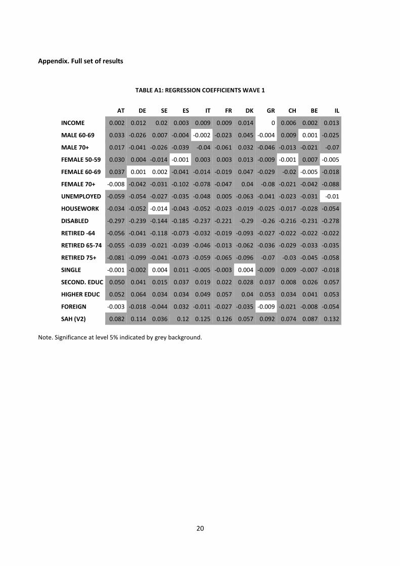
Appendix. Full set of results

TABLE A1: REGRESSION COEFFICIENTS WAVE 1


INCOME 0.002 0.012 0.02 0.003 0.009 0.009 0.014 0 0.006 0.002 0.013

MALE 60-69 0.033 -0.026 0.007 -0.004 -0.002 -0.023 0.045 -0.004 0.009 0.001 -0.025

MALE 70+ 0.017 -0.041 -0.026 -0.039 -0.04 -0.061 0.032 -0.046 -0.013 -0.021 -0.07

FEMALE 50-59 0.030 0.004 -0.014 -0.001 0.003 0.003 0.013 -0.009 -0.001 0.007 -0.005

FEMALE 60-69 0.037 0.001 0.002 -0.041 -0.014 -0.019 0.047 -0.029 -0.02 -0.005 -0.018

FEMALE 70+ -0.008 -0.042 -0.031 -0.102 -0.078 -0.047 0.04 -0.08 -0.021 -0.042 -0.088

UNEMPLOYED -0.059 -0.054 -0.027 -0.035 -0.048 0.005 -0.063 -0.041 -0.023 -0.031 -0.01

HOUSEWORK -0.034 -0.052 -0.014 -0.043 -0.052 -0.023 -0.019 -0.025 -0.017 -0.028 -0.054

DISABLED -0.297 -0.239 -0.144 -0.185 -0.237 -0.221 -0.29 -0.26 -0.216 -0.231 -0.278

RETIRED -64 -0.056 -0.041 -0.118 -0.073 -0.032 -0.019 -0.093 -0.027 -0.022 -0.022 -0.022

RETIRED 65-74 -0.055 -0.039 -0.021 -0.039 -0.046 -0.013 -0.062 -0.036 -0.029 -0.033 -0.035

RETIRED 75+ -0.081 -0.099 -0.041 -0.073 -0.059 -0.065 -0.096 -0.07 -0.03 -0.045 -0.058

SINGLE -0.001 -0.002 0.004 0.011 -0.005 -0.003 0.004 -0.009 0.009 -0.007 -0.018

SECOND. EDUC 0.050 0.041 0.015 0.037 0.019 0.022 0.028 0.037 0.008 0.026 0.057

HIGHER EDUC 0.052 0.064 0.034 0.034 0.049 0.057 0.04 0.053 0.034 0.041 0.053

FOREIGN -0.003 -0.018 -0.044 0.032 -0.011 -0.027 -0.035 -0.009 -0.021 -0.008 -0.054

SAH (V2) 0.082 0.114 0.036 0.12 0.125 0.126 0.057 0.092 0.074 0.087 0.132


21

TABLE A2. MEANS OF VARIABLES WAVE 1


PRED. HEALTH 0.819 0.79 0.858 0.775 0.782 0.804 0.847 0.826 0.878 0.833 0.776

INCOME 9.762 9.954 10.231 9.149 9.516 9.887 10.337 9.064 10.453 9.868 9.507

MALE 60-69 0.148 0.166 0.134 0.133 0.141 0.125 0.145 0.142 0.138 0.132 0.137

MALE 70+ 0.124 0.123 0.145 0.151 0.146 0.144 0.124 0.161 0.13 0.157 0.147

FEMALE 50-59 0.172 0.16 0.187 0.18 0.167 0.187 0.205 0.171 0.193 0.167 0.203

FEMALE 60-69 0.165 0.176 0.139 0.145 0.157 0.14 0.147 0.154 0.149 0.146 0.142

FEMALE 70+ 0.22 0.21 0.207 0.218 0.224 0.226 0.184 0.207 0.201 0.227 0.199

UNEMPLOYED 0.024 0.052 0.022 0.036 0.016 0.032 0.043 0.014 0.016 0.044 0.034

HOUSEWORK 0.12 0.1 0.01 0.323 0.216 0.113 0.017 0.242 0.082 0.16 0.133

DISABLED 0.017 0.028 0.027 0.044 0.011 0.024 0.033 0.015 0.032 0.041 0.069

RETIRED -64 0.231 0.1 0.075 0.068 0.178 0.119 0.131 0.111 0.048 0.112 0.084

RETIRED 65-74 0.225 0.255 0.231 0.161 0.226 0.232 0.2 0.221 0.207 0.224 0.166

RETIRED 75+ 0.198 0.188 0.236 0.132 0.162 0.206 0.198 0.146 0.215 0.198 0.161

SINGLE 0.408 0.364 0.365 0.327 0.342 0.339 0.37 0.319 0.312 0.299 0.257

SECOND. EDUC 0.479 0.553 0.255 0.083 0.176 0.27 0.44 0.22 0.387 0.25 0.346

HIGHER EDUC 0.194 0.256 0.205 0.091 0.055 0.182 0.306 0.138 0.081 0.241 0.228

FOREIGN 0.083 0.184 0.08 0.029 0.013 0.144 0.035 0.024 0.157 0.078 0.621

SAH (V2) 0.505 0.501 0.504 0.505 0.516 0.498 0.496 0.494 0.507 0.479 0.526

22

TABLE A3. CONCENTRATION INDICES WAVE 1


PRED. HEALTH 0.005 0.029 0.02 0.016 0.02 0.019 0.024 0.022 0.009 0.01 0.032

INCOME 0.061 0.05 0.034 0.064 0.055 0.046 0.039 0.054 0.055 0.055 0.063

MALE 60-69 0.192 0.056 0.161 0.083 0.106 0.014 0.106 0.182 0.159 0.056 0.045

MALE 70+ 0.115 -0.086 -0.168 -0.09 -0.097 -0.1 -0.35 -0.126 -0.078 -0.03 -0.006

FEMALE 50-59 -0.099 0.21 0.174 0.159 0.086 0.068 0.279 0.171 0.122 0.067 0.018

FEMALE 60-69 0.003 -0.062 0.046 -0.017 -0.014 -0.027 -0.05 -0.114 -0.1 -0.023 0.024

FEMALE 70+ -0.115 -0.324 -0.445 -0.259 -0.215 -0.153 -0.491 -0.341 -0.24 -0.155 -0.127

UNEMPLOYED -0.396 -0.172 -0.02 0.006 -0.257 -0.14 0.035 -0.21 -0.284 -0.12 -0.186

HOUSEWORK -0.221 -0.154 -0.406 -0.161 -0.239 -0.247 -0.348 -0.192 0.031 -0.169 -0.31

DISABLED -0.115 -0.318 0.058 -0.112 -0.302 -0.21 -0.281 -0.315 -0.007 -0.098 -0.359

RETIRED -64 0.111 0.001 -0.07 0.182 0.162 0.067 0.01 0.173 -0.031 0.088 0.221

RETIRED 65-74 0.085 -0.109 -0.092 0.007 -0.042 -0.029 -0.263 -0.078 -0.055 -0.013 -0.009

RETIRED 75+ 0.001 -0.248 -0.398 -0.138 -0.149 -0.127 -0.474 -0.283 -0.225 -0.088 -0.063

SINGLE -0.142 -0.228 -0.377 -0.196 -0.209 -0.168 -0.281 -0.184 -0.203 -0.146 -0.202

SECOND. EDUC 0.019 -0.011 0.1 0.257 0.309 0.106 0.026 0.216 0.043 0.055 0.057

HIGHER EDUC 0.165 0.268 0.305 0.405 0.498 0.383 0.274 0.474 0.403 0.202 0.227

FOREIGN 0.084 -0.125 -0.037 0.312 -0.021 -0.137 0.012 -0.159 -0.032 -0.066 -0.017

SAH (V2) 0.009 0.004 -0.001 -0.01 -0.006 0.003 0.011 0.011 -0.001 0.003 -0.002


23

TABLE A4. CONTRIBUTIONS WAVE 1


INCOME 24.193 25.863 41.762 12.493 29.529 25.651 27.749 -0.273 46.183 13.939 31.712

MALE 60-69 23.766 -1.021 0.89 -0.352 -0.233 -0.268 3.482 -0.534 2.463 0.083 -0.625

MALE 70+ 6.193 1.873 3.688 4.264 3.496 5.809 -7.042 5.022 1.659 1.175 0.233

FEMALE 50-59 -12.875 0.589 -2.633 -0.317 0.264 0.237 3.588 -1.375 -0.389 0.889 -0.078

FEMALE 60-69 0.441 0.001 0.081 0.828 0.196 0.474 -1.732 2.79 3.786 0.198 -0.248

FEMALE 70+ 5.415 12.329 16.706 46.262 23.332 10.694 -17.926 30.643 12.847 17.953 9.11

UNEMPLOYED 14.041 2.081 0.07 -0.062 1.226 -0.137 -0.466 0.649 1.321 2.037 0.245

HOUSEWORK 22.679 3.394 0.335 17.944 16.803 4.156 0.549 6.171 -0.53 9.231 9.174

DISABLED 14.69 9.035 -1.302 7.383 4.73 7.244 13.385 6.7 0.619 11.514 28.196

RETIRED -64 -36.499 -0.017 3.599 -7.202 -5.782 -1.007 -0.593 -2.772 0.408 -2.627 -1.707

RETIRED 65-74 -26.553 4.667 2.569 -0.356 2.681 0.591 16.302 3.354 4.22 1.146 0.207

RETIRED 75+ 0.05 19.734 22.007 10.681 8.895 11.044 45.088 15.708 18.104 9.635 2.411

SINGLE 1.639 0.819 -2.806 -5.442 2.309 1.136 -2.319 2.749 -7.337 3.865 3.82

SECOND. EDUC 11.429 -1.108 2.164 6.318 6.326 4.058 1.561 9.604 1.734 4.372 4.594

HIGHER EDUC 42.358 18.874 12.208 10.109 8.478 25.748 16.92 18.66 13.937 24.694 11.28

FOREIGN -0.505 1.811 0.752 2.328 0.02 3.451 -0.074 0.177 1.368 0.517 2.255

SAH (V2) 9.537 1.075 -0.089 -4.879 -2.269 1.117 1.526 2.726 -0.394 1.381 -0.579


24

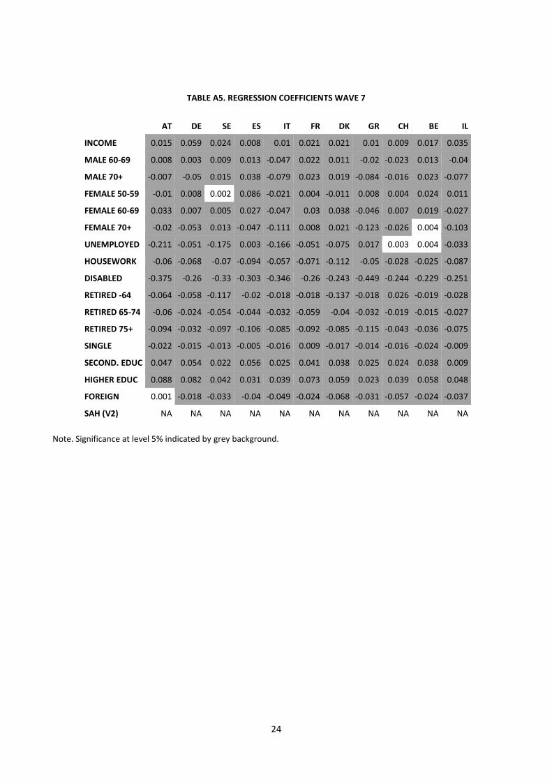
TABLE A5. REGRESSION COEFFICIENTS WAVE 7


INCOME 0.015 0.059 0.024 0.008 0.01 0.021 0.021 0.01 0.009 0.017 0.035

MALE 60-69 0.008 0.003 0.009 0.013 -0.047 0.022 0.011 -0.02 -0.023 0.013 -0.04

MALE 70+ -0.007 -0.05 0.015 0.038 -0.079 0.023 0.019 -0.084 -0.016 0.023 -0.077

FEMALE 50-59 -0.01 0.008 0.002 0.086 -0.021 0.004 -0.011 0.008 0.004 0.024 0.011

FEMALE 60-69 0.033 0.007 0.005 0.027 -0.047 0.03 0.038 -0.046 0.007 0.019 -0.027

FEMALE 70+ -0.02 -0.053 0.013 -0.047 -0.111 0.008 0.021 -0.123 -0.026 0.004 -0.103

UNEMPLOYED -0.211 -0.051 -0.175 0.003 -0.166 -0.051 -0.075 0.017 0.003 0.004 -0.033

HOUSEWORK -0.06 -0.068 -0.07 -0.094 -0.057 -0.071 -0.112 -0.05 -0.028 -0.025 -0.087

DISABLED -0.375 -0.26 -0.33 -0.303 -0.346 -0.26 -0.243 -0.449 -0.244 -0.229 -0.251

RETIRED -64 -0.064 -0.058 -0.117 -0.02 -0.018 -0.018 -0.137 -0.018 0.026 -0.019 -0.028

RETIRED 65-74 -0.06 -0.024 -0.054 -0.044 -0.032 -0.059 -0.04 -0.032 -0.019 -0.015 -0.027

RETIRED 75+ -0.094 -0.032 -0.097 -0.106 -0.085 -0.092 -0.085 -0.115 -0.043 -0.036 -0.075

SINGLE -0.022 -0.015 -0.013 -0.005 -0.016 0.009 -0.017 -0.014 -0.016 -0.024 -0.009

SECOND. EDUC 0.047 0.054 0.022 0.056 0.025 0.041 0.038 0.025 0.024 0.038 0.009

HIGHER EDUC 0.088 0.082 0.042 0.031 0.039 0.073 0.059 0.023 0.039 0.058 0.048

FOREIGN 0.001 -0.018 -0.033 -0.04 -0.049 -0.024 -0.068 -0.031 -0.057 -0.024 -0.037

SAH (V2) NA NA NA NA NA NA NA NA NA NA NA


25

TABLE A6. MEANS OF VARIABLES WAVE 7


PRED. HEALTH 0.76 0.712 0.802 0.704 0.737 0.747 0.817 0.772 0.829 0.773 0.756

INCOME 7.526 7.442 7.67 6.879 7.175 7.502 7.945 6.719 8.14 7.526 7.426

MALE 60-69 0.143 0.139 0.18 0.146 0.106 0.147 0.158 0.128 0.178 0.157 0.14

MALE 70+ 0.143 0.162 0.176 0.149 0.173 0.136 0.164 0.188 0.164 0.147 0.135

FEMALE 50-59 0.181 0.149 0.116 0.168 0.144 0.177 0.148 0.14 0.134 0.173 0.179

FEMALE 60-69 0.165 0.148 0.163 0.156 0.158 0.185 0.161 0.146 0.149 0.157 0.158

FEMALE 70+ 0.242 0.243 0.223 0.245 0.267 0.224 0.203 0.281 0.193 0.211 0.189

UNEMPLOYED 0.032 0.035 0.009 0.07 0.025 0.036 0.016 0.026 0.017 0.033 0.032

HOUSEWORK 0.058 0.042 0.001 0.236 0.179 0.038 0.008 0.222 0.056 0.056 0.128

DISABLED 0.007 0.042 0.031 0.067 0.026 0.031 0.034 0.026 0.027 0.067 0.114

RETIRED -64 0.186 0.047 0.027 0.038 0.053 0.111 0.048 0.061 0.024 0.077 0.035

RETIRED 65-74 0.231 0.224 0.273 0.182 0.19 0.258 0.253 0.155 0.216 0.26 0.165

RETIRED 75+ 0.242 0.279 0.246 0.174 0.251 0.232 0.221 0.257 0.208 0.209 0.139

SINGLE 0.483 0.444 0.447 0.34 0.343 0.445 0.418 0.394 0.394 0.416 0.3

SECOND. EDUC 0.629 0.68 0.486 0.341 0.539 0.486 0.486 0.377 0.759 0.486 0.398

HIGHER EDUC 0.264 0.305 0.361 0.132 0.074 0.268 0.435 0.201 0.165 0.383 0.397

FOREIGN 0.083 0.137 0.085 0.045 0.015 0.091 0.045 0.028 0.157 0.088 0.44


26

TABLE A7. CONCENTRATION INDICES WAVE 7


PRED. HEALTH 0.028 0.05 0.034 0.029 0.029 0.027 0.026 0.027 0.015 0.022 0.052

INCOME 0.048 0.043 0.043 0.051 0.056 0.049 0.045 0.06 0.053 0.036 0.05

MALE 60-69 0.101 0.142 0.177 0.283 0.098 0.153 0.184 0.146 0.166 0.085 0.153

MALE 70+ 0.066 0.053 -0.176 -0.065 -0.021 0.061 -0.298 -0.029 -0.04 -0.099 -0.084

FEMALE 50-59 -0.033 0.136 0.239 0.084 0.013 -0.044 0.312 0.132 0.023 0.131 0.008

FEMALE 60-69 0.058 -0.002 0.054 0.056 0.001 0.063 0.036 0.077 -0.018 -0.07 0.051

FEMALE 70+ -0.193 -0.233 -0.432 -0.227 -0.17 -0.123 -0.39 -0.222 -0.239 -0.262 -0.175

UNEMPLOYED -0.541 -0.707 -0.411 -0.445 -0.275 -0.318 -0.024 -0.713 -0.298 -0.318 0.117

HOUSEWORK -0.421 -0.142 0.006 -0.225 -0.293 -0.301 -0.164 -0.159 -0.187 -0.258 -0.339

DISABLED -0.166 -0.488 -0.326 -0.172 -0.395 -0.467 -0.173 -0.113 -0.358 -0.267 -0.477

RETIRED -64 -0.017 -0.068 -0.077 0.144 0.168 0.153 0.075 0.282 0.005 0.082 0.282

RETIRED 65-74 -0.012 -0.035 -0.107 0.119 0.103 0.075 -0.194 0.141 -0.069 -0.062 0.006

RETIRED 75+ -0.1 -0.13 -0.418 -0.117 -0.138 -0.099 -0.439 -0.16 -0.17 -0.233 -0.086

SINGLE -0.141 -0.2 -0.197 -0.069 -0.116 -0.155 -0.187 -0.095 -0.078 -0.175 -0.112

SECOND. EDUC -0.037 -0.118 -0.036 0.12 0.095 -0.026 -0.086 0.01 -0.031 -0.096 -0.001

HIGHER EDUC 0.247 0.298 0.26 0.36 0.379 0.333 0.197 0.368 0.337 0.273 0.22

FOREIGN -0.113 -0.15 0.027 -0.161 0.152 -0.089 -0.053 -0.104 -0.124 -0.013 -0.037



27

TABLE A8. CONTRIBUTIONS WAVE 7


INCOME 25.2 54.096 29.556 13.427 19.23 38.656 35.455 20.588 31.507 27.083 33.542

MALE 60-69 0.545 0.19 1.024 2.586 -2.229 2.441 1.544 -1.811 -5.556 0.999 -2.185

MALE 70+ -0.3 -1.197 -1.779 -1.773 1.337 0.957 -4.255 2.236 0.892 -1.995 2.232

FEMALE 50-59 0.275 0.459 0.234 5.84 -0.183 -0.137 -2.409 0.706 0.1 3.226 0.036

FEMALE 60-69 1.515 -0.006 0.155 1.153 0.005 1.771 1.033 -2.515 -0.147 -1.207 -0.551

FEMALE 70+ 4.485 8.439 -4.55 12.588 23.128 -1.088 -7.786 37.329 9.816 -1.183 8.665

UNEMPLOYED 17.537 3.525 2.312 -0.437 5.382 2.906 0.139 -1.52 -0.137 -0.226 -0.309

HOUSEWORK 6.964 1.129 -0.002 24.275 13.888 4.018 0.711 8.603 2.412 2.166 9.571

DISABLED 2.206 15.243 12.245 16.799 16.17 18.957 6.65 6.42 19.684 24.241 34.535

RETIRED -64 0.978 0.531 0.895 -0.534 -0.753 -1.496 -2.287 -1.551 0.026 -0.704 -0.709

RETIRED 65-74 0.805 0.536 5.865 -4.634 -2.877 -5.659 9.197 -3.39 2.408 1.441 -0.066

RETIRED 75+ 10.733 3.264 37.083 10.471 13.587 10.555 38.643 23.222 12.535 10.354 2.281

SINGLE 7.095 3.72 4.102 0.572 2.903 -3.031 6.362 2.527 4.009 10.232 0.794

SECOND. EDUC -5.077 -12.13 -1.442 11.045 5.848 -2.658 -7.397 0.465 -4.653 -10.352 -0.008

HIGHER EDUC 27.057 21.129 14.586 7.209 5.082 32.832 23.644 8.256 17.965 35.758 10.67

FOREIGN -0.015 1.072 -0.285 1.414 -0.517 0.977 0.756 0.434 9.139 0.167 1.503



28

TABLE A9. DEVELOPMENT OVER TIME: CHANGE IN CONTRIBUTIONS


INCOME 1.007 28.233 -12.206 0.934 -10.299 13.005 7.706 20.861 -14.676 13.144 1.83

MALE 60-69 -23.221 1.211 0.134 2.938 -1.997 2.709 -1.938 -1.277 -8.019 0.915 -1.56

MALE 70+ -6.493 -3.07 -5.467 -6.037 -2.159 -4.852 2.786 -2.786 -0.767 -3.17 1.999

FEMALE 50-59 13.15 -0.13 2.867 6.157 -0.446 -0.374 -5.997 2.081 0.489 2.338 0.114

FEMALE 60-69 1.073 -0.007 0.075 0.325 -0.19 1.297 2.765 -5.305 -3.933 -1.405 -0.303

FEMALE 70+ -0.931 -3.89 -21.255 -33.674 -0.204 -11.782 10.139 6.686 -3.031 -19.137 -0.445

UNEMPLOYED 3.496 1.444 2.242 -0.375 4.156 3.043 0.605 -2.169 -1.458 -2.264 -0.554

HOUSEWORK -15.716 -2.265 -0.336 6.331 -2.915 -0.138 0.162 2.432 2.942 -7.065 0.397

DISABLED -12.484 6.207 13.547 9.416 11.44 11.713 -6.735 -0.279 19.066 12.728 6.339

RETIRED -64 37.477 0.549 -2.704 6.667 5.029 -0.49 -1.694 1.221 -0.383 1.924 0.998

RETIRED 65-74 27.358 -4.131 3.295 -4.278 -5.558 -6.251 -7.105 -6.744 -1.812 0.295 -0.273

RETIRED 75+ 10.683 -16.471 15.076 -0.21 4.692 -0.489 -6.445 7.515 -5.569 0.719 -0.13

SINGLE 5.456 2.901 6.909 6.014 0.593 -4.168 8.681 -0.222 11.346 6.367 -3.027

SECOND. EDUC -16.507 -11.022 -3.606 4.727 -0.477 -6.715 -8.959 -9.139 -6.387 -14.723 -4.602

HIGHER EDUC -15.301 2.255 2.378 -2.9 -3.396 7.083 6.724 -10.405 4.027 11.064 -0.61

FOREIGN 0.49 -0.74 -1.037 -0.914 -0.537 -2.473 0.83 0.257 7.77 -0.351 -0.752



Documents

Dynamic Changes in Determinants of Inequalities in Health ... › uploads › tx_sharepublications › ... · 3 1. Introduction Equality in health and health care is an important