Dynamic Competition, Valuation, and Merger Activityfaculty.som.yale.edu/HeatherTookes/documents/7_Spiegel_Tookes_JF...THE JOURNAL OF FINANCE •VOL. LXVIII, NO. 1 FEBRUARY 2013 Dynamic

THE JOURNAL OF FINANCE • VOL. LXVIII, NO. 1 • FEBRUARY 2013

Dynamic Competition, Valuation, and MergerActivity

MATTHEW SPIEGEL and HEATHER TOOKES∗

ABSTRACT

We model the interactions between product market competition and investment valu-ation within a dynamic oligopoly. To our knowledge, the model is the first continuous-time corporate finance model in a multiple firm setting with heterogeneous products.The model is tractable and amenable to estimation. We use it to relate current in-dustry characteristics with firm value and financial decisions. Unlike most corporatefinance models, it produces predictions regarding parameter magnitudes as well theirsigns. Estimates of the model’s parameters indicate strong linkages between model-implied and actual values. The paper uses the estimated parameters to predict rivals’returns near merger announcements.

INTUITION AND FUNDAMENTAL MICROECONOMIC theory tell us that product mar-ket dynamics should have a significant impact on valuation and financial in-centives. Yet, directly testable models relating these issues have been largelyabsent from the corporate finance literature. This paper helps fill some of thesegaps by presenting a tractable framework for examining financial decision-making in a dynamic oligopoly with heterogeneous products. It shows that afirm’s competitive position can both profoundly influence its financial decisionsand impact how the firm is influenced by the decisions of others. The model’sexplicit closed-form solution allows one to estimate its parameters with ease.This paper takes advantage of this feature to apply the model to two financialquestions: (1) cross-sectional valuation and (2) a horizontal merger’s impacton rival firms. While other directly testable dynamic models (those that pro-duce quantitative as well as qualitative forecasts) have been relatively rarein the corporate finance literature, notable exceptions include Leland (1994,1998), Goldstein, Ju, and Leland (2001), Hennessy and Whited (2005, 2007),Strebulaev (2007), Schaefer and Strebulaev (2008), and Gorbenko and Strebu-laev (2010). However, to our knowledge, this paper is the first continuous-timecorporate finance model that takes place in a multiple firm setting with het-erogeneous products. The oligopoly setting allows us to derive predictions re-garding the interaction between a firm’s competitive position and how both itsown and its rivals’ decisions impact its immediate value and future responses.

∗Both authors are from the Yale School of Management. The authors thank Lauren Cohen,Engelbert Dockner, Alex Edmans, William Goetzmann, Alexander Gumbel, Jonathan Ingersoll,Uday Rajan, Raman Uppal, Ivo Welch, and seminar participants at the University of Toronto,UCSD, and the European Winter Finance Summit for their comments.

125

126 The Journal of Finance R©

This paper analyzes a differential game based upon a variant of theLanchester (1916) “battle” model. In the model n firms compete for marketshare (share of industry sales) by spending funds to acquire each other’s cus-tomers. The model’s continuous-time setting allows for closed-form solutionsthat would be very difficult to obtain in discrete time. The model’s dynamicstructure makes it straightforward to recover empirically unobservable pa-rameters such as consumer loyalty and firm-level spending effectiveness. Iden-tification in the model comes from market share evolution across firms and overtime. Using accounting and financial data, one can use the model to generateestimates of these parameters and make predictions regarding the variation infirm values both within and across industries.

Although the model has several appealing features, its mathematical struc-ture, which describes competition for market share, may not apply to all in-dustries. However, it seems unlikely that any one model can properly describeevery industry. The paper highlights the model’s empirical uses as well as limitsby first presenting estimates of the ease with which firms can acquire marketshare. The set of industries, firms, and years for which this is accomplishedis not exhaustive. For example, given that the model describes an oligopoly,industries with too many firms are excluded before attempting to generate es-timates. Nevertheless, they span a very broad array of 332 industries. While themodel’s structure inhibits it from accurately describing every existing industry,this limitation also opens up a way to see if the estimated parameters reflectactual economic forces or something else. This is done by comparing how themodel’s forecasts perform across industries where it should fit (mature indus-tries) with those where it should not (high growth industries). Our tests verifythat, relative to mature industries, the model’s empirical estimates for highgrowth industries are less accurate when it comes to valuing the underlyingfirms relative to mature ones.

In the model, there are several drivers of firm value, all of which impacta firm’s willingness to spend funds in an attempt to attract customers: con-sumer responsiveness (i.e., the ease with which a firm can steal consumersfrom rivals), firm level profitability per unit of market share, relative spendingeffectiveness, the number and capabilities of rival firms, industry growth, andthe discount rate. As an example of the model’s ability to generate quantita-tive as well as qualitative predictions, consider an innovation that increasesthe attractiveness of a firm’s product by 10%. Based on the model’s estimatedparameters, an investment of this type increases the value of the average firmin the malt beverages industry by 29.7%. In contrast, the same investmentin the line-haul railroad industry increases the value of the average firm byonly 15.5%. The difference is partially due to how willing consumers are toswitch brands in each industry, with it being relatively easier to lure away acompetitor’s customers in the malt beverage industry. Because of the model’sstructure, competitive responses of rivals to innovations are explicitly incor-porated in these estimates. In principle, these figures, and others like them,can be used to test the model in a valuation context. Under appropriate con-ditions, one can potentially compare the market’s immediate reaction to aninnovation’s revelation as well as the subsequent profitability and output of

Competition, Valuation, and Merger Activity 127

each competitor. In this way, the paper is related to the substantial empiricalliterature documenting intraindustry spillover effects near corporate events,including: initial public offerings (Hsu, Reed, and Rocholl (2010)); mergers andacquisitions (Eckbo (1983, 1992), Fee and Thomas (2004), and Shahrur (2005));dividend announcements (Laux, Starks, and Yoon (1998)); bankruptcies (Langand Stulz (1992)); corporate security offerings (Szewczyk (1992)); and cashpolicy (Fresard (2010)). The advantage of the model in this paper is that it pro-duces a testable structure for examining the cross-sectional variation in thesespillover effects.

One important financial application of the model is that it can be used as avaluation tool for firms operating in oligopolistic product markets. As a startingpoint, we test whether model-implied firm values capture actual values for over11,000 firm-year observations. This is done by taking parameters estimatedwith the model and then using them as inputs to the value functions derivedin the paper. While market shares alone can only explain approximately 20%of the variation in firm values, the model explains over 43%. The fit of themodel is driven by estimates of unobservable parameters such as industry-level consumer responsiveness, the company’s profitability, and the company’sability to attract customers.

The model is also capable of generating forecasts of each firm’s eventualmarket share and how long it will take to reach it. We use the model to project3- and 5-year-ahead changes in market shares and find correlations betweenactual and predicted changes in market shares of more than 0.08 and 0.15,respectively. These correlations are highly statistically significant. That themagnitudes of these correlations are substantially less than one suggests someof the limitations of the empirical implementation. However, as a benchmark,it is worth comparing the explanatory power of the model’s predicted changesin market share with other variables that have been used in the empiricalcorporate finance literature to describe the behavior of oligopolies (e.g., Eckbo(1983) and Shahrur (2005)). The three candidate variables that we examine areindustry concentration (HHI), change in HHI, and the (log) number of firms inthe industry. While these variables do offer additional explanatory power whenadded to the predictive market share regressions, the model-implied changesin market share remain statistically significant. Moreover, when we run a“horse race” among these variables using stepwise model selection based onthe Schwarz Bayesian Information Criterion, we find that the model-impliedchanges in market share ranks highest of the four candidate variables. When aversion of the model with stochastic market shares is applied to the empiricalimplementation, we find that the predictive power of the model is very robust.The market share prediction exercise in this paper is, to our knowledge, noveland may enhance current approaches to valuation.

The model’s flexibility allows it to be applied in many corporate financesettings.1 We present one example that revolves around a horizontal merger

1 There is a literature on finance and product market interactions. However, most models focuson the strategic implications of leverage (see, for example, Brander and Lewis (1986), Maksimovic(1988), Bolton and Scharfstein (1990), Hennessy and Livdan (2009), and the survey by Maksimovic


(M&A). In this setting, conflicting forces vie to determine the ultimate impacton rival firms. Rivals benefit from the reduced number of competitors. But theyare hurt if the combined firm is a much stronger competitor than were thestandalone firms. We take advantage of the structural model to disentanglethese two effects. The model also shows how mergers between one pair of rivalscan trigger profitable mergers among other pairs. This may prove useful infuture research on how merger waves start.

Estimates based on the M&A model indicate that it does help to explainthe cross-sectional pattern of rival returns in response to a horizontal merger.Regressing actual merger announcement period returns against the model’s(out of sample) forecast yields parameter estimates showing that a 1% changein the model’s return is associated with about a 1% change in actual returns.The R2 statistics are also quite reasonable for an exercise of this type, comingin at about 9%. Furthermore, this is accomplished by the model with the helpof only two data series: revenues and cost of goods sold. By comparison, thepurely empirical 11-variable model of customer and supplier returns in Feeand Thomas (2004) generates an R2 of 1.4% while Shahrur’s (2005) model ofrival returns, with 10 explanatory variables, generates an R2 of 9%. Theseanalyses fit observed returns using a variety of explanatory variables that arepotentially correlated with returns. Here the exercise is forward-looking. Ourforecasts are based on the estimated model parameters using only data thatwere available prior to the forecast date.

The model’s structure also allows one to decompose the effect of a merger onindustry rivals in ways that are impossible with a static model as guidance. Inparticular, it can be used to estimate the gain from a reduction in the numberof competitors versus the loss from facing a potentially stronger rival. Basedon the empirical estimates, if within-industry mergers did nothing but softencompetition through the reduction in the number of firms, then the medianrival’s value in our data would increase by about 2.52%. Similarly, if the onlyeffect was to generate a stronger competitor, the rivals would lose about 0.30%in value. This makes intuitive sense. Prior studies show that mergers createconsiderable value for the combining companies. Betton, Eckbo, and Thorburn(2008) report abnormal returns to the combined firm of more than 2%. Yet,studies going back to Eckbo (1983, 1992) also show that rival returns are small.The model reconciles these results by providing estimates of the two competingforces. It also shows that nonlinearities may matter. On average, the modelforecasts a rival return of 0.36%. (In actuality, firms in our database earn amean return of about 0.61% and a median return of 0.47%.) This comes from a2.22% gain due to the reduction in the number of firms in the industry, whichis partially wiped out by a 1.86% reduction in rival firm value, caused by thereduction in the number of competitors along with a new stronger firm. This

(1990)). On the empirical side of the literature, Chevalier (1995) and Leach, Moyen, and Yang (2006)provide evidence on the interaction between leverage and corporate behavior, but reach oppositeconclusions. It may be that as-yet unmodeled industry characteristics influence the degree to whichthe predictions in Brander and Lewis (1986) and Maksimovic (1988) are borne out in the data.


offsetting effect occurs because the reduction in the number of competitorsalong with the creation of a stronger rival creates an interaction effect thatworks to the newly created firm’s relative advantage.

The paper is organized as follows. Section I presents the basic model, in-cluding the solution to the infinite horizon case. Section II presents resultsfrom estimating key parameters in the model. Section III presents the M&Aapplication. Section IV concludes. Finally, the Appendix contains details on thederivation of the model’s equilibrium.

I. Basic Model

A. Players, Timing, Dynamics, and Strategies

The Lanchester (1916) battle model was originally designed to study militarystrategy. Since then variants have been widely used in the marketing literatureto examine advertising strategies (see, for example, Erickson (1992, 1997),Fruchter and Kalish (1997), Bass et al. (2005), Wang and Wu (2007); for areview, see Dockner et al. (2000)), although, to our knowledge, not in the formpresented here. This paper’s adaptation creates a differential game in whichcompetition among oligopolists selling heterogeneous goods can be explored.

Consider n risk-neutral value-maximizing firms battling for market share.Let ui(t) ≥ 0 represent the dollars spent by firm i on gaining market shareat instant t. Let si denote the effectiveness of spending. Note that spendingto acquire a competitor’s customers (ui) can imply a wide range of activities,including advertising, new product design, opening new stores, and R&D. Thesi parameters can represent the relative attractiveness of each firm’s productand/or the relative quality of its marketing campaigns.

The market share of firm i at time t is denoted by mi(t). Time is continuousand there is a finite starting point at t = 0. Given the initial condition mi(0), mievolves as follows:

dmi = φ[(1 − mi)uisi − mi

∑j �=i ujsj

]∑n

j=1 ujsjdt, (1)

where φ ≥ 0 represents the speed with which consumers react to each firm’sentreaties and can be interpreted as consumer disloyalty. (High values implyconsumers are easily lured away from one firm to another.) Intuitively, (1) saysthat the variation in firm i’s market share is simply the difference betweenwhat it gains from the market share held by its competitors and what it losesto them. For now, (1) is deterministic. Later, the analysis will generalize theequation to include a stochastic term. Equation (1) is the driving force behindthe model. According to equation (1), the market share of firm i increases withits own spending and effectiveness (ui and si, respectively) and decreases withthe spending and effectiveness of its competitors. Note that a high current mi(t)inplies that firm i has “more to lose” to its rivals and as a result it is easierfor competitors to gain market share. Thus, there are diminishing returns tobeing large.


Since this paper seeks to examine economic outcomes within industries thatare natural oligopolies, an assumption about consumer behavior is needed. Ifthe industry is characterized by positive network externalities then it is a nat-ural monopoly. In this case, once a firm’s market share reaches a tipping point,it eventually acquires all of the market. In a natural oligopoly such as theone described in this paper, however, that is not the case. Instead, it must bethat every firm has some consumers that find its offerings exceptionally attrac-tive even if most people use a rival’s products. For example, McDonald’s is thelargest fast food restaurant chain in the United States. Nevertheless, many con-sumers only eat at Burger King. Equation (1)’s structure captures this generalproperty: firms produce heterogeneous products and consumers have heteroge-neous preferences. This formulation also implies that there are diseconomiesof scale in spending to attract customers. Differentiating (1) shows that it ismonotonically decreasing in ui. Essentially, the first dollar a firm spends on itscustomer acquisition program does more to attract buyers than does the sec-ond, and so on. This is natural since customers that have a strong preferencefor a firm’s product line should be easy to bring in. As one moves further awayin preference space, the firm is then forced to spend even more to acquire newcustomers. For example, Burger King’s loyal customers will probably continueto eat there, no matter how much McDonald’s spends to attract them. On theother hand, the converse is true too—there are fans of McDonald’s that BurgerKing cannot attract.

Related to the issue of ensuring that the model describes an oligopoly is theassumption that spending effectiveness and actual dollars spent are multiplica-tive. That is, the relative value of a dollar spent by any two firms is constant.Other formulations like a power relationship, for example, usi

i , would alterthat. In this case, the relative value of each dollar spent would either increase(si > 1) or decrease (si < 0) with a firm’s own spending. In equilibrium, wesuspect that, with si < 1, the results would be qualitatively similar to whatthe current setting yields. But, of course, tractability would suffer. For si > 1,however, as spending increases the firm would become even more effective inattracting consumers. In the end, this would produce an industry with whatamount to network externalities and thus a natural monopoly.

The last element in equation (1) is φ. This is a consumer “stickiness” param-eter. High values imply that customers are easy to move in a short period oftime from one firm’s product line to another’s. Low values imply the opposite.Thus, one imagines that φ has a high value in the fast food industry since peo-ple purchase meals several times a day and purchases do not have to be maderepeatedly from the same firm. Conversely, it is likely that φ is low in industriesthat sell heavy equipment such as backhoes. These are durable goods that areonly replaced every few years. Furthermore, once a firm has committed itselfto a product line, it may be costly to switch vendors if the products interactwith each other.2

2 Further intuition can be garnered by looking at φ’s extreme values. Setting it to zero impliesconsumers never switch firms. The current market shares are thus forever frozen in place. At the


Before specifying the profit function, three additional observations from theformulation of dm (equation (1)) are worth noting. First, the discussion inthe paper assumes ui ≥ 0 in equilibrium. However, the equations are solvedunconstrained and in principle there exist exogenous parameter sets such thatone would need to solve a constrained problem instead. Since this paper focuseson mature stable industries, where exit is of secondary importance, it is usefulto restrict attention to cases in which the unconstrained equilibrium valuesof u are always strictly positive. Later, the sufficient exogenous parameterconditions needed to do this are laid out.

Second, dm is discontinuous whenever a firm “gives up” and sets its ui tozero. This is a result of the model’s assumption that it is relative spending thatmatters and ensures that the model is unit free. Beyond that, the dm equation’sbehavior when a firm sets ui = 0 also generates a particularly useful statistic,which we call the industry half-life. That is, if a competitor sets ui equal tozero, one can estimate the length of time it takes that firm to lose half of itscustomers when the other firms continue to compete for them.3

Third, the law of motion shown in equation (1) differs from the market-ing literature, which typically examines a duopoly model with either dm/dt =u1(1 − m) − u2m or dm/dt = u1

√1 − m− u2

√m (Dockner et al. (2000)). One ad-

vantage of using equation (1) instead is that it is unit free. This eliminates theproblem that changing the unit of currency also changes the rate at which mchanges over time. Another important advantage to this formulation is that rel-ative (rather than absolute) measures of spending are likely to be most relevantfor within-industry dynamics.

Returning to the model, instantaneous profits are assumed to be proportionalto market share and include a fixed operating cost. Let αi denote the revenuegenerating ability of firm i per unit of market share. Profits π equal revenuesminus both spending on market share competition and a fixed operatingcost fi:

πi(t) = egt (αimi(t) − ui(t) − fi). (2)

The term g represents the industry’s rate of growth. It is assumed that, asthe industry grows larger, profits and costs grow proportionately.4 Note thatspending by each firm does not impact the industry growth rate. Thus, themodel should be thought of as applying to an industry in which innovationstend to change customer loyalties rather than increase overall demand. Forexample, an easier-to-swallow aspirin will probably cause consumers to switch

other end, as φ goes to infinity, customers instantly switch vendors and do so en masse at the dropof a coupon.

3 Section I.C.1.b goes into greater detail and contains examples highlighting the half-life statis-tic’s implications while Section I.C.1.a contains estimates of its value. If one dislikes the model’sbehavior when ui equals zero, adding a fixed constant to equation (1)’s denominator will eliminateit. However, this comes at the cost of having a half-life without further assumptions.

4 In general for a starting value of π (0) in equation (2), multiply each equality by that amount.Since this has no impact on the model’s equilibrium conditions, the π (0) are suppressed to reducethe notational burden.


brands but seems unlikely to lead to an overall increase in pill consumption.One can modify the model to allow g to depend on ui but at the cost of a closed-form solution. We therefore leave g as an exogenous parameter making themodel better suited for an analysis of lower growth industries, as in the aspirinexample. Still, the model is quite flexible in its ability to describe differencesacross industries. If one thinks that it is easier to acquire market share infaster growing industries, this can be accommodated by simply setting φ toa larger value if g is larger. In terms of the mathematics it does not matterif market share growth comes from taking in newly entering consumers orstealing existing ones from rivals.

The profit function in equation (2) is similar to that used in many applica-tions, for example, the standard Cournot oligopoly model. Because profits arelinear in market share (sales), the firm’s production function exhibits constantvariable costs. At the same time, the fixed operating cost (fi) implies that thereare economies of scale. (If fi equals zero then total production costs are simplyproportional to sales. There is nothing in the model’s analysis that requires astrictly positive value of fi.) For many, although not all, industries these seemlike reasonable assumptions. For example, a fast food chain purchases rawmaterials (beef, potatoes, cleaning supplies, ovens, etc.) in a competitive envi-ronment. In cases like this, variable costs should be approximately proportionalto sales.

To help streamline the exposition, details regarding the derivation of themodel’s equilibrium conditions can be found in the Appendix. There we solve ageneral version of the model. The main text then employs the general solution todiscuss various special cases. Thus, in the main body of the paper, equilibriumconditions are simply stated without proof except for occasional references backto the Appendix.

B. The Equilibrium Value Functions

Let r denote the instantaneous discount rate. Assume that the discount rateexceeds the industry rate of growth (r > g). Define δ = r − g. Firms choose uito maximize expected discounted profits:

∫ ∞

0(αimi(τ ) − ui − fi) e−δτ dτ. (3)

Assume the parameters are such that no firm ever exits. Following standardpractice in the literature on differential games, the analysis seeks a Nashequilibrium in which the players use Markovian strategies (see Dockner et al.(2000)). The Appendix solves for the pure strategy equilibrium of this game andshows that each firm’s value function Vi at time t (i.e., the present discountedvalue of each firm’s profit stream conditional on the equilibrium strategies) can


be written as5

Vi (m, t) = ai + bimi (4)

within the scenarios considered in this paper.6 As shown in the Appendix,

ai = φαi[αisiz − (n − 1)]2

δ (φ + δ) (αisiz)2 − fiδ

(5)

and

bi = αi

φ + δ. (6)

In equation (5) above, z equals

z =n∑

j=1

1α jsj

(7)

and can be thought of as a measure of the competitive strength of firms withinan industry. Later on it will also be useful to define its mean as z = z/n. Intu-itively, a firm is a strong competitor if it can both profit from gaining marketshare (αj) and economically attract customers (sj). Since the units of measureare arbitrary (dollars or euros for α and some measure of effective marketing s)what matters is z, the ratio of one firm’s competitive strength relative to that ofeach rival. As a result, the term z appears repeatedly throughout the model’ssolution.

C. Equilibrium

C.1. Spending on Customer Acquisition and Retention

In the Appendix, we show that V ′i has as its solution αi/(φ + δ). Using the

definition of z and some algebra, one can show that

ui = αiφ(n − 1)[αisiz − (n − 1)](φ + δ)(αisiz)2 , (8)

which characterizes the equilibrium strategies that we seek. Observe that, ifthere are no fixed costs (fi = 0), equilibrium spending remains unchanged. Thisis because V ′

i is a function of only αi, φ, and δ.

5 We focus on pure strategies here. However, given the intuition that mixed strategies mightallow firms to collude to limit wasteful spending, we examined a two-firm version of the modelwith this property. In it, one firm receives an unanticipated (privately observed) positive shock toits profitability. In that setting, there exists an equilibrium in which spending on market shareacquisition does not increase to reflect the positive shock. In this equilibrium, both firms earn morethan they would in a full information environment.

6 There are, of course, boundary conditions under which the solutions given here will not hold.


Since the focus of this paper is on an ongoing oligopoly, we need to assumethe exogenous parameter values are such that no firm wishes to exit the indus-try. This naturally requires setting each firm’s fixed costs low enough that it isworth more if it operates than if it closes down. A sufficient condition to guar-antee this is to select fi small enough that (5) is strictly positive. However, thatwill only hold in the steady state if firms actually compete for market share andsufficiently weak firms will not. So long as a firm’s spending on market shareis strictly positive, the law of motion (1) guarantees a strictly positive marketshare along all possible paths. However, if spending (ui) is negative this neednot be the case. Thus, in keeping with this paper’s focus, assume every firm isstrong enough that αisizi − (n − 1) > 0.7

From equation (8), one can examine how competitive forces impact equi-librium spending. It is straightforward to show that spending is strictlyincreasing in consumer responsiveness, φ. When there is a greater incentive tospend money to attract customers, firms do so. Spending is strictly decreasingin the discount rate net of industry growth (δ) since it lowers the present valueof the revenue a new customer brings in. As one might expect, firms that earn agreater profit per sale (higher αi) spend more on customer acquisition becausethey are worth more to acquire. The derivative ∂ui/∂αi is positive as long asαisiz > 2 − 2/n. As noted above, if every firm in the industry is competing forcustomers, then αisizi > n − 1 and for n ≥ 2 this implies that αisizi > 2 −2/n as well. However, the impact of spending effectiveness (si) on equilibriumspending depends on a firm’s competitive strength. The derivative ∂ui/∂si ispositive as long as αisiz > 2(n − 1). Thus, if the firm is strong enough, highervalues of si will lead to higher ui, otherwise ui goes down.8 There are two forcesat work here. One is the standard trade-off. Firms with higher values of si canspend less and still attract customers. Weak firms find that the best option isto “split the difference” when si increases by reducing ui. For strong firms, thegain in market share from spending yet more on customer acquisition is justtoo strong to pass up for the offsetting gains a reduction in ui would bring. Butthere is a second factor at play that only becomes apparent in a multiple-firmmodel. When firms are relatively weak, increases in spending are met withmore aggressive spending by rivals, which decreases the incentives to spendmore. This can be seen by an examination of ∂ui/∂(α j �=isj �=i), which is alsopositive as long as αisiz > 2(n − 1). Comparative statics using equation (8) aresummarized in Table I.

7 Notice that as n goes to infinity the industry in this model becomes perfectly competitive. Forthe inequality to hold in the limit, one needs αisi z > 1 for each firm i. But this can only be trueif every “below average” firm is driven out, leaving a set of equally strong competitors. This, ofcourse, conforms to the usual microeconomic view of what should happen in such industries.

8 It is easy to generate examples in which there are firms in the industry for which the compar-ative static goes both ways. Consider an industry with four firms. Three have values of αisi = 1and one has a value equal to 2. In this case z = 3.5. For the low αisi firms, αisiz = 3.5 > 3 so theycompete for market share, but since αisiz = 3.5 < 6, for them ∂ui/∂si < 0. For the high αisi firm,αisiz = 7 > 6 so it has the opposite reaction relative to its weaker rivals, that is, ∂ui/∂si > 0.


Table IChange in the Equilibrium Spending ui from Equation (8)

Derivative withrespect to Economic Interpretation Sign Condition

φ The impact of an increase in consumer responsivenessincreases spending to acquire customers.

+ All firms

δ An increase in the discount rate reduces spending toacquire customers.

– All firms

αi The impact of an increase in firm profitability per unitmarket share on spending to acquire customers.

+ Large firms

si The impact of an increase in the attractiveness of a firm’sproducts on spending to acquire customers.

+ Large firms

(α j �=isj �=i) The impact of an increase in the competitive strength of arival on spending to acquire customers.

+ Large firms

C.1.a. Entry and Exit: Impact on Customer Acquisition and Value

With the model’s solution and restrictions on the exogenous parame-ter values in place, one can now analyze the equilibrium responses tochanges in z, the competitive environment. Since the paper’s empirical sec-tion examines the impact of a merger between rival firms, it is useful tobegin by seeing how a change in the number of competitors (n) alters equi-librium spending across firms. In a standard Cournot model, adding com-petitors decreases the equilibrium quantity produced by each firm. Firms“accommodate” the new entrant. Is the equivalent true here? Does addinga firm to the industry cause its competitors to reduce their spending oncustomer acquisition, with the incumbents all settling for smaller mar-ket shares? Because the model allows for heterogeneous firms this ques-tion cannot be answered until one first specifies what type of competitoris being added. A natural choice is to assume the new firm is “average” inthat it leaves z unchanged. Assuming this is the case, differentiating (8) leadsto the following proposition.

PROPOSITION 1: Increasing n while holding z constant leads to the followingspending change by firm i:

dui

dn= φ[nαisi z + 2(1 − n)]

n3(φ + δ)αi(si z)2 . (9)

This change in spending is strictly negative for average and below averagefirms (where αisi z ≤ 1) whenever n is greater than two. For these weak firms,increasing spending to attract customers in response to an increase in the num-ber of competitors is relatively futile. Stronger firms have larger values of αiand si and thus react differently from weaker firms. It is easy to show that firmsthat obtain more value per unit of market share (large αi) will spend more rel-ative to their less profitable rivals in response to entry (i.e., ∂2ui/∂n ∂ αi > 0).For firms that are particularly good at customer acquisition (high si) the


cross-derivative is ambiguous whereas for an average or below average com-petitor in the industry (i.e., αisi z ≤ 1) one can show it is strictly positive. Thus, ifthe model captures the competitive features of an industry, then looking acrosscompanies from weaker to stronger, the response to an increase in n should beincreasing in the data.

Compare the result in Proposition 1 to its analog within a standard homoge-nous product Cournot model. In a Cournot model, entry induces every firm toaccommodate the new firm by cutting back on production. Whether a firm isstrong or weak, it scales back on the control variable. In this paper, this isgenerally false for very strong firms. Empirically, this dichotomy may look like“predatory behavior” on the part of an industry’s leaders as these are the firmsmost likely to have large values of αi, si, and thus αisi z.

Based on the above results, intuitively one might now expect to find that verystrong firms actually gain market share if a new firm of average competitiveability enters the market. However, it turns out that this is not true. To beginthe analysis, the next proposition derives the steady state market share of eachfirm (mi) in terms of the model parameters.

PROPOSITION 2: The steady state market share of each firm equals

mi = 1 − n − 1αisinz

. (10)

Proof: Steady state occurs when mi is such that dmi/dt = 0, or

mi = uisi∑nj=1 uisi

. (11)

To generate (10) substitute (8) into (11). For the denominator of (11) this pro-duces

∑nj=1 ujsj = 1/z, after using z = ∑n

j=1 1/αisi. Some simple algebra thenyields (10). Q.E.D.

Two somewhat obvious empirical implications arise immediately from Propo-sition 2. The first is that in the steady state stronger competitors (those withhigher values of αisi) obtain a larger share of the market. Second, adding a newcompetitor of average competitive strength (thus leaving z unchanged) reducesthe market share of every firm.

A more interesting set of empirical predictions arises from a closer exami-nation of the model’s cross-sectional attributes. Proposition 1 shows that verystrong competitors increase their spending on market share acquisition in re-sponse to entry. Proposition 2, however, demonstrates that in the end they stilllose some customers. But the additional spending is not in vein. The increasedspending by stronger firms causes them to lose fewer customers than theirweaker rivals to the new entrant. Some minor algebra shows that the cross-derivative of a firm’s steady state market share to the number of competitorsand its own competitive ability (∂2mi/∂n∂(αisi)) is strictly positive. Thus, onehas the empirical hypothesis that, following the entry of a new firm into an


industry, weaker firms will lose a greater fraction of the market than strongerfirms. This happens even though the weaker firms begin with smaller fractionsof the market to begin with. Given their relative inability to compete effec-tively, their best response is to essentially cede market share and not fight toretain it.

C.1.b. Consumer Responsiveness and Corporate Values

Another variable impacting long-run industry values is the degree to whichconsumers respond to corporate entreaties (φ). Plugging mi into Vi yields firmi’s steady state value:

Vi(mi) = αi[αisiz − (n − 1)][(φ + δ)(αisiz) − φ(n − 1)]δ (φ + δ) (αisiz)2 − fi

δ. (12)

Differentiating (12) with respect to the consumer responsiveness parametershows that, in the steady state, firms are worth less if they are in an industryin which consumers are easily drawn away. The reason for this can be found inthe equilibrium values of ui and the fact that a firm’s steady state market share(mi) does not depend on φ. An examination of equilibrium spending to attractcustomers (equation (8)) shows that firms spend less if consumers become lessresponsive. Thus, every firm in an industry benefits from φ’s reduction becausethey earn the same steady state revenue stream while wasting fewer resourcestrying to lure away each other’s customers.

The effect of consumer responsiveness on corporate policy as outlined aboveis easily seen in real industries. For example, if beer drinkers exhibited greaterloyalty to particular brands, brewers would undoubtedly advertise less andcollectively earn higher profits. From 1981 to 2008, per capita beer consump-tion in the United States fell from 24.6 to 21.7 gallons despite heavy productadvertising (USDA, 2010). But no one brewer can reduce its own spendingwithout losing customers to competitors. Thus, in equilibrium, they end up ad-vertising just to retain their current market shares even amid stagnant sales.Compare this to the situation in, for example, natural gas distribution whereconsumers are locked into a single supplier and thus these firms do relativelylittle advertising.

Additional economic intuition can be gained by looking at what can be calledthe industry “half-life.” This represents the time it would take a firm to losehalf its customers if it stopped working to keep them by setting ui to zero. Thisvalue can be calculated from (1) and turns out to equal h = ln(2)/φ.

While the half-life (h) is the time that it would take a firm to lose half of itsmarket share if it stopped spending to attract customers, it can also be usedto analyze the growth of new firms. If a firm enters an industry, its rivals willnot passively let it grow. This slows the entrant’s growth, making it impossibleto capture half the market in the interval h described above. How long wouldit take? The model can be used to provide a quantitative answer. Plugging the


equilibrium values of ui into (1) yields

dmi

dt= φnαisi z − (n − 1)

nαisi z− φmi, (13)

which has a solution for mi(t) of

mi(t) = nαisi z − (n − 1)nαisi z

(1 − e−φt). (14)

Thus, the new entrant can be expected to capture a quarter of its steady statemarket share after t = h years. In this example, the incumbent firms’ reactionto the entrant cuts the entrant’s rate of growth in half.

Growing, newly public firms can be difficult to value, in part because ofchallenges associated with forecasting their future cash flows. Suppose theentrant in the above example goes public upon reaching a quarter of its steadystate market share. Again solving the ODE one finds that the entrant’s growthdecelerates from its pre-IPO levels. While the firm gained a quarter of its long-run market share in the first h years of its life, it will now take the same amountof time to go from one-quarter to three-eighths. What this means is that, if onecan estimate the value of h associated with a particular industry and eachfirm’s s and α, the model can be used to make predictions about each firm’slong-run market share, profitability, and spending on customer acquisition. Inaddition, it offers predictions about the time it takes new entrants to reachparticular market share levels. These estimates should also help predict cashflows and improve valuation in IPO studies.

C.2. Stochastic Market Shares

Prior to applying the model to real world data, it is useful to generalize thelaw of motion governing the change in market shares (equation (1)) to include astochastic component. This allows one to expand the interpretation of the errorterm in empirical work from that of measurement error alone to one that alsoincludes randomness in the underlying economy.

Since market shares always add to one, the structure of any error term mustnot pull them off of the unit simplex. At the same time, intuition suggests thatthere should exist a general symmetry in the error structure. For example, anatural restriction is that rearranging the order in which the firms are num-bered should have no economic impact. One way to do that is by starting withthe idea that competition in an industry is in some sense always bilateral. If acustomer of firm i randomly walks into firm j’s store, then i loses that customerto j. Thus, one can think of a random process governing the change in marketshares between two different firms i and j as ιi jσ

√mimjdwi j , where dwij is astandard Weiner process and ιij is an indicator variable that equals +1 if i < jand –1 if i > j. The indicator variable guarantees that a customer gained by onefirm is also a customer lost by another, thus ensuring that the market shareswill always add to one.


Each firm in an industry competes with n – 1 others. It therefore faces n – 1stochastic processes relating where its customers may arrive from or departto. Combined with the discussion above, the original law of motion describingfirm i’s market share formulated in equation (1) becomes:

dmi = φ[(1 − mi)uisi − mi

∑j �=i ujsj

]∑n

j=1 ujsjdt + σ

√mi

∑j �=i

ιi j√

mjdwi j . (15)

Using (15), the instantaneous variance for each firm’s market share isσ 2mi(1 − mi) and its covariance with firm j is −σ 2mimj . Overall then, thevariance–covariance matrix governing the change in market share can bewritten as

σ 2

⎡⎢⎢⎢⎢⎣

m1(1 − m1) −m1m2 · · · −m1mn

−m1m2 m2(1 − m2) · · · −m2mn

......

. . ....

−m1mn −m2mn · · · mn(1 − mn)

⎤⎥⎥⎥⎥⎦ . (16)

While adding a stochastic term to equation (1) induces uncertainty in thevalue of each firm going forward, it does not change the solution to its opti-mization problem. The solution to the original deterministic problem involvesa value function (V) that is linear in the state variable m. Thus, the second or-der term (∂2Vi/∂m2

i ), which interacts with the variance–covariance matrix (16),equals zero in the Hamilton–Jacobi–Bellman (HJB) equation for the new opti-mization problem. This implies that the solution to the deterministic problemis also the solution to the problem with stochastic elements.9

Even though adding stochastic terms leaves the solution to the control prob-lem unchanged, it does add new elements to the model’s properties. With theaddition of the Weiner processes, market shares no longer follow deterministicpaths and thus neither do firm values. Combining equations (4), (13), and (15)implies

dVi = αi

φ + δ

⎧⎨⎩[φnαisi z − (n − 1)

nαisi z− φmi

]dt + σ

√mi

∑j �=i

ιi j√

mjdwi j

⎫⎬⎭ . (17)

Thus, the instantaneous variance in Vi is proportional to that of mi.

II. Estimation

A. Outline

A primary goal in this paper is to incorporate market share dynamics re-sulting from product market competition into the analyses of firm valuation

9 A more extensive discussion of this general property relating when the deterministic andstochastic problems have identical solutions can be found in Section 8.2 of Dockner et al. (2000).


Table IIPossible Empirical Proxies for the Model’s Parameters

Parameter Description Possible Empirical Proxies

m Market share Share of total industrySalesAssets

u Spending to gain market Advertisingshare R&D

Capital expendituresCouponsLoyalty programs

φ, αsz Consumer responsivenessand relativecompetitive strength.

Estimation based on equation (1), usingequilibrium spending given in equation (8)and equilibrium market shares in equation(10) to obtain φ, mi , and αsz (see equation(19))

Estimation based on the discrete-time versionof equation (1) to obtain φ and

mi,t+1 − mi,t = φ( uisi (1−mi )−mi

∑Nj �=i uj sj∑N

j=1 uj sj

)Estimation of φ, α, and s based on equation (4)

α Revenue-generating Operating profitability Estimation based on equation (2) or (4)

f Costs of operations (fixed) Operating expenses (net of proxy for marketshare spending)

Estimation based on equation (2) or (4)

δ r – g: discount rate minus Industry cost of capitalindustry growth rate Industry growth rate

Estimation based on equation (4)

V Value of the firm Equity market capitalization + debt

and financial decision-making. One important advantage of the main model isthat it is well suited for empirical analysis. As Table II shows, several readilyavailable empirical proxies can be used. In this section, we take the first of thethree possible approaches to the estimation of φ that are suggested in Table II.Equation (1) provides a mechanism through which the consumer responsive-ness parameter φ can be estimated for each industry. Substituting equilibriumvalues of spending from equation (8) into equation (1) and using equation (11)to define steady state market share (mi) gives:

dm = φ(mi − mi(t))dt, (18)

which has a solution for mi(t) of:

mi(t) = mi + (mi(0) − mi)e−tφ. (19)

Because the stochastic component in (15) is white noise, albeit with a volatil-ity that depends on the vector of current market shares, equation (19) applies


regardless of whether the stochastic term is included in the dmi equation. Werely on equation (19) to estimate both φ and mi using nonlinear least squares.As described in more detail in Section I.B later, identification in the modelcomes from market share evolution across firms and over time.

Recall that φ captures consumer responsiveness, and is expected to begreater than zero. If consumers are unresponsive to spending, then theycontinue to purchase from their current firm no matter how much is spentto attract them. In estimation, the only restriction that we impose on φ isthat it is nonnegative and less than 25 (in our annual estimation, 25 wouldcorrespond to a customer half-life of just 10 days, implying extreme disloyalty).This rarely binds in the data. Recall from Proposition 2 that mi = 1 − n−1

αisinz .

Thus, parameter estimates from equation (19) also provide estimates of eachfirm i’s competitive strength, αisiz.

B. Identification

For each industry and year, we estimate the model using data from rolling10-year intervals and assume that φ remains constant over each interval.Since there are N firms and market shares have to add to one, there areN – 1 independent observations in each period. To ensure that annual mar-ket shares do not add to one, we eliminate the j smallest firms (i.e., thosewith t = 0 market shares of less than 3%, or the smallest firm in the in-dustry if there are no firms with market shares of less than 3%). There are10 years in the estimation window, and we therefore use 10(Nt – j) obser-vations to estimate the N – j+1 unknown parameters (mi for each of the n– j firms, plus φ). In reality, firms enter and exit industries, so there areactually 10(Nt – j) observations for each industry. Requiring t = 0 marketshares that are greater than 3% reduces noise in parameter estimates due tosmall firms moving in and out of the sample (because we focus on larger firmsthat are in the sample at the beginning of the estimation window). Assumingφ remains constant over the sample period, we estimate the parameters inequation (19) by minimizing the total sum of squared errors via nonlinear leastsquares.

Identification in the empirical estimation comes from changes in marketshare over time (to identify mi) and across firms (to identify φ). To illustratehow this is done, one can think of a two-step iterative process. The first stepstarts with initial values mi,0 from the data and a starting guess for the industryvalue of φ (we use one in the estimation). We then plug these into (19) to producea set of errors over time for each firm i. An initial estimate of mi is next producedby finding the value that minimizes the sum squares for firm i’s errors. Thisprocedure is then repeated across all firms in the industry to produce an initialvector of mi. Given a set of mi, the second step finds the industry value ofφ that minimizes the cross-sectional panel of squared errors in (19). Usingthe new φ as a starting value, this two-step process can be repeated untilconvergence is obtained for φ and all of the mi. In practice, the nonlinear leastsquares estimation of both φ and the m′

is is conducted simultaneously, using


an iterative process (Gauss–Newton method) and given starting values for allunknown parameters.

Given the estimated steady state market shares (mi) and Proposition 2,the firm-specific variable αisiz comes directly from the estimation describedabove. One benefit of the model and our estimation approach is that we donot need to estimate the firm-specific parameter s. This is because it is only afirm’s relative competitive strength (combined αisiz) that impacts equilibriumspending and value.

C. Data and Parameter Estimates

C.1. Data and Sample Selection

The only data required to estimate φ and mi are the market shares of allfirms in the industry. Market share, mi,t, is defined as firm i’s sales divided bythe sales of all U.S. headquartered CRSP/Compustat firms in the Compustatfour-digit SIC code during year t.10 We choose four-digit codes to mimic themodel’s industry setting as closely as possible. Compustat codes are used dueto findings in the literature (e.g., Guenther and Rosman (1994)) that linkagesamong firms based on these codes are higher than with CRSP SIC codes.

The initial sample consists of all firms for which there is nonmissing infor-mation on annual sales and all four-digit SIC industries in which there arefewer than 20 firms. The oligopolistic structure described in the main modelmakes industries with a large number of firms inappropriate in the context ofthis paper. We also exclude all industries with fewer than two publicly tradedfirms during the entire sample period. As noted earlier, we estimate the modelannually. Estimates for year t are obtained using rolling 10-year data inter-vals covering years t through year t + 9. We restrict our attention to firms forwhich we have data for more than 5 of the 10 years of each estimation interval.The estimation period begins in 1980 and ends in 2004.11 Given the model’sassumptions that r > g and that there is no entry or exit, we exclude industriesthat are growing (or shrinking) at very high rates. To do so, we impose the filterr > |g| where g is the average sales growth by all firms in the industry duringthe estimation window and r is the expected rate of return on the stock marketat the beginning of the estimation window.

The observations are pooled for each industry and then the industry- andfirm-specific parameters φ and αisiz, respectively, are estimated according to(19). For each 10-year rolling window, we also estimate firm-level parame-ters αi and fixed cost fi based on OLS estimation of a modified equation (2):πi(t) = egt(αimi(t) − ui(t) − fi). Rather than use proxies such as advertising or

10 The main model assumes no exit; however, due to changing product mix and SIC code re-classification for some firms, we adjust for “exit” in the data by assuming that each firm in theindustry gains market share from the exiting firm, in proportion to its current market share. Wedo not need to adjust for entry because data filtering requires that all firms be in the sample at thebeginning of rolling interval t.

11 Data for estimation are from 1980 to 2009. Estimates end in 2004, given the data requirementof greater than five annual observations in the estimation interval t through t + 9.


Table IIISummary of Estimated Parameter Values

This table presents summary statistics for the estimated parameter values for the 12,643 firm-yearobservations. Estimates for industry φ and firm miare based on nonlinear least squares estimationof equation (19), which is based on the law of motion for market share dm. Firm i’s market share,mi(t), is defined as the share of sales of all CRSP/Compustat firms in the industry. The initialsample consists of all four-digit SIC codes with fewer than 20 firms for the period 1980 through2009. Estimates are obtained for firms with market shares greater than 3%. Industries with r< |g| are excluded from the estimates. The individual firm profitability parameters (αi) per unitmarket share (millions of 2007 dollars per year) are estimated via OLS estimation of πi(t) =egt(αimi(t) − fi), where πi(t) = (Revenue – Cost of Goods Sold) and egt is the ratio of period t industrysales to industry sales in the first year of the sample.

φ mi αi

Mean 0.438 0.215 $2,020.025th Percentile 0.061 0.054 $138.8Median 0.192 0.132 $577.975th Percentile 0.548 0.305 $1,832.8Std. Dev. 0.630 0.231 $6,042

capital expenditures to capture spending to attract customers (which can varyin form substantially given our large cross-section of industries), we insteadlet πi(t) + egt ui(t) ≡ πi(t) = (Revenue – Cost of Goods Sold). This is equivalentto estimating prespending profitability (i.e., adding ui(t) back to both sides ofequation (2)). We explicitly subtract cost of goods sold from revenue in esti-mating prespending profitability (πi(t)) because this type of spending is tied tothe production of the good, not spending to attract customers (e.g., advertising,investments in PP&E, etc.). Importantly, the parameters of interest are of α

and f , which do not depend on the investment in market share, ui. Therefore,equation (2) becomes πi(t) = egt(αimi(t) − fi).12 For each firm, there are twounknown parameters: α, which multiplies market share, and fixed cost f (anintercept). To obtain estimates of these parameters, we need only one explana-tory variable, that is, market share (mit). Estimating αi and fi now simplyrequires estimation of the regression coefficient on current market share andthe intercept, respectively.

The egt term is calculated from industry sales. It equals the ratio of totalcurrent period industry sales to total industry sales in the first year of thesample (all values are in real 2007 dollars).

We obtain estimates for consumer responsiveness (φ), competitive strength(mi and αisiz), and profitability (αi) for 2,033 unique firms in 332 industries.There are a total of 12,643 valid firm-industry-year estimates, representingthe majority of the possible 14,678 firm-industry-year observations that meetthe initial data filtering requirements. Table III reports summary statisticson the estimated φ’s, mi, and αi. The mean (median) φ is 0.423 (0.191). Thiscorresponds to an industry half-life of about 1.6 (3.6) years. That is, it wouldtake a firm in the average industry 1.6 years to lose half of its customers

12 The variables φ and αit are constrained to be greater than or equal to zero, consistent withthe model.


if it completely stopped spending to acquire market share. The mean (me-dian) steady state market share of firm i is 19.0% (11.1%). These magnitudesfor mi are expected given that a minimum current market share of 3% isrequired for inclusion in the sample.13 Finally, the α parameter represents theannual profitability (in millions of 2007 U.S. dollars) per unit of market share.The mean (median) estimated α is $3,831.6 ($724.6) and is interpreted as theprofitability of a firm with 100% of all industry sales. While the summarystatistics in Table III provide a useful overview of the estimates, the discus-sion below highlights some potentially important between- and within-industryvariation.

C.1.a. Phi (φ) and Industry Half-Life Estimates

Table III reports estimated φ’s at the industry level along with half-lives(h) based on the point estimates for φ. The half-lives are expressed in years(calculated as ln(2)/φ). Individual φ’s, mi, and αi are estimated at the four-digitSIC code level; however Table IV shows the median φ within each two-digitlevel (for brevity). Despite the aggregation, useful observations can be madefrom the table.

Economically, the question is whether the half-lives in Table IV are “rea-sonable.” Recall that setting ui to zero does not imply that the firm ceasesoperations, maintenance, or customer service. Rather, it means that it doesnot actively compete for customers through things like advertising, R&D, andthe construction of new outlets. In this light the estimates seem plausible. Forexample, within the transportation industry, rail has a half-life of 4.9 years andair 2.1 years. Given the fixed nature of rail tracks, this difference is expected.While there are clearly some industries in Table IV with estimated half-livesthat appear to be either too high or too low, most seem to lie within the rangesone would expect.

We obtain parameter estimates for firms in all 332 industries at the four-digit level. For illustrative purposes, Table V presents firm-level estimates forfive of these industries for the year 2000 (the most recent year for which wehave full data for the year t to t + 9 estimation period). These industries re-flect significant between-industry variation in consumer responsiveness (φ of0.025 to 0.561), as well as within-industry variation in both steady state mar-ket shares and profitability of individual competitors. As in Table IV, manyof the estimates appear very plausible. For example, the estimated half-lifefor SIC Code 5731 (Radio, TV, and Consumer Electronics Stores) is 1.2 years,whereas the half-life for SIC code 3523 (Farm Machinery and Equipment) ismore than six times that number at 6.9 years. Here, the intuition is that modernstorefronts, aggressive advertising, or improvements to enhance the electronicsshopping experience will make customers more likely to patronize a given elec-tronics store. In contrast, consumers’ established comfort with the features of a

13 The current mean and median market shares of sample firms are 19.7% and 12.1%, respec-tively, which suggests modest future growth among larger firms in the industry.


Table IVEstimated Market Share Half-Lives by Two-Digit SIC Industry

This table presents estimated industry φ and market share half-lives, by two-digit SIC code usingdata for the years 1980 to 2009. The φ parameter is estimated for each four-digit SIC industryusing equation (19), which is based on the law of motion for market share dm. The estimatedvalues of φ and mi are chosen to minimize the sum of squared errors, εi. Each two-digit estimateis based on the median of the individual four-digit industry parameter estimates. Industries withmore than 20 firms or with r < |g| are excluded from the estimates. Individual firms’ steady statemarket shares, mi , are estimated but not reported. The half-lives listed use the point estimates forφ. Based on equation (1), the half-life (h) equals ln(2)/φ. This half-life represents, in years, the timeit would take a firm that spends nothing on customer recruiting to lose half its current marketshare.

SIC Code(Two-Digit) Industry φ Half-Life

1 Agricultural production crops 0.061 11.4537 Agricultural services 0.707 0.9818 Forestry 0.010 68.08710 Metal mining 0.236 2.94113 Oil and gas extraction 0.108 6.42514 Mining and quarrying of nonmetallic minerals, except fuels 0.264 2.63015 Building, construction, general contractors, and operative

builders0.365 1.898

16 Heavy construction other than building construction contractors 0.284 2.44417 Construction special trade contractors 0.414 1.67520 Food and kindred products 0.204 3.40321 Tobacco products 0.040 17.44122 Textile mill products 0.203 3.40823 Apparel and other finished products made from fabrics and

similar materials0.153 4.517

24 Lumber and wood products, except furniture 0.079 8.74525 Furniture and fixtures 0.176 3.93626 Paper and allied products 0.152 4.56127 Printing, publishing, and allied industries 0.097 7.17528 Chemicals and allied products 0.153 4.54229 Petroleum refining and related industries 0.154 4.51030 Rubber and miscellaneous plastics products 0.225 3.08731 Leather and leather products 0.122 5.69332 Stone, clay, glass, and concrete products 0.271 2.55933 Primary metal industries 0.171 4.05034 Fabricated metal products, except machinery and transportation

equipment0.241 2.876

35 Industrial and commercial machinery and computer equipment 0.183 3.79736 Electronic and other electrical equipment and components,

except computer equipment0.195 3.549

37 Transportation equipment 0.306 2.26538 Measuring, analyzing, and controlling instruments;

photographic, medical, and optical goods; watches and clocks0.201 3.457

39 Miscellaneous manufacturing industries 0.199 3.48440 Railroad transportation 0.143 4.86141 Local and suburban transit and interurban highway passenger

transportation0.087 7.975

(Continued)


Table IV—Continued

SIC Code(Two-Digit) Industry φ Half-Life

42 Motor freight transportation and warehousing 0.454 1.52844 Water transportation 0.565 1.22645 Transportation by air 0.457 1.51646 Pipelines, except natural gas 0.008 87.83347 Transportation services 0.146 4.73848 Communications 0.118 5.87949 Electric, gas, and sanitary services 0.141 4.90650 Wholesale trade-durable goods 0.222 3.12651 Wholesale trade-nondurable goods 0.226 3.06852 Building materials, hardware, garden supply, and mobile home

dealers0.085 8.202

53 General merchandise stores 0.076 9.08654 Food stores 0.373 1.85655 Automotive dealers and gasoline service stations 0.073 9.44856 Apparel and accessory stores 0.187 3.71557 Home furniture, furnishings, and equipment stores 0.122 5.70159 Miscellaneous retail 0.079 8.73860 Depository institutions 0.071 9.76561 Nondepository credit institutions 0.293 2.36362 Security and commodity brokers, dealers, exchanges, and

services0.316 2.193

63 Insurance carriers 0.122 5.69864 Insurance agents, brokers, and service 0.104 6.68365 Real estate 0.615 1.12767 Holding and other investment offices 0.279 2.48372 Personal services 0.146 4.76373 Business services 0.282 2.45675 Automotive repair, services, and parking 0.146 4.74276 Miscellaneous repair services 0.792 0.87678 Motion pictures 0.181 3.82979 Amusement and recreation services 0.170 4.08680 Health services 0.236 2.93482 Educational services 0.153 4.52583 Social services 0.420 1.64987 Engineering, accounting, research, management, and related

services0.580 1.195

99 Nonclassifiable establishments 0.104 6.685

particular brand of farm equipment and the delay between replacement cycleswill make them slower to switch brands in response to an improvement in,for example, tractor steering capabilities. This variation in consumer loyaltieswould seem to make these reasonable estimates. A data set containing the es-timated parameters shown in Table V for all firms and years in the sample isavailable in the Internet Appendix to this paper.14

14 The Internet Appendix is located on the Journal of Finance website at http:/www.afajof.org/supplements.asp.


Table VFirm and Industry Parameter Estimates for Selected Industries

This table presents parameter estimates at the individual firm level for a sample of five industriesfor the year 2000 (the last year in the sample for which we have full data for years t through t+ 9, used for estimation). The parameters φ, mi, and αisiz used to calculate model-implied V(m)are estimated via nonlinear least squares estimation of equation (19), which is based on the lawof motion for market share dm. Firm i’s steady state market share, mi,t, is defined as the shareof sales of all CRSP/Compustat firms in the industry. The individual firm profitability parameters(αi) are estimated via OLS, based on equation (2) in the text.

SIC Industry Name Company Est. φ φ s.e. Est. mi mi s.e. Est. α α s.e.

2082 Malt beverages AnheuserBusch

0.388 0.344 0.721 0.036 7,667.9 1,053.5

2082 Malt beverages Molson Coors 0.388 0.344 0.227 0.022 2,783.4 55.92731 Books: pubg, pubg

and printingMcGraw Hill

Corp0.276 0.134 0.391 0.013 2,190.3 143.1

2731 Books: pubg, pubg& printing

Readers DigestInc

0.276 0.134 0.149 0.014 3,142.7 847.8

2731 Books: pubg, pubgand printing

Scholastic Corp 0.276 0.134 0.150 0.007 1,587.49 563.6

3523 Farm machineryand equipment

Deere & Co 0.105 0.038 0.657 0.021 5,509.1 2,028.7


Toro Company 0.105 0.038 0.032 0.012 3,424.7 220.1


A G C O Corp 0.105 0.038 0.252 0.030 607.5 146.8

4011 Railroads,line-hauloperating

Union Pacific 0.025 0.002 0.163 0.024 17,418.5 4,936.0


BurlingtonNorthernSanta Fe

0.025 0.002 0.473 0.027 3,099.9 2,356.3


C S X 0.025 0.002 0.000 0.000 2,544.8 2,051.5

4011 Railroads,line-hauloperatng

NorfolkSouthern

0.025 0.002 0.215 0.020 23,578.6 5,867.6

5731 Radio, TV, conselect stores

RadioshackCorp

0.561 0.157 0.096 0.011 1,181.9 61.5


Circuit CityStores

0.561 0.157 0.211 0.012 686.9 63.5


Best Buy Co. 0.561 0.157 0.604 0.011 324.8 35.4

C.2. Calibration: Dynamics of Values and Market Shares

While the illustrative examples in Table V provide useful intuition, a naturalquestion to ask is whether the value functions described in equations (4)–(6)are consistent with observed firm value dynamics. We can use the parameterestimates obtained in the previous section to provide a more powerful test thanthe “reasonableness” checks above that we use as a starting point in evaluating


the validity of the model. We first calculate actual firm values, defined asequity market capitalization plus book values of debt at the end of year t. Theestimation procedure for the parameters φ, mi , and αi used to calculate model-implied V(m) is described in Section I.C.1. The final input to the value functionsis the cost of capital minus the growth rate (δ), which we define in two ways,using industry-level and market wide δ’s. Industry δIt is defined as the average(unlevered) cost of capital minus the average 5-year sales growth rate for allfirms in the four-digit SIC code. The market-wide δMt is defined as the long-run(1926 through period t) historical market risk premium plus the risk-free rateminus the long-run GDP growth rate.15 The market-wide measure capturesoverall equity market returns during our sample period.

Table VI presents results from regressing (log) actual firm values on the(log) model-implied V(m) from equations (4)–(6) using OLS and allowing forclustering of standard errors at the firm level. Because the regressions arelog–log regressions, the coefficients are interpreted as elasticities. Results froma benchmark regression of (log) actual firm values on market shares are alsogiven in Table VI, for comparison.

Panel A of Table VI contains the main results: model-implied V(m) capturesactual valuation. The coefficients on this variable are statistically significantand range from 0.497 to 0.583. Thus, a 1% increase in model-implied valuecorresponds to a 0.497% to 0.583% increase in actual firm value. This is tobe expected given that the model does not fit the data perfectly (the standardregression to the mean argument). However, it may also be due in part tothe market anticipating the news in accounting releases. For the model, anychange in an accounting variable is indeed “new news.” Market participants,though, may foresee such changes in values well in advance.16 The positiveintercepts in Panel A of Table VI are further evidence of this; market valuestend to rise over time for reasons outside the model and the data it employs.

Finally, note that the Table VI adjusted R2s in the regressions using V(m)alone are substantial. Their values range from 0.439 to 0.494 depending onthe definition of δ used. These are large compared to the R2 of 0.197 in thebenchmark case that uses market share as the sole explanatory variable. Here,again, the model seemingly brings to the data information beyond what astandard linear regression might.

The model assumes that r < g and also assumes no entry or exit. Because themodel is not intended to explain value dynamics in industries exhibiting rapid

15 The δ parameter is assumed to be positive in the model, but estimated δ’s are sometimes nega-tive. This can occur especially during high growth periods (for which the model is less appropriate).We exclude industry-years in which we observe negative values of δ. This reduces the sample sizeto 8,943 firm-year observations when industry-level δIt is used, and to 11,231 observations whenthe market-wide definition of δMt is used.

16 While not reported in the tables, this explanation is bolstered by the fact that, while the model-implied and actual market valuations are similar in magnitude across firms, the actual marketvalues are less volatile. The mean (log) actual value equals 6.92 (i.e., value of approximately $1billion) while the mean (log) model-implied value is 6.79 (i.e., value of approximately $890 million),a difference of only about 2%. In comparison, the actual market standard deviation is 1.83 whilethe model predicts a value of 2.23, a difference of about 18%.


Table VIPredicted Dynamics: Model-Implied V(m) and Actual Firm Values

The dependent variable is the (log) market value of the firm, defined as market capitalization ofequity plus book value of debt, in 2007 dollars, at the end of year t. The explanatory variables are(log) model-implied firm value (as specified in equations (4) through 6), industry growth and thefirm’s share of industry sales. The parameters φ, αisiz, αi, and fi used to calculate model-impliedV(m) are estimated via nonlinear least squares estimation of equation (19), which is based onthe law of motion for market share dm, and OLS estimation of the firm profitability equation,equation 2. The δt parameter is estimated in two ways: industry-by-industry, and a market-wideestimate. Industry δIt is defined as the average (unlevered) cost of capital, minus the average5-year sales growth rate for all firms in the four-digit SIC code. The market-wide δMt is defined asthe long-run (1926 through period t) historical market risk premium plus the risk-free rate minusthe long-run GDP growth rate. Market-wide δt is identical for all firms. Panel A contains resultsof estimating the model for the sample of stable industries (industries with r < |g| are excludedfrom the estimates). Panel B contains results of the sample selection validation exercise, in whichwe use all industries for which we are able to obtain estimates and introduce a lowgrowth dummyvariable equal to one if r < |g| and its interaction with V(m). We test the hypothesis that the modeldoes a better job estimating actual values for these industries. All firm-year observations of actualand predicted market values (Vit and V(mit)) are pooled and the model is estimated via OLS, withstandard errors clustered at the industry level.

Panel A: Model Implied V(m) and Actual Firm Values

V(m) Calculated Using V(m) Calculated UsingIndustry δIt Market-wide δMt

Intercept 5.932 2.311 2.436 6.038 2.936 3.043t-Value 51.38 11.16 11.68 57.33 13.13 14.08Market Share 3.773 1.646 3.818 1.779t-Value 17.03 8.27 18.48 8.75Model-Implied V(m) 0.583 0.519 0.570 0.497t-Value 22.89 17.51 19.22 14.91R2 (Adj) 0.197 0.494 0.525 0.197 0.439 0.474N 8,943 8,943 8,943 11,231 11,231 11,231

Panel B: Sample Selection Check

Intercept 5.084 3.517 3.456 5.382 3.911 3.799t-Value 51.29 15.39 15.65 51.48 17.43 17.74Market Share 3.312 2.116 3.111 1.879t-Value 15.32 9.63 15.81 9.55Model-Implied V(m) 0.367 0.3023 0.364 0.312t-Value 10.64 8.13 11.02 8.94Lowgrowth 0.848 –1.206 –1.020 0.656 –0.975 –0.757t-Value 6.72 –5.02 –4.29 6.05 –3.95 –3.20Lowgrowth × Share 0.461 –0.471 0.707 –0.100t-Value 1.67 –1.84 3.13 –0.47Lowgrowth × V(m) 0.217 0.217 0.207 0.184t-Value 6.14 5.47 5.98 4.96R2 (Adj) 0.241 0.474 0.510 0.219 0.421 0.457N 12,417 12,417 12,417 16,194 16,194 16,194


growth or contraction, the initial data filters exclude such industries from thesample. In order to check the validity of this filter, in Panel B of Table VI weallow high growth industries in the sample and introduce lowgrowth, a dummyvariable equal to one if the firm is in a stable industry (i.e., where r < |g|, as inthe Panel A regressions). We interact lowgrowth with V(m) and test the hypoth-esis that the model does a better job for the stable industries for which it wasintended. That is, we expect to observe a positive coefficient on the interactionbetween lowgrowth and V(m). This is exactly what we observe. While the modelis still important in explaining values of all firms, the estimated coefficient onV(m) drops relative to Panel A. The estimated coefficient on the interactionis around 0.21, implying that, for every 1% change in model-implied values,actual values increase 0.21% more for firms in stable industries than firms inless stable industries. This validates the initial sample selection criteria andalso suggests the types of industries for which the model does and does notperform well.

As mentioned previously, we define industries using four-digit SIC codes.While this is the finest level of SIC category, it is possible to examine evennarrower industry definitions based on other classification systems. To checkthat our main results are not driven by the choice of industry definition, wereestimate all parameters and the regressions shown in Table VI but replaceSIC codes with six-digit NAICS codes. Although we obtain estimates for asmaller set of firms using this industry definition, the main findings regardingthe ability of the model to explain actual firm valuations remain. Detailedresults are available in the Internet Appendix.

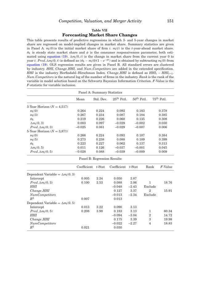
In addition to predictions about value, the model also provides clear predic-tions regarding the evolution of market shares within industries. Subtractingmi(0) from equation (19) yields mi(t) − mi(0) = (mi − mi(0))(1 − e−φt). Given ini-tial condition mi(0), we can use estimates from the model to forecast t-period-ahead changes in market share. We first use data from year t – 9 to year tto estimate the model’s parameters. We then use these estimates to generateout-of-sample predictions of changes in market shares from year t to years t +3 and t + 5. Table VII shows results from regressing actual 3- and 5-year-aheadchanges in market share on model-implied (predicted) changes for all firms andindustries for which we are able to obtain estimates. These results are based ondata from all the industries for which we have parameter estimates (i.e., thosein Panel A of Table VI). Because the estimates require data for the 10 yearsprior to the forecast period as well as the forecast period itself, the number ofobservations is substantially smaller than in Table VI. Still, there are 4,417observations in the 3-year-ahead regressions and 3,871 observations in the5-year-ahead regressions. Both sets of regressions show significant predictivepower of the model-implied changes in market share.

In the theory presented in this paper, the model-implied change in marketshare is the only relevant explanatory variable and hence is the only variablein the main predictive regression specification, shown in the leftmost columnsof Table VII. Further, the estimated coefficients on the model-implied changesin market share are 0.10 for 3-year-ahead changes and 0.21 for 5-year-ahead


Table VIIForecasting Market Share Changes

This table presents results of predictive regressions in which 3- and 5-year changes in marketshare are regressed on model-implied changes in market share. Summary statistics are givenin Panel A. mi(0) is the initial market share of firm i. mi(t) is the t-year-ahead market share.mi is steady state market share and φ is the consumer responsiveness parameter, both esti-mated using equation (19). �mi(0, t) is the change in market share from the current year 0 toyear t. Pred �mi(0, t) is defined as (mi − mi(0)(1 − e−φt) and is obtained by subtracting mi(0) fromequation (19). OLS regression results are given in Panel B. All standard errors are clusteredby industry. HHI, Change HHI, and Num Competitors are added in the extended specification.HHI is the industry Herfindahl–Hirschman Index. Change HHI is defined as HHIt – HHIt–1.Num Competitors is the natural log of the number of firms in the industry. Rank is the rank of thevariable in model selection based on the Schwartz Bayesian Information Criterion. F-Value is theF-statistic for variable inclusion.

Panel A: Summary Statistics

Mean Std. Dev. 25th Pctl. 50th Pctl. 75th Pctl.

3-Year Horizon (N = 4,517)mi(0) 0.264 0.224 0.092 0.183 0.378mi(3) 0.267 0.234 0.087 0.184 0.385mi 0.219 0.226 0.060 0.135 0.308�mi(0, 3) 0.003 0.097 –0.029 –0.002 0.030Pred �mi(0, 3) –0.025 0.081 –0.029 –0.007 0.006

5-Year Horizon (N = 3,871)mi(0) 0.266 0.224 0.093 0.187 0.384mi(5) 0.273 0.238 0.088 0.189 0.399mi 0.223 0.227 0.062 0.137 0.313�mi(0, 5) 0.011 0.126 –0.037 –0.001 0.045Pred �mi(0, 5) −0.028 0.088 –0.039 –0.009 0.009

Panel B: Regression Results

Coefficient t-Stat Coefficient t-Stat Rank F-Value

Dependent Variable = �mi(0, 3)Intercept 0.005 2.24 0.050 2.87Pred �mi(0, 3) 0.100 2.53 0.088 2.06 1 18.76HHI –0.048 –2.43 ExcludeChange HHI 0.127 3.37 2 15.91NumCompetitors –0.013 –2.34 ExcludeR2 0.007 0.013

Dependent Variable = �mi(0, 5)Intercept 0.013 3.22 0.090 3.13Pred �mi(0, 5) 0.208 3.98 0.183 3.13 1 60.34HHI –0.094 –3.04 2 14.72Change HHI 0.175 3.39 3 19.98NumCompetitors –0.022 –2.27 4 18.83R2 0.021 0.030


changes, with t-statistics greater than 2.5. Thus, the model not only capturesvariation in firm values, but also predicts within-industry market share dy-namics. As a benchmark, it is worth comparing the explanatory power of themodel’s predicted changes in market share (based, as previously noted, onlyon revenue and cost of goods sold (COGS)) to other variables that have beenused in intraindustry studies of returns near major events (e.g., Eckbo (1983),Shahrur (2005)). In the right-hand-side columns of Table VII, we introduceindustry concentration (HHI), change in HHI, and number of firms in theindustry as alternative explanatory variables. While these variables do offeradditional explanatory power when added to the regressions, the coefficientson the predicted changes in market share from the model remain statisticallysignificant. Moreover, when we run a horse race among these variables usingstepwise model selection based on the Schwarz Bayesian Information Crite-rion, we find that the model-implied changes in market share ranks highest ofthe four candidates in these out-of-sample predictive regressions.

The benchmark market share analysis in Table VII assumes that the worldis deterministic and that all errors in the estimation are due to measurementerror. In reality, industries are likely to be hit by random shocks. We use theframework presented in Section I.C.2 to explicitly account for stochastic shocksin the estimation of market share evolution. Rather than simply allowing forindustry clustering of standard errors as we do in Table VII, we introduce thestructure of the variance–covariance matrix defined in (16) to the empiricalimplementation. We do so two ways. In the first approach, we use OLS toobtain coefficient estimates and then use (16) and year t market shares toestimate standard errors (and industry-specific σi). In the second approach,given that we have information on market shares, we initially set all σi equalto those obtained using OLS and use year t market shares in (16) as a weightmatrix to estimate coefficients using GLS. Residuals from the equation usingGLS parameter estimates are then used to estimate new σi and the coefficientstandard errors. In both cases, the industry-specific σi are estimated as in astandard random effects model (see, for example, Greene, 1997), except that theresiduals are premultiplied by the square root of the inverse of the diagonalterms in (16). Results are in Table VIII. Similar to Table VII, we find thatmodel-implied changes in market share have substantial predictive power.17

In fact, the significance of the estimated coefficients increases relative to theTable VII analysis once we explicitly account for stochastic market shares. Thisis due, at least in part, to the fact that market shares add to one, introducingnegative correlation within each industry in a given time period.

One interesting question that arises is how industry φ might be related to thevariance of its market share shocks (σ in equation (15)). One might expect thatwhen customers are very loyal (low φ), intrinsic market share volatility wouldbe low as well. Similarly, disloyal customers might be associated with high

17 R2s are shown in Table VIII for both OLS and GLS regressions. In the case of GLS, thecoefficients and t-statistics are most relevant since R2s are not bound between zero and one withGLS estimation.


Table VIIIStochastic Market Share Model

This table presents results of regressions in which 3- and 5-year changes in market share areregressed on model-implied changes in market share using the stochastic market share model fromSection I. �mi(0, t) is the change in market share from the current year 0 to year t. Pred �mi(0, t)is defined as ((mi − mi(0))(1 − e−φt) and is obtained by subtracting mi(0) from equation (19). HHI,Change HHI, and Num Competitors are added in the extended specification. HHI is the industryHerfindahl–Hirschman Index. Change HHI is defined as HHIt – HHIt–1. Num Competitors is thenatural log of the number of firms in the industry. OLS coefficients are estimated using OLS. GLScoefficients are estimated using weighted least squares, where the weight matrix is from equation(16). All standard errors are estimated based on the variance–covariance matrix specified in (16).

OLS Coefficients GLS Coefficients

Coefficient t-Stat Coefficient t-Stat Coefficient t-Stat Coefficient t-Stat

Dependent Variable = �mi(0, 3) = 4,517Intercept 0.005 4.47 0.050 4.98 0.000 –0.04 0.001 0.07Pred �mi(0, 3) 0.099 5.42 0.088 3.61 0.120 6.18 0.124 4.97HHI –0.048 –5.27 0.003 0.29Change HHI 0.127 5.11 0.005 0.19NumCompetitors –0.013 –3.97 –0.001 –0.31

Dependent Variable = �mi(0, 5) N = 3,871R2 0.007 0.013 0.003 –0.003Intercept 0.013 7.52 0.090 6.39 0.001 0.42 0.002 0.16Pred �mi(0, 5) 0.208 7.64 0.183 5.61 0.173 6.35 0.170 5.34HHI –0.094 –7.46 –0.003 –0.23Change HHI 0.175 4.27 –0.037 –0.91NumCompetitors –0.022 –4.67 0.000 –0.04R2 0.021 0.030 0.013 0.007

levels of intrinsic market share volatility. This is precisely what we find. Thecorrelations between estimated σi and φ are between 0.23 and 0.26, dependingon the estimation window, and are statistically significant.

Since the results in Tables V through VIII indicate that the model fits ac-tual value and market share dynamics, one can potentially use it to forecastcorporate returns to investments that improve fixed costs, profitability, andeffectiveness. These are all very different types of investments and will gen-erate different competitive responses. The advantage of the value functionsproduced in this paper is that they explicitly account for the competitive re-sponse to such improvements. To illustrate this idea, Table IX shows estimatesof the average percentage change in value given an opportunity to improve α,s, and f by 10% and 25% for the five sample industries from Table V. Observethat investments in α provide the highest benefit. Not only does an increasein profitability make each customer more valuable, but it also leads the firmto garner more customers (i.e., increase its market share). Decreases in fixedcost f can also substantially improve value. The benefit of this type of in-novation is that there is no competitive response to improvements in f (theequilibrium spending described in equation (8) is independent of f ). Spending


Table IXSelected Industries: Estimated Values of Opportunities to

Improve αi , si , and fiThis table presents the estimated values of investments in technologies to improve spendingeffectiveness, profitability per unit market share, and fixed costs (s, α, and f , respectively) for firmsin a sample of five industries for the year 2000 (the last year in the sample for which we have datafor all years from t through t + 9, used for estimation). Value change, as a percentage of currentfirm value, is calculated as the mean change in value of all firms with greater than 3% marketshare in each industry. These calculations hold constant the effectiveness, profitability, and fixedcosts of rivals.

Books: Fram Railroads, Radio, TV,Malt Publishing and Machinery and Line-Haul Cons Elect

Beverages and Printing Equipment Operating StoresSIC Code 2082 2731 3523 4011 5731

φ 0.388 0.275 0.105 0.025 0.561Mean change in value due to:

10% improvement in:s 29.7% 29.1% 33.9% 15.5% 29.9%α 63.6% 41.3% 75.7% 48.2% 32.4%f 22.7% 6.0% 32.6% 27.9% 28.6%25% improvement in:s 71.8% 78.5% 105.7% 40.4% 74.2%α 167.0% 121.3% 228.0% 128.3% 81.2%f 56.7% 15.1% 81.6% 69.7% 71.6%

effectiveness has a somewhat smaller impact on value than the other two pa-rameters. This is because improvements in s can increase a firm’s market share,but will not improve value from each unit of market share. In fact, if there aremore than two firms in the industry, it is possible that improvements in s byweaker-than-average firms are met with such aggressive responses from com-petitors that value is actually reduced.

C.3. Limitations and Possible Extensions

The analysis presented in this section is intended to provide an example ofhow the model in this paper can be applied in empirical research. Becausewe are the first to implement this type of model in the finance literature, wehave chosen to estimate parameters for a broad set of industries and a largenumber of firms, rather than engage in a very specific industry study. Thisalso helps to draw out the model’s performance across industries. For example,the model is not intended to capture the dynamics of industries undergoingstructural changes due to the entry and exit of significant firms or to shifts inregulation.18 Consider the entrance of Amazon.com to the retail book industry.While the underlying product remains books, Amazon’s entrance provided anew medium for attracting customers, capable of changing industry growth g.

18 We thank the Editor for encouraging this line of discussion.


The tobacco industry, which has been the subject of advertising and labelingregulations over the past few decades, provides another scenario in which anindustry’s structural changes may limit the model’s applicability. One way thatwe mitigate the impact of these types of structural changes is that we estimatethe model parameters over rolling 10-year periods. This decreases the oddsof more than one competitive regime existing in a given estimation window.Moreover, it allows the parameters of the model to change over time.

Entry, exit, regulatory changes, and innovation are additional real-world fac-tors that might impact market share evolution in ways that are not capturedby the model and could bias parameter estimates. Entry would cause us tooverstate steady state market shares of all of the firms because the model isestimated only for those firms that are in the industry at the beginning ofthe estimation window. But entry would not bias φ. Exit would not impact esti-mates of steady state market shares (if the exiting firm’s long-run market shareshould be zero) but would give φ an upward bias because market shares wouldappear to increase very quickly as a result of the exiting, zero-spending firm.Regulatory changes or innovation would change the entire industry structureand could produce biases in all parameters (in either direction depending onthe nature of the change). For example, if one firm develops a new product andobtains a patent in the middle of the estimation period, steady state marketshares for nonpatent firms are likely to be upward biased while the marketshare for the patent firm is likely to be downward biased. Consumer respon-siveness (φ) could be overestimated due to the immediate shift in shares whenthe patent is introduced. Importantly, as noted above, we estimate the modelover rolling windows to minimize the impact of these potential biases. We donot expect important bias across all time periods.

Another limitation is that the model is not intended for high growth indus-tries. The model describes market share competition, not sales competition(which would be more appropriate for high growth industries). Indeed, whenwe condition on low growth industries in the analysis, we observe significantimprovements in the fit of the model to the data. Future researchers should becautious about applying the model or drawing inferences based on data fromhigh growth industries.

Specific industry analysis using richer data sets than the Compustat tapes(e.g., detailed brand-level advertising and sales information, higher frequencydata, international industries, and private firms) would provide more realismand even more precise estimates of the impact of industry dynamics on valuesand investment incentives. Narrower industry definitions might also help. Oneoption might be to use a firm’s own statements regarding who it believe itscompetitors are along the lines of those used in Hoberg and Philips (2010a,2010b). Similarly, applications that can use a specific industry as a case studymight also increase the precision of the model’s estimated parameters.

Finally, following the literature using Lanchester battle models of adver-tising competition, we do not explicitly model consumer preferences or utilityfunctions. Therefore, we cannot speak to welfare. We can, however, say thatspending to attract customers is wasteful in the sense that it reduces firm


values without having an impact on the total quality or quantity being pro-duced.

Despite the model’s limitations, the evidence presented thus far shows thatit captures at least some new information about the variation in firm value andthe evolution of future market shares. Given the industry parameter estimatessuch as those presented in Table V and the value functions in equations (4)–(6),one can now potentially incorporate product market dynamics in a wide rangeof investment and financing decisions. The next section applies this potentialto the issue of horizontal mergers and acquisitions.

III. Application: Horizontal Mergers and Acquisitions

A. Theory

Horizontal mergers offer the potential to benefit every firm in an industryby reducing the number of competitors. Indeed, reducing n while holding zconstant increases the value of every firm. However, a merger also alters thestructure of the competitive environment. The newly merged firm may have adifferent α and with two product lines a different (and presumably larger) s.This means that it will likely behave more aggressively, and may have a largersteady state market share. These competing influences imply that the impacton rival firms will depend on what the merger accomplishes.

To discuss how a merger impacts rival firms it is useful to establish what theunion of two firms can do. Within the model there are three parameters thatcome to the forefront: the profit per unit of market share (αi), the ability of thenow joint product line to attract customers (si), and the fixed operating costs(fi). It is useful to begin by establishing a baseline for each.

To simplify the exposition, assume that firms 1 and 2 in a given industrymerge. The parameters for the merged firm will be designated with the sub-script 1 + 2. As a baseline, consider a merger that simply “glues” the two firmstogether without offering any operational or competitive advantages. Call thisa “synergy-free” merger: (1) no reductions in overhead, (2) no improvement inconsumer response to the product line, and (3) no production cost benefits. Thefirst condition implies that firm 1 + 2 has the same total fixed costs as firms 1and 2, or f 1+2 = f 1 + f 2. The second condition implies that, if every firm spendsas much postmerger as it does premerger on marketing, then firm 1 + 2 willacquire customers at the same rate as firms 1 and 2. This can be translated,via the dmi equation (1), into requiring that u1s1+ u2s2 = (u1+u2)s1+2 holds.Using the equilibrium values for ui (equation (8)), the consumer responsivenesscondition can be written after some algebra as

α1s1z − (n − 1)α1s1

(1 − s1+2

s1

)+ α2s2z − (n − 1)

α2s2

(1 − s1+2

s2

)= 0. (20)

The first two conditions for a synergy-free merger restrict f and s. The thirdrestricts α and requires that α1m1+ α2m2 = α1+2(m1+m2). All three conditions,when taken together, imply that, absent changes in market share or spending


on customer acquisition, the merged firm’s total profits will equal the sum of thetwo underlying companies. Thus, in this case, any gains from the merger arisebecause of the oligopoly’s stronger market power and not from productivityimprovements.

Clearly, mergers that produce operating efficiencies of one sort or anotherwill lead to consolidations. But what about those that do not? Is there anatural tendency for industries to form monopolies? Or, as in the standardlinear demand-constant marginal cost Cournot model, is there an incentive tobreak apart into smaller and smaller companies? Part of the answer is providedby the next proposition.

PROPOSITION 3: Consider a merger between two identical firms (f 1 = f 2 = f, α1 =α2 = α, m1 = m2 = m, and s1 = s2 = s) in which there are no synergies. Upon themerger’s completion, the value of the merged firm will be higher than the sumof the standalone companies if αsz(

√2 − 1) <

√2 and lower if the inequality is

reversed.

Proof: See the Appendix.

Proposition 3 establishes that synergy-free mergers between identical largerivals will not be profitable, while those between small ones may be. Relativeto other firms in an industry, large rivals must have relatively large values ofαs. This is how they generate a large steady state market share. Now consideran industry with two weak (and thus small) firms with values of αs equal toone and three strong (and thus large) firms with values equal to three. In thiscase z equals three. For the two small firms αsz(

√2 − 1) equals 1.24 < 1.41 and

a synergy-free merger is profitable.19 For the large firms, however, αsz(√

2 − 1)equals 3.73 > 1.41 and consolidating, absent synergies, would not generateadditional value to the firms’ investors.

Based on Proposition 3, unfettered mature industries may structure them-selves into forms that look like oligopolies with several large firms and few, ifany, small ones. However, it is unlikely they will end up as monopolies. Con-sider an industry of n identical firms. In this case αsz equals n for every firmand synergy-free mergers are only profitable if n(

√2 − 1) <

√2. Plugging val-

ues of n into the inequality shows that it will not hold if there are four or morefirms. Thus, after the very small firms consolidate, the M&A process shouldcease.

What discourages consolidation in the model and why is it more likely thatsmall firms can profitably merge absent synergies? Economic intuition suggeststhat such horizontal mergers should increase market values, if only becausethere are fewer competitors to battle against. However, this ignores the in-fluence of a countervailing force: increased rival aggressiveness. Rivals viewthe reduction in n as a reason in and of itself to ramp up their spending oncustomer acquisition. (One can see this by observing that the equilibrium

19 The value 1.41 is√

2 rounded to two decimal points.


values of ui and mi both depend on n.) Intuitively, fewer competitors meanslarger market shares become easier to procure, so firms respond by increasingui. For would-be acquirers, this means facing a tougher competitive environ-ment postmerger. This discourages acquisitions.

Despite the response to a reduced value of n from a merger, potentiallyoffsetting it is the impact on z. Lower values of z result in less aggressivecompetitors. This means that the strength of the eliminated firm from a mergermatters. In the case of a merger of two identical firms, z drops by 1/αs. Sincelarge firms have large αs values, their merger does little to change z. In thiscase the impact from reducing n is all there is, making a synergy-free mergerlook unattractive. In contrast, removing a small firm has a relatively largeimpact on z, leading to a less robust competitive response and making suchacquisitions potentially worthwhile. Intuitively, the result is similar to whatone might expect in an athletic tournament. If one of the top athletes is removedthe others have a stronger incentive to compete for the top spots. On the otherhand, removing a weak competitor leaves the incentives to compete for the topspots relatively unchanged. In the model, the former is like buying out a largefirm, which leads to large increases in ui by everybody else, and the latter islike buying out a small firm, which has essentially the opposite effect.

Based on Proposition 3, one can also create settings that produce mergerwaves. A modified version of the prior five-firm example shows how. As assumedbefore, the three large companies have αs values of three. However, now assumethe two small firms have values of two. In this case z equals two and, absentsynergies, none of the firms will wish to merge. Suppose something changes andthat two of the large firms can profitably merge because they can consolidatetheir back offices. In the model this means f 1+2 is substantially lower than f 1 +f 2, but there are no other direct gains (α1+2s1+2 = α1s1 = α2s2). Postmerger zdrops to 1.67. Now it will pay for the two small firms to merge even absentsynergies since their αsz values fall to 1.38. Here, one merger suddenly makesothers look attractive. A full analysis of the potential for merger waves withinthe model takes the discussion far afield, and thus we leave it to future research.

Another empirical implication of the model relates to postmerger announce-ment returns across the rival firms. Stronger firms (large αs) will see a morepronounced negative percentage change in their values if (n − 1)/z<(n − 2)/z1+2.

PROPOSITION 4: If z1+2/(n − 2) < z/(n − 1), then rival firms see a reduction intheir values. On a percentage basis, the reduction is increasing in αisi.

Proof: The rival values of α, s, and f are unaffected by the merger, as are theircurrent market shares. Thus, the only change in value comes from the partsof equation (5) that do change: z and n. The first statement in the propositionthen follows directly from (5) after some minor algebra. The second and thirdclaims can be verified by differentiating the percentage change in value by αiand si. Q.E.D.

Proposition 4 offers a potentially testable set of hypotheses that appear tobe new to the literature. However, it also indicates that some previous studies


that examine the effect of horizontal mergers on rival firms may be able to drawclearer distinctions if they further parse the set of rivals by their competitivestrength. The next section will implicitly test Proposition 4’s predictions byexamining how well the model fits actual rival returns upon the announcementof a horizontal merger in their industry.

B. Empirical Estimates

B.1. Employing the Structural Model

This section examines the model empirically within an M&A setting. Webegin by using the parameter estimates (summarized in Table III) for rivalfirms, based on the prior estimation of equations (2) and (19). While a mergermay lead to the creation of a newly empowered or weakened firm, there isno reason to believe it should impact the firm-specific attributes of others inthe industry. Within the model this translates into assuming that, if two firmscombine and firm i is not involved, then its αi, si, and fi remain unchanged.Similarly, while mi may eventually drift up or down as a result of the merger, onthe announcement date it too should be unchanged. Finally, there is no reasonto believe a merger will dramatically impact the industry parameters relatedto discount rates (δ) or consumer responsiveness (φ).

Based on the above assumptions, a merger’s impact on a rival firm’sannouncement-day return occurs through two channels: there is a reductionin competition via the change in n to n − 1, and the newly combined firm maybe either stronger or weaker than the standalone companies were, leading to achange in z. With these assumptions in place, equations (4), (5), and (6) implythat the expected return to rival firm i from the merger equals

ri =φ{

αi [γαi si z−(n−1)]2

δ(φ+δ)(γαisi z)2 − αi [αisi z−(n−1)]2

δ(φ+δ)(αi si z)2

}φαi [αisi z−(n−1)]2

δ(φ+δ)(αi si z)2 + αimiφ+δ

− fiδ

, (21)

where γ represents the change in αisiz due to the merger. Given estimatesof firm parameters αi and fi and of industry parameters δ, φ, and z, the onlyunknown is γ . Thus, using each rival’s return from the merger one can use (21)to estimate γ via nonlinear least squares. The advantage of this approach isthat it only requires premerger information to estimate the firm and industryparameters and postmerger return information to estimate γ .

Recall that z equals the sum of the 1/αisi. Thus, even if a combination of firms1 and 2 implies that 1/α1+2s1+2 �= 1/α1s1 + 1/α2s2, the total impact on z shoulddiminish with the number of firms in the industry. To help specify a functionalform, note that, if all n firms are identical, then prior to the merger one haszpre = n/αs. (Here the subscripts have been dropped since they are redundant.)Now suppose the merger is synergy-free, the case analyzed in Proposition 3.Then 1/α1+2s1+2 = 1/αs and postmerger zpost = (n − 1)/αs. Let γ represent aparameter relating the pre- and postmerger values of z such that zpost = γ zpre.Substituting out for the values of z, one has (n − 1)/αs = γ n/αs. After somerearranging we obtain γ = 1 − 1/n. With this backdrop the empirical model


thus assumes γ can be parameterized as

γ = a0 + a1/npre, (22)

where ai are estimated parameters and npre equals the number of firms in theindustry prior to the merger.

B.2. Sample Selection and Estimates

To be included in the M&A sample both the target and the acquiring firmhave to be in the same four-digit SIC industry. As in the Table VII analysis, themain goal is to conduct an out-of-sample test of the model. We therefore usedata from the 10 years preceding the announcement to estimate all relevantparameters. As in the main analysis, we filter on low growth industries sincethe model is more likely to be appropriate for these types of industries in themerger setting. Just as we need a fairly stable environment to estimate themodel’s parameters premerger, postmerger we assume that the change thatoccurs within the newly combined firm is a once-and-for-all event. Rivals musthave valid firm-specific parameter estimates using data from the 10-year periodleading up to transaction year t. These filters, in addition to those describedearlier, result in a final sample of 66 horizontal mergers that occurred duringthe 1990 to 2009 period with accompanying data on 183 rivals.

Table X, Panel A contains the abnormal returns analysis of our sample ofM&A transactions. Each observation represents a rival’s stock return. As canbe seen from the table, the actual announcement-period rival abnormal returnsare small. The median market-adjusted return is 0.47% while the beta-adjustedreturn is 0.60% over 3-day windows. These relatively small values are consis-tent with prior findings such as those in Shahrur (2005). However, there issubstantial variation, with standard deviations that are close to 4%.

Table X, Panel B provides statistics summarizing the estimated model pa-rameters. Notice that the parameter on 1/n is negative in both specifications.Since the model is highly nonlinear, it is useful to examine the bootstrappeddistribution of the parameters. The dark shaded row in the table creates boot-strapped distributions by drawing with replacement the data on a firm-by-firm basis to create new samples of the same size as the original. After eachsample is drawn, the model is estimated and the parameter values recorded.The table displays the resulting values across various percentiles. The lightshaded row repeats this exercise but this time industries are drawn withreplacement to create samples with the same number of industries prior toestimation.

The firm-by-firm bootstrapped distributions using market-adjusted returnsshow that the 1/n parameter lies somewhere between −1.32 and −1.24 with95% confidence. At the 1% level, the range increases to between –1.34 and –1.22.When drawing by industry the results are comparable. Using beta-adjustedreturns yields nearly identical results, which, given the short return window,is to be expected.


Tab

leX

Mer

gers

and

Acq

uis

itio

ns

(Low

Gro

wth

Ind

ust

ries

)T

his

tabl

epr

esen

tsth

eac

tual

and

pred

icte

dan

nou

nce

men

tre

turn

sof

183

indu

stry

riva

ls(1

41u

niq

ue

riva

ls)

nea

r66

M&

Aev

ents

.Pan

elA

show

ssu

mm

ary

stat

isti

cs,w

her

em

arke

t-ad

just

edre

turn

sar

em

ean

riva

ls’a

nn

oun

cem

ent

retu

rns

min

us

the

CR

SP

valu

e-w

eigh

ted

retu

rns,

un

leve

red

tore

flec

tdi

ffer

ence

sin

capi

tals

tru

ctu

re.B

eta-

adju

sted

retu

rns

are

base

don

am

arke

tm

odel

wh

ere

beta

isca

lcu

late

du

sin

gm

onth

lyre

turn

data

duri

ng

the

past

60m

onth

s(a

lso

un

leve

red)

.A

llC

AR

sar

eca

lcu

late

dov

era

3-da

yw

indo

wfr

omda

y–1

to+1

rela

tive

toan

nou

nce

men

tda

te0.

Pre

dict

edre

turn

sar

eca

lcu

late

das

the

mod

el-i

mpl

ied

valu

ech

ange

sre

sult

ing

from

the

chan

gein

the

nu

mbe

rof

com

peti

tors

from

npr

eto

npr

e−

1an

dth

ees

tim

ated

chan

gein

the

indu

stry

’sco

mpe

titi

vein

ten

sity

,z.

Pan

elA

disp

lays

seve

ral

sum

mar

yst

atis

tics

desc

ribi

ng

the

M&

Ada

ta.

Th

ees

tim

ated

para

met

ers

inP

anel

Bco

me

from

mod

eleq

uat

ion

s(2

1)an

d(2

2).I

nP

anel

Cth

ere

aliz

edre

turn

sar

ere

gres

sed

agai

nst

the

pred

icte

dre

turn

s.M

ean

para

met

eres

tim

ates

are

inbl

ack

(var

iabl

en

ame

row

).V

alu

esin

dark

shad

edce

lls

(top

row

)ar

ebo

otst

rapp

edpe

rcen

tile

s,w

her

eda

taar

edr

awn

wit

hre

plac

emen

ton

afi

rm-b

y-fi

rmba

sis.

Val

ues

inli

ght-

shad

edce

lls

(bot

tom

row

)ar

ebo

otst

rapp

edpe

rcen

tile

s,w

her

ein

dust

ries

are

draw

nw

ith

repl

acem

ent.

Fir

m-s

peci

fic

para

met

ers

for

year

tar

ees

tim

ated

usi

ng

equ

atio

n(1

9)an

d10

year

sof

his

tori

cal

sale

sda

ta,

from

year

t–

9th

rou

ghye

art.

Pan

elA

:Su

mm

ary

Sta

tist

ics

Mar

ket-

Adj

ust

edR

etu

rns

Bet

a-A

dju

sted

Ret

urn

s

Mea

n0.

618%

0.63

4%M

edia

n0.

466%

0.60

1%S

td.D

ev.

4.19

8%4.

047%

Obs

.18

318

3 (Con

tin

ued

)


Tab

leX

—(C

onti

nu

ed)

Pan

elB

:Non

lin

ear

Lea

stS

quar

esM

odel

Est

imat

es

Con

st.

1.01

441.

0148

1%5%

50%

95%

99%

1%5%

50%

95%

99%

1.01

091.

0122

1.01

571.

0193

1.02

121.

0111

1.01

241.

0159

1.01

951.

0212

1.00

961.

0117

1.01

561.

0197

1.02

21.

0102

1.01

211.

0159

1.01

981.

022

1/n

pre

–1.2

572

–1.2

624

1%5%

50%

95%

99%

1%5%

50%

95%

99%

–1.3

417

–1.3

185

–1.2

739

–1.2

355

–1.2

193

–1.3

413

–1.3

193

–1.2

758

–1.2

389

–1.2

235

–1.3

526

−1.3

236

–1.2

739

–1.2

291

–1.2

033

–1.3

499

–1.3

226

–1.2

763

–1.2

341

–1.2

122

Pan

elC

:Boo

tstr

appe

dR

esu

lts

from

OL

SR

egre

ssio

nof

Act

ual

Aga

inst

Mod

elR

etu

rns

Con

st.

1%5%

50%

95%

99%

1%5%

50%

95%

99%

–0.0

0427

–0.0

0215

0.00

2725

0.00

7837

0.01

0095

–0.0

0388

–0.0

0192

0.00

2882

0.00

7797

0.00

9912

–0.0

0608

–0.0

0346

0.00

271

0.00

9198

0.01

1845

–0.0

0538

–0.0

0293

0.00

286

0.00

9095

0.01

1514

r mod

el1%

5%50

%95

%99

%1%

5%50

%95

%99

%0.

3418

20.

5901

30.

9410

91.

2215

1.45

420.

2747

10.

5356

10.

9168

31.

1023

1.26

740.

2637

20.

5837

0.94

703

1.26

141.

540.

1989

0.49

936

0.92

138

1.12

461.

2933

R2

1%5%

50%

95%

99%

1%5%

50%

95%

99%

0.00

3836

0.01

3245

0.08

7526

0.22

636

0.28

739

0.00

2769

0.01

1312

0.09

3134

0.24

750.

3102

50.

0021

830.

0121

320.

0883

370.

2412

40.

3158

50.

0015

380.

0096

910.

0953

390.

2620

70.

3351

9


Panel C in Table X examines how well the model’s resulting return forecastsfit the actual data. It does so by regressing the actual rival announcementreturns against a constant and the model’s forecast. Overall, the results areeconomically and statistically significant. The parameter on the model fore-cast return is significant at the 1% level under either bootstrap procedure. Themedian value of the coefficient is about 0.94 when using market-adjusted re-turns and 0.92 when using beta-adjusted returns. This suggests that, for every1% increase in forecasted returns, observed rivals’ returns increase by morethan 0.9%. Perhaps more importantly, the R2 statistics are in line with thosegenerated by purely empirical models that use far more explanatory variables.The median R2 value is about 9% with both market-adjusted and beta-adjustedreturns. As noted in the introduction, this compares well with the purely em-pirical 11-variable model of customer and supplier returns in Fee and Thomas(2004) that generates an R2 of 1.4% and with Shahrur’s (2005) 10-variablemodel of rival returns that generates an R2 of 9%. These analyses fit observedrival returns by using a variety of potential explanatory variables, such asindustry concentration (Herfindahl–Hirschman Index) and the observed ab-normal returns to the merged firm, that are likely to be correlated with rivals’returns. By contrast, the exercise in this paper is forward-looking. It gener-ates return forecasts based only on the parameters estimated from the model,which themselves derive from just two accounting variables, that is, revenuesand cost of goods sold.20

The model’s quantitative structure allows it to break down rivals’ returns inways that are impossible in models that yield only forecasts about whether thereturns should be positive or negative. Consider the median sample firm. Thisis a hypothetical firm with the sample median estimated parameter valuesin a hypothetical industry with the median number of firms. Plugging thesevalues into (21), along with the estimates for (22) from Table X, Panel B for themarket- and beta-adjusted returns, yields a forecasted return for the mediansample firm of rmedian = 0.36%.21

By using the model’s structure it is also possible to break down the merger’simpact from both the reduction in competition due to the decrease in n andthe increase in the newly merged firm’s competitive ability (via the estimatedincrease in z). The overall return can be split into three components: the changein the number of firms in the industry (�n), the change in the general level of

20 One can see the importance of limiting the model’s use to industries in which its assumptionsare likely to hold by examining horizontal mergers in industries that are likely to be poorlydescribed by an oligopoly model like the one developed here. Using the same methodology to createTable XI but using data restricted to industries with 30 or more firms (rather than 20 or less,as in the current analysis), we find that the model displays almost no predictive power. This showsthe importance of applying a structural model to conditions where the mathematical assumptionscorrespond reasonably well with the industry the researcher wishes to examine. While this limitsa structural model’s use in the cross-section, it hopefully makes up for this shortcoming withimproved insights into those industries to which it is applicable. To save space, the results of theanalysis are tabulated in the Internet Appendix.

21 For example, in the market-adjusted case this sets the constant to 1.0144 and the 1/n param-eter to −1.2572.


industry competition due to the merger (�αsz), and the total return minus thefirst two components (rmedian – �n – �αsz). The first two return computationssimply require reproducing the calculation for rmedian but holding either n orαsz in (21) constant.

Consider what would happen to the average rival’s value if the merged firmwere no stronger than its individual components (�αsz = 0). Based on estimatesfrom the market-adjusted return model, the rivals would gain 10.21% in valuefrom the reduction in n by one. But this figure overstates what a rival mighttruly expect solely from a reduction in the number of competitors. The mediansample firm competes in an industry with 14 firms. A typical firm in thisindustry has to have a 7.14% share of industry sales and profits. If one firmrandomly drops out, then holding industry profits constant, the remaining 13firms will gain 0.55% in market share on average. This represents a 7.69%increase in size and thus presumably value. The estimated value of 10.21%from reducing n by one really consists of two parts. The 7.69% arises fromthe fact that the now-missing firm’s profits have to be reallocated among theremaining competitors. In reality, it is unlikely that a merger will reallocatethe target’s profits to anybody other than the bidder. Removing this 7.69%from the 10.21% generated by simply reducing n leaves a 2.52% forecastedrival return. This 2.52% figure is thus the model’s forecast of a rival’s returnwhen a horizontal merger fails to yield a stronger or weaker competitor andinstead creates a tighter oligopoly.

While a 2.52% gain in value from just the reduced competition is substantial,it is partially wiped out by the fact that the newly combined firm is actually asomewhat stronger competitor. That should not be surprising. Studies typicallyreport that target companies see their values increase by 20–30% on averagewhen mergers are announced. That value has to come from somewhere. Basedon nearly any oligopoly model, the reduction in n should increase industryprofits. If, however, the increase does not show up in rival returns, then thenatural explanation is that some of the value increase seen by the target comesfrom gains in the competitive ability of the combined entity. That gain, what-ever it is, must then come at the expense of rivals. Holding n constant butallowing �αsz to equal its estimated value from (22) generates a loss to themedian rival of 7.99%. As with the analysis of how reducing n impacts rivalvalues, this number appears large but actually combines two effects. In thiscase, the change in z is being driven largely by the fact that a new firm withtwice the customer-drawing power has been created. If one wants to under-stand whether the two merged firms make for a stronger or weaker rival thanwhen they were independent, one should first add back the 7.69% from thesimple reduction in n. Doing so leads the model to imply that the newly mergedfirm is indeed a stronger rival, strong enough that it would reduce the valuesof others in the industry by about 0.30% even if other competitive pressuresremained unchanged.

According to the above estimates, the gain to the median rival firm fromreducing n by one and the loss from the increased competitive ability of thenewly merged firm still leaves a net gain of about 2.22% (2.52% minus 0.30%).


Table XIMergers and Acquisitions, Rivals’ Announcement Period Returns

This table presents results of regressions of rivals’ actual announcement-window returns on model-implied returns near the sample of M&A events. Market-adjusted CARs are calculated over a 3-daywindow from day –1 to +1 relative to announcement date 0. Predicted returns, rmodel, are calcu-lated as the model-implied value changes resulting from the change in the number of competitorsfrom npre to npre − 1 and the estimated change in the industry’s competitive intensity, z. HHI,Change HHI, and Num Competitors are added in the extended specification. HHI is the industryHerfindahl–Hirschman Index. Change HHI is defined as HHIt – HHIt−1. Num Competitors is thenatural log of the number of firms in the industry. The regressions are estimated via OLS, withstandard errors clustered by industry. Rank is the rank of the variable in model selection based onthe Schwartz Bayesian Information Criterion. F-value is the F-statistic for variable inclusion.

Dependent Variable = Rival CAR (–1,1)

Coefficient t-Stat Coefficient t-Stat Rank F-Value

Intercept 0.003 0.62 0.051 1.45rmodel 0.941 3.74 0.959 3.71 1 18.76HHI –0.051 –1.76 ExcludeChange HHI 0.029 0.30 ExcludeNumCompetitors –0.015 –1.31 ExcludeAdj. R2 0.090 0.089

Since the total forecasted return is only 0.36%, it is natural to ask what elementwithin the model eliminates the difference. The answer lies in the interactionthat arises from the increased competitive ability of the merged firm that is nowin an industry with fewer competitors. Not only is the merged firm strongerthan the two standalone firms, the industry now has one stronger firm with asmaller set of rivals. Since it is better to be a stronger competitor with n − 1firms than with n, rival values will be further reduced. The model allows one tosee just how important this interaction is, that is, 2.22–0.36%, or 1.86%. Thisis the loss to the rival firms in the industry from facing a stronger competitorin an environment with fewer firms.

The analysis shows that the model produces statistically significant fore-casts regarding rival firms’ returns after a horizontal merger in their industry.However, as before, this brings up the issue of how well the structural modeldoes relative to the empirical instruments others have used. Table XI exam-ines this issue. The forecast from the structural model yields an adjusted R2

of 9%. Adding HHI, the change in the HHI from the merger, and the numberof competitors to the regression actually reduces the adjusted R2 to 8.9%. Asone might thus expect, in a horse race between model-implied returns and thealternative variables based on the Schwartz Bayesian Information Criterion,the model-implied return is the only one selected for inclusion.

B.3. M&A: Limitations and Possible Extensions

The empirical estimates in the prior section reflect an implicit assump-tion that mergers occur between firms that are, in many ways, typical


representatives of the industry. Before delving into the possible ways in whichviolations of this may lead to biases, it is worth starting with those that do not.There are no expected biases if, for example, mergers take place between firmswith a particular level of productive efficiency. The cross-sectional variation inthis trait should be captured by the estimated profit functions. For the samereason there are no restrictions on how appealing the merging firms’ productsmay be. All that matters is whether our estimates capture this properly. Fi-nally, there is no bias if firms that merge are generally growing faster or slowerthan their competitors. The only requirement is that our estimates of eachcompany’s steady state market share be sufficiently accurate.

While both the theoretical and the empirical work offer many ways to handledata problems, one can think of a number of elements in the M&A analysis thatmay ultimately bias the reported estimates beyond those already discussed inthe earlier limitations Section I.C.3. Mergers do not occur between randomfirms and this may lead to systematic errors with a particular sign. The follow-ing should be taken as a partial list of potential caveats and opportunities forfuture research in the area.

As noted earlier, structural industry changes will likely lead to biased es-timates. For mergers, this may be particularly problematic as such changesmay be the catalyst that drives the mergers in the first place. Technologicalinnovations will lead to an industry’s consolidation if, for example, efficiencyrequires firms to increase the ratio of their fixed to marginal costs per unit ofoutput. Our estimates, in contrast, assume that the production technology hasnot changed near the time of the merger. In this case, postmerger the estimatedfixed costs will be too low and marginal costs too high. This will lead to biasedestimates of how the merger impacts rivals. From equations (4), (5), and (6)the cross-derivative of a firm’s value with respect to αi and z is positive. Atthe same time the cross-derivative with respect to fixed costs (fi) and z is zero.Under the hypothesized technological change, any strengthening of the rivalfirm from the merger, which decreases z, will therefore have a bigger marginalimpact than what our estimates indicate. In this case, we will then systemati-cally overestimate the impact from reduced competition to equate the model’sreturns to those in the data. One can potentially evaluate the importance ofthis conjecture by trying to estimate rival production functions pre- and post-merger and see to what degree the values of α and f do or do not change andin what direction.

In the model all of the firms compete in a well-defined industry. Thus, forexample, consumers pick among brands of potato chips. But, do makers ofpretzels compete with these firms? They undoubtedly do to some degree, al-though probably not to the same degree that one potato chip producer competeswith another. However, the industry definitions used here are based on rulesthat may not reflect these subtleties. In many industries it may be the casethat firms A and B are close together in product space (they produce potatochips in the example), as are C and D (they produce pretzels). However, Aand B are not as close as are C or D. Within the model, this would imply that


increased spending by A on customer acquisition will draw more from B than Cor D. Currently, neither the model’s setting nor the parameter estimates allowfor this possibility. If in general mergers occur between close rivals (A withB), then our estimates will overestimate the impact on rivals relative to whatwould happen if two random firms combined. The converse holds if in generalmore distant competitors tend to merge (A with D). In that case, the modelestimates will understate the impact on rivals relative to what a random merg-ing of firms would produce. Theoretically, this problem can be addressed byallowing firms to draw customers at different rates from different rivals. Usingthe modified model, one could then potentially estimate a model allowing forthese differences.

IV. Conclusions

The paper’s main goal is to present an estimable model that addresses thefollowing questions: First, how do product market dynamics impact firm valua-tion? Second, how do these dynamics impact M&A activity? Third, what are thevalue implications for rivals? In the context of a dynamic oligopoly, we provideclosed-form solutions for the values of n competing firms. These solutions allowus to estimate the values of innovations in fixed costs, profitability, and spend-ing effectiveness, explicitly incorporating the current state of the industry andrivals’ competitive responses to such investments.

The model’s formulation makes it amenable to empirical estimation. We es-timate the main parameters of the model for a broad cross-section of firmsand industries. We find strong evidence that the model-implied value func-tions presented in the paper capture actual values. We also use the estimatedparameters to estimate the potential value implications for investments in var-ious types of innovations. Because the model explicitly incorporates competi-tive responses to innovation, these calculations can enrich standard valuationanalyses of corporate investment decisions.

While structural models help pin down empirical specifications, they do havelimits. Mathematical tractability requires placing restrictions on the propertiesof the industry the model seeks to depict. In this paper, the goal has been todescribe competition in a mature oligopoly. As the empirical work also shows,that comes at the expense of the model’s relatively poor fit for both very high andlow growth industries. A possible solution to this problem is the developmentof a battery of structural models, each of which is crafted for a particularindustry type. Hopefully, future research will determine if this avenue provesproductive.

Finally, the paper exploits the model’s flexibility to analyze M&A activity. Weprovide evidence that rivals likely benefit from a reduction in the number ofcompetitors and are simultaneously harmed by the stronger firm that a mergertypically creates. Just as importantly, the model allows us to break down theestimates quantitatively as well as qualitatively. Overall, we find that, for themedian sample firm, the gain from the reduction in the number of competitors


comes to about 2.5%, but that gain is largely lost due to the increased strengthof the merged firm.

Initial submission: September 9, 2010; Final version received: May 2, 2012Editor: Campbell Harvey

Appendix: Proofs

A. The Basic Model and Its Solution

To find a solution to the model, it is useful to begin by guessing that firm i’svalue function depends only on its own market share, and not on the distri-bution of market shares across its rivals. Combining this assumption with thefact that the problem described in Section I is time independent yields a valuefunction for each firm i equal to

Vi(mi) =∫ ∞

0(αimi(τ ) − ui − fi)e−δτ dτ. (A1)

The analysis seeks a Nash equilibrium in which the players use Markovianstrategies. For each firm, the instantaneous value functions given by (2) implythat in a Markovian Nash equilibrium the following HJB equations must hold:

0 = maxui

αimi − ui − fi + ∂Vi

∂mi

⎧⎪⎪⎪⎨⎪⎪⎪⎩

φ[(1 − mi)uisi − mi∑j �=i

ujsj]

n∑j=1

ujsj

⎫⎪⎪⎪⎬⎪⎪⎪⎭

− δVi. (A2)

Letting V ′i = ∂Vi/∂mi, the first-order condition for firm i is:

V ′i φsi

∑j �=i

ujsj =⎛⎝ n∑

j=1

ujsj

⎞⎠

2

. (A3)

To solve for each ui independently of the others, begin by noting that the righthand side of (A3) is identical across all firms. Use this to write for each firmk �= i

V ′i si

∑j �=i

ujsj = V ′ksk

∑j �=k

uksk, (A4)

which can be rewritten to isolate the ui terms as

V ′i si

V ′ksk

⎛⎝∑

j �=i

ujsj

⎞⎠ = uisi +

∑j �=ij �=k

ujsj (A5)


for each firm k �= i. Summing equation (A5) across the k �= i firms yields

V ′i si

⎛⎝∑

j �=i

ujsj

⎞⎠∑

j �=i

1V ′

jsj= (n − 1)uisi + (n − 2)

∑j �=i

ujsj, (A6)

which can be used to solve for the summation

∑j �=i

ujsj =⎡⎣V ′

i si

∑j �=i

1V ′

jsj+ 2 − n

⎤⎦

−1

(n − 1)uisi. (A7)

Plugging (A7) into (A4) yields an equation for the ui without the uk terms fork �= i. After some minor algebra, one has from (A3) for each ui

ui

⎧⎨⎩1 + (n − 1)

[2 − n + V ′

i si

∑j �=i

1V ′

jsj

]−1⎫⎬⎭

2

= V ′i φ(n − 1)

[2 − n + V ′

i si

∑j �=i

1V ′

jsj

]−1

.

(A8)

Importantly, note that the solution to the ui in (A8) does not depend on miso long as V ′

i does not. As will be seen shortly, it is this feature of the problemthat ultimately allows for a closed-form solution.

The next question is whether the functional form guess in (4) can be used tosatisfy the system of equilibrium equations (A2) after using (A8) to eliminatethe ui terms. Assuming this is the case, then V ′

i = bi. Using this, substitute bifor V ′

i in (A2) and (A8). Note that, after this change, all of the terms in (A2) areeither constants or linear in mi.

If values for ai and bi can now be found that set both groups to zero for all mi,a solution to the problem will have been found. Collect the terms multiplyingmi and set them equal to zero to yield

αi − biφ − δbi = 0, (A9)

which results in a solution for each bi of (6). Next one can use (6) to substituteout for the bi terms in (A2) and collect the terms independent of mi to solve forai. Doing so produces the following condition that ai must satisfy:

0 = − fi − φαi(n − 1)[αisiz − (n − 1)](φ + δ)(αisiz)2 + φαi

φ + δ

[αisiz − (n − 1)

αisiz

]− δai. (A10)

Rearranging and solving for ai produces (5), yielding a solution to the systemof equations. Q.E.D.

Solving for uiTo solve for each firm’s optimal spending on customer acquisition, substitute

out bi for V ′i in (A8) and then use (6) to substitute out bi in terms of the model’s


parameters. This yields

ui

⎧⎪⎨⎪⎩1 + (n − 1)

⎡⎣2 − n + αisi

∑j �=i

1αisj

⎤⎦

−1⎫⎪⎬⎪⎭

2

= αi(n − 1)φφ + δ

⎡⎣2 − n + αisi

∑j �=i

1αisj

⎤⎦

−1

.

(A11)

Next use the relationship

αisi

∑j �=i

1α jsj

= αisi

n∑j=1

1α jsj

− αisi

αisi= αisi

n∑j=1

1α jsj

− 1 = αisiz − 1 (A12)

in (A11) to yield

ui{1 + (n − 1)[1 − n + αisiz]−1}2 = αi(n − 1)φ

(φ + δ)(1 − n + αisiz). (A13)

Some simple algebra then generates (8).

B. Proofs for the Propositions in the Merger and Acquisition Section

PROPOSITION 3: Consider a merger between two identical firms (f 1 = f 2 = f,α1 = α2 = a, m1 = m2 = m, and s1 = s2 = s) in which there are no synergies. Uponthe merger’s completion the value of the merged firm will be higher than the sumof the standalone companies if αsz(

√2 − 1) <

√2 and lower if the inequality is

reversed.

Proof: If the firms are identical, then the no value added conditions imply thatf 1+2 = 2f , and α1+2 = α. Use these equalities in equation (20) to show that s1+2= s after recalling that, if ui ≥ 0, then αisiz − (n – 1) ≥ 0. In general, if two iden-tical firms merge, then the premerger firm value minus the postmerger firmvalue equals: a1+2 + 2b1+2m. Filling in the solutions for a and b premerger andthen a1+2 and b1+2 for postmerger shows that bm = b1+2m. Thus, determiningwhether the merger adds or subtracts value reduces to determining whether ais greater or less than a1+2. Based on (5), and after using the condition f 1+2 =2f, the value added from the merger (�V) equals

�V =√

2[αsz − (n − 1)]z

−√

2[αsz1+2 − (n − 2)]z1+2

, (A14)

where z1+2 is the postmerger value of z. To finally prove the proposition, notethat under its assumptions one can write z and z1+2 as

z = 1αs

+ 1αs

+n∑

j=3

1α jsj

, z1+2 = 1αs

+n∑

j=3

1α jsj

, (A15)


and thus their relationship as

z1+2 = z − 1αs

. (A16)

Using this in (A14) proves the proposition. Q.E.D.

REFERENCESBass, Frank, Anand Krishnamoorthy, Ashutosh Prasad, and Suresh Sethi, 2005, Generic and

brand advertising strategies in a dynamic duopoly, Marketing Science 24, 556–568.Betton, Sandra B., Espen Eckbo, and Karin Thorborn, 2008, Corporate takeovers, in Eckbo B.

Espen, ed.: Handbook of Corporate Finance: Empirical Corporate Finance, (Elsevier/North-Holland Handbook of Finance Series, Amsterdam).

Bolton, Patrick, and David A. Scharfstein, 1990, A theory of predation based on agency problemsin financial contracting, American Economic Review 80, 93–106.

Brander, James, and Tracey Lewis, 1986, Oligopoly and financial structure: The limited liabilityeffect, American Economic Review 76, 956–970.

Chevalier, Judith A., 1995, Capital structure and product market competition: Empirical evidencefrom the supermarket industry, American Economic Review 85, 206–256.

Dockner, Engelbert, Steffen Jørgensen, Ngo Van Long, and Gerhard Sorger, 2000, DifferentialGames in Economics and Management Science (Cambridge University Press, Cambridge, UK).

Eckbo, B. Espen, 1983, Horizontal mergers, collusion, and stockholder wealth, Journal of FinancialEconomics 11, 241–273.

Eckbo, B. Espen, 1992, Mergers and the value of antitrust deterrence, Journal of Finance 47,1005–1029.

Erickson, Gary M., 1992, Empirical analysis of closed-loop duopoly advertising strategies, Man-agement Science 38, 1732–1749.

Erickson, Gary M., 1997, Dynamic conjectural variations in a Lanchester oligopoly, ManagementScience 43, 1603–1608.

Fee, Edward C., and Shawn Thomas, 2004, Sources of gains in horizontal mergers: Evidence fromcustomer, supplier, and rival firms, Journal of Financial Economics 74, 423–460.

Fresard, Laurent, 2010, Financial strength and product market behavior: The real effects of cor-porate cash holdings, Journal of Finance 65, 1097–1122.

Fruchter, Gila E., and Shlomo Kalish, 1997, Closed-loop advertising strategies in a duopoly, Man-agement Science 43, 54–63.

Goldstein, Robert, Nengjiu Ju, and Hayne Leland, 2001, An EBIT-based model of dynamic capitalstructure, Journal of Business 74, 483–512.

Gorbenko, Alexander, and Ilya Strebulaev, 2010, Permanent vs. transitory shocks: Explainingcorporate finance policies, Review of Financial Studies 23, 2591–2647.

Greene, William H., 1997, Econometric Analysis (Prentice Hall, Upper Saddle River, NJ).Guenther, David A., and Andrew J. Rosman, 1994, Differences between Compustat and CRSP SIC

codes and related effects on research, Journal of Accounting and Economics 18, 115–128.Hennessy, Christopher, and Dmitry Livdan, 2009, Debt, bargaining, and credibility in firm-supplier

relationships, Journal of Financial Economics 9, 382–399.Hennessy, Christopher, and Toni Whited, 2005, Debt dynamics, Journal of Finance 60, 1129–1165.Hennessy, Christopher, and Toni Whited, 2007, How costly is external financing? Evidence from a

structural estimation, Journal of Finance 62, 1705–1745.Hoberg, Gerard, and Gordon Phillips, 2010a, Real and financial industry booms and busts, Journal

of Finance 65, 65–86.Hoberg, Gerard, and Gordon Phillips, 2010b, Product market synergies in mergers and acquisi-

tions: A text based analysis, Review of Financial Studies 23, 3773–3811.Hsu, Hung-Chia, Adam V. Reed, and Jorg Rocholl, 2010, The new game in town: Competitive

effects of IPOs, Journal of Finance 65, 495–528.

http://dx.doi.org/10.1287/mksc.1050.0119

http://dx.doi.org/10.1016/0304-405X(83)90013-2

http://dx.doi.org/10.1016/0304-405X(83)90013-2

http://dx.doi.org/10.1111/j.1540-6261.1992.tb04003.x

http://dx.doi.org/10.1287/mnsc.38.12.1732




http://dx.doi.org/10.1016/j.jfineco.2003.10.002

http://dx.doi.org/10.1111/j.1540-6261.2010.01562.x



http://dx.doi.org/10.1086/322893

http://dx.doi.org/10.1093/rfs/hhq039

http://dx.doi.org/10.1016/0165-4101(94)90021-3


http://dx.doi.org/10.1111/j.1540-6261.2005.00758.x

http://dx.doi.org/10.1111/j.1540-6261.2007.01255.x

http://dx.doi.org/10.1111/j.1540-6261.2009.01523.x

http://dx.doi.org/10.1111/j.1540-6261.2009.01523.x

http://dx.doi.org/10.1093/rfs/hhq053

http://dx.doi.org/10.1111/j.1540-6261.2009.01542.x


Lanchester, Frederick W., 1916, Aircraft in Warfare: The Dawn of the Fourth Arm (Constable,London).

Lang, Larry, and Rene Stulz, 1992, Contagion and competitive intraindustry effects of bankruptcyannouncements: An empirical analysis, Journal of Financial Economics 32, 45–60.

Laux, Paul, Laura T. Starks, and Pyung Sig Yoon, 1998, The relative importance of competitionand contagion in intra-industry information transfers: An investigation of dividend announce-ments, Financial Management 27, 5–16.

Leach, Chris, Nathalie Moyen, and Jing Yang, 2006, On the strategic use of debt and capacity inimperfectly competitive product markets, Working paper, University of Colorado at Boulder.

Leland, Hayne, 1994, Corporate debt value, bond covenants and optimal capital structure, Journalof Finance 49, 1213–1252.

Leland, Hayne, 1998, Agency costs, risk management, and capital structure, Journal of Finance53, 1213–1243.

Maksimovic, Vojislav, 1988, Capital structure in a repeated oligopoly, Rand Journal of Economics19, 389–407.

Maksimovic, Vojislav, 1990, Product market imperfections and loan commitments, Journal ofFinance 45, 1641–1653.

Schaefer, Stephen, and Ilya Strebulaev, 2008, Structural models of credit risk are useful: Evidencefrom hedge ratios on corporate bonds, Journal of Financial Economics 90, 1–19.

Shahrur, Husayn, 2005, Industry structure and horizontal takeovers: Analysis of wealth effectson rivals, suppliers, and corporate customers, Journal of Financial Economics 76, 61–98.

Strebulaev, Ilya, 2007, Do tests of capital structure theory mean what they say? Journal of Finance62, 1747–1787.

Szewczyk, Samuel H., 1992, The intra-industry transfer of information inferred from announce-ments of corporate security offerings, Journal of Finance 47, 1935–1945.

USDA, 2010, Beverages.xls, http://www.ers.usda.gov/Data/FoodConsumption/spreadsheets/beverage.xls, updated 2/16/2010.

Wang, Qinan, and Zhang Wu, 2007, An empirical study on the Lanchester model of combat forcompetitive advertising decisions, European Journal of Operations Research 183, 871–881.

http://dx.doi.org/10.1016/0304-405X(92)90024-R

http://dx.doi.org/10.2307/3666270



http://dx.doi.org/10.1111/0022-1082.00051

http://dx.doi.org/10.2307/2555663





http://dx.doi.org/10.1111/j.1540-6261.2007.01256.x


http://www.ers.usda.gov/Data/FoodConsumption/spreadsheets/ elax penalty -@M beverage.xls, ignorespaces updated ignorespaces 2/16/2010

http://www.ers.usda.gov/Data/FoodConsumption/spreadsheets/ elax penalty -@M beverage.xls, ignorespaces updated ignorespaces 2/16/2010

http://dx.doi.org/10.1016/j.ejor.2006.10.018

Documents

Dynamic Competition, Valuation, and Merger Activityfaculty.som.yale.edu/HeatherTookes/documents/7_Spiegel_Tookes_JF...THE JOURNAL OF FINANCE •VOL. LXVIII, NO. 1 FEBRUARY 2013 Dynamic