Embed Size (px)
Citation preview
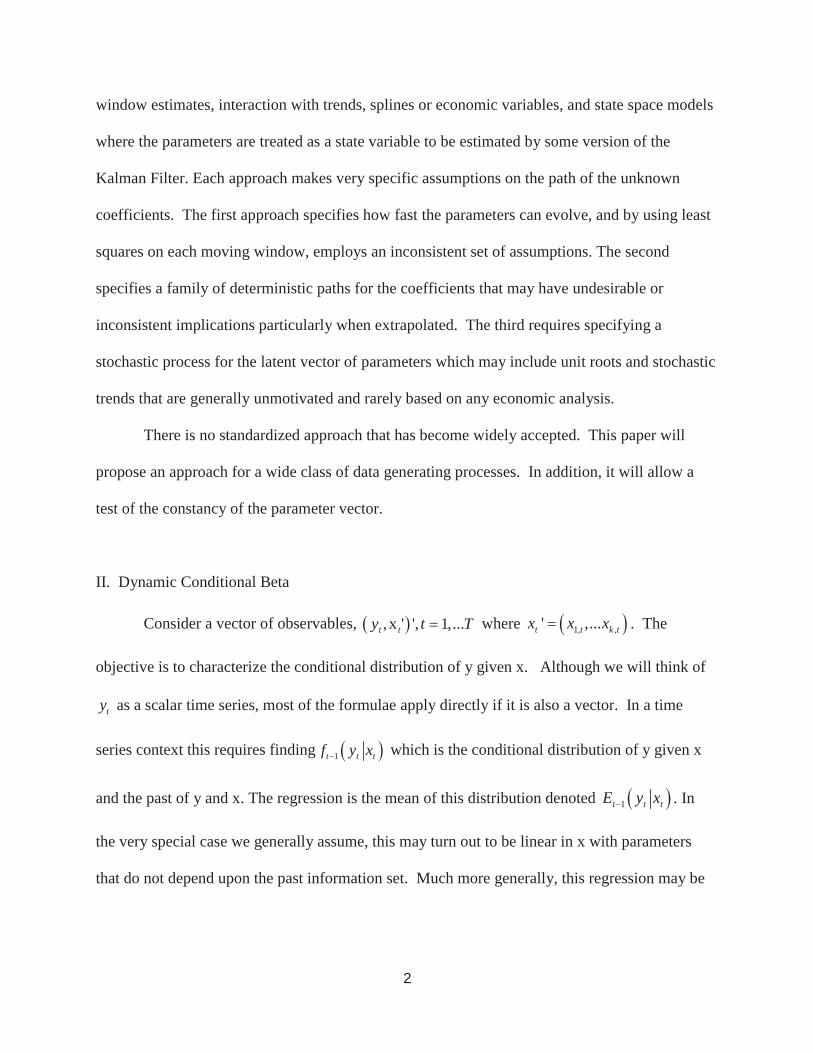
DYNAMIC CONDITIONAL BETA
Robert Engle1
February 27, 2014
ABSTRACT
Dynamic Conditional Beta (DCB) is an approach to estimating regressions with time varying parameters. The conditional covariance matrices of the exogenous and dependent variable for each time period are used to formulate the dynamic beta. Joint estimation of the covariance matrices and other regression parameters is developed. Tests of the hypothesis that betas are constant are non-nested tests and several approaches are developed including a novel nested model. The methodology is applied to industry multifactor asset pricing and to global systemic risk estimation with non-synchronous prices.
Keywords: GARCH, DCC, Time Varying Parameters, Multivariate GARCH, Non-Nested Tests, Multi-factor Asset Pricing, Systemic Risk, SRISK
I. Introduction
In empirical finance and in time series applied economics in general, the least squares
model is the workhorse. In class there is much discussion of the assumptions of exogeneity,
homoskedasticity and serial correlation. However in practice it may be unstable regression
coefficients that are most troubling. Rarely is there a credible economic rationale for the
assumption that the slope coefficients are time invariant.
Econometricians have developed a variety of statistical methodologies for dealing with
time series regression models with time varying parameters. The three most common are rolling
1 Robert Engle is Director of the Volatility Institute of NYU’s Stern School of Business and Professor of Finance. He appreciates comments and suggestions from many people on this paper, particularly participants at Oxford’s Launch of EMoD, SoFiE Singapore, and the University of Chicago Booth Seminar. Particular thanks go to Viral Acharya, Turan Bali, Niel Ericsson, Gene Fama, Eric Ghysels, Jim Hamilton, David Hendry, Alain Monfort, Matt Richardson, Jeff Wooldridge and to Rob Capellini, Hahn Le, and Emil Siriwadane.
1
window estimates, interaction with trends, splines or economic variables, and state space models
where the parameters are treated as a state variable to be estimated by some version of the
Kalman Filter. Each approach makes very specific assumptions on the path of the unknown
coefficients. The first approach specifies how fast the parameters can evolve, and by using least
squares on each moving window, employs an inconsistent set of assumptions. The second
specifies a family of deterministic paths for the coefficients that may have undesirable or
inconsistent implications particularly when extrapolated. The third requires specifying a
stochastic process for the latent vector of parameters which may include unit roots and stochastic
trends that are generally unmotivated and rarely based on any economic analysis.
There is no standardized approach that has become widely accepted. This paper will
propose an approach for a wide class of data generating processes. In addition, it will allow a
test of the constancy of the parameter vector.
II. Dynamic Conditional Beta
Consider a vector of observables, , x ' ', 1,...t ty t T where 1, ,' ,...t t k tx x x . The
objective is to characterize the conditional distribution of y given x. Although we will think of
ty as a scalar time series, most of the formulae apply directly if it is also a vector. In a time
series context this requires finding 1t t tf y x which is the conditional distribution of y given x
and the past of y and x. The regression is the mean of this distribution denoted 1t t tE y x . In
the very special case we generally assume, this may turn out to be linear in x with parameters
that do not depend upon the past information set. Much more generally, this regression may be
2
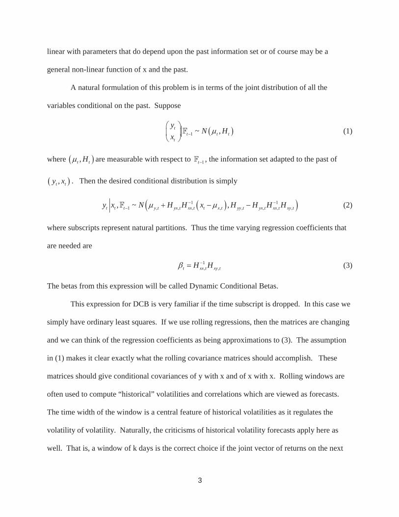
linear with parameters that do depend upon the past information set or of course may be a
general non-linear function of x and the past.
A natural formulation of this problem is in terms of the joint distribution of all the
variables conditional on the past. Suppose
1 ~ ,tt t t
t
yN H
x(1)
where ,t tH are measurable with respect to 1t , the information set adapted to the past of
,t ty x . Then the desired conditional distribution is simply
1 11 , , , , , , , ,, ~ ,t t t y t yx t xx t t x t yy t yx t xx t xy ty x N H H x H H H H (2)
where subscripts represent natural partitions. Thus the time varying regression coefficients that
are needed are
1, ,t xx t xy tH H (3)
The betas from this expression will be called Dynamic Conditional Betas.
This expression for DCB is very familiar if the time subscript is dropped. In this case we
simply have ordinary least squares. If we use rolling regressions, then the matrices are changing
and we can think of the regression coefficients as being approximations to (3). The assumption
in (1) makes it clear exactly what the rolling covariance matrices should accomplish. These
matrices should give conditional covariances of y with x and of x with x. Rolling windows are
often used to compute “historical” volatilities and correlations which are viewed as forecasts.
The time width of the window is a central feature of historical volatilities as it regulates the
volatility of volatility. Naturally, the criticisms of historical volatility forecasts apply here as
well. That is, a window of k days is the correct choice if the joint vector of returns on the next
3
day is equally likely to come from any of the previous k days but could not be from returns more
than k days in the past. Because of the unrealistic nature of this specification, exponential
smoothing is a better alternative for most cases.
The normality assumption is obviously restrictive but can be generalized. For example,
if the joint distribution in (1) is in the elliptical family of distributions, then (2) holds with the
appropriate elliptical distribution. Even without elliptical distributions, (2) can be interpreted as
the conditional linear projection. The projection may be linear but with a non-normal error
which will support estimation as in Brownlees and Engle(2011). The more difficult issue is that
we do not observe directly either the vector of conditional means or conditional covariances. A
model is required for each of these. For many financial applications where the data are returns,
the mean is relatively unimportant and attention can be focused on the conditional covariance
matrix. Think for a moment of the estimate of the beta of a stock or portfolio, or multiple betas
in factor models, style models of portfolios, or the pricing kernel, and many other examples. In
these cases, a natural approach is to use a general covariance matrix estimator and then calculate
the betas.
It is important to recognize that equation (3) is a natural extension of estimators that have
long been used in time series. Probably the first application was Bollerslev, Engle and
Wooldridge(1988) where the beta was computed as the ratio of the conditional covariance to the
conditional variance. One of the leading applications of multivariate GARCH models has
always been estimation of hedge ratios. This is discussed in surveys such as Bollerslev, Chou
and Kroner(1994), Bollerslev, Engle and Nelson(2004), Bera and Higgins(1993) and Lien and
Tse(2002). Specific hedging models are proposed by Kroner and Sultan(1993), Cecchetti,
Cumby and Figlewski(1998), Bera, Garcia and Roh(1997) and Braun, Nelson and Sunier(1995).
4
More recently, hedging performance is used as a test of the multivariate garch specification in
Engle(9), and Lien, Tse and Tsui(2002) among others. Recent applications to asset pricing and
systemic risk are in Bali, Engle and Tang(2012) and Brownlees and Engle(2012). When data are
available at a higher frequency than the analysis, estimates of realized variances, realized
covariances and realized betas can be constructed. These realized betas are time varying and can
be directly forecast and modeled. See for example Andersen, Bollerslev, Diebold and
Wu(2005)(2006) and Patten and Verardo(2012).
All of these examples would be considered as Dynamic Conditional Betas by the
description above. Almost all of these applications involve only bivariate models where there is
just one covariance to be estimated and the hedge ratio is simply the ratio of the conditional
covariance to the conditional variance. In no case is there a statistical test of the null hypothesis
that the beta is truly constant. There is no discussion of maximum likelihood estimation in these
more general contexts.
This paper will extend the analysis of dynamic conditional betas into a multivariate
context and then explicitly consider the estimation and testing of the model from a classical
perspective. The tools developed here would have been useful for many of these prior studies.
III. Maximum Likelihood Estimation of DCB
A. All betas are varying
Maximum likelihood estimation of the Dynamic Conditional Beta model requires
specification of both the covariance matrix and the mean of the data vector. In general, the
covariance matrix and mean of these data will include unknown parameters. Extending equation
(1) to include a jx1 vector of unknown parameters in the mean and variance equations, we get
5
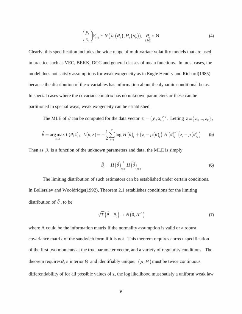
1 0 0 01
~ , ,tt t t
jxt
yN H
x (4)
Clearly, this specification includes the wide range of multivariate volatility models that are used
in practice such as VEC, BEKK, DCC and general classes of mean functions. In most cases, the
model does not satisfy assumptions for weak exogeneity as in Engle Hendry and Richard(1985)
because the distribution of the x variables has information about the dynamic conditional betas.
In special cases where the covariance matrix has no unknown parameters or these can be
partitioned in special ways, weak exogeneity can be established.
The MLE of can be computed for the data vector , ' 't t tz y x . Letting 1,..., Tz z z ,
1
1
1ˆ arg max ; , ; log '2
T
t tt t t tt
L z L z H z H z (5)
Then as t is a function of the unknown parameters and data, the MLE is simply
1
, ,ˆ ˆ ˆ
t xx t xy tH H (6)
The limiting distribution of such estimators can be established under certain conditions.
In Bollerslev and Wooldridge(1992), Theorem 2.1 establishes conditions for the limiting
distribution of ˆ , to be
10
ˆ 0,T N A (7)
where A could be the information matrix if the normality assumption is valid or a robust
covariance matrix of the sandwich form if it is not. This theorem requires correct specification
of the first two moments at the true parameter vector, and a variety of regularity conditions. The
theorem requires 0 interior and identifiably unique. , H must be twice continuous
differentiability of for all possible values of z, the log likelihood must satisfy a uniform weak law
6
of large numbers, the score vector must satisfy a central limit theorem and the Hessian must
satisfy a law of large numbers and converge to a non-singular matrix. Some of these conditions
can be weakened , particularly in the context of stationary ergodic random variables.
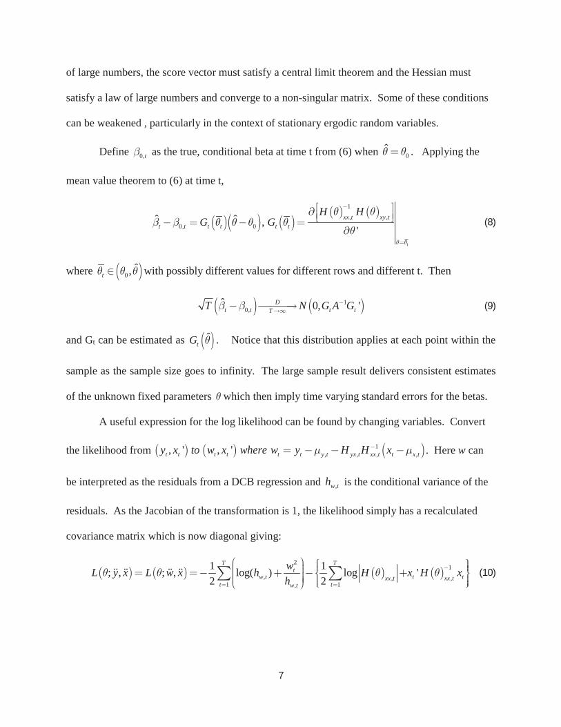
Define 0,t as the true, conditional beta at time t from (6) when 0ˆ . Applying the
mean value theorem to (6) at time t,
1
, ,0, 0
ˆ ˆ ,'
t
xx t xy tt t t t t t
H HG G (8)
where 0ˆ,t with possibly different values for different rows and different t. Then
10,
ˆ 0, 'Dt t t tTT N G A G (9)
and Gt can be estimated as ˆtG . Notice that this distribution applies at each point within the
sample as the sample size goes to infinity. The large sample result delivers consistent estimates
of the unknown fixed parameters which then imply time varying standard errors for the betas.
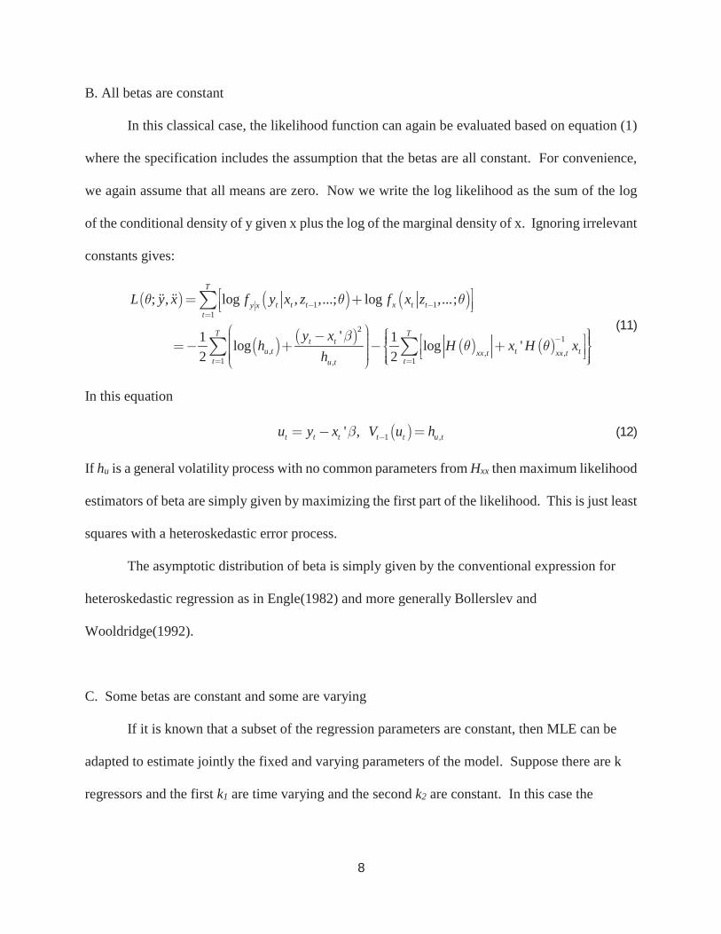
A useful expression for the log likelihood can be found by changing variables. Convert
the likelihood from 1, , , ,, ' , 't t t t t t y t yx t xx t t x ty x to w x where w y H H x . Here w can
be interpreted as the residuals from a DCB regression and ,w th is the conditional variance of the
residuals. As the Jacobian of the transformation is 1, the likelihood simply has a recalculated
covariance matrix which is now diagonal giving:
21
, , ,1 1,
1 1; , ; , log( ) log '2 2
T Tt
w t t txx t xx tt tw t
wL y x L w x h H x H xh
(10)
7
B. All betas are constant
In this classical case, the likelihood function can again be evaluated based on equation (1)
where the specification includes the assumption that the betas are all constant. For convenience,
we again assume that all means are zero. Now we write the log likelihood as the sum of the log
of the conditional density of y given x plus the log of the marginal density of x. Ignoring irrelevant
constants gives:
1 11
21
, , ,1 1,
; , log , ,...; log ,...;
'1 1log log '2 2
T
t t t x t ty xt
T Tt t
u t t txx t xx tt tu t
L y x f y x z f x z
y xh H x H x
h
(11)
In this equation
1 ,' ,t t t t t u tu y x V u h (12)
If hu is a general volatility process with no common parameters from Hxx then maximum likelihood
estimators of beta are simply given by maximizing the first part of the likelihood. This is just least
squares with a heteroskedastic error process.
The asymptotic distribution of beta is simply given by the conventional expression for
heteroskedastic regression as in Engle(1982) and more generally Bollerslev and
Wooldridge(1992).
C. Some betas are constant and some are varying
If it is known that a subset of the regression parameters are constant, then MLE can be
adapted to estimate jointly the fixed and varying parameters of the model. Suppose there are k
regressors and the first k1 are time varying and the second k2 are constant. In this case the
8
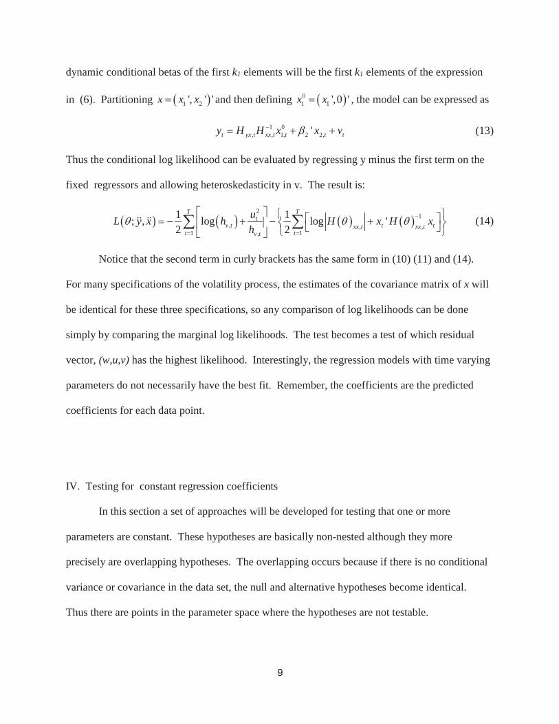
dynamic conditional betas of the first k1 elements will be the first k1 elements of the expression
in (6). Partitioning 1 2', ' 'x x x and then defining 01 1 ',0 'x x , the model can be expressed as
1 0, , 1, 2 2,'t yx t xx t t t ty H H x x v (13)
Thus the conditional log likelihood can be evaluated by regressing y minus the first term on the
fixed regressors and allowing heteroskedasticity in v. The result is:
21
, , ,1 1,
1 1; , log log '2 2
T Tt
v t t txx t xx tt tv t
uL y x h H x H xh
(14)
Notice that the second term in curly brackets has the same form in (10) (11) and (14).
For many specifications of the volatility process, the estimates of the covariance matrix of x will
be identical for these three specifications, so any comparison of log likelihoods can be done
simply by comparing the marginal log likelihoods. The test becomes a test of which residual
vector, (w,u,v) has the highest likelihood. Interestingly, the regression models with time varying
parameters do not necessarily have the best fit. Remember, the coefficients are the predicted
coefficients for each data point.
IV. Testing for constant regression coefficients
In this section a set of approaches will be developed for testing that one or more
parameters are constant. These hypotheses are basically non-nested although they more
precisely are overlapping hypotheses. The overlapping occurs because if there is no conditional
variance or covariance in the data set, the null and alternative hypotheses become identical.
Thus there are points in the parameter space where the hypotheses are not testable.
9
There are several standard approaches to testing non-nested hypotheses. The first
developed initially by Cox(1961,1962) is a model selection approach which simply asks which
model has the highest value of a (possibly penalized) likelihood. If there are two models being
considered, there are two possible outcomes.
A second approach introduced by Vuong(1989) is to form a two tailed test of the
hypothesis that the models are equally close to the true model. In this case, there are three
possible outcomes, model 1, model 2, and that models are equivalent.
A third approach is artificial nesting as discussed in Cox(1961,1962) and advocated by
Aitkinson(1970) An artificial model is constructed that nests both special cases. When this
strategy is used to compare two models, there are generally four possible outcomes – model 1,
model 2, both , neither. Artifical nesting of hypotheses is a powerful approach in this context as
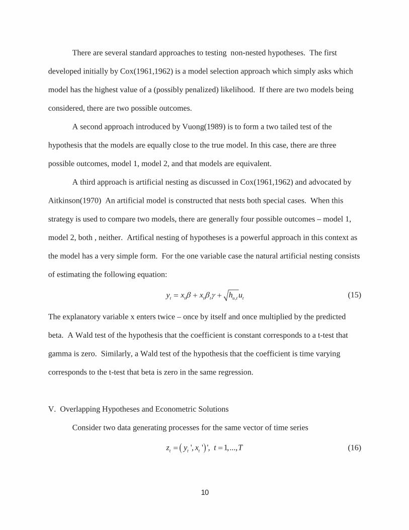
the model has a very simple form. For the one variable case the natural artificial nesting consists
of estimating the following equation:
,t t t t u t ty x x h u (15)
The explanatory variable x enters twice – once by itself and once multiplied by the predicted
beta. A Wald test of the hypothesis that the coefficient is constant corresponds to a t-test that
gamma is zero. Similarly, a Wald test of the hypothesis that the coefficient is time varying
corresponds to the t-test that beta is zero in the same regression.
V. Overlapping Hypotheses and Econometric Solutions
Consider two data generating processes for the same vector of time series
', ' ', 1,...,t t tz y x t T (16)
10
In the simplest case, there is only one endogenous variable and k conditioning variables. These
can be expressed in terms of the joint distributions conditional on past information as:
1
1
~ , ,
~ , ,t t t t
t t t t
z f z
z g z(17)
Without loss of generality we can write each distribution conditional on the past as the product of
a conditional and a marginal distribution each conditioned on the past.
,,
,,
; ; ;
; ; ;
t t t t x t ty x t
t t t t x t ty x t
f z f y x f x
g z g y x g x (18)
The maximized log likelihoods of these models are given by
,,1
,,1
ˆ ˆ ˆlog ; log ;
ˆ ˆ ˆlog ; log ;
T
f t t x t ty x ttT
g t t x t ty x tt
L f y x f x
L g y x g x (19)
Model f is said to be nested within g if for every 0 there is a * such that
, , *of z g z so that events have the same probability whether , of z or , *g z is
the true DGP. A similar definition applies to the notion that g is nested within f. The models f
and g are partially non-nested (Cox(1960),1961), Pesaran(1999)) or overlapping (Vuong(1989))
if there are some parameters in that lead to identical distributions. Vuong proposes a
sequential procedure that tests for such parameters first and upon rejecting these cases, examines
the purely non-nested case. The parameters and include parameters of the covariance
matrix that must be estimated as well as parameters of the regression function such as the betas.
The parameters of the covariance matrix could be the parameters of a multivariate GARCH
model if that is how the estimation is conducted. If a DCC approach is used, then the parameters
11
would include both GARCH parameters and DCC parameters. From equation (3) and
knowledge of a wide range of multivariate GARCH models, it is apparent that the only point in
the parameter space where the fixed parameter and varying parameter are equivalent is the point
where there is no conditional heteroskedasticity in the observables. Even models like constant
conditional correlation, BEKK, VEC and DECO have no parameters that will make the betas in
(3) constant unless both ,xx tH and ,xy tH are themselves constant. Thus it is essential to
determine whether there is heteroskedasticity in y and x to ensure that this is a non-nested
problem.
As discussed above, several approaches to model building for non-nested models will be
applied.
a) Model Selection
From the maximized likelihood in (19) and a penalty function such as Schwarz or
Aikaike, the selected model can be directly found. The criterion function is the penalized
likelihood ratio given by
, ,1 1
ˆ ˆlog ; log ;T T
T z t t z t t f gt t
LR f z g z pen pen (20)
A positive value of LR selects f and a negative value selects g. For the Aikaike Information
Criterion (AIC), f g f gpen pen k k and for the Schwarz or Bayesian Information
Criterion, (BIC) it is given by *log / 2f gk k T Here k is the total number of estimated
parameters in each model. Clearly, as T becomes large, the penalty becomes irrelevant in model
selection.
In many cases the likelihood will have the same estimate of the likelihood of the
conditioning variables, x, and consequently the maximized values will satisfy
12
, ,1 1
ˆ ˆlog ; log ;T T
x t t x t tt t
f x g x (21)
This will happen if the dynamic covariance matrix of the x variables is estimated the same way
regardless of the specification of the dynamics of the regression coefficients. Therefore model
selection will only involve the first term in the log likelihood just as in a conventional regression.
Thus model selection can be based on
, ,1 1
ˆ ˆlog ; log ;T T
T t t t t f gy x t y x tt t
LR f y x g y x pen pen (22)
which can be expressed in terms of the residuals as in equations (10), (11) and (14). Model
selection between DCB and constant betas can be based on the penalized log likelihood
2 2
, ,1 1, ,
log logT T
t tT w t u t w u
t tw t u t
w uLR h h pen penh h
(23)
The penalties will depend upon the number of parameters estimated in each model. Since the
parameters in the x matrix are the same and the parameters in the error process are the same, the
only difference is the number of fixed betas that are estimated.
b) Testing Model Equality.
Following Vuong(1989) and Rivers and Vuong(2002), the model selection procedure can
be given a testing framework. The criterion in (22) has a distribution under the null hypothesis
that the two likelihoods are the same. The hypothesis that the likelihoods are the same is
interpreted by Vuong as the hypothesis that they are equally close in a Kulbach Leibler sense, to
the true DGP. He shows that under this null, the LR criterion converges to a Gaussian
distribution with a variance that can be estimated simply from the maximized likelihood ratio
statistic. Letting
13
,
,
ˆ;log
ˆ;t ty x t
tt ty x t
f y xm
g y x(24)
then
22
1
1ˆ /T
t Tt
m LR TT
(25)
and it is shown in Theorem 5.1 that
1/2 ˆ/ 0,1dTT LR N (26)
This can be computed as the t-statistic on the intercept in a regression of mt on a constant. Based
on this limiting argument, three critical regions can be established – select model f, select model
g, they are equivalent.
To apply this approach we substitute the log likelihood of the DCB model and the fixed
coefficient GARCH model into (24). From (11) and (14) we get
2 2, , , , , ,.5 log /t f t g t f t g t f t g tm L L h h (27)
If a finite sample penalty for the number of parameters is adapted such as the Schwarz criterion,
then the definition of m becomes
2 2, , , ,.5 log / log /t f t g t f t g t f gm h h k k T T (28)
This series of penalized log differences is regressed on a constant and the robust t-statistic is
reported. If it is significantly positive, then model f is preferred and if significantly negative,
then model g is preferred. As m in equation (28) is likely to have autocorrelation, the t-statistic
should be computed with a HAC standard error that is robust to autocorrelation and
heteroskedasticity. See Rivers and Vuong(2002).
c) The third approach is based on artificial nesting and, as discussed above in (15), is
simply an augmented regression model which allows for heteroskedasticity. From asymptotic
14
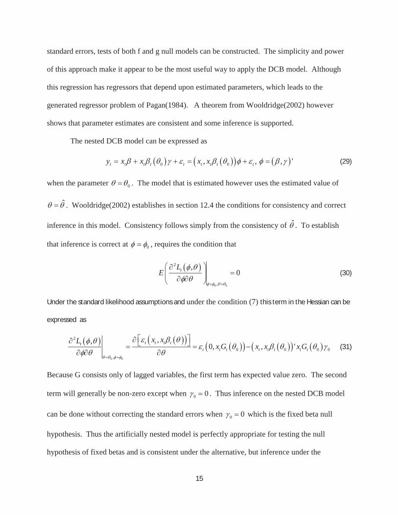
standard errors, tests of both f and g null models can be constructed. The simplicity and power
of this approach make it appear to be the most useful way to apply the DCB model. Although
this regression has regressors that depend upon estimated parameters, which leads to the
generated regressor problem of Pagan(1984). A theorem from Wooldridge(2002) however
shows that parameter estimates are consistent and some inference is supported.
The nested DCB model can be expressed as
0 0, , , 't t t t t t t t ty x x x x (29)
when the parameter 0 . The model that is estimated however uses the estimated value of
ˆ . Wooldridge(2002) establishes in section 12.4 the conditions for consistency and correct
inference in this model. Consistency follows simply from the consistency of ˆ . To establish
that inference is correct at 0 , requires the condition that
0 0
2
,
,0tL
E (30)
Under the standard likelihood assumptions and under the condition (7) this term in the Hessian can be
expressed as
0 0
2
0 0 0 0
,
,,0, , 't t t tt
t t t t t t t t
x xLx G x x x G (31)
Because G consists only of lagged variables, the first term has expected value zero. The second
term will generally be non-zero except when 0 0 . Thus inference on the nested DCB model
can be done without correcting the standard errors when 0 0 which is the fixed beta null
hypothesis. Thus the artificially nested model is perfectly appropriate for testing the null
hypothesis of fixed betas and is consistent under the alternative, but inference under the
15
alternative should be adjusted. An approach to this inference problem can be developed
following Wooldridge but this has not yet been worked out.
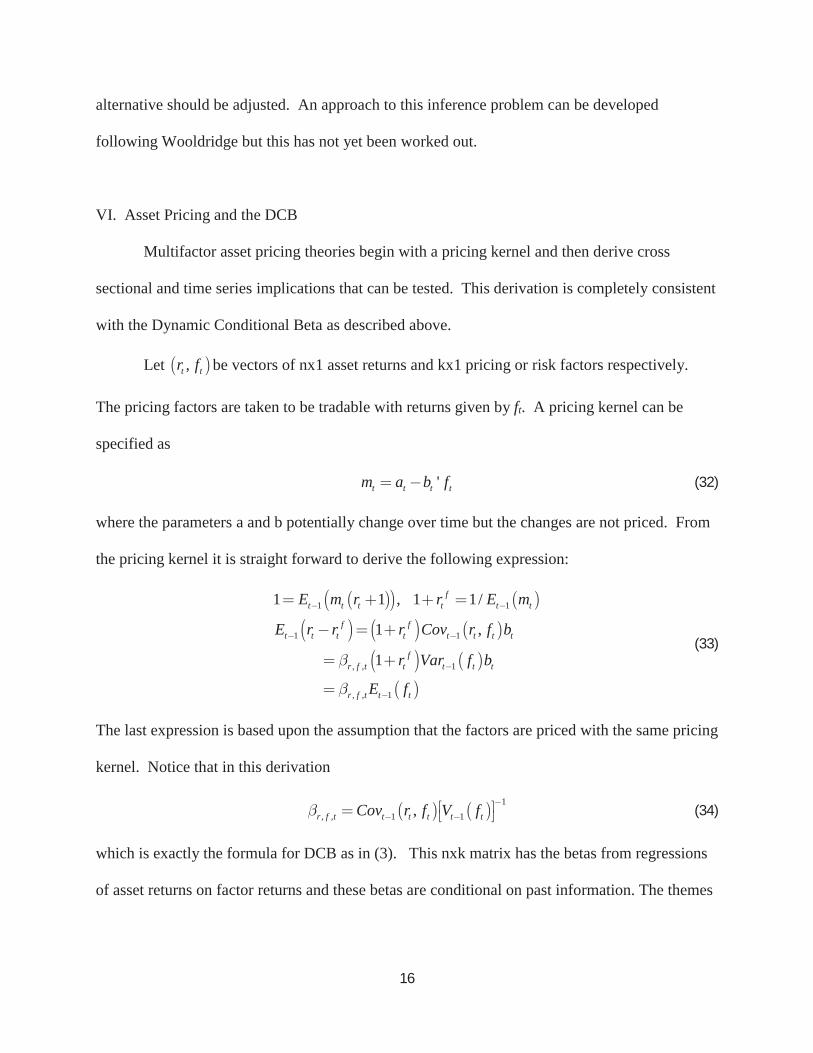
VI. Asset Pricing and the DCB
Multifactor asset pricing theories begin with a pricing kernel and then derive cross
sectional and time series implications that can be tested. This derivation is completely consistent
with the Dynamic Conditional Beta as described above.
Let ,t tr f be vectors of nx1 asset returns and kx1 pricing or risk factors respectively.
The pricing factors are taken to be tradable with returns given by ft. A pricing kernel can be
specified as
't t t tm a b f (32)
where the parameters a and b potentially change over time but the changes are not priced. From
the pricing kernel it is straight forward to derive the following expression:
1 1
1 1
, , 1
, , 1
1 1 , 1 1/
1 ,
1
ft t t t t t
f ft t t t t t t t
fr f t t t t t
r f t t t
E m r r E m
E r r r Cov r f b
r Var f b
E f
(33)
The last expression is based upon the assumption that the factors are priced with the same pricing
kernel. Notice that in this derivation
1, , 1 1,r f t t t t t tCov r f V f (34)
which is exactly the formula for DCB as in (3). This nxk matrix has the betas from regressions
of asset returns on factor returns and these betas are conditional on past information. The themes
16
of asset pricing come through completely in that the expected return on an asset is linear in beta
and depends upon the risk premium embedded in the factor.
In Bali, Engle and Tang(2012) this empirical model is challenged to explain cross
sectional returns in a one factor dynamic model. It performs very well providing new evidence
of the power of beta when it is estimated dynamically. Furthermore, they find strong evidence of
hedging demand in the conditional ICAPM. In Bali and Engle(2010) a similar model is
examined from a pooled time series cross section point of view and again evidence is found for
hedging demands. It is found that the most useful second factor is a volatility factor.
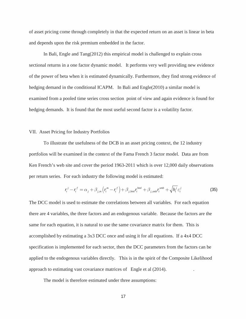
VII. Asset Pricing for Industry Portfolios
To illustrate the usefulness of the DCB in an asset pricing context, the 12 industry
portfolios will be examined in the context of the Fama French 3 factor model. Data are from
Ken French’s web site and cover the period 1963-2011 which is over 12,000 daily observations
per return series. For each industry the following model is estimated:
, , ,j f m f hml smb j j
t t j j m t t j hml t j smb t t tr r r r r r h (35)
The DCC model is used to estimate the correlations between all variables. For each equation
there are 4 variables, the three factors and an endogenous variable. Because the factors are the
same for each equation, it is natural to use the same covariance matrix for them. This is
accomplished by estimating a 3x3 DCC once and using it for all equations. If a 4x4 DCC
specification is implemented for each sector, then the DCC parameters from the factors can be
applied to the endogenous variables directly. This is in the spirit of the Composite Likelihood
approach to estimating vast covariance matrices of Engle et al (2014). .
The model is therefore estimated under three assumptions:
17
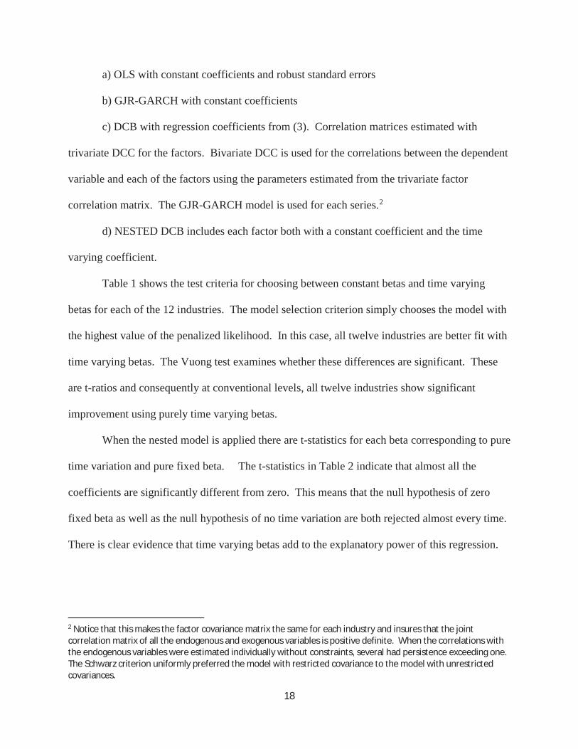
a) OLS with constant coefficients and robust standard errors
b) GJR-GARCH with constant coefficients
c) DCB with regression coefficients from (3). Correlation matrices estimated with
trivariate DCC for the factors. Bivariate DCC is used for the correlations between the dependent
variable and each of the factors using the parameters estimated from the trivariate factor
correlation matrix. The GJR-GARCH model is used for each series.2
d) NESTED DCB includes each factor both with a constant coefficient and the time
varying coefficient.
Table 1 shows the test criteria for choosing between constant betas and time varying
betas for each of the 12 industries. The model selection criterion simply chooses the model with
the highest value of the penalized likelihood. In this case, all twelve industries are better fit with
time varying betas. The Vuong test examines whether these differences are significant. These
are t-ratios and consequently at conventional levels, all twelve industries show significant
improvement using purely time varying betas.
When the nested model is applied there are t-statistics for each beta corresponding to pure
time variation and pure fixed beta. The t-statistics in Table 2 indicate that almost all the
coefficients are significantly different from zero. This means that the null hypothesis of zero
fixed beta as well as the null hypothesis of no time variation are both rejected almost every time.
There is clear evidence that time varying betas add to the explanatory power of this regression.
2 Notice that this makes the factor covariance matrix the same for each industry and insures that the joint correlation matrix of all the endogenous and exogenous variables is positive definite. When the correlations with the endogenous variables were estimated individually without constraints, several had persistence exceeding one. The Schwarz criterion uniformly preferred the model with restricted covariance to the model with unrestricted covariances.
18
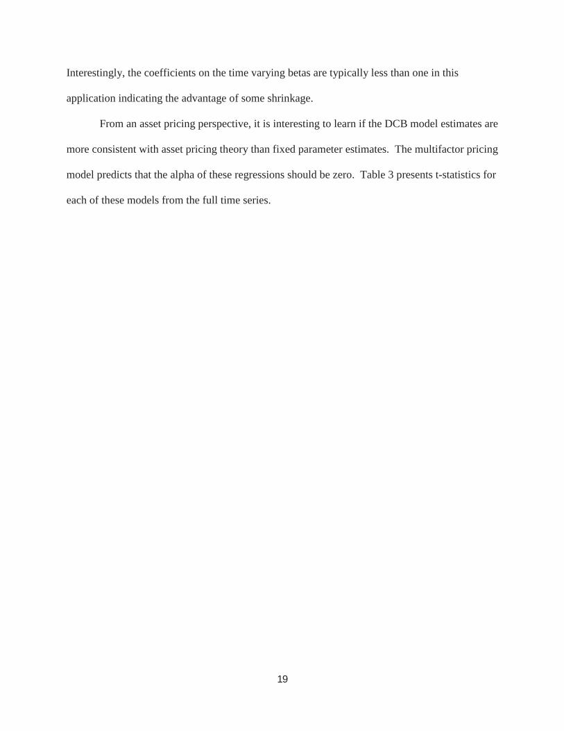
Interestingly, the coefficients on the time varying betas are typically less than one in this
application indicating the advantage of some shrinkage.
From an asset pricing perspective, it is interesting to learn if the DCB model estimates are
more consistent with asset pricing theory than fixed parameter estimates. The multifactor pricing
model predicts that the alpha of these regressions should be zero. Table 3 presents t-statistics for
each of these models from the full time series.
19
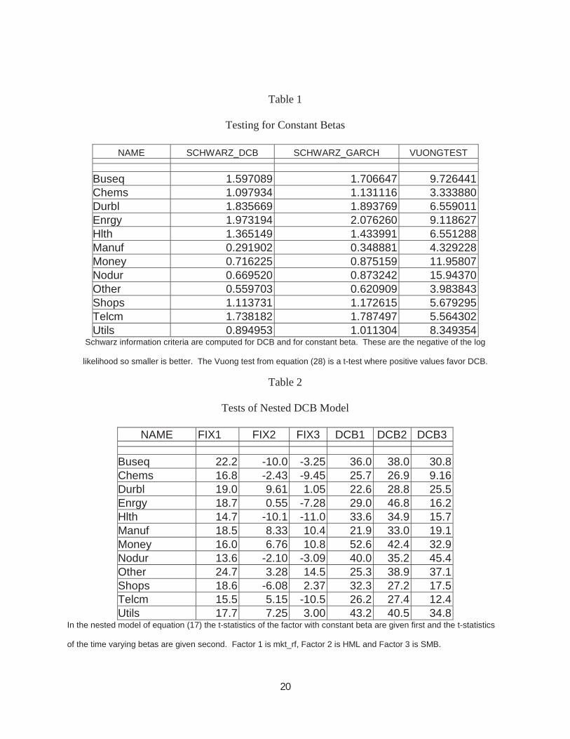
Table 1
Testing for Constant Betas
NAME SCHWARZ_DCB SCHWARZ_GARCH VUONGTEST
Buseq 1.597089 1.706647 9.726441Chems 1.097934 1.131116 3.333880Durbl 1.835669 1.893769 6.559011Enrgy 1.973194 2.076260 9.118627Hlth 1.365149 1.433991 6.551288Manuf 0.291902 0.348881 4.329228Money 0.716225 0.875159 11.95807Nodur 0.669520 0.873242 15.94370Other 0.559703 0.620909 3.983843Shops 1.113731 1.172615 5.679295Telcm 1.738182 1.787497 5.564302Utils 0.894953 1.011304 8.349354
Schwarz information criteria are computed for DCB and for constant beta. These are the negative of the log
likelihood so smaller is better. The Vuong test from equation (28) is a t-test where positive values favor DCB.
Table 2
Tests of Nested DCB Model
NAME FIX1 FIX2 FIX3 DCB1 DCB2 DCB3
Buseq 22.2 -10.0 -3.25 36.0 38.0 30.8Chems 16.8 -2.43 -9.45 25.7 26.9 9.16Durbl 19.0 9.61 1.05 22.6 28.8 25.5Enrgy 18.7 0.55 -7.28 29.0 46.8 16.2Hlth 14.7 -10.1 -11.0 33.6 34.9 15.7Manuf 18.5 8.33 10.4 21.9 33.0 19.1Money 16.0 6.76 10.8 52.6 42.4 32.9Nodur 13.6 -2.10 -3.09 40.0 35.2 45.4Other 24.7 3.28 14.5 25.3 38.9 37.1Shops 18.6 -6.08 2.37 32.3 27.2 17.5Telcm 15.5 5.15 -10.5 26.2 27.4 12.4Utils 17.7 7.25 3.00 43.2 40.5 34.8
In the nested model of equation (17) the t-statistics of the factor with constant beta are given first and the t-statistics
of the time varying betas are given second. Factor 1 is mkt_rf, Factor 2 is HML and Factor 3 is SMB.
20
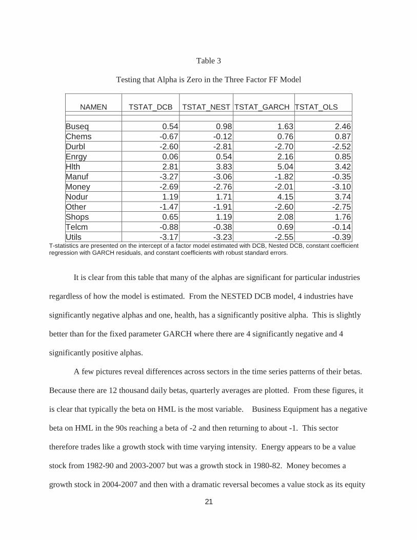
Table 3
Testing that Alpha is Zero in the Three Factor FF Model
NAMEN TSTAT_DCB TSTAT_NEST
TSTAT_GARCH TSTAT_OLS
Buseq 0.54 0.98 1.63 2.46Chems -0.67 -0.12 0.76 0.87Durbl -2.60 -2.81 -2.70 -2.52Enrgy 0.06 0.54 2.16 0.85Hlth 2.81 3.83 5.04 3.42Manuf -3.27 -3.06 -1.82 -0.35Money -2.69 -2.76 -2.01 -3.10Nodur 1.19 1.71 4.15 3.74Other -1.47 -1.91 -2.60 -2.75Shops 0.65 1.19 2.08 1.76Telcm -0.88 -0.38 0.69 -0.14Utils -3.17 -3.23 -2.55 -0.39
T-statistics are presented on the intercept of a factor model estimated with DCB, Nested DCB, constant coefficient regression with GARCH residuals, and constant coefficients with robust standard errors.
It is clear from this table that many of the alphas are significant for particular industries
regardless of how the model is estimated. From the NESTED DCB model, 4 industries have
significantly negative alphas and one, health, has a significantly positive alpha. This is slightly
better than for the fixed parameter GARCH where there are 4 significantly negative and 4
significantly positive alphas.
A few pictures reveal differences across sectors in the time series patterns of their betas.
Because there are 12 thousand daily betas, quarterly averages are plotted. From these figures, it
is clear that typically the beta on HML is the most variable. Business Equipment has a negative
beta on HML in the 90s reaching a beta of -2 and then returning to about -1. This sector
therefore trades like a growth stock with time varying intensity. Energy appears to be a value
stock from 1982-90 and 2003-2007 but was a growth stock in 1980-82. Money becomes a
growth stock in 2004-2007 and then with a dramatic reversal becomes a value stock as its equity
21
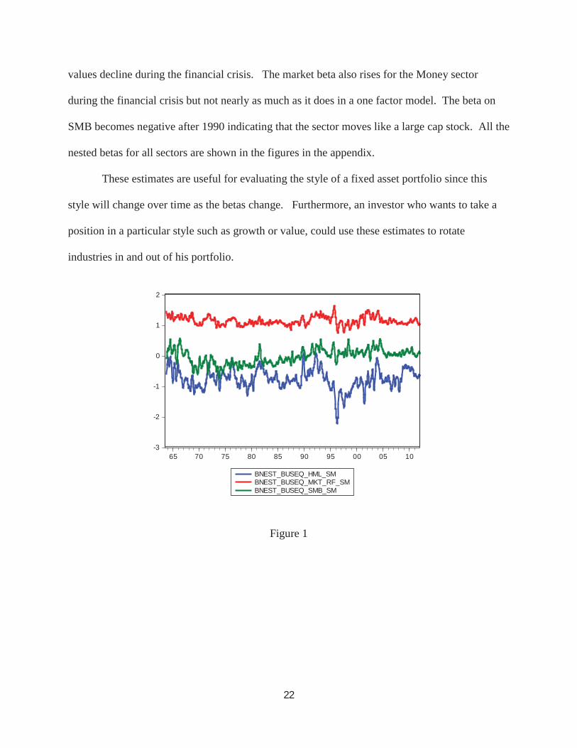
values decline during the financial crisis. The market beta also rises for the Money sector
during the financial crisis but not nearly as much as it does in a one factor model. The beta on
SMB becomes negative after 1990 indicating that the sector moves like a large cap stock. All the
nested betas for all sectors are shown in the figures in the appendix.
These estimates are useful for evaluating the style of a fixed asset portfolio since this
style will change over time as the betas change. Furthermore, an investor who wants to take a
position in a particular style such as growth or value, could use these estimates to rotate
industries in and out of his portfolio.
Figure 1
-3
-2
-1
0
1
2
65 70 75 80 85 90 95 00 05 10
BNEST_BUSEQ_HML_SMBNEST_BUSEQ_MKT_RF_SMBNEST_BUSEQ_SMB_SM
22
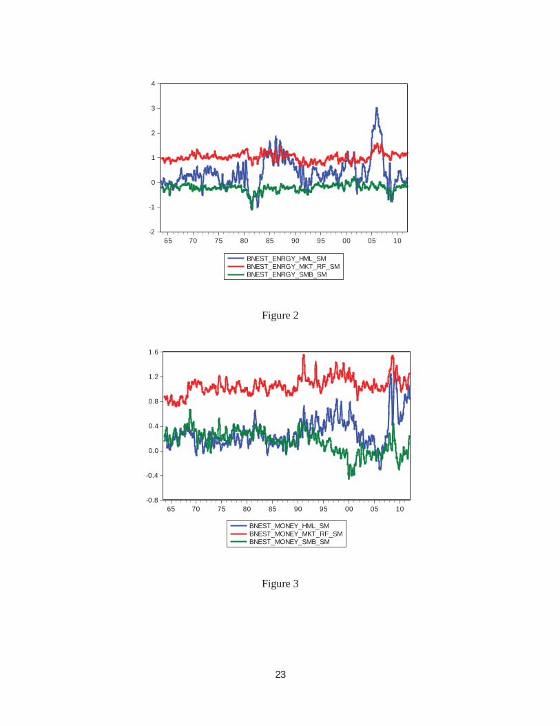
Figure 2
Figure 3
-2
-1
0
1
2
3
4
65 70 75 80 85 90 95 00 05 10
BNEST_ENRGY_HML_SMBNEST_ENRGY_MKT_RF_SMBNEST_ENRGY_SMB_SM
-0.8
-0.4
0.0
0.4
0.8
1.2
1.6
65 70 75 80 85 90 95 00 05 10
BNEST_MONEY_HML_SMBNEST_MONEY_MKT_RF_SMBNEST_MONEY_SMB_SM
23
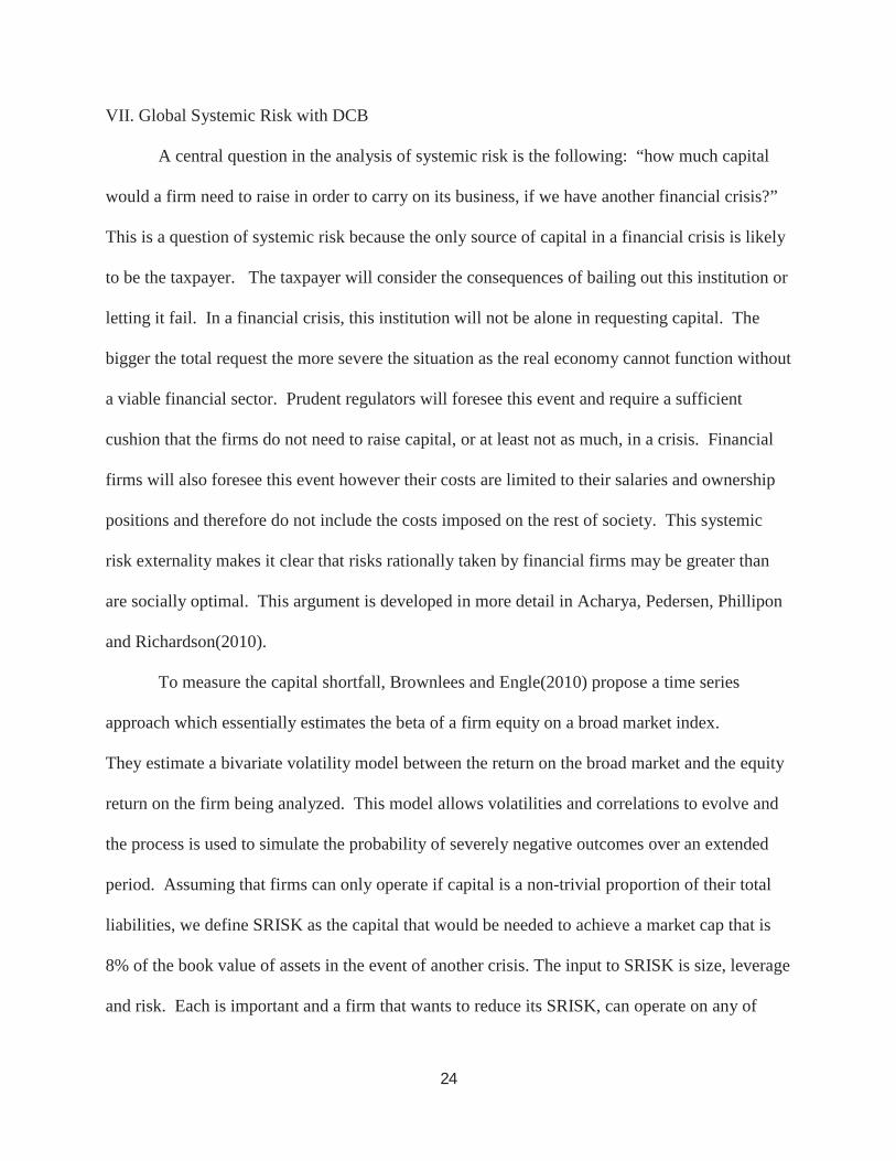
VII. Global Systemic Risk with DCB
A central question in the analysis of systemic risk is the following: “how much capital
would a firm need to raise in order to carry on its business, if we have another financial crisis?”
This is a question of systemic risk because the only source of capital in a financial crisis is likely
to be the taxpayer. The taxpayer will consider the consequences of bailing out this institution or
letting it fail. In a financial crisis, this institution will not be alone in requesting capital. The
bigger the total request the more severe the situation as the real economy cannot function without
a viable financial sector. Prudent regulators will foresee this event and require a sufficient
cushion that the firms do not need to raise capital, or at least not as much, in a crisis. Financial
firms will also foresee this event however their costs are limited to their salaries and ownership
positions and therefore do not include the costs imposed on the rest of society. This systemic
risk externality makes it clear that risks rationally taken by financial firms may be greater than
are socially optimal. This argument is developed in more detail in Acharya, Pedersen, Phillipon
and Richardson(2010).
To measure the capital shortfall, Brownlees and Engle(2010) propose a time series
approach which essentially estimates the beta of a firm equity on a broad market index.
They estimate a bivariate volatility model between the return on the broad market and the equity
return on the firm being analyzed. This model allows volatilities and correlations to evolve and
the process is used to simulate the probability of severely negative outcomes over an extended
period. Assuming that firms can only operate if capital is a non-trivial proportion of their total
liabilities, we define SRISK as the capital that would be needed to achieve a market cap that is
8% of the book value of assets in the event of another crisis. The input to SRISK is size, leverage
and risk. Each is important and a firm that wants to reduce its SRISK, can operate on any of
24
these characteristics. A crisis is taken to be a 40% drop in global equity values over six months.
SRISK is computed weekly for firms from about 70 countries and published on the internet at
http://vlab.stern.nyu.edu .
In extending this analysis to international markets, the model is naturally generalized to a
multivariate volatility model. The data are considered to be the equity return on one firm, the
equity return on a global index of equity returns, and perhaps some lags. The use of daily data
for assets that are priced in different time zones means that closing prices are not measured at the
same time and consequently there may be some important effect from lagged factor returns.
To adapt the DCB model to this setting requires first adjusting for the timing of returns.
In the figure below, closing prices in New York and in a foreign market are plotted on a time
line. It is clear that the foreign market will close before New York on day t-1 and again on day t.
Consequently the company return will correlate with NY returns on the same day and also on the
day before. Thus it appears that there is a lagged effect of NY returns on foreign returns, but this
is merely a consequence of non-synchronous trading.
By using an ETF traded in NY which is indexed to a global equity portfolio, the model
can be expressed simply as
, , , 1f i
i t t m t m t tR R R R e (36)
To estimate this model we wish to allow the betas to vary over time and the DCB is a natural
model. Because of the lag however, it is important to reformulate equation (1) by allowing an
additional lag. Otherwise the lagged dependent variable will be in the information set.
25
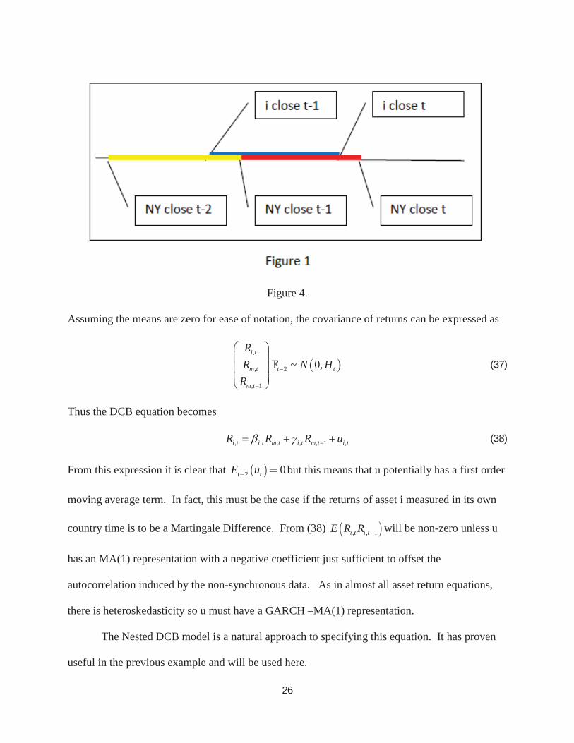
Figure 4.
Assuming the means are zero for ease of notation, the covariance of returns can be expressed as
,
, 2
, 1
~ 0,i t
m t t t
m t
RR N H
R (37)
Thus the DCB equation becomes
, , , , , 1 ,i t i t m t i t m t i tR R R u (38)
From this expression it is clear that 2 0t tE u but this means that u potentially has a first order
moving average term. In fact, this must be the case if the returns of asset i measured in its own
country time is to be a Martingale Difference. From (38) , , 1i t i tE R R will be non-zero unless u
has an MA(1) representation with a negative coefficient just sufficient to offset the
autocorrelation induced by the non-synchronous data. As in almost all asset return equations,
there is heteroskedasticity so u must have a GARCH –MA(1) representation.
The Nested DCB model is a natural approach to specifying this equation. It has proven
useful in the previous example and will be used here.
26
, 1 , 2 , 3 , 4 , 1i t i t m t i t m t tR R R u (39)
For each lag, there is both a fixed and a time varying component.
If global equity returns are serially independent, then an even easier expression is
available since the covariance between these two factors is zero. The expression for these
coefficients can be written as
, , , , 1 , ,
, , 1 , 1 , 1 , 1 ,
1, , ,,
, , ,
m t m t m t m t m t i t
m t m t m t m t m t i t
R R R R R Ri t
i t R R R R R R
H H H
H H H (40)
which simplifies to
, , 2 , , 1 2, ,2 2
, 2 , 1 2
,i t m t t i t m t ti t i t
m t t m t t
E R R F E R R F
E R F E R F (41)
The expected return of firm i when the market is in decline is called the Marginal
Expected Shortfall or MES and is defined as
, 1 , ,i t t i t m tMES E R R c (42)
In the asynchronous trading context with DCB, the natural generalization is to consider the loss
on two days after the global market declines on one day. The answer is approximately the sum
of beta and gamma from equation (38) times the Expected Shortfall of the global market.
2 , , 1 ,
2 , 1 , 1 , 1 , , , , , 1 ,
2 , 1 , 2 , ,
, , 1 , ,
t i t i t m t
t i t m t i t m t i t m t i t m t m t
t i t i t t m t m t
i t i t t m t m t
MES E R R R c
E R R R R R c
E E R R c
E R R c
(43)
The last approximation is based on the near unit root property of all these coefficients when
examined on a daily basis.
27
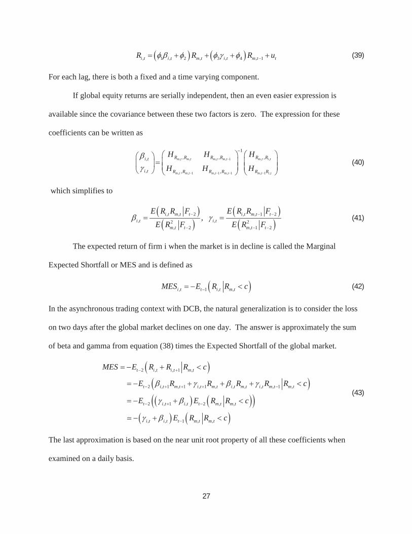
This statistical model is now operating in V-LAB where it computes SRISK for 1200
global financial institutions weekly and ranks them. Plots of the betas of the four highest SRISK
European banks will serve to illustrate the effectiveness of the DCB model. In each case the beta
is the sum of the current and the lagged beta.
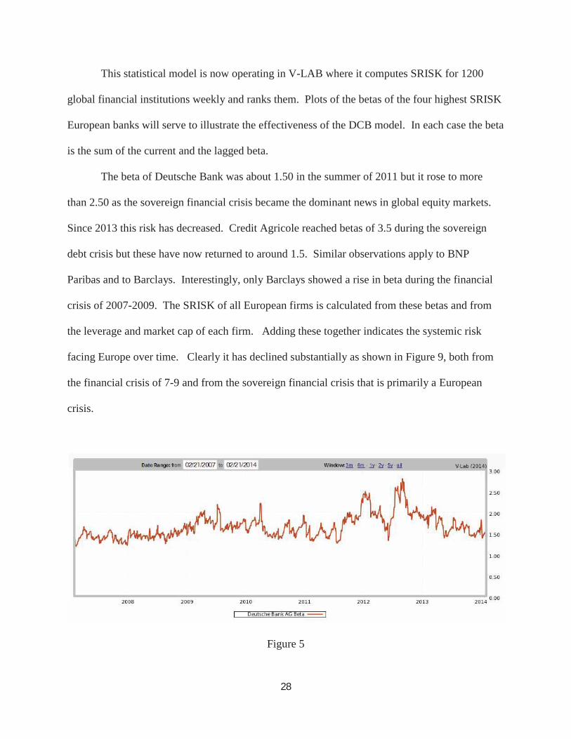
The beta of Deutsche Bank was about 1.50 in the summer of 2011 but it rose to more
than 2.50 as the sovereign financial crisis became the dominant news in global equity markets.
Since 2013 this risk has decreased. Credit Agricole reached betas of 3.5 during the sovereign
debt crisis but these have now returned to around 1.5. Similar observations apply to BNP
Paribas and to Barclays. Interestingly, only Barclays showed a rise in beta during the financial
crisis of 2007-2009. The SRISK of all European firms is calculated from these betas and from
the leverage and market cap of each firm. Adding these together indicates the systemic risk
facing Europe over time. Clearly it has declined substantially as shown in Figure 9, both from
the financial crisis of 7-9 and from the sovereign financial crisis that is primarily a European
crisis.
Figure 5
28
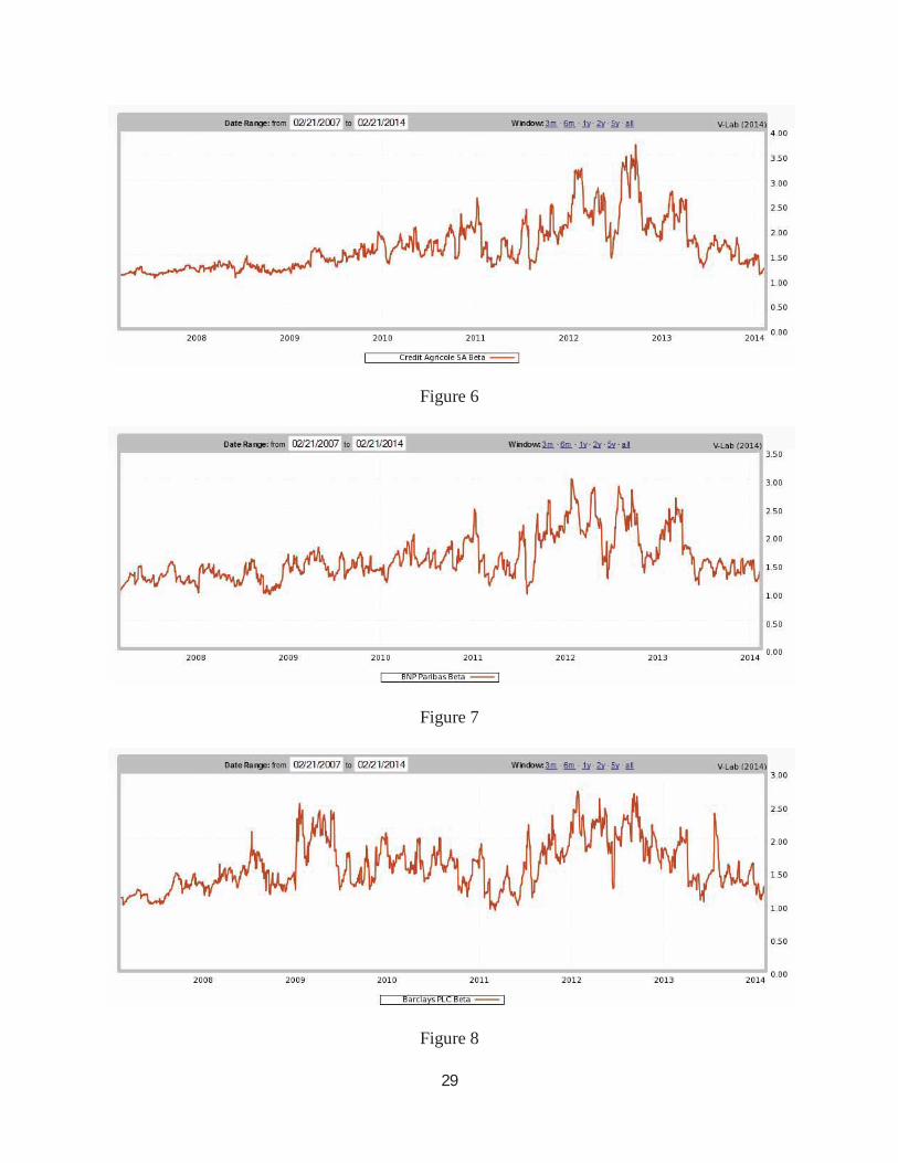
Figure 6
Figure 7
Figure 8
29
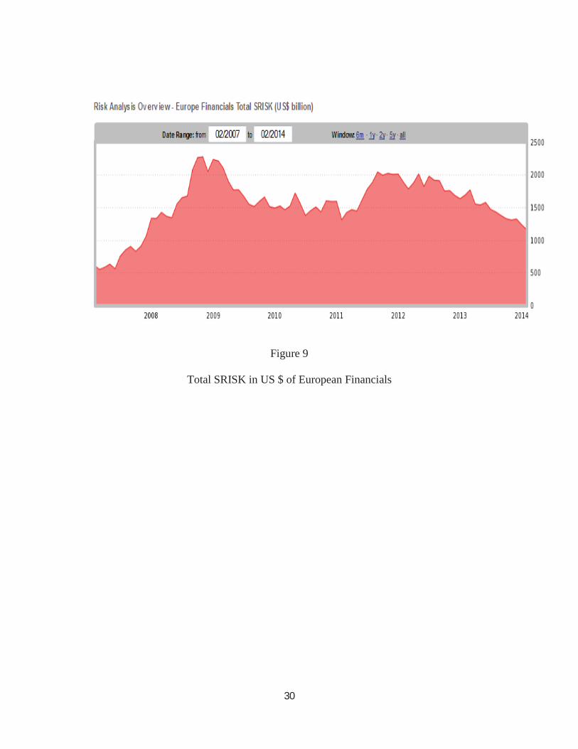
Figure 9
Total SRISK in US $ of European Financials
30
IX Conclusion
This paper has introduced a new method to estimate time series regressions that allow for
time variation in the regression coefficients called Dynamic Conditional Beta or DCB. The
approach makes clear that the regression coefficient should be based on the predicted
covariances of endogenous and exogenous variables as well as potentially the predicted means.
Estimation of the model is discussed in a likelihood context with some betas varying and others
constant. Testing the constancy of beta is a non-nested hypothesis and several approaches are
suggested and implemented. The most attractive appears to be artificial nesting which motivates
the NESTED DCB model where both constant and time varying coefficients are introduced.
The model is applied in two contexts, multi-factor asset pricing and systemic risk
assessment. The Fama French three factor model is applied to industry portfolios and the fixed
beta assumption is tested. There is strong evidence that the betas are time varying. From plots it
is apparent that the HML beta is the most volatile. In the global systemic risk context a dynamic
two factor model is estimated which allows foreign equities to respond to current as well as
lagged global prices which is expected because of non-synchronous markets. As a result, betas
for global financial institutions can be followed over time. The big European banks have had
rising betas over the fall of 2011 as the sovereign debt crisis grows in strength. This is an input
to the NYU Stern Systemic Risk Ranking displayed on V-LAB which documents the serious
nature of systemic risk in 2012 and its improvement in 2013.
31
REFERENCES
Acharya, V. V., L.H. Pedersen, T. Philippon, and M.P. Richardson. 2010, “Measuring Systemic Risk.” In V.V. Acharya, T. Cooley, M. Richardson, and I. Walter (eds.), Regulating Wall Street: The Dodd-Frank Act and the New Architecture of Global Finance. Hoboken, NJ: John Wiley & Sons, Inc.
Acharya V.V., R.F. Engle, and M.P. Richardson. 2012. Capital Shortfall: A New Approach to Ranking and Regulating Systemic Risks,” Papers and Proceedings of American Economic Review 102(3): 59-64.
Andersen, T.G., T. Bollerslev, F.X. Diebold, and J. Wu. 2006. “Realized Beta: Persistence and Predictability.” In T. Fomby and D. Terrell (eds.), Advances in Econometrics: Econometric Analysis of Economic and Financial Time Series in Honor of R.F. Engle and C.W.J. Granger,vol. B. Oxford, UK: Elsevier Ltd.
Atkinson, A. 1970. A method for discriminating between models. Journal of the Royal Statistical Society B(32): 323–53.
Bali, T.G. and R.F. Engle. 2010. The Intertemporal Capital Asset Pricing Model with Dynamic Conditional Correlations. Journal of Monetary Economics 57(4): 377-390.
Bali, T.G., R.F. Engle, and Y. Tang. 2012. “Dynamic Conditional Beta is Alive and Well in the Cross-Section of Daily Stock Returns.” Manuscript, Georgetown University.
Ball, R., and S.P. Kothari. 1989. Nonstationary expected returns: Implications for tests of market efficiency and serial correlation in returns. Journal of Financial Economics 25: 51-74.
Barndorff-Nielson, O., P.R. Hansen, A. Lunde, and N. Shephard. 2011. Multivariate Realised Kernels: Consistent Positive Semi-Definite Estimators of the Covariation of Equity Prices with Noise and Non-Synchronous Trading. Journal of Econometrics 162: 149-169.
Bera, A.K., and M.L. Higgins. 1993. ARCH Models: Properties, Estimation and Testing. Journalof Economic Surveys 7: 305-366.
Bera, A.K., and M.L. Higgins. 1998. “A Survey of ARCH Models.” In R. Jarrow (ed.), Volatility: New Techniques for Pricing Derivatives and Managing Financial Portfolios. Risk Publications.
Bera, A.K., P. Garcia, and J-S. Roh. 1998. Estimation of Time-Varying Hedge Ratios for Corn and Soybeans: BGARCH and Random Coefficient Approaches. Sankhya 59:346-368.
Bollerslev, T., R.F. Engle, and J. Wooldridge. 1988. A Capital Asset Pricing Model with Time-Varying Covariances. Journal of Political Economy 96(1): 116-131.
32
Bollerslev, T., and J. Wooldridge. 1992. Quasi-Maximum Likelihood Estimation and Inference in Dynamic Models with Time Varying Covariances. Econometric Reviews 11(2): 143-172.
Bollerslev, T., R.Y. Chou, and K.F. Kroner. 1992. ARCH Modeling in Finance: A Review of the Theory and Empirical Evidence. Journal of Econometrics 52(1): 5-59.
Bollerslev, T., R.F. Engle, and D.B. Nelson. 1994. "ARCH Models." In R.F. Engle and D. McFadden (eds.), Handbook of Econometrics, vol. IV. Amsterdam: North-Holland.
Bollerslev, T., F.X. Diebold, and Wu, J. 2005. “Realized Beta: Persistence and Predictability.” In T. Fomby (ed.), Advances in Econometrics: Econometric Analysis of Economic and Financial Time Series, vol. B. Amsterdam: Elsevier Science B.V.
Braun, P.A., D.B. Nelson, and A.M. Sunier. 1995. Good News, Bad News, Volatility, and Betas. The Journal of Finance 50: 1575-1603.
Brownlees, C., and R.F. Engle. 2011. “Volatility, Correlation and Tails for Systemic Risk Measurement.” Working Paper, Department of Finance, New York University.
Burns, P., R.F. Engle, and J. Mezrich. 1998. Correlations and Volatilities of Asynchronous Data. Journal of Derivatives 5(4): 7-18.
Cecchetti, S.G., R.E. Cumby, and S. Figlewski. 1988. “Estimation of the Optimal Futures Hedge.” Review of Economics and Statistics 70: 623-630.
Cox, D. R. 1961. Tests of Separate Families of Hypothesis. Proceedings of the Forth Berkeley Symposium on Mathematical Statistics and Probability 1: 105–23.
Cox, D. R. 1962. Further Results on Tests of Separate Families of Hypothesis. Journal of the Royal Statistical Society B(24): 406–24.
Engle, R.F., D. Hendry, and J.F. Richard. 1983. Exogeneity. Econometrica 51(2): 277-304.
Engle, R.F. 2002. Dynamic Conditional Correlation: A Simple Class of Multivariate Generalized Autoregressive Conditional Heteroskedasticity Models. Journal of Business and Economic Statistics 20: 339-350.
Engle, R.F. 2009. Anticipating Correlations: A New Paradigm for Risk Management. Princeton,NJ: Princeton University Press.
Engle, R.F., C. Pakel, N. Shephard, and K. Sheppard. 2014. “Fitting Vast Dimensional Time-Varying Covariance Models.” Manuscript.
Fama, E., and K. French. 2004. The Capital Asset Pricing Model: Theory and Evidence. Journalof Economic Perspectives 18(3): 25-46.
33
French, K.R. 2014. “Current Research Returns.”http://mba.tuck.dartmouth.edu/pages/faculty/ken.french/data_library.html
Kroner, K., and J. Sultan. 1993. Time-Varying Distributions and Dynamic Hedging with Foreign Currency Futures. Journal of Finance and Quantitative Analysis 28(4): 535-551.
Lien, D., Y.K. Tse, and A.K.C. Tsui. 2000. Evaluating the Hedging Performance of the Constant-Correlation GARCH Model. Applied Financial Economics 12(11): 791-798.
Lien, D., and Y.K. Tse. 2002. Some Recent Developments in Futures Hedging. Journal of Economic Surveys 16(3): 357-396.
Pagan, A. 1984. Econometric Issues in the Analysis of Regressions with Generated Regressors.International Economic Review 25(1): 221-247.
Patton, A.J., and M. Verardo. 2012. Does Beta Move with News?: Firm-Specific Information Flows and Learning About Profitability. Review of Financial Studies 25(9): 2789-2839.
Rivers, D., and Q. Vuong. 2002. Model Selection Tests for Nonlinear Dynamic Models. Econometrics Journal 5: 1–39.
Vuong, Q. 1989. Likelihood Ratio Tests for Model Selection and Non-Nested Hypotheses. Econometrica 57(2): 307-333.
Wooldridge, J. 2002. Econometric Analysis of Cross Section and Panel Data. Cambridge, MA: MIT Press.
34
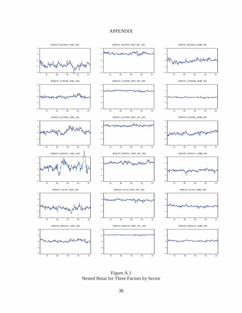
APPENDIX
Figure A.1Nested Betas for Three Factors by Sector
-2
-1
0
1
2
70 80 90 00 10
BNEST_BUSEQ_HML_SM
-2
-1
0
1
2
70 80 90 00 10
BNEST_BUSEQ_MKT_RF_SM
-2
-1
0
1
2
70 80 90 00 10
BNEST_BUSEQ_SMB_SM
-2
-1
0
1
2
70 80 90 00 10
BNEST_CHEMS_HML_SM
-2
-1
0
1
2
70 80 90 00 10
BNEST_CHEMS_MKT_RF_SM
-2
-1
0
1
2
70 80 90 00 10
BNEST_CHEMS_SMB_SM
-2
-1
0
1
2
70 80 90 00 10
BNEST_DURBL_HML_SM
-2
-1
0
1
2
70 80 90 00 10
BNEST_DURBL_MKT_RF_SM
-2
-1
0
1
2
70 80 90 00 10
BNEST_DURBL_SMB_SM
-2
-1
0
1
2
70 80 90 00 10
BNEST_ENRGY_HML_SM
-2
-1
0
1
2
70 80 90 00 10
BNEST_ENRGY_MKT_RF_SM
-2
-1
0
1
2
70 80 90 00 10
BNEST_ENRGY_SMB_SM
-2
-1
0
1
2
70 80 90 00 10
BNEST_HLTH_HML_SM
-2
-1
0
1
2
70 80 90 00 10
BNEST_HLTH_MKT_RF_SM
-2
-1
0
1
2
70 80 90 00 10
BNEST_HLTH_SMB_SM
-2
-1
0
1
2
70 80 90 00 10
BNEST_MANUF_HML_SM
-2
-1
0
1
2
70 80 90 00 10
BNEST_MANUF_MKT_RF_SM
-2
-1
0
1
2
70 80 90 00 10
BNEST_MANUF_SMB_SM
35
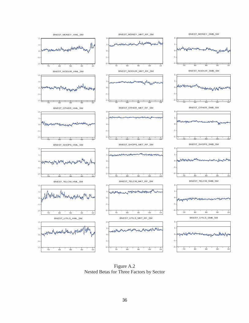
Figure A.2Nested Betas for Three Factors by Sector
-2
-1
0
1
2
70 80 90 00 10
BNEST_MONEY_HML_SM
-2
-1
0
1
2
70 80 90 00 10
BNEST_MONEY_MKT_RF_SM
-2
-1
0
1
2
70 80 90 00 10
BNEST_MONEY_SMB_SM
-2
-1
0
1
2
70 80 90 00 10
BNEST_NODUR_HML_SM
-2
-1
0
1
2
70 80 90 00 10
BNEST_NODUR_MKT_RF_SM
-2
-1
0
1
2
70 80 90 00 10
BNEST_NODUR_SMB_SM
-2
-1
0
1
2
70 80 90 00 10
BNEST_OTHER_HML_SM
-2
-1
0
1
2
70 80 90 00 10
BNEST_OTHER_MKT_RF_SM
-2
-1
0
1
2
70 80 90 00 10
BNEST_OTHER_SMB_SM
-2
-1
0
1
2
70 80 90 00 10
BNEST_SHOPS_HML_SM
-2
-1
0
1
2
70 80 90 00 10
BNEST_SHOPS_MKT_RF_SM
-2
-1
0
1
2
70 80 90 00 10
BNEST_SHOPS_SMB_SM
-2
-1
0
1
2
70 80 90 00 10
BNEST_TELCM_HML_SM
-2
-1
0
1
2
70 80 90 00 10
BNEST_TELCM_MKT_RF_SM
-2
-1
0
1
2
70 80 90 00 10
BNEST_TELCM_SMB_SM
-2
-1
0
1
2
70 80 90 00 10
BNEST_UTILS_HML_SM
-2
-1
0
1
2
70 80 90 00 10
BNEST_UTILS_MKT_RF_SM
-2
-1
0
1
2
70 80 90 00 10
BNEST_UTILS_SMB_SM
36