Dynamic Curves Are Reliable Predictors of Naturalistic

Dynamic I-V Curves Are Reliable Predictors of NaturalisticPyramidal-Neuron Voltage Traces

Laurent Badel,1 Sandrine Lefort,2 Romain Brette,3 Carl C. H. Petersen,2 Wulfram Gerstner,1

and Magnus J. E. Richardson1,4

1Laboratory of Computational Neuroscience, School of Computer and Communication Sciences and Brain Mind Institute and 2Laboratoryof Sensory Processing, Brain Mind Institute, Ecole Polytechnique Federale de Lausanne (EPFL), Lausanne, Switzerland; 3Equipe Odyssee,Departement d’Informatique, Ecole Normale Superieure, Paris, France; and 4Warwick Systems Biology Centre, University of Warwick,Coventry, United Kingdom

Submitted 5 October 2007; accepted in final form 3 December 2007

Badel L, Lefort S, Brette R, Petersen CC, Gerstner W, Richard-son MJ. Dynamic I-V curves are reliable predictors of naturalisticpyramidal-neuron voltage traces. J Neurophysiol 99: 656–666, 2008.First published December 5, 2007; doi:10.1152/jn.01107.2007. Neu-ronal response properties are typically probed by intracellular mea-surements of current-voltage (I-V) relationships during application ofcurrent or voltage steps. Here we demonstrate the measurement of anovel I-V curve measured while the neuron exhibits a fluctuatingvoltage and emits spikes. This dynamic I-V curve requires only a fewtens of seconds of experimental time and so lends itself readily to therapid classification of cell type, quantification of heterogeneities incell populations, and generation of reduced analytical models. Weapply this technique to layer-5 pyramidal cells and show that theirdynamic I-V curve comprises linear and exponential components,providing experimental evidence for a recently proposed theoreticalmodel. The approach also allows us to determine the change ofneuronal response properties after a spike, millisecond by millisecond,so that postspike refractoriness of pyramidal cells can be quantified.Observations of I-V curves during and in absence of refractoriness arecast into a model that is used to predict both the subthreshold responseand spiking activity of the neuron to novel stimuli. The predictions ofthe resulting model are in excellent agreement with experimentaldata and close to the intrinsic neuronal reproducibility to repeatedstimuli.

I N T R O D U C T I O N

Accurate models of electrically active cells and their inter-actions are central requirements for the understanding ofthe computational processes taking place in nervous tissue. Theconstruction of network models, even at the level of corticalcolumns, requires the identification of cell classes and thequantification of both their typical behavior and the heteroge-neities within a population. The volume of data that is requiredfor this tissue-level modeling demands a high-throughput ap-proach in which response properties can be routinely mea-sured.

Electrophysiology provides an array of techniques for theextraction of neuronal response properties. Standard methodsinvolve probing the response to step-change stimuli leading tocurrent-voltage (I-V) curves for the steady-state or instanta-neous response. Used systematically with pharmacology, theycan yield a full conductance-based description (Hodgkin andHuxley 1952; Koch 1999) although the time required is pro-

hibitive for routine neuron-by-neuron classification. More re-cently, an elegant optimization method (Huys et al. 2006) hasbeen proposed that promises to significantly facilitate theconstruction of biophysically detailed models, given someprior knowledge of the kinetics of the channels present.

Detailed models, comprising hundreds of compartments, areimportant for understanding the biophysical properties probedduring electrophysiological and pharmacological manipula-tions. Such models can be used for network simulations onhigh-performance computers, but the complexity associatedwith a high level of detail means that it can be difficult to geta deep understanding of the network states that emerge in thesesimulations. At the other end of the spectrum of neuron modelsare single-variable integrate-and-fire type models. The mathe-matical analysis of this class of models has given a great dealof insight into the emergence of dynamic network states(Abbott and van Vreeswijk 1993; Brunel and Hakim 1999;Gerstner 2000; Gerstner and van Hemmen 1993), and they arereadily extended to include further biological details such assubthreshold currents (Brunel et al. 2003; Richardson et al.2003) and adaptation (Gigante et al. 2007).

An interesting link can be made between one-variable mod-els and I-V curves; both involve the reduction of multi-variabledynamics, comprising voltage and channel activation states, toa relation between the net membrane current and voltage.Standard stimuli used for measuring I-V curves comprisestep-change current and voltage pulses (Hodgkin et al. 1952) orslow voltage ramps (see, for example, Swensen and Marder2000). However, if a more naturalistic stimulus were used togenerate an I-V curve, then a reduced model derived from thatI-V curve could provide a more efficient description of theneuronal dynamics. Ultimately the success or not of such amethod should be judged by the extent to which it can predictexperimental data.

Here we introduce a method that measures the I-V curveduring ongoing activity. An attractive feature is that it can beused to measure response properties in time slices triggered toevents in the voltage trace—an aspect that will be used toquantify the refractory properties of pyramidal cells. A modelderived from the I-V curve measurements will then be testedagainst novel stimuli, which were not used for parameterextraction, and its predictive power evaluated.

Address for reprint requests and other correspondence: M.J.E. Richardson,Warwick Systems Biology Centre, University of Warwick, CV4 7AL, Cov-entry, UK (E-mail: [email protected]).

The costs of publication of this article were defrayed in part by the paymentof page charges. The article must therefore be hereby marked “advertisement”in accordance with 18 U.S.C. Section 1734 solely to indicate this fact.

J Neurophysiol 99: 656–666, 2008.First published December 5, 2007; doi:10.1152/jn.01107.2007.

656 0022-3077/08 $8.00 Copyright © 2008 The American Physiological Society www.jn.org

on January 8, 2010 jn.physiology.org

Dow

nloaded from

http://jn.physiology.org

etsb

Underline

etsb

Underline

etsb

Underline

etsb

Underline

etsb

Underline

M E T H O D S

Slice preparation and whole cell recordings

Parasagittal neocortical brain slices (300 !m thick) from C57/B16Jmice (P12–14, n ! 8 and P20, n ! 4) were prepared using avibratome (Leica VT1000 S, Leica Microsystems GmbH, Germany)in ice-cold extracellular medium (ACSF; containing in mM: forP12–14 mice and incubation chamber, 125 NaCl, 25 NaHCO3, 25glucose, 2.5 KCl, 1.25 NaH2PO4, 2 CaCl2, and 1 MgCl2; for P20 miceslice cutting, 110 choline chloride; 25 NaHCO3; 25 D-glucose, 11.6sodium ascorbate, 7 MgCl2, 3.1 sodium pyruvate, 2.5 KCl, 1.25NaH2PO4, and 0.5 CaCl2). Slices were transferred to a chambercontaining ACSF bubbled with 95% O2-5% CO2 and incubatedat 35°C for 30 min and then at room temperature (20 –22°C) untiluse. All experiments were performed at 35°C. Pyramidal neuronswere identified by video-enhanced infrared microscopy using the20"0.95NA water-immersion lens of an upright microscope(BX51WI; Olympus, Tokyo, Japan). Double somatic whole cellrecordings were obtained from layer-5 pyramidal neurons. One pipetteinjected the current while the voltage was measured simultaneouslyfrom both. However, a two-electrode protocol for the measurement ofintracellular voltage during current injection is not necessary if anactive electrode compensation (AEC) technique (Brette et al. 2005,2007a,b) is used that digitally removes the artifacts introduced by theelectrode filter using a Wiener-Hopf optimal filtering. A review of thismethod, and the particular optimization principle used here, togetherwith the comparison between single and dual electrode recordings canbe found in APPENDIX B. The injected current waveforms wereconstructed from two summed Ornstein-Uhlenbeck processes (seeAPPENDIX A for details) with time constants "fast ! 3 ms and "slow !10 ms. There were two sets of variances (low, #fast ! #slow ! 0.18and high, #fast ! 0.36, #slow ! 0.25) and four sets of DC biases 0.0,0.02, 0.03, and 0.06 in relative units, yielding a total of 8 combina-tions of waveforms. Each waveform had a duration of 40 s and waspreceded and followed by a 3-s null (0 current) stimulus used tomeasure background noise levels. The set of eight waveforms wasinjected twice at an interval of 15 min to test for the intrinsicreliability of the cells as well as to check the stability of the cellularproperties over the duration of the recordings. To produce an averagefiring rate in the desired range (1–15 Hz), the waveforms weremultiplied by a factor (in the range 250–750 pA) to give the currentinjected into the neurons. All current waveforms contained squarepulses at the beginning and end of experiment, allowing for standardmeasures of input resistance and capacitance. The intracellular solu-tion contained the following (in mM): 135 K-gluconate, 4 KCl, 4Mg-ATP, 10 Na2- phosphocreatine, 0.3 Na-GTP, and 10 HEPES(pH ! 7.3; 270 mosmol/l). Biocytin (3 mg/ml) was routinely added toallow post hoc staining of the recorded cells. Pipette capacitance wascompensated, and whole cell recordings with access resistance#20M$ were obtained using Multiclamp 700A amplifiers (MolecularDevices, Foster City, CA). The membrane potential was filtered at 10kHz and digitized at 20 kHz using an ITC-18 (InstruTech, PortWashington, NY). All experiments were carried out following proto-cols approved by the Swiss Federal Veterinary Office.

Mathematical model

The basic model used is the exponential integrate-and-fire (EIF)model (Fourcaud-Trocme et al. 2003), given here by Eqs. 7 and 9,which was also extended to include refractory properties by makingthe three parameters Em, 1/"m, and VT dependent on the time since thelast spike (called the rEIF model). For example, given that the lastspike occurred at time tk the value of Em was calculated as Em(t) !E m

0 % A1e&(t&tk)/"1 % A2e&(t&tk)/"2, where E m0 denotes the value of Em

obtained away from a spike. The amplitudes A1, A2 and time constants"1, "2 were obtained by fitting the set of I-V curves measured in timeslices after each output spike (see Fig. 3). For 1/"m and VT, a single

exponential term was sufficient, and a dynamics for 'T was notrequired.

Equation 7 with the definition of F(V) given in Eq. 9 was integratedusing an Euler scheme with a time step corresponding to the samplingrate of the recordings (20 kHz). The action potentials of the modelappear as a rapid rise in voltage and the integration was stopped whenV reached 0 mV. Because the downswing of the spike is not explicitlydescribed in the model, the integration was interrupted for 2 ms afterdetection of an action potential (typical duration of the action potentialdownswing) and restarted at a reset Vre, which was in general close toor above the prespike threshold VT

0. The shifting of the spike initiationthreshold VT toward a more depolarized value after a spike preventsthe immediate generation of a second action potential. For the non-refractory EIF model, it was necessary to use a reset value that issufficiently subthreshold to prevent repetitive firing. For this model,Vre ! &55 mV followed by a 10-ms refractory period in all thesimulations was used.

The performance index (Jolivet et al. 2004; Kistler et al. 1997) usedto compare spike trains generated by the model to the experimentalrecordings was taken to be the coincidence factor (

( $Ncoinc % )Ncoinc*

0.5+Nmodel & Nneuron,

1

!(1)

Ncoinc is the number of coincidences with precision ' ! 5 ms,!Ncoinc" ! 2f'Nneuron is the number of expected chance coincidencesgenerated by a Poisson process with the same firing rate f asthe neuron, Nneuron and Nmodel are the number of spikes in the spiketrains of the neuron and the model, respectively (! is a normal-ization factor that is of no importance in the following as onlyratios of ( are considered). In Fig. 4B, the ratio (/(- is plotted,where ( evaluates the overlap between the prediction of the modeland a target experimental spike train, and (- is calculated betweenthe target spike train and a second experimental recording obtainedwith the same driving current. Only pairs of trials with an exper-imental reliability (- . 0.75 between recording sessions spaced by15 min were used. Setting the threshold at this level still includedneurons that fire at low rates (around 1 Hz) but excluded those inwhich a significant drift in cellular properties (significantly in-creasing or decreasing voltage baselines or firing rates) was seenover the time between the repeated measurements.

R E S U L T S

To produce fluctuating voltage traces, a stochastic currentwas injected into somatosensory pyramidal cells via a wholecell somatic patch-clamp electrode. Basic electrophysiologyprovides an equation that relates the capacitive charging cur-rent and the summed effect Im(V, t) of the transmembranecurrents to this injected current Iin(t)

CdV

dt& Im+V, t, & Inoise $ Iin +t, (2)

In this formulation, Im comprises both transmembrane cur-rents and equilibrating currents flowing between the soma(point of current injection) and the dendrites and axon. Thenoise term Inoise comprises effects from weak backgroundsynaptic activity and other sources of high-frequency variabil-ity. Equation 2 may be re-arranged to yield the dynamictransmembrane current

Im +V, t, & Inoise $ Iin +t, % CdV

dt(3)

The injected current waveform Iin is known a priori and thederivative dV/dt may be calculated from the experimentally

657DYNAMIC I-V CURVES OF LAYER-5 PYRAMIDAL CELLS

J Neurophysiol • VOL 99 • FEBRUARY 2008 • www.jn.org


Dow

nloaded from


etsb

Underline

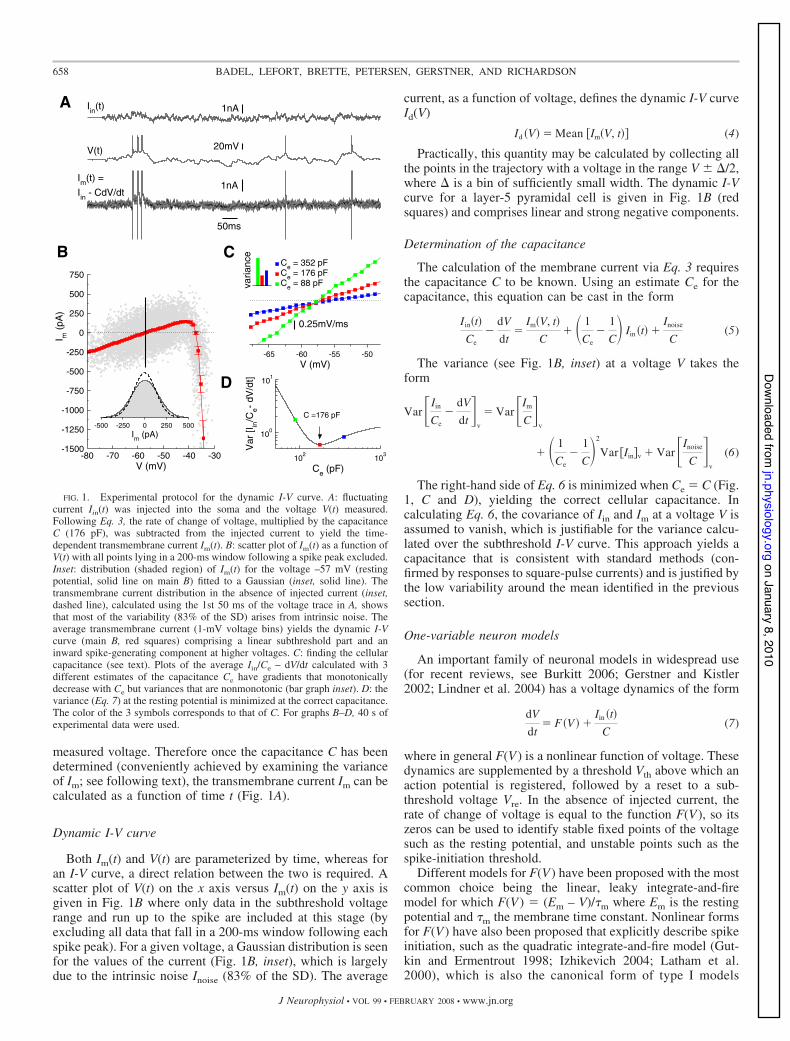
measured voltage. Therefore once the capacitance C has beendetermined (conveniently achieved by examining the varianceof Im; see following text), the transmembrane current Im can becalculated as a function of time t (Fig. 1A).

Dynamic I-V curve

Both Im(t) and V(t) are parameterized by time, whereas foran I-V curve, a direct relation between the two is required. Ascatter plot of V(t) on the x axis versus Im(t) on the y axis isgiven in Fig. 1B where only data in the subthreshold voltagerange and run up to the spike are included at this stage (byexcluding all data that fall in a 200-ms window following eachspike peak). For a given voltage, a Gaussian distribution is seenfor the values of the current (Fig. 1B, inset), which is largelydue to the intrinsic noise Inoise (83% of the SD). The average

current, as a function of voltage, defines the dynamic I-V curveId(V)

Id +V, $ Mean /Im+V, t,0 (4)

Practically, this quantity may be calculated by collecting allthe points in the trajectory with a voltage in the range V 1 '/2,where ' is a bin of sufficiently small width. The dynamic I-Vcurve for a layer-5 pyramidal cell is given in Fig. 1B (redsquares) and comprises linear and strong negative components.

Determination of the capacitance

The calculation of the membrane current via Eq. 3 requiresthe capacitance C to be known. Using an estimate Ce for thecapacitance, this equation can be cast in the form

Iin+t,

Ce%

dV

dt$

Im+V, t,

C& # 1

Ce%

1

C$ Iin +t, &Inoise

C(5)

The variance (see Fig. 1B, inset) at a voltage V takes theform

Var%Iin

Ce%

dV

dt &v

$ Var%Im

C&v

& # 1

Ce%

1

C$2

Var /Iin0v & Var%Inoise

C &v

(6)

The right-hand side of Eq. 6 is minimized when Ce ! C (Fig.1, C and D), yielding the correct cellular capacitance. Incalculating Eq. 6, the covariance of Iin and Im at a voltage V isassumed to vanish, which is justifiable for the variance calcu-lated over the subthreshold I-V curve. This approach yields acapacitance that is consistent with standard methods (con-firmed by responses to square-pulse currents) and is justified bythe low variability around the mean identified in the previoussection.

One-variable neuron models

An important family of neuronal models in widespread use(for recent reviews, see Burkitt 2006; Gerstner and Kistler2002; Lindner et al. 2004) has a voltage dynamics of the form

dV

dt$ F +V , &

Iin +t,

C(7)

where in general F(V ) is a nonlinear function of voltage. Thesedynamics are supplemented by a threshold Vth above which anaction potential is registered, followed by a reset to a sub-threshold voltage Vre. In the absence of injected current, therate of change of voltage is equal to the function F(V ), so itszeros can be used to identify stable fixed points of the voltagesuch as the resting potential, and unstable points such as thespike-initiation threshold.

Different models for F(V ) have been proposed with the mostcommon choice being the linear, leaky integrate-and-firemodel for which F(V ) ! (Em – V)/"m where Em is the restingpotential and "m the membrane time constant. Nonlinear formsfor F(V ) have also been proposed that explicitly describe spikeinitiation, such as the quadratic integrate-and-fire model (Gut-kin and Ermentrout 1998; Izhikevich 2004; Latham et al.2000), which is also the canonical form of type I models

Iin(t) 1nA

V(t) 20mV

Im(t) =Iin - CdV/dt

50ms

1nA

-500 -250 0 250 500Im (pA)

varia

nce

-65 -60 -55 -50V (mV)

0.25mV/ms

Ce = 352 pFCe = 176 pFCe = 88 pF

102 103

Ce (pF)

100

101

Var

[Iin/C

e- dV

/dt]

C =176 pF

-80 -70 -60 -50 -40 -30V (mV)

-1500

-1250

-1000

-750

-500

-250

0

250

500

750

I m (

pA)

A

B

D

C

FIG. 1. Experimental protocol for the dynamic I-V curve. A: fluctuatingcurrent Iin(t) was injected into the soma and the voltage V(t) measured.Following Eq. 3, the rate of change of voltage, multiplied by the capacitanceC (176 pF), was subtracted from the injected current to yield the time-dependent transmembrane current Im(t). B: scatter plot of Im(t) as a function ofV(t) with all points lying in a 200-ms window following a spike peak excluded.Inset: distribution (shaded region) of Im(t) for the voltage –57 mV (restingpotential, solid line on main B) fitted to a Gaussian (inset, solid line). Thetransmembrane current distribution in the absence of injected current (inset,dashed line), calculated using the 1st 50 ms of the voltage trace in A, showsthat most of the variability (83% of the SD) arises from intrinsic noise. Theaverage transmembrane current (1-mV voltage bins) yields the dynamic I-Vcurve (main B, red squares) comprising a linear subthreshold part and aninward spike-generating component at higher voltages. C: finding the cellularcapacitance (see text). Plots of the average Iin/Ce – dV/dt calculated with 3different estimates of the capacitance Ce have gradients that monotonicallydecrease with Ce but variances that are nonmonotonic (bar graph inset). D: thevariance (Eq. 7) at the resting potential is minimized at the correct capacitance.The color of the 3 symbols corresponds to that of C. For graphs B–D, 40 s ofexperimental data were used.

658 BADEL, LEFORT, BRETTE, PETERSEN, GERSTNER, AND RICHARDSON



Dow

nloaded from


(Ermentrout 1996; Ermentrout and Kopell 1986). An alter-native proposal for the nonlinearity is the EIF model(Fourcaud-Trocme et al. 2003) that includes the activationof the spike-generating sodium current. It has been shown(Fourcaud-Trocme and Brunel 2005) that the functionalform used to model the spike-initiation is a crucial determi-nant of the neuronal response to rapid synaptic signaling.

The dynamic I-V curve provides an experimental method formeasuring F(V ) directly. On comparing Eqs. 2 and 7, a naturalinterpretation is

F +V , $ %Id+V,/C (8)

where Id was defined in Eq. 4. With this choice, the intrinsiccurrent of the model will be the same as in the experimentaldata on average. Although the temporal effects of voltage-gated currents are averaged out in this one-variable (somaticvoltage) model, it was shown in the previous section that afterthe intrinsic variability is accounted for, the unexplained vari-ability around the mean is low, so it can be expected that Eq.8 would have the potential to provide an accurate description ofneuronal dynamics.

In Fig. 2A, the function F(V ) (expansion of data in Fig. 1B)measured from a pyramidal cell is plotted (symbols). There aretwo fixed points where F(V ) ! 0 for the resting potential andspike-initiation threshold, a linear region where the cellularresponse is passive and a rapid nonlinear component at highervoltages. A semi-log plot (see inset) shows that the nonlinearcomponent is exponential (y axis), and therefore these mea-surements provide convincing empirical evidence for the EIFmodel (Fourcaud-Trocme et al. 2003) for pyramidal cells forwhich

F +V, $1

"m#Em % V & 'T exp#V % VT

'T$$ (9)

The EIF model has four parameters: the membrane timeconstant "m, the resting potential Em, the spike-initiationthreshold VT, and the spike width 'T, which controls thesharpness of the initial phase of the spike. A least-squares fitof the full form of Eq. 9 to the pyramidal-cell I-V curve data(Fig. 2A, solid line) is seen to be in excellent agreement withthe pyramidal-cell dynamic I-V curve. It should be noted thatthe spike initiation for pyramidals is sharper than that of thehippocampal interneuron model (Wang and Buzsaki 1996) usedin the original EIF paper (Fourcaud-Trocme et al. 2003) incommon with the “kink”-like spikes identified in recent ana-lyzes of pyramidal-cell voltage recordings (McCormick et al.2007; Naundorf et al. 2006).

Variation across the population

By comparing the results from different recordings (n ! 12),we found that the qualitative shape of the dynamic I-V curvewas remarkably stable across layer-5 pyramidals with theEIF model always providing an excellent match. Afterfitting the model to data on a neuron-by-neuron basis, weexamined the histograms of model parameters (Fig. 2B).The coefficients of variation (CV) for the membrane timeconstant, distance to threshold and spike width were 32, 25,and 33%, respectively, demonstrating a significant degree ofheterogeneity in the population, with implications for net-work modeling.

Postspike curve

The dynamic I-V method can also be applied to transientchanges in response properties, such as the postspike recoveryperiod excluded from the treatment illustrated in Figs. 1 and 2.To this end, we separated the postspike data into the time slicesshown in Fig. 3A, and for each time slice, the dynamic I-Vcurve was again calculated. The resulting postspike I-V curvesare quantitatively different and relax to the prespike form overa period of many tens of milliseconds. The EIF functional form(Eq. 9) also provided a good fit to the postspike data, whichwas unexpected, allowing for the refractory properties to bequantified in terms of the dynamic effects on the EIF param-eters (Fig. 3B). The dynamics of the parameters could be fittedby a single exponential term except for the resting potential Em(requiring a biexponential form), which showed a prominentsag indicative of the transient activation of a hyperpolariz-ing current or of the deactivation of a depolarizing current,such as Ih.

Verification of the models

These pre- and postspike response properties were used toconstruct two models which were tested against further exper-iments. The first model comprises Eqs. 7 and 9 with a “hard”subthreshold postspike reset and is identical to the EIF model(Fourcaud-Trocme et al. 2003). The second is a novel refrac-

-80 -70 -60 -50 -40 -30V (mV)

-1

0

1

2

3

4

5

6

7

8

F(V

) (m

V/m

s)

fit to EIF modeldynamic IV data

-40 -30 -20 -10 0 10 20 30V

0.1

1

10

100

F(V

) -

(Em

-V)/τ

m

0 20 40 60τm (ms)

-70 -60 -50 -40Em (mV)

0 10 20 30VT - Em (mV)

0 1 2 3∆T (mV)

A

B

resting potential spike initiation

FIG. 2. Quantification of the dynamic I-V curve. A: the experimentallymeasured I-V curve [plotted with the sign inverted to yield the function F(V ),symbols] plotted together with the exponential integrate-and-fire (EIF) modelfit (line) with parameters "m ! 17.2 ms, Em ! &57.0 mV, VT ! &42.0 mV,and 'T ! 1.51 mV. The curve crosses the V axis at 2 voltages: &57 mV(resting potential) and –38 mV (spike-initiation threshold). Inset: semi-log plotof the I-V curve and fit (with linear component subtracted) during the upswingof the action potential showing a clear exponential rise (fit with the exponentialup to –30 mV followed by a rounding-off of the action potential around itspeak value of %30 mV). B: the distributions of the EIF parameters for a sampleof pyramidal cells (n ! 12) with means 1 SD: "m ! 23.3 1 7.5 ms, Em !&57.8 1 4.4 mV, VT – Em ! 12.6 1 3.2 mV, and 'T ! 1.2 1 0.4 mV. Thecapacitance (data not shown), which is a function of cell geometry and size,also varied across the population with C ! 260 1 75 pF.




Dow

nloaded from


tory EIF model (rEIF) for which the “soft” refractory periodrelaxes with the dynamics identified in Fig. 3 (see METHODS).

For each cell investigated, a range of test currents, withdifferent means and variances, were injected to produce volt-age traces with firing rates in the range of 1–15 Hz. A uniqueset of model parameters was extracted individually for eachcell via a fit to the dynamic I-V curve from a single 40-s voltagetrace of intermediate firing rate (for the nonrefractory model,the voltage data in a 200-ms window following each spike peakwere excluded from the analysis). The parameters of thismodel were then fixed to be tested on the other currentwaveforms and compared with the response from the samecell. Each test current was injected into the cell twice so thatthe intrinsic reliability of the cell could also be quantified. Themeasures of the quality of prediction of the rEIF and EIFmodels and the cellular reliability, comprised: the averagefiring rate, the number of predicted spikes (within 15 ms of thespike peak) and the accuracy of the subthreshold voltage. Forthe latter, the root-mean-square (RMS) difference between themodel voltage and the experimental voltage was examinedusing data at least 150 ms away from spikes. For the voltagedistributions, only data between 0.5 ms before and 3 ms afterthe spike were excluded. The results are plotted in Fig. 4.

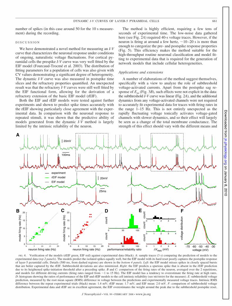
Both models predict the positions of isolated spikesaccurately and have a subthreshold voltage in close agree-ment with the experimental data. However, the hard reset ofthe EIF is a poor model of the postspike behavior of layer-5

pyramidal cells. In Fig. 4A, bottom, the EIF is seen to missa spike in a closely spaced pair (left) and to add a spuriousspike due to an underestimation of the threshold (right). Atthese firing rates, such effects were relatively rare and bothmodels matched the firing rates well (Fig. 4, B and C)although with the EIF predicting a weak excess of spikes athigher rates. The positions of the spikes were also accu-rately predicted (see METHODS) where for the rEIF in Fig. 4D,it is seen that the model rarely predicts #75% of the spikescorrectly with a mean 1 SD of 83 1 8% and where the EIFmodel has a mean 1 SD of 72 1 14% spikes predictedrelative to the intrinsic reliability. Finally, the typical RMSdifference of the subthreshold voltage for the rEIF modelwas 1.7 mV and for the EIF 2.0 mV, both of which againcompare favorably with the RMS for repeated stimuli at 1.4mV as can be seen in Fig. 4E, as well as in F, whichcompares the voltage distributions themselves.

Efficiency of the method

The results presented so far were obtained from 40-s voltagetraces. To compare the results against those from shorterrecordings, we compared the I-V curves obtained by using onlythe first 10 s of data with those obtained using the whole 40-strace. We found little difference between the model fits for thetwo recording durations (Fig. 5). It can be noted that thelimiting factor for a clean fit is the collection of a sufficient

0 0.2 0.4(1/ms)

0 20 40(ms)

0 100 200 300post-spike time (ms)

-62-60-58-56-54-52-50-48

Em

(mV

)

-50 0 50(mV)


-45

-40

-35

-30

-25

-20

VT (

mV

)

0 50 100(ms)

0 20 40(mV)


0

1

2

3

4

5

∆ T (m

V)

0 20 40(ms)


0.05

0.10

0.15

1 / τ

m (

1/m

s)

-1 0 1(mV)

10 to 20 ms 20 to 30 ms 30 to 50 ms5 to 10 ms

B

A

20m

V

2ms

A τ A2 A1τ1 τ2 A τ A

FIG. 3. Using the dynamic I-V method to measure the refractory properties of layer-5 pyramidal cells. A: I-V curves measured at different times after a spike(symbols in insets) fitted to the EIF model (solid lines). At early times, the conductance (subthreshold gradient, proportional to 1/"m) is significantly increasedas are the dynamic resting potential and threshold for spike initiation (intersections with dotted line). The postspike I-V curve relaxes slowly back to the prespikecurve (dashed lines in each inset). B: dynamics of the EIF parameters (symbols) together with the fits to an exponential model (red lines, see METHODS).Immediately after the spike, the conductance is double its prespike value. The dynamics of the resting potential Em shows a nonmonotonic sag that relaxes slowly.The threshold VT is initially almost 20 mV higher than its prespike value, significantly reducing the excitability of the cell. However, the spike width 'T changedlittle after a spike. For this cell, the fitting parameters (see METHODS) were A"m&1 ! 0.05 ms&1, ""m&1 ! 20.0 ms; A1Em ! 49.8 mV, "1Em ! 32.8 ms; A2Em !&42.7 mV, "2Em ! 42.9 ms; AVT ! 18.4 mV, "VT ! 14.0 ms; A'T ! 0.02 mV, which is small enough to be neglected and implies that "'T does not have muchsignificance. The data were gathered from 175 spikes. Error bars show the SD of the parameters measured over 4 distinct voltage traces. The insets to B showthe histograms of the exponential amplitudes A and decay constants " for a population (n ! 12) of cells. The means and variances were: A"m&1 ! 0.14 1 0.10ms, ""m&1 ! 14.3 1 6.1 ms; A1Em ! 22.9 1 9.2 mV, "1Em ! 14.7 1 6.6 ms; A2Em ! &13.5 1 10.2 mV, "2Em ! 76.2 1 50.2 ms; AVT ! 13.0 1 3.9 mV, "VT! 17.7 1 4.4 ms; A'T ! 0.03 1 0.33 mV.




Dow

nloaded from


number of spikes (in this case around 50 for the 10 s measure-ment) during the recording.

D I S C U S S I O N

We have demonstrated a novel method for measuring an I-Vcurve that characterizes the neuronal response under conditionsof ongoing, naturalistic voltage fluctuations. For cortical py-ramidal cells the prespike I-V curve was very well fitted by theEIF model (Fourcaud-Trocme et al. 2003). The distribution offitting parameters for a population of cells was also given withCV values demonstrating a significant degree of heterogeneity.The dynamic I-V curve was also measured in postspike timeslices and the refractory properties quantified. An unexpectedresult was that the refractory I-V curves were still well fitted bythe EIF functional form, allowing for the derivation of arefractory extension of the basic EIF model (rEIF).

Both the EIF and rEIF models were tested against furtherexperiments and shown to predict spike times accurately withthe rEIF showing particularly close agreement with the exper-imental data. In comparison with the neuronal response torepeated stimuli, it was shown that the predictive ability ofmodels generated from the dynamic I-V method is largelylimited by the intrinsic reliability of the neuron.

The method is highly efficient, requiring a few tens ofseconds of experimental time. The low-noise data gatheredhere (see Fig. 2A) required 40-s voltage traces. However, if theneuron is firing at around a few hertz, 210–20 s is more thanenough to categorize the pre- and postspike response properties(Fig. 5). This efficiency makes the method suitable for thehigh-throughput routine neuronal classification and model fit-ting to experimental data that is required for the generation ofnetwork models that include cellular heterogeneities.

Applications and extensions

A number of elaborations of the method suggest themselves,specifically with a view to analyze the role of subthresholdvoltage-activated currents. Apart from the postspike sag re-sponse of Em (Fig. 3B), such effects were not explicit in the data:the subthreshold I-V curve was linear (Fig. 2A), and the additionaldynamics from any voltage-activated channels were not requiredto accurately fit experimental data for traces with firing rates inthe range 1–15 Hz. This is not entirely unexpected as therapidly fluctuating voltage tonically activates voltage-gatedchannels with slower dynamics, and so their effect will largelybe seen as a change of the total membrane conductance. Thestrength of this effect should vary with the different means and

20mV

100ms

0 1 2 3 4

∆VRMS (mV)

coun

t

0 5 10 15 20neuron firing rate (Hz)

0

5

10

15

20

mod

el fi

ring

rate

(H

z)

0 5 10 15 20

neuron firing rate (Hz)

0

5

10

15

20

mod

el fi

ring

rate

(H

z)

0 50 100

coun

t

0 50 100

performance/reliability ratio

coun

t

20mV

25ms

0 1 2 3 4

coun

t

0 1 2 3 4

coun

t

-70 -60 -50 -40 -30voltage (mV)

volta

ge d

istr

ibut

ion

A

B D F

experiment

rEIF model

EIF model

C E

FIG. 4. Verification of the models (rEIF green, EIF red) against experimental data (black). A: sample traces (3 s) comparing the prediction of models to theexperimental data (top 2 panels). The models predict the isolated spikes equally well, but the EIF model with its hard reset poorly captures the postspike responseof layer-5 pyramidal cells. Details (500 ms, from dashed regions) are shown in the bottom 4 panels. Left: the EIF model misses spikes in closely spaced burststhat are better captured by the rEIF. Subthreshold deviations are also minimized. Right: the EIF predicts a spurious spike that is absent in the rEIF predictiondue to its heightened spike-initiation threshold after a preceding spike. B and C: comparison of the firing rates of the neuron, averaged over the 2 repetitions,and models for different driving currents (firing rates ranged from 21 to 15 Hz). The EIF model has a tendency to overestimate the firing rate at high rates.D: histogram showing the ratios of performance of the EIF and rEIF models to the cell intrinsic reliability (see METHODS for the measure). E: subthreshold voltageprediction, measured by the root mean square (RMS) difference in voltage between the predictions and experimentally measured voltage traces. Intrinsic RMSdifference between the repeat experimental trials (black) mean: 1.4 mV; rEIF mean: 1.7 mV; and EIF mean: 2.0 mV. F: comparison of subthreshold voltagedistribution. Experimental data and rEIF are in excellent agreement, the EIF overestimates the weight around the peak due to the subthreshold postspike reset.




Dow

nloaded from


variances of the input current, though this was not significantover the range of currents used here. Nevertheless, more refinedmeasurements that could combine fluctuating current with ramps(Swensen and Marder 2000) might be used to examine thepotential effects of the h-current, persistent sodium current, orother currents that might be present. As a related point, it wouldbe simple to extend the method to the case of fluctuatingconductance injection (Destexhe et al. 2001). Although bothcurrent and conductance fluctuations lead to very similar volt-age distributions (Burkitt 2001; Richardson 2004; Richardsonand Gerstner 2005), the frequencies present in the spectrum ofthe fluctuations increases with the level of conductance (Des-texhe and Rudolph 2004). The faster temporal structure ofconductance-based input could potentially interact differentlywith the dynamics of intrinsic currents to alter the measuredresponse properties. Such an effect might be measurable inneurons with subthreshold currents with fast dynamics (withtime scales similar to the membrane time constant), but forcurrents such as Ih (with relatively slow dynamics), this effectcould be expected to be weak. Finally, coupled to dendriticrecordings or by stimulating presynaptic units simultaneously,the dynamic I-V curve may also be employed to study how theactivation of dendritic conductances affects the processing ofinformation in the soma.

Implications for neural modeling

During the last couple of years, there has been much debatein the theoretical neuroscience community concerning theappropriate minimal description of subthreshold response andspike generation. In particular, the choice of a strict voltagethreshold, as in the classical integrate-and-fire model (Lapicque1907; Stein 1967), has been critically analyzed (Fourcaud-Trocme et al. 2003), and various generalizations have beenproposed, including canonical phase models (Ermentrout 1996;

Ermentrout and Kopell 1986; Gutkin and Ermentrout 1998),quadratic, (Latham et al. 2000) and exponential (Fourcaud-Trocme et al. 2003) integrate-and-fire models. Refractory prop-erties have also been studied in several forms (Jolivet et al.2004; Kistler et al. 1997; Lindner and Longtin 2005), and theinclusion of a second, slow variable has proven effective inreproducing more complex subthreshold dynamics such asresonance (Brunel et al. 2003; Izhikevich 2004; Richardsonet al. 2003) and adaptation (Brette and Gerstner 2005; Clopathet al. 2007; Gigante et al. 2007; Jolivet et al. 2004). Thedynamical I-V curve data for cortical pyramidals, and associ-ated modeling, presented here provides clear empirical evi-dence for the EIF model (Fourcaud-Trocme et al. 2003),which, even with a hard reset, was able to give an accurateprediction of the spike times. It is interesting to note that themeasured spike width 'T for pyramidal cells is considerablysharper than that predicted from the original fits to an inter-neuron model with Hodgkin-Huxley spike-generating currents(Wang and Buzsaki 1996). Given that the leaky integrate-and-fire (IF) model is recovered from the EIF model in the limit'T3 0, this empirical result goes some way in explaining thesuccess of leaky IF models in predicting firing rates (Rauch etal. 2003) and spike times (Jolivet et al. 2006; Paninski et al.2004).

Our findings also clearly highlight the importance of refrac-tory properties for the correct modeling of cortical pyramidals.The measured refractory properties comprised conductance in-crease and, most importantly, a significantly increased thresholdfor spike initiation allowing for a postspike reset that is abovethe prespike threshold. Although the idea of exponentiallyrelaxing refractory properties is far from new (Fuortes andMantegazzini 1962; Geisler and Goldberg 1966), it has untilrecently (Chacron et al. 2007; Gerstner and van Hemmen 1993;Lindner and Longtin 2005) received little analytical attention.

0 100 200 300-62

-60

-58

-56

-54

-52

-50

-48

Em

(m

V)

0 100 200 300time following spike (ms)

-45

-40

-35

-30

-25

VT (

mV

)0 100 200 300

0

1

2

3

4

5

∆ T (

mV

)

0 100 200 3000.00

0.02

0.04

0.06

0.08

0.10

0.12

0.14

1 / τ

m (

ms)

-80 -70 -60 -50 -40 -30V (mV)

-2

0

2

4

6

8

F(V

) (m

V/m

s)

10s40s

BA

FIG. 5. Effect of recording duration. The dynamic I-V curve and refractory properties for a layer-5 pyramidal cell, obtained from a 40-s recording comprising175 spikes (open circles), are compared with the results obtained with only the 1st 10 s of the same recording (filled squares, comprising 46 spikes). The goodagreement between the two shows that 10 s of data are sufficient for an accurate measurement of response properties. A: dynamic I-V curve. B: postspikerelaxation of the 4 EIF model parameters: resting potential Em, membrane time constant "m, spike threshold VT, and spike width 'T.




Dow

nloaded from


etsb

Underline

etsb

Underline

etsb

Underline

etsb

Underline

Although the refractory dynamics of "m, Em, and VT were usedfor the rEIF model (Fig. 4), a two-variable model comprisingonly voltage and an exponential relaxation for the threshold VTcaptures the essential features of the pyramidal refractoryperiod and still provides an accurate description of thepostspike dynamics (model not shown); expending furtheranalytical effort to understand this effect would be worthwhile.

Finally, as part of our analyses, the distribution of fittingparameters was measured across a sample population of cells.These revealed a degree of heterogeneity that could well haveimplications for the modeling of network stability and thesharpness of transitions between dynamic states, such as rhyth-mogenesis. The majority of analyzes of recurrent networks ofspiking neurons has been performed on networks of homoge-neous populations. The experimentally measured distributionsprovided here can be used in future studies that investigate theeffects of heterogeneity on emergent states in neuronal tissue.

A P P E N D I X A : O R N S T E I N - U H L E N B E C K P R O C E S S

The Ornstein-Uhlenbeck process (Uhlenbeck and Ornstein 1930) isthe Gaussian stochastic process defined by the equation

"dx

dt$ ! % x &'2#2"' +t, (A1)

Here, ' is a Gaussian white noise process with the properties!'(t)" ! 0, !'(t)'(t-)" ! ((t – t-), where ( is the Dirac ( function. Theprocess (Eq. A1) has stationary mean !x(t)" ! !, variance !x2(t)" &!x(t)"2 ! #2, and exponential autocorrelation

!x+t,x+t-," % !x+t," !x+t-," $ #2e&(t&t-(

" (A2)

To produce a numerical realization of the Ornstein-Uhlenbeckprocess x(t), we discretize the time interval into equally spaced pointstk ! k't, where 1/'t is the desired sampling frequency. By integratingEq. A1, the change in the value of x(t) between tk and tk%1 is foundto be

xk%1 % xk $! % xk

"'t &'2#2't

")k (A3)

where 3k 2 !(0, 1) are independent Gaussian random numbers withzero mean and unit variance. For our recordings at 20 kHz, wegenerated the currents by applying Eq. A3 iteratively with a time step't ! 0.05 ms. To produce a single current template, this wasperformed twice (with different random-number seeds) with the fastand slow time constants "fast and "slow and their amplitudes #fast and#slow, and the two processes summed together with an additional DCbias added to the current as required. This procedure was carried outover the set of biases and variances (each time with a differentrandom-number seed) to yield the eight waveforms described inMETHODS.

A P P E N D I X B : S I N G L E - E L E C T R O D E R E C O R D I N G S

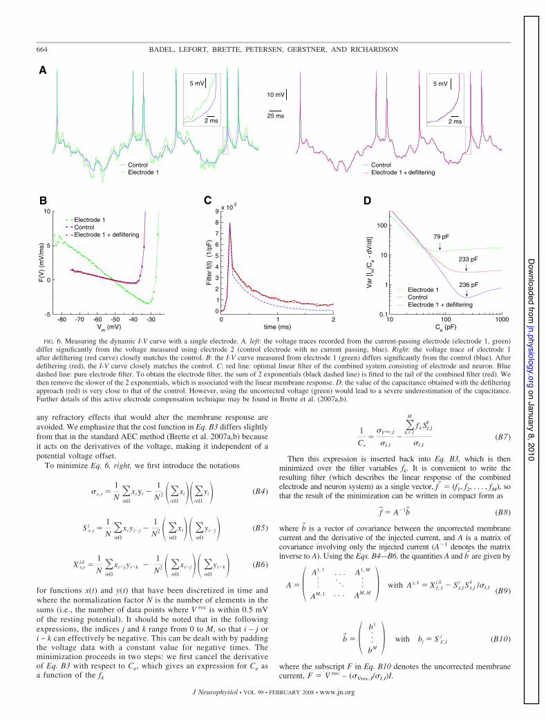
The faithful extraction of cell response properties requires accuratemeasurements of the membrane voltage. However, when injectingcurrent and monitoring voltage simultaneously from a single elec-trode, the filtering properties of the electrode may affect the measure-ments to a considerable extent. Although standard techniques areavailable to compensate electrode capacitance and access resistance,in the case of strong, high-frequency stimuli, this correction is notsufficient (Fig. 6), and some additional compensation is required.

Recently an active electrode compensation (AEC) technique wasintroduced (Brette et al. 2005, 2007a,b) that solves this problem,allowing for the simultaneous injection of current and measurement ofvoltage using a single electrode. To verify this compensation tech-nique for the dynamic I-V curve protocol, we performed recordings indouble-patch configuration with one electrode (referred to as electrode1) simultaneously injecting current and recording voltage, while theother electrode (control electrode 2) was used only to monitor thevoltage. In general, the uncompensated voltage measured from elec-trode 1 showed a significant deviation from the control (Fig. 6).Following the AEC methodology, we will now explain how theseartifacts can be removed from the voltage trace of electrode 1 throughthe estimation of the electrode filter without knowledge of the voltagefrom the control electrode, so as to allow for the measurement ofdynamic I-V curves from single-electrode recordings.

Electrode filter

We assume that the voltage across the electrode is a linearly filteredversion of the input current I(t). The recorded voltage V rec is the sumof the true membrane voltage V and the electrode voltage V el, thelatter of which we write as a convolution integral of the current withthe (unknown) electrode filter f(s)

V rec +t, $ V +t, & V el +t, $ V +t, &)0

4

f+s, I +t % s,ds (B1)

On the other hand, for a linear membrane the voltage can alsobe written in terms of a filter g(s) such that V(t) ! V0 % 50

4g(s)

I(t – s)ds. Therefore we cannot expect to determine the electrodefilter directly but rather the combined filter f(s) ! f(s) % g(s) of thesystem consisting of the electrode and the neuron. It is this filter thatwill be determined in the next section.

Optimization procedure

We have seen in the main text that the membrane capacitance canbe estimated from a variance minimization procedure. In our single-electrode approach, the variance must be calculated using the true,corrected membrane voltage, V(t) ! V rec(t) & 50

4f(s)I(t – s)ds. In

analogy with Eq. 6, left, of the main text, we therefore minimize thefunction

E $ var% I

Ce% V rec &)

0

4

f +s, I +t % s,ds&V

(B2)

with respect to both the filter f(s) and the capacitance Ce, where the dotdenotes the time derivative. Practically, the discrete form of thisequation is used

E $ var * Ii

Ce% V i

rec & +k!0

M

fk Ii&k,i*$

(B3)

Here, V irec and Ii are the uncompensated voltage and current data at

time step i, and the derivatives are calculated as forward differences,V i

rec ! (V i%1rec – Vi

rec)/'t, and Ii ! (Ii%1 – Ii)/'t, where 't denotes thetime step of the recording (1/'t ! + is the sampling frequency inkHz). fk is the kth value of the filter and represents how much of therecorded voltage at a given time is due to the current that was injectedk time steps earlier. M is the total number of points in the filter (a wayto efficiently choose this parameter is discussed in the following text).The subscript i ! $ indicates that the variance is calculated over theset $ of those data points that are both (i) close to the resting potential((V rec – Vrest( #0.5 mV), so that we can expect the membrane tobehave linearly, and (ii) lie . 200 ms after the peak of a spike, so that




Dow

nloaded from


any refractory effects that would alter the membrane response areavoided. We emphasize that the cost function in Eq. B3 differs slightlyfrom that in the standard AEC method (Brette et al. 2007a,b) becauseit acts on the derivatives of the voltage, making it independent of apotential voltage offset.

To minimize Eq. 6, right, we first introduce the notations

#x,y $1

N+i*$

xi yi %1

N 2 #+i*$

xi$#+i*$

yi$ (B4)

S x,yj $

1

N+i*$

xi yi&j %1

N2 # +i*$

xi$# +i*$

yi&j$ (B5)

X x,yj,k $

1

N+i*$

xi&j yi&k %1

N2 # +i*$

xi&j$# +i*$

yi&k$ (B6)

for functions x(t) and y(t) that have been discretized in time andwhere the normalization factor N is the number of elements in thesums (i.e., the number of data points where V rec is within 0.5 mVof the resting potential). It should be noted that in the followingexpressions, the indices j and k range from 0 to M, so that i – j ori – k can effectively be negative. This can be dealt with by paddingthe voltage data with a constant value for negative times. Theminimization proceeds in two steps: we first cancel the derivativeof Eq. B3 with respect to Ce, which gives an expression for Ce asa function of the fk

1

Ce

$#V rec,I

#I,I%+k!1

M

f k SI, Ik

#I,I(B7)

Then this expression is inserted back into Eq. B3, which is thenminimized over the filter variables fk. It is convenient to write theresulting filter (which describes the linear response of the combinedelectrode and neuron system) as a single vector, f! ! (f1, f2, . . . , fM), sothat the result of the minimization can be written in compact form as

f! $ A&1b! (B8)

where b! is a vector of covariance between the uncorrected membranecurrent and the derivative of the injected current, and A is a matrix ofcovariance involving only the injected current (A&1 denotes the matrixinverse to A). Using the Eqs. B4—B6, the quantities A and b! are given by

A $ - A1, 1 . . . A1, M

···· · ·

···AM, 1 · · · AM, M . with A j, k $ X I, I

j,k % S I, Ij S I, I

k /#I,I (B9)

b! $ - b1

···bM . with bj $ S F, I

j (B10)

where the subscript F in Eq. B10 denotes the uncorrected membranecurrent, F ! V rec – (#Vrec,I/#I,I)I.

ControlElectrode 1

ControlElectrode 1 + defiltering

10 100 1000Ce (pF)

0.1

1

10

100

Var

[Iin/C

e - d

V/d

t]

233 pF

Electrode 1ControlElectrode 1 + defiltering

-80 -70 -60 -50 -40 -30Vm (mV)

-5

0

5

10

F(V

) (m

V/m

s)

Electrode 1 Control Electrode 1 + defiltering

0 1 2time (ms)

0

1

2

3

4

5

6

7

8

9F

ilter

f(t)

(1/

pF)

x 10-2

79 pF

236 pF

A

25 ms

B D

10 mV

5 mV

2 ms

5 mV

2 ms

C

FIG. 6. Measuring the dynamic I-V curve with a single electrode. A, left: the voltage traces recorded from the current-passing electrode (electrode 1, green)differ significantly from the voltage measured using electrode 2 (control electrode with no current passing, blue). Right: the voltage trace of electrode 1after defiltering (red curve) closely matches the control. B: the I-V curve measured from electrode 1 (green) differs significantly from the control (blue). Afterdefiltering (red), the I-V curve closely matches the control. C: red line: optimal linear filter of the combined system consisting of electrode and neuron. Bluedashed line: pure electrode filter. To obtain the electrode filter, the sum of 2 exponentials (black dashed line) is fitted to the tail of the combined filter (red). Wethen remove the slower of the 2 exponentials, which is associated with the linear membrane response. D: the value of the capacitance obtained with the defilteringapproach (red) is very close to that of the control. However, using the uncorrected voltage (green) would lead to a severe underestimation of the capacitance.Further details of this active electrode compensation technique may be found in Brette et al. (2007a,b).




Dow

nloaded from


In practice, the value of the cost function (Eq. B3) at the minimumdiminishes with increasing filter length M but increases again for largeM due to numerical errors; thus there is an optimal value for M thatcan be found by standard optimization methods. We observed that ingeneral, a value of M such that the total length of the filter isapproximately one membrane time constant (10–20 ms) provides agood choice.

Correction for the membrane filtering

The optimal filter derived in the previous section contains a slowcomponent that is due to the membrane filtering. This componentmust be identified and removed from the overall filter to obtain thecorrect electrode filter. As can be seen in Fig. 6, the filter comprisesa fast, high-amplitude rise and fall followed by a slow relaxation. Todecouple the component of the electrode from that of the membrane,the slow relaxation is fitted with the sum of two exponentials, one witha fast time constant (of the order of 0.2–0.5 ms) that is due to theelectrode, the other with a slower time constant (of the order of tensof milliseconds) that is due to the membrane. Then the slow expo-nential is subtracted from the combined filter to yield the electrodefilter (Fig. 6). Using this electrode filter, the component of the voltagedue to the electrode can be calculated and subtracted from the voltagetrace to obtain the correct membrane voltage (Fig. 6, right). The entiremethod described in the main text can then be applied to the correctedvoltage trace. Finally, it can be noted that a more sophisticatedelectrode compensation method can also be used (Brette et al.2007a,b) based on a deconvolution procedure.

G R A N T S

C.C.H. Petersen, W. Gerstner, and L. Badel acknowledge support from theSwiss National Science foundation. R. Brette acknowledges support from aFrench Agence Nationale de la Recherche grant (HR-CORTEX). M.J.E.Richardson was partially supported by a European grant Fast Analog Com-puting with Emergent Transient States during his stay in Lausanne andcurrently holds a Research Councils United Kingdom Academic Fellowship.

D I S C L O S U R E

The authors state that there are no conflicts of interest.

R E F E R E N C E S

Abbott LF, van Vreeswijk C. Asynchronous states in a network of pulse-coupled oscillators. Phys Rev E 48: 1483–1490, 1993.

Brette R, Gerstner W. Adaptive exponential integrate-and-fire model as aneffective description of neuronal activity. J Neurophysiol 94: 3637–3642,2005.

Brette R, Piwkowska Z, Rudolph M, Bal T, Destexhe A. A non-parametricelectrode model for intracellular recording. Neurocomputing 70: 1597–1601, 2007a.

Brette R, Piwkowska Z, Rudolph-Lilith M, Bal T, Destexhe A. High-resolution intracellular recordings using a real-time computational model ofthe electrode. http://arxiv.org/abs/0711.2075, 2007b.

Brette R, Rudolph M, Piwkowska Z, Bal T, Destexhe A. How to emulatedouble-electrode recordings with a single-electrode? A new method ofactive electrode compensation. Soc Neurosci Abstr 31: 688.2, 2005.

Brunel N, Hakim V. Fast global oscillations in networks of integrate-and-fireneurons with low firing rates. Neural Comput 11: 1621–1671, 1999.

Brunel N, Hakim V, Richardson MJE. Firing-rate resonance in a generalizedintegrate-and-fire neuron with subthreshold resonance. Phys Rev E 67:051916, 2003.

Burkitt AN. Balanced neurons: analysis of leaky integrate-and-fire neuronswith reversal potentials. Biol Cybern 85: 247–255, 2001.

Burkitt AN. A review of the integrate-and-fire neuron model. I. homogeneoussynaptic input. Biol Cybern 95: 1–19, 2006.

Chacron MJ, Lindner B, Longtin A. Threshold fatigue and informationtransfer. J Comput Neurosci 23: 301–311, 2007.

Clopath C, Jolivet R, Rauch A, Luscher HR, Gerstner W. Predictingneuronal activity with simple models of the threshold type: adaptive expo-nential integrate-and-fire model with two compartments. Neurocomput 70:1668–1673, 2007.

Destexhe A, Rudolph M. Extracting information from the power spectrum ofsynaptic noise. J Comput Neurosci 17: 327–345, 2004.

Destexhe A, Rudolph M, Fellous JM, Sejnowski TJ. Fluctuating synapticconductances recreate in vivo-like activity in neocortical neurons. Neuro-science 107: 13–24, 2001.

Ermentrout GB. Type I membranes, phase resetting curves, and synchrony.Neural Comput 8: 979–1001, 1996.

Ermentrout GB, Kopell N. Parabolic bursting in an excitable system coupledwith a slow oscillation. SIAM J Appl Math 46: 233–253, 1986.

Fourcaud-Trocme N, Brunel N. Dynamics of the instantaneous firing rate inresponse to changes in input statistics. J Comput Neurosci 18: 311–321,2005.

Fourcaud-Trocme N, Hansel D, van Vreeswijk C, Brunel N. How spikegeneration mechanisms determine the neuronal response to fluctuatinginputs. J Neurosci 23: 11628–11640, 2003.

Fuortes MGF, Mantegazzini F. Interpretation of the repetitive firing of nervecells. J Gen Physiol 45: 1163–1179, 1962.

Geisler C, Goldberg J. A stochastic model of the repetitive activity ofneurons. Biophys J 6: 53–69, 1966.

Gerstner W. Population dynamics of spiking neurons: fast transients, asyn-chronous states and locking. Neural Comput. 12: 43–89, 2000.

Gerstner W, Kistler WM. Spiking Neuron Models. Cambridge, UK: Cam-bridge, 2002.

Gerstner W, van Hemmen JL. Coherence and incoherence in a globallycoupled ensemble of pulse-emitting units. Phys Rev Lett 71: 312–315,1993.

Gigante G, Mattia M, Del Giudice P. Diverse population-bursting modes ofadapting spiking neurons. Phys Rev Lett 98: 148101, 2007.

Gutkin BS, Ermentrout GB. Dynamics of membrane excitability deter-mine inter-spike interval variability: a link between spike generationmechanisms and cortical spike train statistics. Neural Comput 10: 1047–1065, 1998.

Hodgkin AL, Huxley AF. A quantitative description of membrane current andits application to conduction and excitation in nerve. J Physiol 117: 500–544, 1952.

Hodgkin AL, Huxley AF, Katz B. Measurement of current-voltage relationsin the membrane of the giant axon of Loligo. J Physiol 116: 424–448, 1952.

Huys QJM, Ahrens MB, Paninski L. Efficient estimation of detailed single-neuron models. J Neurophysiol 96: 872–890, 2006.

Izhikevich EM. Which model to use for cortical spiking neurons? IEEE Trans.Neural Networks 15: 1063–1070, 2004.

Jolivet R, Lewis TJ, Gerstner W. Generalized integrate-and-fire models ofneuronal activity approximate spike trains of a detailed model to a highdegree of accuracy. J Neurophysiol 92: 959–976, 2004.

Jolivet A, Rauch A, Luscher H-R, Gerstner W. Predicting spike timing ofneocortical pyramidal neurons by simple threshold models. J ComputNeurosci 21: 35–49, 2006.

Kistler WM, Gerstner W, van Hemmen JL. Reduction of Hodgkin-Huxleyequations to a single-variable threshold model. Neural Comput 9: 1015–1045, 1997.

Koch C. Biophysics of Computation. New York: Oxford, 1999.Lapicque L. Recherches quantitatives sur l’excitation electrique des nerfs

traitee comme une polarisation. J Physiol Pathol Gen 9: 620 – 635,1907.

Latham PE, Richmond BJ, Nelson PG, Nirenberg S. Intrinsic dynamics inneuronal networks. I. Theory. J Neurophysiol 83: 808–827, 2000.

Lindner B, Garcıa-Ojalvo J, Neiman A, Schimansky-Geier L. Effects ofnoise in excitable systems. Phys Reports 392: 321–424, 2004.

Lindner B, Longtin A. Effect of an exponentially decaying threshold on thefiring statistics of a stochastic integrate-and-fire neuron. J Theor Biol 232:505–521, 2005.

McCormick DA, Shu Y, Yu Y. Neurophysiology: Hodgkin and Huxleymodel—still standing? Nature 445: E1–E2, 2007.

Naundorf B, Wolf F, Volgushev M. Unique features of action potentialinitiation in cortical neurons. Nature 440: 1060–1063, 2006.

Paninski L, Pillow JW, Simoncelli EP. Maximum likelihood estimation of astochastic integrate-and-fire neural encoding model. Neural Comput 16:2533–2561, 2004.

Rauch A, La Camera G, Luscher HR, Senn W, Fusi S. Neocorticalpyramidal cells respond as integrate-and-fire neurons to in vivo-like inputcurrents. J Neurophysiol 90: 1598–1612, 2003.

Richardson MJE. Effects of synaptic conductance on the voltage distributionand firing rate of spiking neurons. Phys Rev E 69: 051918, 2004.




Dow

nloaded from


Richardson MJE, Brunel N, Hakim V. From subthreshold to firing-rateresonance. J Neurophysiol 89: 2538–2554, 2003.

Richardson MJE, Gerstner W. Synaptic shot noise and conductance fluctu-ations affect the membrane voltage with equal significance. Neural Comput17: 923–947, 2005.

Stein RB. The information capacity of nerve cells using a frequency code.Biophys J 7: 797–826, 1967.

Swensen AM, Marder E. Multiple peptides converge to activate the same

voltage-dependent current in a central pattern-generating circuit. J Neurosci20: 6752–6759, 2000.

Uhlenbeck GE, Ornstein LS. On the theory of the brownian motion. Phys Rev36: 823–841, 1930.

Wang XJ, Buzsaki G. Gamma oscillation by synaptic inhibition in a hip-pocampal interneuronal network model. J Neurosci 16: 6402–6413, 1996.

Wiener N. Nonlinear Problems in Random Theory. Cambridge, MA: MITPress, 1958.




Dow

nloaded from


Documents

Dynamic Curves Are Reliable Predictors of Naturalistic