Embed Size (px)
Citation preview

This is the author manuscript accepted for publication and has undergone full peer review but has
not been through the copyediting, typesetting, pagination and proofreading process, which may
lead to differences between this version and the Version of Record. Please cite this article as doi:
10.1111/poms.12559
This article is protected by copyright. All rights reserved
Auth
or
Manuscript
Submitted to Production and Operations Management
manuscript (1)
Dynamic Customer Acquisition and RetentionManagement
(Authors’ names blinded for peer review)
In consulting, finance, and other service industries, customers represent a revenue stream, and must be
acquired and retained over time. In this paper, we study the resource allocation problem of a profit max-
imizing service firm that dynamically allocates its resources towards acquiring new clients and retaining
unsatisfied existing ones. The interaction between acquisition and retention in our model is reflected in the
cash constraint on total expected spending on acquisition and retention in each period. We formulate this
problem as a dynamic program in which the firm makes decisions in both acquisition and retention after
observing the current size of its customer base and receiving information about customers in danger of
attrition, and we characterize the structure of the optimal acquisition and retention strategy.
We show that when the firm’s customer base size is relatively low, the firm should spend heavily on
acquisition and try to retain every unhappy customer. However, as its customer base grows, the firm should
gradually shift its emphasis from acquisition to retention, and it should also aim to strike a balance between
acquisition and retention while spending its available resources. Finally, when the customer base is large
enough, it may be optimal for the firm to begin spending less in both acquisition and retention. We also
extend our analysis to situations where acquisition or retention success as a function of resources allocated is
uncertain and show that the optimal acquisition and retention policy can be surprisingly complex. However,
we develop an effective heuristic for that case. This paper aims to provide service managers some analytics
principles and effective guidelines on resource allocation between these two significant activities based on
their firm’s customer base size.
Key words : Dynamic Programming, Service Operations, OM-Marketing Interface
1. Introduction
Customer retention is a growing concern for firms in many industries. From consulting, to
finance, to cable service, customer retention is the key to long term profitability for many
companies. Also critical is a firm’s ability to acquire new customers in order to build its
customer base. These two considerations in parallel naturally lead to the question of how
a service firm should manage the trade-off between customer acquisition and retention.
Customer acquisition and retention are costly activities for a firm, and the firm may be
prone to fail at this process due to a lack of guidance or actionable strategies. For example,
1Thisarticleisprotectedbycopyright.Allrightsreserved
Auth
or
Manuscript

Authors’ names blinded for peer review
2 Article submitted to Production and Operations Management; manuscript no. (1)
during the dot-com boom of the late 1990s and early 2000s many companies spent millions
on customer acquisition without proper processes in place for retention.
This paper is derived from industry experience of the first author, who faced this problem
while working at a small third-party-financing company. The firm lent money to patients
for medical procedures through a network of doctors. Thus, these doctors were considered
as the firm’s customers because their satisfaction and service usage drove profitability for
the firm. A sales force located throughout the United States was tasked with acquiring
new customers as well as visiting existing ones to keep them satisfied with the service
being provided. The trade-off between acquisition and retention was widely discussed at
the company, and its impact on profitability was significant. During this period, the firm
heavily emphasized acquisition while experiencing rapid growth. Analysis supported this
practice, concluding that time and money were better spent in acquisition. However, as the
firm matured, two things happened. First, the efforts in acquisition became futile, because
incremental prospects were harder to acquire and less profitable. Second, attrition became
a problem because the firm had neglected some of the existing users. Naturally the focus
started to shift towards retention, though subsequent analyses indicated that the shift
occurred too late. A primary motivating factor for this research is to build a model that
helps companies better allocate resources towards acquisition and retention over time.
We consider the acquisition and retention trade-off from the perspective of a service
manager. The key research questions relate to the timing and quantity of spend in each
of these two areas: How many customers should be targeted and how can the manager
appropriately determine the effort that should be spent on acquisition of new accounts
versus development of existing accounts? Does the strategy change as the customer base of
the firm grows over time? Is there an efficient number of customers for the firm to maintain
over time?
Acquisition and retention management is an issue of alignment between marketing and
operations, and thus deserves consideration in the operations management and service
Thisarticleisprotectedbycopyright.Allrightsreserved
Auth
or
Manuscript

Authors’ names blinded for peer review
Article submitted to Production and Operations Management; manuscript no. (1) 3
operations literature. While the specific acquisition and retention tactics themselves may
be marketing (or sales) activities, they need to be balanced against operations and ser-
vice capabilities. The service capabilities affect the ability of the firm to allocate resources
towards acquisition and retention. Therefore, acquisition and retention activities should be
carefully coordinated between marketing and operations. Furthermore, we make the dis-
tinction between specific acquisition and retention strategies and the higher level resource
allocation decision about how much capital or effort to spend in these areas. The latter is
often an operational decision of a firm.
We study how a service operations manager should dynamically allocate his resources
towards acquisition/retention when faced with limited resources (e.g., a limited budget to
spend on these activities). We characterize how the acquisition/retention policy dynami-
cally depends on the number of customers of the firm, the number of ‘unhappy’ customers
in danger of canceling service, and the firm’s total budget (cash constraint) for acquisition
and retention. Our results indicate that early on when the firm has few customers, the firm
should spend heavily on acquisition and try to retain every ‘unhappy’ customer. However,
as the customer base of the firm grows, the firm may reach a point where it is not optimal
to retain all unhappy customers due to resource constraint on acquisition and retention
activities. In this situation the firm needs to carefully strike a balance between acquisition
and retention while using up all of the available budget. Finally, when the customer base is
large enough, it may be optimal for the firm to begin spending less in both acquisition and
retention. This result, i.e., the firm may reach a point in the number of customers it wants
to have and curtails its acquisition and retention activities beyond this critical size, may
seem unintuitive at first. However, it is driven by the fact that the marginal acquisition
and retention costs are increasing in the number of customers acquired and retained, while
the marginal increase in revenues is decreasing in the number of customers the firm serves.
These are reasonable assumptions since sales forces acquire and retain the easiest prospects
in a market first and acquiring and retaining customers gets more costly as the number of
Thisarticleisprotectedbycopyright.Allrightsreserved
Auth
or
Manuscript

Authors’ names blinded for peer review
4 Article submitted to Production and Operations Management; manuscript no. (1)
customers of the firm increases. For example, a few years ago telecommunication companies
such as Sprint decided to ‘hang up’ their high-maintenance customers, which corresponds
to refusing to retain customers beyond a certain point in our model.1 Another implication
of our results is that if the firm can become more efficient in acquisition and retention (by
reducing acquisition or retention costs, or finding ways to make its service more valuable
to customers so that customers are willing to pay more for service), it will enable the firm
to increase its efficient size, which then leads to an increased overall customer base.
As the economy has become more service oriented, the importance of maintaining cus-
tomer relationships is more critical today than ever before. The goal of this work is to
provide structural insights and analysis of the essential trade-offs that occur in managing
service industries, through the use of a dynamic decision making model. We begin with a
literature review in §2, present the model and results in §3, discuss a model extension with
heuristic in §4, before we conclude in §5. Throughout the paper we use the terms increas-
ing and decreasing to mean non-decreasing and non-increasing, respectively. Finally, all
mathematical proofs are given in the Appendix.
2. Literature Review
The trade-off between acquisition and retention has been primarily studied in the marketing
literature. The novel approach of our work is that we analyze this problem as a dynamic
one, which captures the dynamic nature of resource allocation over time. The vast majority
of other work is not dynamic. As a result, our approach has system dynamics in the form
of state transitions. We also use the machinery of stochastic optimization, in contrast to
most papers which use regression, empirical, or deterministic techniques.
In a well known article in Harvard Business Review, Blattberg and Deighton (1996)
establish the ‘customer equity test’ for determining the allocation of resources between
acquisition and retention of customers. Using a deterministic model, the main contribution
1 http://www.foxnews.com/story/2007/07/09/sprint-hangs-up-on-high-maintenance-customers/. Accessed May 2,2015.
Thisarticleisprotectedbycopyright.Allrightsreserved
Auth
or
Manuscript

Authors’ names blinded for peer review
Article submitted to Production and Operations Management; manuscript no. (1) 5
of this work is a simple calculation used to compare acquisition and retention costs with
potential benefits.
The marketing literature contains numerous sources analyzing the acquisition and reten-
tion trade-off. Reinartz et al. (2005) discuss the problem from a strict profitability per-
spective using industry data. They find that under-investment in either area can be detri-
mental to success while over-investment is less costly, and that firms often under-invest in
retention. Thomas (2001) discusses a statistical methodology for linking acquisition and
retention. Homburg et al. (2009) use a portfolio management approach to maintaining a
customer base.
Fruchter and Zhang (2004) is most closely related to our work in that it takes a dynamic
approach to analyze the trade-off between acquisition and retention. However, there are
fundamental differences between our approach and theirs. In Fruchter and Zhang (2004),
there are two firms and a fixed market in which customers use one firm or the other.
Acquisition represents converting customers from the other firm while retention is pre-
venting existing customers from switching to a competitor. Furthermore, their model is
a differential game in which they make very specific assumptions on how effective acqui-
sition and retention are at generating sales, namely that effectiveness is proportional to
the square root of the expenditure. With this special model structure, Fruchter and Zhang
(2004) show that equilibrium retention increases in a firm’s market share while equilibrium
acquisition decreases. Our work does not assume a fixed market, or specific functions that
determine the relationship between expenditure and impact, and our work also captures
randomness (Fruchter and Zhang (2004) is deterministic). Due to the fact that we do not
assume a fixed market where the only way to obtain more customers is to convert them
from another company, our insights are also different than Fruchter and Zhang (2004).
A recent paper on customer acquisition and retention from the operations management
literature is Dong et al. (2011), and the reader is referred to their introduction for addi-
tional references on the problem studied. Dong et al. (2011) consider joint acquisition
Thisarticleisprotectedbycopyright.Allrightsreserved
Auth
or
Manuscript

Authors’ names blinded for peer review
6 Article submitted to Production and Operations Management; manuscript no. (1)
and retention, and use an incentive mechanism design approach to solve their problem.
Additionally, they consider the question of direct versus indirect selling, in which the firm
decides whether to use a sales force (for which an incentive is designed) or not. Their
problem is static, where decisions are made only once.
Sales force management is a topic well-studied from the incentive-design perspective by
others in addition to Dong et al. (2011). It often represents a traditional adverse selection
problem where designing a proper incentive structure can be difficult and costly due to the
economics concept of information rent that must be paid to the sales agent to induce them
to truthfully reveal their hidden information. Papers that discuss sales incentives in this
context come from both the economics and operations management literature. From the
economics literature, important works include Gonik (1978), Grossman and Hart (1983),
Holmstrom (1979), and Shavell (1979). These papers set the stage for how moral hazard
applies in the sales context and propose potential incentive mechanisms. In the operations
literature, sales force incentives have been discussed primarily in the context of inventory-
control, and manufacturing. Important references include Chen (2005), Porteus and Whang
(1991), and Raju and Srinivasan (1996). These papers do not discuss the trade-off between
acquisition and retention.
There also exists a body of literature on customer management from a service and
capacity perspective. Hall and Porteus (2000) study a dynamic game model of capacity
investment where maintaining sufficient capacity relative to market share drives retention,
and excess capacity leads to acquisition. With a special structure for costs and benefits
of capacity, they are able to solve explicitly for the subgame perfect equilibrium. Related
dynamic game inventory-based competition research includes Ahn and Olsen (2011) and
Olsen and Parker (2008). In these papers, retention and acquisition are driven by fill rates,
and are not explicit decisions, as in our paper.
There is a broad literature on service failure recovery, which generally finds that it is
beneficial to recover dissatisfied customers after a service failure, see for example, Spreng
Thisarticleisprotectedbycopyright.Allrightsreserved
Auth
or
Manuscript
Authors’ names blinded for peer review
Article submitted to Production and Operations Management; manuscript no. (1) 7
et al. (1995). This literature also discusses the ‘service recovery paradox’, which says that
previously dissatisfied customers respond most strongly to recovery efforts (see Matos
et al. (2007)). Our concept of ‘retention’ is more pro-active, and we do not explicitly
model service failures, but instead assume that some customers are ‘unhappy’ , and we
have the option to work on retaining them once we find out their unhappiness. (Our
model is especially relevant in many settings such as cable or telecommunications where
a set of customers express unhappiness with the service absent a specific explicit service
failure which caused the unhappiness). Another related area of literature is organizational
learning, where acquisition and retention are framed as exploration and exploitation (as it
pertains to new innovations/technologies). A seminal paper in this area is March (1991)
and a more recent update is Gupta et al. (2006). The general finding in these papers is
that exploitation is beneficial in the short term but can have negative consequences in the
long term unless accompanied by exploration. Thus the key to success for a firm is to be
ambidextrous across both capabilities of exploration and exploitation.
The main contribution of this paper is to study the acquisition and retention manage-
ment problem using a dynamic optimization approach. With this approach, we are able to
incorporate the dynamic nature of this important resource allocation problem, and derive
managerial insights on optimal acquisition and retention related to the system dynam-
ics, e.g., how does a firm’s current level of satisfied and dissatisfied customers impact its
allocation decisions in acquisition and retention?
We believe it is important to study dynamic acquisition and retention for a firm due to
the following reasons. First of all, we argue that a dynamic model cannot be reduced to a
single period model as one needs at least two periods for the investment in acquisition and
retention to later pay-off. Second, it is the dynamic nature of our model that makes it more
representative of reality and more general, and enables us to obtain a richer characterization
of optimal acquisition and retention policies’ dependence on the size of the customer base,
the size of the ‘unhappy’ customers, as well as the available budget for acqusition/retention.
Thisarticleisprotectedbycopyright.Allrightsreserved
Auth
or
Manuscript

Authors’ names blinded for peer review
8 Article submitted to Production and Operations Management; manuscript no. (1)
3. Model and Main Results
We model the acquisition and retention resource allocation problem as an N period finite-
horizon dynamic program. The decision period is indexed by n, n= 1, . . . ,N . At the begin-
ning of period n, the firm knows its number of customers, xn, and a random fraction ρn
of its customers are identified as being at high risk for attrition. For simplicity we call
these customers ‘unhappy’ customers. After observing the number of ‘unhappy’ customers,
the firm decides how many customers to retain, and how many new customers to acquire,
decisions we denote by Rn and An respectively. Note that ρ1, . . . , ρN are random variables
and ρn is realized (and observed) at the beginning of period n. As an example of how this
works in practice, it is common in the cable industry for customers to call and ask to dis-
connect service, or otherwise express discontent. Once these customers are identified, the
cable company will make a retention offer with enhanced service or lower pricing. During
the same period n, the firm also signs up new acquisition prospects.
In this section we consider the situation in which a firm decides how many of its ‘unhappy’
customers to retain and how many new customers to acquire, and the firm will spend the
necessary resources to implement the decision in the period. Therefore, the outcomes for
these decisions are deterministic, An (acquisition) and Rn (retention) respectively, while
the costs to implement the decisions are random, with average values denoted by CAn (An)
and CRn (Rn), respectively. To make the trade-off between acquisition and retention explicit,
we have a cash constraint on total expected spending in each period of our model. This
constraint is given as CAn (An) +CR
n (Rn) ≤ Sn for a positive number Sn. Because of such
a constraint, our problem is a service capacity one in the traditional sense. Note that
because our acquisition and retention costs are random, the cash constraint applies to
expected acquisition and retention costs. This is reasonable because when firms are faced
with uncertain costs, they are likely to budget a priori based on expected outcomes.
Because customers represent a revenue stream for the firm, the expected revenue gener-
ated during period n, given that the number of customers at the beginning of period n is
Thisarticleisprotectedbycopyright.Allrightsreserved
Auth
or
Manuscript
Authors’ names blinded for peer review
Article submitted to Production and Operations Management; manuscript no. (1) 9
xn, is denoted by Mn(xn). Note that Mn(xn) represents the customer revenue minus any
variable costs associated with providing service to the customer base of size xn.
It is also possible for some ‘happy’ customers to discontinue service even though the
firm has no prior indication of their dissatisfaction with the service. We denote the random
percentage of ‘happy’ customers that continue service in period n as γn ∈ [0,1] (thus, 1−γn
is the fraction of ‘happy’ customers that discontinue service). At the beginning of the next
period, n+1, the number of customers evolves according to state transition
xn+1 = γn(1− ρn) xn +Rn +An, n= 1,2, . . . ,N − 1. (1)
Thus, the firm retains γn of the‘happy’ customers and Rn of the ‘unhappy’ ones, while
adding An in acquisition. In this section we assume Rn and An are deterministic, and we
will study the case of uncertain acquisition and uncertain retention in the next section.
Suppose the decision maker uses a discount factor, α∈ (0,1), in computing its profit. The
objective of the firm is to balance acquisition and retention in each period to maximize its
total expected discounted profits. Let Vn(xn) be the maximum expected total discounted
profit from period n until the end of the planning horizon, given that the number of
customers at the beginning of period n is xn. Then the optimality equation is
Vn(xn) = Mn(xn)+Eρn
[
max0≤An,0≤Rn≤ρnxn,CA
n (An)+CRn (Rn)≤Sn
(
−CAn (An)−CR
n (Rn) (2)
+αEγn [Vn+1
(
γn(1− ρn) xn +Rn +An
)
])]
.
The boundary condition is VN+1(x)≡ 0 for all x≥ 0, implying that the firm makes profits
only through period N .
The optimality equation is described as follows. Suppose xn is the number of customers at
the beginning of period n. The firm earns a revenue related to the size of its customer base
in period n, given by Mn(xn). After observing the number of ‘unhappy’ customers, ρnxn,
the firm decides how many ‘unhappy’ customers to retain and how many new customers
to acquire, with respective costs CRn (Rn) and CA
n (An). The firm may spend up to Sn total
Thisarticleisprotectedbycopyright.Allrightsreserved
Auth
or
Manuscript

Authors’ names blinded for peer review
10 Article submitted to Production and Operations Management; manuscript no. (1)
on acquisition and retention. The state at the beginning of the next period is given by
equation (1). Since the proportion of ‘unhappy’ customers is random, we need to take
expectation with respect to ρn, and then with respect to γn. Because the firm’s decision is
made after realization of the number of ‘unhappy’ customers, the optimization decision is
inside the first expectation in (2).
Assumption 1. The cost functions for the retention of existing customers and acqui-
sition of new customers given by CRn (·) and CA
n (·) are increasing and strictly convex with
continuous derivatives defined on a domain of [0,∞).
More acquisition or retention is always more costly to the firm, thus CRn (·) and CA
n (·) are
increasing functions. Assumption 1 also assumes that retention and acquisition costs are
both convex in the number of targets captured by the firm in each category. This can be
explained as follows. When given targets, sales forces usually acquire or retain the easiest
prospects in a market first. As the best prospects are acquired, acquisition and retention
grows more difficult and costly. Furthermore, getting more work from a fixed-size sales
force could result in overtime and other costs, which also leads to an increasing convex
cost function.
Assumption 2. The expected revenue function Mn(xn) is increasing concave and con-
tinuous in xn with domain of [0,∞).
The expected revenue is clearly increasing in the number of customers using the firm’s
service. Here we also assume that it is concave in the number of customers. Larger and
higher margin customers are likely to be targeted first in acquisition, so incremental cus-
tomers will generate less revenue. In the third-party-financing industry, incremental cus-
tomers tend to be less profitable because they are likely to be smaller and more skeptical
of the benefit associated with the service being provided. In addition, as the prospects
valuing the service most are acquired, it takes more effort and better terms to successfully
acquire more skeptical customers.
Thisarticleisprotectedbycopyright.Allrightsreserved
Auth
or
Manuscript
Authors’ names blinded for peer review
Article submitted to Production and Operations Management; manuscript no. (1) 11
Our model complements the landmark work of Blattberg and Deighton (1996) that
establishes the ‘customer equity test’. In their model, as in ours, acquisition and retention
success is a concave function of total spending, customers generate a per-period revenue,
and a firm makes acquisition and retention decisions. However, the primary difference is
that they assume that acquisition and retention decisions are made only once, and then
maintained over the lifetime of a customer. In our model, the firm can dynamically adjust
its strategy over time, which enables us to characterize these dynamic decisions as a func-
tion of the size of the firm’s customer base and the number of its ‘unhappy’ customers. Also,
we allow costs and revenues to have a more general form, while Blattberg and Deighton
(1996) assume linear revenues and an exponential spending/outcome relationship. Finally,
we have a cash constraint on total expected acquisition and retention activities, as dis-
cussed.
Before proceeding to the main result, we present here a preliminary modularity result
which will be useful in our characterization of the firm’s optimal strategy.
Lemma 1. Given continuous and strictly concave functions f(·), g(·) and h(·), a non-
negative constant K, and a non-negative random variable ǫ, the optimal solution to the
optimization problem
maxx≥0,y≥0
f(x)+ g(y)+E[h(x+ y+ ǫK)],
denoted by x∗ and y∗, are decreasing in K with slopes between 0 and -1.
The result above states that as K varies, the optimal x∗ and y∗ move in the same direc-
tion as each other, and in the opposite direction as K. Note that this is a meaningful
result but it does not follow from modularity analysis in Topkis (1998). This is because,
the objective function for the optimization problem above is submodular in (x, y,K), but
the optimization is maximization. There is no general comparative statics results on max-
imizing submodular functions when the decisions are not single dimensional (in this case
the decision is two-dimensional).
Thisarticleisprotectedbycopyright.Allrightsreserved
Auth
or
Manuscript

Authors’ names blinded for peer review
12 Article submitted to Production and Operations Management; manuscript no. (1)
With our technical result in Lemma 1, we are ready to present the main result of this
paper. The following theorem states that there exists a ρn-dependent threshold Qn(ρn),
decreasing in ρn, such that when the number of customers at the beginning of period n
is less than this threshold, the firm targets every ‘unhappy’ customer, while the optimal
number of acquired new customers is decreasing in the current customer base, i.e., in this
range the firm gradually shifts emphasis from acquisition to retention as its customer base
grows. The existence of a second ρn-dependent thresholdKn
1−ρndefines a second region where
the firm maximizes allowable resources in acquisition and retention while maintaining flat
levels of acquisition and retention spending. Finally when the firm’s customer base is
larger than both thresholds, the firm begins to target fewer and fewer customers in both
acquisition and retention; in this range, both the optimal acquisition and optimal retention
are decreasing in the customer base xn with slope no less than −(1− ρn).
Theorem 1. Suppose xn is the number of customers at the beginning of period n, and
the proportion of ‘unhappy’ customers is ρn.
(i) The optimal strategy for period n is determined by a critical number Kn, a decreas-
ing function Qn(ρn), and decreasing curves RU∗n (·), AU∗
n (·), and AW∗n (·) of slopes no less
than -1, such that a) if xn ≤ Qn(ρn), then the firm retains all ‘unhappy’ customers and
sets (An,Rn) = (min{AW∗n (xn), Sn − CR
n (ρnxn)}, ρnxn); b) if xn ∈ (Qn(ρn),Kn
1−ρn), then the
firm uses maximum allowable resource Sn and sets (An,Rn) = (AU∗n (Kn),R
U∗n (Kn)) with
AU∗n (Kn)+RU∗
n (Kn) = Sn; and c) in all other cases (An,Rn) = (AU∗n (xn(1−ρn)),R
U∗n (xn(1−
ρn))).
(ii) There exist increasing functions QAn (ρn) and QR
n (ρn) such that when xn ≥QRn (ρn),
the firm does no retention, and when xn ≥QAn (ρn), the firm does no acquisition.
(iii) There exists a critical threshold function x∗n(ρn), decreasing in ρn, such that, under
the optimal acquisition and retention policies the expected market size of the firm goes up
in the next period if the current market size is less than this threshold, and goes down
otherwise, i.e.,
E[xn+1]−xn =
{
≤ 0, if xn ≥ x∗n(ρn);
≥ 0, if xn ≤ x∗n(ρn).
Thisarticleisprotectedbycopyright.Allrightsreserved
Auth
or
Manuscript
Authors’ names blinded for peer review
Article submitted to Production and Operations Management; manuscript no. (1) 13
Therefore, under the optimal strategy, the firm will lose customers (in expectation) when
above a critical point and add customers (in expectation) when below that same point.
The optimal strategy stated in Theorem 1 takes an intuitive form. For a relatively small
base of customers, the firm should retain each and every ‘unhappy’ customer. In this region,
acquisition is also critical. After this point, there may exist a second region where the
firm spends Sn on acquisition and retention, the maximum allowable resource, but not
necessarily able to retain every ‘unhappy’ customer. Finally, as the customer base of the
firm grows large enough, it spends less on acquisition and retention. We remark that the
second region in the optimal acquisition and retention strategy characterization, i.e., b) of
case i), could be an empty set.
From the results of this section, we learn that a firm should shift resources from acquisi-
tion to retention as its customer base grows. However, this is only true up to some critical
point. After that point, there may first exist a region in which acquisition and retention
are constant due to the firm’s cash constraint; and when the customer base grows large
enough, the optimal strategy for the firm will be to invest less in both acquisition and
retention. Note that our result indicates that retention effort is a function of a firm’s cus-
tomer size, an insight that is consistent with much of the marketing literature. However,
compared with the marketing literature (e.g. Fruchter and Zhang (2004)), our results are
consistent only in the first region, where the firm increases retention as its customer base
grows and decreases acquisition. However, when the firm is large enough, our results pre-
dict less spending in both acquisition and retention. With our explicit cash constraint on
total expected acquisition and retention spending, we also characterize a region in which
the constraint is tight so the total acquisition and retention are constant.
We also want to point out that the threshold function x∗n(·) in (iii) depends on the
period n and is not a constant. The existence of a threshold x∗n(ρn) may appear counter-
intuitive at first, but it is to be expected. This is because, the firm’s revenue function is
increasing concave while its acquisition and retention costs are increasing convex. When
Thisarticleisprotectedbycopyright.Allrightsreserved
Auth
or
Manuscript
Authors’ names blinded for peer review
14 Article submitted to Production and Operations Management; manuscript no. (1)
the firm’s customer base is large enough, the marginal increase in acquisition/retention
cost may overgrow the marginal increase in revenue. Note that the existence of a critical
threshold of customers for the firm to have for a specific period does not indicate that
the firm should not grow its number of customers over time. Nothing about our model
and result regarding the existence of the x∗n (for each period n) prohibits the possibility
of firms growing its number of customers over time. First, it may be the case that the x∗n
are high (possibly even infinite) relative to a reasonable customer base, in which case the
firm is always targeting growth. Second, the values of x∗n can increase across periods. We
demonstrate this second point with two simple examples below.
In the first example, suppose that the costs of acquisition and retention decrease over
time due to experience gained by sales individuals performing these tasks. Even with
constant customer revenue rate, we will see that x∗n are increasing. Let Mn(xn) = 10xn with
ρn = γn = 0.5, for n= 1, . . . ,5. The acquisition and retention costs for the first period are
CA1 (A1) = 10000( A1
1000)2 and CR
1 (R1) = 5000( A1
1000)2, and then subsequent costs in periods 2,
3, 4 and 5 are given by 90%, 80%, 70% and 60% of these values respectively. In this case,
the x∗n values are given by x∗
1 = 2200, x∗2 = 2480, x∗
3 = 2770, x∗4 = 3110 and x∗
4 = 3323 (note
that these values typically depend on ρn, but in this example ρn is constant).
The second example assumes instead that costs are constant but customers become
more profitable over time because the firm finds ways to extract additional value through
cost efficiencies or cross selling. In this example let ρn = γn = 0.5, CAn (An) = 10000( An
1000)2
and CRn (Rn) = 5000( An
1000)2 for n = 1, . . . ,5. Revenues increase between periods and are
given by 6x1, 6x2, 6x3, 8x4, and 10x5 respectively for the periods 1 through 5. With these
parameters, the x∗n values are given by x∗
1 = 1231, x∗2 = 1234, x∗
3 = 1722, x∗4 = 2100 and
x∗5 = 2000, only dropping in the final period of the model.
Thus, our results indicate that if firms want to keep growing its customer base, they
need to find ways to reduce their acquisition and retention costs over time or find ways to
make customers more valuable over time (by potentially selling them additional services
Thisarticleisprotectedbycopyright.Allrightsreserved
Auth
or
Manuscript

Authors’ names blinded for peer review
Article submitted to Production and Operations Management; manuscript no. (1) 15
Figure 1 Optimal Acquisition and Retention Strategies in terms of number of customers x1 with fixed ρ1 = 0.5,
when Qn(ρn)>Kn
1−ρn(N = 2, M2(x2) = 10 ln(1+ x2
2), S1 = 10, CA
1 (A1) = ( A1
100)1.2, γ = 1 with probability
1, and CR1 (R1) = ( R1
100)1.1)
that the customers may be willing to buy). To the extent that the firm is able to do that,
in Theorem 1, the expected number of customers that a firm will have in each period will
be higher in expectation than in the previous period.
The optimal strategy is demonstrated in Figures 1 and 2, in which we can observe the
strategy and how it changes as a function of the customer base, xn, for a fixed value
of ρn. The two graphs differ in that the smaller cash-constraint in Figure 2 implies that
Qn(ρn)<Kn
1−ρn, creating a region in which acquisition and retention are flat, because the
firm is spending at the maximal level of Sn.
To further characterize the optimal strategy, we need the following result. In this result,
we use (CAn )
′(0) and (CRn )
′(0) to denote the right derivative of the cost functions at zero.
Lemma 2. If (CAn )
′(0) ≤ (CRn )
′(0), then QAn (ρn) ≥ QR
n (ρn) for all ρn > 0; and if
(CAn )
′(0) ≥ (CRn )
′(0), then QAn (ρn) ≤ QR
n (ρn) for all ρn > 0. In particular, if (CAn )
′(0) =
(CRn )
′(0), then QAn (ρn) =QR
n (ρn) for all ρn > 0.
The implication of Lemma 2 is that the monotone switching curves QAn (ρn) and QR
n (ρn)
do not cross, and they are ordered. Thus, for example, when QAn (ρn)≥QR
n (ρn) is true, the
customer base size beyond which the firm does not do any acquisition is always higher than
Thisarticleisprotectedbycopyright.Allrightsreserved
Auth
or
Manuscript

Authors’ names blinded for peer review
16 Article submitted to Production and Operations Management; manuscript no. (1)
Figure 2 Optimal Acquisition and Retention Strategies in terms of number of customers x1 with fixed ρ1 = 0.5,
when Qn(ρn)<Kn
1−ρn(N = 2, M2(x2) = 10 ln(1+ x2
2), S1 = 4, CA
1 (A1) = ( A1
100)1.2, γ = 1 with probability
1, and CR1 (R1) = ( R1
100)1.1)
the customer base beyond which the firm does no retention. Lemma 2 allows us to analyze
the optimal strategies when both parameters xn and ρn vary. For the purposes of the dia-
grams, let us assume that (CAn )
′(0)< (CRn )
′((CRn )
−1(Sn)) and (CRn )
′(0)< (CAn )
′((CAn )
−1(Sn))
such that the firm does both acquisition and retention when the cash constraint is tight,
because the marginal cost of acquisition (retention) at zero is smaller than the marginal
cost of retention (acquisition) when the cash constraint is tight.
In the first case, i.e., QRn (ρn)≤QA
n (ρn), the optimal strategy is demonstrated in Figure 3
as a function of xn and ρn. When both xn and ρn are small (region I), the optimal strategy
is to retain everyone, and also spend in acquisition. When both become larger, the firm will
still spend on both acquisition and retention, but may not retain all ‘unhappy’ customers
(regions II and III). When xn is still relatively small with a larger ρn, the firm should spend
up to the cash-constraint maximum (region II); when xn is large with ρn relatively small,
the firm will invest in just acquisition (region IV). Finally, when the number of customers
is really large, then the firm will spend neither on retention nor acquisition (region V).
The second case, i.e., when QRn (ρn)≥QA
n (ρn), is depicted in Figure 4. As in the previous
case, when both xn and ρn are small (region I), the optimal strategy is to retain everyone,
and spend some in acquisition. However, now there is another region (region II), when xn
Thisarticleisprotectedbycopyright.Allrightsreserved
Auth
or
Manuscript

Authors’ names blinded for peer review
Article submitted to Production and Operations Management; manuscript no. (1) 17
Figure 3 Case I - Optimal Acquisition and Retention Strategies in terms of number of customers xn and per-
centage ‘unhappy’ ρn when QRn (ρn)≤QA
n (ρn) (Region I - Retain all ‘unhappy’ and do some acquisition,
Region II - Retention and Acquisition up to the cash constraint, Region III - Some retention, some
acquisition, Region IV - Only acquisition, Region V - No spending)
is larger, in which the firm may retain everyone, but not spend anything in acquisition.
The firm spends on both acquisition and retention for relatively large ρn and small xn
(regions III and IV); spending up to the cash constraint when xn is smaller and ρn larger
(region III). When xn is large with ρn relatively small, the firm will invest only in retention
(region V). Finally, the firm invests in neither acquisition nor retention when the number
of customers is really large (region VI).
Lemma 2 allows us to develop detailed guidelines to firms on how to allocate their
valuable resources towards acquisition and retention in different ranges of the size of their
customer base and the fraction of dissatisfied customers (see Figures 3 and 4), and these
results are much more detailed and intricate than provided in the previous literature.
Indeed, as shown in Figures 3 and 4, the results indicate that there may be as many as 6
different regions in which the firm adapts different strategies based on these parameters.
In practice, one may think that the firm would always dedicate some resource towards
retention. However, this is not true in general. In the following, we present a sufficient
condition under which this is true.
Corollary 1. If there exists a positive number κ> 0 such that limxn+1→∞M′
n+1(xn+1)≥
Thisarticleisprotectedbycopyright.Allrightsreserved
Auth
or
Manuscript

Authors’ names blinded for peer review
18 Article submitted to Production and Operations Management; manuscript no. (1)
Figure 4 Case II - Optimal Acquisition and Retention Strategies in terms of number of customers xn and per-
centage ‘unhappy’ ρn when QRn (ρn)≥QA
n (ρn) (Region I - Retain all ‘unhappy’ and do some acquisition,
Region II - Retain all ‘unhappy’ with no acquisition, Region III - Retention and Acquisition up to the
cash constraint, Region IV - Some retention, some acquisition, Region V - Only retention, Region VI
- No spending)
κ ≥ (CRn )′(0)α
, then QRn (ρn) = ∞ and the firm will always do some retention, as long as
ρnxn > 0 (there are ‘unhappy’ customers) and (CRn )
′(0)< (CAn )
′((CAn )
−1(Sn)) (maximal cash
constraint spending involves some retention).
Essentially, the firm will always retain some customers as long as the discounted marginal
benefit from an additional customer is always higher than the cost to retain one customer.
This is a reasonable and intuitive finding. Similarly, the following corollary establishes a
sufficient condition under which the firm always does some acquisition.
Corollary 2. If there exists a positive number κ> 0 such that limxn+1→∞M′
n+1(xn+1)≥
κ≥ (CAn )′(0)α
, then QAn (ρn) =∞ and the firm will always have some acquisition, as long as
(CAn )
′(0) < (CRn )
′((CRn )
−1(Sn)) (maximal cash constraint spending involves some acquisi-
tion).
We highlight that our results are critically dependent upon the fact that we have a
dynamic model. Suppose that the firm’s revenue function is linear in the number of cus-
tomers it has at the end of a single period (static) problem and assume for simplicity that
the firm faces no cash constraint. Then with linear payouts and convex acquisition and
Thisarticleisprotectedbycopyright.Allrightsreserved
Auth
or
Manuscript

Authors’ names blinded for peer review
Article submitted to Production and Operations Management; manuscript no. (1) 19
retention costs, the optimal strategy would be determined by a simple order-up-to policy,
in which the optimal acquisition is A∗ with the optimal retention given by min(R∗, ρnxn).
For this model the optimal retention is increasing in the size of the firm’s customer base
and is never decreasing. Also, regardless of how many customers the firm already has, the
firm aims to add a constant number. However, with this same set of assumptions (linear
per-customer revenue and convex costs) and a dynamic model, the optimal strategy is
instead what we have characterized in Theorem 1, in which the optimal strategy is state-
dependent and we have a region in which retention decreases, and also regions in which
acquisition decreases. In this way it is the expected future retention costs that cause the firm
to experience diminishing returns with additional customers, thus making acquisition and
retention spending less appealing when xn is large (i.e. the region we characterize in which
both acquisition and retention spending decrease). This nuance of our result highlights the
value of studying a dynamic model while also distinguishing our work from others.
Remark 1. We note that our results can be extended to a scenario in which the cost of
acquisition depends on both the number acquired An and the number of current customers
xn if there is no cash constraint on total acquisition and retention spending. In this case,
we need the acquisition function CAn (An, xn) to be jointly convex and supermodular in
(An, xn),. This is a relatively strong assumption but it is satisfied by some functions,
e.g., when the cost function is separable with convex functions fn(·) and gn(·), such that
CAn (An, xn) = gn(An) + fn(xn). With these assumptions and without the cash constraint,
we are able to replicate all the results in the paper.
4. Model Extension
The formulation in Section 3 fits in environments where retaining or acquiring customers
requires a lot of personal interactions. For example, in the health care finance industry one
of the authors worked in, sales people paid visits to customers who intended to discontinue
service and sales staff knew whether retention or acquisition had been successful. Thus
sales staff would be given targets on how many customers to retain and could keep working
Thisarticleisprotectedbycopyright.Allrightsreserved
Auth
or
Manuscript
Authors’ names blinded for peer review
20 Article submitted to Production and Operations Management; manuscript no. (1)
until their targets were met. However, in many applications it is common that both costs
and outcomes are random for acquisition and/or retention. Such situations occur when
the results of acquisition or retention efforts are realized after certain time. For example,
in the magazine subscription industry, acquisition and retention are done through mails,
and success would not be realized immediately.
In this section, we consider this generalization of our model in which outcomes in acqui-
sition or retention may be stochastic, meaning that a confirmed success in acquisition or
retention is not always possible at the time the effort is made.
4.1. Stochastic Retention and Acquisition
Let ǫ1n, and ǫ2n be the random success rates for the firm in retention and acquisition respec-
tively. Then the state transition for this system is
xn+1 = γnxn(1− ρn)+ ǫ1nRn + ǫ2nAn, n= 1,2, . . . ,N − 1,
and the optimality equation is
Vn(xn) = Eρn
[
Mn(xn)+ max0≤An,0≤Rn≤ρnxn,CA
n (An)+CRn (Rn)≤Sn
(
−CAn (An)−CR
n (Rn) (3)
+αE[Vn+1(γnxn(1− ρn)+ ǫ1nRn + ǫ2nAn)])]
.
With the same boundary condition as before (VN+1(x)≡ 0), we have the following results
for this model.
Theorem 2. (i) The optimal strategy is defined by three state-dependent switching
curves, RY ∗n (xn, ρn), A
Y ∗n (xn, ρn), and AW∗
n (xn, ρn), such that
a) if RY ∗n (xn, ρn)≤ ρnxn, the optimal strategy is to set (An,Rn) = (AY ∗
n (xn, ρn),RY ∗n (xn, ρn));
b) otherwise, the firm sets (An,Rn) = (AW∗n (xn, ρn), ρnxn).
(ii) The switching curves AY ∗n (·, ·),RY ∗
n (·, ·) and AW∗n (·, ·) are not necessarily monotone in
xn or ρn, and parts (ii) and (iii) of Theorem 1 do not hold for this model.
The lack of monotonicity in the switching curves indicates that the optimal policy for
acquisition and retention no longer has a nice, or intuitive structure. The following example
Thisarticleisprotectedbycopyright.Allrightsreserved
Auth
or
Manuscript

Authors’ names blinded for peer review
Article submitted to Production and Operations Management; manuscript no. (1) 21
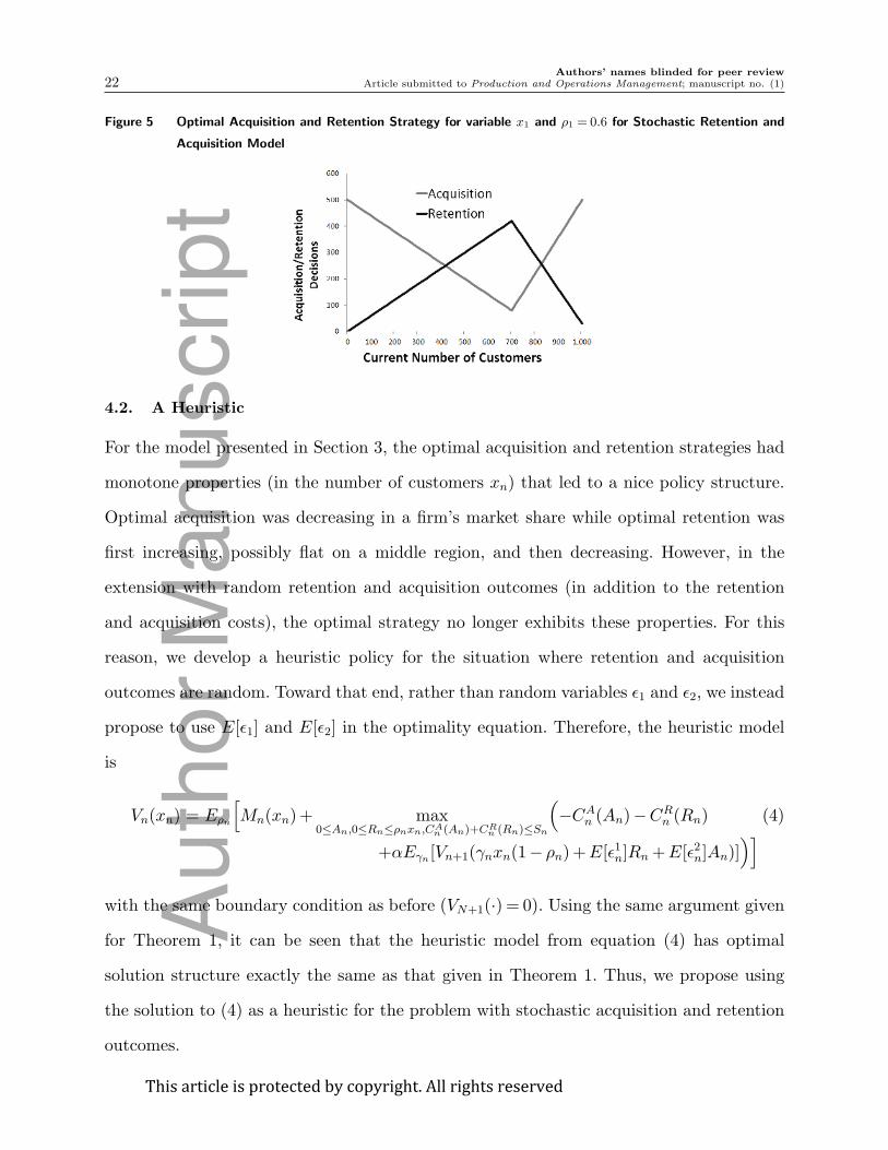
illustrates some of these phenomena; the optimal acquisition and retention strategies are
given in Figure 5, which is in contrast to the optimal policy structures from Theorem 1
displayed in Figure 1 and 2.
Example 2. This example is generated by modifying data from (Chen et al. 2012). Again
we consider a problem with two periods, N = 2, hence V2(·) =M2(·). The revenue function
is piece-wise linear and concave, where the firm makes 14 dollars for each customer up to
500, and half a dollar for customers thereafter, i.e.,
M2(x2) =
{
14x2, if x2 ≤ 500;
7000+0.5(x2 − 500), if x2 > 500,
and the acquisition and retention costs are linear:
C1(A1) = 2.5A1, D1(R1) = 3.6R1.
The three random variables are assumed to be discrete: γn = 0 and 1 with probabilities 1/2
and 1/2; ǫ1n = 0.5 and 1 with probabilities 1/2 and 1/2; and ǫ2n = 0.2 and 1 with probabilities
1/2 and 1/2. We fix parameter ρ1 = 0.6 and assume that S1 is sufficiently large such that
the cash constraint does not factor into the decision-making. We study how the strategy
varies in the initial number of customers at the beginning of period 1, x1.
The optimal strategies are presented in Figure 5. One can see that acquisition is no
longer decreasing in x1, which was our insight for the previous model. The intuition for
this phenomenon is the following. When x1 is small, the firm prefers the more certain
strategy of retention, and invests up to the upper bound of the constraint on retention.
The firm prefers the certain strategy because that increases the chances to get to x2 = 500,
which is where the marginal customer value changes. For high x1, the firm already has
good chance of getting up to x1 = 500, so it starts to prefer acquisition, which is more
uncertain, but slightly more cost effective. For this reason, we see that acquisition increases
while retention decreases. This lack of monotonicity is not surprising given the results in
the literature for inventory models with random yield and two suppliers (see Chen et al.
(2012)).
Thisarticleisprotectedbycopyright.Allrightsreserved
Auth
or
Manuscript
Authors’ names blinded for peer review
22 Article submitted to Production and Operations Management; manuscript no. (1)
Figure 5 Optimal Acquisition and Retention Strategy for variable x1 and ρ1 = 0.6 for Stochastic Retention and
Acquisition Model
4.2. A Heuristic
For the model presented in Section 3, the optimal acquisition and retention strategies had
monotone properties (in the number of customers xn) that led to a nice policy structure.
Optimal acquisition was decreasing in a firm’s market share while optimal retention was
first increasing, possibly flat on a middle region, and then decreasing. However, in the
extension with random retention and acquisition outcomes (in addition to the retention
and acquisition costs), the optimal strategy no longer exhibits these properties. For this
reason, we develop a heuristic policy for the situation where retention and acquisition
outcomes are random. Toward that end, rather than random variables ǫ1 and ǫ2, we instead
propose to use E[ǫ1] and E[ǫ2] in the optimality equation. Therefore, the heuristic model
is
Vn(xn) = Eρn
[
Mn(xn)+ max0≤An,0≤Rn≤ρnxn,CA
n (An)+CRn (Rn)≤Sn
(
−CAn (An)−CR
n (Rn) (4)
+αEγn [Vn+1(γnxn(1− ρn)+E[ǫ1n]Rn +E[ǫ2n]An)])]
with the same boundary condition as before (VN+1(·) = 0). Using the same argument given
for Theorem 1, it can be seen that the heuristic model from equation (4) has optimal
solution structure exactly the same as that given in Theorem 1. Thus, we propose using
the solution to (4) as a heuristic for the problem with stochastic acquisition and retention
outcomes.
Thisarticleisprotectedbycopyright.Allrightsreserved
Auth
or
Manuscript

Authors’ names blinded for peer review
Article submitted to Production and Operations Management; manuscript no. (1) 23
Table 1 Testing Scenario Overview (N = 5 and for all n, ρn = 0.1 and 0.2 with probabilities 0.5 and 0.5, CAn (An) =
An if An ≤ 100, and CAn (An) = 100 + 5(An − 100) if An > 100, and Sn sufficiently large. γn, ǫ
1n and ǫ2n
are distributed with equal probability across given values)
Parameter Option 1 Option 2 Option 3Revenue Function 6x0.65
n 6x0.8n -
Retention Cost 0.8Rn Rn 1.2Rn
γn Distribution (discrete uniform) {0.8,0.9} {0.8,0.9,1.0} {0.7,0.8,0.9,1.0}ǫ1n Distribution (discrete uniform) {0.6,0.9} {0.5,0.7,0.9} {0.6,0.7,0.8,0.9}ǫ2n Distribution (discrete uniform) {0.5,0.8} {0.4,0.6,0.8} {0.4,0.5,0.6,0.7}
To understand the performance of this heuristic approach, we conducted a numerical
study on a number of different scenarios, and computed the performance of the heuristic
as compared to an optimal strategy. The parameters that we used in our numerical study
are summarized in Table 1. For all scenarios, we consider a five-period problem (N = 5),
and assume, for all n, that ρn = 0.1 and 0.2 with probabilities 1/2 and 1/2, CAn (An) =An
if An ≤ 100, and CAn (An) = 100+5(An−100) if An > 100. We also assume that the random
variables γn, ǫ1n and ǫ2n are distributed with equal probability across a number of different
values (discrete uniform distribution). Finally, we assume that the expected cash constraint
is Sn = 400 in each period of the model.
By varying the different parameters, we tested 162 different scenarios. We summarize
the results of the numerical study in Table 2. For each scenario, we determined the average
error (across a number of different possible starting states), and the worst error.
Table 2 Testing Summary
Metric PerformanceAverage Average Error 0.04 %Average Worst Error 0.31 %Worst Average Error 0.09 %Worst Worst Error 0.61 %
In each of the scenarios we tested, the average error was well under one tenth of a percent
with a maximum error under one percent. This indicates that our heuristic performs very
well with reasonable functions for acquisition/retention costs and benefits.
Thisarticleisprotectedbycopyright.Allrightsreserved
Auth
or
Manuscript

Authors’ names blinded for peer review
24 Article submitted to Production and Operations Management; manuscript no. (1)
Although our numerical study indicates that the heuristic generally performs well, it
is possible to also find examples where it does not. Consider once again our numerical
example in Subsection 4.1. We compared the optimal strategy for this problem to the
heuristic across scenarios in which the number of starting customers x1 varied between
0 and 2000. In this case, the average error of the heuristic was 13.9 percent across all
scenarios with the worst error equal to 20.7 percent.
We note however that this is a highly contrived example where the firm’s revenue func-
tion has a severe discontinuity: the firm makes 14 dollars per customer up to 500 customers
but only 0.5 thereafter. Furthermore, while acquisition is less costly in expectation, reten-
tion outcomes are less random. Therefore when we replace the random outcomes by their
expectations, the heuristic only uses acquisition. This is to its detriment because the sharp
discontinuity in the revenue function rewards a strategy in which retention is used so
long as the number of customers is below 500. However, we were only able to generate
examples where the heuristic performed so poorly when our parameters had such dras-
tic changes and we believe that such situations are less likely in practice. In fact, with a
similar example and a more smooth revenue function, we see that the heuristic performs
well, a finding consistent with the results from our more comprehensive computational
testing. Suppose instead of making $14 up to 500 customers and then $0.50 thereafter, the
firm’s revenue function is piece-wise linear with decreasing marginal customer values of
14,12,11,10,9,8,7.5,7,6.5,6,5.5,5,4.5,4,3.5,3,2.5,2,1.5,1 (all in $) for the twenty 25-customer
increments from 0 to 500 (i.e. the firm makes $14 for each of the first 25 customers, then
$12 for each of the next 25, then $11 for the next 25, etc.). Above 500, we assume the
marginal customer value is $0.50 as before. In this case the heuristic performs well, with
the average profit across all cases equal to 0.75 percent and the worst error observed across
all cases equal to 3.42 percent. Again because firms’ revenue functions are likely smooth
in practice, we think this example is more realistic than the one where the firm’s marginal
revenue from customers went from $14 to $0.5 at a single sharp point. More generally, our
Thisarticleisprotectedbycopyright.Allrightsreserved
Auth
or
Manuscript
Authors’ names blinded for peer review
Article submitted to Production and Operations Management; manuscript no. (1) 25
numerical tests found that it is possible to find cases where the suggested heuristic does
not work well, but to generate these cases, one needed very sharp jumps in the revenue,
acquisition cost and retention cost functions. As seen in the above example, more gradual
jumps in these functions resulted in a pretty good performance for the heuristic.
5. Conclusion
Maintaining and growing a base of profitable customers is critical to the success of many
companies across different industries. To succeed, companies need to appropriately allocate
resources to the retention of existing customers and to acquisition of new ones. In this
paper we develop a model to analyze this problem which captures the practical interactive
dynamic decision-making process. Existing literature has focused on the acquisition and
retention trade-off using regression, empirical analysis, or static optimization. This work
is unique in that it provides a dynamic optimization perspective on the resource alloca-
tion trade-off between customers acquisition and retention. Because customer relationships
evolve over time, we believe the paper makes a meaningful contribution to the literature.
With some plausible assumptions on the costs of acquisition and retention and the
revenue generated from customers, we obtain some interesting structural properties for
the optimal strategy, which then provide important insights to the firm’s optimal solution.
For a small firm undergoing initial growth in its customer base, our results emphasize the
critical importance of customer retention; the firm should spend heavily on both channels,
while shifting resources from acquisition to retention during this initial growth. In practice,
we believe that many firms undervalue retention during initial growth of its customer base
and overemphasize acquisition. If this were to occur, acquisition can be undermined by the
loss of existing customers, stalling growth. When a firm gets larger, there may exist a region
in which the spending in acquisition and retention is flat because the firm is spending at
the maximal amount dictated by the cash constraint. Finally, when its customer base is
large enough the firm begins to invest less in both acquisition and retention. The reason
for this is that when retention efforts become prohibitively expensive, the firm accepts
Thisarticleisprotectedbycopyright.Allrightsreserved
Auth
or
Manuscript
Authors’ names blinded for peer review
26 Article submitted to Production and Operations Management; manuscript no. (1)
that it might lose some customers, rather than spending a lot of resource to try and
keep every customer. This important result is consistent with some observations in the
telecommunication industries. In practice, some customers may be so expensive to keep
satisfied that it no longer makes sense for the firm to continue retaining every one of them,
if the customer base is large enough. However, we also did find conditions that enable the
firm to continue growing: namely, if the firm can reduce acquisition and retention costs
over time, or if the firm can increase the value of its customers by convincing the customers
to buy more services, then it is optimal for the firm to continue growing its customer base
over time. We also discussed an extension to our model where acquisition and retention
outcomes (as well as their costs) are random. This case results in a much more complex
optimal policy structure and we developed an effective heuristic policy for that.
There is significant opportunity for additional research from the operations management
community on the topic of customer acquisition and retention management. For example,
it is often the case in practice that multiple firms target the same pool of prospective
customers, and one would need to apply game theory to study the dynamic decision making
and competition of the firms. There is also the possibility of incorporating other sales
management decisions into the framework of the acquisition and retention trade-off. For
example, one may consider joint decisions on acquisition, retention, and sales compensation
design, or joint decisions on acquisition, retention, and hiring or laying-off employees.
Such models would extend our work to consider other strategic aspects of the dynamic
acquisition and retention management problem.
Acknowledgment: The authors are grateful to the Senior Editor and two referees and their
constructive comments and suggestions, which have helped to significantly improve both
the content and exposition of this paper.
References
Ahn, H.S., T. Olsen. 2011. Inventory competition with subscriptions. Working Paper.
Thisarticleisprotectedbycopyright.Allrightsreserved
Auth
or
Manuscript

Authors’ names blinded for peer review
Article submitted to Production and Operations Management; manuscript no. (1) 27
Blattberg, R., J. Deighton. 1996. Manage marketing by the customer equity test. Harvard Business Review
74(4) 136–144.
Chen, F. 2005. Salesforce incentives, market information, and production/inventory planning. Management
Science 51(1) 60–75.
Chen, W., Q. Feng, S. Seshadri. 2012. Sourcing from suppliers with random yield for price dependent
demand. Annals of Operations Research to appear.
Dong, Y., Y. Yao, T. Cui. 2011. When acquisition spoils retention: Direct selling vs. delegation under crm.
Management Science 57(7) 1288–1299.
Fruchter, G. E., Z. J. Zhang. 2004. Dynamic targeted promotions. Journal of Service Research 7(1) 3–19.
Gonik, J. 1978. Tie saleman’s bonuses to forecasts. Harvard Business Review 56(1) 116–123.
Grossman, S.J., O.D. Hart. 1983. An analysis of the principal-agent problem. Econometrica 51(1) 7–45.
Gupta, A. K, K.G. Smith, C.E. Shalley. 2006. The interplay between exploration and exploitation. Academy
of Management Journal 49(4) 693–706.
Hall, J., E. Porteus. 2000. Customer service competition in capacitated systems. Manu. and Service Oper.
Management 2(2) 144–165.
Heyman, D., M. Sobel. 2004. Stochastic Models in Operations Research Vol II . Dover Publications.
Holmstrom, B. 1979. Moral hazard and observability. Bell Jounal of Economics 10(1) 74–91.
Homburg, C., V. Steiner, D. Totzek. 2009. Managing dynamics in a customer portfolio. Journal of Marketing
73(5) 70–89.
March, J.G. 1991. Exploration and exploitation in organizational learning. Organizational Science 2(1)
71–87.
Matos, C. A., J. L. Henrique, C. A. Rossi. 2007. Service recovery paradox: A meta-analysis. Journal of
Service Research 10(1) 60–77.
Olsen, T., R. Parker. 2008. Inventory management under market size dynamics. Management Sci. 54(1)
1805–1821.
Porteus, E., S. Whang. 1991. On manufacturing/marketing incentives. Management Science 37(9) 1166–
1181.
Raju, J., V. Srinivasan. 1996. Quota-based compensation plans for multiterritory heterogeneous salesforces.
Management Science 42(10) 1454–1462.
Reinartz, W., J. Thomas, V. Kumar. 2005. Balancing acquisition and retention resources to maximize
customer profitability. Journal of Marketing 69(1) 63–79.
Shavell, S. 1979. Moral hazard and observability. Quarterly Jounal of Economics 93(4) 541–562.
Spreng, R. A., G. D. Harrell, R. D. Mackoy. 1995. Service recovery: Impact on satisfaction and intentions.
Journal of Services Marketing 9(1) 15–23.
Thisarticleisprotectedbycopyright.Allrightsreserved
Auth
or
Manuscript

Authors’ names blinded for peer review
28 Article submitted to Production and Operations Management; manuscript no. (1)
Thomas, J. 2001. A methodology for linking customer acquisition to customer retention. Journal of Marketing
Research 38(2) 262–268.
Topkis, D. 1998. Supermodularity and Complementarity . Priceton University Press.
Appendix
In this appendix, we present all the technical proofs. Throughout the proofs we define R∗n(xn, ρn) and
A∗n(xn, ρn) to be the optimal solutions for the variables Rn and An, given that the number of customers at
the beginning of period n is xn and the observed fraction of unhappy customers is ρn.
Proof of Lemma 1. The problem we are studying is
maxx≥0,y≥0
f(x)+ g(y)+E[h(x+ y+ ǫK)], (5)
and we have continuity and strict concavity assumptions on the three functions and that both constant K
and random variable ǫ are non-negative.
Rewrite (5) as
maxz≥0
(
D(z)+E[h(z+ ǫK)])
(6)
with
D(z) = max0≤x≤z
(
f(x)+ g(z− y))
. (7)
The optimization problem in (6) is submodular in (z,K) because ǫ is non-negative, thus the optimal solution,
denoted by z∗(K), is decreasing in K. From the problem given in (7), the maximand is supermodular in
(x, z) and the constraint 0≤ x≤ z is a lattice, hence the optimal x∗ is increasing in z. Considered together,
this implies that a smaller value of K results in a larger value of z and a larger value of x. Therefore, x∗(K)
is decreasing in K. We rewrite (7) as
D(z) = max0≤y≤z
(
f(z− y)+ g(y))
. (8)
Using this equation (8) and the supermodularity in (z, y) we similarly obtain that the optimal y, denoted by
y∗(K), is decreasing in K.
To show that the slopes of the optimal x∗(K) and y∗(K) are between -1 and 0, we argue that the optimal
z∗(K) has slope between 0 and -1. This is sufficient to conclude the same about x∗(K) and y∗(K) because,
by the fact that each is decreasing in K, and x∗(K) + y∗(K) = z∗(K), it would be impossible for one of
x∗(K) and y∗(K) to decrease by more than that of z∗(K).
Suppose that K increases by c > 0, but z∗ decreases by d > c. This condition is formally written as
z∗(K + c) = z∗(K)− d < z∗(K)− c. We argue such a situation cannot occur because if true, we are able to
find a very small δ > 0, such that z∗(K + c) + δ is a strictly better solution than z∗(K + c). We argue this
Thisarticleisprotectedbycopyright.Allrightsreserved
Auth
or
Manuscript

Authors’ names blinded for peer review
Article submitted to Production and Operations Management; manuscript no. (1) 29
solution is better by the following inequalities. Note that it is easy to see from (7), that D(·) in equation (6)
is convex.
D(Z∗(k)− d+ δ)−D(Z∗(K)− d)
< D(z∗(K))−Dn(z∗(K)− δ)
≤ E[h(z∗(K)+ ǫK − δ)]−E[h(z∗(K)+ ǫK)]
≤ E[h(z∗(K)− d+ ǫ(K + c))]−E[h(z∗(K)− d+ δ+ ǫ(K + c))],
where the first inequality comes from the convexity of D(·), the second from the optimality of the solution
z∗(K), and the third from the convexity of h(·) along with the fact that we can pick δ small enough so that
cǫ− d+ δ≤ 0. Considering the first and last expressions, we see that
E[h(z∗(K)− d+ δ+ ǫ(K + c))] +D(Z∗(k)− d+ δ)>E[h(z∗(K)− d+ ǫ(K + c))] +D(Z∗(K)− d),
contradicting the optimality of the original solution.
Thus, the analysis above shows that the optimal x∗(K) and y∗(K) are decreasing in K, but with slopes
between -1 and 0.
Proof of Theorem 1. The optimality equation is
Vn(xn) =Eρn
[
Mn(xn) (9)
+ max0≤Rn≤xnρn,0≤An,CA
n(An)+CR
n(Rn)≤Sn
(
−CAn (An)−CR
n (Rn)+E[αVn+1(γnxn(1− ρn)+Rn +An)])]
.
First note that, for any given selections of An, Rn, and an outcome ρn, the objective function of the
maximization problem on the right hand side of (10) is increasing in xn, and the feasible region is strictly
larger for larger xn, thus after maximization it is also increasing in xn. Then, by the assumption that Mn(xn)
is increasing, we conclude that Vn(xn) is increasing in xn.
The concavity of Vn(xn) follows by concavity preservation. By Assumptions 1 and 2, on CAn (·) and CR
n (·),
and the induction hypothesis on Vn+1(.), the objective function of the maximization problem on the right
hand side of (10) is jointly concave in (An,Rn, xn). Because the feasible region constitutes a convex set, it
follows from Heyman and Sobel (2004) that Vn(xn) is a concave function.
To characterize the optimal policy, we consider the unconstrained optimization problem by relaxing the
constraint in (10) as follows:
Un(xn, ρn) =Mn(xn)+ max0≤An,0≤Rn
(
−CAn (An)−CR
n (Rn)+αVn+1(γnxn(1− ρn)+Rn +An))
. (10)
We will call this the relaxed problem, and use it for subsequent analysis. Note the difference between this
problem and the original problem: problem (10) does not have either constraint Rn ≤ xnρn or CAn (An) +
CRn (Rn)≤ Tn, and it assumes the fraction of unhappy customer ρn is known.
Thisarticleisprotectedbycopyright.Allrightsreserved
Auth
or
Manuscript

Authors’ names blinded for peer review
30 Article submitted to Production and Operations Management; manuscript no. (1)
Now we can use Lemma 1 to argue the following property on the relaxed problem: The optimal solution to
the problem Un(xn, ρn), which we denote by (AU∗n (xn(1−ρn)),R
U∗n (xn(1−ρn)), is decreasing in the expression
xn(1− ρn), with slope between 0 and -1. This is an immediate application of Lemma 1, simply by switching
from maximization to minimization and corresponding An and Rn to x and y and the functions CAn (·), C
Rn (·),
and −Vn(·) to f(·), g(·) and h(·). The expression xn(1− ρn) plays the role of the constant K.
Based on the problem given in (10) with decreasing solution vector (AU∗n (xn(1−ρn)),R
U∗n (xn(1−ρn)), we
define the following value,
Kn = {w :CAn (A
U∗n (w))+CR
n (RU∗n (w)) = Sn}, (11)
which will be useful in establishing the main result. If such a value Kn does not exist, we we set Kn = 0.
Next we consider a second intermediary problem in which we consider only the cash constraint, but not
the upper bound on retention. This problem is
Yn(xn(1− ρn)) (12)
= Mn(xn)+ max0≤An,0≤Rn,CA
n(An)+CR
n(Rn)≤Sn
(
−CAn (An)−CR
n (Rn)+αVn+1(γnxn(1− ρn)+Rn +An))
.
In what follows we show that the solution to (12) is
(AY ∗n (xn(1− ρn)),R
Y ∗n (xn(1− ρn))) = (AU∗
n (xn(1− ρn)),RU∗n (xn(1− ρn))
if xn(1− ρn)≥Kn and otherwise, it is
(AY ∗n (xn(1− ρn)),R
Y ∗n (xn(1− ρn))) = (AU∗
n (Kn),RU∗n (Kn)).
First consider the case when xn(1−ρn)≥Kn. In this situation, because AU∗n (·) and RU∗
n (·) are decreasing,
we are able to show the following:
CAn (A
U∗n (xn(1− ρn)))+CR
n (RU∗n (xn(1− ρn))≤CA
n (AU∗n (Kn))+CR
n (RU∗n (Kn)) = Tn.
Therefore in this case the solution from (10) is feasible for (12), so it is also optimal for (12).
Now suppose instead that xn(1− ρn)<Kn, we want to show, by contradiction, that the optimal solution
pair is (AU∗n (Kn),R
U∗n (Kn)). Suppose for some xn(1− ρn)<Kn, we have an optimal strategy of AY ∗
n (xn(1−
ρn)) and RY ∗n (xn(1− ρn)) which are not equal to AU∗
n (Kn) and RU∗n (Kn) respectively. In the following we
show that this would lead to contradiction.
Consider several cases. First, suppose
AY ∗n (xn(1− ρn))+RY ∗
n (xn(1− ρn))>AU∗n (Kn)+RU∗
n (Kn). (13)
This would contradict the optimality of the solution pair AU∗n (Kn) and RU∗
n (Kn), by the following arguments:
−CAn (A
U∗n (Kn))−CR
n (RU∗n (Kn))+E[Vn+1(γnKn +AU∗
n (Kn)+RU∗n (Kn))]
=−Sn +E[Vn+1(γnKn +AU∗n (Kn)+RU∗
n (Kn))]
<−Sn +E[Vn+1(γnKn +AY ∗n (xn(1− ρn))+RY ∗
n (xn(1− ρn)))]
Thisarticleisprotectedbycopyright.Allrightsreserved
Auth
or
Manuscript
Authors’ names blinded for peer review
Article submitted to Production and Operations Management; manuscript no. (1) 31
≤−CAn (A
Y ∗n (xn(1− ρn)))−CR
n (RY ∗n (xn(1− ρn)))
+E[Vn+1(γnKn +AY ∗n (xn(1− ρn))+RY ∗
n (xn(1− ρn)))],
where the equality follows form the definition of Kn, the first inequality follows from the strict monotonicity
of the value function Vn+1(·), and the second follows from the fact that the cash constraint must be satisfied
by AY ∗n (xn(1−ρn)) and RY ∗
n (xn(1−ρn)). Looking at the first and last expressions, the firm is strictly better
off switching strategies from the pair AU∗n (Kn) and RU∗
n (Kn) to the pair AY ∗n (xn(1−ρn)) and RY ∗
n (xn(1−ρn)),
which contradictions the optimality of the first solution pair.
Next, suppose that AY ∗n (xn(1− ρn)) +RY ∗
n (xn(1− ρn)) < AU∗n (Kn) +RU∗
n (Kn). We will prove that this
contradicts the optimality of the solution pair AY ∗n (xn(1− ρn)) and RY ∗
n (xn(1− ρn)). Note that
CAn (A
U∗n (Kn))+CR
n (RU∗n (Kn))−CA
n (AY ∗n (xn(1− ρn)))−CR
n (RY ∗n (xn(1− ρn)))
≤ E[Vn+1(γnKn +AU∗n (Kn)+RU∗
n (Kn))]−E[Vn+1(γnKn +AY ∗n (xn(1− ρn))+RY ∗
n (xn(1− ρn)))]
< E[Vn+1(γnxn(1− ρn)+AU∗n (Kn)+RU∗
n (Kn))]
−E[Vn+1(γnxn(1− ρn)+AY ∗n (xn(1− ρn))+RY ∗
n (xn(1− ρn)))],
where the first inequality comes from the optimality of the solution with Kn, and the second inequality
follows from the concavity of the value function because xn(1− ρn) < Kn. Considering the first and last
expressions together, we conclude that AU∗n (Kn) and RU∗
n (Kn) is a strictly better solution, contradicting the
optimality of the solution pair of AY ∗n (xn(1− ρn)) and RY ∗
n (xn(1− ρn)).
The final case is
AY ∗n (xn(1− ρn))+RY ∗
n (xn(1− ρn)) =AU∗n (Kn)+RU∗
n (Kn), (14)
but AY ∗n (xn(1− ρn)) 6= AU∗
n (Kn) and RY ∗n (xn(1− ρn)) 6= RU∗
n (Kn). Let AY ∗n (xn(1− ρn))−AU∗
n (Kn) = δ, so
that it is also true that RY ∗n (xn(1− ρn))−RU∗
n (Kn) =−δ. We first prove that
−CAn (A
U∗n (Kn)+ δ)−CR
n (RU∗n (Kn)− δ))<−CA
n (AU∗n (Kn))−CR
n (RU∗n (Kn)))]. (15)
Suppose instead that
−CAn (A
U∗n (Kn)+ δ)−CR
n (RU∗n (Kn)− δ))>−CA
n (AU∗n (Kn))−CR
n (RU∗n (Kn)).
Then this would contradict the optimality of the solution pair AU∗n (Kn) and RU∗
n (Kn), because the alternative
solution of AU∗n (Kn) + δ and RU∗
n (Kn) − δ would have strictly lower cost with identical impact on the
expression inside of Vn+1(·), due to the given condition that AY ∗n (xn(1−ρn))+RY ∗
n (xn(1−ρn)) =AU∗n (Kn)+
RU∗n (Kn). Hence, let us next suppose
−CAn (A
U∗n (Kn)+ δ)−CR
n (RU∗n (Kn)− δ)) =−CA
n (AU∗n (Kn))−CR
n (RU∗n (Kn)). (16)
We propose an alternative solution, with strictly lower cost, again with identical impact on the expression
inside of Vn+1(·) (thus, again contradicting the optimality of the given solutions). This solution isAU∗n (Kn)+
δ
2
and RU∗n (Kn)−
δ
2. Then,
−CAn
(
AU∗n (Kn)+
δ
2
)
−CRn
(
RU∗n (Kn)−
δ
2
)
Thisarticleisprotectedbycopyright.Allrightsreserved
Auth
or
Manuscript

Authors’ names blinded for peer review
32 Article submitted to Production and Operations Management; manuscript no. (1)
>−1
2CA
n (AU∗n (Kn))−
1
2CR
n (RU∗n (Kn))−
1
2CA
n (AU∗n (Kn)+ δ)−
1
2CR
n (RU∗n (Kn)− δ))
=CAn (A
U∗n (Kn))−CR
n (RU∗n (Kn)),
where the inequality follows from the strictly convexity of the cost functions in Assumption 1, and the
equality follows from (16). So in this case we again contradict the optimality of AU∗n (Kn) and RU∗
n (Kn),
because the proposed solution of AU∗n (Kn) +
δ
2and RU∗
n (Kn)−δ
2has strictly lower cost and with identical
impact on the expression inside of Vn+1(·).
Consequently, we have
−CAn (A
Y ∗n (xn(1− ρn)))−CR
n (RY ∗n (xn(1− ρn)))
+E[Vn+1(xn(1− ρn)+AY ∗n (xn(1− ρn))+RY ∗
n (xn(1− ρn)))]
=−CAn (A
U∗n (Kn)+ δ)−CR
n (RU∗n (Kn)− δ))+E[Vn+1(xn(1− ρn)+AY ∗
n (Kn)+RU∗n (Kn))]
<−CAn (A
U∗n (Kn))−CR
n (RU∗n (Kn)))+E[Vn+1(xn(1− ρn)+AY ∗
n (Kn)+RU∗n (Kn))]
=−CAn (A
U∗n (Kn))−CR
n (RU∗n (Kn)))+E[Vn+1(xn(1− ρn)+AY ∗
n (xn(1− ρn))+RY ∗n (xn(1− ρn))],
where the inequality follows from (15), and the second equality follows from condition (14). This contradicts
the optimality of the solution pair AY ∗n (xn(1− ρn)) and RY ∗
n (xn(1− ρn)).
Summarizing the analysis above, we have shown that the solution to (12) is given by (AY ∗n (xn(1 −
ρn)),RY ∗n (xn(1 − ρn)) = (AU∗
n (xn(1 − ρn)),RU∗n (xn(1 − ρn)) if xn(1 − ρn) ≥ Kn, and it is (AY ∗
n (xn(1 −
ρn)),RY ∗n (xn(1− ρn))) = (AU∗
n (Kn),RU∗n (Kn)) otherwise.
We are now ready to prove Theorem 1. We first prove (i). Note that the relaxed problem (12) repre-
sents the optimization in problem (10) without constraint Rn ≤ ρnxn. Writing the optimization problem as
sequential optimization of An and Rn respectively, it follows from the joint concavity in (An,Rn) that the
objective function after optimizing An is a concave function of Rn. Since the resulting objective function
after optimizing An in (12) is concave in Rn with maximizer RY ∗n (xn(1− ρn)), it is clear that the optimal
solution of the original value function in (2) is RY ∗n (xn(1− ρn)) when RY ∗
n (xn(1− ρn)) ≤ ρnxn and , and
otherwise it is ρnxn.
Because RY ∗n (xn(1− ρn))≥ 0 is decreasing in xn, as xn increases, there must exist a unique point where
RY ∗n (xn(1− ρn)) = xnρn, which establishes the existence of Qn(ρn) from the theorem, defined by
Qn(ρn) = sup{
xn ≥ 0; ρnxn ≤RY ∗n (xn(1− ρn))
}
, (17)
such that as xn ≤Qn(ρn) it holds that RY ∗n (xn(1−ρn))> ρnxn; while if xn >Qn(ρn) then RY ∗
n (xn(1−ρn))≤
ρnxn.
Combining this insight with the characterization of the optimal policy RY ∗n (xn(1−ρn)) given above yields
the optimal retention policy as stated in the theorem, which is to set Rn to ρnxn if xn ≤Qn(ρn), set Rn to
RU∗n (Kn) if xn ∈ (Qn(ρn),
Kn
ρn) and set Rn to RU∗
n (xn(1− ρn)) otherwise. Note that the second region might
be empty.
Thisarticleisprotectedbycopyright.Allrightsreserved
Auth
or
Manuscript
Authors’ names blinded for peer review
Article submitted to Production and Operations Management; manuscript no. (1) 33
To find the optimal acquisition strategy, we let AW∗
n (.) be defined as the maximizer of
Wn(xn, ρn) = max0≤An
(
−CAn (An)+E[Vn+1(γnxn(1− ρn)+ ρnxn +An)])
)
. (18)
By the same analysis as above, it can be seen that AW∗n (xn, ρn) is also decreasing in xn but with slope no
less than -1. Note that on the range xn ≤Qn(ρn), the optimization problem for An in (2) can be written as
max0≤An
(
−CAn (An)−CR
n (ρnxn)+αVn+1(γnxn(1− ρn)+ ρnxn +An))
,
and its optimal solution is AW∗n (xn, ρn) just defined in (18).
With these quantities defined, we can discuss the optimal acquisition strategy on the regions discussed
above. When xn ≤ Qn(ρn) and Rn = ρnxn, then the optimal An is AW∗n (xn, ρn), conditional on that it is
within cash constraint. If not, by the convexity of the problem given in (18), the best solution is at the
truncated solution. Thus, the optimal An on this region is min{AW∗n (xn, ρn), Tn −CR
n (ρnxn)}. When xn ∈
(Qn(ρn),Kn/ρn), the optimal solution is the one discussed in problem (12), which is AU∗n (Kn). In all other
cases, the optimal solution is given by AU∗n ((1− ρn)xn).
The argument that Qn(ρn) is decreasing follows from the fact that RY ∗n (xn(1 − ρn)) is decreasing in
xn(1−ρn) with slope between -1 and 0, and the definition of Qn(ρn) in (17). To see that, suppose ρn were to
increase by a positive number s > 0, then ρnxn would increase by sxn, while RY ∗n (xn(1−ρn)) would increase
by a value between 0 and sxn. Therefore to reach equality once again, one would need to decrease xn. This
establishes that Qn(ρn) is decreasing in ρn.
We next prove (ii). From part (i), we know that the optimal decision in acquisition is decreasing in xn.
Therefore, either eventually A∗n(xn, ρn) = 0, or this value is infinite, establishing the existence of QA
n (ρn) (pos-
sibly infinity). Likewise, retention spending is first increasing, and then decreasing, so eventually R∗n(xn, ρn)
may reach 0, showing that QRn (ρn) exists (also possibly infinity). Both are increasing in ρn, because the
curves RU∗n (xn(1− ρn)) and AU∗
n (xn(1− ρn)) are increasing in ρn.
To establish part (iii), we need to argue that the following expression
xn+1 −xn = xn(1− ρn)γn +R∗n(xn, ρn)+A∗
n(xn, ρn)−xn (19)
is decreasing in xn for any given ρn and γn, where R∗n(xn, ρn) and A∗
n(xn, ρn) are the optimal retention
and optimal acquisition decision of the original problem, which are given according to cases above. Since
A∗n(xn, ρn) is decreasing while R∗
n(xn, ρn) first increases with slope ρn and then decreases, we conclude that
the terms combined must be decreasing in xn.
When xn = 0, the firm can only gain customers, and then the change in number of customers is decreasing
for xn > 0. Therefore there must exist a non-zero point x∗n(ρn) such that
E[xn+1]−xn =
{
≤ 0 if xn ≥ x∗n(ρn);
≥ 0 if xn ≤ x∗n(ρn).
This completes the proof of the optimal strategy. Note that it is possible that x∗n(ρn) =∞.
Thisarticleisprotectedbycopyright.Allrightsreserved
Auth
or
Manuscript

Authors’ names blinded for peer review
34 Article submitted to Production and Operations Management; manuscript no. (1)
Proof of Lemma 2.
We prove by contradiction. Suppose that (CAn )
′(0) < (CRn )
′(0), but QAn (ρn) < QR
n (ρn) for some ρn. This
implies that for such a ρn, and values of xn ∈ (QAn ,Q
Rn ), the firm has a strategy where A∗
n = 0 with R∗n > 0.
In this case, we show that there exists a small value δ > 0, such that a better solution is An = δ, with
Rn = R∗n − δ. Because this strategy has the same impact in Vn+1(·), we need only argue that it has lower
cost. The new solution would surely satisfy the cash constraint if it is indeed lower cost.
First we observe that because CRn (·) is strictly convex, and (CA
n )′(0)< (CR
n )′(0), it holds that as δ > 0 is
small enough we have
CRn (R
∗n)−CR
n (R∗n − δ)>CR
n (δ)−CRn (0)>CA
n (δ)−CAn (0). (20)
These inequalities show the existence of solution An = δ and Rn = R∗n − δ, which as strictly lower cost,
and same impact on future periods. This contradicts the original optimality of our solution. A symmetric
argument establishes that (CAn )
′(0)> (CRn )
′(0) implies that QAn (ρn)≤QR
n (ρn).
We finally consider the case (CAn )
′(0) = (CRn )
′(0), and prove that in this case it must hold that QAn (ρn) =
QRn (ρn) for all ρn > 0. Suppose QA
n (ρn) 6= QRn (ρn) for some ρn. Without loss of generality, suppose 0 ≤
QAn (ρn) < QR
n (ρn). This implies that there exists an xn ∈ (QAn (ρn),Q
Rn (ρn)), such that R∗
n(xn, ρn) > 0 and
A∗n(xn, ρn) = 0. We claim that there exists a small number δ > 0, such that a solution withRn =R∗
n(xn, ρn)−δ,
and An = δ is strictly superior. This would contradict the optimality of the original solution.
Observe that by the strict convexity of CRn (·), we have that:
(CRn )
′(R∗n(xn, ρn))> (CR
n )′(0) = (CA
n )′(0).
Therefore, by continuity we can find a small δ > 0 such that
(CRn )
′(R∗n(xn, ρn)− δ)> (CA
n )′(δ).
This implies, by convexity of CRn (·) and CA
n (·), that
CRn (R
∗n(xn, ρn))−CR
n (R∗n(xn, ρn)− δ)>CA
n (δ)−CAn (0).
Since solutions Rn =R∗n(xn, ρn)− δ and An = δ have the same impact to future periods, this proves that the
proposed solution has strictly lower cost, contradicting the optimality of the original solution. A symmetric
argument holds to contradiction if it were true that 0≤QRn (ρn)<QA
n (ρn).
Proof of Corollary 1.
The fact that limxn+1→∞M ′n+1(xn+1)≥ κ> 0, allows us to prove that the value function is κ increasing in
period n+1, meaning that Vn+1(xn+1 + s)−Vn+1(xn+1)≥ sκ for any s > 0. We can see this from the value
function as follows.
E[Vn+1(xn+1 + s)]−E[Vn+1(xn+1)] =E[Mn+1(xn+1 + s)]−E[Mn+1(xn+1)]
Thisarticleisprotectedbycopyright.Allrightsreserved
Auth
or
Manuscript

Authors’ names blinded for peer review
Article submitted to Production and Operations Management; manuscript no. (1) 35
+E[
max0≤Rn+1≤(xn+1+s)ρn+1,0≤An+1
(−CAn+1(An+1)−CR
n+1(Rn+1)
+αE[Vn+2((xn+1 + s)(1− ρn+1)γn+1 +Rn+1 +An+1)])]
−E[
max0≤Rn+1≤xn+1ρn+1,0≤An+1
(−CAn+1(An+1)−CR
n+1(Rn+1)
+αE[Vn+2(xn+1(1− ρn+1)γn+1 +Rn+1 +An+1)])]
≥ sκ,
where the last inequality comes from the fact that Mn+1(xn+1+s)−Mn+1(xn+1)≥ sκ, while the other terms
are non-negative, because Vn+2(·) is increasing, and the case with s+xn+1 has a larger feasible region.
By contradiction we now show that a point at which R∗n(xn, ρn) = 0 can never exist unless ρnxn = 0
or (CRn )
′(0) ≥ (CAn )
′((CAn )
−1(Sn)), because the firm is better off by spending a small incremental amount
more in retention. Suppose, on the contrary, it holds that the optimal strategies (R∗n(xn, ρn),A
∗n(xn, ρn)) has
R∗n(xn, ρn) = 0. We will show that in this case there exists a small δ > 0 such that the solution would be
improved ifR∗n(xn, ρn) = δ, contradicting the optimality of the original solution. This additional small increase
is feasible because of our two conditions, which say that the retention constraint is not tight with given
decision (because ρnxn > 0, and neither is the cash constraint (because if (CRn )
′(0)< (CAn )
′((CAn )
−1(Sn)) with
total acquisition and retention spending at Sn, the firm could save by shifting some money from acquisition
to retention). Using the fact that Vn+1(·) is κ increasing, we have
CRn (δ)−CR
n (0) < δακ (21)
≤ αE[Vn+1(xn(1− ρn)γn + δ+A∗n(xn, ρn))]−αE[Vn+1(xn(1− ρn)γn +A∗
n(xn, ρn))]. (22)
These inequalities follow from the fact that CRn (·) is strictly convex, (CR
n )′(0)≤ ακ, and Vn+1(·) is κ increasing,
as we have discussed.
The inequalities (21) implies that a strategy of no retention and A∗n(xn, ρn)) is acquisition is strictly
dominated by one with the same acquisition and a small amount δ > 0 in retention, contradicting the
optimality of former solution. This implies QRn (ρn) =∞.
Proof of Corollary 2.
Due the symmetric relationship between An and Rn, similar argument as those of Corollary 1 can be used
to prove this result. We omit the details.
Proof of Theorem 2.
The optimality equation for this more general case is
Vn(xn)
= Eρn
[
Mn(xn)
+ max0≤An,0≤Rn≤ρnxn,CA
n(An)+CR
n(Rn)≤Sn
(
−CAn (An)−CR
n (Rn)+αE[
Vn+1(γnxn(1− ρn)+ ǫ1nRn + ǫ2nAn)]
)]
.
The objective function of the maximization problem above is easily seen to be jointly concave in (An,Rn, xn),
and the constraint is a convex set of (An,Rn, xn), hence it follows from the preservation property that Vn(xn)
Thisarticleisprotectedbycopyright.Allrightsreserved
Auth
or
Manuscript

Authors’ names blinded for peer review
36 Article submitted to Production and Operations Management; manuscript no. (1)
is concave in xn. By induction, it is also easy to show that Vn(xn) is increasing in xn, since both the objective
function and the feasible region in the optimization are increasing in xn. Consider the relaxed problem that,
for any realization of ρn,
Yn(xn, ρn)
= Mn(xn)+ max0≤An,0≤Rn,CA
n(An)+CR
n(Rn)≤Sn
(
−CAn (An)−CR
n (Rn)+αE[
Vn+1(γnxn(1− ρn)+ ǫ1nRn + ǫ2nAn)]
)
= Mn(xn)+ max0≤Rn,CR
n(Rn)≤Sn
{
−CRn (Rn)+ g
(
(1− ρn)xn,Rn
)
}
,
where
g((1− ρn)xn,Rn) = max0≤An,CA
n(An)+CR
n(Rn)≤Sn
(
−CAn (An)+αE
[
Vn+1(γnxn(1− ρn)+ ǫ1nRn + ǫ2nAn)]
)
is jointly concave in ((1−ρn)xn,Rn). Therefore, if the optimal RY ∗n (xn, ρn)< ρnxn, then the solution the the
relaxed problem is feasible, thus it optimal. Otherwise by joint concavity, the optimal solution is (An,Rn) =
(AW∗n (xn, ρn), ρnxn), where AW∗
n is the optimal solution of
Wn(xn, ρn) = max0≤An,CA
n(An)≤Sn−CR
n(ρnxn)
(
−CAn (An)+αE
[
Vn+1(γnxn(1− ρn)+ ǫ1nρnxn + ǫ2nAn)]
)
. (23)
This finishes the proof for Theorem 2.
Thisarticleisprotectedbycopyright.Allrightsreserved
Auth
or
Manuscript