Dynamic Dependence in Corporate Credit∗

Peter Christoffersen Kris Jacobs

The Rotman School, University of Houston

CBS and CREATES and Tilburg University

Xisong Jin Hugues Langlois

University of Luxembourg McGill University

April 15, 2013

Abstract

Characterizing the dependence in credit spreads and default intensities across companiesis a central problem in credit risk. Existing practice typically relies on factor modelsor simple static Gaussian copula models. We instead use genuinely dynamic copulamodels which can capture univariate and multivariate non-normalities and asymmetriesfor large cross-sections of firms. Using weekly data for over nine years on 223 firms, wefind that the dependence in default intensities and CDS spreads is highly time-varyingand persistent, and it increases significantly in the financial crisis. The dependencebetween equity returns also increases in the financial crisis, but this increase is much lesspersistent. We document substantial multivariate non-normalities for CDS spreads anddefault intensities, but multivariate asymmetries are less important for credit than theyare for equities. The increase in cross-sectional dependence during the financial crisishas substantially reduced diversification benefits from selling credit protection, and itis critical to take non-normality into account when computing these benefits. Thesefindings have important implications for the management of portfolio credit risk, thepricing of structured credit products, and the role of credit-risky securities in diversifiedportfolios.

JEL Classification: G12

Keywords: credit risk; default risk; CDS; dynamic dependence; copula.

∗Correspondence to: Kris Jacobs, C.T Bauer College of Business, University of Houston, 334 Melcher Hall,Tel: (713) 743-2826; Fax: (713) 743-4622; E-mail: kjacobs@bauer.uh.edu.

1

1 Introduction

Characterizing the dependence between credit-risky securities is of great interest for portfolio

management and risk management, but not necessarily straightforward because multivariate

modeling is notoriously diffi cult for large cross-sections of securities. In existing work, com-

putationally straightforward techniques such as factor models are often used to model corre-

lations for large portfolios; alternatively, simple rolling correlations or exponential smoothers

are used.

We use explicitly multivariate econometric models for the purpose of modeling credit

correlation and dependence. We use genuinely dynamic copula techniques that can capture

univariate and multivariate deviations from normality, as well as multivariate asymmetries.

We are able to apply these techniques to large cross-sections of firms by using recently proposed

econometric innovations. We perform our empirical analysis using weekly data on 5-year

Credit Default Swap (CDS) contracts for 223 constituents of the first 18 series of the CDX

North American investment grade index, which cover the period from March 20th, 2003 to

September 20th, 2012. Our 223 firms enter and leave the sample at different times, but

this can easily be accommodated by the estimation methodology we employ. We investigate

the dependence between CDS spreads as well as default intensities. We also analyze the

dependence in equity prices for comparison.

We proceed in three steps. The two first steps are univariate. In the first, we remove the

short-run dynamics from the raw data by estimating firm-by-firm ARMA models on weekly

log differences. In a second step, we estimate firm-by-firm variance dynamics on the residuals

from the first step. We use an asymmetric NGARCH model with an asymmetric standardized

t-distribution following Hansen (1994).1 Finally, in a third step we provide a multivariate

analysis using the copula implied by the skewed t-distribution in DeMarta and McNeil (2004).

Dynamic copula correlations are modeled based on the linear correlation techniques developed

by Engle (2002) and Tse and Tsui (2002).2 To alleviate the computational burden, we rely on

the composite likelihood technique of Engle, Shephard, and Sheppard (2008) and the moment

matching from Engle and Mezrich (1996). See Patton (2012) for a recent survey of copula

models.

We find that copula correlations in CDS spreads and default intensities vary substantially

over our sample, with a significant increase following the financial crisis in 2007. Equity corre-

lations also increase after 2007, but less significantly so, and the increase is not as persistent.

The increase in cross-sectional dependence is clearly important for the management of port-

1Engle (1982) and Bollerslev (1986) developed the first ARCH and GARCH models. Bollerslev (1990) firstcombined the GARCH model with a t-distribution.

2See Engle and Kroner (1995) for an early multivariate GARCH model and Engle and Kelly (2012) for asimplified dynamic correlation model.

2

folio credit risk and the relative pricing of CDO tranches with different seniority levels. Our

estimates indicate fat tails in the univariate credit distributions, but also multivariate non-

normalities for CDS spreads and default intensities. Multivariate asymmetries seem to be less

important for credit than for equities, confirming the results from threshold correlations.

We use our estimates to compute time-varying diversification benefits from selling credit

protection. We find that the increase in cross-sectional dependence following the financial

crisis has substantially reduced diversification benefits, similar to what happened in equity

markets. When computing diversification benefits, taking non-normality into account is more

important for credit than for equity.

The paper proceeds as follows. In Section 2 we briefly discuss CDS markets. We dis-

cuss how to extract default intensities from CDS spreads, ass well as existing techniques

for modeling credit dependence. Section 3 summarizes stylized facts in the CDS and equity

data. Section 4 presents the models and Section 5 discusses the empirical results. Section 6

concludes.

2 CDS Markets, Default Intensity and Dependence

In this section, we first briefly discuss CDS markets. We then explain how to extract de-

fault intensities from CDS spreads, and we discuss existing techniques for modeling default

dependence.

2.1 CDS Markets

A CDS is essentially an insurance contract, where the insurance event is defined as default by

an underlying entity such as a corporation or a sovereign country. Which events constitute

default is a matter of some debate, but for the purpose of this paper it is not of great impor-

tance. The insurance buyer pays the insurance provider a fixed periodical amount, expressed

as a “spread”which is converted into dollar payments using the notional principal—the size of

the contract. In case of default, the insurance provider compensates the insurance buyer for

his loss.

The CDS market exploded in size between 2000 and 2007, standing at over 55 Trillion $US

in notional principal in late 2007, according to the Bank for International Settlements. While

the CDS market has subsequently been reduced to approximately 27 Trillion $US in notional

principal as of June 2012, market size seems to have stabilized over the last two years after

a sharp drop during the financial crisis. Also, the decline in CDS market size is much less

significant than the decline for more complex credit derivatives, in particular structured credit

products. This suggests that CDS markets have survived the financial crisis, highlighting the

3

importance of a market for single-name default insurance.

One element of the success and resilience of CDS markets has been the creation of market

indexes consisting of CDSs, the CDX index in North America and the iTraxx index in Europe.

In our empirical work, we use all 226 constituents of the first 18 series of the CDX North

American investment grade index. The list of firms we use in our empirical analysis is provided

in Table 1 and we discuss the data in more detail in Section 3.

2.2 Extracting Default Intensities from CDS Premia

When studying dependence in the CDS market, the question arises what the dependence

analysis should focus on. The most obvious object of interest are the CDS spreads themselves.

However, the purpose of our paper is to better understand correlation between credit names,

as part of any portfolio consisting of CDS or other credit-risky securities, or underlying a

structured product such as a collateralized debt obligation (CDO). From this perspective, the

analysis of default intensities is of equal or greater importance than the analysis of spreads

themselves. For example, the standard valuation tool for CDOs is a Gaussian copula, and

the most important input into this analysis is the correlation between the default intensities

of the CDO constituents. We therefore analyze the dependence between intensities as well as

spreads. To better motivate the analysis of default intensities, it is necessary to understand

how they can be extracted from the CDS contracts based on the valuation formulas.

The valuation of CDS contracts, and the estimation of default intensities that relies on

this valuation, has been studied in several papers.3 Consider a given risk-neutral survival

probability q(t, T ). The premium on a CDS is the spread paid by the protection buyer

that equates the expected present value of default costs to be borne by the protection seller

(“floating leg”) to the expected present value of investing in the CDS (“fixed leg”). The value

of the fixed leg is the present value of the spread payments the protection seller receives from

the protection buyer, while the unknown floating leg comprises the potential payment by the

protection seller to the buyer.

Consider now a CDS contract with payment dates T = (T1, ..., TN), maturity TN , premium

P and notional 1. Denote the value of the fixed leg by VFixed(t, T, P ), the value of the floating

leg by VFloating(t), and the discount factors by D(t, Ti). At each payment date Ti, the buyer

has to pay τ(Ti−1, Ti)P to the seller, where τ(Ti−1, Ti) represents the time period between Ti−1

and Ti (T0 is equal to t). If the reference entity does not default during the life of the contract,

the buyer makes all payments. However, if default occurs at time s ≤ TN , the buyer has made

3The literature on CDS contracts has expanded rapidly. For theoretical work, see Das and Sundaram (2000)and Hull and White (2000). For empirical studies, see Berndt, Douglas, Duffi e, Ferguson, and Schranz (2004),Blanco, Brennan, and Marsh (2005), Ericsson, Jacobs and Oviedo (2009), Houweling and Vorst (2005), Hull,Predescu and White (2006), Longstaff, Mithal and Neiss (2004), and Zhang, Zhou and Zhu (2009).

4

I(s) payments, where I(s) = max(i = 0, ..., N : Ti < s) , and has to pay an accrual payment

of τ(TI(s), s)P at time s. Denote the probability density function associated with the default

intensity process ψt by fψ(t), and let the recovery rate be δ, then

VFixed(t, T, P ) = Pt

N∑i=1

D(t, Ti)τ(Ti−1, Ti)q(t, Ti) +

TN∫t

D(t, s)τ(TI(s), s)fψ(s)ds

(2.1)

VFloating(t) =

TN∫t

D(t, s)(1− δ)fψ(s)ds. (2.2)

At initiation of the contract, the premium P0 is chosen in such a way that the value of the

default swap is equal to zero. Equating the value of the two legs, the premium should be

chosen as P0 = VFloating(0)/VFixed(0, T, 1).

In our empirical application, we compute the integrals by numerical approximations. We

define a daily grid of maturities s0, ..., sm, where s0 = t and sm = TN . Premium payments fall

on the 20th of March, June, September and December, and we set TN to correspond to the

20th payment (quarterly payments with a maturity of 5 years). The integrals in equations

(2.1) and (2.2) are approximated by permitting default on days s1 to sm via

TN∫t

D(t, s)(1− δ)fψ(s)ds ≈m∑i=1

D(t, si)(1− δ)(q(t, si−1)− q(t, si))

TN∫t

D(t, s)τ(TI(s), s)fψ(s)ds ≈m∑i=1

D(t, si)τ(TI(si), si)(q(t, si−1)− q(t, si)

We use this valuation framework to back out time paths of default intensities that are

subsequently used as inputs in an econometric analysis of the correlation of default intensities

across companies. The estimated paths will depend on the assumptions made regarding the

intensities. We start with the simplest possible approach. We back out a time path of default

intensities assuming that the default intensity is constant at every time t. The link between

the risk-neutral survival probability q(t, T ) and the default intensity is then simply

q(t, T ) = exp(−ψt(T − t))

The time-subscript on the ψ indicates that a new value for ψ in the constant-intensity model

is extracted on each day. This method gives economically plausible results for all companies.

It is well-known that the default intensities extracted using a constant-intensity model

5

are closely related to spreads when a fixed recovery rate is used. Of course, a high time-

series correlation between spreads and default intensities may still imply different inferences

regarding cross-sectional dependence. Nevertheless, our constant-intensity assumption could

be criticized as overly simplistic. We therefore need to investigate the robustness of our

results to the specification of dynamic models for default intensities in a reduced-form setup.

Alternatively, one could also back out default intensities from CDS premia using a structural

model. We plan to conduct these robustness exercises in future work.

2.3 Modeling Credit Dependence

Measuring default dependence has always been a problem of interest in the credit risk litera-

ture. For instance, a bank that manages a portfolio of loans is interested in how the borrowers’

creditworthiness fluctuates with the business cycle. While the change in the probability of

default for an individual borrower is of interest, the most important question is how the busi-

ness cycle affects the value of the overall portfolio, and this depends on default dependence.

An investment company or hedge fund that invests in a portfolio of corporate bonds faces a

similar problem. Over the last decade, the measurement of default dependence has taken on

added significance because of the emergence of new portfolio and structured credit products,

and as a result new methods to measure correlation and dependence have been developed.

We now discuss different available techniques for estimating default dependence. First, de-

fault correlation can be computed using historical data. Second, the Merton (1974) model—or

any of its offspring—can be used in conjunction with a factor model to model default dependence

using equity prices. Third, there are different ways to estimate and model default correlation

in the context of intensity-based credit risk models. Finally, we discuss the modeling of default

correlation using copula-based models.

The oldest and most obvious way to estimate default correlation is the use of historical de-

fault data. In order to reliably estimate default probabilities for an individual firm, typically a

large number of historical observations are needed which are not often available. Nevertheless,

historical data on default are a rich source of information. See for instance deServigny and

Renault (2002).

For publicly traded corporates, a second source of data on default correlation is the use of

Merton (1974) type structural models model that link equity returns or the prices of credit-

risky securities to the underlying asset returns.4 The use of a factor model for the underlying

equity return implies a factor model for the value of the credit risky securities, and it also

determines the default dependence. Clearly the reliability of the default dependence estimate

4The structural approach goes back to Merton (1974). See Black and Cox (1976), Leland (1994) and Lelandand Toft (1996) for extensions. See Zhou (2001) for a discussion of default correlation in the context of theMerton model.

6

is determined by the quality of the factor model.

A third way to estimate default dependence is in the context of intensity-based models,

which have become very popular in the academic credit risk literature over the last decade.5

This approach typically models the default intensity using a jump diffusion, and is also some-

times referred to as the reduced-form approach. Within this class of models, there are different

approaches to modeling default dependence. One class of models, referred to as conditionally

independent models or doubly stochastic models, assumes that cross-firm default dependence

associated with observable factors determining conditional default probabilities is suffi cient

for characterizing the clustering in defaults. See Duffee (1999) for an example of this ap-

proach. Das, Duffi e, Kapadia and Saita (2007) provide a test of this approach and find that

this assumption is violated. Other intensity-based models consider joint credit events that can

cause multiple issuers to default simultaneously, or they model contagion or learning effects,

whereby default of one entity affects the defaults of others. See for example Davis and Lo

(2001) and Jarrow and Yu (2001). Jorion and Zhang (2007) investigate contagion using CDS

data.

Finally, modeling default correlation using copula methods has become extremely popu-

lar, especially among practitioners and for the purpose of CDO modeling. The advantage

of the copula approach is its flexibility, because the parameters characterizing the multivari-

ate default distribution, and hence the correlation between the default probabilities, can be

modeled in a second stage, after the univariate distributions have been calibrated. In many

cases the copulas are also parsimoniously parameterized and computationally straightforward,

which facilitates calibration. The most commonly used model is the Gaussian copula, and

calibration of the correlation structure is mostly performed using CDO data.

Note that while copula modeling is sometimes interpreted as an alternative to the struc-

tural and reduced-form approaches, this is strictly speaking not the case. Structural and

reduced-form models describe how default occurs. Both factor and copula models are, on the

other hand, tools to capture the dependence between either asset values within the struc-

tural approach, or times-to-default within the reduced-form framework. Below we propose

and implement copulas that exhibit non-normality and dynamic dependence, and therefore

constitute empirically relevant alternatives to factor models.

5See Jarrow and Turnbull (1995), Jarrow, Lando and Turnbull (1997), Duffee (1999), and Duffi e andSingleton (1999) for early examples of the reduced form approach. See Lando (2004) and Duffi e and Singleton(2003) for surveys.

7

3 CDS and Equity Data: Stylized Facts

In our empirical work we rely on data for 223 U.S. firms. Using data from Markit, we consider

5-year CDS contracts on all the 226 firms included in the first 18 series of the CDX North

American investment grade index dating from March 20th, 2003 to September 20th, 2012. We

remove 3 firms which do not have a consecutive 52-week history. We construct weekly data

by using one day each week. We use Wednesdays, which is the weekday that is least likely to

be a holiday. Equity data for the 223 remaining firms are obtained from Bloomberg. The 226

firms are listed in Table 1 and the three firms we have omitted (Beam, Duke Power, XLIT)

are highlighted in bold italics.

Figure 1 plots over time the across-firm median CDS spread (Panel A), default intensity

(Panel B), stock price (Panel C), and realized volatility (Panel D). The realized weekly volatil-

ity in Panel D is computed simply as the square root of the average daily squared returns

within the week.

The vertical lines in Figure 1 denote six major events during our sample period:

• The WorldCom bankruptcy on July 19, 2002

• The Ford and GM downgrades to junk on May 5, 2005

• The Delphi bankruptcy on October 8, 2005

• The Quant meltdown on August 6, 2007

• The Bear Stearns bankruptcy on March 16, 2008

• The Lehman bankruptcy on September 15, 2008

• The stock market bottom on March 10, 2009

• The U.S. sovereign debt downgrade on August 5, 2011

Figure 1 indicates that the median CDS spread and the median default intensity are very

similar. Both in turn are closely related to the median equity volatility in Panel D. The rela-

tionship between credit spreads and equity volatility is of course suggested by structural credit

risk models such as Merton (1974). As expected, these three series reach their maximums in

the peak of the financial crisis in 2008. Turbulence during the dot-com bust in 2002 and

the US sovereign debt downgrade in 2011 is evident as well. Figure 1 also shows that CDS

spreads and default intensities, like volatility, are highly persistent over time. Finally, Panel

C of Figure 1 indicates that credit spreads and default intensities are negatively related to

equity prices. This stylized fact may be due to the well-documented negative relation between

8

stock returns and volatility. Figure 1 clearly indicates that the relation between volatility and

spreads is tighter than the relation between spreads and stock prices.

The shaded areas in Figure 2 show the interquartile range (IQR) across firms of the spreads,

intensities, stock prices and equity volatilities. It is interesting to note that the cross-sectional

range of spreads is wider during and after the financial crisis compared to the pre-crises years.

The high post-crisis range in spreads suggests that investors may be able to at least partly

diversify credit risk which is a key topic of interest for us.

The dashed lines in Figure 2, which use the right-hand scale, report the number of firms

available in the sample each week. The dynamic models we implement below allow for firms

to enter and exit over the sample period. Notice that we have more equity than credit data

in the early part of the sample. As pointed out by Patton (2006A), the dynamic multivariate

modeling approach we employ below allows for individual series to begin (and end) at different

time points. We make full use of this and include a firm if it has at least one year of consecutive

weekly data points. As noted above we only eliminate three of our initial 226 firms.

Figure 3 plots the CDS spreads for 9 of the firms with a CDS spread history that spans

our entire dataset. The 226 firms in our sample are distributed along the following 11 sec-

tors: Financials (36 firms), Telecommunications Services (16), Utilities (9), Healthcare (11),

Consumer Services (58), Basic Materials (11), Consumer Goods (34), Energy (13), Industrials

(23), Technology (13), Government (2). For ease of exposition we merge the consumer goods

and consumer services sectors and we also merge the Government sector which only has two

firms (Freddie Mac and Fannie Mae) with Financials. Figure 3 reports on one firm in each of

the resulting nine industries. While the financial crisis is apparent in many of the subplots, the

magnitude of the firm-specific variation across the sample period is quite remarkable. This

again bodes well for the potential diversification benefits of investors exposed to corporate

credit risk.

Figure 4 plots the median CDS spread in each industry and reports the interquartile ranges

as well. Compared to Figure 3, the financial crisis becomes more apparent when we aggregate

to industry levels in Figure 4, although it is clear that the crisis affected different industries

quite differently. It is also interesting to note how certain industries (see Technology, Telecom,

and Utilities in the bottom row of panels in Figure 4) were affected relatively more by the 2001-

2003 upheaval versus the 2007-2009 crises. Finally, note that the IQR widens substantially

following the financial crisis for several industries.

In Table 2 we report sample averages across firms for spreads, default intensities and

equity prices. Panel A of Table 2 shows the first four sample moments of the series in levels

along with the IQR for each moment. Panel B reports the same four sample moments for the

weekly log differences. We also report the Jarque-Bera tests for normality as well as the first

two autocorrelation coeffi cients. Note the strong evidence of non-normality as well as some

9

evidence of dynamics in the weekly returns. We will model both of these features below.

In Panel C we report the firm-median sample correlations between log differences in

spreads, intensities and equity prices. On the diagonal we report the median and IQR across

the correlations between each firm and all other firms. On the off-diagonal we report the

median and IQR of the correlation between the different series (spread, intensity and equity

return) for the same firm. Not surprisingly, the spreads and intensities are very highly corre-

lated. The relatively high and robust negative correlation between weekly equity returns and

weekly spreads (and intensities) is interesting. Note that the log-difference in spreads can be

viewed as the return on buying credit protection and thus reducing credit risk. The nega-

tive correlation between spreads and equity returns is thus evidence of a positive correlation

between the exposure to credit and equity risk. Modeling potential dynamics in credit and

equity the correlations is the key modeling challenge in our paper.

Below, we will work solely with the weekly log-differences in CDS spreads, default inten-

sities and stock prices. For simplicity we will refer to them generically as returns and denote

them by Rt.

In order to further explore the dependence across firms we compute threshold correlations

as done for example in Ang and Chen (2002) and Patton (2004). We define the threshold

correlation ρij(x) with respect to deviations of standardized returns Ri and Rj from their

means as

ρij(x) =

Corr(Ri, Rj | Ri < x,Rj < x) when x < 0

Corr(Ri, Rj | Ri ≥ x,Rj ≥ x) when x ≥ 0,

where x is the number of standard deviations away from the mean, and returns are standard-

ized using their sample mean and standard deviation. The threshold correlation reports the

linear correlation between two assets for the subset of observations lying in the bottom-left or

top-right quadrant defined with respect to their mean. In the bivariate normal distribution

the threshold correlation approaches zero when the threshold goes to plus or minus infinity.

Figure 5 reports the median and IQR of the bivariate threshold correlations computed

across all possible pairs of firms. Panel A and B show that the spread and intensity threshold

correlations are high and almost symmetric. The equity threshold correlations in Panel C

are also high but show some evidence of asymmetry: Large downward moves are more highly

correlated than large up-moves. Altogether, Figure 5 shows strong evidence of multivariate

non-normality. This is evidenced by the large deviations of the solid line (empirics) from

the dashed lines (normal distribution) in Figure 5. Adequately capturing this non-normality

motivates the non-normal copula approach below.

10

4 Dynamic Models of Credit Dependence

Our modeling strategy proceeds in three steps. In the first step, we model the mean dynamics

on the univariate time series of each CDS spread, default intensity, and stock return. In the

second step, we model the variance dynamics and the return residual distribution for each

firm. In the third step, we develop dynamic copula models for spreads, default intensities,

and equity returns using all the firms in our sample.

4.1 Mean Dynamics

The log-differencing on the raw data is partly done to remove long memory in the data.

However, the weekly data we analyze contain short-run dynamics as well. In order to obtain

white-noise innovations required for consistent models of correlation dynamics, we fit uni-

variate ARMA-NGARCH models to the weekly log-differenced time series. We first fit all

possible ARMA models with AR and MA orders up to two. The ARMA order for each time

series is then chosen using the finite sample corrected Akaike criterion (AIC).

To be specific, in a first step, we estimate the following nine possible models nested within

the ARMA(2, 2) model on the first differences for spreads, intensities, and equity prices for

each firm

Rt = µ+ φ1Rt−1 + φ2Rt−2 + θ1εt−1 + θ2εt−2 + εt (4.1)

where εt is assumed to be uncorrelated with Rs for s < t. The conditional mean for Rt

constructed at the end of week t− 1 is then simply

µt = µ+ φ1Rt−1 + φ2Rt−2 + θ1εt−1 + θ2εt−2

The ARMA models in (4.1) are estimated using Gaussian quasi-maximum likelihood (QMLE)

on a firm-by-firm basis for weekly log differences in default spreads, intensities and stock prices.

4.2 Variance Dynamics

In a second step we fit the Engle and Ng (1993) NGARCH(1, 1) model to the ARMA filtered

residuals εt

εt = σtzt

σ2t = ω + α (εt−1 − γσt−1)2 + βσ2

t−1 (4.2)

zt ∼ i.i.d.ast(z;λ, ν)

11

where we constrain ω > 0, α > 0, β > 0 in order to ensure that the conditional variance is

positive on every day. The i.i.d. return residuals, zt, are assumed to follow the asymmetric

standardized t distribution from Hansen (1994) which we denote ast(z;λ, ν). The skewness

and kurtosis of the distribution are nonlinear functions of the parameters λ and κ. When

λ = 0 the symmetric standardized t distribution is obtained. The corresponding cumulative

return probabilities are now given by

ηt ≡ Prt−1 (R < Rt) = σ−1t

∫ σ−1t (Rt−µt)

−∞ast(z;λ, ν)dz (4.3)

Note that in our approach the individual return residual distributions are constant through

time but the individual return distributions do vary through time because the return mean

and variance are dynamic.

Using time series observations on εt, the parameters, ω, α, β, γ, λ and ν are estimated

using a likelihood function based on (4.2) and ast(z;λ, ν). For each firm we again estimate

three sets of parameters on spreads, default intensities, and equity prices, respectively.

4.3 Dynamic Copula Functions

From Patton (2006B), who builds on Sklar (1959), we can decompose the conditional multi-

variate density function of a vector of returns for N firms, ft (Rt), into a conditional copula

density function, ct, and the product of the conditional marginal distributions fi,t (Ri,t)

ft (Rt) = ct (F1,t (R1,t) , F2,t (R2,t) , ..., FN,t (RN,t))N∏i=1

fi,t (Ri,t) (4.4)

= ct(η1,t, η2,t, ..., ηN,t

) N∏i=1

fi,t (Ri,t) , (4.5)

where Rt is now a vector of N returns at time t, fi,t is the density and Fi,t is the cumulative

distribution function of Ri,t.

Following Christoffersen, Errunza, Jacobs, and Langlois (2012), and Christoffersen and

Langlois (2013) we allow for dependence across the return residuals using the copula implied

by the skewed t distribution discussed in Demarta and McNeil (2004). The skewed t copula

cumulative distribution function, Ct, for N firms can be written

Ct(η1,t, η2,t, ..., ηN,t; Ψ, λC , νC) = tΨ,λ,ν(t−1λ,ν(η1,t), t

−1λ,ν(η2,t), ..., t

−1λ,ν(ηN,t)), (4.6)

where λC is a copula asymmetry parameter, νC is a copula degree of freedom parameter, tΨ,λ,νis the multivariate skewed Student’s t density with correlation matrix Ψ, and t−1

λ,ν is the inverse

12

cumulative distribution function of the corresponding univariate skewed t distribution.

Note that the copula correlation matrix Ψ is defined using the correlation of the copula

residuals z∗i,t ≡ t−1λ,ν(ηi,t) and not of the return residuals zi,t. If the marginal distribution in

(4.3) is close to the copula tλ,ν distribution, then z∗t will be close to zt.

We now build on the linear correlation techniques developed by Engle (2002) and Tse and

Tsui (2002) to model dynamic copula correlations. We use the copula residuals z∗i,t ≡ t−1λ,ν(ηi,t)

as the model’s building block instead of the return residuals zi,t. In the case of non-normal

copulas, the fractiles do not have zero mean and unit variance, and we therefore standardize

the z∗i before proceeding.

The copula correlation dynamic is driven by

Γt = (1− βC − αC)Ω + βCΓt−1 + αC z∗t−1z

∗>t−1 (4.7)

where βC and αC are scalars, and z∗t is an N -dimensional vector with typical element z

∗i,t =

z∗i,t√

Γii,t. The conditional copula correlations are defined via the normalization

Ψij,t = Γij,t/√

Γii,tΓjj,t.

Below we refer to the model using (4.6) and (4.7) as the Dynamic Asymmetric Copula

(DAC) model. The special case where λC = 0 we denote by the Dynamic Symmetric Copula

(DSC). When further 1/νC = 0 we obtain the Dynamic Normal Copula (DSC).

Following Engle, Shephard and Sheppard (2008) we estimate the copula parameters αΓ,

βΓ, λC , and νC using the composite likelihood (CL) function defined by

CL(αC , βC , λC , νC) =T∑t=1

N∑i=1

∑j>i

ln ct(ηi,t, ηj,t;αC , βC , λC , νC), (4.8)

where ct is the copula density from (4.4). Note that in the CL function is built from the

bivariate likelihoods so that the inversion of large-scale correlation matrices is avoided. In

a sample as large as ours, relying on the composite likelihood approach is imperative. The

matrix of unconditional correlations is estimated by unconditional moment matching (See

Engle and Mezrich, 1996)

Ω =1

T

T∑t=1

z∗t z∗>t . (4.9)

which is another crucial element in the feasible estimation of large-scale dynamic models.

As discussed above, the estimation of dynamic dependence models using long time series

and large cross-sections is computationally intensive. In our case, estimating the dynamic

copula models for 223 firms in possible only because we implement unconditional moment

13

matching and the composite likelihood approach. An additional advantage of the composite

likelihood approach is that we can use the longest time span available for each firm-pair when

estimating the model parameters, thus making the best possible use of a cross-section of CDS

time series of unequal length.

5 Credit Dependence and Diversification Dynamics: Em-

pirical Results

In this section we first report on the ARMA conditional mean models and the NGARCH

conditional volatility models estimated using weekly log-differences of CDS spreads, default

intensities, and equity prices for the CDX constituents listed in Table 1. We then discuss the

dynamic copula correlation estimates. Finally, we compute conditional diversification benefits

measures for credit and equity portfolios.

5.1 Dynamic Mean and Variance Estimates

Table 3 reports in Panel A the percentage of firms for which each of the nine estimated

ARMA(p, q, ) models were favored by the Akaike criterion for spreads, intensities, and equity

prices. The percentages are quite even across the nine possible models. The ARMA(2, 2)

is the single-most selected model, suggesting that perhaps higher lags should be considered.

Panel A also shows the median and interquartile range across firms of each ARMA coeffi cient

estimate. The parameter values vary considerably across firms. The Ljung-Box test on the ztresiduals show that the test fails to reject the null that the residuals are serially uncorrelated

99% of the times for CDS spreads and default intensities, and 96% of the times for equity

returns. This suggests that the ARMA models are able to adequately capture conditional

mean dynamics across firms and markets.

Panel B in Table 3 shows the median and interquartile range across firms of for each

of the four NGARCH parameters as the two parameters in the asymmetric t distribution.

Weekly volatility persistence, defined by (α (1 + γ2) + β), is fairly tightly distributed around

the median values of 0.954 for CDS spreads, 0.941 for default intensities, and 0.978 for equity

returns. Volatility is clearly highly persistent in all three sets of data. The γ parameter

captures the asymmetric volatility response to positive and negative return residuals. For

equities, the median γ value is 1.313 and the interquartile range is entirely positive. For CDS

spreads and default intensities the γ is negative and smaller in magnitude. Recall that the

CDS spreads and default intensities capture the returns to buying credit protection.

The Ljung-Box test of serial correlation in the z2t shows that the NGARCH model is able

to adequately capture variance dynamics. Equity returns, which have the highest volatility

14

persistence, have 8% of NGARCH models rejected by Ljung-Box at the 5% level which is

clearly not dramatic.

The ν parameter has medians of 3.6 (CDS spreads), 3.7 (default intensity), and 6.5 (equity

returns), indicating fat tails in the conditional distribution. The asymmetry parameter, λ, is

negative for equities and positive for CDS spreads and default intensities. Recall again that

the CDS spreads and default intensities capture the returns to buying credit protection.

Figure 6 shows the median and IQR in the conditional variance over time. Panel A in

Figure 6 shows that while most of the spikes in CDS spread volatility match the spikes in

spread levels in Figure 1, this is not always the case. Note for example that one of the

highest peaks in CDS spread volatility occur at the time of the quant meltdown in August

2007, which coincides with only a minor uptick in spreads in Figure 1. The default intensity

volatility dynamics in Panel B are similar to the CDS spread dynamics in Panel A. The

NGARCH equity volatility in Panel C is much smoother than the realized weekly volatility

in Figure 1 but the general dynamic patterns are of course similar. Comparing the volatility

IQRs in Figure 6 with those in Panels A, B, and C of Figure 2, the cross-sectional dispersion

in volatilities is clearly much smaller. Finally, note that the volatility patterns in spreads and

default intensities in Panels A and B of Figure 6 are somewhat different from the volatility

in equity in Panel C of Figure 6. An obvious example is May 2005, around the time of the

Ford and GM downgrade, when equity volatility in Panel C does not spike up, but median

CDS spreads and default intensities do. Note that the realized volatility evidence in Panel D

of Figure 1, which is not model-dependent, confirms the conclusion from Panel C of Figure 6.

Figure 7 plots the weekly NGARCH dynamic in CDS spreads for the 9 firms from Figure 3.

Note that the spread volatility in Figure 7 has many more spikes than the spreads themselves

in Figure 3. Spread volatility clearly does not seem to be a simply deterministic function of

the spreads themselves. Note also in Figure 7 that the variation of spread volatility across

firms is quite dramatic.

Figure 8 plots the median and IQR of NGARCH volatility within each of the 9 industries.

Note the commonality in conditional volatility within each industry, unlike the credit spreads

in Figure 4, which vary considerably within each industry. The high levels of CDS spread

volatility in the recent financial crisis is apparent as well.

Table 4 contains descriptive statistics of the ARMA-NGARCH model residuals. Panel A

shows that skewness and kurtosis is still present after standardizing by the NGARCH model.

As expected, the residual correlations in Panel B are not materially different from the raw

return correlations in Panel C of Table 2.

Finally, Figure 9 plots the median and IQR threshold correlations on the weekly ARMA-

NGARCH residuals. Comparing with the threshold correlations on raw returns in Figure

5, we see that the median threshold correlations in residuals are often lower but still higher

15

than the bivariate Gaussian distribution (dashed lines) would suggest. It is interesting to

note that the left side correlations are lower in Figure 9 for credit markets and the right-side

correlations are lower for equity markets when comparing with Figure 5. This suggests that

the ARMA-NGARCH models are able to remove some of the multivariate non-normality in

the data.

5.2 Copula Correlation Estimates

Panel A of Table 5 contains the Dynamic Asymmetric Copula (DAC) parameter estimates

and composite likelihoods from fitting a single model to the 223 firms in our sample. We

again present separate results for estimation on the ARMA-NGARCH residuals from weekly

log-differences in CDS spreads, default intensities, and equity prices, respectively. The copula

correlation persistence is highest for CDS spreads and default intensities (0.980 in both cases)

and somewhat lower at 0.949 in the case of equity prices. Comparing with the volatility

persistence in Table 3, it is interesting to note that equities have relatively higher volatility

persistence and lower correlation persistence when compared with credit spreads and default

intensities. This result shows the importance of modeling separate dynamics for volatility and

correlation.

Panel B in Table 5 reports the parameter estimates for the Dynamic Symmetric Copula

model where λC = 0 and Panel C reports on the Dynamic Normal Copula where we also impose

1/νC = 0. While we do not have asymptotic distribution results available for testing differences

in composite likelihoods, the results suggest that the improvements in fit are largest when going

from the normal copula in Panel C to the symmetric t copula in Panel B. When going from

the symmetric t copula in Panel B to the asymmetric t copula in Panel A the improvement in

fit seems to be largest for equities. This result matches the threshold correlations in Figures

5 and 9 which show the strongest degree of bivariate asymmetry for equities. Comparing

the correlation persistence across Panels A-C we see that the equity correlation persistence is

highest in all three copula models.

In Figure 10 we plot the median and IQR of the DAC copula correlations for the CDS

spreads, default intensities and stock returns. Comparing the copula correlations in Figure 10

with the volatilities in Figure 6 we see that the correlations appear to be smoother and more

persistent than the volatilities. The credit correlations in Panel A and B show a pronounced

and persistent uptick in mid 2007, whereas the equity correlations in Panel C show less per-

sistent upticks in late 2008 following the Lehman bankruptcy and again in mid 2011 following

the US sovereign downgrade.

In Figure 11 we plot the median and interquartile range in DAC correlations of CDS

spreads for the 9 firms from Figures 3 and 7. For each firm we plot the median and IQR of

16

the pairwise correlations with all other firms in the sample. While the uptick in correlation

during 2007 is evident in many cases, the variation across firms is large. Note for example the

relatively flat time path of correlations for AT&T.

Figure 12 reports on the median and IQR in CDS spread correlations in the 9 industries

using the DAC model again. For each industry we report the median and IQR using all

pairwise correlations within the industry. The increase in correlations in 2007 is now evident

in most industries, although not in Telecom. The IQRs indicate that within industries, there

are substantial differences in correlation between firms. While this is also the case for spreads

in Figure 4, the differences are larger after the financial crisis in those cases, whereas in Figure

12 they obtain over the entire sample. Note that for volatility in Figure 8, the IQRs are very

narrow. This again emphasizes the need for separate models for volatilities and correlations.

5.3 Conditional Estimates of Diversification Benefits

Consider an equal-weighted portfolio of the constituents of the on-the-run CDX investment

grade index in any given week. We want to assess the diversification benefit of the portfolio

using the dynamic, non-normal copula model developed above. As in Christoffersen, Errunza,

Jacobs and Langlois (2012), we define the conditional diversification benefit by

CDBt(p) ≡ESt (p)− ESt(p)ESt(p)− ESt(p)

, (5.1)

where ESt(p) denotes the expected shortfall with probability threshold p of the portfolio at

hand, ESt(p) denotes the average of the ES across firms, which is an upper bound on the

portfolio ES, and where ESt(p) is the portfolio V aR which is a lower bound on the portfolio

ES. The CDBt(p) measure takes values on the [0, 1] interval, and is increasing in the level

of diversification benefit. Note that by construction CDB does not depend on the level of

expected returns. Expected shortfall is additive in the conditional mean which thus cancel

out in the numerator and denominator in (5.1).

The CDB measure depends on the threshold probability p. Below we consider p = 5% and

p = 50%. The CDB measure is not available in closed form for our dynamic copula model

and so we compute it using Monte Carlo simulation. We also report on a volatility-based

measure which is defined by

V olCDBt = 1−√1>Σt1

1>σt, (5.2)

where 1 denotes a vector of ones, and where Σt denotes the usual matrix of linear correlations

computed in our case via simulation from the DAC model. One can show that under con-

ditional normality, V olCDBt will coincide with CDBt(50%) so that the difference between

17

these two measures indicates the degree of non-normality from a diversification perspective.

Figure 13 shows the CDB(5%) measure for an equal-weighted portfolio selling credit

protection as well as for an equal-weighted portfolio of equity returns. Note that we have

included the VIX index from CBOE in grey on the right-hand axis for reference. Consider

first Panel A: Diversification benefits for CDS swaps have declined from above 70% at the end

of 2003 to below 50% at the end of our sample. The majority of the decline took place during

the mid 2007 to mid 2008 period and was relatively gradual. Panel B shows that the decline

in diversification benefits in equity markets have been roughly similar in magnitude from just

below 80% in 2007 to just above 60% at the end of our sample. The majority of the decline

in equity market diversification benefits took place from early 2007 to early 2009 and it was

relatively gradual as well.

It is interesting to note that the majority of the decline in diversification benefits in both

credit and equity markets took place well before the peak in the VIX. The credit market CDB

actually increased a bit during late 2008 and early 2009 when the equity market turmoil was

at its highest.

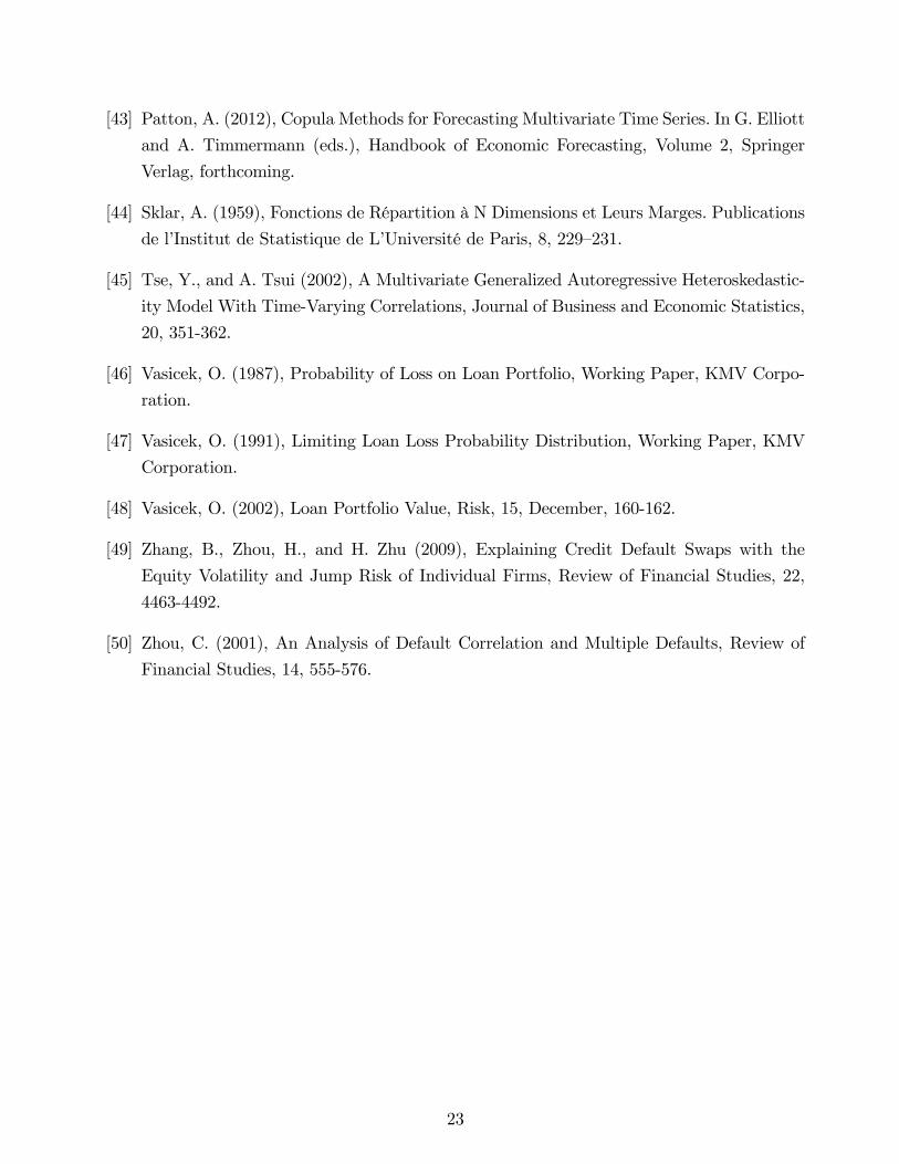
In Figure 14 we plot the CDB(50%) and V olCDB measures for CDS spreads in Panel A

and for equities in Panel B. Comparing Figures 13 and 14 (note the scales are different) we

see that the dynamic patterns are broadly similar, which is not surprising.

When comparing Panel A with Panel B in Figure 14 we see that the difference between the

CDB(50%) and V olCDB is larger for the credit portfolio than for the equity portfolio. These

results suggest that non-normality plays a large role even in a well-diversified credit portfolio,

and that relying on V olCDB would thus exaggerate the benefits from credit diversification.

Finally, in Figure 15 we analyze to which extent portfolio optimation can be employed to

avoid the decline in diversification benefits over time evident in the equal-weighted portfolio

in Figures 13-14. Each week we choose portfolio weights by maximizing CDB on a set of nine

industry portfolios each of which is equally weighted across firms in the industry. For com-

parison we also show the equal-weighted portfolio CDB from Figure 13. Figure 15 shows that

it is possible to at least partially avoid the decline in diversification benefits when optimally

rebalancing each week across industries. However, part of the decline in diversification benefits

remain. Rebalancing across individual firms may of course generate even better results but

this is computationally much more demanding as we compute the optimal portfolio weights

via simulation of the DAC model.

6 Conclusion

This paper documents cross-sectional dependence in CDS spreads, CDS-implied default in-

tensities, and equity prices. Our results are largely complementary to existing correlation

18

estimates, which typically are based on historical default rates or equity returns, and to

existing intensity-based studies, which characterize observable macro variables that induce

realistic correlation patterns in default probabilities (see Duffee (1999) and Duffi e, Saita and

Wang (2007)).

We obtain three main findings. First, copula correlations in CDS spreads and default

intensities vary substantially over our sample, with a significant increase following the financial

crisis in 2007. Equity correlations also increase in the financial crisis, but somewhat later

and the increase is less significant and not as persistent. This increase in cross-sectional

dependence is clearly important for the management of portfolio credit risk and the pricing of

structured credit products, in particular the relative pricing of CDO tranches with different

seniority levels. Second, our estimates indicate fat tails in the univariate distributions, but

also multivariate non-normalities. Multivariate asymmetries seem to be less important for

credit than they are for equities. Finally, when considering the diversification benefits from

selling credit protection, the increase in cross-sectional dependence following the financial

crisis has reduced diversification benefits, not unlike what happened in equity markets. When

computing diversification benefits, taking non-normalities into account is more important for

credit than for equity.

Our results suggest a number of extensions. First, given the richness and complexity of the

equity-implied and default intensity-implied dependence, it may prove interesting to explore

the implications for CDO valuation. In particular it would be interesting to investigate if the

resulting CDO pricing model would remove some of the observed correlation smile in CDO

tranches. See Berd, Engle, and Voronov (2007) for an example of this type of approach.

Second, an investigation of how the time-varying dependence is related to firm-specific and

economywide observables would be insightful. Third, alternative measures of credit portfolio

risk should be investigated (Vasicek 1987, 1991, 2002). Finally, we need to investigate the

robustness of the dependence patterns for default intensities when the intensities are extracted

using more sophisticated models.

19

References

[1] Ang, A., and J. Chen (2002), Asymmetric Correlations of Equity Portfolios, Journal of

Financial Economics, 63, 443-494.

[2] Berd, A., Engle, R., and A. Voronov (2007), The Underlying Dynamics of Credit Corre-

lations, Journal of Credit Risk, 3, 27-62.

[3] Berndt, A., Douglas, R., Duffi e, D., Ferguson, M., and D. Schranz (2004), Measuring

Default Risk Premia from Default Swap rates and EDFs, Working Paper, Cornell Uni-

versity.

[4] Black, F., and J. Cox, (1976), Valuing Corporate Securities: Some Effects of Bond In-

denture Provisions, Journal of Finance, 31, 351-367.

[5] Blanco, R., Brennan, S., and I. Marsh (2005), An Empirical Analysis of the Dynamic

Relationship Between Investment-Grade Bonds and Credit Default Swaps, Journal of

Finance, 60, 2255-2281.

[6] Bollerslev, T. (1986), Generalized Autoregressive Conditional Heteroskedasticity, Journal

of Econometrics, 31, 307-327.

[7] Bollerslev, T. (1990), Modelling the Coherence in Short-Run Nominal Exchange Rate:

A Multivariate Generalized ARCH Approach, Review of Economics and Statistics, 72,

498-505.

[8] Christoffersen, P., V. Errunza, K. Jacobs and H. Langlois, (2012), Is the Potential for

International Diversification Disappearing? A Dynamic Copula Approach, Review of

Financial Studies, 25, 3711-3751.

[9] Christoffersen, P. and H. Langlois, (2013), The Joint Dynamics of Equity Market Factors,

Journal of Financial and Quantitative Analysis, forthcoming.

[10] Das, R., Duffi e, D., Kapadia, N., and L. Saita (2007), Common Failings: How Corporate

Defaults are Correlated, Journal of Finance, 62, 93-117.

[11] Das, S., and R. Sundaram (2000), A Discrete-Time Approach to Arbitrage-Free Pricing

of Credit Derivatives, Management Science, 46, 46-62.

[12] Davis, M., and V. Lo (2001), Infectious Default, Quantitative Finance, 1, 382-387.

[13] deServigny, A., and O. Renault (2002), Default Correlation: Empirical Evidence, Working

Paper, Standard and Poors.

20

[14] Demarta, S., and A. J. McNeil (2004), The t Copula and Related Copulas, International

Statistical Review, 73, 111—129.

[15] Duffee, G. (1999), Estimating the Price of Default Risk, Review of Financial Studies, 12,

197-226.

[16] Duffi e, D., L. Saita and K. Wang (2007), Multi-Period Corporate Default Prediction with

Stochastic Covariates, Journal of Financial Economics, 83, 635-665.

[17] Duffi e, D., and K. Singleton (1999), Modeling Term Structures of Defaultable Bonds,

Review of Financial Studies, 12, 687-720.

[18] Duffi e, D., and K. Singleton (2003), Credit Risk, Princeton University Press.

[19] Engle, R. (1982), Autoregressive Conditional Heteroskedasticity with Estimates of the

Variance of UK Inflation, Econometrica, 50, 987-1008.

[20] Engle, R. (2002), Dynamic Conditional Correlation: A Simple Class of Multivariate

GARCH Models, Journal of Business and Economic Statistics, 20, 339-350.

[21] Engle, R., and B. Kelly (2012), Dynamic Equicorrelation, Journal of Business and Eco-

nomic Statistics, 30, 212-228.

[22] Engle, R., and K. Kroner (1995), Multivariate Simultaneous Generalized ARCH, Econo-

metric Theory, 11, 122-150.

[23] Engle, R., and J. Mezrich (1996), GARCH for Groups, Risk, 9, 36—40.

[24] Engle, R., and V. Ng. (1993), Measuring and Testing the Impact of News on Volatility,

Journal of Finance, 48, 1749—1778.

[25] Engle, R., Shephard, N., and K. Sheppard (2008), Fitting Vast Dimensional Time-Varying

Covariance Models, Working Paper, New York University.

[26] Ericsson, J., Jacobs, K., and R. Oviedo (2009), The Determinants of Credit Default Swap

Premia, Journal of Financial and Quantitative Analysis, 44, 109-132.

[27] Hansen, B. (1994), Autoregressive Conditional Density Estimation, International Eco-

nomic Review, 35, 705-730.

[28] Houweling, P., and T. Vorst (2005), Pricing Default Swaps: Empirical Evidence, Journal

of International Money and Finance, 24, 1220—1225.

21

[29] Hull, J., Predescu, M., and A. White (2006), The Valuation of Correlation-Dependent

Credit Derivatives Using a Structural Model, Working Paper, University of Toronto.

[30] Hull, J., and A. White (2000), Valuing Credit Default Swaps I: No Counter Party Default

Risk, Journal of Derivatives, 8, 29-40.

[31] Jarrow, R., Lando, D., and S. Turnbull (1997), A Markov Model for the Term Structure

of Credit Risk Spreads, Review of Financial Studies, 10, 481-523.

[32] Jarrow, R., and S. Turnbull (1995), Pricing Derivatives on Financial Securities Subject

to Credit Risk, Journal of Finance, 50, 53-85.

[33] Jarrow, R., and F. Yu (2001), Counterparty Risk and the Pricing of Defaultable Securities,

Journal of Finance, 56, 1765-1800.

[34] Jorion, P., and G. Zhang (2007), Good and Bad Credit Contagion: Evidence from Credit

Default Swaps, Journal of Financial Economics, 84, 860-881.

[35] Lando, D. (2004), Credit Risk Modeling, Princeton University Press.

[36] Leland, H. (1994), Risky Debt, Bond Covenants and Optimal Capital Structure, Journal

of Finance, 49, 1213-1252.

[37] Leland, H., and K. Toft (1996), Optimal Capital Structure, Endogenous Bankruptcy and

the Term Structure of Credit Spreads, Journal of Finance, 51, 987-1019.

[38] Longstaff, F., Mithal, S., and E. Neis (2004), Corporate Yield Spreads: Default Risk or

Liquidity? New Evidence from the Credit Default Swap Market, Journal of Finance, 60,

2213-2253.

[39] Merton, R. (1974), On the Pricing of Corporate Debt: The Risk Structure of Interest

rates, Journal of Finance, 29, 449-470.

[40] Patton, A. (2004), On the Out-of-sample Importance of Skewness and Asymmetric De-

pendence for Asset Allocation. Journal of Financial Econometrics, 2, 130—168.

[41] Patton, A. (2006A), Estimation of Multivariate Models for Time Series of Possibly Dif-

ferent Lengths, Journal of Applied Econometrics, 21, 147-173.

[42] Patton, A. (2006B), Modelling Asymmetric Exchange Rate Dependence, International

Economic Review, 47, 527—556.

22

[43] Patton, A. (2012), Copula Methods for Forecasting Multivariate Time Series. In G. Elliott

and A. Timmermann (eds.), Handbook of Economic Forecasting, Volume 2, Springer

Verlag, forthcoming.

[44] Sklar, A. (1959), Fonctions de Répartition à N Dimensions et Leurs Marges. Publications

de l’Institut de Statistique de L’Université de Paris, 8, 229—231.

[45] Tse, Y., and A. Tsui (2002), A Multivariate Generalized Autoregressive Heteroskedastic-

ity Model With Time-Varying Correlations, Journal of Business and Economic Statistics,

20, 351-362.

[46] Vasicek, O. (1987), Probability of Loss on Loan Portfolio, Working Paper, KMV Corpo-

ration.

[47] Vasicek, O. (1991), Limiting Loan Loss Probability Distribution, Working Paper, KMV

Corporation.

[48] Vasicek, O. (2002), Loan Portfolio Value, Risk, 15, December, 160-162.

[49] Zhang, B., Zhou, H., and H. Zhu (2009), Explaining Credit Default Swaps with the

Equity Volatility and Jump Risk of Individual Firms, Review of Financial Studies, 22,

4463-4492.

[50] Zhou, C. (2001), An Analysis of Default Correlation and Multiple Defaults, Review of

Financial Studies, 14, 555-576.

23

Figure 1: Weekly Median CDS Spreads, Default Intensities and Realized Equity Volatility.

2003 2005 2007 2009 20110

50

100

150

200

250

300

CDS

(bps

)

Panel A: Median CDS Spreads

2003 2005 2007 2009 20110

0.01

0.02

0.03

0.04

0.05

0.06

Def

ault

Inte

nsity

Panel B: Median Default Intensity

2003 2005 2007 2009 20110

10

20

30

40

50

60

Stoc

k Pr

ices

Panel C: Median Stock Prices

2003 2005 2007 2009 20110

20

40

60

80

100

120

140

Ann

ualiz

ed R

ealiz

edV

olat

ility

(\%

)

Panel D: Median Realized Equity Volatility

Notes to Figure: We plot the median values across the 223 equities listed in Table 1. Realized

volatility is constructed from the sum of squared daily returns during each week. The vertical

lines indicate major events during the sample period.

24

Figure 2: Interquartile Range of CDS Spreads, Default Intensities,

and Realized Equity Volatility.

2003 2005 2007 2009 20110

100

200

300

400

500

600

CDS

(bps

)

Panel A: Interquart ileRange of CDS Spreads

0

50

100

150

200

250

Num

ber of Firms

2003 2005 2007 2009 20110

0.02

0.04

0.06

0.08

0.1

0.12

Def

ault

Inte

nsity

Panel B: Interquart ileRange of Default Intensity

0

50

100

150

200

250

Num

ber of Firms

2003 2005 2007 2009 20110

20

40

60

80

Stoc

k Pr

ices

Panel C: Interquart ileRange of Stock Prices

0

50

100

150

200

250

Num

ber of Firms

Interquart ile RangeNumber of firms

2003 2005 2007 2009 20110

20

40

60

80

100

120

140

160

Ann

ualiz

ed R

ealiz

edV

olat

ility

(\%

)

Panel D: Interquart ileRange of Realized Equity Volatility

0

50

100

150

200

250

Num

ber of Firms

Notes to Figure: The grey area denote the interquartile range of the 223 equities listed in

Table 1. Realized volatility is constructed from the sum of squared daily returns during each

week. The dashes lines show the number of firms available in each sample each week.

25

Figure 3: CDS Spreads for Nine Firms.

02 05 08 110

200

400

600

800Int l Paper Co

02 05 08 110

200

400

600

800

1000

1200J C Penney

02 05 08 110

200

400

600

800Anadarko Pete Corp

02 05 08 110

100

200

300

400Allstate Corp

02 05 08 110

50

100

150

200

250Aetna Inc.

02 05 08 110

50

100

150

200

250Raytheon

02 05 08 110

50

100

150

200

250

300Hewlett Packard

02 05 08 110

200

400

600

800AT &T Corp.

02 05 08 110

50

100

150

200

250Dominion Resources Inc

Notes to Figure: We plot the CDS spreads for 9 firms in our sample, one firm for each of the

9 industries.

26

Figure 4: Median CDS Spreads and Interquartile Range for Nine Industries

02 05 08 110

200

400

600

800Basic Materials

02 05 08 110

200

400

600

800

1000

1200Consumer Goods and Services

02 05 08 110

100

200

300

400

500Energy

02 05 08 110

200

400

600

800

1000

1200Financials

02 05 08 110

50

100

150

200

250

300Healthcare

02 05 08 110

100

200

300

400

500Industrials

02 05 08 110

200

400

600

800T echnology

02 05 08 110

100

200

300

400

500

600T elecommunications Services

02 05 08 110

100

200

300

400

500Utilit ies

Notes to Figure: From the 11 industries in Markit we merge consumer goods and consumer

services. We also merge government (Freddie Mac and Fannie Mae) with financials. The

figure shows the median and interquartile range of CDS spreads within each of the remaining

9 industries.

27

Figure 5: Threshold Correlations for Weekly Log Differences:

CDS Spreads, Default Intensities and Equity Prices

­1 ­0.5 0 0.5 10

0.25

0.5Panel A: CDS Spreads

Med

ian

thre

shol

dco

rrel

atio

n

­1 ­0.5 0 0.5 10

0.25

0.5Panel B: Default Intensit ies

Med

ian

thre

shol

dco

rrel

atio

n

­1 ­0.5 0 0.5 10

0.25

0.5

Standard deviat ionsfrom the mean

Panel C: Equity Prices

Med

ian

thre

shol

dco

rrel

atio

n

Notes to Figure: For each pair of firms we compute threshold correlations on a grid of thresh-

olds defined using the standard deviation from the mean for each firm (horizontal axis). The

solid lines show the median threshold correlations across firm pairs, the grey areas mark the

interquartile ranges and the dashed lines show the threshold correlations from a bivariate

Gaussian distribution with correlation equal to the average for all the pairs of firms.

28

Figure 6: Median and Interquartile Range of Conditional Volatility:

CDS Spreads, Default Intensities, and Equity Prices

2002 2003 2004 2005 2006 2007 2008 2009 2010 2011 20120

25

50

75

100

125

150

Ann

ualiz

ed C

ondi

tiona

lV

olat

ility

(%)

Panel A: Median CDS Spread Volatility

2002 2003 2004 2005 2006 2007 2008 2009 2010 2011 20120

25

50

75

100

125

150

Ann

ualiz

ed C

ondi

tiona

lV

olat

ility

(%)

Panel B: Median Default Intensity Volat ility

2002 2003 2004 2005 2006 2007 2008 2009 2010 2011 20120

25

50

75

100

125

150

Ann

ualiz

ed C

ondi

tiona

lV

olat

ility

(%)

Panel C: Median Equity Volatility

Notes to Figure: For each firm we estimate an NGARCH model on the weekly log differ-

ences in CDS spreads, default intensities and equity prices. The plot shows the median and

interquartile range across firms of the weekly conditional volatility.

29

Figure 7: Conditional Volatility of CDS Spreads for Nine Firms.

02 05 08 110

50

100

150

200Int l Paper Co

02 05 08 110

50

100

150

200J C Penney

02 05 08 110

50

100

150

200Anadarko Pete Corp

02 05 08 110

50

100

150

200Allstate Corp

02 05 08 110

50

100

150

200Aetna Inc.

02 05 08 110

50

100

150

200Raytheon

02 05 08 110

50

100

150

200Hewlett Packard

02 05 08 110

50

100

150

200AT &T Corp.

02 05 08 110

50

100

150

200Dominion Resources Inc

Notes to Figure: We plot the conditional volatility of CDS spreads for 9 firms in our sample,

one for each industry.

30

Figure 8: Median and Interquartile Range of Conditional Volatility within Nine Industries.

02 05 08 110

50

100

150

200

250Basic Materials

02 05 08 110

50

100

150

200

250Consumer Goods and Services

02 05 08 110

50

100

150

200

250Energy

02 05 08 110

50

100

150

200

250Financials

02 05 08 110

50

100

150

200

250Healthcare

02 05 08 110

50

100

150

200

250Industrials

02 05 08 110

50

100

150

200

250T echnology

02 05 08 110

50

100

150

200

250T elecommunications Services

02 05 08 110

50

100

150

200

250Utilit ies

Notes to Figure: From the 11 industries in Markit we merge consumer goods and consumer

services. We also merge government (Freddie Mac and Fannie Mae) with financials. The figure

shows the median and interquartile range of conditional volatility of CDS spreads within each

of the remaining 9 industries.

31

Figure 9: Threshold Correlations for Weekly Residuals:

CDS Spreads, Default Intensities and Equity Prices

­1 ­0.5 0 0.5 10

0.25

0.5Panel A: CDS Spreads

Med

ian

thre

shol

dco

rrel

atio

n

­1 ­0.5 0 0.5 10

0.25

0.5Panel B: Default Intensit ies

Med

ian

thre

shol

dco

rrel

atio

n

­1 ­0.5 0 0.5 10

0.25

0.5

Standard deviat ionsfrom the mean

Panel C: Equity Prices

Med

ian

thre

shol

dco

rrel

atio

n

Notes to Figure: For each pair of firms we compute threshold correlations on the ARMA-

NGARCH residuals. The solid lines show the median threshold correlations across firm pairs,

the grey areas mark the interquartile ranges and the dashed lines show the threshold correla-

tions from a bivariate Gaussian distribution with correlation equal to the average for all the

pairs of firms.

32

Figure 10: Median and Interquartile Range of Copula Correlations:

CDS Spreads, Default Intensities and Equity Prices

2002 2003 2004 2005 2006 2007 2008 2009 2010 2011 20120

0.2

0.4

0.6

0.8Panel A: Median CDS Spread Correlat ion

Corr

elat

ion

2002 2003 2004 2005 2006 2007 2008 2009 2010 2011 20120

0.2

0.4

0.6

0.8Panel B: Medan Default Intensity Correlat ion

Corr

elat

ion

2002 2003 2004 2005 2006 2007 2008 2009 2010 2011 20120

0.2

0.4

0.6

0.8Panel C: Median Equity Correlat ion

Corr

elat

ion

Notes to Figure: Using all pairs of firms we report the median and interquartile range of the

weekly dynamic copula correlations from the DAC model.

33

Figure 11: Median and Interquartile Range of Copula Correlations for Nine Firms.

02 05 08 11­0.2

0

0.2

0.4

0.6

0.8Int l Paper Co

02 05 08 11­0.2

0

0.2

0.4

0.6

0.8J C Penney

02 05 08 11­0.2

0

0.2

0.4

0.6

0.8Anadarko Pete Corp

02 05 08 11­0.2

0

0.2

0.4

0.6

0.8Allstate Corp

02 05 08 11­0.2

0

0.2

0.4

0.6

0.8Aetna Inc.

02 05 08 11­0.2

0

0.2

0.4

0.6

0.8Raytheon

02 05 08 11­0.2

0

0.2

0.4

0.6

0.8Hewlett Packard

02 05 08 11­0.2

0

0.2

0.4

0.6

0.8AT &T Corp.

02 05 08 11­0.2

0

0.2

0.4

0.6

0.8Dominion Resources Inc

Notes to Figure: For each firm we report its median and interquartile range of correlation

with the other firms in the sample.

34

Figure 12: Median and Interquartile Range of Copula Correlations within Nine Industries

02 05 08 11

0

0.2

0.4

0.6

0.8

1Basic Materials

02 05 08 11

0

0.2

0.4

0.6

0.8

1Consumer Goods and Services

02 05 08 11

0

0.2

0.4

0.6

0.8

1Energy

02 05 08 11

0

0.2

0.4

0.6

0.8

1Financials

02 05 08 11

0

0.2

0.4

0.6

0.8

1Healthcare

02 05 08 11

0

0.2

0.4

0.6

0.8

1Industrials

02 05 08 11

0

0.2

0.4

0.6

0.8

1T echnology

02 05 08 11

0

0.2

0.4

0.6

0.8

1T elecommunications Services

02 05 08 11

0

0.2

0.4

0.6

0.8

1Utilit ies

Notes to Figure: We report the median and interquartile range of the pairwise DAC copula

correlation for all the firms in the industry with all other firms in the same industry.

35

Figure 13: Conditional Diversification Benefits.

Equal-Weighted Credit and Equity Portfolios. 5% Tail.

2004 2005 2006 2007 2008 2009 2010 2011 20120.4

0.6

0.8

1

CD

B(5

%)

Panel A: Condit ional Diversificat ion Benefit for CDS Spreads

0

20

40

60

80

VIX

Equally weightedVIX

2004 2005 2006 2007 2008 2009 2010 2011 20120.4

0.6

0.8

1

CD

B(5

%)

Panel B: Condit ional Diversificat ion Benefit for Equity Prices

0

20

40

60

80

VIX

Equally weightedVIX

Notes to Figure: Using an equal-weighted portfolio of available on-the-run CDX firms in a

given week we compute the 5% conditional diversification benefit (CDB) using our DACmodel

estimated first on CDS spreads and then on equity returns. The grey line shows the VIX on

the right-hand axis. The credit portfolio is selling credit protection by shorting CDS contracts.

36

Figure 14: Conditional Diversification Benefits.

Equal-Weighted Credit and Equity Portfolios. 50% CDB and Volatility CDB Measures.

2004 2005 2006 2007 2008 2009 2010 2011 20120.1

0.2

0.3

0.4

0.5

0.6

CD

B

Panel A: Condit ional Diversification Benefit for CDS Spreads

CDB(50%)VolCDB

2004 2005 2006 2007 2008 2009 2010 2011 20120.1

0.2

0.3

0.4

0.5

0.6

CD

B

Panel B: Condit ional Diversificat ion Benefit for Equity Prices

CDB(50%)VolCDB

Notes to Figure: Using an equal-weighted portfolio of available on-the-run CDX firms in

a given week we compute the 50% conditional diversification benefit (CDB) using our DAC

model estimated first on CDS spreads and then on equity returns. We also show the volatility-

based VolCDB measure which takes into account only volatilities and linear correlations. The

credit portfolio is selling credit protection by shorting CDS contracts.

37

Figure 15: Conditional Diversification Benefits.

Optimized Industry Weights and Equal-Weighted Credit and Equity Portfolios. 5% Tail.

2004 2005 2006 2007 2008 2009 2010 2011 20120.4

0.6

0.8

1

CDB(

5%)

Panel A: Condit ional Diversification Benefit for CDS Spreads

Equally weightedOptimized industry weights

2004 2005 2006 2007 2008 2009 2010 2011 20120.4

0.6

0.8

1

CDB(

5%)

Panel B: Condit ional Diversificat ion Benefit for Equity Prices

Equally weightedOptimized industry weights

Notes to Figure: We show the 5% CDB measure for a optimized portfolio of the 9 industry

portfolios along with an equal-weighted portfolio of individual firms. We compute the condi-

tional diversification benefit using our DAC model estimated first on CDS spreads and then

on equity returns. The grey line shows the VIX on the right-hand axis. The credit portfolio

is selling credit protection by shorting CDS contracts.

38

ACE Limited Cap One Bk USA Natl Fortune Brands, Inc. McDONALDS Corp The Kroger Co.ALLTEL Corporation Cap One Finl Corp Freeport McMoran McKesson Corporation NY Times CoAmern Elec Pwr Co Inc Cardinal Health Inc GATX Corporation MeadWestvaco Corp The TJX Companies, Inc.AT&T Corp. Caterpillar Inc. Gannett Co., Inc. MetLife, Inc. TOYS "R" US, INC.AT&T Inc. Cendant Corporation Gen Elec Cap Corp Mohawk Inds Inc Target CorporationAT&T Mobility LLC CenturyLink, Inc. General Mills, Inc. Motorola Solutions Inc Temple-Inland Inc.Aetna Inc. CenturyTel, Inc. Gen Mtrs Accep Corp Norfolk Sthn Corp Textron Finl CorpAlbertson's, Inc. Cingular Wireless LLC Goodrich Corporation Nabors Inds Inc Allstate CorpRio Tinto Alcan Inc. Cisco Systems, Inc. H. J. Heinz Company Natl Rural Utils Coop Black & Decker CorpAlcoa Inc. Ctzns Comms Co Halliburton Co Newell Rubbermaid Inc The Chubb Corporatio...Altria Group, Inc. Clear Channel Comms Inc Harrahs Oper Co Inc News America Inc Dow Chem CoAmerada Hess Corp Comcast Cable Comms LLC Hewlett Packard Co Nordstrom, Inc. The Home Depot, Inc.Amern Axle & Mfg Hldgs Comcast Corporation Hilton Hotels Corp Northrop Grumman Corp May Dept Stores CoAmern Express Co Computer Assoc Intl Inc Honeywell Intl Inc Olin Corporation Sherwin Williams CoAmern Intl Gp Inc Computer Sciences Corp IAC InterActiveCorp Omnicom Group Inc. Walt Disney CoAmgen Inc. ConAgra Foods Inc Ingersoll Rand Co Pfizer Inc. Time Warner Cable IncAnadarko Pete Corp ConocoPhillips Intelsat, Ltd. Pitney Bowes Inc. Time Warner IncArrow Electrs Inc Constellation Engy Gp Inc Intl Business Machs Progress Engy Inc Toll Bros IncAutozone Inc Ctrywde Home Lns Inc Intl Lease Fin Corp Pulte Homes, Inc. Transocean Inc.Avnet, Inc. Cox Comms Inc Intl Paper Co Quest Diagnostics Inc Tribune CompanyBarrick Gold Corp DIRECTV Holdings LLC J C Penney Co Inc R R Donnelley & Sons Tyson Foods, Inc.Bombardier Inc Darden Restaurants Inc Johnson Ctls Inc Radian Group Inc. Union Pacific Corpor...Brunswick Corp Deere & Company Jones Apparel Gp Inc RadioShack Corp United Parcel Servic...Baxter Intl Inc Dell Inc. KerrMcGee Corp Raytheon Co UnitedHealth Group I...Beam Inc. Delphi Corporation Kinder Morgan Engy Residential Cap Corp Universal Health Ser...BellSouth Corp Devon Engy Corp Knight Ridder Inc Reynolds Amern Inc Valero Energy CorpBelo Corp. Dominion Res Inc Kohls Corp Rohm & Haas Co Verizon Comms IncBerkshire Hathaway Inc Duke Energy Carolinas LLC Kraft Foods Inc. Ryder System, Inc. Verizon Global Fdg CorpBoeing Cap Corp Duke Engy Corp Lear Corporation SBC Comms Inc Viacom Inc.Bombardier Cap Inc Duke Pwr Co LLC Lennar Corporation Sears Roebuck Accep Visteon CorporationBoston Pptys Ltd E I du Pont de Nemours Liberty Media Corp SLM Corporation Vornado Realty L.P.Boston Scientific Corp EOP Oper Ltd Pship Limited Brands, Inc. Sprint Nextel Corp Wal Mart Stores IncBristol Myers Squibb Co ERP Oper Ltd Pship Liz Claiborne, Inc. SUPERVALU INC. Washington MutualBurlington Northern Eastman Chem Co Lockheed Martin Corp Sabre Holdings Corpo... Wells Fargo & CoCA, Inc. Eastman Kodak Co Loews Corporation Safeway Inc. Wendys Intl IncCdn Nat Res Ltd Electr Data Sys Corp Lowes Cos Inc Sara Lee Corporation Weyerhaeuser CoCarnival Corp Embarq Corporation M.D.C. Holdings, Inc. Sempra Energy Whirlpool CorpCBS Corporation Exelon Corporation Marriott Intl Inc Simon Ppty Gp Inc WyethCENTEX CORP Expedia, Inc. Marsh & Mclennan Cos Southwest Airls Co XL Cap LtdCIGNA Corporation Ford Mtr Cr Co MBIA Ins Corp Sprint Corporation XL Group Ltd.CIT Group Inc. Fed Home Ln Mtg Corp MBNA Corporation Staples, Inc. XLIT Ltd.CSX Corporation Fed Natl Mtg Assn Motorola Solutions Inc Starwood Hotels XTO Energy Inc.CVS Caremark Corp Fedt Dept Stores Inc Macy's, Inc. Sun Microsystems Inc Xerox CorporationCVS Corporation 1st Data Corp Masco Corporation GAP INC YUM! Brands, Inc.Campbell Soup Co FirstEnergy Corp. Maytag Corporation Hartford Financial iStar Financial Inc.Capital One Bank

Table 1: Company Names

Notes to Figure: Using data from Markit, we consider all the 226 firms included in the first 18 series of the CDX North American investment grade index dating from March 20, 2003 to September 20, 2012. We start with 226 firms and remove the 3 firms (in bold italics) which do not have a consecutive 52-week history.

Average Standard Deviation Skewness Kurtosis

CDS SpreadsMedian 0.01 0.01 1.62 6.44Interquartile Range [0.01, 0.02] [0.00, 0.01] [1.09, 2.35] [3.92, 9.69]

Default IntensitiesMedian 0.02 0.01 1.65 6.51Interquartile Range [0.01, 0.03] [0.01, 0.02] [1.09, 2.34] [3.92, 9.34]

Equity PricesMedian 32.71 9.28 0.14 2.47Interquartile Range [23.89, 45.37] [6.17, 13.82] [-0.19, 0.59] [2.02, 3.18]

Annualized Average (%)

Annualized Standard

Deviation (%)Skewness Kurtosis Jarque-Bera p-

valueAR(1)

CoefficientAR(2)

Coefficient

CDS SpreadsMedian 3.25 66.97 0.81 10.23 0.00 0.08 0.05Interquartile Range [-23.13, 12.84] [52.58, 73.39] [-0.87, 1.44] [5.02, 15.23] [0.00, 0.00] [-0.05, 0.13] [-0.06, 0.09]

Default IntensitiesMedian 3.28 67.82 0.74 10.12 0.00 0.08 0.05Interquartile Range [-23.85, 12.89] [53.39, 74.49] [-0.72, 1.37] [5.05, 14.96] [0.00, 0.00] [-0.05, 0.12] [-0.05, 0.08]

Equity PricesMedian 3.25 34.02 -0.47 7.40 0.00 -0.04 -0.02Interquartile Range [-20.78, 8.08] [21.00, 42.28] [-2.51, -0.15] [4.31, 10.94] [0.00, 0.00] [-0.15, 0.01] [-0.10, 0.03]

CDS Spreads Default Intensities

Equity Prices

CDS SpreadsMedian 0.37 0.99 -0.32Interquartile Range [0.12, 0.46] [0.97, 0.99] [-0.50, -0.25]

Default IntensitiesMedian 0.39 -0.32Interquartile Range [0.12, 0.47] [-0.50, -0.25]

Equity PricesMedian 0.32Interquartile Range [0.15, 0.42]

Table 2: Descriptive Statistics on CDS Spreads, Default Intensities and Equity Prices

Panel B: Sample Moments on Weekly Log-Differences

Panel A: Sample Moments on Weekly Levels

Panel C: Correlations of Weekly Log-Differences

Notes to Table: We report sample moments on weekly CDS spreads, default intensities and equity prices across available firms. Panel A computes the moments for spreads, intensities and prices in levels. Panel B reports sample moments computed on the weekly log-differences. Panel C reports average sample correlations across firms using weekly log-differences. On the diagonal we report the median and IQR across the correlations between each firm and all other firms. On the off-diagonal we report the median and IQR of the correlation between different series for the same firm.

Proportion of Model Chosen by AICC Criterion CDS Spreads Default Intensities Equity PricesARMA(0,0) 10% 12% 6%ARMA(0,1) 10% 8% 7%ARMA(0,2) 9% 12% 10%ARMA(1,0) 14% 17% 5%ARMA(1,1) 14% 11% 7%ARMA(1,2) 4% 4% 8%ARMA(2,0) 11% 12% 9%ARMA(2,1) 7% 5% 11%ARMA(2,2) 20% 19% 37%

Parameter Estimates µ Median 0.0004 0.0005 0.0004

Interquartile Range [-0.0006, 0.0022] [-0.0007, 0.0023] [-0.0005, 0.0017]AR(1) Median 0.099 0.091 -0.018

Interquartile Range [-0.185, 0.594] [-0.181, 0.560] [-0.816, 0.472]AR(2) Median -0.142 -0.337 -0.621

Interquartile Range [-0.772, 0.097] [-0.843, 0.088] [-0.833, -0.101]MA(1) Median 0.072 0.080 -0.032

Interquartile Range [-0.519, 0.353] [-0.514, 0.300] [-0.507, 0.776]MA(2) Median 0.449 0.362 0.597

Interquartile Range [0.100, 0.894] [0.087, 0.917] [0.059, 0.847]L-B(4) p-value > 5% Proportion 99% 99% 96%

Parameter Estimates CDS Spreads Default Intensities Equity Pricesω Median 0.0003 0.0005 0.0000

Interquartile Range [0.0002, 0.0010] [0.0002, 0.0010] [0.0000, 0.0001]β Median 0.769 0.760 0.794

Interquartile Range [0.635, 0.844] [0.641, 0.843] [0.703, 0.855]α Median 0.139 0.136 0.048

Interquartile Range [0.094, 0.203] [0.088, 0.198] [0.027, 0.084]γ Median -0.168 -0.211 1.313

Interquartile Range [-0.431, 0.028] [-0.479, -0.028] [0.819, 2.263]Volatility Persistence Median 0.954 0.941 0.978

Interquartile Range [0.894, 0.980] [0.894, 0.977] [0.961, 0.990]ν Median 3.604 3.653 6.549

Interquartile Range [3.166, 4.159] [3.232, 4.305] [5.117, 8.425]λ Median 0.076 0.067 -0.109

Interquartile Range [0.042, 0.121] [0.025, 0.107] [-0.159, -0.061]L-B(4) p-value z2 > 5% Proportion 98% 97% 92%

Table 3: Summary of ARMA-NGARCH Estimation on Weekly Log-Differences

Panel A: Conditional Mean Dynamics

Panel B: Conditional Volatility Dynamics and Return Distribution

Notes to Table: For each firm we estimate an ARMA(p,q)-NGARCH(1,1) model where the p and q are chosen by the AICC criterion. The residual distribution is asymmetric t with parameters ν and λ. L-B(4) denotes a Ljung-Box test that the residuals (Panel A) or squared residuals (Panel B) are serially uncorrelated.

Skewness Kurtosis

CDS Spreads Median 0.88 9.84Interquartile Range [0.40, 1.67] [6.60, 20.37]

Default Intensities Median 0.84 9.18Interquartile Range [0.37, 1.49] [6.30, 18.37]

Equity Prices Median -0.45 5.23Interquartile Range [-0.74, -0.22] [4.25, 7.15]

CDS Spreads Default Intensities Equity Prices

CDS Spreads Median 0.33 0.98 -0.30Interquartile Range [0.23, 0.42] [0.97, 0.98] [-0.37, -0.20]

Default Intensities Median 0.34 -0.29Interquartile Range [0.25, 0.43] [-0.36, -0.20]

Equity Prices Median 0.29Interquartile Range [0.23, 0.37]

Panel A: Sample Moments

Panel B: Correlation Between CDS, Default Intensity and Equity

Notes to Table: Using the ARMA-NGARCH residuals, z, we compute the skewness, kurtosis and cross-correlation and report the median and interquartile range across firms in Panel A. We also compute for each firm the correlation between CDS spreads, default intensities and equity residuals and report the median and interquartile range in Panel B. On the diagonal we report the median and IQR across the correlations between each firm and all other firms. On the off-diagonal we report the median and IQR of the correlation between different series for the same firm.

Table 4: Descriptive Statistics of Model Residuals

CDS Spreads Default Intensities Equity PricesβC 0.958 0.956 0.930αC 0.021 0.024 0.019Correlation Persistence 0.980 0.980 0.949νC 13.572 13.548 13.354λC 0.048 0.045 - 0.380Composite Log-likelihood 1,074,513 1,167,893 617,594

CDS Spreads Default Intensities Equity PricesβC 0.960 0.960 0.930αC 0.021 0.022 0.019Correlation Persistence 0.982 0.983 0.949νC 13.590 12.888 13.217Composite Log-likelihood 1,073,786 1,167,612 604,583

CDS Spreads Default Intensities Equity PricesβC 0.960 0.960 0.924αC 0.020 0.021 0.018Correlation Persistence 0.981 0.981 0.942Composite Log-likelihood 1,025,863 1,115,747 573,347

Notes to Table: We estimate the dynamic asymmetric copula (DAC), the dynamic symmetric copula (DSC), and the dynamic normal copula (DNC) models on the 223 firms in our sample. Each of the three models is estimated on each of our three data sets containing ARMA-NGARCH residuals from weekly log-differences on CDS spreads, default intensities and equity prices.

Table 5: Dynamic Copula Parameter Estimation

Panel C: Dynamic Normal Copula Estimation

Panel B: Dynamic Symmetric Copula Estimation

Panel A: Dynamic Asymmetric Copula Estimation