Embed Size (px)
Citation preview
Dynamic Factor Models and FactorAugmented Vector Autoregressions
Lawrence J. Christiano
Dynamic Factor Models and FactorAugmented Vector Autoregressions
• Problem:— the time series dimension of data is relatively short.— the number of time series variables is huge.
• DFM’s and FAVARs take the position:— there are many variables and, hence, shocks,— but, the principle driving force of all the variables may be justa small number of shocks.
• Factor view has a long-standing history in macro.— almost the definition of macroeconomics: a handfull of shocks- demand, supply, etc. - are the principle economic drivers.
— Sargent and Sims: only two shocks can explain a large fractionof the variance of US macroeconomic data.• 1977, “Business Cycle Modeling Without Pretending to HaveToo Much A-Priori Economic Theory,” in New Methods inBusiness Cycle Research, ed. by C. Sims et al., Minneapolis:Federal Reserve Bank of Minneapolis.
Why Work with a Lot of Data?
• Estimates of impulse responses to, say, a monetary policyshock, may be distorted by not having enough data in theanalysis (Bernanke, et. al. (QJE, 2005))
— Price puzzle:• measures of inflation tend to show transitory rise to a monetarypolicy tightening shock in standard (small-sized) VARs.
• One interpretation: Monetary authority responds to a signalabout future inflation that is captured in data not included in astandard, small-sized VAR.
• May suppose that ‘core inflation’is a factor that can only bededuced from a large number of different data.
• May want to know (as in Sargent and Sims), whether the datafor one country or a collection of countries can be characterizedas the dynamic response to a few factors.
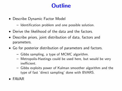
Outline
• Describe Dynamic Factor Model— Identification problem and one possible solution.
• Derive the likelihood of the data and the factors.• Describe priors, joint distribution of data, factors andparameters.
• Go for posterior distribution of parameters and factors.— Gibbs sampling, a type of MCMC algorithm.— Metropolis-Hastings could be used here, but would be veryineffi cient.
— Gibbs exploits power of Kalman smoother algorithm and thetype of fast ‘direct sampling’done with BVARS.
• FAVAR
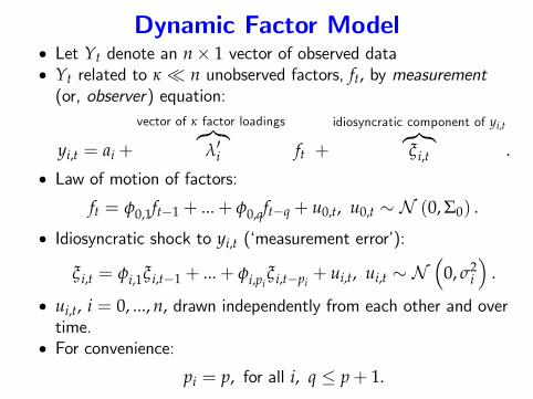
Dynamic Factor Model• Let Yt denote an n× 1 vector of observed data• Yt related to κ � n unobserved factors, ft, by measurement(or, observer) equation:
yi,t = ai +
vector of κ factor loadings︷︸︸︷λ′i ft +
idiosyncratic component of yi,t︷︸︸︷ξi,t .
• Law of motion of factors:
ft = φ0,1ft−1 + ...+ φ0,qft−q + u0,t, u0,t ∼ N (0, Σ0) .
• Idiosyncratic shock to yi,t (‘measurement error’):
ξi,t = φi,1ξ i,t−1 + ...+ φi,piξ i,t−pi
+ ui,t, ui,t ∼ N(
0, σ2i
).
• ui,t, i = 0, ..., n, drawn independently from each other and overtime.
• For convenience:
pi = p, for all i, q ≤ p+ 1.
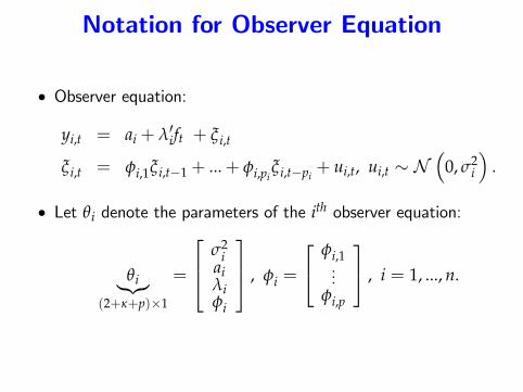
Notation for Observer Equation
• Observer equation:
yi,t = ai + λ′ift + ξi,t
ξi,t = φi,1ξ i,t−1 + ...+ φi,piξi,t−pi
+ ui,t, ui,t ∼ N(
0, σ2i
).
• Let θi denote the parameters of the ith observer equation:
θi︸︷︷︸(2+κ+p)×1
=
σ2i
aiλiφi
, φi =
φi,1...
φi,p
, i = 1, ..., n.
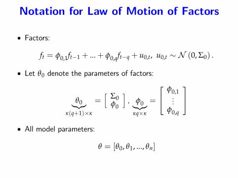
Notation for Law of Motion of Factors
• Factors:
ft = φ0,1ft−1 + ...+ φ0,qft−q + u0,t, u0,t ∼ N (0, Σ0) .
• Let θ0 denote the parameters of factors:
θ0︸︷︷︸κ(q+1)×κ
=[ Σ0
φ0
], φ0︸︷︷︸
κq×κ
=
φ0,1...
φ0,q
• All model parameters:
θ = [θ0, θ1, ..., θn]
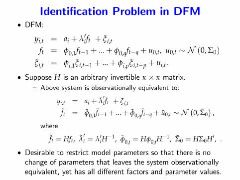
Identification Problem in DFM• DFM:
yi,t = ai + λ′ift + ξi,t
ft = φ0,1ft−1 + ...+ φ0,qft−q + u0,t, u0,t ∼ N (0, Σ0)
ξi,t = φi,1ξi,t−1 + ...+ φi,pξi,t−p + ui,t.
• Suppose H is an arbitrary invertible κ × κ matrix.— Above system is observationally equivalent to:
yi,t = ai + λ′i ft + ξ i,t
ft = φ0,1 ft−1 + ...+ φ0,q ft−q + u0,t ∼ N(0, Σ0
),
where
ft = Hft, λ′i = λ′iH
−1, φ0,j = Hφ0,jH−1, Σ0 = HΣ0H′, .
• Desirable to restrict model parameters so that there is nochange of parameters that leaves the system observationallyequivalent, yet has all different factors and parameter values.
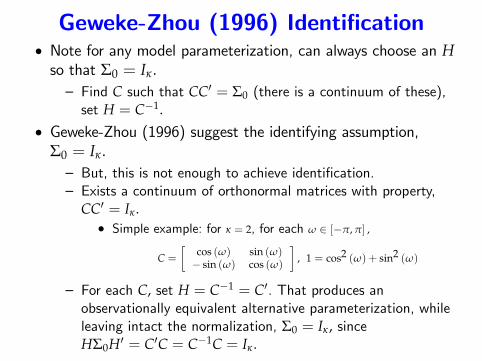
Geweke-Zhou (1996) Identification• Note for any model parameterization, can always choose an Hso that Σ0 = Iκ.— Find C such that CC′ = Σ0 (there is a continuum of these),set H = C−1.
• Geweke-Zhou (1996) suggest the identifying assumption,Σ0 = Iκ.— But, this is not enough to achieve identification.— Exists a continuum of orthonormal matrices with property,
CC′ = Iκ.• Simple example: for κ = 2, for each ω ∈ [−π, π] ,
C =[
cos (ω) sin (ω)− sin (ω) cos (ω)
], 1 = cos2 (ω) + sin2 (ω)
— For each C, set H = C−1 = C′. That produces anobservationally equivalent alternative parameterization, whileleaving intact the normalization, Σ0 = Iκ, sinceHΣ0H′ = C′C = C−1C = Iκ.
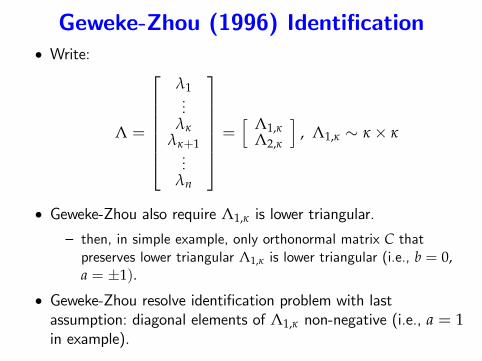
Geweke-Zhou (1996) Identification• Write:
Λ =
λ1...
λκλκ+1...
λn
=[ Λ1,κ
Λ2,κ
], Λ1,κ ∼ κ × κ
• Geweke-Zhou also require Λ1,κ is lower triangular.
— then, in simple example, only orthonormal matrix C thatpreserves lower triangular Λ1,κ is lower triangular (i.e., b = 0,a = ±1).
• Geweke-Zhou resolve identification problem with lastassumption: diagonal elements of Λ1,κ non-negative (i.e., a = 1in example).
Geweke-Zhou (1996) Identification
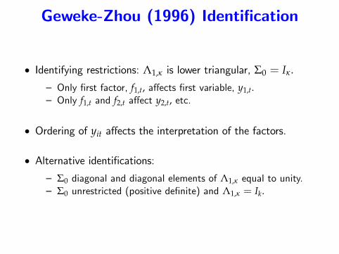
• Identifying restrictions: Λ1,κ is lower triangular, Σ0 = Iκ.
— Only first factor, f1,t, affects first variable, y1,t.— Only f1,t and f2,t affect y2,t, etc.
• Ordering of yit affects the interpretation of the factors.
• Alternative identifications:— Σ0 diagonal and diagonal elements of Λ1,κ equal to unity.— Σ0 unrestricted (positive definite) and Λ1,κ = Ik.
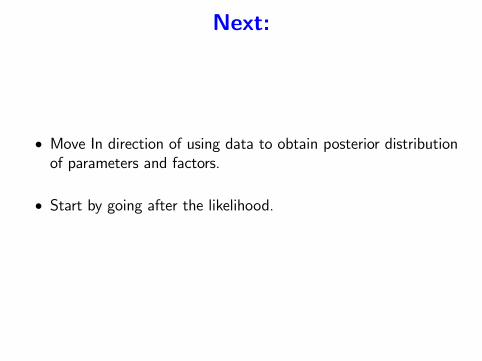
Next:
• Move In direction of using data to obtain posterior distributionof parameters and factors.
• Start by going after the likelihood.
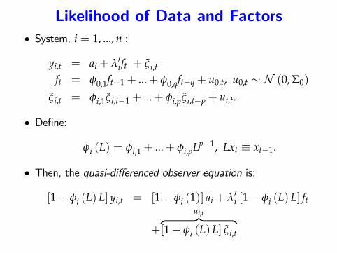
Likelihood of Data and Factors• System, i = 1, ..., n :
yi,t = ai + λ′ift + ξi,t
ft = φ0,1ft−1 + ...+ φ0,qft−q + u0,t, u0,t ∼ N (0, Σ0)
ξi,t = φi,1ξi,t−1 + ...+ φi,pξi,t−p + ui,t.
• Define:
φi (L) = φi,1 + ...+ φi,pLp−1, Lxt ≡ xt−1.
• Then, the quasi-differenced observer equation is:
[1− φi (L) L] yi,t = [1− φi (1)] ai + λ′i [1− φi (L) L] ft
+
ui,t︷ ︸︸ ︷[1− φi (L) L] ξi,t
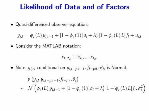
Likelihood of Data and of Factors
• Quasi-differenced observer equation:
yi,t = φi (L) yi,t−1 + [1− φi (1)] ai + λ′i [1− φi (L) L] ft + ui,t
• Consider the MATLAB notation:
xt1:t2 ≡ xtt , ..., xt2 .
• Note: yi,t, conditional on yi,t−p:t−1, ft−p:t, θi, is Normal:
p(yi,t|yi,t−p:t−1, ft−p:t, θi
)∼ N
(φi (L) yi,t−1 + [1− φi (1)] ai + λ′i [1− φi (L) L] ft, σ2
i
)
Likelihood of Data and of Factors
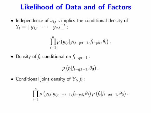
• Independence of ui,t’s implies the conditional density ofYt = [ y1,t · · · yn,t ]
′ :
n
∏i=1
p(yi,t|yi,t−p:t−1, ft−p:t, θi
).
• Density of ft conditional on ft−q:t−1 :
p(ft|ft−q:t−1, θ0
).
• Conditional joint density of Yt, ft :
n
∏i=1
p(yi,t|yi,t−p:t−1, ft−p:t, θi
)p(ft|ft−q:t−1, θ0
).
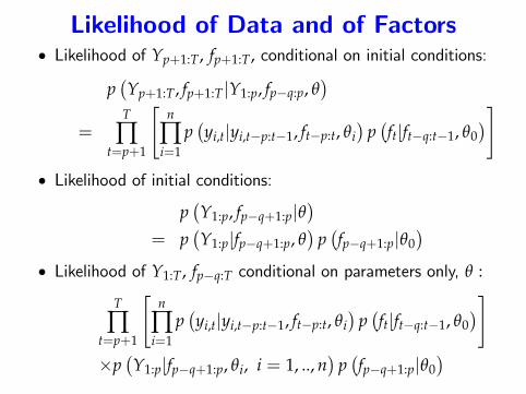
Likelihood of Data and of Factors• Likelihood of Yp+1:T, fp+1:T, conditional on initial conditions:
p(Yp+1:T, fp+1:T|Y1:p, fp−q:p, θ
)=
T
∏t=p+1
[n
∏i=1
p(yi,t|yi,t−p:t−1, ft−p:t, θi
)p(ft|ft−q:t−1, θ0
)]• Likelihood of initial conditions:
p(Y1:p, fp−q+1:p|θ
)= p
(Y1:p|fp−q+1:p, θ
)p(fp−q+1:p|θ0
)• Likelihood of Y1:T, fp−q:T conditional on parameters only, θ :
T
∏t=p+1
[n
∏i=1
p(yi,t|yi,t−p:t−1, ft−p:t, θi
)p(ft|ft−q:t−1, θ0
)]×p(Y1:p|fp−q+1:p, θi, i = 1, .., n
)p(fp−q+1:p|θ0
)
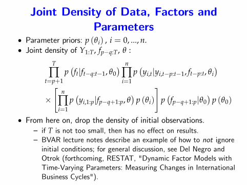
Joint Density of Data, Factors andParameters
• Parameter priors: p (θi) , i = 0, ..., n.• Joint density of Y1:T, fp−q:T, θ :
T
∏t=p+1
p(ft|ft−q:t−1, θ0
) n
∏i=1
p(yi,t|yi,t−p:t−1, ft−p:t, θi
)×[
n
∏i=1
p(yi,1:p|fp−q+1:p, θ
)p (θi)
]p(fp−q+1:p|θ0
)p (θ0)
• From here on, drop the density of initial observations.— if T is not too small, then has no effect on results.— BVAR lecture notes describe an example of how to not ignoreinitial conditions; for general discussion, see Del Negro andOtrok (forthcoming, RESTAT, "Dynamic Factor Models withTime-Varying Parameters: Measuring Changes in InternationalBusiness Cycles").
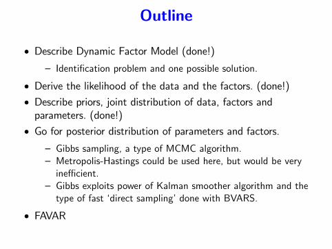
Outline
• Describe Dynamic Factor Model (done!)— Identification problem and one possible solution.
• Derive the likelihood of the data and the factors. (done!)• Describe priors, joint distribution of data, factors andparameters. (done!)
• Go for posterior distribution of parameters and factors.— Gibbs sampling, a type of MCMC algorithm.— Metropolis-Hastings could be used here, but would be veryineffi cient.
— Gibbs exploits power of Kalman smoother algorithm and thetype of fast ‘direct sampling’done with BVARS.
• FAVAR
Gibbs Sampling
• Idea is similar to what we did with the Metropolis-Hastingsalgorithm.
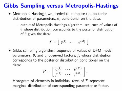
Gibbs Sampling versus Metropolis-Hastings• Metropolis-Hastings: we needed to compute the posteriordistribution of parameters, θ, conditional on the data.
— output of Metropolis-Hastings algorithm: sequence of values ofθ whose distribution corresponds to the posterior distributionof θ given the data:
P =[
θ(1) · · · θ(M)]
• Gibbs sampling algorithm: sequence of values of DFM modelparameters, θ, and unobserved factors, f , whose distributioncorresponds to the posterior distribution conditional on thedata:
P =[
θ(1) · · · θ(M)
f (1) · · · f (M)
].
Histogram of elements in individual rows of P representmarginal distribution of corresponding parameter or factor.
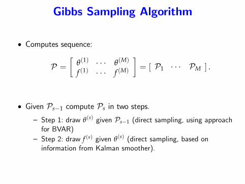
Gibbs Sampling Algorithm
• Computes sequence:
P =[
θ(1) · · · θ(M)
f (1) · · · f (M)
]= [ P1 · · · PM ] .
• Given Ps−1 compute Ps in two steps.
— Step 1: draw θ(s) given Ps−1 (direct sampling, using approachfor BVAR)
— Step 2: draw f (s) given θ(s) (direct sampling, based oninformation from Kalman smoother).
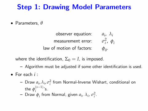
Step 1: Drawing Model Parameters
• Parameters, θ
observer equation: ai, λi
measurement error: σ2i , φi
law of motion of factors: φ0.
where the identification, Σ0 = I, is imposed.— Algorithm must be adjusted if some other identification is used.
• For each i :
— Draw ai, λi, σ2i from Normal-Inverse Wishart, conditional on
the φ(s−1)i ’s.
— Draw φi from Normal, given ai, λi, σ2i .
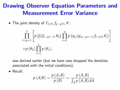
Drawing Observer Equation Parameters andMeasurement Error Variance
• The joint density of Y1:T, fp−q:T, θ :
T
∏t=p+1
[p(ft|ft−q:t−1, θ0
) n
∏i=1
p(yi,t|yi,t−p:t−1, ft−p:t, θi
)]
×p (θ0)n
∏i=1
p (θi) ,
was derived earlier (but we have now dropped the densitiesassociated with the initial conditions).
• Recall,
p (A|B) = p (A, B)p (B)
=p (A, B)∫
A p (A, B) dA
Drawing Observer Equation Parameters andMeasurement Error Variance
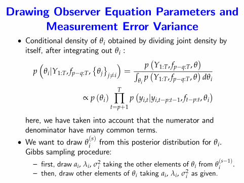
• Conditional density of θi obtained by dividing joint density byitself, after integrating out θi :
p(
θi|Y1:T, fp−q:T,{
θj}
j 6=i
)=
p(Y1:T, fp−q:T, θ
)∫θi
p(Y1:T, fp−q:T, θ
)dθi
∝ p (θi)T
∏t=p+1
p(yi,t|yi,t−p:t−1, ft−p:t, θi
)here, we have taken into account that the numerator anddenominator have many common terms.
• We want to draw θ(s)i from this posterior distribution for θi.
Gibbs sampling procedure:
— first, draw ai, λi, σ2i taking the other elements of θi from θ
(s−1)i .
— then, draw other elements of θi taking ai, λi, σ2i as given.
Drawing Observer Equation Parameters andMeasurement Error Variance
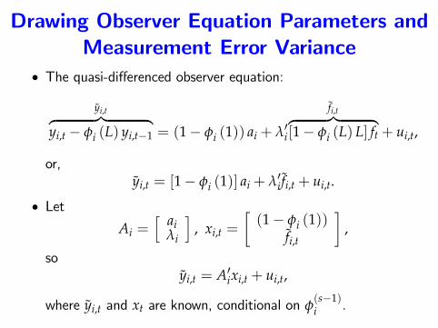
• The quasi-differenced observer equation:
yi,t︷ ︸︸ ︷yi,t − φi (L) yi,t−1 = (1− φi (1)) ai + λ′i
fi,t︷ ︸︸ ︷[1− φi (L) L] ft + ui,t,
or,yi,t = [1− φi (1)] ai + λ′i fi,t + ui,t.
• LetAi =
[ aiλi
], xi,t =
[(1− φi (1))
fi,t
],
soyi,t = A′ixi,t + ui,t,
where yi,t and xt are known, conditional on φ(s−1)i .
Drawing Observer Equation Parameters andMeasurement Error Variance
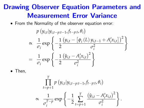
• From the Normality of the observer equation error:
p(yi,t|yi,t−p:t−1, ft−p:t, θi
)∝
1σi
exp
{−1
2
(yi,t −
[φi (L) yi,t−1 +A′ixi,t
])2
σ2i
}
=1σi
exp
{−1
2
(yi,t −A′ixi,t
)2
σ2i
}• Then,
T
∏t=p+1
p(yi,t|yi,t−p:t−1, ft−p:t, θi
)∝
1
σT−pi
exp
{−1
2
T
∑t=p+1
(yi,t −A′ixi,t
)2
σ2i
}.
Drawing Observer Equation Parameters andMeasurement Error Variance
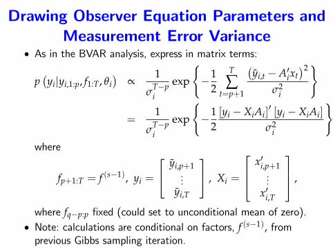
• As in the BVAR analysis, express in matrix terms:
p(yi|yi,1:p, f1:T, θi
)∝
1
σT−pi
exp
{−1
2
T
∑t=p+1
(yi,t −A′ixt
)2
σ2i
}
=1
σT−pi
exp
{−1
2[yi −XiAi]
′ [yi −XiAi]
σ2i
},
where
fp+1:T = f (s−1), yi =
yi,p+1...
yi,T
, Xi =
x′i,p+1...
x′i,T
,
where fq−p:p fixed (could set to unconditional mean of zero).• Note: calculations are conditional on factors, f (s−1), fromprevious Gibbs sampling iteration.
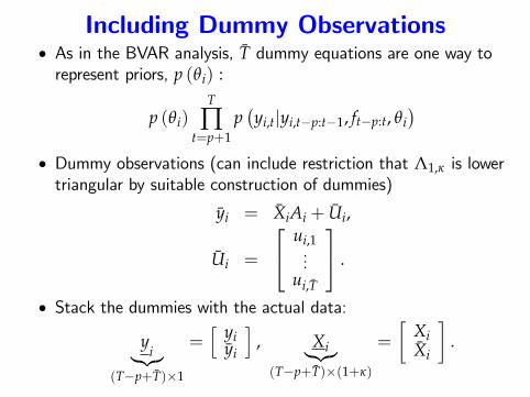
Including Dummy Observations• As in the BVAR analysis, T dummy equations are one way torepresent priors, p (θi) :
p (θi)T
∏t=p+1
p(yi,t|yi,t−p:t−1, ft−p:t, θi
)• Dummy observations (can include restriction that Λ1,κ is lowertriangular by suitable construction of dummies)
yi = XiAi + Ui,
Ui =
ui,1...
ui,T
.
• Stack the dummies with the actual data:
yi︸︷︷︸
(T−p+T)×1
=[ yi
yi
], Xi︸︷︷︸(T−p+T)×(1+κ)
=
[XiXi
].
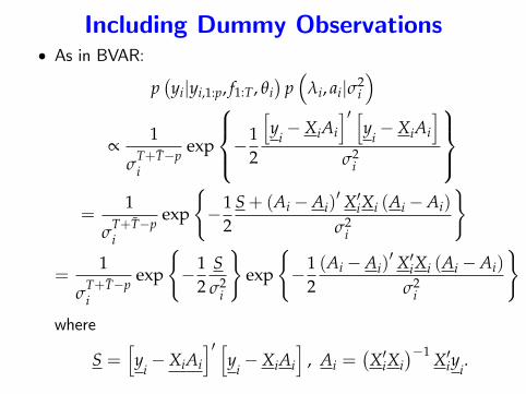
Including Dummy Observations• As in BVAR:
p(yi|yi,1:p, f1:T, θi
)p(
λi, ai|σ2i
)∝
1
σT+T−pi
exp
−12
[y
i−XiAi
]′ [y
i−XiAi
]σ2
i
=
1
σT+T−pi
exp
{−1
2S+ (Ai −Ai)
′ X′iXi (Ai −Ai)
σ2i
}
=1
σT+T−pi
exp
{−1
2Sσ2
i
}exp
{−1
2(Ai −Ai)
′ X′iXi (Ai −Ai)
σ2i
}where
S =[y
i−XiAi
]′ [y
i−XiAi
], Ai =
(X′iXi
)−1 X′iyi.
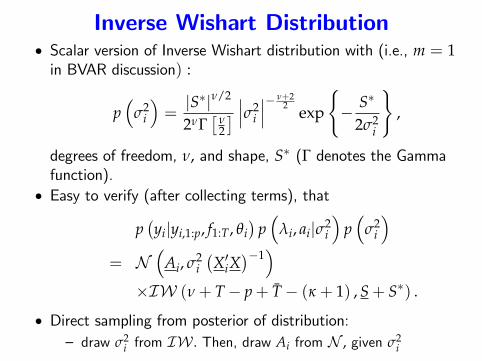
Inverse Wishart Distribution• Scalar version of Inverse Wishart distribution with (i.e., m = 1in BVAR discussion) :
p(
σ2i
)=|S∗|ν/2
2νΓ[
ν2
] ∣∣∣σ2i
∣∣∣− ν+22 exp
{− S∗
2σ2i
},
degrees of freedom, ν, and shape, S∗ (Γ denotes the Gammafunction).
• Easy to verify (after collecting terms), that
p(yi|yi,1:p, f1:T, θi
)p(
λi, ai|σ2i
)p(
σ2i
)= N
(Ai, σ2
i(X′iX
)−1)
×IW (ν+ T− p+ T− (κ + 1) , S+ S∗) .
• Direct sampling from posterior of distribution:— draw σ2
i from IW . Then, draw Ai from N , given σ2i
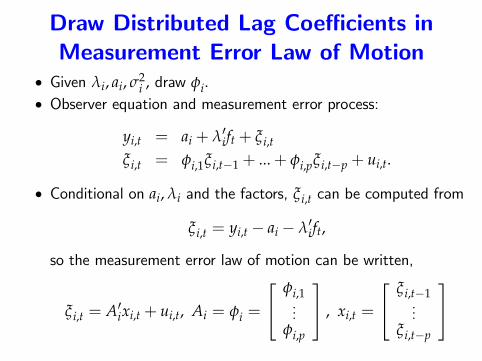
Draw Distributed Lag Coeffi cients inMeasurement Error Law of Motion
• Given λi, ai, σ2i , draw φi.
• Observer equation and measurement error process:
yi,t = ai + λ′ift + ξi,t
ξi,t = φi,1ξi,t−1 + ...+ φi,pξi,t−p + ui,t.
• Conditional on ai, λi and the factors, ξi,t can be computed from
ξi,t = yi,t − ai − λ′ift,
so the measurement error law of motion can be written,
ξi,t = A′ixi,t + ui,t, Ai = φi =
φi,1...
φi,p
, xi,t =
ξi,t−1...
ξi,t−p
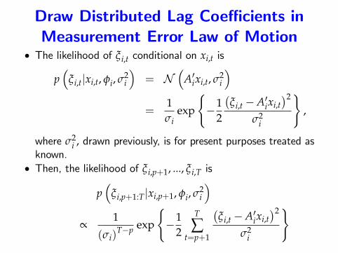
Draw Distributed Lag Coeffi cients inMeasurement Error Law of Motion
• The likelihood of ξi,t conditional on xi,t is
p(
ξi,t|xi,t, φi, σ2i
)= N
(A′ixi,t, σ2
i
)=
1σi
exp
{−1
2
(ξi,t −A′ixi,t
)2
σ2i
},
where σ2i , drawn previously, is for present purposes treated as
known.• Then, the likelihood of ξi,p+1, ..., ξi,T is
p(
ξi,p+1:T|xi,p+1, φi, σ2i
)∝
1
(σi)T−p exp
{−1
2
T
∑t=p+1
(ξi,t −A′ixi,t
)2
σ2i
}
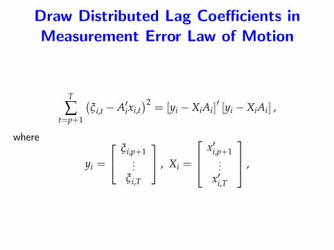
Draw Distributed Lag Coeffi cients inMeasurement Error Law of Motion
T
∑t=p+1
(ξi,t −A′ixi,t
)2= [yi −XiAi]
′ [yi −XiAi] ,
where
yi =
ξi,p+1...
ξi,T
, Xi =
x′i,p+1...
x′i,T
,
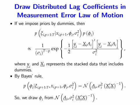
Draw Distributed Lag Coeffi cients inMeasurement Error Law of Motion
• If we impose priors by dummies, then
p(
ξi,p+1:T|xi,p+1, φi, σ2i
)p (φi)
∝1
(σi)T−p exp
−12
[y
i−XiAi
]′ [y
i−XiAi
]σ2
i
,
where yiand Xi represents the stacked data that includes
dummies.• By Bayes’rule,
p(
φi|ξi,p+1:T, xi,p+1, φi, σ2i
)= N
(Ai, σ2
i(X′iX
)−1)
.
So, we draw φi from N(
Ai, σ2i(X′iX
)−1)
.
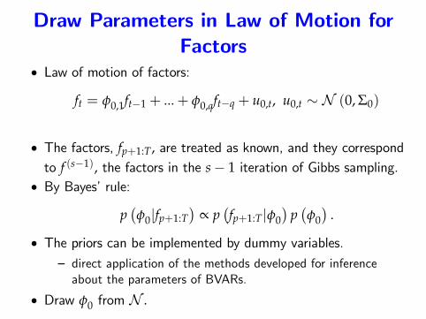
Draw Parameters in Law of Motion forFactors
• Law of motion of factors:
ft = φ0,1ft−1 + ...+ φ0,qft−q + u0,t, u0,t ∼ N (0, Σ0)
• The factors, fp+1:T, are treated as known, and they correspondto f (s−1), the factors in the s− 1 iteration of Gibbs sampling.
• By Bayes’rule:
p(φ0|fp+1:T
)∝ p
(fp+1:T|φ0
)p(φ0)
.
• The priors can be implemented by dummy variables.— direct application of the methods developed for inferenceabout the parameters of BVARs.
• Draw φ0 from N .
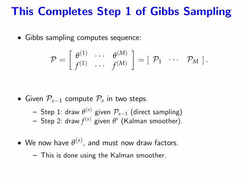
This Completes Step 1 of Gibbs Sampling
• Gibbs sampling computes sequence:
P =[
θ(1) · · · θ(M)
f (1) · · · f (M)
]= [ P1 · · · PM ] .
• Given Ps−1 compute Ps in two steps.
— Step 1: draw θ(s) given Ps−1 (direct sampling)— Step 2: draw f (s) given θs (Kalman smoother).
• We now have θ(s), and must now draw factors.
— This is done using the Kalman smoother.
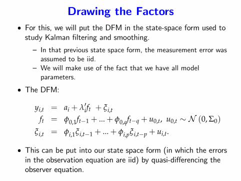
Drawing the Factors• For this, we will put the DFM in the state-space form used tostudy Kalman filtering and smoothing.
— In that previous state space form, the measurement error wasassumed to be iid.
— We will make use of the fact that we have all modelparameters.
• The DFM:
yi,t = ai + λ′ift + ξi,t
ft = φ0,1ft−1 + ...+ φ0,qft−q + u0,t, u0,t ∼ N (0, Σ0)
ξi,t = φi,1ξi,t−1 + ...+ φi,pξi,t−p + ui,t.
• This can be put into our state space form (in which the errorsin the observation equation are iid) by quasi-differencing theobserver equation.
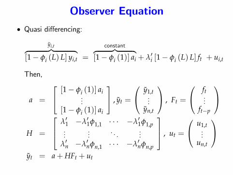
Observer Equation• Quasi differencing:
yi,t︷ ︸︸ ︷[1− φi (L) L] yi,t =
constant︷ ︸︸ ︷[1− φi (1)] ai + λ′i [1− φi (L) L] ft + ui,t
Then,
a =
[1− φi (1)] ai...
[1− φi (1)] ai
, yt =
y1,t...
yn,t
, Ft =
ft...
ft−p
H =
λ′1 −λ′1φ1,1 · · · −λ′1φ1,p...
.... . .
...λ′n −λ′nφn,1 · · · −λ′nφn,p
, ut =
u1,t...
un,t
yt = a+HFt + ut
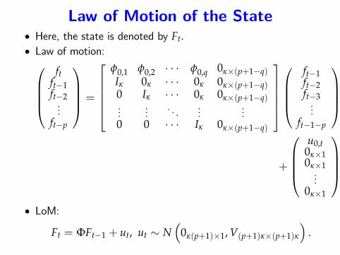
Law of Motion of the State• Here, the state is denoted by Ft.• Law of motion:
ftft−1ft−2...
ft−p
=
φ0,1 φ0,2 · · · φ0,q 0κ×(p+1−q)Iκ 0κ · · · 0κ 0κ×(p+1−q)0 Iκ · · · 0κ 0κ×(p+1−q)...
.... . .
......
0 0 · · · Iκ 0κ×(p+1−q)
ft−1ft−2ft−3...
ft−1−p
+
u0,t
0κ×10κ×1...
0κ×1
• LoM:
Ft = ΦFt−1 + ut, ut ∼ N(
0κ(p+1)×1, V(p+1)κ×(p+1)κ
).
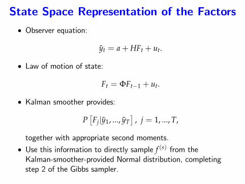
State Space Representation of the Factors• Observer equation:
yt = a+HFt + ut.
• Law of motion of state:
Ft = ΦFt−1 + ut.
• Kalman smoother provides:
P[Fj|y1, ..., yT
], j = 1, ..., T,
together with appropriate second moments.• Use this information to directly sample f (s) from theKalman-smoother-provided Normal distribution, completingstep 2 of the Gibbs sampler.
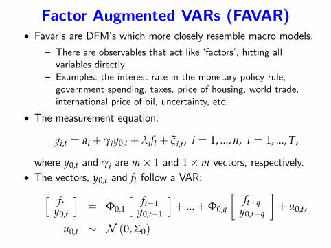
Factor Augmented VARs (FAVAR)• Favar’s are DFM’s which more closely resemble macro models.
— There are observables that act like ‘factors’, hitting allvariables directly
— Examples: the interest rate in the monetary policy rule,government spending, taxes, price of housing, world trade,international price of oil, uncertainty, etc.
• The measurement equation:
yi,t = ai + γiy0,t + λift + ξ i,t, i = 1, ..., n, t = 1, ..., T,
where y0,t and γi are m× 1 and 1×m vectors, respectively.• The vectors, y0,t and ft follow a VAR:[ ft
y0,t
]= Φ0,1
[ ft−1y0,t−1
]+ ...+Φ0,q
[ft−q
y0,t−q
]+ u0,t,
u0,t ∼ N (0, Σ0)
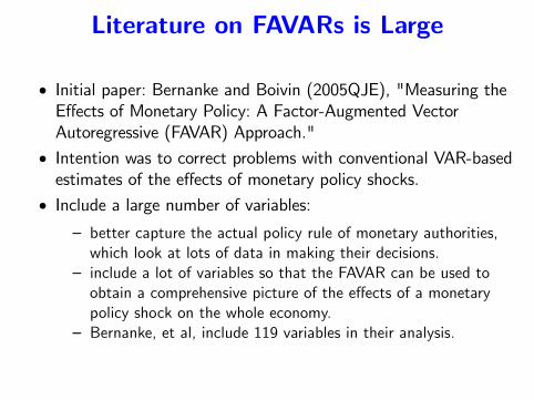
Literature on FAVARs is Large
• Initial paper: Bernanke and Boivin (2005QJE), "Measuring theEffects of Monetary Policy: A Factor-Augmented VectorAutoregressive (FAVAR) Approach."
• Intention was to correct problems with conventional VAR-basedestimates of the effects of monetary policy shocks.
• Include a large number of variables:— better capture the actual policy rule of monetary authorities,which look at lots of data in making their decisions.
— include a lot of variables so that the FAVAR can be used toobtain a comprehensive picture of the effects of a monetarypolicy shock on the whole economy.
— Bernanke, et al, include 119 variables in their analysis.
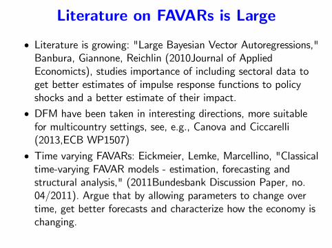
Literature on FAVARs is Large
• Literature is growing: "Large Bayesian Vector Autoregressions,"Banbura, Giannone, Reichlin (2010Journal of AppliedEconomicts), studies importance of including sectoral data toget better estimates of impulse response functions to policyshocks and a better estimate of their impact.
• DFM have been taken in interesting directions, more suitablefor multicountry settings, see, e.g., Canova and Ciccarelli(2013,ECB WP1507)
• Time varying FAVARs: Eickmeier, Lemke, Marcellino, "Classicaltime-varying FAVAR models - estimation, forecasting andstructural analysis," (2011Bundesbank Discussion Paper, no.04/2011). Argue that by allowing parameters to change overtime, get better forecasts and characterize how the economy ischanging.


![· Web viewR-codes C = vector aanmaken Bv. Leeftijd leeftijd [1] 18 22 17 19 19 Factor = getallen in vector zijn niet numeriek, hierdoor weet R dat](https://img.pdfslide.net/doc/110x75/5e62d344cdf1f635c7726492/web-view-r-codes-c-vector-aanmaken-bv-leeftijd-leeftijd-1-18-22-17-19-19-factor.jpg)