Embed Size (px)
Citation preview

Dynamic Interbank Network Analysis Using Latent Space Models
Fernando Linardi, Cees Diks, Marco van der Leij and Iuri Lazier
November 2018
487

ISSN 1518-3548 CGC 00.038.166/0001-05
Working Paper Series Brasília no. 487 Novemberr 2018 p. 1-46

Working Paper Series
Edited by the Research Department (Depep) – E-mail: [email protected]
Editor: Francisco Marcos Rodrigues Figueiredo – E-mail: [email protected]
Co-editor: José Valentim Machado Vicente – E-mail: [email protected]
Head of the Research Department: André Minella – E-mail: [email protected]
The Banco Central do Brasil Working Papers are all evaluated in double-blind refereeing process.
Reproduction is permitted only if source is stated as follows: Working Paper no. 487.
Authorized by Carlos Viana de Carvalho, Deputy Governor for Economic Policy.
General Control of Publications
Banco Central do Brasil
Comun/Divip
SBS – Quadra 3 – Bloco B – Edifício-Sede – 2º subsolo
Caixa Postal 8.670
70074-900 Brasília – DF – Brazil
Phones: +55 (61) 3414-3710 and 3414-3565
Fax: +55 (61) 3414-1898
E-mail: [email protected]
The views expressed in this work are those of the authors and do not necessarily reflect those of the Banco Central do
Brasil or its members.
Although the working papers often represent preliminary work, citation of source is required when used or reproduced.
As opiniões expressas neste trabalho são exclusivamente do(s) autor(es) e não refletem, necessariamente, a visão do Banco Central do Brasil.
Ainda que este artigo represente trabalho preliminar, é requerida a citação da fonte, mesmo quando reproduzido parcialmente.
Citizen Service Division
Banco Central do Brasil
Deati/Diate
SBS – Quadra 3 – Bloco B – Edifício-Sede – 2º subsolo
70074-900 Brasília – DF – Brazil
Toll Free: 0800 9792345
Fax: +55 (61) 3414-2553
Internet: http//www.bcb.gov.br/?CONTACTUS

Non-technical Summary
Since financial institutions are highly interconnected, network theory provides a
useful framework for the analysis of the financial system. In this paper, we present
a model to handle dynamic network data based on the latent space approach. The
dynamic network data consist of a set of banks (nodes) and a set of links which represent
the existence of lending or borrowing operations between banks observed over one year.
The latent space refers to a space of unobserved characteristics of banks that affect
link formation. The model assumes that each node has a position in this latent space
and the closer two nodes are, the more likely they will form a link. Estimation of
the positions of banks in the latent space and other parameters of the model are done
within a Bayesian framework.
We apply this methodology to analyze two different datasets: the unsecured in-
terbank network and the repo (secured) interbank network. We include in the model
variables that measure characteristics of the banks to investigate how they affect the
probability of a lending connection between banks. We also compare the goodness-of-fit
of the latent space model and the model without such structure. In the second model,
the probability of a link between banks depends only on observed variables, such as
their size and volume of credit and deposits.
Our main results show that the model which incorporates observed bank’s char-
acteristics and a latent space is able to capture some features of the network data such
as transitivity. We show that the inclusion of a latent space is essential to account for
dependencies that exist among banks. Furthermore, the distribution of graph statistics
for the model with a latent space is much closer to the observed values when compared
to the model without a latent space. We show that the model without the latent space,
in which the probability of forming a tie depends only on observed characteristics of
banks, has a poor fit. Therefore, models that do not incorporate dependencies in the
analysis of network data will suffer from misspecification which may lead to invalid
conclusions.
3

Sumario Nao Tecnico
Como as instituicoes financeiras estao altamente interligadas, a teoria de rede
fornece um arcabouco util para a analise do sistema financeiro. Neste artigo, apresen-
tamos um modelo para lidar com dados dinamicos de redes com base na abordagem
do espaco latente. Os dados dinamicos consistem em um conjunto de bancos (nos)
e um conjuto de links, que representam a existencia de operacoes de emprestimo en-
tre os bancos observadas durante um ano. O espaco latente refere-se a um espaco de
caracterısticas nao observaveis dos bancos que afetam a formacao dos links. O mod-
elo pressupoe que cada no tem uma posicao neste espaco latente e quanto menor e a
distancia entre os nos, maior a probabilidade que eles formem um link. As posicoes dos
bancos no espaco latente e outros parametros do modelo sao estimados utilizando uma
abordagem bayesiana.
Nos utilizamos essa metodologia para analisar dois conjuntos de dados difer-
entes: as redes de emprestimos interbancarias sem garantia e as com garantia de tıtulos
publicos (operacoes compromissadas). Nos incluımos no modelo variaveis que medem
as caracterısticas de bancos com o objetivo de investigar como elas afetam a proba-
bilidade de conexao entre dois bancos. Comparamos tambem o ajuste do modelo de
espaco latente e o modelo sem tal estrutura. No segundo modelo, a probabilidade
de uma conexao entre bancos depende apenas de caracterısticas observadas como o
tamanho e os volumes de credito e depositos das instituicoes.
Nosso principal resultado mostra que o modelo que incorpora as caracterısticas
do banco e o espaco latente e capaz de capturar algumas caracterısticas dos dados,
como transitividade. Mostramos que a inclusao de um espaco latente e essencial para
explicar as dependencias que existem entre os bancos. Alem disso, a distribuicao das
estatısticas de rede para o modelo que incluı o espaco latente esta mais proxima dos
valores observados quando comparada ao modelo sem o espaco latente. Nos mostramos
que o modelo sem o espaco latente, que depende apenas das caracterısticas observadas
dos bancos, tem um ajuste ruim. Portanto, modelos que nao incorporam dependencias
na analise de dados da rede sofrem de erros de especificacao, o que pode invalidar as
conclusoes.
4

Dynamic Interbank Network Analysis Using Latent
Space Models
Fernando Linardi1
Cees Diks2
Marco van der Leij3
Iuri Lazier4
Abstract
Longitudinal network data are increasingly available, allowing researchers to
model how networks evolve over time and to make inference on their dependence
structure. In this paper, a dynamic latent space approach is used to model di-
rected networks of monthly interbank exposures. In this model, each node has an
unobserved temporal trajectory in a low-dimensional Euclidean space. Model pa-
rameters and latent banks’ positions are estimated within a Bayesian framework.
We apply this methodology to analyze two different datasets: the unsecured and
the secured (repo) interbank lending networks. We show that the model that
incorporates a latent space performs much better than the model in which the
probability of a tie depends only on observed characteristics; the latent space
model is able to capture some features of the dyadic data, such as transitivity,
that the model without a latent space is not able to.
Keywords: network dynamics, latent position model, interbank network, Bayesian
inference.
JEL Classification: C11, D85, G21
The Working Papers should not be reported as representing the views of the Banco
Central do Brasil. The views expressed in the papers are those of the authors and
do not necessarily reflect those of the Banco Central do Brasil.
1University of Amsterdam and Central Bank of Brazil. e-mail: [email protected], University of Amsterdam and Tinbergen Institute. e-mail: [email protected], University of Amsterdam, Tinbergen Institute and Research Department, De Neder-
landsche Bank. e-mail: [email protected] Bank of Brazil. e-mail: [email protected]
5

1 Introduction
There has been a growing interest in the study of networks in economics over the last
years. Specifically in finance the accelerated loss of confidence in financial markets
following the failure of Lehman Brothers in 2008 has shown the importance of under-
standing the network of linkages between financial institutions. The lack of knowledge
of counterparty exposures and how the contagion would spread throughout the system
during the crisis have led policy makers to adopt a large set of financial reforms to
address these and other vulnerabilities, both at the international and domestic levels
(Claessens and Kodres, 2014).
Since financial institutions are highly interconnected, network theory provides a
useful framework for the analysis of the financial system. Interconnections may be
directed due to banks’ claims on each other or may arise indirectly when banks hold
similar portfolios or share a common pool of investors or depositors. The role of these
interconnections in the propagation of shocks in financial networks has been analyzed
by a growing literature. Allen and Gale (2000) and Freixas et al. (2000) have shown how
contagion depends on the structure of the interbank network. In a more recent work,
Acemoglu et al. (2015) show that for a small shock hitting the system a more connected
financial network enhances financial stability. On the other hand, a less connected
financial network is preferable in the case of a large shock since interconnections serve
as a mechanism for shock propagation. Many other theoretical or simulation-based
works have studied the relevance of the various possible channels of contagion in the
propagation of shocks and the implications for financial stability1. The work in this area
usually corroborates the “robust-yet-fragile” tendency of financial systems described by
Gai and Kapadia (2010), in which the probability of contagion may be low but, when
problems occur, the effects can be widespread
1See Huser (2015) and Glasserman and Young (2016) for recent reviews of the extensive literatureon channels of contagion in financial networks.
6

The statistical challenge in analyzing network data is to describe the potential
dependence among nodes. For instance, in social network data the probability of a tie
between two individuals increases as the characteristics of them become more similar
(homophily). Equally important is the individual level heterogeneity, reflected in differ-
ences in observed characteristics, which plays an important role in the creation of new
links. However, a main concern is the unobserved heterogeneity (see, e.g., Fafchamps
et al., 2010).
In this paper, we present a model to handle dynamic network data with directed
binary edges based on the latent space approach2. The model was originally introduced
by Hoff et al. (2002) for static networks and later extended by Krivitsky et al. (2009) to
account for clustering and homophily which is often observed in network data. Then,
Sarkar and Moore (2005), Durante and Dunson (2014) and Sewell and Chen (2015)
have proposed latent space models for dynamic networks.
In this model, the latent space refers to a space of unobserved characteristics
that affect link formation. The model assumes that the presence of a link between two
banks is independent of all other links in the system, given the unobserved positions in
the latent space and observed characteristics of the nodes. Each node has a position
in this low dimensional Euclidean space and the closer two nodes are, the more likely
they will form a link. Although the interdependence between dyads is not explicitly
parameterized, in the latent space model they are represented by latent variables. For
this reason, the model can account for higher-order dependencies, such as reciprocity
and transitivity, which are usually present in network data. So, the observation of ties
i → j and j → k suggests that the nodes i, j and k are not too far apart making the
existence of ties j → i (reciprocity) and i→ k (transitivity) more probable. Estimation
2The “latent space” has been used in economics to account for the unobserved homophily thatmight affect the formation and behavior of social networks (Goldsmith-Pinkham and Imbens, 2013and Graham, 2014). Iijima and Kamada (2017) develop a network formation model in which thebenefit and the cost of link formation depend on the social distance between agents.
7

of the latent positions and the parameters of the model is done within a Bayesian
framework.
A contribution of the paper is to use the dynamic latent space approach of Sewell
and Chen (2015) to model monthly networks of directed interbank linkages. The la-
tent space model has been mostly used for modeling social networks but it has not
been applied to the study of financial networks so far. Although financial exposures
are naturally represented by a weighted network, the choice of using a directed net-
work representation is motivated by our aim to evaluate the ability of the model to
characterize the basic structure of the network, which is the presence or absence of a
link.
In this dynamic model each node has a temporal trajectory in the latent space.
Hence, we expect to have a better understanding of how the network evolves over
time and the behavior of individual banks instead of conducting separate analyses for
each network or averaging graph statistics. We extended the model to include in the
observation equation covariates that measures characteristics of the pair of banks and
we are able to investigate how these pair-specific measures such as size, liquidity, etc.,
affect the probability of forming a lending connection.
The motivation to use a dynamic network model is that papers usually consider the
network structure of banks’ exposures as fixed. They do not consider strategic actions
that other banks may take to reduce the exposure to a bank in distress or liquidity
hoarding in moments of increased uncertainty about the health of the financial system.
For example, Afonso et al. (2011) examine the impact of the financial crisis of 2008 on
the US interbank market and show how banks have become more restrictive in their
lending operations after the Lehman Brothers’ bankruptcy. Squartini et al. (2013)
show the changes in the topology of the Dutch interbank network over the period
1998-2008. Despite the importance of contributions, a limited number of empirical
papers explore the dynamics of financial networks. Most of them measure certain graph
8

statistics over time instead of modeling the network dynamics in order to understand
the changes in the network topology (Giraitis et al., 2016)3. The reason for this is the
greater complexity in modeling dynamic network data given the dependence structures
of networks observed over discrete time intervals. Further motivation to use a dynamic
network model is that currently central bank authorities collect a huge amount of
data on bilateral exposures of financial institutions or they are able to derive them
from payment system records4. Using the increasing availability of longitudinal data,
researchers can model how the network evolves over time to make inference on its
dependence structure.
We apply this methodology to analyze two different datasets: the unsecured and
the secured interbank lending networks. We analyze these two networks separately
since banks face distinct risks when lending in these markets. In unsecured lending,
loans are not collateralised so lenders are directly exposed to losses in the case of
borrowers default. In secured lending, which in our case is represented by repurchase
agreements (repo) collateralized with government bonds, the loss is limited by the
collateral value. In the former, counterparty risk plays a key role (see, e.g., Afonso
et al., 2011) while in the latter the quality of collateral is an issue in moments of distress
(see, e.g., Krishnamurthy et al., 2014). Despite the differences in risk assessment, graph
statistics of the two networks are quite similar.
We estimate the model with the latent space but an important question is whether
it improves the model’s goodness-of-fit. The latent space is expected to account for the
unobserved bank attributes that affect the link formation and improve the model’s fit.
Hence, we run a model in which the probability of a tie depends only on observed
covariates xijt and a second one in which the latent space is included. The former
3For instance, Craig and von Peter (2014) track the number and composition of banks in the coreand periphery on a quarterly basis as an evidence of tiering in the German banking system. They usethe blockmodeling approach.
4The algorithms to extract the information from large value payment systems are usually based onthe work of Furfine (1999) and later refinements.
9

model is simply a logistic regression model in which directed ties are the dependent
variables. We assess the in-sample and the out-of-sample link predictions of the two
models. In addition, we evaluate the adequacy of them by comparing some selected
graph statistics calculated for the observed data with their distributions obtained from
a large number of networks simulated according to the fitted model (see, e.g., Hunter
et al., 2008; Durante et al., 2017). If the simulated network does not resemble the
observed network for a particular statistic, it is an indication of the model’s lack of
fit. We use this procedure to assess the model’s fit considering a set of graph statistics
which are believed to represent important structural properties of interbank networks
such as degree distribution, reciprocity and assortativity.
Our main results show that the model which incorporates observed bank’s char-
acteristics and a latent space to account for the unobserved ones is able to capture
some features of the dyadic data such as transitivity. We show that the inclusion of a
low dimensional latent space is essential to account for dependencies that exist among
nodes. Further, the distribution of graph statistics for the simulated networks based on
the model with a latent space are much closer to the observed values when compared
to the model without a latent space. On the other hand, the model in which the proba-
bility of forming a tie depends only on observed characteristics of banks has a poor fit.
Link predictions are much worse and the distribution of most graph statistics for the
simulated networks are far from the observed values. Therefore, models that do not in-
corporate dependencies in the analysis of network data will suffer from misspecification
which may lead to invalid conclusions.
Lastly, the latent space approach is related to other statistical models for the anal-
ysis of network data. The methodology for dynamic network analysis is less developed
since most of the models are for modeling static networks5. However, given the impor-
5Some models are intended for static networks but the processes for link creation or modificationare dynamic. Examples are the Erdos-Renyi random graphs, preferential attachment and small-worldmodels. See Goldenberg et al. (2009) for a survey of static and dynamic network models.
10

tance of the subject, statistical models for the analysis of longitudinal network data are
emerging. Examples of dynamic network models are the stochastic actor-based model
(Snijders and Steglich, 2015) and the extension of the Exponential Random Graph
Model (ERGM) for modeling dynamic networks (Hanneke et al., 2010). The former
assumes that the objective function depends on preferences for certain types of social
structures, such as reciprocated dyads or transitive triads, while the latter depends
on counts of specific network structures such as edges, triangles, k-stars, etc. Other
methodology related to the latent space approach is the mixed membership stochastic
blockmodel (Xing et al., 2010) which allows each node to belong to multiple blocks
with fractional membership. In general, the models assume a continuous or a discrete
Markov process to represent the network dynamics. However, the first two modeling ap-
proaches assume a homogeneous representation of the network behavior, while the last
ones allow for nodal heterogeneity in model parameters. Finally, a different approach
combines agent-based modeling and the literature on strategic network formation to
gain some economic intuition on the network formation process. Banks’ utility func-
tions are defined at the start and network formation follows a game theoretical approach
(see e.g. Blasques et al., 2015).
The rest of the paper is organized as follows. Section 2 describes the latent space
model for dynamic networks. Section 3 provides an explanation of the Bayesian es-
timation of model parameters. Section 4 describes the data on unsecured interbank
exposures, repo transactions and bank variables. In Section 5 we analyze the two dy-
namic networks and report the main results and in Section 6 we discuss the importance
of the latent space. Finally, in Section 7 we present a brief conclusion.
11
2 The model
In this section we describe the dynamic latent space approach of Sewell and Chen (2015)
for modeling the interbank network. The borrowing and lending relationships of the
interbank market can be represented by a graph Gt = (N , Et) where N is the set of all
nodes and Et is the set of edges at time t ∈ T = {1, 2, ..., T}. The number of nodes
which represent financial institutions is n = |N |. It will be assumed that Et consists of
directed edges representing whether or not a lending or a borrowing relationship exists
between two banks at time t.
Each node i has an unobserved position in a p-dimensional Euclidean latent space
Rp. Let zit represent the p-dimensional vector of the ith node’s latent position at time t
and Zt is the n× p matrix whose ith row is zit. The n× n square matrix Yt = {yijt} is
the adjacency matrix of the directed network observed at time t where yijt = 1 if bank
i has a credit exposure to bank j at time t and 0 otherwise. There are also a vector
xijt and a n× n× d array Xt of observed characteristics of the dyads.
It is assumed that the latent node positions follow a Markov process. It is also
assumed that the observed graph at time t is conditionally independent of all other
graphs, given the latent positions and dyadic-level covariate information at time t.
These assumptions lead to the representation of the temporal series of graphs as a state
space model given in terms of densities by:
Yt ∼ f (Yt|Zt,Xt,β) (1)
Zt ∼ g (Zt|Zt−1,ψ) (2)
for t = 1, 2, . . . , T , where ψ and β are sets of model parameters. Equation (1) is the
observation equation that relates the observed graphs Yt to the latent state variable
Zt representing the positions of nodes in a low dimensional Euclidean space. Equation
12

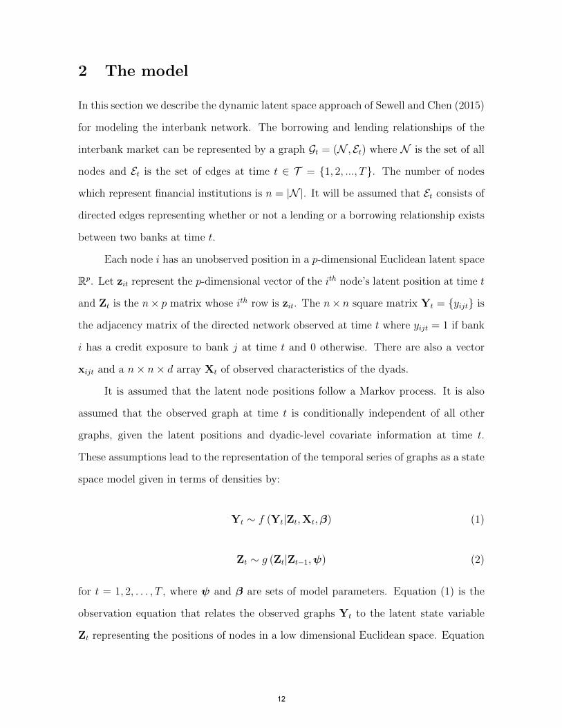
Figure 1: Graphical representation the Markovian dependencies between states Zt and observationsYt.
(2) is the state transition equation that governs the time evolution of the unobserved
latent state. A graphical representation of the dependencies between different states
and observations is shown in Figure 1.
Xing et al. (2010) and Sewell and Chen (2015) assume that the evolution of the
latent node positions follows a random walk. They show that even this simple model
provides a better representation of the data than a static model that ignores time
dependence between networks. Therefore, the initial distribution of the latent node
positions and transition equation for t = 2, 3, ..., T are given by
π(Z1|ψ) =n∏i=1
MVNp(zi1|0, τ 2Ip) (3)
π(Zt|Zt−1,ψ) =n∏i=1
MVNp(zit|zi(t−1), σ2Ip), (4)
where Ip is the p × p identity matrix, MVNp(z|µ,Σ) denotes the p-dimensional mul-
tivariate normal probability density function with mean µ and covariance matrix Σ
13

evaluated at z.
The logistic regression model is a convenient parameterization for the link prob-
ability (Hoff et al., 2002). The authors take a conditional independence approach to
modeling by assuming that the probability of a link between two nodes is conditionally
independent of all other links, given the latent positions and the observed characteristics
of the dyad:
P(yijt = 1|zit, zjt,xijt,β) =exp(yijtηijt)
1 + exp(ηijt). (5)
In general, the logit6 of the link probability in latent space models is written as
a linear function of covariates and a function of the distance of latent positions. Using
the original parameterization of Hoff et al. (2002) for the dynamic network case, we
have:
ηijt = logit(P(yijt = 1|·)) = β0 + β′xijt − dijt, (6)
where the constant controls the overall density of the network, β is a vector of unknown
parameters, xijt is a d -length vector of dyad specific covariates and dijt =‖ zit − zjt ‖
is the Euclidean distance between nodes i and j within the latent space at time t. Hoff
et al. (2002) call this formulation the distance model.
The distance model (equation 6) has a simple interpretation. The likelihood of
a tie between i and j is a function of banks’ observed and unobserved characteristics
that might affect network formation. Examples of observed bank characteristics can be
asset size, deposits or available liquidity. Unobserved latent characteristics can be, for
example, private information about counterparty risk or the existence of a relationship
between two banks in other markets which affects the probability of a link in the
observed network. In this setting, the latent space can be interpreted as a characteristic
space where banks that are closer together have a higher probability of forming lending
or borrowing relationships. Banks’ positions in this space can help identify groups of
6logit(p) = log(p/(1-p)).
14

banks that are similar to each other in terms of lending and borrowing behavior, after
controlling for the explanatory variables.
In equation 6 we included only observed variables of the pair of banks and their
positions in latent space to account for the unobserved characteristics that affect link
formation. As we show in Sections 4 and 5 the links between banks are quite stable over
the period of analysis, and macroeconomic variables such as GDP growth do not seem
to affect the link formation process. One explanation could be the different frequency
of observation of the variables. The networks are based on monthly data that are end-
of-month exposures or aggregation of daily data; to capture the effect of low frequency
data on the formation of links we may need to analyze longer periods.
Finally, the likelihood of the conditional independence model is:
P(Y1:T |Z1:T ,X1:T ,β) =T∏t=1
∏i6=j
P(yijt|zit, zjt,xijt,β) =T∏t=1
∏i6=j
exp(yijtηijt)
1 + exp(ηijt). (7)
3 Estimation
A Bayesian approach is used to obtain estimates of the latent space positions and of
the unknown parameters simultaneously. The posterior distribution
π (Z1:T ,ψ,β|Y1:T ,X1:T ) , (8)
where ψ = (τ 2, σ2), is sampled using the Metropolis-Hastings algorithm within Gibbs
sampling.
One problem of the model is that the likelihood is a function of the latent posi-
tions only through their distances. However, the distance is invariant under reflection,
rotation and translation of the latent positions and, consequently, for each n × p ma-
trix of latent positions Zt there is an infinite number of other positions given the same
15

log-likelihood, i.e., log P(Yt|Zt, ...) = log P(Yt|Z∗t , ...) for any Z∗t that is equivalent to
Zt under the operations of reflection, rotation and translation.
To resolve the problem of the non-uniqueness of the estimates, Hoff et al. (2002)
perform a Procrustean transformation on Zt. The goal is to transform a given matrix
to be as close as possible to the target matrix by any combination of reflection, rotation
and translation7. First, we choose the initial latent positions to be the (nd)× T target
matrix Z0. Then, after each iteration of the MCMC algorithm the coordinates of Z =
(Z′1, ...,Z
′T )
′are transformed to be as close as possible to the corresponding coordinates
of Z0. The transformation does not change the distances nor the likelihood but it
approximately fixes the location of Z and makes MCMC iterations comparable.
We use standard prior distributions and the values of the prior hyperparame-
ters are set to make the priors weakly informative. The prior distributions for the
parameters are set as follows: τ 2 ∼ IG(ντ/2, ντξ2τ/2), σ2 ∼ IG(νσ/2, νσξ
2σ/2) and
β ∼ MVN(µβ,Σβ), where IG and MVN are the inverse gamma and the multivari-
ate normal distributions, respectively. The inverse gamma distribution was chosen as
it is a conjugate prior for the unknown parameters τ 2 and σ2.
The values of prior hyperparameters (ντ , ξ2τ , νσ, ξ
2σ,µβ,Σβ) are set based on the
suggestions of Sewell and Chen (2015). In general, we use relatively diffuse prior dis-
tributions. The shape and scale parameters for τ 2 were set to low values in order to
have a weakly informative prior. The same procedure was used for σ2. In addition, the
value of ξ2τ was set to be equal to the initial estimate of τ 2 (equation 19). The prior
for β has zero mean and large variance. Nonetheless, we found that the estimation is
robust to changes in the values of prior hyperparameters and the convergence of the
parameters is not affect.
7Formally, the Procrustean transformation of Z using Z0 as the target matrix solves the problem:
argminT Z tr(Z0 − T Z)′(Z0 − T Z)
where T is a set of reflections, rotations and translations.
16

3.1 Posterior sampling and the MCMC algorithm
We implement a Markov Chain Monte Carlo (MCMC) algorithm to sample from the
posterior to obtain estimates of the latent positions and other unknown parameters
of the model8. The model parameters τ 2 and σ2 are sampled directly from their full
conditional distributions using the Gibbs sampler while conditional distributions which
do not have closed forms are sampled using a standard Metropolis-Hastings (MH) al-
gorithm. The conditional distributions used in the MH steps are given in Appendix A
where we derive in detail the conditional distribution of Zt as well as the conditional
distributions of the latent position zit and parameters (τ 2, σ2,β).
In order to reduce the time for the Markov chain to get to stationarity, we seek
reasonable estimates for the initial values of the latent positions Z1:T and the parameters
τ 2, σ2, and β. The procedure to obtain the starting values is detailed in Appendix B.
Given the starting values of Z1:T , τ 2, σ2 and β and current values at scan s of the
Markov chain, the MH algorithm generates a new set of parameter values as follows:
1. For t = 1, ..., T and for i = 1, ..., n, sample z(s+1)it using a MH step with a normal
random walk proposal distribution.
2. Sample β(s+1) using a MH step with a multivariate normal random walk proposal
distribution.
3. Sample τ 2(s+1) from its full conditional distribution.
4. Sample σ2(s+1) from its full conditional distribution.
Finally, the variance of the proposal distributions are tuned automatically to
achieve acceptance rates of 35% based on the algorithm proposed by Haario et al.
(2005).
8The algorithm is based on the R codes of Sewell and Chen (2015).
17

4 Data
The Central Bank of Brazil collects and processes data of exposures between financial
institutions from different sources as credit register, securities custody and settlement
systems and derivatives central counterparties. The dataset built by the central bank
includes exposures of banks, credit unions, securities dealers and other financial insti-
tutions.
We restrict our analyses to exposures between approximately 135 banking institu-
tions, from a total universe of over 1,500 banking and non-banking financial institutions.
This sample does not lose relevance, since non-banking financial institutions account
for only 2.7% of the financial system’s total assets, as of December 2014. Among more
than one hundred domestic and foreign banks, six large institutions account for 78.4%
of the financial system’s total assets. As a consequence of banking concentration, in-
terfinancial assets of banks account for 98.0% of the interfinancial asset of the financial
system. It is worth noting that exposures are measured on a consolidated basis thus
the term bank refers indistinctly to an individual bank or to a banking group.
In our study we analyze the networks of unsecured interbank exposures and repo
transactions from July 2012 to June 2013 (12 months). The unsecured interbank data
are available on a monthly basis and consist of short and long-term exposures between
banks. Exposures are measured as end-of-month gross values. There is no netting
between exposures of banks i and j. These exposures arise mainly from interbank
deposits, credit, loan purchase agreements and interbank onlending9. A smaller fraction
of exposures are due to certificates of deposit, OTC derivatives such as swaps, and
holdings of securities issued by other financial institutions.
The data on repurchase agreements (repo) with government bonds as collateral is
from Selic, the system for settlement and custody of government bonds managed by the
9Onlending exposures arise when banks lend money borrowed from other banks.
18

Central Bank of Brazil. Excluding transactions with the central bank, overnight repos
account for almost all operations between financial institutions. There is no netting
between exposures of banks i and j or between the amount lent and the collateral value.
Data are available on a daily basis but we have chosen to analyze monthly aggregated
networks. To do so, for each month we summed the daily exposures of each pair of
banks. The data aggregation is necessary since the MCMC algorithm cannot handle
daily network data due to the computational burden associated with the estimation of
so many parameters. Besides, aggregated networks are expect to provide a better view
of the interbank market structures as the randomness of daily networks may result in
misleading inferences (Finger et al., 2013).
4.1 The topology of the Brazilian interbank networks
Some characteristics of the Brazilian interbank network are analyzed in other works
(Cajueiro and Tabak, 2008; Cont et al., 2013; Tabak et al., 2014; Silva et al., 2015).
The papers differ in the financial instruments used to build the networks and the sample
time span. Even so, they have found that the Brazilian interbank networks are quite
similar to networks from other countries. For instance, the networks are sparse and
show a core periphery structure while the degree distribution seems to follow a power
law.
Table 1 presents the evolution of some network statistics of the unsecured and
the repo interbank networks. In Appendix C we provide an explanation of the network
statistics used in the table. Our sample is from July 2012 to June 2013 but since the
variation between months is low, we present the results for only six different months.
The in-degree of a node i is the number of edges terminating at it and out-degree
is the number of edges originating in node i. In our interbank network they represent
respectively the number of creditors and debtors of a bank. It is possible to see by the
19

Table 1: Summary of graph statistics for the unsecured and the repo interbank networks.
Jul 2012 Sep 2012 Nov 2012 Jan 2013 Mar 2013 May 2013 Mean
Unsecured network
In-degree Mean 12.23 13.18 12.96 12.76 12.90 12.81 12.81
In-degree Coef. var. 0.95 0.94 0.94 0.95 0.96 0.94 0.95
Out-degree Mean 12.23 13.18 12.96 12.76 12.90 12.81 12.81
Out-degree Coef. var. 1.47 1.41 1.44 1.45 1.44 1.44 1.44
Density 0.10 0.11 0.11 0.10 0.11 0.11 0.11
Transitivity 0.35 0.37 0.36 0.37 0.36 0.36 0.36
Reciprocity 0.50 0.53 0.51 0.51 0.52 0.51 0.51
Average path length 2.08 2.08 2.07 2.09 2.06 2.08 2.08
Diameter 4 4 4 4 4 4 4
Assortativity -0.37 -0.37 -0.37 -0.37 -0.37 -0.36 -0.37
Repo network
In-degree Mean 7.96 7.71 7.61 8.39 8.38 8.36 8.07
In-degree Coef. var. 1.62 1.58 1.51 1.56 1.61 1.48 1.56
Out-degree Mean 7.96 7.71 7.61 8.39 8.38 8.36 8.07
Out-degree Coef. var. 0.82 0.85 0.87 0.85 0.76 0.82 0.83
Density 0.07 0.07 0.07 0.07 0.07 0.07 0.07
Transitivity 0.31 0.31 0.32 0.34 0.31 0.31 0.32
Reciprocity 0.48 0.49 0.45 0.46 0.45 0.50 0.47
Average path length 2.32 2.34 2.35 2.24 2.26 2.25 2.29
Diameter 5 5 5 5 5 5 5
Assortativity -0.33 -0.32 -0.34 -0.35 -0.33 -0.35 -0.34
20

coefficient of variation (standard deviation of degree/mean degree) that the out-degree
distribution of the unsecured network is more dispersed than the in-degree distribution
while for the repo network it is the contrary. The maximum in/out-degrees of the
unsecured network are 68 and 107, respectively, and 82 and 42 for the repo network.
The density of a network is the ratio of the number of existing edges to the
number of possible edges. Both networks are sparse as the mean density is 0.10 or lower.
Transitivity or clustering coefficient is the probability that adjacent nodes of a node are
also connected. Reciprocity is the proportion of the total number of reciprocated edges
to the total number of edges. Transitivity and reciprocity are high in both networks
and almost constant.
The average path length is the average length of the shortest paths between nodes
while the diameter is the length of the longest path in a graph. It is possible to see that
the unsecured network exhibits smaller distances between nodes. Assortativity is the
correlation of degrees in adjacent nodes. The degree correlations are negative in both
networks, showing that low degree nodes have a higher tendency to be connected to
high degree nodes. Finally, it can be seen from the tables that the networks are quite
stable since network statistics show little variation over the period of analysis.
4.2 Banks’ observed characteristics
We select a set of covariates that may have an effect on the link formation process. Some
of these covariates were used by Cocco et al. (2009), Affinito (2012) and Afonso et al.
(2014) to investigate the existence of lending relationships in the interbank market. As
found by these papers we expect that some observable characteristics of banks which
we use as similarity or dissimilarity measures on each pair of institutions will have an
effect on the formation of ties.
We use monthly balance sheet information which are published by the Central
21

Bank of Brazil10 to construct the covariates of bank characteristics. In particular, we
include bank size defined as the natural logarithm (log) of total assets. Bank size is
expected to explain much of the connections in the data since large institutions are
usually in the core of the network acting as money center banks (Craig and von Peter,
2014). In addition, the analysis of the data shows that large banks have more connec-
tions than smaller banks and they lend more than they borrow from other institutions.
We use credit to total assets and securities and derivatives to total assets as measures
of asset structure which reflects banks’ business models. We also include the ratio of
non performing loans (loans that are overdue for more than 90 days) to outstanding
loans and deposits to total assets. The former could be an indication of asset quality
and the latter of funding stability.
Table 2 shows the descriptive statistics of the variables. The mean, standard
deviation and minimum, maximum, 25% and 75% values were computed considering
the whole sample. The heterogeneity in banks’ characteristics is huge. For instance,
the largest bank is 100,000 times bigger than the smallest one in terms of total assets.
In the sample there are a few retail banks with a large base of depositors and many
small banks which serve mainly small business.
As a measure of similarity or complementarity on observed characteristics of banks
i and j, we use the absolute value of the difference between the nodal covariates xit
and xjt, i.e., the vector of covariates xijt is a function of xijt = |xit − xjt|. Hence, this
model is symmetric, i.e., P(yijt = 1|·) = P(yjit = 1|·), which we expect that it can
account for the high reciprocity observed in the network data. We have tested other
functional forms for the dyad covariates as the difference between nodal variables or
the log(xit/xjt), however these models do not fit the data well.
10http://www4.bcb.gov.br/top50/port/top50.asp
22

Table 2: Summary statistics of covariates from July, 2012 to June, 2013.
Name Definition Obs. Mean St. dev. Min 25% 75% Max
Size log(total assets) 1476 14.675 2.371 9.871 12.903 16.114 21.407
Credit credit/totalassets
1476 0.374 0.281 0 0.102 0.579 0.967
Securities securities andderivatives/totalassets
1476 0.198 0.213 0 0.057 0.249 0.969
NPL non performingloans/outstandingloans
1476 0.022 0.025 0 0.002 0.032 0.292
Deposits deposits/total as-sets
1476 0.326 0.230 0 0.119 0.502 0.831
5 Results
5.1 Unsecured network
We analyze the Brazilian unsecured interbank market from July 2012 to June 2013. We
have T = 12 time periods and n = 123 banks which accessed the market during this
period. The networks are constructed based on end-of-month gross exposures which
arise from bank i claims on bank j. Thus, we have twelve 123× 123 binary adjacency
matrices where the edge yijt of the matrix Yt represents a exposure of bank i to bank
j at time t.
We estimate the distance model (Eq. 6) and initialize the latent positions and
parameters of the model as described in Appendix B. The initial values of τ 20 and σ20
were set to 0.1906 and 1, respectively. Prior hyperparameters were set to ντ = νσ = 2,
ξ2τ = τ 20 , ξ2σ = 0.001 and (µβ,Σβ) = (0, 2 · I).
One issue in the latent space approach is the selection of the dimension of latent
variables zit. There is not an automatic procedure for learning the dimension of the
latent space but we would like to have a simple graphical representation of it. As visu-
alization of the network is one possible motivation for using the latent space approach
23

to modeling networks, p is usually set to 2 but higher dimensions may be needed to rep-
resent the network adequately. Hoff (2011) uses the Deviance Information Criterion11
(Spiegelhalter et al., 2002), which can be computed from the output of the MCMC,
to find the rank for reduced-rank decomposition of an array. Following the same pro-
cedure, we evaluate models having dimensions of p = {2, 3, 4} and select the optimal
dimension based on the computation of the DIC.
The model with 4 dimensions achieved the minimum DIC. We examined the fit
of models having higher dimensions but the results had roughly the same performance
at a cost of estimating n more parameters per additional dimension.
Initially, we fit the model with p = 4 without covariate information on the banks’
characteristics. We run 100,000 iterations of the MCMC algorithm with a burn-in of
20,000 iterations. Visual inspection of the trace-plots shows that the length of the
burn-in is sufficient for convergence. The Geweke (1992)’s convergence diagnostic for
the equality of the means of the first and last part of the chain yielded Z-scores of -1.49,
-1.26, 0.83 for τ 2, σ2 and β0, which indicate convergence. Posterior values of model
parameters τ 2, σ2 and β0 are kept every 20 iterations to reduce autocorrelation of the
samples. The MCMC trace plots, auto-correlation functions and marginal posterior
distributions of τ 2, σ2 and β0 are plotted in Figure 2. The thinning of the Markov
chain was able to reduce the autocorrelation of the τ 2 and the β0 samples. Although
the auto-correlation of σ2 is still high, we initialized the chain from different values and
the results show that it converges.
Next, we investigate how bank characteristics as size, credit, deposits, etc., affect
the probability of a pair of banks forming a connection. We estimate seven different
specifications of the model including the following dyadic covariates: Size, Credit, Se-
11The DIC is intended as a generalization of Akaike’s Information Criterion (AIC) for comparingcomplex models in which the number of free parameters is not clearly defined. It is defined as DIC =D + pD, where D = −2E(log p(y|θ)), pD = D + 2 log p(y|θ) is the effective number of parameters andθ is the posterior mean of parameters.
24

Figure 2: MCMC trace plots, auto-correlation functions and posterior distributions of τ2, σ2 and β0for the unsecured network data. Vertical dashed lines show the mean of the posterior distributions ofthe parameters.
curities, NPL and Deposits. The fit of the model’s different specifications is compared
in three ways. First, we assess how well the model explains the data used to estimate
the model. We obtain in-sample link predictions of Y1:T using the posterior means of
model’s parameters and latent positions as inputs for the observation equation and then
we compute the area under receiver operating characteristic curve (AUC). The ROC
curve plots the true positive rate (sensitivity) as a function of the false positive rate
(specificity); the closer AUC is to 1 the better is the fit, whereas random predictions
imply an AUC of 0.5. In addition, we compute the AUC of the out-of-sample predic-
tions of the model. To this end, we compute one step ahead predicted probabilities
and compare the results to the observed network at time T + 1. The out-of-sample
predictions are based on the model estimate using networks observed from July 2012
to June 2013 and compared to the network observed at July 2013. Finally, the fit of
each different specification is assessed based on the computation of the DIC.
In Table 3 we show the coefficients and AUC and DIC values for the model
estimated including a different set of variables. The AUC values for the in-sample
25

predictions show that with the exception of the models without covariates (AUC value
of 0.8672) and without the covariate Size (AUC value of 0.8729) the models fit the
data quite well. The AUC values are on average 0.92. The AUC values of the out-of-
sample predictions are also high, showing that the model provides good one step ahead
predicted probabilities as well. It is important to note that the improvement of the
model’s fit with the inclusion of other variables in addition to Size is not significant.
The AUC values of the in-sample and out-of-sample predictions for specification 2
which includes only the variable Size and specification 6 which includes all variables
are almost the same. When we compare the DIC values of the models we see that
the model without covariates has the worst fit (the highest DIC value). Although
the difference of the DIC values are not high, the model with all covariates included
excepting Deposits has the lowest DIC.
The estimate for the coefficient of Size in specification 2 is 0.82 (0.02). The
positive value implies that it is more probable for banks to have ties when the difference
in their sizes is large compared to ties between banks of similar sizes. The coefficients
of other variables (Securities, NPL and Deposits) are negative implying that there is a
preference for ties between banks of similar characteristics. The coefficient of Credit is
negative with the exception of the coefficient estimated in specification 6 although the
highest posterior density interval is between zero. The inclusion of other variables does
not improve the fit of the model significantly so we proceed our analyses based on the
model that uses only covariate information on the size of the banks.
In order to allow the visualization of banks’ positions we show in Figure 3 the
posterior means of banks’ latent positions for the first two dimensions. The figure shows
the positions in two different dates: July 2012 (circles) and June 2013 (triangles). The
six large institutions, which are considered domestic systemically important banks, are
positioned near to each other and close to the center of the figure (green symbols), while
small banks with few connections are on the border.
26

Figure 3: Posterior means of latent banks’ positions for unsecured network data. Circles are positionsin July, 2012 and triangles are the positions in June, 2013. Green symbols are the positions of the sixlargest banks.
27

Figure 4: Boxplots of the distances traveled by banks in the latent space during twelve months for theunsecured network data.
In Figure 4 we show boxplots of the distances each bank traveled in the latent space
during the eleven month transitions. Sewell and Chen (2015) use the boxplots of the
distance to evaluate the stability of the network. It can be seen that the moves of banks
corresponding to each transition fall in a similar range implying that the dynamics of the
network are nearly constant throughout the twelve months. Transitions to December
2012 and to January 2013 implied larger alterations in banks’ positions, which can be
explained by changes in the amount lent. The set of outlier banks changes over the
months, but four small foreign banks are outliers in six or more months.
5.2 Repo network
We analyze the data on repo agreements collateralized with government bonds in this
section. The daily data of overnight repo transactions from July 2012 to June 2013 are
aggregated by months resulting in twelve networks (T = 12). We have the same sample
of n = 123 banks which accessed the market during this period resulting in a 123× 123
binary adjacency matrix Yt. Each edge yijt of Yt represents the amount lent by bank
28

0 1000 30006.
07.
59.
0
τ2
0 10 20 30 40 50
0.0
0.4
0.8
Lag
AC
F
5 6 7 8 9 10
0.0
0.3
0.6
τ2
dens
ity
0 1000 3000
0.01
40.
020
σ2
0 10 20 30 40 50
0.0
0.4
0.8
Lag
AC
F
Series s2mod
0.012 0.016 0.020 0.024
010
025
0 σ2
dens
ity
0 1000 3000
2.25
2.45
β
0 10 20 30 40 50
0.0
0.4
0.8
Lag
AC
F
Series Betamod_a
2.2 2.3 2.4 2.5 2.6
02
46
β
dens
ity
Figure 5: MCMC trace plots, auto-correlation functions and posterior distributions of τ2, σ2 and β0for the repo network data. Vertical dashed lines show the mean of the posterior distributions of theparameters.
i to bank j during month t.
We follow the same procedure of Section 5.1 to estimate the model. The latent
positions and parameters of the model are initialized as described in Appendix B. The
initial values of τ 20 and σ20 were set to 0.3552 and 1, respectively. Prior hyperparameters
were set to ντ = νσ = 2, ξ2τ = τ 20 , ξ2σ = 0.001 and (µβ,Σβ) = (0, 2 · I).
We evaluate models having dimensions of p = {2, 3, 4} and the model with 4
dimensions achieved the minimum DIC. We run 100,000 iterations of the MCMC al-
gorithm with a burn-in of 20,000 iterations. The Geweke (1992)’s convergence test
for τ 2, σ2 and β0 indicated convergence (Z-scores of 0.02, -0.45, -0.46, respectively).
The MCMC trace plots of posterior values of τ 2, σ2 and β0 after the burn-in and
keeping values at every 20 iterations are given in Figure 5. The figure also shows the
auto-correlation functions and marginal posterior distributions of the parameters. The
thinning was able to reduce the autocorrelation of the samples of the Markov chain.
In order to investigate how bank characteristics affect the probability of a pair
29

of banks forming a connection, we estimate seven different specifications of the model
including the following dyadic covariates: Size, Credit, Securities, NPL and Deposits.
We compare the AUC of the in-sample and out-of-sample predictions and the DIC of
the model’s different specifications. The out-of-sample predictions are based on the
model estimated using networks observed from July 2012 to June 2013 and compared
to the network observed at July, 2013. In Table 4 we show the coefficients and AUC
and DIC values for the model estimated including different set of variables.
The AUC values for the in-sample predictions of all specifications are high, show-
ing that the models fit the data quite well. The AUC values are approximately 0.94.
The AUC values of the out-of-sample predictions are also high showing that the model
provides good one step ahead predicted probabilities as well. The inclusion of the vari-
able Size has the highest impact on AUC values. The model with all variables but Size
has the lowest AUC while the model with only a constant has higher AUC values than
this model. The model without covariates and the model with all variables with the
exception of Size have the worst fit (the highest DIC values). The difference of the DIC
values are not high, nonetheless the specification 3 has the lowest DIC.
Similar conclusions about the importance of Size are drawn for the repo network
model. The improvement of the model’s fit with the inclusion of other variables in
addition to Size is not significant. Size coefficients are positive which imply that it is
more probable for banks to have ties when the difference in their sizes is large compared
to ties between banks of similar sizes. The coefficients of the other variables (Credit,
Securities and Deposits) are negative implying that there is a preference for ties between
banks of similar characteristics while the coefficients of NPL are positive.
30

6 The latent space and model’s goodness-of-fit
We expect that the latent space can account for the unobserved bank attributes that
affect the link formation and improve the model’s fit. Hence, it is important to assess
the fit of the model in which the probability of a tie depends only on observed covariates
xijt and the model in which the latent space is included.
In Table 5 we present the coefficients of the model estimated without the latent
space. It is a logistic regression model in which the dyads are independent to each other
and dependencies among nodes in the network are not represented. Since the unsecured
and the repo networks have similar characteristics, we present the results only for the
model estimated using the unsecured network data.
The relations between banks are reciprocal and transitive. The average reciprocity
and transitivity of the observed networks are 0.51 and 0.36, respectively. However,
the model without the latent space assumes that a link between a pair of banks is
independent to other links. The estimated coefficients of both models have same signs
with the exception of the constant that controls the overall density of the network.
However, they are very different indicating that it is important to take the latent space
into account. For instance, the coefficients of the model with a constant and variable
Size are -2.95 and 0.25 for the model without the latent space while the coefficients for
the model with the latent space are 0.57 and 0.82.
The model’s goodness of fit is evaluated computing the AUC of the in-sample and
out-of-sample link predictions. To obtain the out-of-sample link predictions we estimate
the model and compute the one step ahead predicted probabilities that are compared
to the network observed in July 2013. The results show that the AUC of the in-sample
and out-of-sample link predictions of the model without the latent space are on average
just 0.70 compared to an AUC of 0.92 for the model with the latent space. Another
fact is that the inclusion of other variables improved the fit of the model without the
31

Figure 6: ROC curve showing the TPR (True Positive Rate) and the FPR (False Positive Rate) ofthe models with the latent space (solid line) and without the latent space (dashed line).
latent space.
In Figure 6 we show the ROC curve for the out-sample predictions of the models
with and without the latent space and including only size of the banks as covariate. Al-
though the predictions of the model with the latent space has a high AUC and performs
better than the model without the latent space, it could not outperform the predictions
of the simple method based on YT to predict YT+1. Due to the persistence of the
network links, this naive prediction method obtained higher true positive (sensitivity)
and false positive (1 − specificity) rates than the latent space model.
Then, we evaluate model adequacy by comparing selected network statistics com-
puted for the observed data with distributions induced by the statistical model (see,
e.g., Durante et al., 2017). To perform this graphical test of goodness-of-fit we proceed
as follows: first, we simulate a large number of networks from the estimated model.
For each simulated network we compute a set of graph statistics of interest. Then, the
distributions of graph statistics of the simulated data are compared to the values of the
observed network. If they fall in the tails of the distributions, it is an indication of the
lack of fit.
32

In order to compare simulated networks and the observed one it is important to
choose an appropriate set of graph statistics. Although it may not be immediately clear
what kinds of network properties are relevant, these statistics should match the purpose
of the estimation (Hunter et al., 2008). We chose the following set of statistics which
we believe represent important aspects of the interbank networks’ structure examined
by empirical works: mean and coefficient of variation of the degree distribution, den-
sity, transitivity, reciprocity, avarege path length, assortativity and mean eigenvector
centrality. For instance, we included the mean degree and its coefficient of variation
because degree is a fundamental characteristic of the network. We included density to
check if the model is able to reproduce the fact that interbank networks are sparse.
We added assortativity as an indication of the core-periphery structure in which banks
with few connections are generally connected to highly connected banks (Craig and
von Peter, 2014). Reciprocal transactions (reciprocity) have a significant effect on the
establishment of lending relationships (see, e.g., Affinito, 2012; Brauning and Fecht,
2017). Transitivity was included because high clustering in financial networks may
make banks more vulnerable to contagion effects (Georg, 2013). Average path length
is related to the closeness and betweenness measures of centrality and has an effect on
the propagation of shocks in the network. Finally, eigenvector centrality has inspired
measures of systemic risk such as DebtRank (see, e.g., Battiston et al., 2012).
Figure 7 shows kernel density estimates of selected graph statistics for the sim-
ulated data from the model estimated using the unsecured network data. The figure
shows simulated data of the model estimated with the latent space (black lines) and
without it (gray lines) alongside the observed graph statistics (dashed lines). The fig-
ure displays the distributions of graph statistics only for December 2012, although the
model accurately replicates graph statistics of the observed networks for the twelve
months of data.
According to the density distributions, the inclusion of the latent space improves
33

24 25 26 27 28
0.0
0.6
Mean degree
0.4 0.6 0.8 1.0 1.2
010
Coeff. of variation
0.100 0.105 0.110 0.115
010
0Graph density
0.15 0.20 0.25 0.30 0.35 0.40
030
60
Transitivity
0.1 0.2 0.3 0.4 0.5
030
Reciprocity
2.00 2.05 2.10 2.15 2.20
010
Average path length
−0.4 −0.3 −0.2 −0.1 0.0
015
Assortativity
0.2 0.3 0.4 0.5 0.6
015
35
Mean eigencentrality
Figure 7: Kernel density estimates of selected graph statistics based on simulated networks under theunsecured network model with the latent space (black line) and without the latent space (gray line).Dashed lines represent the true graph statistics in December, 2012.
the model’s fit compared to the model incorporating only information on banks’ ob-
served characteristics. It is possible to see that the model with the latent space generates
datasets Y that resemble the observed dataset in terms of different graph statistics of
interest such as degree distribution, transitivity and average path length. The model
without the latent space is able to generate networks with mean degree similar to the
observed data, however the dispersion of the degree distribution is much smaller than
the true data. Although for some graph statistics like reciprocity and assortativity
the simulated data do not match the observed values, the model which incorporates a
latent space fits the data better than the model without the latent space for all graph
statistics evaluated, especially for transitivity.
34

7 Conclusion
In this paper, we have used the dynamic latent space approach of Sewell and Chen
(2015) to model directed networks of monthly interbank exposures. The model can
account for the interdependence among nodes present in network data through the
latent space. The positions of the nodes are easily estimated and provide a visual
representation of network relationships and their evolution over time. We applied this
methodology to analyze two different datasets: the unsecured interbank network and
the repo network of Brazilian banks. We compared the fit of the model with the latent
space and the model in which the latent space is not included. We showed that the
model which incorporates a latent space is able to capture some features of the dyadic
data such as transitivity. On the other hand, the model in which the probability of
forming a tie depends only on observed characteristics of banks has a poor fit.
A distinguish feature of the interbank data analyzed is the high level of reciprocal
relationships between banks (yij = yji). The latent space model has a better fit than
the model lacking such structure, although the data exhibit more reciprocity than the
estimated by the model. In this case, the model can be extended by estimating the
probability of each dyad (yij, yji) as independent of other dyads, given the positions in
the latent space. Another possible extension to this work is to apply the latent space
approach to weighted data and assess the fit of the model.
35

Table
3:
Post
erio
rm
ean
s,95%
HP
DI,
DIC
an
dA
UC
of
the
esti
mate
dm
odel
sfo
rth
eu
nse
cure
dn
etw
ork
data
.
(1)
(2)
(3)
(4)
(5)
(6)
(7)
Con
stan
t1.
3514
0.56
860.
6591
0.82
450.9
632
1.0
508
2.2
372
[1.2
999,
1.39
16]
[0.4
218,
0.66
20]
[0.5
830,
0.71
92]
[0.7
245,
0.89
12]
[0.8
383,1
.0472]
[0.9
531,1
.1511]
[2.1
380,2
.3225]
Siz
e0.
8216
0.84
120.
8107
0.8
170
0.7
895
[0.7
796,
0.86
08]
[0.7
704,
0.89
57]
[0.7
388,
0.85
32]
[0.7
414,0
.8711]
[0.7
491,0
.8169]
Cre
dit
-0.4
285
-0.1
734
-0.0
439
0.0
432
-0.5
258
[-0.
5874
,-0.
2733
][-
0.28
54,-
0.04
35]
[-0.
2331,
0.0
964]
[-0.0
773,0
.1490]
[-0.6
427,-
0.4
169]
Sec
uri
ties
-1.3
200
-1.3
830
-1.1
825
-2.0
075
[-1.
4519
,-1.
1563
][-
1.5323,-
1.2
627]
[-1.2
920,-
1.0
526]
[-2.1
277,-
1.8
875]
NP
L-4
.1659
-5.0
754
-2.5
409
[-5.
3762,-
2.8
277]
[-6.0
964,-
4.0
665]
[-4.2
721,-
1.0
890]
Dep
osi
ts-1
.0190
-2.0
546
[-1.2
469,-
0.8
591]
[-2.2
412,-
1.9
009]
AU
Cin
-sam
ple
0.86
720.
9269
0.92
640.
9262
0.9
274
0.9
276
0.8
729
AU
Cou
t-of
-sam
ple
0.86
450.
9244
0.92
400.
9235
0.9
242
0.9
257
0.8
716
DIC
86,0
4769
,110
69,3
2069
,281
68,8
05
68,8
60
84,5
30
36

Table
4:
Post
erio
rm
ean
s,95%
HP
DI,
DIC
an
dA
UC
of
the
esti
mate
dm
odel
sfo
rth
ere
pon
etw
ork
data
.
(1)
(2)
(3)
(4)
(5)
(6)
(7)
Con
stan
t2.
4733
1.50
831.
6958
1.71
521.8
199
1.7
288
3.0
119
[2.3
322,
2.56
23]
[1.1
041,
1.85
82]
[1.2
799,
1.92
32]
[1.2
362,
2.03
31]
[1.3
611,2
.1587]
[1.3
616,2
.0337]
[2.7
371,3
.2958]
Siz
e0.
7051
0.72
840.
7006
0.6
857
0.7
354
[0.5
571,
0.83
87]
[0.5
963,
0.83
04]
[0.5
364,
0.83
13]
[0.5
350,0
.8109]
[0.5
836,0
.8681]
Cre
dit
-0.7
515
-0.8
051
-0.8
402
-0.6
344
-0.9
862
[-0.
8555
,-0.
6400
][-
1.09
76,-
0.57
03]
[-1.
0779,-
0.6
159]
[-0.8
071,-
0.4
915]
[-1.1
715,-
0.7
952]
Sec
uri
ties
-0.7
7021
-0.7
769048
-0.5
062
-0.9
287
[-0.
9802
,-0.
6249
][-
0.9904,-
0.6
323]
[-0.7
885,-
0.0
697]
[-1.1
162,-
0.7
489]
NP
L0.4
697
1.6
268
1.0
922
[-0.
9493,1
.8211]
[0.3
433,2
.9893]
[0.5
756,1
.6609]
Dep
osi
ts-0
.2941
-1.3
917
[-0.4
531,-
0.0
797]
[-1.5
678,-
1.2
012]
AU
Cin
-sam
ple
0.92
640.
9430
0.94
420.
9439
0.9
437
0.9
441
0.9
187
AU
Cou
t-of
-sam
ple
0.92
050.
9365
0.93
940.
9390
0.9
404
0.9
402
0.9
149
DIC
51,6
2346
,024
45,6
4445
,872
45,8
22
45,6
67
51,0
01
37

Table
5:
Post
erio
rm
ean
s,95%
HP
DI,
an
dA
UC
of
the
mod
els
esti
mate
dw
ithou
tth
ela
ten
tsp
ace
for
the
un
secu
red
net
work
data
.
(1)
(2)
(3)
(4)
(5)
(6)
(7)
Con
stan
t-2
.945
8-2
.485
6-2
.136
2-2
.090
1-1
.7751
-1.0
060
-1.9
664
[-2.
9733
,-2.
9185
][-
2.52
09,-
2.45
16]
[-2.
1721
,-2.
0955
][-
2.12
88,
-2.0
500]
[-1.8
136,-
1.7
314]
[-1.0
390,-
0.9
681]
[-2.0
058,-
1.9
270]
Siz
e0.
2542
0.24
710.
2472
0.24
690.2
535
0.2
558
[0.2
483,
0.26
10]
[0.2
406,
0.25
37]
[0.2
407,
0.25
36]
[0.2
409,
0.25
38]
[0.2
472,0
.2606]
[0.2
499,0
.2625]
Cre
dit
-1.4
781
-1.2
213
-1.1
636
-0.9
327
-0.9
802
[-1.
5578
,-1.
4037
][-
1.30
34,-
1.14
96]
[-1.
2380
,-1.
0887
][-
1.0
124,-
0.8
556]
[-1.0
542,-
0.9
058]
Sec
uri
ties
-1.7
871
-1.7
357
-1.6
963
-1.6
570
-1.8
221
[-1.
8796
,-1.
6962
][-
1.82
21,-
1.63
27]
[-1.7
971,-
1.6
002]
[-1.7
434,-
1.5
631]
[-1.9
275,-
1.7
319]
NP
L-3
.318
9-4
.3535
-4.3
961
-5.8
699
[-4.
0309
,-2.
5864
][-
5.1
020,-
3.6
070]
[-5.0
725,-
3.6
786]
[-6.5
926,-
5.1
111]
Dep
osi
ts-2
.2248
-2.0
745
-2.3
608
[-2.3
339,-
2.1
214]
[-2.1
675,-
1.9
710]
[-2.4
693,-
2.2
635]
AU
Cin
-sam
ple
0.64
810.
6806
0.70
070.
7022
0.7
223
0.6
526
0.7
139
AU
Cou
t-of
-sam
ple
0.64
500.
6791
0.69
900.
7006
0.7
251
0.6
608
0.7
159
38

References
Acemoglu, D., Ozdaglar, A., and Tahbaz-Salehi, A. (2015). Systemic risk and stability
in financial networks. American Economic Review, 105(2):564–608.
Affinito, M. (2012). Do interbank customer relationships exist? And how did they
function in the crisis? Learning from Italy. Journal of Banking & Finance,
36(12):3163–3184.
Afonso, G., Kovner, A., and Schoar, A. (2011). Stressed, not frozen: The federal funds
market in the financial crisis. Journal of Finance, 66(4):1109–1139.
Afonso, G., Kovner, A., and Schoar, A. (2014). Trading partners in the interbank
lending market. Federal Reserve Bank of New York Staff Reports, 620.
Allen, F. and Gale, D. (2000). Financial contagion. Journal of Political Economy,
108(1):1–33.
Battiston, S., Puliga, M., Kaushik, R., Tasca, P., and Caldarelli, G. (2012). DebtRank:
Too central to fail? Financial networks, the FED and systemic risk. Scientific Reports,
2(541).
Blasques, F., Brauning, F., and van Lelyveld, I. (2015). A dynamic network model of
the unsecured interbank lending market. DNB Working Papers, 460.
Brauning, F. and Fecht, F. (2017). Relationship lending in the interbank market and
the price of liquidity. Review of Finance, 21(1):33–75.
Cajueiro, D. O. and Tabak, B. M. (2008). The role of banks in the Brazilian inter-
bank market: Does bank type matter? Physica A: Statistical Mechanics and its
Applications, 387(27):6825–6836.
Claessens, S. and Kodres, L. (2014). The regulatory responses to the global financial
crisis: Some uncomfortable questions. IMF Working Paper, 14/46.
Cocco, J. F., Gomes, F. J., and Martins, N. C. (2009). Lending relationships in the
interbank market. Journal of Financial Intermediation, 18(1):24–48.
Cont, R., Santos, E. B., and Moussa, A. (2013). Network structure and systemic risk
in banking systems. In Fouque, J. P. and Langsam, J., editors, Handbook of Systemic
Risk, pages 327–368. Cambridge University Press.
39

Craig, B. and von Peter, G. (2014). Interbank tiering and money center banks. Journal
of Financial Intermediation, 23(3):322–347.
Durante, D. and Dunson, D. B. (2014). Nonparametric Bayes dynamic modelling of
relational data. Biometrika, 101:883–898.
Durante, D., Dunson, D. B., and Vogelstein, J. T. (2017). Nonparametric Bayes mod-
eling of populations of networks. Journal of the American Statistical Association,
112(520):1516–1530.
Fafchamps, M., Goyal, S., and van der Leij, M. (2010). Matching and network effects.
Journal of the European Economic Association, 8(1):203–231.
Finger, K., Fricke, D., and Lux, T. (2013). Network analysis of the e-mid overnight
money market: the informational value of different aggregation levels for intrinsic
dynamic processes. Computational Management Science, 10(2):187–211.
Freixas, X., Parigi, B. M., and Rochet, J.-C. (2000). Systemic risk, interbank relations,
and liquidity provision by the central bank. Journal of Money, Credit, and Banking,
32(3):611–38.
Furfine, C. (1999). The microstructure of the federal funds market. Financial Markets,
Institutions, and Instruments, 8(5):24–44.
Gai, P. and Kapadia, S. (2010). Contagion in financial networks. Proceedings of the
Royal Society A, 466:2401–23.
Georg, C.-P. (2013). The effect of the interbank network structure on contagion and
common shocks. Journal of Banking & Finance, 37(7):2216–28.
Geweke, J. (1992). Evaluating the accuracy of sampling-based approaches to the cal-
culation of posterior moments. In Bayesian Statistics, pages 169–193. University
Press.
Geweke, J. and Tanizaki, H. (2001). Bayesian estimation of state-space models using
the Metropolis-Hastings algorithm within Gibbs sampling. Computational Statistics
& Data Analysis, 37(2):151–170.
Giraitis, L., Kapetanios, G., Wetherilt, A., and Zikes, F. (2016). Estimating the dynam-
ics and persistence of financial networks, with an application to the sterling money
market. Journal of Applied Econometrics, 31(1):58–84.
40

Glasserman, P. and Young, H. P. (2016). Contagion in financial networks. Journal of
Economic Literature, 54(3):779–831.
Goldenberg, A., Zheng, A. X., Fienberg, S. E., and Airoldi, E. M. (2009). A survey of
statistical network models. Foundations and Trends in Machine Learning, 2(2):1–117.
Goldsmith-Pinkham, P. and Imbens, G. W. (2013). Social networks and the identifica-
tion of peer effects. Journal of Business & Economic Statistics, 31(3):253–262.
Graham, B. S. (2014). Methods of identification in social networks. NBER Working
Paper, 20414.
Haario, H., Saksman, E., and Tamminen, J. (2005). Componentwise adaptation for
high dimensional MCMC. Computational Statistics, 20(2):265–273.
Hanneke, S., Fu, W., and Xing, E. (2010). Discrete temporal models of social networks.
Electronic Journal of Statistics, 4:585–605.
Hoff, P. D. (2011). Hierarchical multilinear models for multiway data. Computational
Statistics & Data Analysis, 55:530–543.
Hoff, P. D., Raftery, A. E., and Handcock, M. S. (2002). Latent space approaches to so-
cial network analysis. Journal of the American Statistical Association, 97(460):1090–
98.
Huser, A.-C. (2015). Too interconnected to fail: A survey of the interbank networks
literature. Journal of Network Theory in Finance, 1(3):1–50.
Hunter, D. R., Goodreau, S. M., and Handcock, M. S. (2008). Goodness of fit of social
network models. Journal of the American Statistical Association, 103(481):248–258.
Iijima, R. and Kamada, Y. (2017). Social distance and network structures. Theoretical
Economics, 12(2):655–689.
Krishnamurthy, A., Nagel, S., and Orlov, D. (2014). Sizing up repo. Journal of Finance,
69(6):2381–2417.
Krivitsky, P. N., Handcock, M. S., Raftery, A. E., and Hoff, P. D. (2009). Representing
degree distributions, clustering, and homophily in social networks with latent cluster
random effects models. Social Networks, 31(3):204–13.
41

Sarkar, P. and Moore, A. W. (2005). Dynamic social network analysis using latent
space models. ACM SIGKDD Explorations Newsletter, 7(2):31–40.
Sewell, D. K. and Chen, Y. (2015). Latent space models for dynamic networks. Journal
of the American Statistical Association, 110(512):1646–57.
Sewell, D. K. and Chen, Y. (2016). Latent space models for dynamic networks with
weighted edges. Social Networks, 44:105–116.
Silva, T. C., de Souza, S. R. S., and Tabak, B. M. (2015). Network structure analysis
of the Brazilian interbank market. BCB Working Paper, 391.
Snijders, T. A. B. and Steglich, C. E. G. (2015). Representing micro-macro linkages by
actor-based dynamic network models. Sociol Methods Res., 44(2):222–271.
Spiegelhalter, D. J., Best, N. G., Carlin, B. P., and van der Linde, A. (2002). Bayesian
measures of model complexity and fit. J. R. Statist. Soc. B, 64(4):583–639.
Squartini, T., van Lelyveld, I., and Garlaschelli, D. (2013). Early-warning signals of
topological collapse in interbank networks. Scientific reports, 3(3357).
Tabak, B. M., Takami, M., Rocha, J. M., Cajueiro, D. O., and Souza, S. R. (2014).
Directed clustering coefficient as a measure of systemic risk in complex banking net-
works. Physica A: Statistical Mechanics and its Applications, 394:211–216.
Xing, E. P., Fu, W., and Song, L. (2010). A state-space mixed membership blockmodel
for dynamic network tomography. The Annals of Applied Statistics, 4(2):535–566.
A Appendix: Posterior distributions
We derive the posterior density of Zt for the Bayesian estimation of state-space models
using Gibbs sampler and MH algorithm. See Geweke and Tanizaki (2001) and Sewell
and Chen (2015) for more details. Considering the state-space model of Section 2, the
density of Z1:T and Y1:T given ψ = (τ 2, σ2), β and X1:T is written as:
π (Z1:T ,Y1:T |X1:T ,ψ,β) = π (Z1:T |ψ) π (Y1:T |Z1:T ,X1:T ,β) (9)
42

where the two densities in the right hand side are represented by:
π (Z1:T |ψ) =T∏t=1
π(Zt|Z(t−1),ψ
)(10)
π (Y1:T |Z1:T ,X1:T ,β) =T∏t=1
π (Yt|Zt,X1:T ,β) (11)
The conditional distribution of Z1:T is
π (Z1:T |Y1:T ,X1:T ,ψ,β) =π (Z1:T ,Y1:T |X1:T ,ψ,β)∫
π (Z1:T ,Y1:T |X1:T ,ψ,β) dZ1:t
(12)
The conditional density function of Zt given Z1:t−1, Zt+1:T , X1:T , ψ and β is derived
from the previous equations and is shown below:
π (Zt|Z1:t−1,Zt+1:T ,Y1:T ,X1:T ,ψ,β) =π (Z1:T |Y1:T ,X1:T ,ψ,β)∫π (Z1:T |Y1:T ,X1:T ,ψ,β) dZt
(13)
∝
π (Yt|Zt,X1:T ,β) π (Zt|Zt−1,ψ) π (Zt+1|Zt,ψ) if t = 1, . . .T− 1
π (Yt|Zt,X1:T ,β) π (Zt|Zt−1,ψ) if t = T(14)
Equation 14 gives the conditional distribution of Zt. The conditional distribution of
the row zit is proportional to:
π (zit|Y1:t,Z1:t,X1:t,ψ,β) ∝
(∏j:j 6=i pijtpjit
)N (zit|0, τ 2Ip) N
(zi(t+1)|zit, σ2Ip
)if t = 1(∏
j:j 6=i pijtpjit
)N(zi(t+1)|zit, σ2Ip
)N(zit|zi(t−1), σ2Ip
)if 1 < t < T(∏
j:j 6=i pijtpjit
)N(zit|zi(t−1), σ2Ip
)if t = T
(15)
43

where pijt.= P(yijt = 1|Zt,Xt,β) and ψ = (τ 2, σ2). The posterior density of the model
parameters β′
follows the form:
π (β|Y1:T ,Z1:T ,X1:T ) ∝
[T∏t=1
∏i6=j
pijt
]·MVNd(β|µβ,Σβ). (16)
The parameters τ 2 and σ2 can be Gibbs-sampled and their full conditional distributions
are as follows:
π(τ 2|Z1
)∼ IG
((ντ + np)/2, ντξ
2τ/2 +
1
2
n∑i=1
‖zi1‖2)
(17)
π(σ2|Z1:T
)∼ IG
((νσ + np(T − 1))/2, νσξ
2σ/2 +
1
2
T∑t=2
n∑i=1
∥∥zit − zi(t−1)∥∥2) (18)
B Appendix: Initialization
The starting values of the Markov chain are obtained as follows:
1. Latent positions Z1:T : Hoff et al. (2002) use multidimensional scaling (MDS) to
get the initial estimates of the latent positions. The MDS takes the n× n matrix
of distances between objects and returns their positions in a lower dimensional
space for visualization while preserving the distances as well as possible. Sarkar
and Moore (2005) extend the MDS by using it to get the initial estimates of
Z(1)1 . Then, for t = 2, . . . , T , they perform the MDS along with the objective of
minimizing∣∣∣Z(1)
t − Z(1)t−1
∣∣∣F
, where |·|F denotes the Frobenius norm, to avoid that
the node positions change drastically from one time step to another. For the
matrices of distances, Sewell and Chen (2015) suggest the use of the length of the
shortest path from i to j at time t scaled by 1/n. We use two different methods to
obtain a set of dissimilarity measures between pairs of banks: the shortest path
length and the absolute value of the difference of the log of bank assets.
44

2. Parameters τ 2 and σ2: The initial value for τ 2 was set using the initial estimates
of Z1 and is given by:
1
np
n∑i=1
‖zi1‖2 . (19)
It is possible to obtain initial estimate of σ2 using the same procedure, but Sewell
and Chen (2015) recommend to set a large initial value for σ2 to allow large
movements of the latent positions at the beginning of iterations and increase the
speed of convergence.
3. Parameter β: Using the initial estimates of the latent positions, starting value of
β is found by numerical maximization of the observation equation (optim function
of the R environment).
C Appendix: Network statistics
In this appendix we describe the network statistics that are used in the paper. The
density of a network is the ratio of the number of existing edges to the number of
possible edges. It is given by:
Den(Gt) =∑i,j
yijtn(n− 1)
.
Transitivity or clustering coefficient is the probability that adjacent nodes of a
node are also connected:
Cl(Gt) =
∑i,j 6=i,k 6=j,k 6=i yijtyiktyjkt∑i,j 6=i,k 6=j,k 6=i yijtyikt
,
where yijt = max {yijt, yjit}. In this case, transitivity is computed ignoring the direction
of the edges. Reciprocity is the proportion of the total number of reciprocated edges to
45

the total number of edges:
Re(Gt) =
∑i,j yijtyjit∑i,j yijt
.
Transitivity can also be calculated for each node, and then averaging across all
nodes. Reciprocity can also be computed as the number of reciprocated dyads divided
by the number of not connected or single connected dyads.
The (geodesic) distance between nodes i and j in a network is the length of the
shortest path between them. This distance, which will be denoted by d(i, j;Gt), is
used to compute the average path length and the diameter. These two measures are
computed considering only directed paths. The average path length is the average
length of the shortest paths between nodes:
d(Gt) =
∑i,j d(i, j;Gt)n(n− 1)
,
while the diameter is the length of the longest geodesic in a graph:
D(Gt) = maxi,j
d(i, j;Gt).
46