Dynamic Load Balancing for Parallel and Distributed Systems

CS546 Lecture 5 Page 1 X. Sun (IIT)

Performance Evaluation ofParallel Processing

Xian-He SunIllinois Institute of Technology

[email protected]


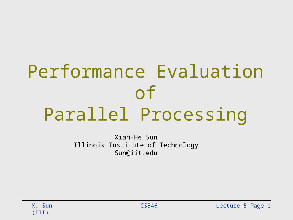
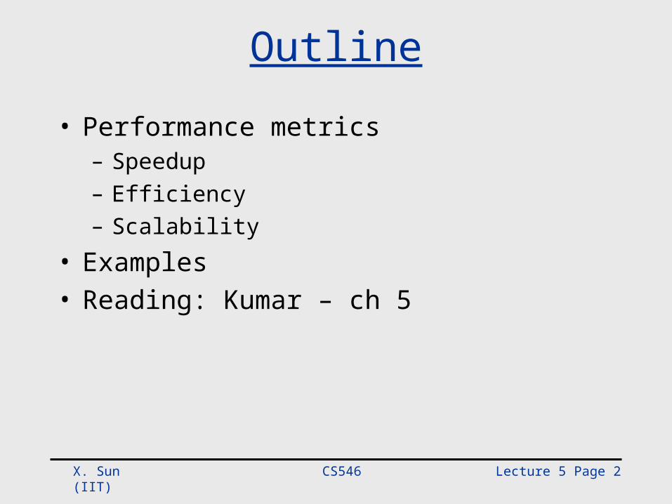
Outline

• Performance metrics– Speedup– Efficiency– Scalability

• Examples• Reading: Kumar – ch 5


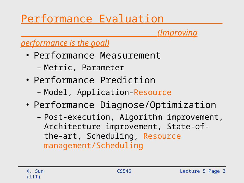
Performance Evaluation (Improving performance is the goal)

• Performance Measurement– Metric, Parameter

• Performance Prediction– Model, Application-Resource

• Performance Diagnose/Optimization– Post-execution, Algorithm improvement,

Architecture improvement, State-of-the-art, Scheduling, Resource management/Scheduling


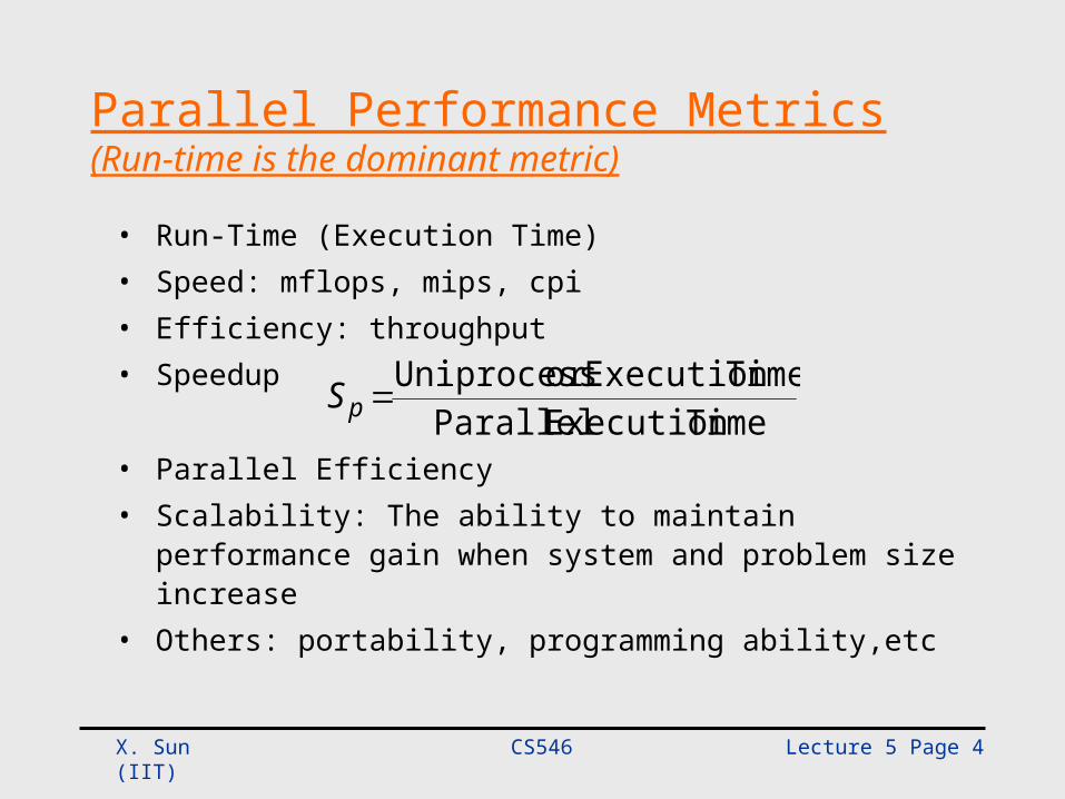
Parallel Performance Metrics(Run-time is the dominant metric)

• Run-Time (Execution Time)• Speed: mflops, mips, cpi• Efficiency: throughput • Speedup

• Parallel Efficiency• Scalability: The ability to maintain performance gain when

system and problem size increase• Others: portability, programming ability,etc

TimeExecutionParallelTimeExecutionorUniprocesspS


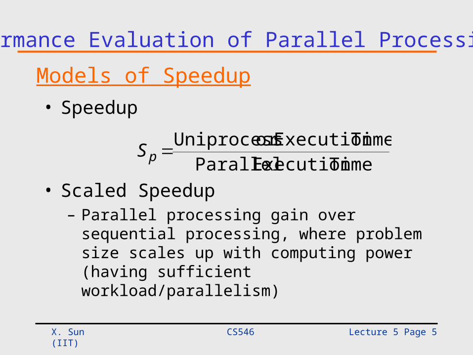
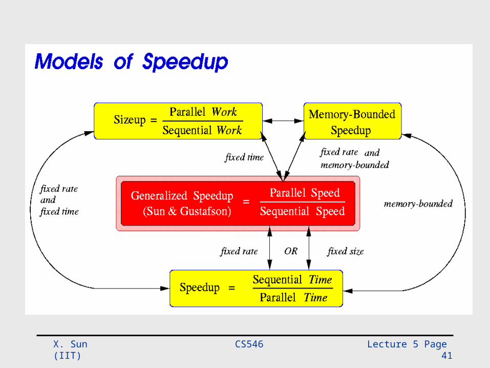
Models of Speedup• Speedup

• Scaled Speedup– Parallel processing gain over sequential

processing, where problem size scales up with computing power (having sufficient workload/parallelism)


Performance Evaluation of Parallel Processing


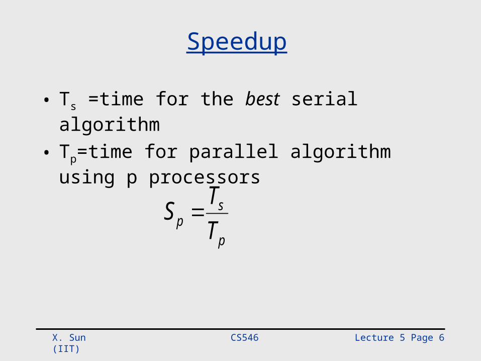
Speedup

• Ts =time for the best serial algorithm

• Tp=time for parallel algorithm using p processors

p

sp T

TS


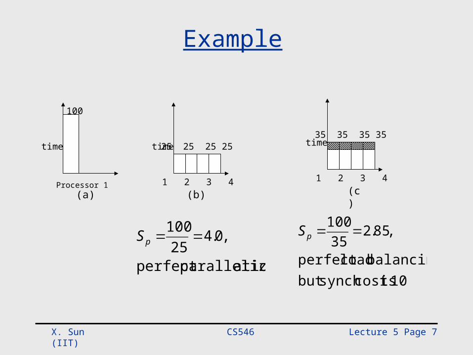
Example

Processor 1

time

100

time

1 2 3 4

25 25 25 25 time

1 2 3 4

35 35 35 35

(a) (b) (c)

ationparallelizperfect

,0.425

100pS

10 iscost synch but balancing loadperfect

,85.235

100pS


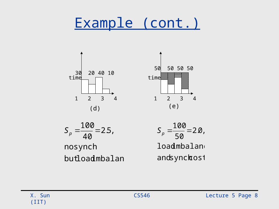
Example (cont.)

time

1 2 3 4

30 20 40 10 time

1 2 3 4

50 50 50 50

(d) (e)

imbalance loadbut synch no

,5.240

100pS

costsynch andimbalance load

,0.250

100pS


What Is “Good” Speedup?

• Linear speedup:

• Superlinear speedup

• Sub-linear speedup:

pS p

pS p

pS p


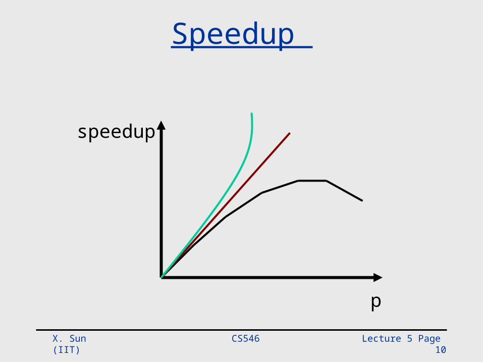
Speedup

p

speedup


Sources of Parallel Overheads • Interprocessor communication• Load imbalance• Synchronization• Extra computation


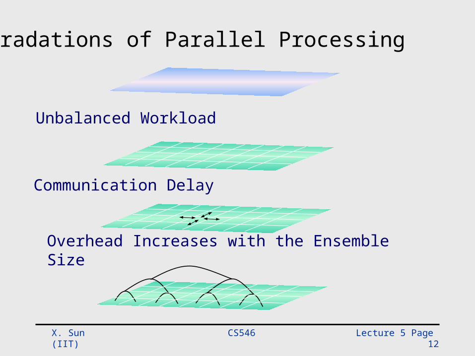
Degradations of Parallel Processing

Unbalanced Workload

Communication Delay

Overhead Increases with the Ensemble Size


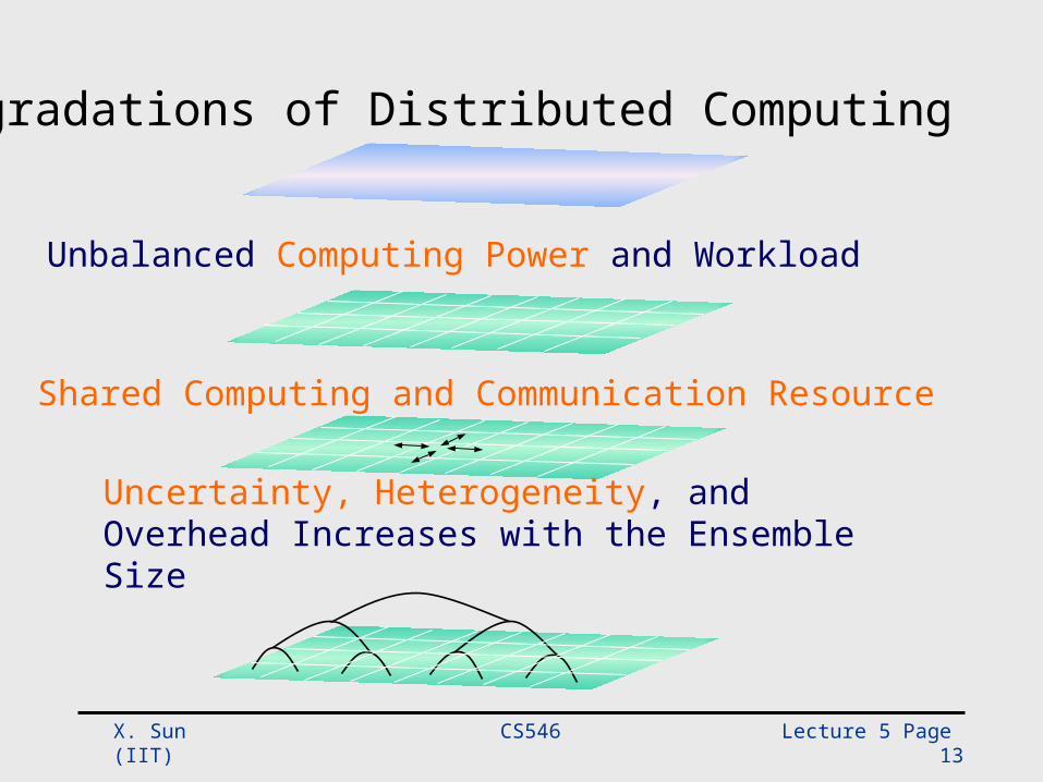
Degradations of Distributed Computing

Unbalanced Computing Power and Workload

Shared Computing and Communication Resource

Uncertainty, Heterogeneity, and Overhead Increases with the Ensemble Size


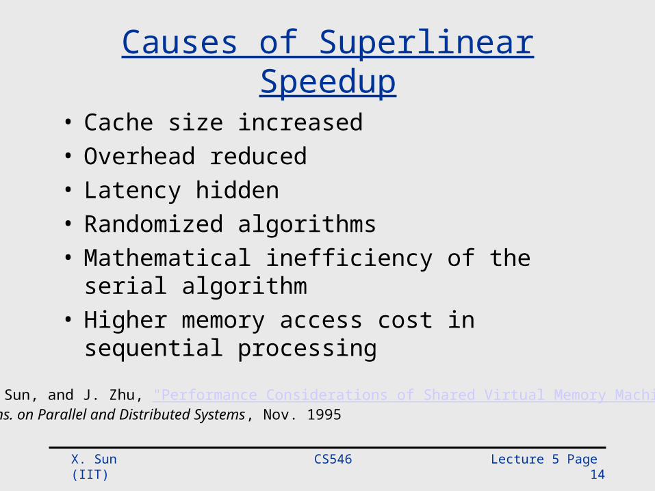
Causes of Superlinear Speedup

• Cache size increased• Overhead reduced• Latency hidden• Randomized algorithms• Mathematical inefficiency of the serial algorithm• Higher memory access cost in sequential

processing

• X.H. Sun, and J. Zhu, "Performance Considerations of Shared Virtual Memory Machines," IEEE Trans. on Parallel and Distributed Systems, Nov. 1995

http://www.cs.iit.edu/~scs/psfiles/ieee95.pdf


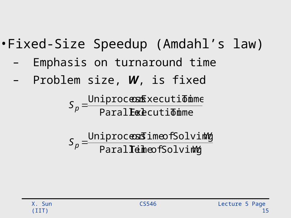
• Fixed-Size Speedup (Amdahl’s law)– Emphasis on turnaround time– Problem size, W, is fixed


WWS p SolvingofTimeParallel

SolvingofTimeorUniprocess


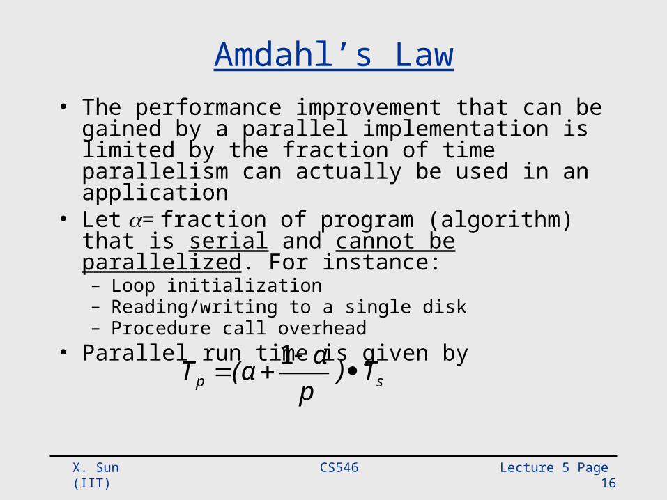
Amdahl’s Law• The performance improvement that can be gained by

a parallel implementation is limited by the fraction of time parallelism can actually be used in an application

• Let = fraction of program (algorithm) that is serial and cannot be parallelized. For instance:– Loop initialization– Reading/writing to a single disk– Procedure call overhead

• Parallel run time is given by

sp T)p

α(αT

1


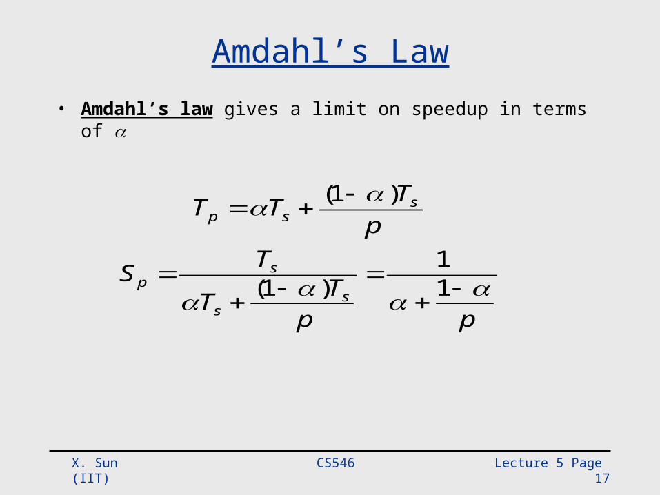
Amdahl’s Law• Amdahl’s law gives a limit on speedup in terms of

ppTT

TS

pTTT

ss

sp

ssp

11

)1(

)1(


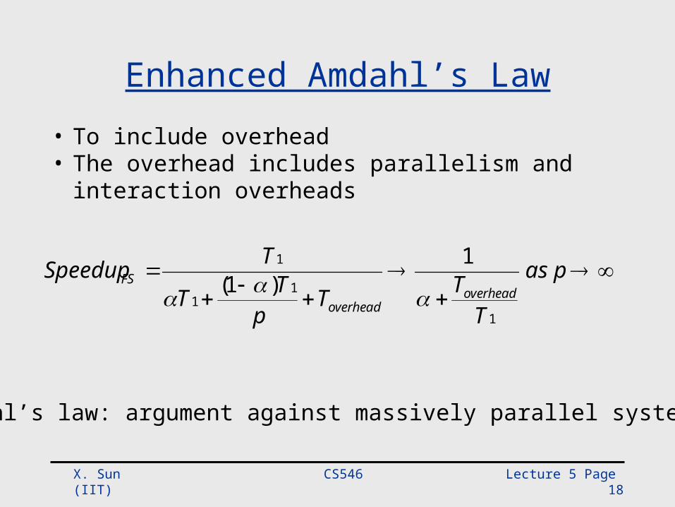
Enhanced Amdahl’s Law

pas

TTT

pTT

TSpeedupoverhead

overhead

FS

1

11

1 1)1(

• To include overhead• The overhead includes parallelism and interaction

overheads

Amdahl’s law: argument against massively parallel systems


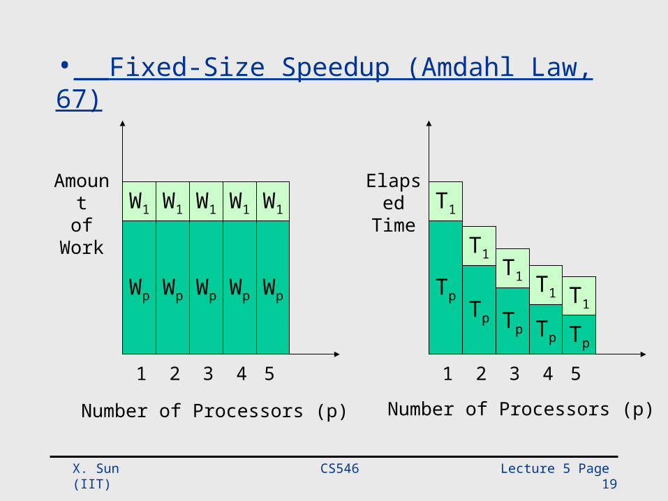
• Fixed-Size Speedup (Amdahl Law, 67)

Wp

W1

Wp Wp WpWp

W1 W1 W1 W1

1 2 3 4 5

Number of Processors (p)

Amount

ofWork

Tp

T1

Tp Tp Tp

T1T1

Tp

T1 T1

1 2 3 4 5

Number of Processors (p)

ElapsedTime


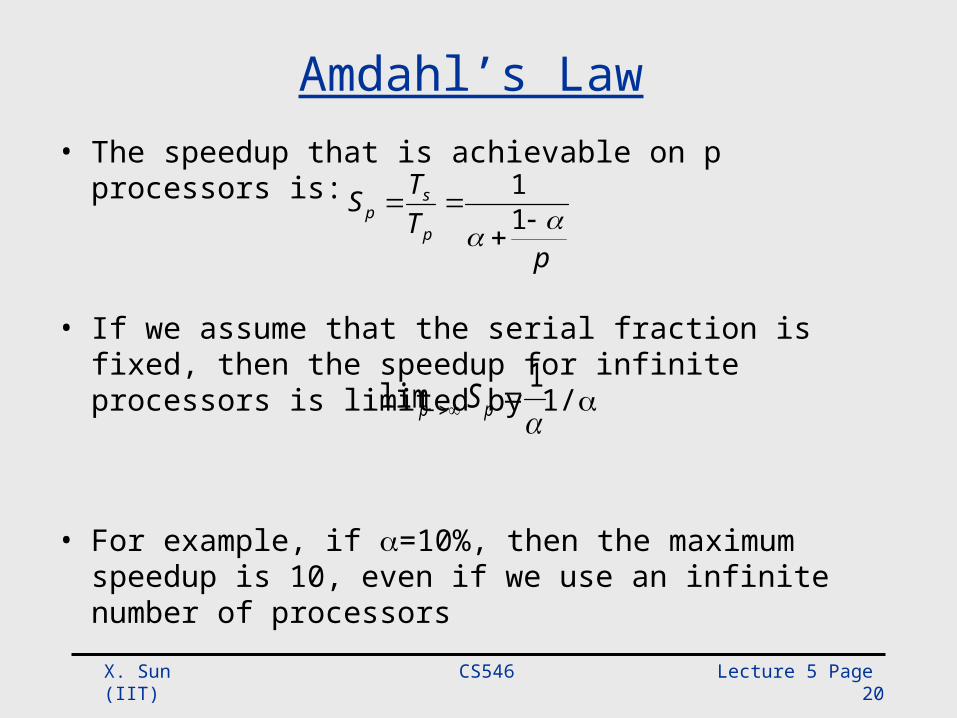
Amdahl’s Law• The speedup that is achievable on p processors is:

• If we assume that the serial fraction is fixed, then the speedup for infinite processors is limited by 1/

• For example, if =10%, then the maximum speedup is 10, even if we use an infinite number of processors

pTTS

p

sp

1

1

1lim pp S


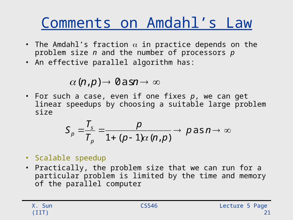
Comments on Amdahl’s Law• The Amdahl’s fraction in practice depends on the problem

size n and the number of processors p• An effective parallel algorithm has:

• For such a case, even if one fixes p, we can get linear speedups by choosing a suitable large problem size

• Scalable speedup• Practically, the problem size that we can run for a particular

problem is limited by the time and memory of the parallel computer

npn as 0),(

nppnp

pTTS

p

sp as

),()1(1


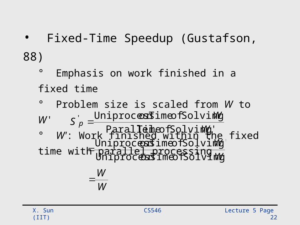
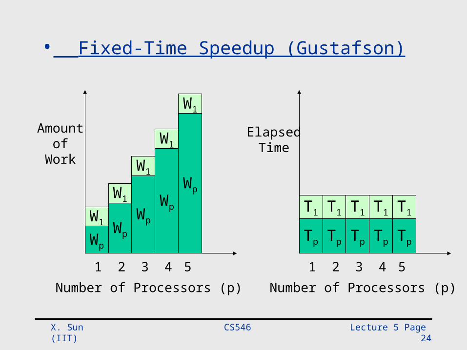
• Fixed-Time Speedup (Gustafson, 88)° Emphasis on work finished in a fixed time° Problem size is scaled from W to W'° W': Work finished within the fixed time with parallel processing

WW

SolvingofTimeorUniprocess'SolvingofTimeorUniprocess

'SolvingofTimeParallel'SolvingofTimeorUniprocess'

WWS p

WW '


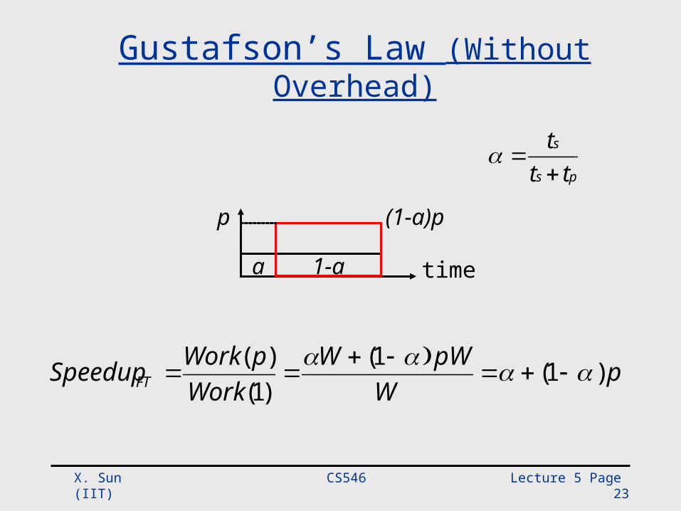
Gustafson’s Law (Without Overhead)

a 1-a time

p (1-a)p

ps

s

ttt

pW

pWWWork

pWorkSpeedupFT )1(1()1()(


• Fixed-Time Speedup (Gustafson)

Wp

W1 Wp

Wp

WpWp

W1

W1

W1

W1

1 2 3 4 5Number of Processors (p)

Amountof

Work

Tp

T1

Tp Tp Tp

T1 T1

Tp

T1 T1


ElapsedTime


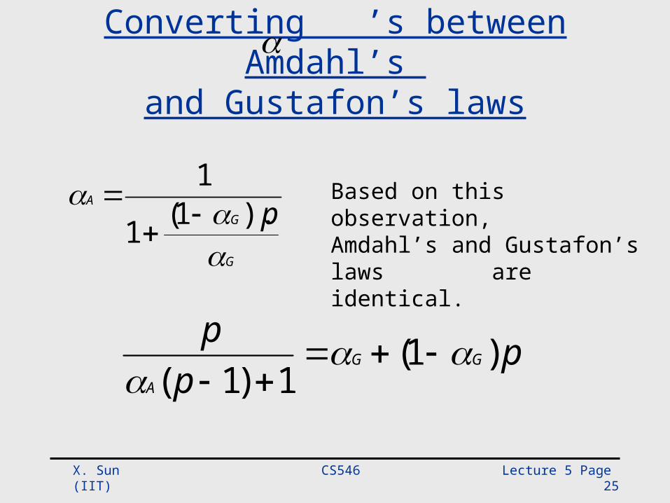
Converting ’s between Amdahl’s and Gustafon’s laws

Based on this observation, Amdahl’s and Gustafon’s laws are identical.

pp

pGG

A

)1(1)1(

G

GA p

).1(1

1


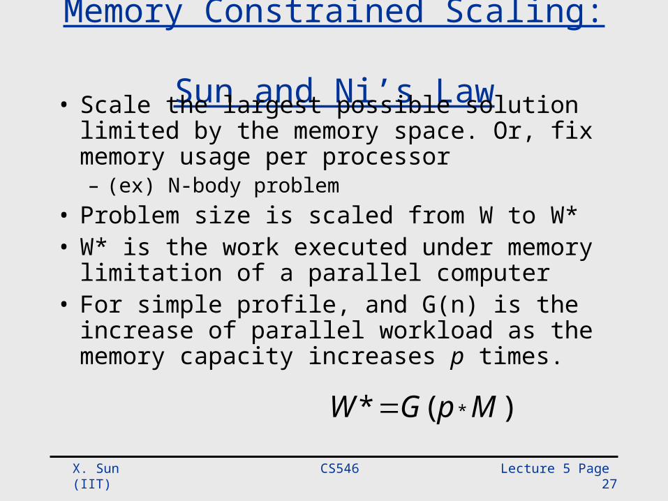
Memory Constrained Scaling: Sun and Ni’s Law

• Scale the largest possible solution limited by the memory space. Or, fix memory usage per processor– (ex) N-body problem

• Problem size is scaled from W to W*• W* is the work executed under memory

limitation of a parallel computer• For simple profile, and G(n) is the increase of

parallel workload as the memory capacity increases p times.

)(* * MpGW


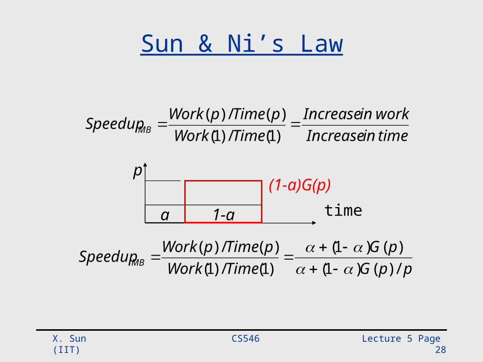
Sun & Ni’s Law

timeinIncreaseworkinIncrease

TimeWorkpTimepWorkSpeedupMB )1(/)1()(/)(

ppGpG

TimeWorkpTimepWorkSpeedupMB /)()1(

)()1()1(/)1()(/)(

a 1-a

p(1-a)G(p)

time


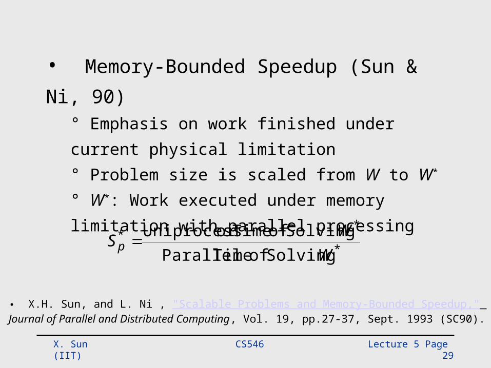
• Memory-Bounded Speedup (Sun & Ni, 90)° Emphasis on work finished under current physical limitation° Problem size is scaled from W to W*

° W*: Work executed under memory limitation with parallel processing

*

**

SolvingofTimeParallelSolvingofTimeorUniprocess

WWS p

• X.H. Sun, and L. Ni , "Scalable Problems and Memory-Bounded Speedup," Journal of Parallel and Distributed Computing, Vol. 19, pp.27-37, Sept. 1993 (SC90).

http://www.cs.iit.edu/~scs/psfiles/scalable93.pdf


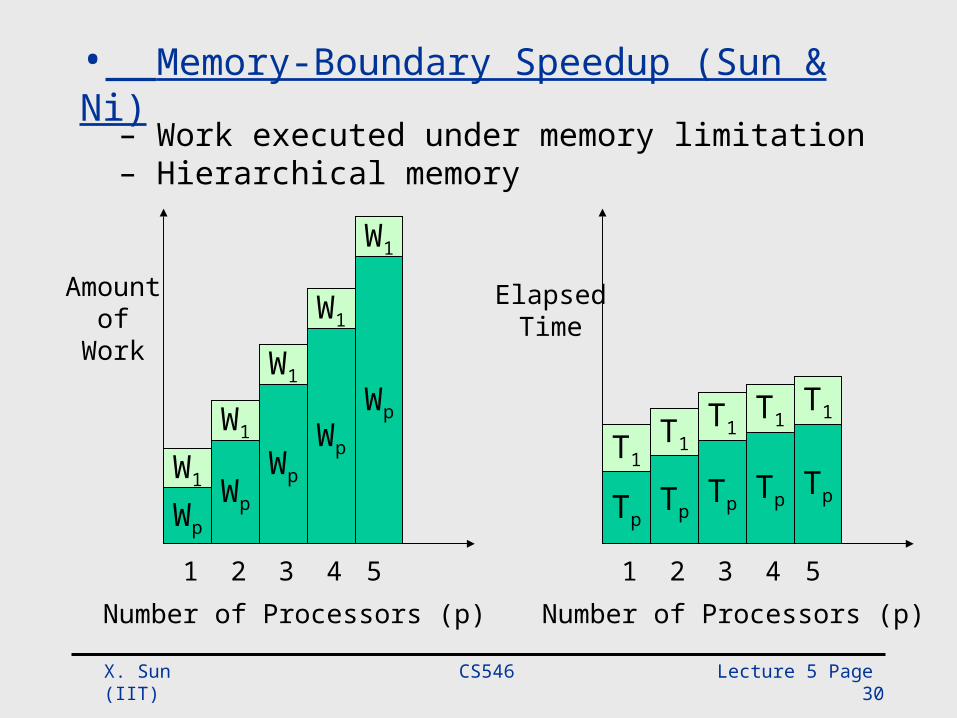
• Memory-Boundary Speedup (Sun & Ni)

Wp

W1 Wp

Wp

WpWp

W1

W1

W1

W1


Amountof

Work

Tp

T1

TpTp

Tp

T1T1

Tp

T1T1


ElapsedTime

– Work executed under memory limitation– Hierarchical memory


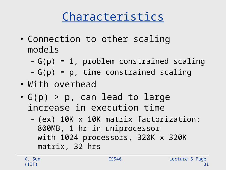
Characteristics

• Connection to other scaling models– G(p) = 1, problem constrained scaling– G(p) = p, time constrained scaling

• With overhead• G(p) > p, can lead to large increase in

execution time– (ex) 10K x 10K matrix factorization: 800MB, 1 hr in

uniprocessorwith 1024 processors, 320K x 320K matrix, 32 hrs


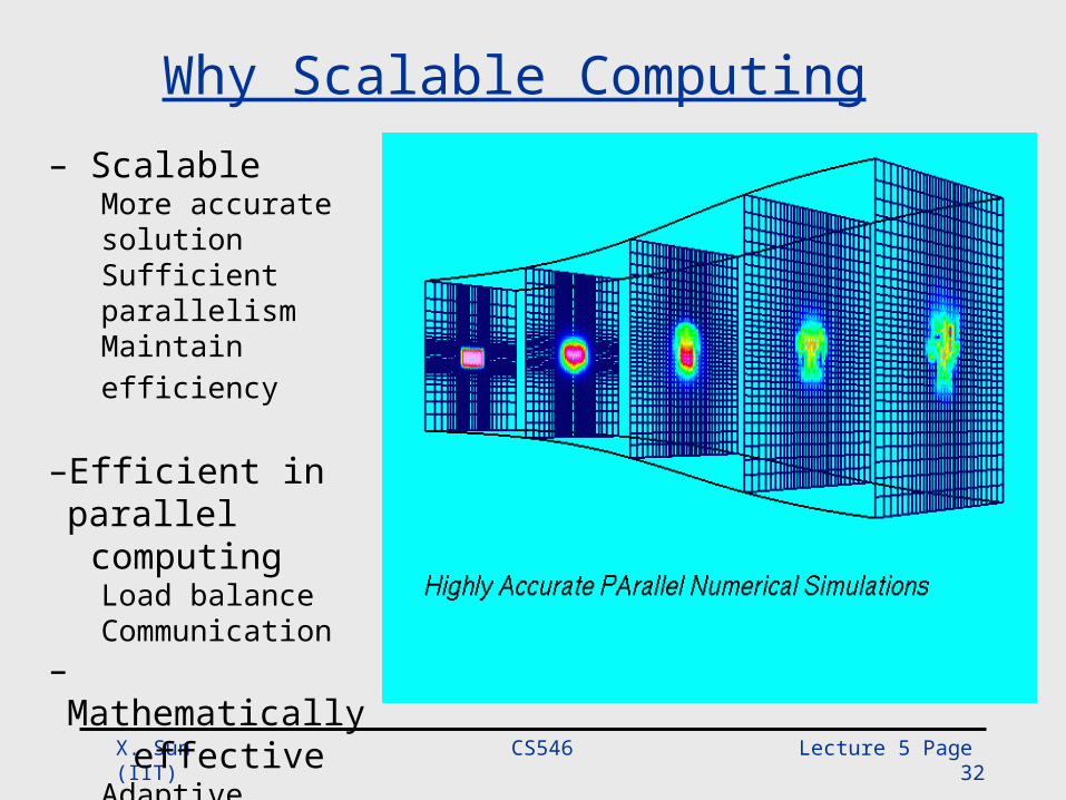
– ScalableMore accurate solutionSufficient parallelismMaintain efficiency

–Efficient in parallel computing

Load balanceCommunication

– Mathematically effective

AdaptiveAccuracy

Why Scalable Computing


• Memory-Bounded Speedup° Natural for domain decomposition based computing° Show the potential of parallel processing (In gerneal, computing requirement increases faster with problem size than that of communication)° Impacts extend to architecture design: trade-off of memory size and computing speed


Why Scalable Computing (2)

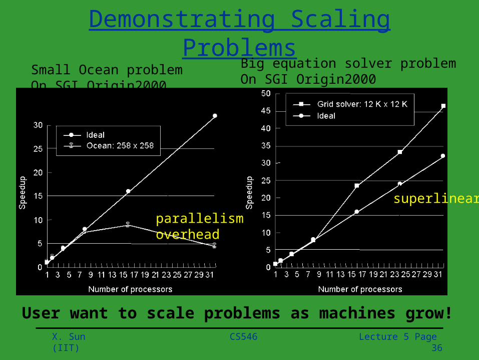
• Appropriate for small machine– Parallelism overheads begin to dominate benefits

for larger machines• Load imbalance• Communication to computation ratio

– May even achieve slowdowns– Does not reflect real usage, and inappropriate for

large machine• Can exaggerate benefits of improvements

Small Work


Why Scalable Computing (3)

• Appropriate for big machine– Difficult to measure improvement– May not fit for small machine

• Can’t run• Thrashing to disk• Working set doesn’t fit in cache

– Fits at some p, leading to superlinear speedup

Large Work


Demonstrating Scaling Problems

parallelism overhead

superlinear

User want to scale problems as machines grow!

Small Ocean problemOn SGI Origin2000

Big equation solver problemOn SGI Origin2000


How to Scale• Scaling a machine

– Make a machine more powerful– Machine size

• <processor, memory, communication, I/O>– Scaling a machine in parallel processing

• Add more identical nodes

• Problem size– Input configuration– data set size : the amount of storage required to

run it on a single processor– memory usage : the amount of memory used by

the program


Two Key Issues in Problem Scaling

• Under what constraints should the problem be scaled?– Some properties must be fixed as the machine

scales• How should the problem be scaled?

– Which parameters?– How?


Constraints To Scale

• Two types of constraints– Problem-oriented

• Ex) Time– Resource-oriented

• Ex) Memory

• Work to scale– Metric-oriented

• Floating point operation, instructions– User-oriented

• Easy to change but may difficult to compare• Ex) particles, rows, transactions• Difficult cross comparison


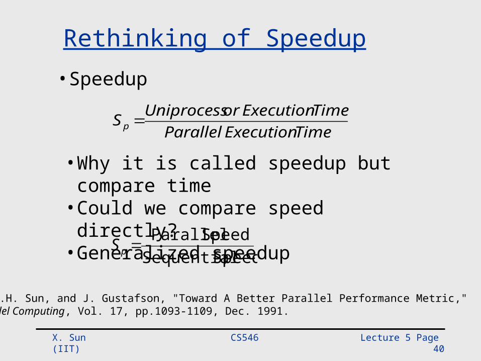
• Speedup

TimeExecutionParallelTimeExecutionorUniprocessS p

Speed SequentialSpeedParallel

pS

Rethinking of Speedup

• Why it is called speedup but compare time• Could we compare speed directly?• Generalized speedup

• X.H. Sun, and J. Gustafson, "Toward A Better Parallel Performance Metric," Parallel Computing, Vol. 17, pp.1093-1109, Dec. 1991.



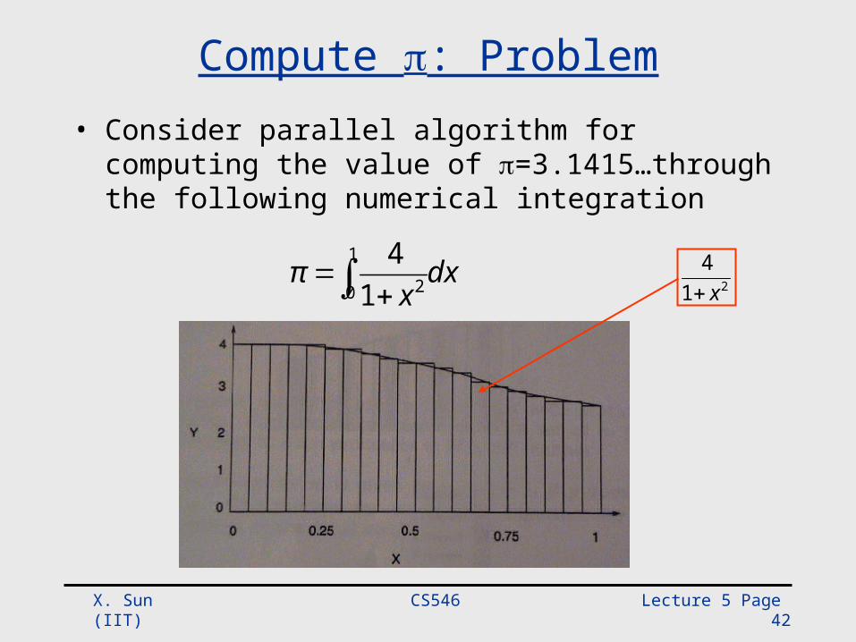
Compute : Problem• Consider parallel algorithm for computing the value of

=3.1415…through the following numerical integration

dxx

π

1

0 214

214x


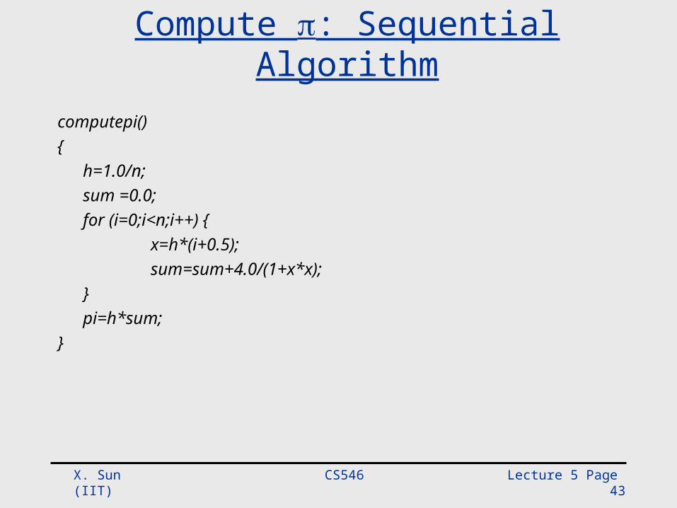
Compute : Sequential Algorithm

computepi(){

h=1.0/n;sum =0.0;for (i=0;i<n;i++) {

x=h*(i+0.5);sum=sum+4.0/(1+x*x);

}pi=h*sum;

}


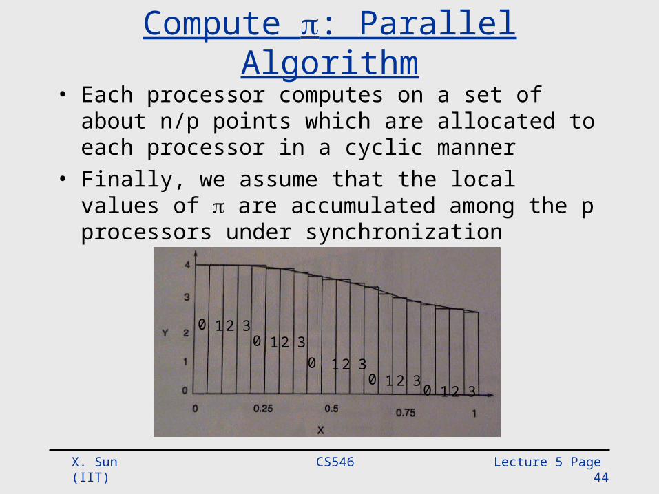
Compute : Parallel Algorithm• Each processor computes on a set of about n/p

points which are allocated to each processor in a cyclic manner

• Finally, we assume that the local values of are accumulated among the p processors under synchronization

0

1 2 3 0

1 2 3

0

1 2 3 0

1 2 3 0

1 2 3


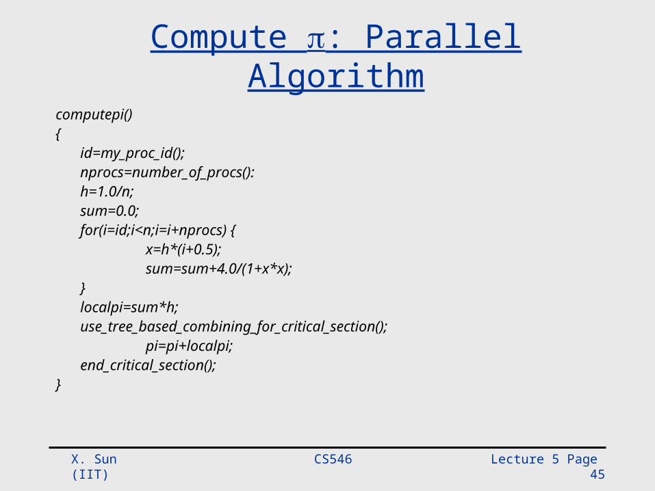
Compute : Parallel Algorithmcomputepi(){

id=my_proc_id();nprocs=number_of_procs():h=1.0/n;sum=0.0;for(i=id;i<n;i=i+nprocs) {

x=h*(i+0.5);sum=sum+4.0/(1+x*x);

}localpi=sum*h;use_tree_based_combining_for_critical_section();

pi=pi+localpi;end_critical_section();

}


Compute : Analysis

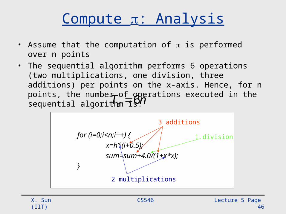
• Assume that the computation of is performed over n points• The sequential algorithm performs 6 operations (two

multiplications, one division, three additions) per points on the x-axis. Hence, for n points, the number of operations executed in the sequential algorithm is:

nTs 6

for (i=0;i<n;i++) {x=h*(i+0.5);sum=sum+4.0/(1+x*x);

}

3 additions

2 multiplications

1 division


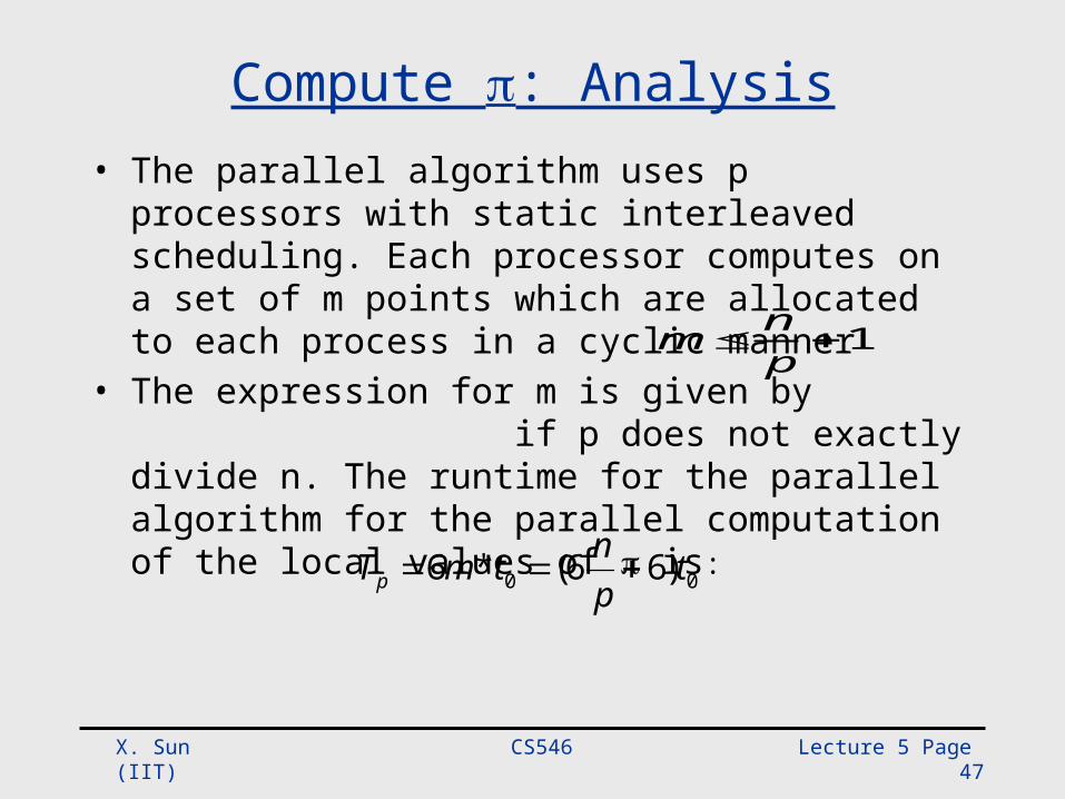
Compute : Analysis• The parallel algorithm uses p processors with static

interleaved scheduling. Each processor computes on a set of m points which are allocated to each process in a cyclic manner

• The expression for m is given by if p does not exactly divide n. The runtime for the parallel algorithm for the parallel computation of the local values of is:

1pnm

00 )66(*6 tpntmTp


Compute : Analysis

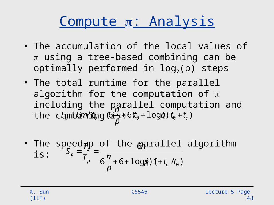
• The accumulation of the local values of using a tree-based combining can be optimally performed in log2(p) steps

• The total runtime for the parallel algorithm for the computation of including the parallel computation and the combining is:

• The speedup of the parallel algorithm is:

))(log()66(*6 000 cp ttptpntmT

)/1)(log(66

6

0ttppn

nTTS

cp

sp


Compute : Analysis

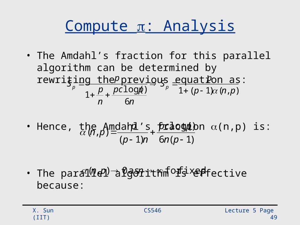
• The Amdahl’s fraction for this parallel algorithm can be determined by rewriting the previous equation as:

• Hence, the Amdahl’s fraction (n,p) is:

• The parallel algorithm is effective because:

),()1(16

)log(1 pnppS

nppc

np

pS pp

)1(6)log(

)1(),(

pnppc

npppn

pnpn fixedfor as 0),(


Finite Differences: Problem

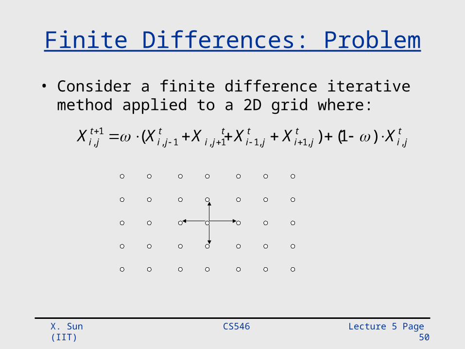
• Consider a finite difference iterative method applied to a 2D grid where:

tji

tji

tji

tji

tji

tji XXXXXX ,,1,11,1,1

, )1()(


Finite Differences: Serial Algorithm

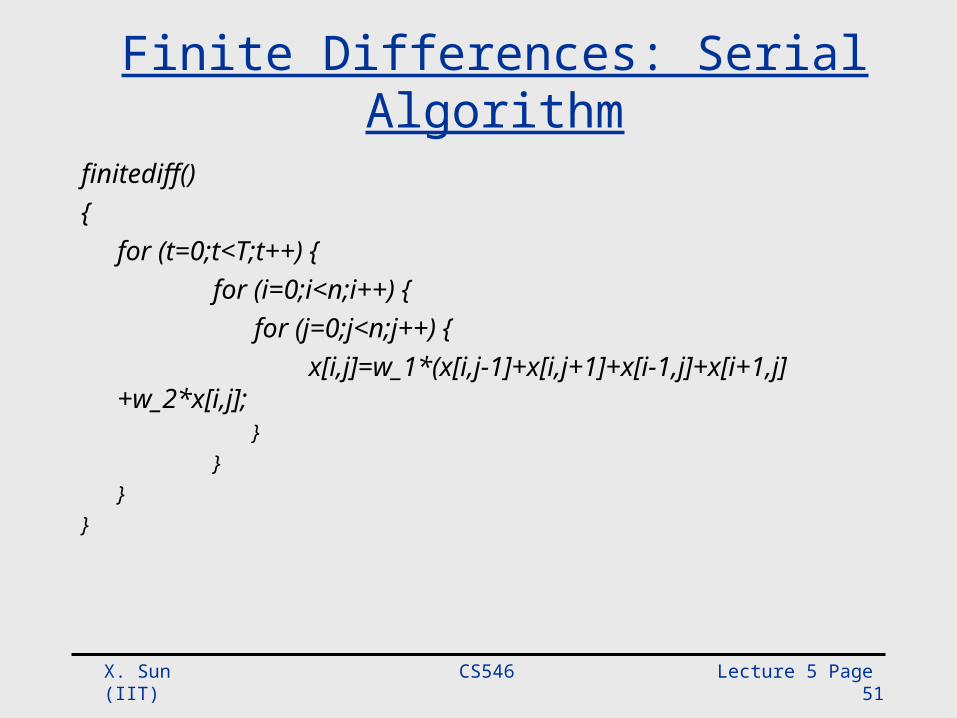
finitediff(){

for (t=0;t<T;t++) {for (i=0;i<n;i++) { for (j=0;j<n;j++) {

x[i,j]=w_1*(x[i,j-1]+x[i,j+1]+x[i-1,j]+x[i+1,j]+w_2*x[i,j];

}}

}}


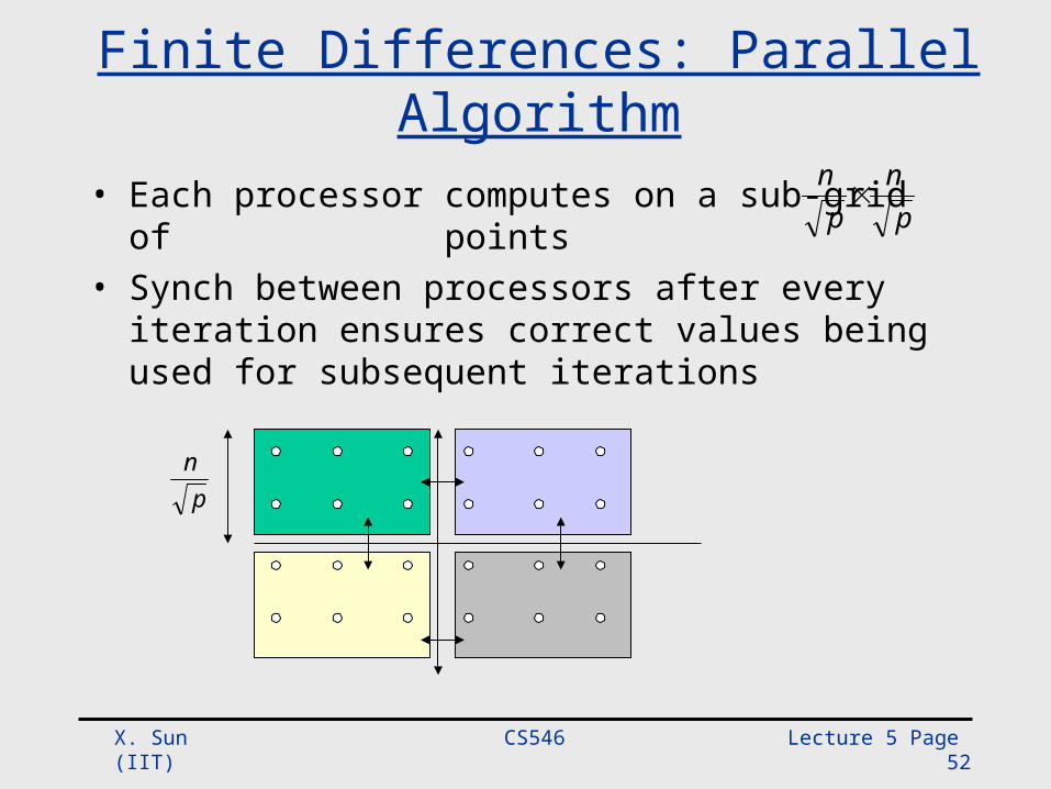
Finite Differences: Parallel Algorithm

• Each processor computes on a sub-grid of points

• Synch between processors after every iteration ensures correct values being used for subsequent iterations

pn

pn

pn


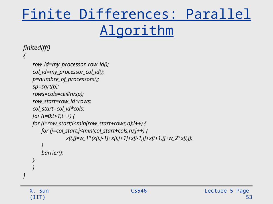
Finite Differences: Parallel Algorithm

finitediff(){

row_id=my_processor_row_id();col_id=my_processor_col_id();p=numbre_of_processors();sp=sqrt(p);rows=cols=ceil(n/sp);row_start=row_id*rows;col_start=col_id*cols;for (t=0;t<T;t++) {for (i=row_start;i<min(row_start+rows,n);i++) { for (j=col_start;j<min(col_start+cols,n);j++) { x[i,j]=w_1*(x[i,j-1]+x[i,j+1]+x[i-1,j]+x[i+1,j]+w_2*x[i,j]; } barrier();}}

}


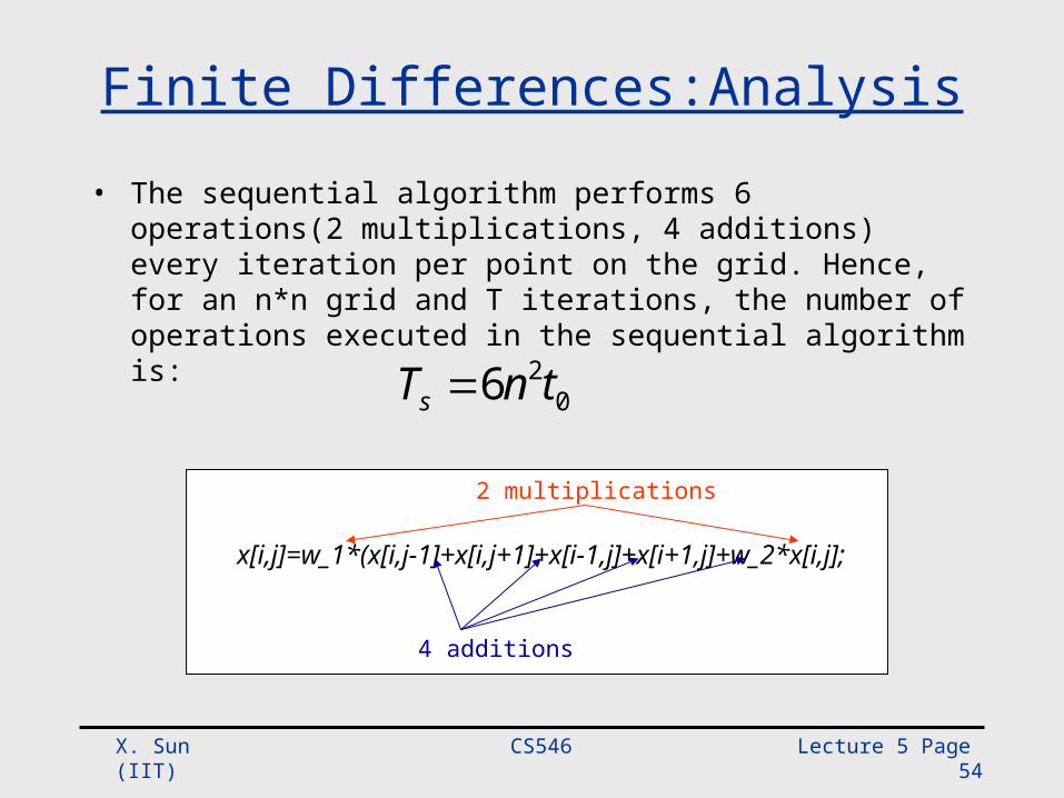
Finite Differences:Analysis

• The sequential algorithm performs 6 operations(2 multiplications, 4 additions) every iteration per point on the grid. Hence, for an n*n grid and T iterations, the number of operations executed in the sequential algorithm is:

026 tnTs

x[i,j]=w_1*(x[i,j-1]+x[i,j+1]+x[i-1,j]+x[i+1,j]+w_2*x[i,j];

2 multiplications

4 additions


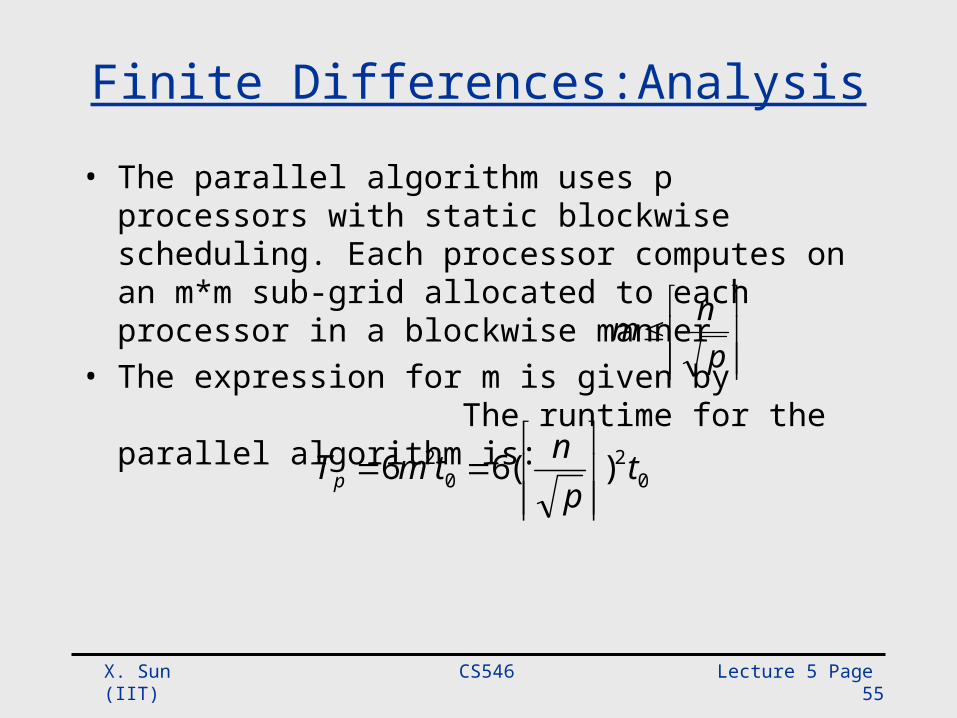
Finite Differences:Analysis

• The parallel algorithm uses p processors with static blockwise scheduling. Each processor computes on an m*m sub-grid allocated to each processor in a blockwise manner

• The expression for m is given by The runtime for the parallel algorithm is:

pnm

02

02 )(66 t

pntmTp


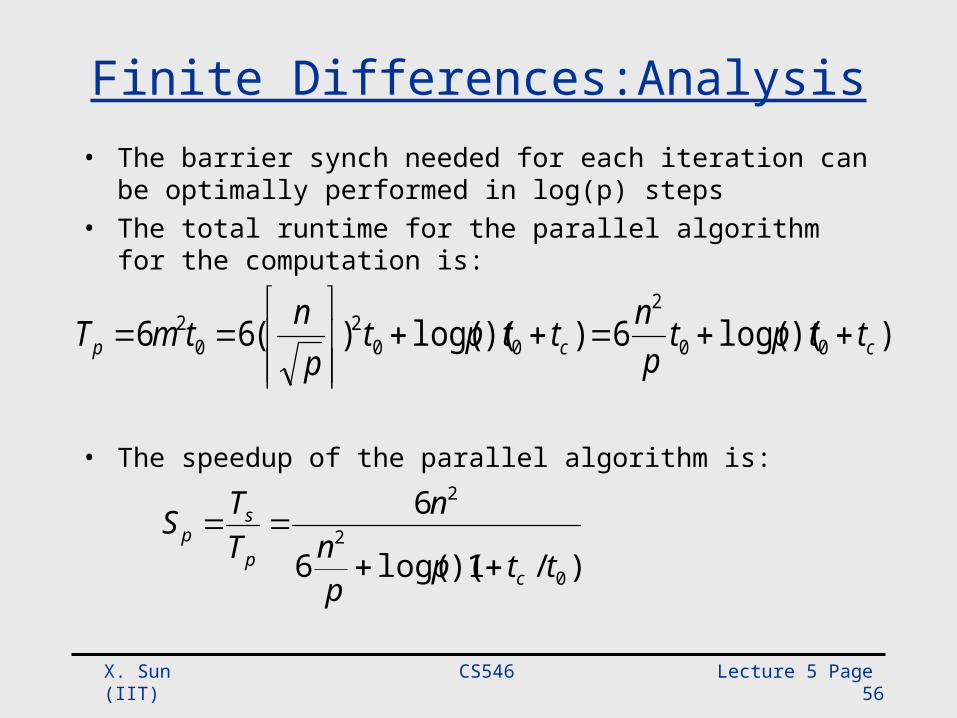
Finite Differences:Analysis• The barrier synch needed for each iteration can be optimally

performed in log(p) steps• The total runtime for the parallel algorithm for the computation

is:

• The speedup of the parallel algorithm is:

))(log(6))(log()(66 00

2

002

02

ccp ttptp

nttptp

ntmT

)/1)(log(6

6

0

2

2

ttpp

nn

TTS

cp

sp


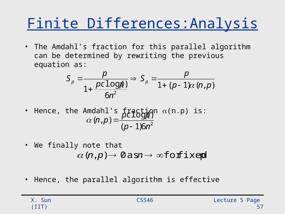
Finite Differences:Analysis• The Amdahl’s fraction for this parallel algorithm can be

determined by rewriting the previous equation as:

• Hence, the Amdahl’s fraction (n.p) is:

• We finally note that

• Hence, the parallel algorithm is effective

),()1(16

)log(1 2pnp

pS

nppc

pS pp

26)1()log(),(

npppcpn

p fixedfor as 0),( npn


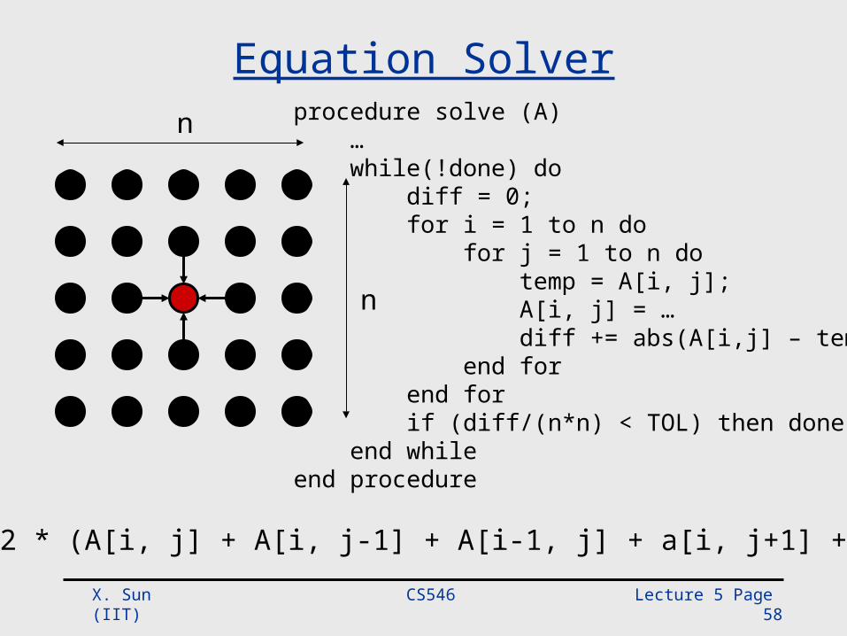
Equation Solver

A[i,j] = 0.2 * (A[i, j] + A[i, j-1] + A[i-1, j] + a[i, j+1] + a[i+1, j])

n

n procedure solve (A) … while(!done) do diff = 0; for i = 1 to n do for j = 1 to n do temp = A[i, j]; A[i, j] = … diff += abs(A[i,j] – temp); end for end for if (diff/(n*n) < TOL) then done =1 ; end whileend procedure


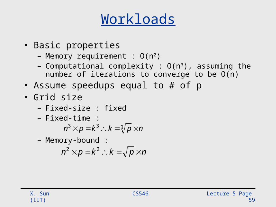
Workloads

• Basic properties– Memory requirement : O(n2)– Computational complexity : O(n3), assuming the number of

iterations to converge to be O(n)• Assume speedups equal to # of p• Grid size

– Fixed-size : fixed– Fixed-time :

– Memory-bound : npkkpn 333

npkkpn 22


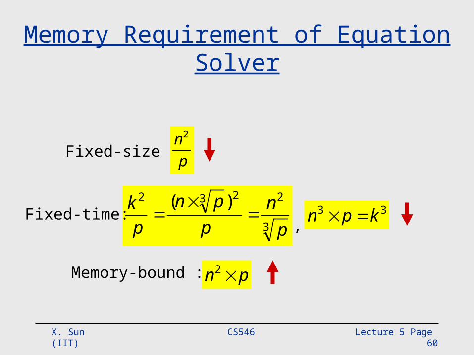
Memory Requirement of Equation Solver

3

2232 )(

pn

ppn

pk

Fixed-time: 33 kpn

Fixed-size :

Memory-bound : pn 2

,

pn2


Time Complexity of Equation Solver

Fixed-time:

Fixed-size:

Memory-bound:

22 kpn 33 )( pnk

Sequential time complexity

,

pn3

3n

pnppn 3

3)(


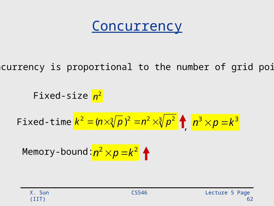
Concurrency

Fixed-time:

Fixed-size :

Memory-bound: 22 kpn

2n

Concurrency is proportional to the number of grid points

33 kpn 3 22232 )( pnpnk ,


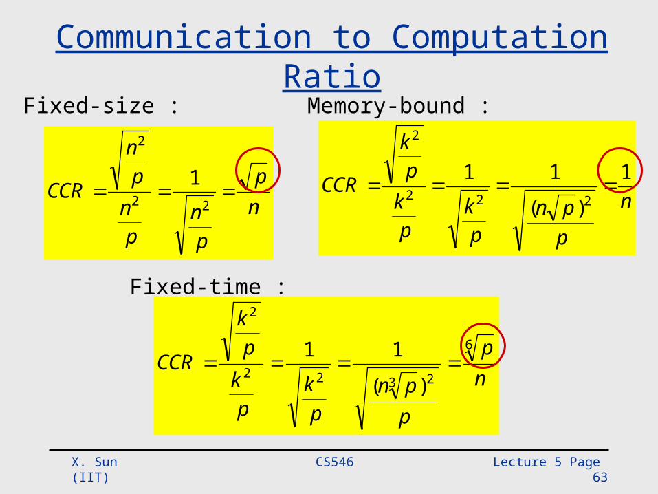
Communication to Computation Ratio

np

pn

pn

pn

CCR 22

2

1

Fixed-time :

Fixed-size : Memory-bound :

np

ppn

pk

pk

pk

CCR6

2322

2

)(

11

n

ppn

pk

pk

pk

CCR 1

)(

11222

2


Scalability

• The Need for New Metrics

• Comparison of performances with different workload

• Availability of massively parallel processing

• ScalabilityAbility to maintain parallel processing gain when both

problem size and system size increase


Parallel Efficiency

• The achieved fraction of total potential parallel processing gain– Assuming linear speedup p is ideal case

• The ability to maintain efficiency when problem size increase

pS

E pp


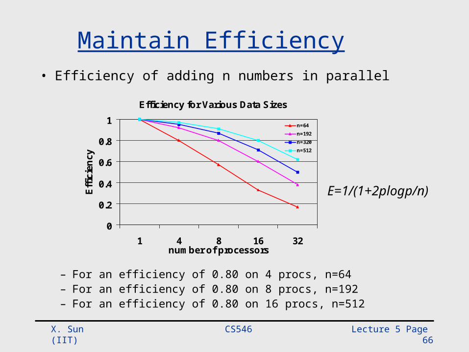
Maintain Efficiency• Efficiency of adding n numbers in parallel

– For an efficiency of 0.80 on 4 procs, n=64– For an efficiency of 0.80 on 8 procs, n=192– For an efficiency of 0.80 on 16 procs, n=512

Efficiency for Various Data Sizes

0

0.2

0.4

0.6

0.8

1

1 4 8 16 32number of processors

Effic

ienc

y

n=64n=192n=320n=512

E=1/(1+2plogp/n)


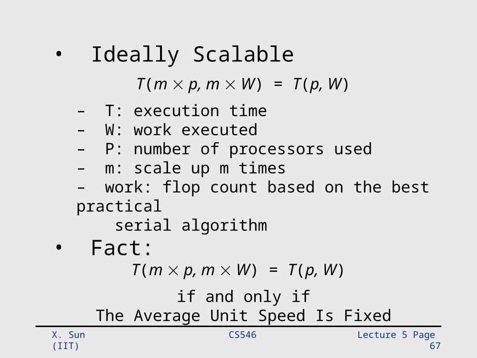
• Ideally ScalableT(m p, m W) = T(p, W)

– T: execution time– W: work executed– P: number of processors used– m: scale up m times– work: flop count based on the best practical serial algorithm

• Fact:T(m p, m W) = T(p, W)

if and only ifThe Average Unit Speed Is Fixed


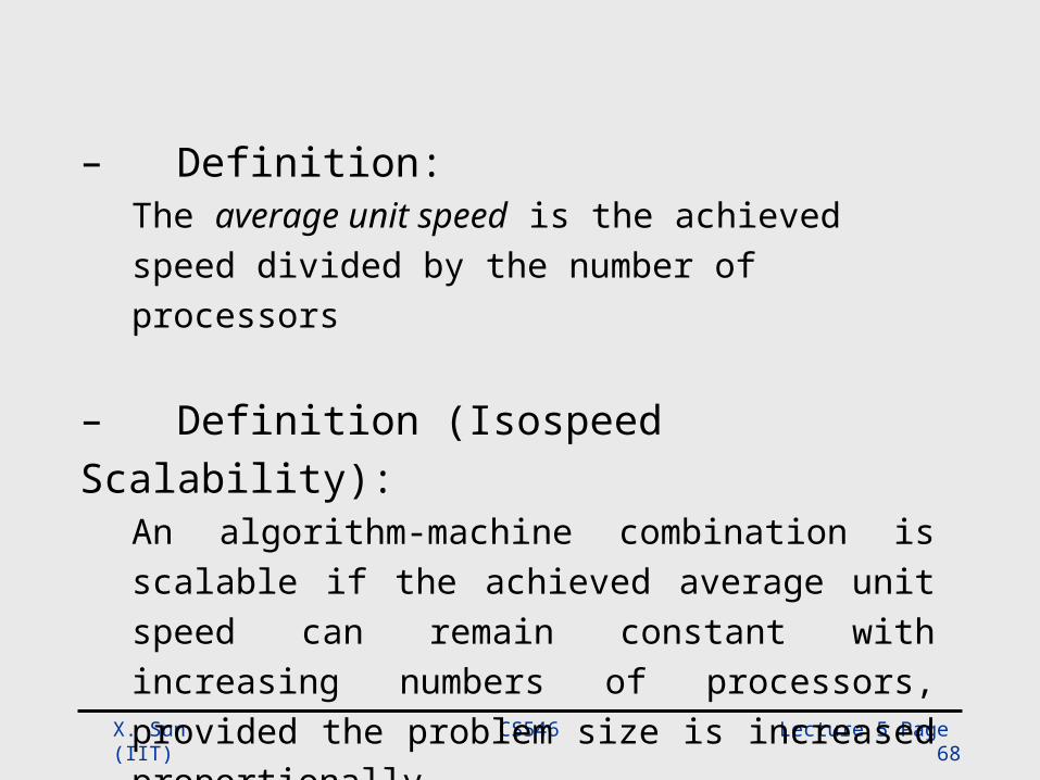
– Definition:The average unit speed is the achieved speed divided by the number of processors

– Definition (Isospeed Scalability):An algorithm-machine combination is scalable if the achieved average unit speed can remain constant with increasing numbers of processors, provided the problem size is increased proportionally


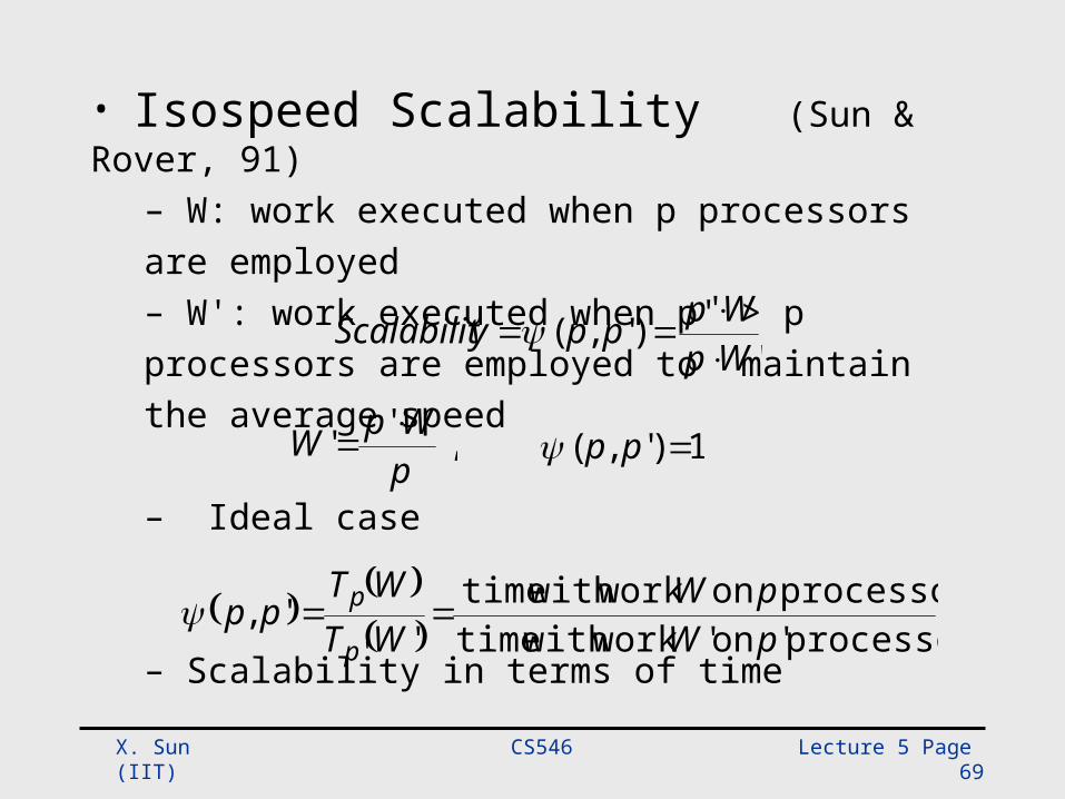
• Isospeed Scalability (Sun & Rover, 91)– W: work executed when p processors are employed– W': work executed when p' > p processors are employed to maintain the average speed

– Ideal case

– Scalability in terms of time

'')',(WpWpppyScalabilit

,''pWpW

processors'on'workwithtime

processorsonworkwithtime'

',' pW

pWWTWT

ppp

p

1)',( pp


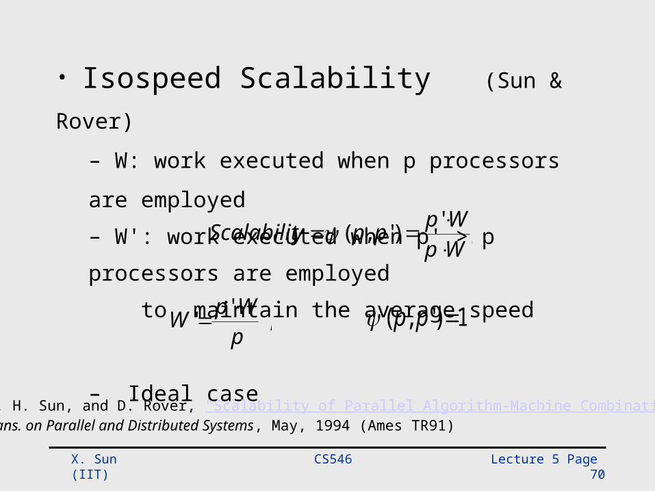
• Isospeed Scalability (Sun & Rover)

– W: work executed when p processors are employed

– W': work executed when p' > p processors are employed

to maintain the average speed

– Ideal case

'')',(WpWpppyScalabilit

,''pWpW 1)',( pp

• X. H. Sun, and D. Rover, "Scalability of Parallel Algorithm-Machine Combinations," IEEE Trans. on Parallel and Distributed Systems, May, 1994 (Ames TR91)

http://www.cs.iit.edu/~scs/psfiles/scalability94.pdf


The Relation of Scalability and Time

• More scalable leads to smaller time– Better initial run-time and higher scalability lead to

superior run-time– Same initial run-time and same scalability lead to

same scaled performance– Superior initial performance may not last long if

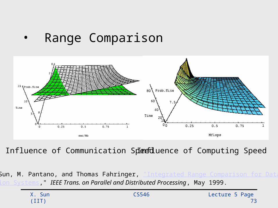
scalability is low• Range Comparison

• X.H. Sun, "Scalability Versus Execution Time in Scalable Systems," Journal of Parallel and Distributed Computing, Vol. 62, No. 2, pp. 173-192, Feb 2002.

http://www.cs.iit.edu/~scs/psfiles/scalability2002.pdf


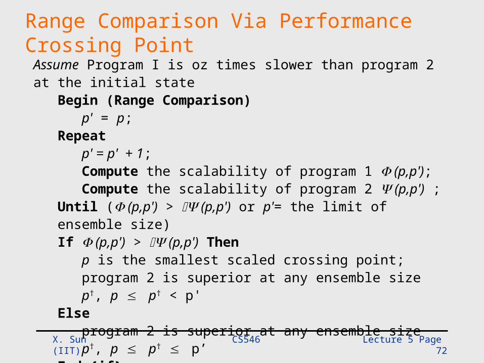
Range Comparison Via Performance Crossing PointAssume Program I is oz times slower than program 2 at the initial state

Begin (Range Comparison)p' = p;

Repeatp' = p' + 1;Compute the scalability of program 1 (p,p');Compute the scalability of program 2 (p,p') ;

Until ( (p,p') > (p,p') or p'= the limit of ensemble size)If (p,p') > (p,p') Then

p is the smallest scaled crossing point;program 2 is superior at any ensemble size p†, p p† < p'

Elseprogram 2 is superior at any ensemble size p†, p p† p’

End {if}End {Range Comparison}


• Range Comparison

Influence of Communication Speed Influence of Computing Speed

• X.H. Sun, M. Pantano, and Thomas Fahringer, "Integrated Range Comparison for Data-Parallel Compilation Systems," IEEE Trans. on Parallel and Distributed Processing, May 1999.

http://www.cs.iit.edu/~scs/SCALA/range.pdf

http://www.cs.iit.edu/~scs/SCALA/range.pdf


The SCALA (SCALability Analyzer) System

• Design Goals– Predict performance– Support program optimization– Estimate the influence of hardware variations

• Uniqueness– Designed to be integrated into advanced compiler

systems– Based on scalability analysis


• Vienna Fortran Compilation System– A data-parallel restructuring compilation system– Consists of a parallelizing compiler for VF/HPF

and tools for program analysis and restructuring– Under a major upgrade for HPF2

• Performance prediction is crucial for appropriate program restructuring


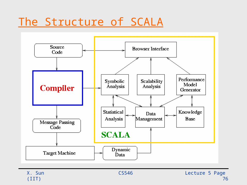
The Structure of SCALA


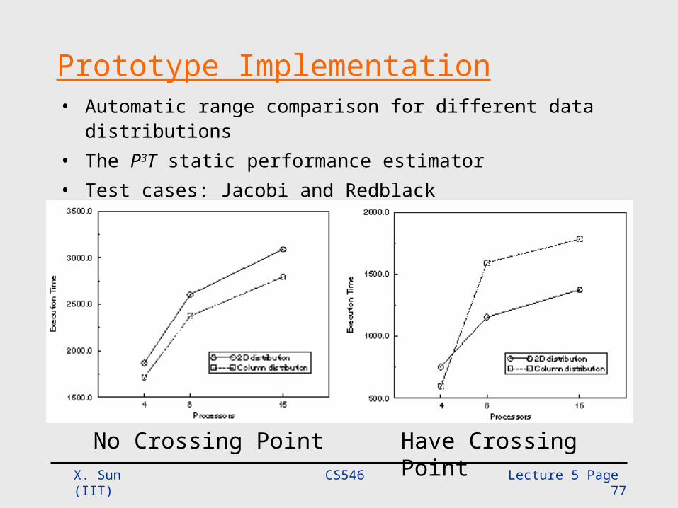
Prototype Implementation• Automatic range comparison for different data distributions• The P3T static performance estimator• Test cases: Jacobi and Redblack

No Crossing Point Have Crossing Point


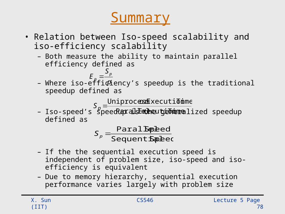
Summary• Relation between Iso-speed scalability and iso-

efficiency scalability– Both measure the ability to maintain parallel efficiency

defined as – Where iso-efficiency’s speedup is the traditional speedup

defined as

– Iso-speed’s speedup is the generalized speedup defined as

– If the the sequential execution speed is independent of problem size, iso-speed and iso-efficiency is equivalent

– Due to memory hierarchy, sequential execution performance varies largely with problem size

pS

E pp

Speed SequentialSpeed Parallel

pS



Summary

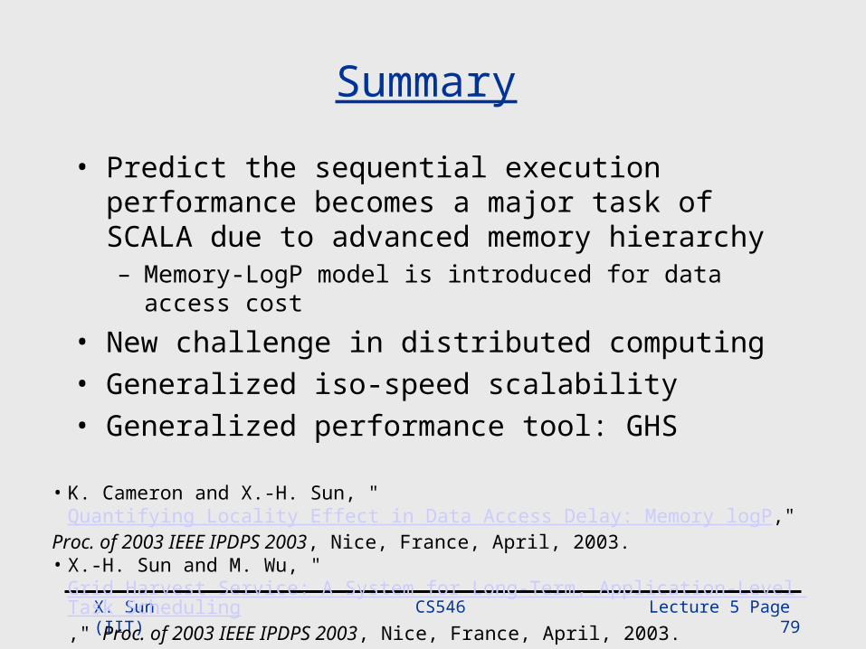
• Predict the sequential execution performance becomes a major task of SCALA due to advanced memory hierarchy – Memory-LogP model is introduced for data access cost

• New challenge in distributed computing• Generalized iso-speed scalability• Generalized performance tool: GHS

• K. Cameron and X.-H. Sun, "Quantifying Locality Effect in Data Access Delay: Memory logP," Proc. of 2003 IEEE IPDPS 2003, Nice, France, April, 2003. • X.-H. Sun and M. Wu, "

Grid Harvest Service: A System for Long-Term, Application-Level Task Scheduling," Proc. of 2003 IEEE IPDPS 2003, Nice, France, April, 2003.

http://www.cs.iit.edu/~scs/psfiles/KSipdps03.PDF

http://www.cs.iit.edu/~scs/psfiles/KSipdps03.PDF

http://www.cs.iit.edu/~scs/psfiles/SWipdps03.PDF

Documents

Dynamic Load Balancing for Parallel and Distributed Systems