Dynamic modeling and control of the main metabolism in Lactic acidbacteria

Bhabuk Koirala1,2,∗, Isabel Sá-Correia1, Rafael Costa2, Susana Vinga2

1 Instituto Superior Téchnico, Lisbon, Portugal2 INESC - ID, Lisbon, Portugal

∗ E-mail: koirala.bhabuk@gmail.com

Abstract

Lactic acid bacteria (LAB) are widely used in industrial manufacture of fermented foods and regardedas cell factories for production of pharmaceutical and food products. Lactococcus lactis, due to its smallgenome size and simple metabolism, has been considered a model organism for strain design strategiesand metabolic engineering. Metabolic modeling provides a platform to conduct in silico experiments withbiotechnological and biomedical applications. With a fully detailed kinetic model, time-course simulations,response to different input can be predicted and system controllers can be designed. For L. lactis, thedynamic models for the central carbon metabolism have already been constructed. However, these modelslack our compound of interest and need to be extended. Provided the topology of pathway and kineticparameters, a dynamic model that describes the glycolytic pathway in L. lactis is reconstructed usingconvenience kinetics. This model is now improved by estimating the parameters using in vivo NuclearMagnetic Resonance (NMR) data fitting. Sensitivity analysis was performed in the reconstructed modelfor acetoin and butanediol production which suggests that down expression of the enzyme levels for lactatedehydrogenase, phosphofructokinase, pyruvate dehydrogenase causes a rise in production of acetoin and2,3-butanediol. In addition to these enzyme levels, down expression of acetoin transportase and alcoholdehydrogenase levels accounts for enhanced production of 2,3-butanediol.

The reconstructed model can be used as a basis to design metabolic engineering experiments and alsoto predict the phenotype of the bacterium under different environmental and genetic conditions. Themodel can also serve as a starting point to model other LAB for instance Streptococcus pneumoniae.

Keywords: Lactococcus lactis, dynamic modeling, parameter estimation, convenience kinetics, in vivoNMR data fitting, sensitivity control analysis.

Introduction

Lactic Acid Bacteria (LAB) are gram-positive, non-sporeforming cocci, coccobacilli or rods. They fer-ment glucose primarily to lactic acid or lactate, CO2and ethanol. All LAB grow anaerobically, but un-like most anaerobes, they can also grow in the pres-ence of O2 as "aerotolerant anaerobes". Most arefree-living or live in beneficial or harmless associa-tions with animals, although some are opportunis-tic pathogens. A species within LAB, Lactococcuslactis is extensively used for manufacturing cheesessuch as cheddar, cottage, cream, camembert, roque-fort and brie, as well as other dairy products likecultured butter, buttermilk, sour cream and kefir.L. lactis produces different metabolites such as ace-toin and 2,3-butanediol as secondary products in itstotal carbon metabolism, which are used as flavor-ing agents; used in plasticizers, perfumes, cigarettes.These compounds are in high demand accordinglythe industrial perspective. Analyzing the centralcarbon metabolism would lead us to elucidate the

reactions or enzyme levels with confound effect onacetoin and 2,3- butanediol production. [5–8].

Metabolism involves a mechanism where bio-chemical enzyme-catalyzed reactions produces dif-ferent metabolites thus fulfilling the nutrients andgrowth requirement of a cell. High throughput mea-surement technologies such as genomics, transcrip-tomics and metabolomics allows the quantificationof the molecular species involved in a biological net-work [9]. With a interaction map of the metabo-lites involved in central carbon metabolism, a in sil-ico model to drive experiments can be constructed.The in silico approach provides a fast and inexpen-sive way to run experiments and test new hypoth-esis [10]. Computational models can be used tounderstand biological systems via simulations thatpredicts the cell behavior and redirect the behaviorfor a required manipulation, typically in the field ofmetabolic engineering. These models are also usedas framework for studying disease mechanism anddrug discovery [11].

Mathematical modeling and strain design strate-

1

gies could be applied in L. lactis for the productionof acetoin and butanediol. In this work, we recon-structed a metabolic model of L. lactis, consistingof acetoin and butanediol, evaluated the predictionsmade by the model by comparing it with experi-mental data and elucidated the reactions that haveconfound effect on acetoin and butanediol produc-tion. This information, in terms of cellular biochem-istry is considered invaluable and is not readilyavailable to biologists. The extended reconstructedmodel can be used as a tool to design experimentsregarding metabolic engineering.

A mathematical model represents the essentialaspects of the system that presents the knowledgeof the system in a usable form [12]. Dynamic mod-els are mathematical models accounting the timeelement while static models does not takes timeinto account [13]. The enzyme catalyzed reactions,are represented mathematically using different ap-proaches of modeling. The quantitative representa-tion obtained is called a metabolic model.

Stoichiometric modelsMetabolic models, that are time invariant and de-scribed by the stoichiometry of the system andfluxes of reactions are coined as stoichiometric mod-els. These models are described by a differentialequation, formulated as:

dMdt

= S.v (1)

where M is a vector of metabolite concentrations, Sis a stoichiometric matrix and v is a vector of fluxes.The stoichiometric matrix consists of positive, neg-ative or zero elements that tells which metabolitesare converted into which other metabolites. Zero el-ements in the matrix means that a metabolite and re-action is unrelated. The sign represents the materialflow direction and indicates whether the reactionincreases or decreases the concentration of a givenmetabolite. These models are particularly useful indetermination of flux rate under steady state. Atsteady state, the influx and out flux are equal whereno accumulation occurs in a system thus, makingthe rate of change of metabolite zero in equation (1).

Kinetic modelsMetabolic models accounting element of time,which are described by different types of kineticequations accordingly the modeling approachesused are termed as kinetic models. These ap-proaches of modeling withing kinetic modeling areroughly classified as mechanism based models and

approximated approaches. Mechanism based mod-els describes the reaction mechanism while in ap-proximated approaches are not clear. Conveniencekinetics is a semi-mechanistic approach used in thiswork to extend the model of glycolysis in L. lactis.Besides, approximated approaches are also studied.

Convenience Kinetics:Convenience kinetics is a generalised form ofMichaelis-Menten kinetics covering all possible sto-ichiometries, enzyme regulation and can be derivedfrom random order mechanism. For a reaction,

α1A1 + α2A2 −−⇀↽−− β1B1 + β2B2

the kinetic equation for the rate of the reactiongiven by convenience kinetics is as follows [14]:

v(a, b) =A

kA + A.

kI

kI + I× (2)

E. ∏i

aαii −

EKeq ∏

jb

β jj

∏i(1 + ai + · · ·+ aαi

i ) + ∏j(1 + bj + · · ·+ b

β jj )− 1

Given that E is the enzyme concentration, a =a/kM

a and b = b/kMb . kM

a and kMb are Michaelis-

Menten constants. In an enzyme catalyzed reaction,these kM

a and kMb are the dissociation constants for

a reactant to bind to an enzyme. If an enzyme hasa small value of kM, it achieves its maximum cat-alytic efficiency at low substrate concentrations. Thesmaller the value, the more efficient is the catalysis.αi and β j are the stoichiometric coefficients in thereaction. Keq is the equilibrium constant. kA andkI are activation constant and inhibition constantrespectively. A and I are the concentration of acti-vator and inhibitor respectively.

Approximated approaches:Two mostly used approximated approaches inmetabolic modeling are Generalized Mass Action(GMA) and S-system structures within Biochemi-cal Systems Theory (BST). In the S-system formal-ism, each equation has a particularly simple format:the change in system variables is given as one setof influxes minus one set of effluxes and each setis collectively written as one product of power lawfunctions. Thus, the generic S-system formulationreads [15]:

Xi = αi

n

∏j=1

Xgijj − βi

n

∏j=1

Xhijj , i = 1, 2, . . . , n (3)

2

where Xi represents a the derivative of concen-tration and n denotes the number of variables inthe system. The non-negative multipliers αi andβi are rate constants which quantify the turnoverrate of the production or degradation, respectively.The real numbers gij and hij are kinetic orders thatreflect the strengths of the effects that the corre-sponding variables Xj have on a given flux term. Insome instances, m independent variables, which aretypically constant during each mathematical experi-ment, may be included. They do not have their ownequations but enter the power-law terms just likedependent variables, so that the products run from1 to n + m.

In the GMA formalism [15], instead of aggregat-ing all influxes and all effluxes into one term each,all influxes and effluxes are approximated individ-ually with power-law terms such that

Xi =ki

∑k=1

(±γik

n

∏j=1

Xfikjj

), i = 1, 2, . . . n. (4)

where the rate constants γik are non-negative andthe kinetic orders fikj may have any real values asin the S-system form. The differences between thesetwo formulations only exist at branch points, whileall other steps are identical [15].

Parameter estimationParameter estimation in systems biology is an iter-ative process to develop data-driven models for bi-ological systems that should have predictive value[16]. Dynamic models from kinetic equations aretypically given in the form of ODEs (Ordinary Dif-ferential Equations) or DAEs (Differential AlgebraicEquation). However, the main theme is such that,within a network of pathways, each metabolite hasa rate of change with respect to time. ODEs are ofthe form:

dx(t, p)dt

= ∑i

Si.vi = f(t, x(t, p), p, u(t)), (5)

to < t ≤ tc

Which tells us that the rate of change of species xdepends upon a function of vector of time t, statesx(t,p), parameter vector p and input u(t). Whencomponent of initial states vector xo is not known,they are considered as unknown parameters suchthat xo may depend on p. Si is the stoichiometriccoefficient and vi is the velocity of reaction i.

We are also given vector of observables:

g(t, x(t, p), p, u(t)) (6)

which are quantities that are state variables orcombination of state variable in the model, mea-sured experimentally and possibly vector of non-linear constraint, given as c(t, x(t, p), p, u(t)) ≥ 0.If we assume that measurements are taken in Ntime points, such that: (yi, . . . . . . , yN) are mea-surements carried out at ti, . . . . . . , tN time points,the model value for parameter vector p is com-puted by integrating equation (5) and comput-ing observable function for equation (6), such thatgi = gi(ti, x, p, u). The vector of discrepan-cies between model and experiment is given by|g(t, x(t, p), p, u(t))− y|.

The only uncertainty involved in equation (5) arethe vector of parameter p. The optimization prob-lem is to minimize a metrics for discrepancy whichare usually euclidean norm or sum of the squaresweighted with the error in the measurement:

VMLE(p) =n

∑i=1

(gi(ti, x, p, u)− y)2

σ2i

(7)

= eT(p)We(p)

This measure results form Maximum LikelihoodEstimation theory and our aim is to select p suchthat VMLE is minimized, which is the least squareestimate and known as cost function, objective func-tion or goal function.

Methods

Computational theory, tools and algo-rithms

OptFluxOptFlux allows the use of stoichiometric models forphenotype simulations for both wild-type and mu-tant organisms, using the method of Flux BalanceAnalysis (FBA). FBA is used to calculate the fluxof metabolites through the metabolic network, stoi-chiometric and genome wide networks in particularpredicting the growth rate of the organism itself orreaction flux. OptFlux here in this work is used todetermine the values of the fluxes for the reactionspresent in a model, given in Figure 1, while maxi-mizing all the outputs in the network [17].

Flux Balance AnalysisMetabolic reactions are represented as a stoichio-metric matrix S of size m × n. Each row in thematrix represent a metabolite and each column inthe matrix represents a reaction (m metabolites and

3

n reactions). The flux through the network is rep-resented by v vector of length n. Concentration ofall metabolites are represented by the vector x, withlength m. At steady state, dx/dt = 0, and S.v = 0.Any v that satisfies this equation is said to be in thenull space of S. In large networks where the num-ber of reactions are more than the number of com-pounds, i.e., there are more number of unknownvariables than equation, there is no unique solutionto this system of equations [18], [19].The general form of FBA is:

maximize Z = CT .v (8)subject to S.v = 0lowerbound ≤v ≤ upperbound

v is the vector of fluxes (combination of fluxes) tobe determined, c is a vector of weights which tellshow much each reaction contributes to the objectivefunction.

Implementation: FBA is performed in OptFluxon a toy network, downloaded from [20] and ana-lyzed. The network structure is given in figure 1.The lower bounds and upper bounds for every re-action, except the substrate uptake reaction is kept-10000 and 10000 respectively allowing the uptakeof each metabolite in the network. The substrateuptake rate is constrained to -36.5 (realistic uptakerate of glucose in L. lactis [21]).

cellDesignercellDesigner is a user interface based software, thattakes in the metabolites and the rate laws of the in-ter conversion of metabolites and produces a SBMLfile for further use [22]. The main standardizedfeatures that cellDesigner supports could be sum-marized as “graphical notation”, “model descrip-tion” and “application integration environment”[23]. The software is available at [24]. A pluginadditive for cellDesigner, known as SBML squeezergenerates the kinetic equations for a given reac-tion. Several systems of rate equations like GMA,Michaelis-Menten kinetics, convenience kinetics, or-dered mechanisms can be generated using this plu-gin. cellDesigner is used in this work to constructkinetic models.

COPASICOPASI, abbreviated as Complex Pathway Simula-tor, is a tool that provides a full Graphic User In-terface, including functions for creating and edit-ing models and plotting results [25]. COPASI is

equipped with a number of diverse optimizationalgorithms that can be used to minimize or maxi-mize any variable of the model. The experimentaldata used to estimate the parameters in this workare time series data of 40 mM glucose utilization attime zero in L. lactis. 40 mM and 80 mM glucoseutilization time course data for metabolites ATP, P,Glucose, Lactate, NAD, NADH, PEP and FBP wereavailable, obtained from Neves et al. 2005, [26]. 80mM glucose impulse data were used to validate themodel after estimating the parameters. The settingsused in algorithms used to estimate parameters dur-ing the development and reconstruction of modelsare given below.

Parameter estimation Algorithms: Particleswarm optimization [27], is used in this work forcomparison between two models when the param-eters were unknown and guessed. While perform-ing the parameter estimation task in COPASI, theswarm size is kept 100 with an iteration limit of2000, standard deviation of 10−6, random num-ber generator 1 and seed 0, as given by COPASI.Evolutionary programming within evolutionary al-gorithm [16] in COPASI is used while extending themodel in this work. A population size of 100 indi-viduals with 1000 number of generations, randomnumber generator 1 and seed 0 is used to estimatethe parameters. Hooke & Jeeves method [16] forparameter estimation is used in this work after es-timating the parameters of a kinetic model by oneof the above mentioned optimization algorithms. Atolerance of 10−5, with tolerance limit of 50 and rhoof 0.2 is provided in COPASI for parameter estima-tion.

Akaike Information Criterion

Akaike Information Criterion (AICc) of a model isgiven by

AICc = 2k + n(

ln(

2πSSRn

)+ 1)+

2k(k + 1)n− k− 1

(9)Where, SSR is the objective function value, k is

the number of parameters and n is the number ofdata points. The lowest the outcome of the equa-tion or rank, the better the model performance is[28]. AICc, in this work is used to rank two dif-ferent models while comparing different modelingapproaches.

4

Sensitivity Analysis

The study of how uncertainty in the output of amodel (numerical or otherwise) can be apportionedto different sources of uncertainty in the model in-put is known as sensitivity analysis [29]. In bio-chemical systems modeling, sensitivity analysis tellsus that how much the output such as concentrationof species and reaction fluxes depend upon the pa-rameters [30].

Local parameter sensitivity analysis: Local pa-rameter sensitivity analysis or forward sensitivitycalculates the local sensitivity coefficients of a model[31]. If the model to be analyzed contains a set ofODEs, with model output y ∈ RN and parameterset p ∈ RNp , then, y = g(t, y, p) and y(t0) = y0(p)The vector si represents the sensitivity of the solu-tion y with respect to parameter Pi

si(t) =δy(t)δPi

(10)

Accounting the model complexity, the sensitivitycalculation is simplified as described. Let us con-sider a model with a single parameter p and modeloutput y = f (t, p). The sensitivity is given as:

S =δyδp

= limh→0

f (t, p + h)− f (t, p)h

(11)

For a sufficiently small discrete h, S can be ap-proximated as:

S ≈ f (t, p + h)− f (t, p)h

(12)

Computational implementation: To implementsensitivity analysis, equation (12), is extended byperturbing the parameters, solving the system andcalculating the changed area under the curve givenby time-course of a metabolite with reference to itswild type state. Each time a parameter is perturbed,the RD values are calculated. In the end of the ex-periments, a set of these coefficients for each param-eter to a given metabolite is returned. The pertur-bation is also carried out with two parameters atonce, where all possible combination of 2 parame-ters from 21 set of enzyme levels were perturbed.The RD values were calculated as [32].

RD =

∫ t fto yp(t)dt−

∫ t fto yc(t)dt∫ t f

to yc(t)dt(13)

Here,∫ t f

to yp(t)dt is the integral of perturbed state

and∫ t f

to yc(t)dt is the integral of wild-type. A script

for the computational implementation was devel-oped in MATLAB®.

Results and Discussion

Stoichiometric vs Kinetic modeling

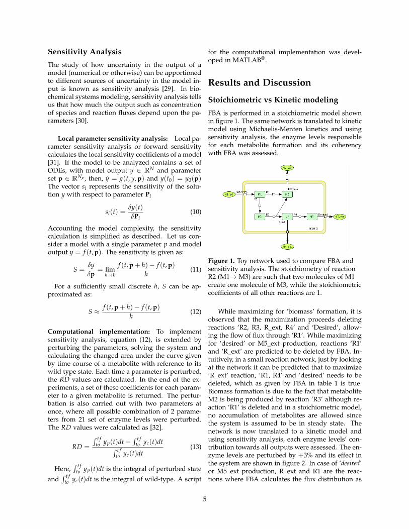
FBA is performed in a stoichiometric model shownin figure 1. The same network is translated to kineticmodel using Michaelis-Menten kinetics and usingsensitivity analysis, the enzyme levels responsiblefor each metabolite formation and its coherencywith FBA was assessed.

Figure 1. Toy network used to compare FBA andsensitivity analysis. The stoichiometry of reactionR2 (M1→ M3) are such that two molecules of M1create one molecule of M3, while the stoichiometriccoefficients of all other reactions are 1.

While maximizing for ‘biomass’ formation, it isobserved that the maximization proceeds deletingreactions ‘R2, R3, R_ext, R4’ and ‘Desired’, allow-ing the flow of flux through ‘R1’. While maximizingfor ‘desired’ or M5_ext production, reactions ‘R1’and ‘R_ext’ are predicted to be deleted by FBA. In-tuitively, in a small reaction network, just by lookingat the network it can be predicted that to maximize‘R_ext’ reaction, ‘R1, R4’ and ‘desired’ needs to bedeleted, which as given by FBA in table 1 is true.Biomass formation is due to the fact that metaboliteM2 is being produced by reaction ‘R3’ although re-action ‘R1’ is deleted and in a stoichiometric model,no accumulation of metabolites are allowed sincethe system is assumed to be in steady state. Thenetwork is now translated to a kinetic model andusing sensitivity analysis, each enzyme levels’ con-tribution towards all outputs were assessed. The en-zyme levels are perturbed by +3% and its effect inthe system are shown in figure 2. In case of ‘desired’or M5_ext production, R_ext and R1 are the reac-tions where FBA calculates the flux distribution as

5

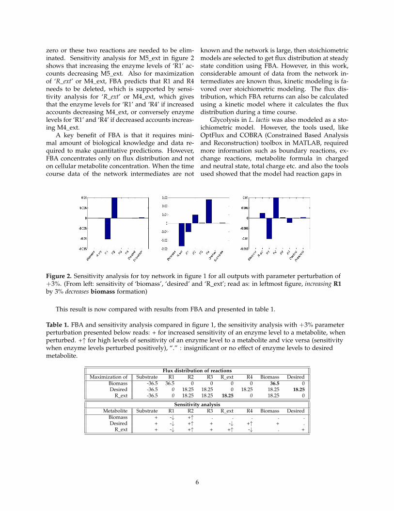
zero or these two reactions are needed to be elim-inated. Sensitivity analysis for M5_ext in figure 2shows that increasing the enzyme levels of ‘R1’ ac-counts decreasing M5_ext. Also for maximizationof ‘R_ext’ or M4_ext, FBA predicts that R1 and R4needs to be deleted, which is supported by sensi-tivity analysis for ‘R_ext’ or M4_ext, which givesthat the enzyme levels for ‘R1’ and ‘R4’ if increasedaccounts decreasing M4_ext, or conversely enzymelevels for ‘R1’ and ‘R4’ if decreased accounts increas-ing M4_ext.

A key benefit of FBA is that it requires mini-mal amount of biological knowledge and data re-quired to make quantitative predictions. However,FBA concentrates only on flux distribution and noton cellular metabolite concentration. When the timecourse data of the network intermediates are not

known and the network is large, then stoichiometricmodels are selected to get flux distribution at steadystate condition using FBA. However, in this work,considerable amount of data from the network in-termediates are known thus, kinetic modeling is fa-vored over stoichiometric modeling. The flux dis-tribution, which FBA returns can also be calculatedusing a kinetic model where it calculates the fluxdistribution during a time course.

Glycolysis in L. lactis was also modeled as a sto-ichiometric model. However, the tools used, likeOptFlux and COBRA (Constrained Based Analysisand Reconstruction) toolbox in MATLAB, requiredmore information such as boundary reactions, ex-change reactions, metabolite formula in chargedand neutral state, total charge etc. and also the toolsused showed that the model had reaction gaps in

Figure 2. Sensitivity analysis for toy network in figure 1 for all outputs with parameter perturbation of+3%. (From left: sensitivity of ‘biomass’, ‘desired’ and ‘R_ext’; read as: in leftmost figure, increasing R1by 3% decreases biomass formation)

This result is now compared with results from FBA and presented in table 1.

Table 1. FBA and sensitivity analysis compared in figure 1, the sensitivity analysis with +3% parameterperturbation presented below reads: + for increased sensitivity of an enzyme level to a metabolite, whenperturbed. +↑ for high levels of sensitivity of an enzyme level to a metabolite and vice versa (sensitivitywhen enzyme levels perturbed positively), “.” : insignificant or no effect of enzyme levels to desiredmetabolite.

Flux distribution of reactionsMaximization of Substrate R1 R2 R3 R_ext R4 Biomass Desired

Biomass -36.5 36.5 0 0 0 0 36.5 0Desired -36.5 0 18.25 18.25 0 18.25 18.25 18.25

R_ext -36.5 0 18.25 18.25 18.25 0 18.25 0

Sensitivity analysisMetabolite Substrate R1 R2 R3 R_ext R4 Biomass Desired

Biomass + -↓ +↑ . . . . .Desired + -↓ +↑ + -↓ +↑ + .

R_ext + -↓ +↑ + +↑ -↓ . +

6

its pathway. Since FBA is applied at steady state,any compound entering the system should alwaysexit. When this does not happens, there exists re-action gaps in the pathway which are to be filledto validate the steady state assumption. Since, aconsiderable amount of data, network structure andkinetic parameters were already available, stoichio-metric modeling is now left out and only kineticmodels are focused.

Approximated vs semi-mechanistic kinet-ics

Dynamic models of L. lactis from Voit et al., 2006 [2]and Vinga et al., 2010 [4] served as an initial modelto study glycolysis in L. lactis. It is known that PEPserves as a driving force to uptake any available glu-cose because of its involvement in PTS reaction andis also being converted to pyruvate, regulated byFBP. The regulation of glycolysis via PYK reactionhas been studied in [2]. The model used is adaptedand several things are manipulated.

Two system of kinetics, convenience kinetics andGMA system of kinetics are compared for the net-work topology obtained from Voit et al., 2006, [2].Within GMA and convenience kinetics, the time de-pendency of glucose decay is omitted in either ofmodeling approach and PGAPEP are consideredtwo different states which was not the case in [4].Few species are kept fixed with values for NAD =4.21, NADH = 3, ATP = 1, ADP = 5 and P = 1. Withavailable experimental data, the model parameterswere estimated. The fits were analyzed and boththe models were validated with 80 mM glucose im-pulse at time zero. Once both the systems are con-structed and validated, with (AICc), the two modelsare ranked.

With fixed concentration for NAD, NADH, ATP,ADP and P, the dynamics of the metabolites inthe pathway are defined properly, which was notthe case when these metabolites were consideredas state variables. Also, it is observed that thevalidation of the model follows the experimentaldata closely. The AICc gives: Convenience kinetics =339.337; GMA = 905.928, which concludes that whiletaking care of the network topology and accountingfor each variables that contributes to the involve-ment in other pathways, convenience kinetics equa-tions describes a model better than GMA system ofequations in terms of validation and AICc.

Model extension

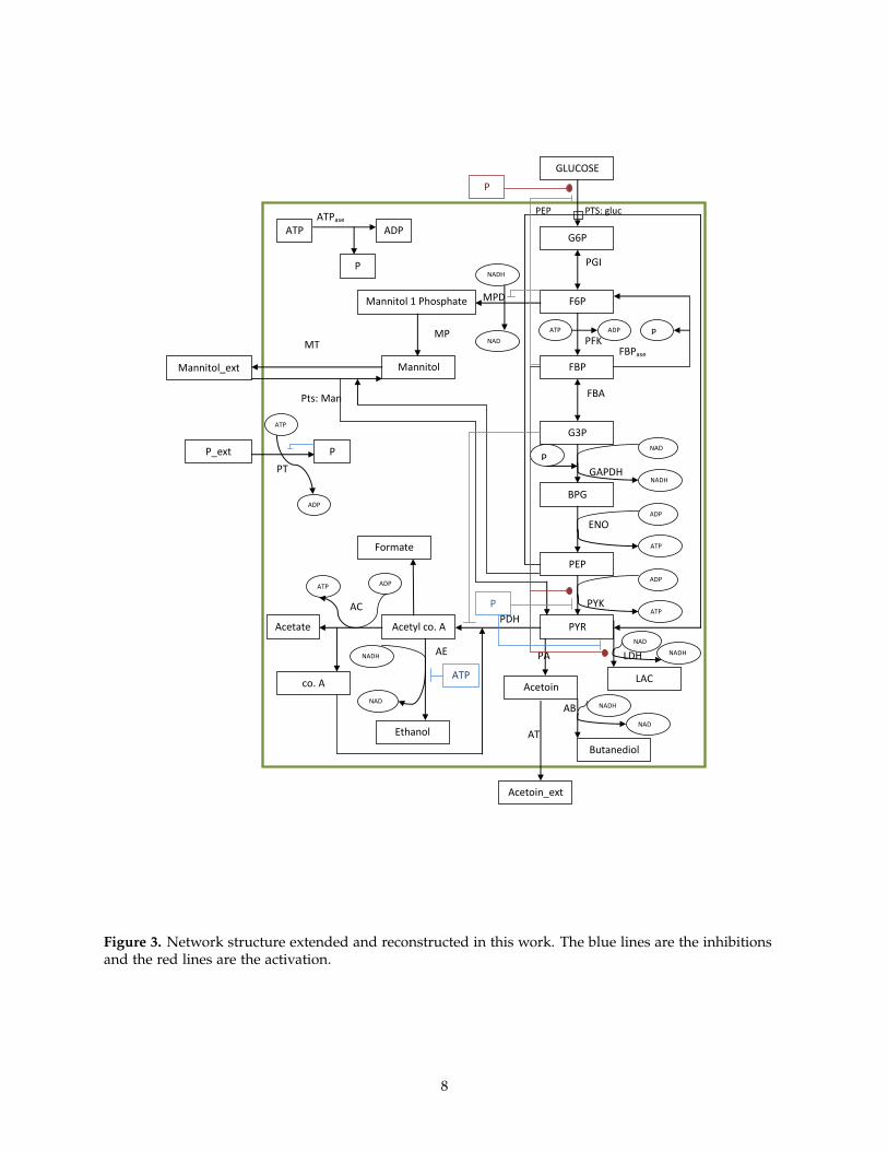
The network topology is extended to incorporateour metabolite of interest in the glycolytic pathway.An anaerobic glycolytic model in L. lactis, takingaccount into phosphate transfer reactions and ATPdegradation reactions is reconstructed. The net-work topology and initial parameters are obtainedfrom [1, 3, 33]. With few parameters unknown,these values are guessed such that the dynamics ofmetabolites (acetoin, butanediol, ethanol, formate)would stay low or resemble the production in Wildtype L. lactis. The model is then fitted with exper-imental data which although showed good fittingsand validations, did not accounted for transient dy-namics of acetoin and butanediol (not shown here).The parameters that were still not available for themodel to be reconstructed, which were guessed pre-viously, were now obtained from [34]. The exper-imental data for the analysis of the model fittingsand validation were available from Neves et al.,2005 [26]. The parameters are estimated using CO-PASI and a model with least objective function isselected for further analysis. The model topologyobtained is given in figure 3. Ten different runs ofparameter estimation were performed to get signifi-cant results. It can be seen that the best fitted model(black curve) in figure 4, follows the experimentaldata well except in the case of FBP, where it doesnot produces a bell shaped peak. Since the modelis trained using 40 mM data, inferring any conclu-sions without validating will give uncertain results.Thus, the model is now further validated changingthe glucose impulse (input).

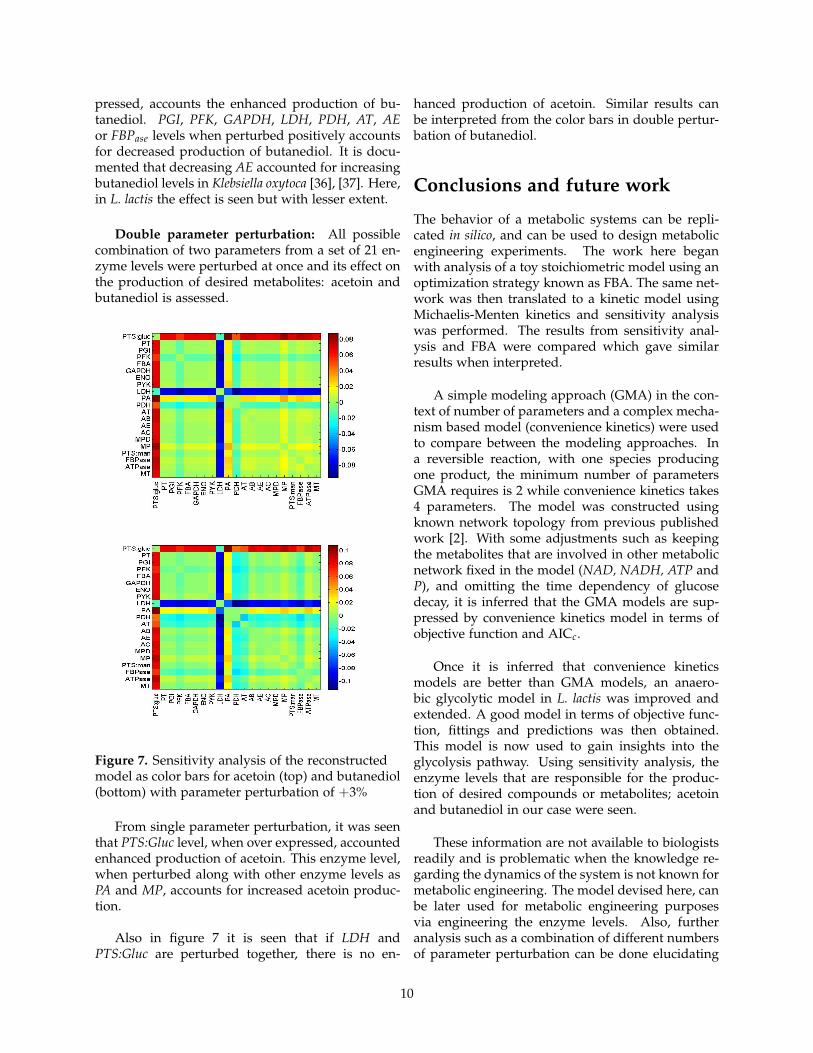
The trained model is now validated using 80mM glucose impulse at time zero. When comparingwith the the predictions made by the model againstthe experimental data, as given in figure 5, it canbe inferred that the response of the model for thechanged glucose impulse (input) follows the exper-imental data closely. When the predictions for FBP,ATP and P are observed, it can be said that someaspect in the models are lacking which leads to thedivergence of model predictions from experimentaldata. Considering that ATP and P are involved inentire metabolic network and not only limited to theglycolytic model studied here, it can be argued thatthis model provides a sufficient base for analyzingthe control points or reactions responsible for ourdesired metabolites, acetoin and butanediol. After agood predictive model in terms of validation, fittingand its overall characteristics is obtained, it is laterused for metabolic engineering purposes.

7

PEP PTS: gluc

PGI

PFK

FBA

GAPDH

ENO

PYK

PA LDH

AB

AT

GLUCOSE

G6P

F6P

FBP

G3P

BPG

PEP

PYR

LAC co. A

Butanediol

Acetyl co. A

Formate

Acetate

Ethanol

Acetoin

Mannitol 1 Phosphate

Mannitol

Acetoin_ext

Mannitol_ext

P_ext P

ATP

P

ADP

NAD

NADH

ATP ADP

P

ADP

ATP

ADP

ATP

NAD

NADH NADH

NAD

ATP ADP

NADH

NAD

NADH

NAD

P

ATP

P

PDH

AE

AC

MPD

MP MT

Pts: Man

ATP ADP

P

ATPase

PT

FBPase

Figure 3. Network structure extended and reconstructed in this work. The blue lines are the inhibitionsand the red lines are the activation.

8

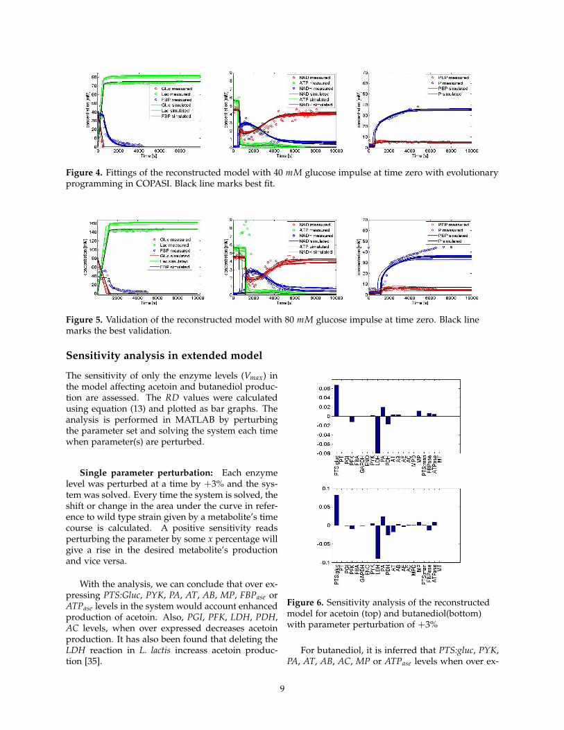
Figure 4. Fittings of the reconstructed model with 40 mM glucose impulse at time zero with evolutionaryprogramming in COPASI. Black line marks best fit.

Figure 5. Validation of the reconstructed model with 80 mM glucose impulse at time zero. Black linemarks the best validation.

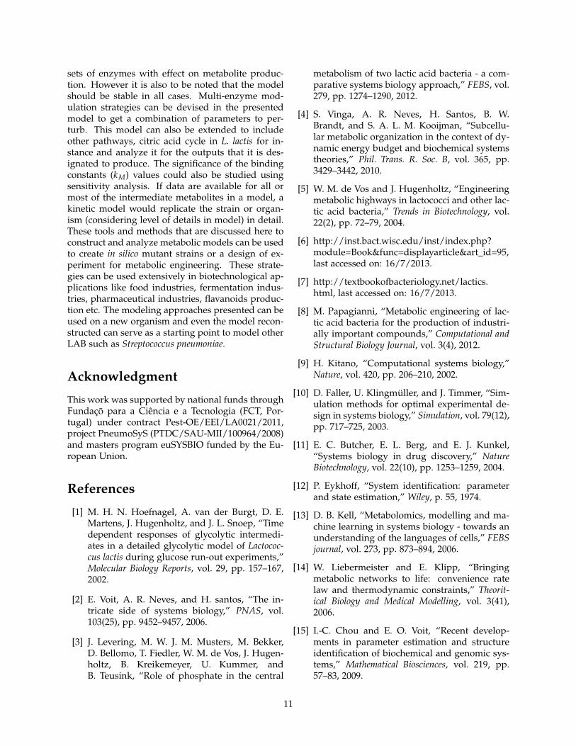
Sensitivity analysis in extended model

The sensitivity of only the enzyme levels (Vmax) inthe model affecting acetoin and butanediol produc-tion are assessed. The RD values were calculatedusing equation (13) and plotted as bar graphs. Theanalysis is performed in MATLAB by perturbingthe parameter set and solving the system each timewhen parameter(s) are perturbed.

Single parameter perturbation: Each enzymelevel was perturbed at a time by +3% and the sys-tem was solved. Every time the system is solved, theshift or change in the area under the curve in refer-ence to wild type strain given by a metabolite’s timecourse is calculated. A positive sensitivity readsperturbing the parameter by some x percentage willgive a rise in the desired metabolite’s productionand vice versa.

With the analysis, we can conclude that over ex-pressing PTS:Gluc, PYK, PA, AT, AB, MP, FBPase orATPase levels in the system would account enhancedproduction of acetoin. Also, PGI, PFK, LDH, PDH,AC levels, when over expressed decreases acetoinproduction. It has also been found that deleting theLDH reaction in L. lactis increass acetoin produc-tion [35].

Figure 6. Sensitivity analysis of the reconstructedmodel for acetoin (top) and butanediol(bottom)with parameter perturbation of +3%

For butanediol, it is inferred that PTS:gluc, PYK,PA, AT, AB, AC, MP or ATPase levels when over ex-

9

pressed, accounts the enhanced production of bu-tanediol. PGI, PFK, GAPDH, LDH, PDH, AT, AEor FBPase levels when perturbed positively accountsfor decreased production of butanediol. It is docu-mented that decreasing AE accounted for increasingbutanediol levels in Klebsiella oxytoca [36], [37]. Here,in L. lactis the effect is seen but with lesser extent.

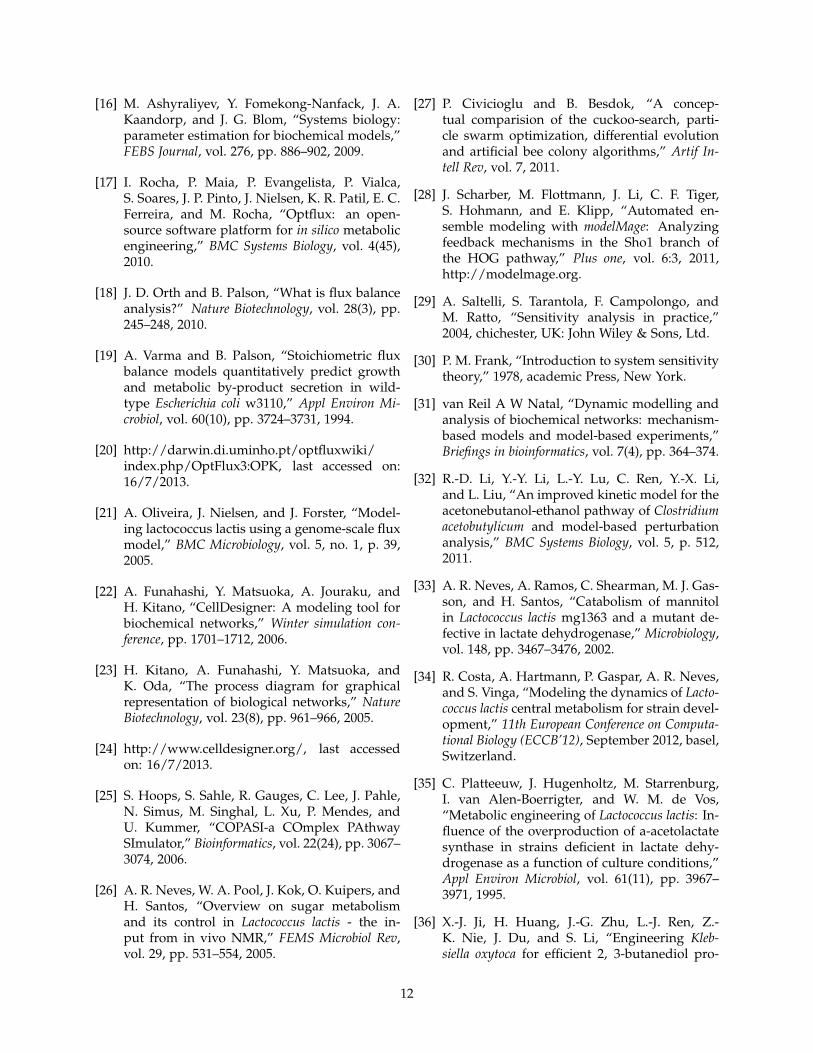
Double parameter perturbation: All possiblecombination of two parameters from a set of 21 en-zyme levels were perturbed at once and its effect onthe production of desired metabolites: acetoin andbutanediol is assessed.

Figure 7. Sensitivity analysis of the reconstructedmodel as color bars for acetoin (top) and butanediol(bottom) with parameter perturbation of +3%

From single parameter perturbation, it was seenthat PTS:Gluc level, when over expressed, accountedenhanced production of acetoin. This enzyme level,when perturbed along with other enzyme levels asPA and MP, accounts for increased acetoin produc-tion.

Also in figure 7 it is seen that if LDH andPTS:Gluc are perturbed together, there is no en-

hanced production of acetoin. Similar results canbe interpreted from the color bars in double pertur-bation of butanediol.

Conclusions and future work

The behavior of a metabolic systems can be repli-cated in silico, and can be used to design metabolicengineering experiments. The work here beganwith analysis of a toy stoichiometric model using anoptimization strategy known as FBA. The same net-work was then translated to a kinetic model usingMichaelis-Menten kinetics and sensitivity analysiswas performed. The results from sensitivity anal-ysis and FBA were compared which gave similarresults when interpreted.

A simple modeling approach (GMA) in the con-text of number of parameters and a complex mecha-nism based model (convenience kinetics) were usedto compare between the modeling approaches. Ina reversible reaction, with one species producingone product, the minimum number of parametersGMA requires is 2 while convenience kinetics takes4 parameters. The model was constructed usingknown network topology from previous publishedwork [2]. With some adjustments such as keepingthe metabolites that are involved in other metabolicnetwork fixed in the model (NAD, NADH, ATP andP), and omitting the time dependency of glucosedecay, it is inferred that the GMA models are sup-pressed by convenience kinetics model in terms ofobjective function and AICc.

Once it is inferred that convenience kineticsmodels are better than GMA models, an anaero-bic glycolytic model in L. lactis was improved andextended. A good model in terms of objective func-tion, fittings and predictions was then obtained.This model is now used to gain insights into theglycolysis pathway. Using sensitivity analysis, theenzyme levels that are responsible for the produc-tion of desired compounds or metabolites; acetoinand butanediol in our case were seen.

These information are not available to biologistsreadily and is problematic when the knowledge re-garding the dynamics of the system is not known formetabolic engineering. The model devised here, canbe later used for metabolic engineering purposesvia engineering the enzyme levels. Also, furtheranalysis such as a combination of different numbersof parameter perturbation can be done elucidating

10

sets of enzymes with effect on metabolite produc-tion. However it is also to be noted that the modelshould be stable in all cases. Multi-enzyme mod-ulation strategies can be devised in the presentedmodel to get a combination of parameters to per-turb. This model can also be extended to includeother pathways, citric acid cycle in L. lactis for in-stance and analyze it for the outputs that it is des-ignated to produce. The significance of the bindingconstants (kM) values could also be studied usingsensitivity analysis. If data are available for all ormost of the intermediate metabolites in a model, akinetic model would replicate the strain or organ-ism (considering level of details in model) in detail.These tools and methods that are discussed here toconstruct and analyze metabolic models can be usedto create in silico mutant strains or a design of ex-periment for metabolic engineering. These strate-gies can be used extensively in biotechnological ap-plications like food industries, fermentation indus-tries, pharmaceutical industries, flavanoids produc-tion etc. The modeling approaches presented can beused on a new organism and even the model recon-structed can serve as a starting point to model otherLAB such as Streptococcus pneumoniae.

Acknowledgment

This work was supported by national funds throughFundaçõ para a Ciência e a Tecnologia (FCT, Por-tugal) under contract Pest-OE/EEI/LA0021/2011,project PneumoSyS (PTDC/SAU-MII/100964/2008)and masters program euSYSBIO funded by the Eu-ropean Union.

References

[1] M. H. N. Hoefnagel, A. van der Burgt, D. E.Martens, J. Hugenholtz, and J. L. Snoep, “Timedependent responses of glycolytic intermedi-ates in a detailed glycolytic model of Lactococ-cus lactis during glucose run-out experiments,”Molecular Biology Reports, vol. 29, pp. 157–167,2002.

[2] E. Voit, A. R. Neves, and H. santos, “The in-tricate side of systems biology,” PNAS, vol.103(25), pp. 9452–9457, 2006.

[3] J. Levering, M. W. J. M. Musters, M. Bekker,D. Bellomo, T. Fiedler, W. M. de Vos, J. Hugen-holtz, B. Kreikemeyer, U. Kummer, andB. Teusink, “Role of phosphate in the central

metabolism of two lactic acid bacteria - a com-parative systems biology approach,” FEBS, vol.279, pp. 1274–1290, 2012.

[4] S. Vinga, A. R. Neves, H. Santos, B. W.Brandt, and S. A. L. M. Kooijman, “Subcellu-lar metabolic organization in the context of dy-namic energy budget and biochemical systemstheories,” Phil. Trans. R. Soc. B, vol. 365, pp.3429–3442, 2010.

[5] W. M. de Vos and J. Hugenholtz, “Engineeringmetabolic highways in lactococci and other lac-tic acid bacteria,” Trends in Biotechnology, vol.22(2), pp. 72–79, 2004.

[6] http://inst.bact.wisc.edu/inst/index.php?module=Book&func=displayarticle&art_id=95,last accessed on: 16/7/2013.

[7] http://textbookofbacteriology.net/lactics.html, last accessed on: 16/7/2013.

[8] M. Papagianni, “Metabolic engineering of lac-tic acid bacteria for the production of industri-ally important compounds,” Computational andStructural Biology Journal, vol. 3(4), 2012.

[9] H. Kitano, “Computational systems biology,”Nature, vol. 420, pp. 206–210, 2002.

[10] D. Faller, U. Klingmüller, and J. Timmer, “Sim-ulation methods for optimal experimental de-sign in systems biology,” Simulation, vol. 79(12),pp. 717–725, 2003.

[11] E. C. Butcher, E. L. Berg, and E. J. Kunkel,“Systems biology in drug discovery,” NatureBiotechnology, vol. 22(10), pp. 1253–1259, 2004.

[12] P. Eykhoff, “System identification: parameterand state estimation,” Wiley, p. 55, 1974.

[13] D. B. Kell, “Metabolomics, modelling and ma-chine learning in systems biology - towards anunderstanding of the languages of cells,” FEBSjournal, vol. 273, pp. 873–894, 2006.

[14] W. Liebermeister and E. Klipp, “Bringingmetabolic networks to life: convenience ratelaw and thermodynamic constraints,” Theorit-ical Biology and Medical Modelling, vol. 3(41),2006.

[15] I.-C. Chou and E. O. Voit, “Recent develop-ments in parameter estimation and structureidentification of biochemical and genomic sys-tems,” Mathematical Biosciences, vol. 219, pp.57–83, 2009.

11

[16] M. Ashyraliyev, Y. Fomekong-Nanfack, J. A.Kaandorp, and J. G. Blom, “Systems biology:parameter estimation for biochemical models,”FEBS Journal, vol. 276, pp. 886–902, 2009.

[17] I. Rocha, P. Maia, P. Evangelista, P. Vialca,S. Soares, J. P. Pinto, J. Nielsen, K. R. Patil, E. C.Ferreira, and M. Rocha, “Optflux: an open-source software platform for in silico metabolicengineering,” BMC Systems Biology, vol. 4(45),2010.

[18] J. D. Orth and B. Palson, “What is flux balanceanalysis?” Nature Biotechnology, vol. 28(3), pp.245–248, 2010.

[19] A. Varma and B. Palson, “Stoichiometric fluxbalance models quantitatively predict growthand metabolic by-product secretion in wild-type Escherichia coli w3110,” Appl Environ Mi-crobiol, vol. 60(10), pp. 3724–3731, 1994.

[20] http://darwin.di.uminho.pt/optfluxwiki/index.php/OptFlux3:OPK, last accessed on:16/7/2013.

[21] A. Oliveira, J. Nielsen, and J. Forster, “Model-ing lactococcus lactis using a genome-scale fluxmodel,” BMC Microbiology, vol. 5, no. 1, p. 39,2005.

[22] A. Funahashi, Y. Matsuoka, A. Jouraku, andH. Kitano, “CellDesigner: A modeling tool forbiochemical networks,” Winter simulation con-ference, pp. 1701–1712, 2006.

[23] H. Kitano, A. Funahashi, Y. Matsuoka, andK. Oda, “The process diagram for graphicalrepresentation of biological networks,” NatureBiotechnology, vol. 23(8), pp. 961–966, 2005.

[24] http://www.celldesigner.org/, last accessedon: 16/7/2013.

[25] S. Hoops, S. Sahle, R. Gauges, C. Lee, J. Pahle,N. Simus, M. Singhal, L. Xu, P. Mendes, andU. Kummer, “COPASI-a COmplex PAthwaySImulator,” Bioinformatics, vol. 22(24), pp. 3067–3074, 2006.

[26] A. R. Neves, W. A. Pool, J. Kok, O. Kuipers, andH. Santos, “Overview on sugar metabolismand its control in Lactococcus lactis - the in-put from in vivo NMR,” FEMS Microbiol Rev,vol. 29, pp. 531–554, 2005.

[27] P. Civicioglu and B. Besdok, “A concep-tual comparision of the cuckoo-search, parti-cle swarm optimization, differential evolutionand artificial bee colony algorithms,” Artif In-tell Rev, vol. 7, 2011.

[28] J. Scharber, M. Flottmann, J. Li, C. F. Tiger,S. Hohmann, and E. Klipp, “Automated en-semble modeling with modelMage: Analyzingfeedback mechanisms in the Sho1 branch ofthe HOG pathway,” Plus one, vol. 6:3, 2011,http://modelmage.org.

[29] A. Saltelli, S. Tarantola, F. Campolongo, andM. Ratto, “Sensitivity analysis in practice,”2004, chichester, UK: John Wiley & Sons, Ltd.

[30] P. M. Frank, “Introduction to system sensitivitytheory,” 1978, academic Press, New York.

[31] van Reil A W Natal, “Dynamic modelling andanalysis of biochemical networks: mechanism-based models and model-based experiments,”Briefings in bioinformatics, vol. 7(4), pp. 364–374.

[32] R.-D. Li, Y.-Y. Li, L.-Y. Lu, C. Ren, Y.-X. Li,and L. Liu, “An improved kinetic model for theacetonebutanol-ethanol pathway of Clostridiumacetobutylicum and model-based perturbationanalysis,” BMC Systems Biology, vol. 5, p. 512,2011.

[33] A. R. Neves, A. Ramos, C. Shearman, M. J. Gas-son, and H. Santos, “Catabolism of mannitolin Lactococcus lactis mg1363 and a mutant de-fective in lactate dehydrogenase,” Microbiology,vol. 148, pp. 3467–3476, 2002.

[34] R. Costa, A. Hartmann, P. Gaspar, A. R. Neves,and S. Vinga, “Modeling the dynamics of Lacto-coccus lactis central metabolism for strain devel-opment,” 11th European Conference on Computa-tional Biology (ECCB’12), September 2012, basel,Switzerland.

[35] C. Platteeuw, J. Hugenholtz, M. Starrenburg,I. van Alen-Boerrigter, and W. M. de Vos,“Metabolic engineering of Lactococcus lactis: In-fluence of the overproduction of a-acetolactatesynthase in strains deficient in lactate dehy-drogenase as a function of culture conditions,”Appl Environ Microbiol, vol. 61(11), pp. 3967–3971, 1995.

[36] X.-J. Ji, H. Huang, J.-G. Zhu, L.-J. Ren, Z.-K. Nie, J. Du, and S. Li, “Engineering Kleb-siella oxytoca for efficient 2, 3-butanediol pro-

12

duction through insertional inactivation of ac-etaldehyde dehydrogenase gene,” Appl Micro-biol Biotechnol, vol. 85, pp. 1751–1758, 2010.

[37] J. M. Park, H. Song, H. J. Lee, and D. Seung,

“Genome-scale reconstruction and in silicoanalysis of Klebsiella oxytoca for 2,3-butanediolproduction,” Microbial Cell Factories, vol. 12:20,2013.

13