Embed Size (px)
Citation preview

SERBIAN JOURNAL OF ELECTRICAL ENGINEERING
Vol. 4, No. 2, November 2007, 119-132
119
Dynamic Modeling and Simulation of an Induction
Motor with Adaptive Backstepping Design of an
Input-Output Feedback Linearization Controller in
Series Hybrid Electric Vehicle
Mehran Jalalifar1, Amir Farrokh Payam2,
Seyed Morteza Saghaeian Nezhad3, Hassan Moghbeli4
Abstract: In this paper using Adaptive backstepping approach an adaptive rotor
flux observer which provides stator and rotor resistances estimation simulta-neously for induction motor used in series hybrid electric vehicle is proposed.
The controller of induction motor (IM) is designed based on input-output
feedback linearization technique. Combining this controller with adaptive
backstepping observer the system is robust against rotor and stator resistances
uncertainties. In additional, mechanical components of a hybrid electric vehicle
are called from the Advanced Vehicle Simulator Software Library and then linked with the electric motor. Finally, a typical series hybrid electric vehicle is
modeled and investigated. Various tests, such as acceleration traversing ramp,
and fuel consumption and emission are performed on the proposed model of a
series hybrid vehicle. Computer simulation results obtained, confirm the validity
and performance of the proposed IM control approach using for series hybrid electric vehicle.
Keywords: Adaptive backstepping observer, Series electric vehicle.
1 Introduction
Nowadays the air pollution and economical issues are the major driving
forces in developing electric vehicles (EVs).
In recent years EVs and hybrid electric vehicles (HEVs) are the only
alternatives for a clean, efficient and environmentally friendly urban transporta-
tion system [1]. HEVs meet both consumer needs as well as car manufacturer
needs. They give the consumer the ability to use the car for long periods of time
1Islamic Azad University, Fereydan Branch, Esfahan, Iran; Email: [email protected] 2Dept. of Electrical & Computer Engineering, University of Tehran, Tehran 11365/4563, Iran; 3Dept. of Electrical & Computer Engineering, Isfahan University of Technology, Isfahan, Iran. 4Dept. of Electrical & Computer Engineering, Isfahan University of Technology, Isfahan, Iran; Email :[email protected]

M. Jalalifar, A.F. Payam, S.M.S. Nezhad, H. Moghbeli
120
without recharging. HEVs also take a giant step forward in meeting low
emission standards set by the Partnership for a New Generation of Vehicles.
Because of simple and rugged construction, low cast and maintenance, high
performance and sufficient starting torque and good ability of acceleration,
squirrel cage induction motor is a good candidate for EVs [2].
In this paper by using an input-output feedback linearization technique
combined with an adaptive backstepping observer in stator reference frame the
induction motor [3] using in series hybrid electric vehicle is controlled. One of
the best advantages of this control method is eliminating the flux sensor and
decreases the cost of controller in addition the control system is robust respect to
resistances variations and external load torque.
Advanced vehicle simulator (ADVISOR) provides the vehicle engineering
community with an easy-to-use, flexible, yet robust and supported analysis
package for advanced vehicle modeling. It is primarily used to quantify fuel
economy, the performance, and the emissions of vehicles that use alternative
technologies including fuel cells, batteries, electric motors, and ICE in hybrid
configurations. But the components in ADVISOR have been modeled simply
and only with static model to decrease the simulation time [4].
In this paper using MATLAB/SIMULINK software, dynamic modeling of
an induction motor that is used in series hybrid electric vehicle and controlled by
input-output feedback linearization method combined with adaptive
backstepping observer is investigated and then simulated separately by linking
the mechanical components for a series hybrid electric vehicle from the
ADVISOR software library. At the end, a typical HEV is modeled and investiga-
ted. Simulation results obtained show the IM and other components perfor-
mances for a typical city drive cycle.
2 The Performance of an Electric Vehicle
The first step in vehicle performance modeling is to write an equation for
the electric force. This is the force transmitted to the ground through the drive
wheels, and propelling the vehicle forward. This force must overcome the road
load and accelerate the vehicle as shown in Fig. 1 [5].
The rolling resistance is primarily due to the friction of the vehicle tires on
the road and can be written as:
roll rf f Mg= , (1)
where M is the vehicle mass, rf is the rolling resistance coefficient and g is
gravity acceleration.
The aerodynamic drag is due to the friction of the body of vehicle moving
through the air. The formula for this component is as in the following:

Dynamic Modeling and Simulation of an Induction Motor with…
121
21
2AD Df C AV= ξ , (2)
where ξ is the air mass density, and ,D
V C and A are the speed, the aerodynamic
coefficient, and the frontal area of the vehicle, respectively.
Fig. 1 – A summary of forces on a vehicle.
The gravity force due to the slope of the road can be expressed by:
singradef Mg= α , (3)
where α is the grade angle.
In addition to the forces shown in Fig. 3, another one is needed to provide
the linear acceleration of the vehicle given by:
d
dacc
Vf M M
t= α = . (4)
The propulsion system must now overcome the road loads and accelerate
the vehicle by the tractive force, tot
F , as follows:
tot roll AD grade accF f f f f= + + + . (5)
A typical road load characteristic as a function of the speed and mass of a
vehicle is shown in Fig. 2.
Fig. 2 – The road profile as a function of speed and mass of a vehicle ( 0α = ° ).

M. Jalalifar, A.F. Payam, S.M.S. Nezhad, H. Moghbeli
122
Wheels and axels convert tot
F and the speed of vehicle to torque and
angular speed requirements for the differential as follow [4]:
,wheel tot wheel wheel
wheel
VT F r
r= ω = , (6)
where wheel
T , wheelr , and
wheelω are the tractive torque, the radius, and the angular
velocity at the wheels, respectively.
The angular velocity and torque of the wheels are converted to motor rpm
and motor torque requirements using the gears ratio at differential and gearbox
as follows:
,
wheelm fd gb wheel m
fd gb
TG G T
G Gω = ω = , (7)
where fdG and gbG are respectively differential and gear box gears ratios.
A series HEV consists of two major group components as shown in Fig. 3:
- Mechanical components (engine, wheels, axels and transmission box) and
- Electrical components (batteries and electric motor).
Fig. 3 – A series hybrid electric vehicle.
3 Electric Motor
Due to the simple and rugged construction, low cast and maintenance, high
performance and sufficient starting torque and good ability of acceleration,
squirrel cage induction motor is one of the well suited motors for the electric
propulsion systems [6]. In this section first modeling of the induction motor in

Dynamic Modeling and Simulation of an Induction Motor with…
123
stator fixed reference frame and then designing an input-output controller
combined with adaptive backstepping observer for IM [3] is investigated.
A. Input-Output Feedback linearization Controller Design
The square of rotor flux amplitude is taken as the first output of the
controlled system
2 2 2
1
2 2
1 1 1
,
,
ra rb r
r
d r r
y
e y y
= ψ +ψ = ψ
= − = ψ −ψ )8(
where r
rψ is the reference signal for rotor flux amplitude.
Differentiating 1y so much inputs ( , )
sa sbu u appear in our equations,
1
2 2r r r r
ra ra sa rb rb sb
r r r r
R R R Ry Mi Mi
L L L L
⎛ ⎞ ⎛ ⎞= ψ − ψ + + ψ − ψ +⎜ ⎟ ⎜ ⎟
⎝ ⎠ ⎝ ⎠� . (9)
Then
1
2 2
2 2
4
2
4 2 .
r r r
ra ra sa
r r r
r r s sar r
ra ra sa
r s r s r s
r r r r
rb rb sb rb
r r r r
R R Ry Mi
L L L
M R L R uR MRM i
L L L L L L
R R R RMi M
L L L L
⎛ ⎞= − ψ − ψ + +⎜ ⎟
⎝ ⎠
⎛ ⎞++ ψ ψ − + −⎜ ⎟
σ σ σ⎝ ⎠
⎛ ⎞− ψ ψ + + ψ⎜ ⎟
⎝ ⎠
��
(10)
If 1e dynamic force to be
11 1 12 1 13 10k e k e k e+ + =�� � ,
we have
11 1 1 12 1 1 13 1 1( ) ( ) ( ) 0
d d dk y y k y y k y y− + − + − =�� �� � � ,
( )
1312
1 1 1 1 1 1
11 11
2 213 12
11 11
2
( ) ( )
( ) 2
2 2 2 .
d d d
r r r
r r ra ra sa
r r
r r r r rr r
rb rb sb r r r r r
r r
kky y y y y y
k k
k k R RMi
k k L L
R RMi
L L
= − + − + =
⎧ ⎛ ⎞⎪= ψ −ψ − ψ − ψ + +⎨ ⎜ ⎟
⎪ ⎝ ⎠⎩
⎫⎛ ⎞⎪+ ψ − ψ + − ψ ψ + ψ +ψ ψ⎬⎜ ⎟
⎪⎝ ⎠⎭
�� � � ��
� � ��
(11)
Now the motor developed electromagnetic torque is considered as the
second output

M. Jalalifar, A.F. Payam, S.M.S. Nezhad, H. Moghbeli
124
2
2 2 2
( )2
p
ra sb rb sa
r
r
d
n My te i i
L
e y y te te
= = ψ −ψ
= − = −
)12(
where r
te is the reference signal for developed electromagnetic torque.
Time derivative of 2y is:
2 2
2 2
2 2
2
2
.
p p r r s sb
ra ra sb
r s r s r s
p r r s sarsb ra p rb rb rb sa
r s r s r s
rsa rb p ra
r
n M n M M R L R uy i
L L L L L L
n M M R L R uRi n i
L L L L L L
Ri n
L
⎧ ⎛ ⎞+⎪= ψ − ωψ − + +⎨ ⎜ ⎟σ σ σ⎪ ⎝ ⎠⎩
⎛ ⎞⎛ ⎞ ++ − ψ − ωψ −ψ ωψ − + −⎜ ⎟⎜ ⎟ σ σ σ⎝ ⎠ ⎝ ⎠
⎫⎛ ⎞⎪− − ψ + ωψ ⎬⎜ ⎟⎪⎝ ⎠⎭
�
(13)
By setting 2e dynamic as
21 2 22 20k e k e+ =� ,
we have
21 2 2 22 2 2( ) ( ) 0
d dk y y k y y− + − =� � ,
22 22
2 2 2 2
21 21
( ) ( )r r
d d
k ky y y y te te te
k k= − + = − + �� � . (14)
Setting right side of (13) equal to right side of (14), another equation for
inputs is achieved
2 2
2
2 2
2
22
21
2
( ) .
p p r r s sb
ra ra sb
r s r s r s
p r r s sarsb ra p rb rb rb sa
r s r s r s
r rrsa rb p ra
r
n M n M M R L R ui
L L L L L L
n M M R L R uRi n i
L L L L L L
R ki n te te te
L k
⎧ ⎛ ⎞+⎪ψ − ωψ − + +⎨ ⎜ ⎟σ σ σ⎪ ⎝ ⎠⎩
⎛ ⎞⎛ ⎞ ++ − ψ − ωψ −ψ ωψ − + −⎜ ⎟⎜ ⎟ σ σ σ⎝ ⎠ ⎝ ⎠
⎫⎛ ⎞⎪− − ψ + ωψ = − +⎬⎜ ⎟⎪⎝ ⎠⎭
�
(15)
Now, from system of two equations, (6 and 10), inputs ( , )sa sb
u u are found.
To proof the stability of proposed controller, note that according to
dynamics of1 2, ,e e if initially
1 1(0) (0) 0e e= =� and also
2(0) 0,e = then
1 2( ), ( ) 0, 0,e t e t t≡ ∀ ≥ perfect tracking is achieved; otherwise,
1 2( ), ( )e t e t
converges to zero exponentially [7].

Dynamic Modeling and Simulation of an Induction Motor with…
125
B. Adaptive Backstepping Observer Design
Stator current is measurable and is taken as output:
,a sa b sby i y i= = . (16)
The prediction model for the backstepping observer is chosen to be
2 2
2 2
2 2
2 2
ˆ ˆˆ ˆ ˆ ,
ˆ ˆˆ ˆ ˆ ,
ˆ ˆˆ 1ˆ ˆ ˆ ,
ˆ ˆˆ 1ˆ ˆ ˆ
r rra ra p rb a
r r
r rrb rb p ra b
r r
p r r srsa ra rb a sa a
s r s r s r s
p r r srsb rb ra b sb
s r s r s r s
R Rp n My
L L
R Rp n My
L L
n M M R L RMRpi y u v
L L L L L L L
n M M R L RMRpi y u v
L L L L L L L
ψ = − ψ − ωψ +
ψ = − ψ + ωψ +
+= ψ + ωψ − + +σ σ σ σ
+= ψ − ωψ − + +σ σ σ σ
,b
(17)
where p is the differential operator and ,a bv v are the control input to be
designed by the backstepping method.
The dynamical equations for the prediction errors are
2 2
2 2 2
2 2
ˆ,
ˆ,
ˆ,
ˆ
r r rra ra ra p rb a
r r r
r r rrb rb rb p ra b
r r r
p r r sr rsa ra ra rb a a
s r s r s r s r
pr rsb rb rb
s r s r s
R R Rp n My
L L L
R R Rp n My
L L L
n M M R L RMR MRpi y v
L L L L L L L L
n MMR MRpi
L L L L L
ψ = − ψ − ψ − ωψ +
ψ = − ψ − ψ + ωψ +
+= ψ + ψ + ωψ − +σ σ σ σ
= ψ + ψ −σ σ σ
� �
� � �
� �
� � �
� ��� � �
�� �
�
�
2 2
2,
,
,
r r sra b b
r s r
saa
sbb
M R L Ry v
L L L
y i
y i
+ωψ − +
σ
=
=
� �
�
�
�
(18)
where
ˆˆ ˆ, , ,
ˆ ˆˆ , , .
ra ra ra rb rb rb sa sa sa
sb sb sb s s s r r r
i i i
i i i R R R R R R
ψ =ψ −ψ ψ = ψ −ψ = −
= − = − = −
�� �
� �� (19)
The first step in the backstepping strategy is to design a stable controller for
the integral of the prediction errors � �,
a by y using ,sa sbi i� � as virtual control

M. Jalalifar, A.F. Payam, S.M.S. Nezhad, H. Moghbeli
126
variables with stabilizing functions ,a b
φ φ which is reference for virtual
variables. The integral of the prediction errors � �,a bx x are
� �, .a sa b sbpx i px i= =
� � (20)
Adding and subtracting ,a b
φ φ to above equations
� � � �
� �
1 1
1 1
, ,
, ,
, .
a a b ba b
sa sba a b b
a ba b
px z c x px z c x
z i z i
c x c x
= − = −
= − φ = − φ
φ = − φ = −
� � (21)
The second step in the backstepping strategy is the control of
� �1 1
,sa a sb ba bz i c x z i c x= + = +
� � . (22)
Taking the derivative of az and
bz ,
2 2
12 2 2
2 2
12 2 2
ˆ,
ˆ
p r r sr ra ra ra rb a a sa
s r s r s r s r
p r r sr rb rb rb ra b b sb
s r s r s r s r
n M M R L RMR MRz y v c i
L L L L L L L L
n M M R L RMR MRz y v c i
L L L L L L L L
+= ψ + ψ + ωψ − + +σ σ σ σ
+= ψ + ψ − ωψ − + +σ σ σ σ
� ���� ��
� ���� ��
(23)
and selecting following control inputs
1 22
1 22
ˆ,
ˆ,
pra ra rb sa a a
s r s r
prb rb ra sb b b
s r s r
n MMRv c i c z x
L L L L
n MMRv c i c z x
L L L L
= − ψ − ωψ − − −σ σ
= − ψ + ωψ − − −σ σ
�� � �
�� � �
(24)
yields
2 2
22 2
2 2
22 2
,
,
r r sr
a ra a a a
s r s r
r r sr
b rb b b b
s r s r
M R L RMRz y c z x
L L L L
M R L RMRz y c z x
L L L L
+= ψ − − −σ σ
+= ψ − − −σ σ
� ��
��
� ��
��
(25)
where 1c and
2c are positive constant design parameters.
Stability analysis of observer is done by the following Lyapunov candidate:
2 2 2 2 2 2 2 21 1 1
2a b a b ra rb s r
s r
V x x z z R R⎧ ⎫⎪
= + + + + ψ + ψ + +⎨ ⎬γ γ⎪ ⎭⎩
� �� �� � . (26)
Derivating V along the dynamics of (18, 21 and 25) yields

Dynamic Modeling and Simulation of an Induction Motor with…
127
2 2 2 2 2 2
1 1 2 2
2 2
2 2
2 2
2 2 2 2
ˆ ˆ
1
1
r r
a b a b ra rb
r r
a r b r s
s a b
s r s r s
a a b b ra ra
r ra a rb b
s r s r s r s r r
rb rb
a ra b rb
r r r
R RV c x c x c z c z
L L
z L z L dRR y y
L L L L dt
z M M z z M M zR y y
L L L L L L L L L
M My y
L L L
= − − − − − ψ − ψ
⎧ ⎫+ − − +⎨ ⎬
σ σ γ⎩ ⎭
⎧ ψ ψ+ ψ − + ψ − −⎨
σ σ σ σ⎩
ψ ψ+ ψ − + ψ +
γ
� � �� �
��
��
�� � .
r
r
dR
dt
⎫⎬⎭
�
(27)
By selecting following adaptation laws
2 2
2 2
2 2
2 2 2 2
,
s a r b r
s a b
s r s r
a a b br
r ra a rb b
s r s r s r s r
ra ra rb rb
a ra b rb
r r r r
dR z L z Ly y
dt L L L L
z M M z z M M zdRy y
dt L L L L L L L L
M My y
L L L L
⎧ ⎫= γ +⎨ ⎬
σ σ⎩ ⎭
⎧= γ − ψ + − ψ +⎨
σ σ σ σ⎩
⎫ψ ψ ψ ψ+ − ψ + − ψ ⎬
⎭
�
�
� �� �
(28)
we have 0V <� outside the equilibrium point
( , , , , , )a b a b ra rbx x z z ψ ψ =� �� � (0,0,0,0,0,0).
Based on the Barbalat’s Lemma, we can obtain , , ,a b ax x z� � , ,
b ra rbz ψ ψ� � will
converge to zero as t →∞ . Therefore, the proposed observer is stable, even if
parametric uncertainties exist [8]. The block diagram of the proposed controller
is given in Fig. 4.
PI
Controller
Input-Output
FeedbeackLineariztion
Controller
Adaptive Backstepping
Obsrever
ParkTransformation
IM
r
rΨ
r
te
,ra
� rb�
sR�
rR�
ω
sau
sbu
sAu
sCu
sBu
sAi
sBi sC
i
r
ω
+-
Fig. 4 – Block diagram of proposed controller.

M. Jalalifar, A.F. Payam, S.M.S. Nezhad, H. Moghbeli
128
4 Battery Modeling
The battery considered in this paper is of the NiMH type for which a simple
model is assumed. Therefore, a simplified version of the complex battery model
reported in [9] is used.
5 Simulation Results
Simulation results presented in this section, focus on the dynamic behavior
of IM and the battery of the vehicle. First the system is simulated for
ECE+EUDC test cycle. This cycle is used for emission certification of light duty
vehicles in Europe. Due to the electric motor has been modeled dynamically in
SIMULINK. The data for IM and EV is in the appendix.
Fig. 5 shows the simulation block diagram.
Baterries
Set
Electric
Motor
Power
Converter
Transmission System
and Differentional
GeneratorPower
Converter
Diesel
EngineWheel
Controller Wheel
Electric Energy
FlowElectric Energy
Flow
Electric Signal
Flow
Fig. 5 – Simulation block diagram.
The drive cycle gives the required vehicle speed then the torque and speed
requested from the electric motor. The current drawn from IM power supply
shows the battery performance. The dynamic behavior of the IM in the
ECE+EUDC drive cycle is shown in Figs. 6(a) and 6(d). Fig. 6(a) shows the
ECE drive cycle. Figs. 6(c) and 6(d) show the IM torque and average torque.
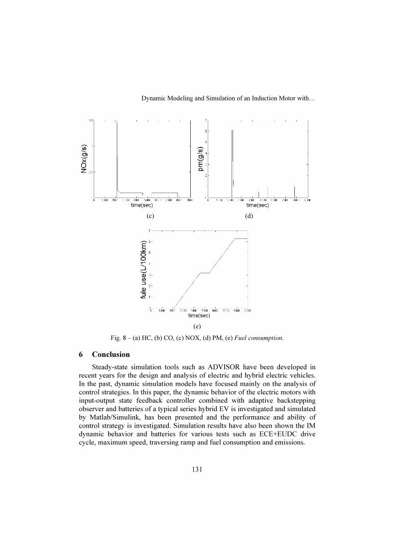
Finally, the system is simulated for fuel consumption and emissions test.
The results obtained are shown in Fig. 7 and Fig. 8. Fig. 7 shows the fuel consu-
mption and emissions of diesel engine when the motor is hot at the start of test,
and Fig. 8 shows the results when the engine is cool at the start of test. It is

Dynamic Modeling and Simulation of an Induction Motor with…
129
obvious that when the engine is cool, fuel consumption and emissions is
increases respect to the engine is hot.
(a) (b)
(c) (d)
Fig. 6 – (a) ECE drive cycle, (b) Vehicle speed, (c) Average torque, (d) IM torque.
(a) (b)
Fig. 7 – (a) HC, (b) CO consumption.

M. Jalalifar, A.F. Payam, S.M.S. Nezhad, H. Moghbeli
130
(c) (d)
(e)
Fig. 7 – (c) NOX, (d) PM, (e) Fuel consumption.
(a) (b)
Fig. 8 – (a) HC, (b) CO consumption.
Dynamic Modeling and Simulation of an Induction Motor with…
131
(c) (d)
(e)
Fig. 8 – (a) HC, (b) CO, (c) NOX, (d) PM, (e) Fuel consumption.
6 Conclusion
Steady-state simulation tools such as ADVISOR have been developed in
recent years for the design and analysis of electric and hybrid electric vehicles.
In the past, dynamic simulation models have focused mainly on the analysis of
control strategies. In this paper, the dynamic behavior of the electric motors with
input-output state feedback controller combined with adaptive backstepping
observer and batteries of a typical series hybrid EV is investigated and simulated
by Matlab/Simulink, has been presented and the performance and ability of
control strategy is investigated. Simulation results have also been shown the IM
dynamic behavior and batteries for various tests such as ECE+EUDC drive
cycle, maximum speed, traversing ramp and fuel consumption and emissions.

M. Jalalifar, A.F. Payam, S.M.S. Nezhad, H. Moghbeli
132
7 Appendix
A. EV Data:
Vehicle total mass of 8200 kg; Air drag coefficient of 0.79; Rolling
resistance coefficient of 0.008; Wheel radius of 0.41 m; Level ground; Zero head
wind.
B. The IM Parameters:
nP 75[kW]
mX 1.95[ ]Ω
maxP 189[kW]
lsX 0.06[ ]Ω
f 60[Hz] lr
X ′ 0.06[ ]Ω
nT 209[Nm]
sn 3600[r .p.m]
maxT 520[Nm] J 1.2 2[kgm ]
sR 0.02[ ]Ω P 2
rR′ 0.01[ ]Ω
8 References
[1] M. Ehsani, K.M. Rahman, H.A. Toliyat: Propulsion System Design of Electric and Hybrid
Vehicle, IEEE Tran. On industrial Electronics, Vol. 44, No.1, February 1997.
[2] http://www.ott.doe.gov/hev/
[3] R. Yazdanpanah, A. Farrokh Payam: Direct Torque Control of An Induction Motor Drive
Based on Input-Output Feedback Linearization Using Adaptive Backstepping Flux Observer,
Proc. 2006 AIESP Conf., Madeira, Portugal.
[4] T. Markel, A. Brooker, T. Hendricks, V. Johnson, K. Kelly, B. Kramer, M. O' Keefe, S.
Sprik, K. Wipke: ADVISOR: A Systems Analysis Tool for Advanced Vehicle Modeling,
ELSEVIER Journal of Power Sources 110, (2002), pp. 255-266.
[5] Electric Vehicle Technology Explained , Editted by James Larminie, and John Lowry, John
Wiley, England, 2003.
[6] A. Rahide: Vector Control of Induction Motor Using Neural Network in Electric Vehicle,
Scientific Report, IUST, 2000.
[7] R. Marino, S. Peresada, P. Valigi: Adaptive Input-Output Linearization Control of Induction
Motors, IEEE Trans. Automatic Cont., Vol. 38, No. 2, pp. 208-220, Feb. 1993.
[8] Applied Nonlinear Control , Editted by J. E. Slotine, Prentice-Hall International Inc.
[9] S. Sadeghi, J. Milimonfared, M. Mirsalim, M. Jalalifar: Dynamic Modeling and Simulation
of a Switched Reluctance Motor in Electric Vehicle, in Proc., 2006 ICIEA Conf.


![5 Dynamic Modeling[1]](https://img.pdfslide.net/doc/110x75/577cc7241a28aba711a01adb/5-dynamic-modeling1.jpg)