DYNAMIC MODELING FOR STRUCTURES

WITH BOLTED JOINTS

By

Asal Kharazi Kalajahi

Thesis

Submitted to the Faculty of Mechanical Engineering

At Politecnico di Torino

for the degree of

MASTER OF SCIENCE

in

Mechanical Engineering

March-April 2019

2

CONTENTS Introduction .................................................................................................................................................. 3

What is a jointed structure? ..................................................................................................................... 3

Modeling of Mechanical Joints ................................................................................................................. 3

Commercial codes ..................................................................................................................................... 4

What is a common joint? .......................................................................................................................... 4

Historical Development ............................................................................................................................ 4

The benefit of designing structures with Joints ........................................................................................ 6

Perspectives for the Economics of Jointed Structures: ........................................................................ 6

Experimental Techniques for Studying Energy Dissipation Mechanics .................................................... 6

Round Robin Systems............................................................................................................................ 6

Damping .................................................................................................................................................. 20

The damping sites within a bolted joint ............................................................................................. 20

Considerations for Measurements of Jointed Structures ....................................................................... 21

Effects of Experimental Setup ............................................................................................................. 21

Best Practices for Experiments on Jointed Systems ........................................................................... 21

Introduction of constitutive models ........................................................................................................... 22

Modeling Considerations ........................................................................................................................ 22

Friction Models ....................................................................................................................................... 22

1.Velocity-Based Models ..................................................................................................................... 22

2. State-Based Models ........................................................................................................................ 23

Test case: Two Cantilevered Beams ............................................................................................................ 26

RESULTS .................................................................................................................................................. 27

Case study Beam 1 .............................................................................................................................. 27

Case Study Beam 2 .............................................................................................................................. 29

Case Study of Two Cantilever Beams Assembly with four bolts ......................................................... 32

Iwan Model Introduction ............................................................................................................................ 37

Four-Parameter Iwan Model .................................................................................................................. 38

Extended Iwan-Type Models: Five-Parameter Iwan-Type Model .......................................................... 42

The Next Generation of Joints Research ................................................................................................. 44

On Numerical Modeling ...................................................................................................................... 44

3

INTRODUCTION

What is a jointed structure? The primary function of a joint in an engineering structure is to connect, usually stiffly, two (or more)

separate substructures. Joints introduce two features to a structure: amplitude dependent stiffness and

amplitude dependent damping. The amplitude dependent stiffness can be predicted reasonably well (to

within 10%); however, the amplitude dependent damping is still beyond predictive capabilities. The analysis

of jointed structures consists of two principle parts: the deterministic/linear substructures that can be

readily modeled and analyzed with existing techniques, and the often unpredictable assembly of a jointed

structure that exhibits emergent behavior not observed in the deterministic substructures.

In joint mechanics, contrary to Hayek’s assertion, it is quite possible that the knowledge for fully

characterizing a joint will be prohibitively difficult to obtain for modeling purposes. From experimental and

numerical evidence, the nonlinearities introduced by joints seem to be dependent upon qualities

introduced by the manufacturing process that cannot be measured.

Modeling of Mechanical Joints As of yet, there is no consensus for the best practice of modeling a jointed connection. In academia, there

are many new techniques that are often in their infancy: significant validation and verification work is

needed in addition to making them usable and efficient.

The analysis is divided into three stages:

1. Nonlinear Static Solve

2. High Fidelity Contact Interface Modeling

3. Dynamic Analysis

The first step, the nonlinear static solve, is used to determine which nodes in the interface are stuck

together, and which nodes are not expected to be in contact.

In the second step, the problem is reduced slightly by assuming that nodes that are out of contact will

remain out of contact during the analysis. The remaining nodes are considered to be potentially slipping.

Though under certain circumstances these could be divided into stuck and slipping, in which case the stuck

nodes just need to be attached with linear springs.

The third step is the dynamic analysis. Once the contact interface has been prescribed, the next challenge

is determining the quantity of interest. For frequency responses, harmonic balance-based simulations are

preferable as the frequency response will exhibit nonlinearities dependent up on the excitation amplitude.

4

Commercial codes Large number of node-to-node contacts will need to be specified for high fidelity finite element commercial

codes. Recent advances by commercial finite element packages exhibit capabilities to minimize the burden

placed on the user for this modeling. some successful commercial codes to mention are:

The use of ADAMS, a multibody dynamics code, with flexible bodies modeled in NASTRAN (Hopkins

and Heitmann 2016). This approach is very efficient for macroslip, but not amenable for microslip

applications.

The use of ANSYS to introduce bolts to geometrically flat surfaces.

The use of ABAQUS, Hyperworks, or other codes with node-to-node contact and preloaded bolts.

The goal of joint research is, and will continue to be for the foreseeable future, the development of a

predictive model for the interfacial dissipation and stiffness of a joint.

What is a common joint? It is defined as the mating of two components through a bolted connection. This simple geometry is used

in wind turbine structure and cylindrical flanges or seals. The lap joint is the most common type of interface

found in built-up structures. Throughout all of the perturbations of the simple lap joint geometry, the

common features are one (or more) bolts used to hold together two (or more) surfaces under a normal

compressive load due to the bolt.

In general, lap joints are designed such that the compressive load is sufficiently high to prevent the massive

relative motion of the two components. Movement along the interface between the two components is

generally isolated and not complete throughout. This isolated movement is termed microslip and

specifically refers to the relative motion between the two interfaces that only occurs over part of the

interface while the rest of the interface exhibits no relative motion. Microslip is expected to first occur away

from the bolt locations. As the excitation magnitude is increased, the domain of microslip will increase until

the entire interface exhibits relative (sliding) motion, which is macroslip.

In designing a lap joint, the primary function is to connect stiffy two components. This task is relatively

straightforward, and there are multiple handbooks that detail selections of materials, bolts, and preload to

ensure that the primary function of a joint is met.

Historical Development Taking into consider the immense nature of the challenge of developing a predictive model of friction, the

American Society of Mechanical Engineers (ASME) Research Committee on the Mechanics of Jointed

Structures was formed to develop collaborations and to advance the state of the art for modeling structures

with jointed interfaces. As part of the collaborations established by this community, a series of workshops

have been conducted over the past eight years (Segalman et al.2007, 2010; Starr et al.2013). At the

5

conclusion of these workshops, the last activity is to summarize the discussion and to formulate a series of

challenges and action items.

From the first workshop ( Segalman et al. 2007), three challenges were identified:

1.The experimental measurements of joint properties

2.Interface physics

3.Multi-scale modeling

These three challenges represent an ambitious set of goals that have persisted into the outcomes of the

subsequent two workshops. One direct consequence of this workshop was the publication of the Joints

Handbook (Segalman et al.2009), which methodically detailed Sandia National Laboratories’ approach to

experimental measurements and numerical modeling of joints in structures. This handbook has since been

used extensively by the joints community.

The second workshop (Segalman et al. 2010) built on the set of challenges formulated during the first

workshop and defined eleven new challenges:

1. Round-robin/benchmark exercise for hysteresis measurements

2. Round-robin/benchmark exercise for the measurement and prediction of dissipation in standard

joints

3. Repeatability and variability

4. Framework for multi-scale modeling

5. Strategy for uncertainty and nonlinearity

6. Methodology to quantify the cost benefits of improved joints designs

7. Universally accepted physical theory of friction

8. Complex loading strategies

9. Measurement of spatial distribution of key physical parameters

10. How to include surface chemistry?

11. Eventual implementation of prediction methods in commercial numerical codes

Inherent in this set of eleven challenges are the same three themes from the first workshop: experimentally

measuring joint properties, the physics of the joint interface, and modeling techniques to bridge the gap

between reality and simulation. The modeling techniques can be subdivided into three overarching classes:

multi-scale frameworks, uncertainty quantification and propagation, and numerical methods to simulate a

jointed system efficiently and accurately. The three themes are seen again with the challenges developed

at third workshop.

From the third workshop, seven challenges were defined after a mini-workshop held the following year

revisited them. These challenges are:

1. Round-robin/benchmark exercise for hysteresis measurements

2. Round-robin/benchmark exercise for measurement and prediction of dissipation in standard

3. The economics of jointed structures

4. Defining the mechanism of friction

5. Epistemic and aleatoric uncertainty in modeling and measurements

6. Derivation of constitutive equations based on physical parameters

7. Eventual implementation and integration of prediction methods in finite element codes

6

Following the third workshop and before the mini-workshop which was held in Portland, five other

challenges existed: modeling nonmetallic interfaces, multi-scale modeling framework, epistemic and

aleatoric modeling, definition of variability and uncertainty, and time varying model parameters, modeling

and experimental “surface chemistry”. The challenge on modeling nonmetallic interfaces was postponed

in order to focus our efforts on metallic interfaces first before considering a second class of interfaces.

The benefit of designing structures with Joints

Engineers and designers can directly reduce the cost by reducing the number of man-hour needed to design

a system with the use of joints in the models and the handbooks with easily digested metrics for how a

specific joint performed.

One goal of joints research is to be able to use joints to monitor the state of a structure actively. With this

capability, it would be possible to plan a repair cycle optimally for a given structure, and to then use the

joints as an early warning sign to help avoid a structural failure. Thus having joints as a means of detection

of potential problems could introduce significant cost savings. This is particularly relevant to the aerospace

industry.

Perspectives for the Economics of Jointed Structures:

The economics of joints is an issue central to not on the direction of research for interfacial mechanics, but

also for the design and development of complex structures. In order to motivate the central tenet of

economics of jointed structures properly, a cost benefit analysis of joints is needed.

If a better understanding of joints existed such that load transmissions, fatigue, and failure could be better

predicted, then this would avoid costs associated with failures.

In context, the USA has 7185 commercial aircrafts in service (Karp 2012), Every kilogram saved on joints

would have a potential to save approximately $1 million per year in fuel costs (given the average lifetime

of a commercial aircraft is approximately 20 years).

Every year, it is estimated that over $2.5 billion is spent on the model and dynamic testing of systems

(specifically, vibration tests account for approximately $2 billion annually) (Sakion 2014). The order of $200

million annually could be saved or significantly reduced for testing expenditures by a better understanding

of joint behavior (Brake et al.2016).

Experimental Techniques for Studying Energy Dissipation Mechanics

Round Robin Systems The goal of the round robin benchmark challenge for measurement and prediction of dissipation in

standard joints is to develop a methodology and a suitable system to both measure and predict the

dissipative behavior of joints in built-up structures.

7

Due to the lack of understanding of how joints dissipate energy, much of the design of benchmark systems

has involved some trial and error. Only recently have designs been put forth that appear suitable to address

both of the difficulties listed:

1. The system may or may not have adequately nonlinear behavior due to the influence of the joints, the

surrounding structure, and other factors.

2. Many systems that have realistic behaviors often have qualities that make modeling more complex than

a benchmark aims to be.

Several qualities important for developing systems to study joint mechanics have also been identified in

Segalman et al. (2009):

1. Well controlled and understood boundary conditions

2. Simple experimental setup

3. Design of experiments with behavior that can be understood by engineering analysis.

The Brake-Reuβ Beam

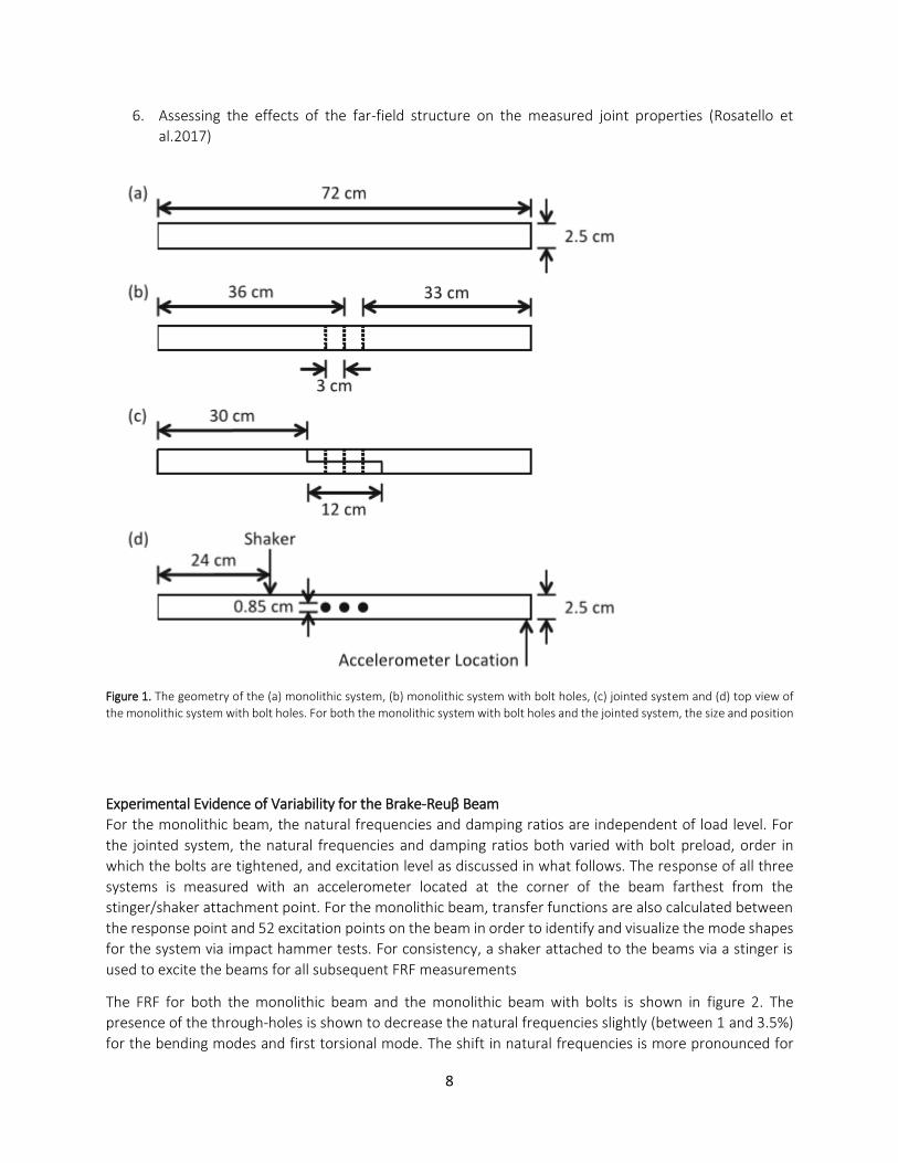
The Brake-Reuβ beam is a set of three beams, shown in figure 1. that are designed to study the influence

of a lap joint on a system’s dynamics. In all three cases, the first version of system is 72 cm long with a 2.5

cm square cross-section (more recent versions have slightly different dimensions due to being

manufactured in the USA where stock material is available in common English units instead of in Germany

where stock material is available in common metric units). For both the monolithic beam with three bolts

and the jointed beam, the bolt-holes are 0.85 cm in diameter, and located approximately along the beam’s

centerline. All of the beams are fabricated from ASTM A283 steel, with 5 cm long M8 bolts. Between the

bolt head and the beam, and between the nut and the beam on the other side of the bolt, are 0.3 cm thick

washers with a 2.1 cm outer diameter and 0.8 cm inner diameter. The first beam is a monolithic beam with

no frictional interfaces, which is used as a control to study the effect of both the bolts and lap joint. The

second beam in figure 1. is identical to the monolithic beam with the exception of three through holes. This

second beam is designed to quantify the effects of bolts themselves. The third beam in figure 1. consists of

a lap joint that is held together via three bolts.

This benchmark system has been extensively analyzed at the Nonlinear Mechanics and Dynamics (NOMAD)

Research institute, hosted by Sandia National Laboratories (Brake et al. 2015)

Current research on the Brake-Reuβ beam is focused on:

1. Characterizing the distribution of parameters to describe models representing the jointed interface

(Bonney et al.2016);

2. Developing high fidelity and reduced order models of the system (Grob et al.2016)

3. Further investigation of the application of linear methods to study this nonlinear system (Catalfamo

et al. 2016)

4. Studying how different types of stress waves propagate across the lap joint interface (Flicek et

al.2016)

5. Measuring the effects of geometric changes to the interface (Dossogne et al.2017)

8

6. Assessing the effects of the far-field structure on the measured joint properties (Rosatello et

al.2017)

Figure 1. The geometry of the (a) monolithic system, (b) monolithic system with bolt holes, (c) jointed system and (d) top view of

the monolithic system with bolt holes. For both the monolithic system with bolt holes and the jointed system, the size and position

Experimental Evidence of Variability for the Brake-Reuβ Beam

For the monolithic beam, the natural frequencies and damping ratios are independent of load level. For

the jointed system, the natural frequencies and damping ratios both varied with bolt preload, order in

which the bolts are tightened, and excitation level as discussed in what follows. The response of all three

systems is measured with an accelerometer located at the corner of the beam farthest from the

stinger/shaker attachment point. For the monolithic beam, transfer functions are also calculated between

the response point and 52 excitation points on the beam in order to identify and visualize the mode shapes

for the system via impact hammer tests. For consistency, a shaker attached to the beams via a stinger is

used to excite the beams for all subsequent FRF measurements

The FRF for both the monolithic beam and the monolithic beam with bolts is shown in figure 2. The

presence of the through-holes is shown to decrease the natural frequencies slightly (between 1 and 3.5%)

for the bending modes and first torsional mode. The shift in natural frequencies is more pronounced for

9

the second torsional mode, located near 4 kHz. This trend persists at higher frequencies as well: the bending

modes change in frequency by less than 2%, and the torsional modes differ by increasingly larger

percentages. Natural frequencies and damping ratios for all 3 beams are detailed in table 1.

Figure 2. Frequency response function (FRF) for the monolithic beam (dotted line) and the monolithic beam with bolts tightened

to 10 Nm (solid line)

Table 1. Natural frequencies for the three different beams at an excitation amplitude of 0.1 N

10

Table 2. Natural frequencies for the three different beams at an excitation amplitude of 0.1 N and 2 N

The monolithic beam with bolts does not exhibit any strong nonlinear behavior. Figure 3 presents the FRFs of the

monolithic beam with bolts at four different excitation levels (0.1, 0.5, 1, and 2 N). Aside from the small deviation near

1kHz, which could be an artifact of the shaker or stinger attachment, the response is effectively the same at all

excitation levels. By contrast, for the jointed system, the natural frequencies decrease by up to 0.3% over the same

excitation range (with the exception of the sixth bending mode, which exhibits a stiffening behavior). As detailed in

Table 2.

Figure 3. FRF for the monolithic beam with bolts at four different excitation levels and bolts preloaded to 10 Nm

The jointed system shows a high degree of variability, as is evident in figure 4, which is indicative of a strong

nonlinearity. In all experiments involving the jointed system, unless otherwise noted, the excitation amplitude is 0.1

11

N. Figure 4 presents the FRF of the system for a preload of 20 Nm on each bolt across multiple assemblies and three

different orders of the bolt being tightened. The bolts are tightened only once per assembly as preliminary

measurements indicated that there is no loss of preload during a test.

The natural frequencies and damping ratios for bending modes are relatively consistent. The torsional modes (near

3.5, 4.2, and 5.7 kHz), however, change in frequency and damping ratio each time the system is reassembled (whether

the bolts are tightened in the same order or not). This result indicates that the torsional modes are more sensitive to

the interface conditions (such as alignment, roughness, etc.), and the bending modes are more sensitive to the order

in which the bolts are tightened. The order in which the bolts are tightened is posited to be directly related to

differences in residual stresses between each assembly.

Figure 4. FRF for jointed beam with bolts tightened to a preload of 20 Nm. The different color lines correspond to different orders

in which the bolts were tightened, and the (solid) and (dashed) lines correspond to different assemblies of the system under the

same conditions

At lower preloads the bending modes (at 1.2 and 1.7 kHz in figure 5) is varied significantly in frequency and slightly in

terms of damping ratio. As the system is disassembled and reassembled using the same order of bolt tightening

(having a similar residual stress field), the natural frequencies and damping ratios of the bending modes remain

consistent, though the amplitude of the response is observed to change.

12

Figure 5. FRF for the jointed beam with bolts tightened to a preload of 5 Nm. The different color lines correspond to different

orders in which the bolts were tightened, and the (solid) and (dashed) lines correspond to different assemblies of the system under

the same conditions

As the preload of the bolts is increased to 40 Nm, shown in figure 6, the natural frequencies and damping ratios are

observed to remain approximately constant across reassembly for both the torsional mode (at 1.75 kHz) and the

bending modes. This implies that the preload is sufficiently high enough, relative to the excitation level at least, for

the system to behave linearly.

13

Figure 6. FRF for the jointed beam with bolts tightened to a preload of 40 Nm. The different color lines correspond to different

orders in which the bolts were tightened, and the (solid) and (dotted) lines correspond to different assembles of the system under

the same conditions

Resulting from the previous observation:

One class of modes (bending modes) are sensitive to the residual stresses in the system (as

correlated to the order in which the bolts are tightened)

A second class of modes (torsional modes) are so sensitive to the interfacial conditions that the

effect due to the residual stresses is not distinguishable from other effects

The Square, Four-Bolt Plate

A second benchmark system that has recently been proposed is a square, four-bolt plate. This system,

which consists of two square plates bolted together by four bolts (one located in each corner), exhibits

significantly more damping than a monolithic structure of the same dimensions. Due to its ease of

fabrication and damping characteristics, this system is a good candidate for modeling. Unlike the Brake-

Reuβ beam, which has a large, distributed contact surface, the square, four-bolt plate’s contact patches

are reduced to the area of washers located between each plate; While the configuration without washers

has been used, this introduces an additional nonlinearity due to the plates slapping. Previous iterations of

this system have determined that a six-inch plate is able to produce richer dynamics than observed in

smaller (four inch and five inch) plates. Preliminary analysis of this system is detailed in Segalman et al.2015.

The system exhibits several strong nonlinearities:

1. For multiple configurations, the amplitude dependent damping characteristics common to jointed

structures is observed.

2. When the plates are assembled without washers, an additional nonlinearity due to the plates

slapping is observed.

3. The dissipation indicates a strong dependence on the spatial location of the excitation that is

atypical of linear systems.

4. A final source of nonlinearity is hypothesized to be the two plates moving opposite one another

for several nodes (as opposed to moving in the same direction at all times). This has significant

ramifications for the modeling of the local kinematics at the bolt locations.

Thus, this system presents some rich set off nonlinearities to study for advancing the development of a

round robin system; however, the one drawback is that the joints that constitute this system are not

representative of real structure.

14

Figure 7. The geometry of the square, Four-Bolt Plate structure from top and side view

The Gaul Resonator and Dumbbell Apparatus

The Gaul Resonator (Gaul et al.1994) features a single bolt lap joint that connects two monolithic

structures, one of which is designed to have a stiffness element in it (Fig.8.a). This has the advantage of

allowing for large dynamic loads to be transmitted to the interface. Similar structures, such as the dumbbell

oscillator (Segalman et al.2009) (shown in Fig.8.b; does not include a stiffness element), are typically

designed to be massive for the natural frequencies of the structure to be relatively low, which is beneficial

for developing measurements with minimal noise and high resolution). The large dynamic loads

transmitted across the joint facilitate the study of the transition from microslip to macroslip, even with

clamping forces or preloads that are representative of industrial applications. The benefit that massive

structures have is that effects due to the attachment of sensors and excitation sources are negligible, the

15

boundary conditions are able to be better controlled, and large amounts of energy are able to be stored in

the structure for extensive ring-down testing. Further, due to the massive design and the relatively low

compliance of the joint, the structure is able to be modeled accurately with a low order discrete mass

representation featuring a nonlinear element in the location of the joint.

Figure 8. (a) Two examples of Gaul resonator, and (b) the Dumbbell apparatus

In measuring the behavior of jointed structures, it is often difficult to isolate the nonlinear behavior of one

bolted joint from other disturbing effects resulting from support structure. This system is an ideal

benchmark for measuring the transfer behavior of a bolted lap joint and also delivers the opportunity to

perform hysteresis measurements, which establishes a bridge between the two round robin challenges.

The basic design is related to the so-called dumbbell oscillator Segalman et al. (2009), consisting of two

steel masses connected by a lap joint (Fig.9)

Since the axial resonance frequencies of this arrangement lie in a quite high frequency range, the setup is

modified by a relatively soft spring, as illustratively shown in (fig.9)

16

Figure 9. Principle dumbbell oscillator and on the right side the Principle resonator setup

This operation mode of the oscillator also leads to the designation of being a “resonator” Two different

types of such resonators were developed at the University of Erlangen-Nurnberg. The first one is made of

round stock stainless steel and has a similar geometry and equal dimensions like the ones investigated in

Gaul and Bohlen (1987) and Lenz and Gaul (1995). The second one is an improved version made of flat

stock material and a different orientation of the lap joint.

The parts of the systems were manufactured from solid material and are therefore monolithic. The spring

is designed in the form of a thin bending spring (Fig.10).

Figure 10. Resonator drawings

The Cut Beam Frictional Benchmark System

The Cut Beam Frictional Benchmark System is a clamped-clamped beam excited on its first bending mode.

The beam (fig.5.3) is built up with three parts linked by two frictional interfaces. A normal pre-load is applied

to both extremities of the beam before they are clamped to the ground. Due to the pre-load, the three

parts remain in contact even during the bending motion. This design minimizes coupling between pre-load

induced normal stresses in the planar joints and the vibration-induced shear stresses due to the zero

bending moment at the location of the joints. The beam is a revision of a previous experiment (Peyret et

al.2010), and is developed with several advantageous features. The shape of the beam is designed to

maximize damping by having large interface areas, and is designed to minimize coupling between the

17

normal stresses and the vibration motion even in the case where the interfaces are located imprecisely.

Despite the form differing from that of a bolted assembly, this benchmark system reproduces the loading

conditions of an assembly under constant normal load.

Figure 11. The SUPMECA frictional benchmark system: (a) geometry and (b) isometric view

The Ampair 600 Wind Turbine (page 63)

The Ampair 600 wind turbine is one of the candidate systems and a commercially available system for the

round-robin for dissipation measurements and prediction challenge. The Ampair 600 wind turbine was the

first true benchmark system for the current generation of research challenges as it has been studied widely

and shared amongst a number of different institutions. It is not an academic system but rather a real

application. The same system is already being used as the selected test bed for Dynamics Substructuring

Focus Group.

Each substructure (e.g., the blades or the hub) is not a monolithic structure. The blades are composed of

composite materials and foam, and the central hub is potted with epoxy amongst other materials. In other

words, accurate modeling of the system requires material models that include viscous and plastic behavior.

While some methods exist to characterize this system in linearized portions of its domain, it is a more

complicated system to use as a benchmark than either the Brake-Reuβ beam or the Square, Four-Bolt Plate.

Another challenge that has become evident in analyzing the Ampair 600 Wind Turbine is that due to the

construction method, the measurement of the joint properties exhibits a higher degree of variability than

observed in other benchmark systems.

18

Figure 12. The Ampair 600 Wind Turbine test bed

The Sumali Beam

The Sumali Beam is a 20” by 2” plate with bolt holes regularly spaced along the midline with a 3” center-

to-center distance. This structure, however, exhibits very low damping ratios.

A preliminary analysis of this system is detailed in Deaner et al. (2015). This case is useful to demonstrate

the difficulty in designing a system that shows an appropriate amount of nonlinearity for both modeling

and measurements. Joints with links, such as in the Sumali Beam, tend to have significantly lower damping

than more realistic joints.

Figure 13. The geometry of the Sumali beam with one plate attached

19

Figure 14. Photo of a Sumali beam attached to a second Sumali beam

Other Benchmark Systems

The benchmark systems presented are far from an exhaustive list; however, a growing consensus amongst

researchers in this field is that they are appropriate systems to use for benchmark analyses.

From analysis of all of these systems, the essential elements of a good benchmark system are:

1. Simple and cheap to fabricate or easy to purchase.

2. Distributed contact interfaces that support large loads (in contrast to Sumali beam)

3. Easy to model materials or readily available models (in contrast to composites or foam potting).

4. Built in features that allow for a design of experiments to assess effects of the system design on

the system dynamics (such as surface roughness or structural stiffness).

5. Simpler structures that allow for smaller/faster computational models.

6. Realistic interface designs for applicability to real systems if possible.

Outlook for Adoption of Benchmark Systems

The recent research on multiple systems highlights that it is possible for meaningful analysis to be

conducted on multiple systems and for the resulting lessons to be applied to other systems. In future

research, this approach may be greatly beneficial. Additionally, if a benchmark system is selected that

provides an in-context application (such as Ampair 600 Wind Turbine), having a complimentary academic

system that is simpler to study and model would be essential.

The central question that must be asked before selecting a benchmark system then becomes: “What is the

goal of the benchmark analysis? “For projects interested in assessing variability within jointed structures, it

will be essential that the system is relatively cheap so that multiple structures can be fabricated (by

20

contrast, developing a dumbbell system with monolithic substructures may be prohibitively expensive to

study variability). If, on the other hand, the goal is to investigate the applicability of new methods to

conceptualize energy dissipation in jointed structures, then a dumbbell-like system might be the most

appropriate due to the relative ease of modeling. In either case, multiple investigations of the same system

facilitate developing a comprehensive understanding of the joint behavior, which is often unattainable by

a single lab working in isolation.

Damping

Damping due to the friction in the interface of the bolted joints dominates the overall damping in these

systems; however, the amount of damping due to friction measured in a system can differ by orders of

magnitude for experiments on two nominally identical structures. The response of the system in terms of

damping and natural frequencies is sensitive to many factors, including the interface condition (e.g.

roughness, lubrication, geometrical alignment, etc.)

Damping is a major unknown in dynamics. It controls the amplitude at which a structure vibrates and is

thus a major parameter that needs to be modeled in simulations; unfortunately, it is very poorly

understood. Furthermore, damping cannot be ignored, for example, if damping is omitted in a simulation

and resonance conditions are encountered, then the vibration amplitude is infinite, it is conjectured that

joints make a significant contribution to damping.

Damping is a general term for the various mechanisms that result in the permanent removal of energy from

a dynamic system. Thus, while most of the energy in a dynamic system is oscillating between kinetic energy

and potential energy some of the energy is lost and converted into heat or transmitted out of the system.

The loss of energy is modeled as the damping of the system.

In a structure the joints holding the structure’s components together are a source of damping. It is

suggested that the bolts and the region close to the bolts do not contribute significantly to damping.

Four sources of damping may be identifying in a built-up structure: material damping, damping due to

joints, damping within components, and damping due to transmission.

The damping sites within a bolted joint

Once this question can be answered it will enable simulations and optimizations to be performed so that

joint damping can be modeled and designed into a built-up structure.

The general idea from the studies done on a bolted joint is that, the bolts themselves and the joint are in

the proximity of the bolt do not cause any damping or at most a damping comparable with material

damping. In contrast the joint surface between bolt locations and away from the bolts (i.e., the far field)

may, if it slips, cause significant damping.

21

Considerations for Measurements of Jointed Structures The nonlinearity inherent in jointed structures is invariably affected by the boundary conditions, loading

conditions, and measurement techniques. Small changes in the experimental setup can significantly affect

the measured damping and stiffness of a joint. It is found that the hammer tests performed on the “free”

boundary condition monolithic beam has a negligible influence on the system in terms of damping ratio

and frequency variation. The time varying changes in stiffening and damping are measured by testing

multiple combinations of the experimental setup at different levels of excitation. The results showed that

the mirror-like surface finish for the interface has higher damping values compared to the rough surface

across multiple bolt torque scenarios (such as preload and tightening order) and modes of vibration.

Guidelines for a reliable measurement of features of a mechanical joint are made based on the results of

this research.

Effects of Experimental Setup To isolate the effects of mechanical joint on a system’s dynamic response is to design the test setup as

linear as possible. All test specimens are fabricated from Stainless Steel 304. The basic experimental setup

is shown in Fig.10.2, which includes the beam, two bungee cords, two PCB 356A03 Triaxial ICP

Accelerometers (Accel), two 356A02 Triaxial ICP Accelerometers used in a second experimental setup,

either a PCB 086C03 ICP Impact Hammer or a Bruel and Kjaer PM Vibration Exciter Type 4809 (shaker), LMS

16 Channel Spectral Analyzer, and a modular support rig. The excitation effects are tested in two ways: first

with the impact hammer, and second with the shaker.

Best Practices for Experiments on Jointed Systems In general, an experimental setup that is as linear as possible is recommended. Specific recommendations

from this work are:

1. For impact hammer measurements, the tip and hammer mass do not significantly affect the

measurements of damping and stiffness. Thus, the impact hammer configuration should be chosen

based on the frequency range of interest.

2. The responses of systems with free boundary conditions created via the use of bungee cords are

insensitive to the bungee length, stiffness, and position.

3. The use of accelerometers, even when they are a small fraction of the mass of the system, can

significantly affect the measurements of damping and stiffness. If used, accelerometers should be

located away from node points, and the number should be kept to a minimum.

4. For shaker excitation, care should be used in selecting an appropriate stinger. Of those tested, the

thinner stingers are found to exhibit bending, which results in the appearance of nonlinearities in

the system’s frequency responses.

5. The excitation sweep rate, magnitude, and direction are not found to have significant effects for

the present system.

6. The conditions of the interface have significant effects on the responses of the system, and future

work should aim to quantify the interface conditions thoroughly.

22

INTRODUCTION OF CONSTITUTIVE MODELS

Modeling Considerations

To develop a constitutive model of friction, there are several issues to be considered:

Physical Parameters, Lubrication, State Dependence, Model Implementation

Friction Models

1.Velocity-Based Models

1.1. Coulomb Friction This model stipulates three principles:

The area in contact has no effect on the friction force

If the load of an object is doubled, the friction force is also doubled

Friction is independent of sliding velocity

To this end, the Coulomb friction model postulates that

F = μN (1)

For a given coefficient of friction μ and normal force N. In order to implement this model numerically, it is

often convoluted with a function that either properly assigns the sign of the direction of the force:

F = μN sign (v) (2)

1.2. Viscous Friction Viscous friction is typically associated with lubrication and is seen as a term cv (with viscous coefficient c)

appended to the Coulomb friction model

𝐹 = 𝜇𝑁 + 𝑐𝑣 (3)

1.3. Stiction These models postulate that when an object is at rest, there is a higher (static) friction force needed to

initiate motion that the (dynamic) friction force once the object is moving.

𝐹 { ≤ μ𝑠N, 𝑣 = 0

= μN, 𝑣 > 0 (4)

With static coefficient μ𝑠 < μ.

23

1.4. Stribeck Friction The previous three models can be combined in multiple ways Within the Stribeck model, there are four

regimes: Static friction (v = 0), boundary lubrication (low v, F is close to the static friction force), partial

fluid lubrication (medium v ; F decreases to a local minimum), and full lubrication (high v , F strictly

increases). The Stribeck effect is based on the observation that at low velocities, friction forces decrease

with velocity, but at some point this trend is reversed and the friction forces increase with velocity once

again, as shown in Fig.14.2b

Figure 15. Illustrative examples of: (a) Coulomb friction with stiction and viscous effects, and (b) Stribeck friction

2. State-Based Models In contrast to velocity-based models, state-based models require state variable that record the state of the

model at previous time-step. In some cases, this could be condensed to a single parameter (such as Jenkin

element); in other cases, though, this can require dozens if not hundreds of variables to be tracked (such

as with the discretized Iwan model).

2.1. The LuGre Model The Lund-Grenoble (LuGre) friction model (Canudas de Wit et al. 1995; Olsson 1996), also known as the

bristle model, is the conceptualization of contact bristles (Fig.16). For simplicity, one set of bristles is

assumed to be rigid, and the other set elastic. As asperity distributions are irregular, generally, the LuGre

model is based on the average behavior of a collection of bristles that constitute the contact region.

24

Figure 16. Conceptualization of the LuGre (“Bristle”) model

2.2. The Jenkins Element The Jenkin element, attributed to Jenkins (1962), is described by an elastic friction slider, which consists of

a frictional element and spring in series as shown in Fig.17. This model is useful for describing some aspects

of microslip and macroslip behavior. The model is characterized by a tangential stiffness KT and slip force

FS = μN. Once a slip force FS is exceeded, the system transitions to pure sliding with force F = FS.

Figure 17. Jenkin Model

2.3. The Masing Element This element is used to refer to a two-dimensional Jenkins element.

25

Figure 18. Masing model

2.4. The Iwan Element Is constructed by a large number of Jenkins elements in parallel, such as shown in Fig.19. The challenge for

developing constitutive models in the Iwan element framework is describing the distribution of Jenkin

elements (in terms of stiffness and slip forces). The four-parameter Iwan model developed in Segalman

(2005) is a discretized representation of the Iwan element in which the properties of the distribution of

Jenkins element are represented with four parameters. The tangential stiffness KT, the force for inception

of macroslip FS, the exponent of the energy dissipation per cycle ꭕ, and the ratio of Jenkin elements that

slip before macroslip to those that slip at macroslip β.

Figure 19. Iwan Model

26

TEST CASE: TWO CANTILEVERED BEAMS The studying structure is made of two cantilevered beams of Aluminum as substructures which are joined

at their free-ends when assembled, as shown in Fig.25. The excitation and response points are marked as I

on beam-1 and o on beam-2 and “a” and “b” are referring to the interface points. The FRFs are obtained

experimentally using impact hammer at the points labelled as “excitation” in the figure ad the response is

measured at the points labelled as “response” on the individual beams and the assembled structure. The

response measurement is performed by Laser Doppler Vibrometers (LDV) measuring only the out-of-plane

deflections. The measured FRFs are plotted in Fig.25,26,27. The main response peaks correspond to the

bending modes. It is worth-mentioning that the four bolts (steel) for joining are considered as a part of

beam-1 and kept tightened on it during measurements acquisition.

Figure 20. The experimental configuration of the first test-case. (a) Beam-1 (b) beam-2 (both fixed-free) (c) the coupled beams (d)

the joint consisting of 4 bolts. The input and response nodes are also shown in the respective figures. The FRFs obtained on these

nodes are subsequently used for FE model updating

Additionally, the beams and the assembly are modelled in the finite element software, ANSYS APDL v17.2

with actual geometric and updated material properties as listed in table 3. The meshing is done with

SOLID186 brick element with the mid-side nodes.

Table 3. Beam properties

Properties Beam 1 Beam 2

Material Aluminium Aluminium

Dimensions 428*30*3.5 572*30*3.5

27

RESULTS

Case study Beam 1

Figure 21. Experimental FRFs of beam 1

Figure 22. Complete Beam 1 meshed with separate compressed area in the constraint end

Figure 23. Chosen nodes for the constraint of beam 1

28

Figure 24. Side view of the chosen nodes for the constraint of beam 1

Figure 25. Photo of the beam1 constraint end in the rig

Table 4. Analytical and Experimental results for beam 1 with four bolts tightened on it

Analytical results with APDL Experimental results

11.909 10.55

76.394 74.41

117.00

218.31 216.8

369.63

432.99 427.73

713.13 705.1

740.10

Average error percentage between the analytical and experimental methods for the beam with one end

constraint and the other end with four bolts mounted on it is 3.7.

29

Case Study Beam 2

Figure 26. Experimental FRFs of beam 2

Figure 27. Beam 2 meshed with the separate compressed area in the constraint end

30

Figure 28. Chosen nodes for the constraint of beam 2

Figure 29. Side view of the chosen nodes for the constraint of beam 2

Figure 30. Photo of the constraint end of the beam 2 in the rig

31

Table 5. Analytical and Experimental results for beam 2

Analytical results with APDL Experimental results 7.4264 7.41

46.660 45.9

69.952

130.96 127.92

257.28 250.4

279.50

426.56 412.7

433.86

639.47 615.6

839.68

897.17 860.5

The average error percentage between the analytical and experimental methods for the beam with one

end constraint and the other end free is 2.64.

32

Case Study of Two Cantilever Beams Assembly with four bolts

Figure 32. Complete assembly meshed

Figure 33. Meshed assembly with symbols

Figure 31. Experimental FRF of the assembly with four bolted joints

33

(a)

(b)

Figure 34. (a) Element and (b) Node plot with zoom in the contact volume part

Figure 35. Photo of the contact part with four bolts

34

Figure 36. Photo of the contact part with four bolts

Figure 37. Node numbering in the contact area of two cantilever beams

35

Figure 38. Selected nodes for merging in the contact area of two cantilever beams with four bolted joints mounted

36

Table 6. Analytical and Experimental results for the assembly with four bolts mounted it

Analytical results with APDL Experimental results 16.180 14.844

49.799 45.51

94.684 90.04

154.53 148

164.24

242.40 223.24

317.72 313.085

345.29

411.80 387

451.19 445

586.57 544.9

718.74 678.32

726.56

868.19 822.65

903.88

1031.8 1007

1099.6

1164.5 1145.3

1376.1

1420.7

At the end there is an average error of 5% between the experimental and analytical methods results.

37

IWAN MODEL INTRODUCTION

Structures with mechanical joints are not easy to model accurately; even if the natural frequencies of the

system remain constant, the damping introduced by the joint is often depending nonlinearly on amplitude.

This approach assumes that the mode shapes of the structure do not change significantly with amplitude

and there is negligible coupling between modes. The nonlinear Iwan joint model has had success in

modeling the nonlinear damping of individual joints and is used as a modal damping model. The proposed

methodology is evaluated by simulating a structure with a small number of discrete Iwan joints (bolted

joints) in a finite element code. A modal Iwan model is fit to simulated measurements from this structure

with the assessment of the modal model. The same methodology is then applied to actual experimental

hardware with a similar configuration. The proposed approach captures the response of the system in both

cases (microslip and macroslip), especially at up to moderate force levels when macroslip does not occur.

Macroslip occurs when the stick region vanishes and larger slip displacements are possible.

Figure 39. Contact and slip regions are shown for a mechanical joint undergoing microslip (Segalman 2001)

For some structure it may be possible to represent groups of joints as a single interface, or to exploit

symmetries to replicate one joint many times, but these types of approaches have not yet been thoroughly

developed. On the other hand, when a small number of modes are active in a response, some

measurements have suggested that a simpler model may be adequate. Segalman investigated the idea of

applying the four-parameter Iwan model in a modal framework in Segalman (2010), in which simulated

measurements are used to deduce the modal Iwan parameters for two simple spring mass systems and

compared to the more rigorous approach where each discrete joint in the system is treated separately.

Providing a basic introduction, an analytical case study and a review of recent experiments that support

the framework of modal modeling for structures with discrete Iwan joints; First, a finite element model of

a structure with four discrete Iwan joint is used to simulate an experiment and after that the simulated

response data is used to deduce a set of modal Iwan parameters. The approximation of the responses of

the structure with individual discrete joints with one modal Iwan model per mode are then carefully

compared to ascertain the degree to which the simpler modal model can capture the response of the higher

fidelity model. At the end, experiments on an assembly of stainless steel beams and automotive catalytic

38

converters are summarized. Both cases result that the modal Iwan model can describe the measured

response with very good accuracy.

Four-Parameter Iwan Model It is a nonlinear energy dissipation model and Mathematically, the four-parameter Iwan model is

represented as

𝐹𝐼𝑤𝑎𝑛 = ∫ ρ(φ) (u(t) − x(t, φ))dφ ∞

0 (5)

The four-parameter population density function which is a power law representation and describes a

distribution of Jenkins elements developed in Segalman (2005) has the form:

ρ(φ) = R φꭕ (H(φ) − H(φ − φmax )) + Sδ (φ − φmax ) (6)

Where, H(0) is the Heaviside step function, δ(0) is Dirac delta function, and the four parameters that

characterize joint include R, which is associated with the level of energy dissipation, ꭕ, which is directly

related to the power-law behavior of energy dissipation, φ, which is equal to the displacement at macroslip,

and the coefficient S, which accounts for a potential discontinuous slope of the force displacement plot

when macroslip occurs.

Which yields the general form of hysteresis loop shown below (Fig. 20). The parameters R and S are both

calculated from four model parameters (KT, FS, β, ꭕ).

Figure 40. Illustrative drawing of a typical hysteresis curve for a four-parameter Iwan model described by Segalman (2005)

The four parameters R, ꭕ, φ, S are converted to more physically meaningful variables KT, FS, ꭕ, β in Segalman

(2005) and Segalman and Holzmann (2005): FS is the joint force necessary to initiate macroslip, KT is the

stiffness of the joint, ꭕ is directly related to the slope of the energy dissipation in the microslip regime, and

β relates to the level of energy dissipation and the shape of the energy dissipation curve as the macroslip

force is approached. However, each joint may require a unique set of these parameters, so many joint

39

parameters need to be deduced and corresponding discrete joint models increase the cost of transient

simulations in the structural-level finite element model.

Figure 41. (a) Both macroslip force (FS) and joint stiffness (KT) can be found from the force displacement relationship of the joint.

(b) The ꭕ value is found from the slope of the dissipation and the β value is a measure of dissipation level and shape of the dissipation

curve

This new set of parameters can be deduced from the two plots Fig.41. There are a variety of methods that

could be used to find the energy dissipation and frequency by estimating them from the free response of

each mode of interest. Once these are known, the Iwan parameters can be determined using nonlinear

optimization as discussed in Segalman (2005), graphically, or through some combination of the two. This

work focuses on the graphical approach.

For a system where the damping is strictly due to the four-parameter Iwan model, the equation becomes:

M ẍ + 𝐾∞x = F𝑋 + F𝐽 (7)

With linear mass M and linear stiffness 𝐾∞ matrices of a finite element model, and vectors of external

forces F𝑋 and nonlinear joint forces F𝐽 applied to the structure which has nonzero entries corresponding

to the two ends where the joint is attached to the finite element model and depends on the history of

displacement at those points. Matrix 𝐾∞ has no contributions from the joint locations; even the linear

portion of the joint response is captured in F𝐽.

The four-parameter Iwan model has been implemented to predict the response of structures with a small

number of discrete joints (Allen and Mayes 2010; Segalman and Holzmann 2005).However, each joint may

require a unique set of parameters {Ks, Fs, ꭕ, β} so many joint parameters need to be deduced and

corresponding discrete joint models increase the cost of transient simulation in the structural-level finite

element model.

40

The Iwan Model and the Four-Parameter Iwan Model The parallel-series Iwan model (Iwan 1966, 1967) is a phenomenological model of yielding and microslip in

which the physical process is represented by the stick-slip behavior of a parallel array of Jenkins elements

with different slip threshold. Its global dynamic behavior is fully described by the frictional properties of

the Jenkins elements and the distribution ρ(φ) of Jenkins elements slipping under a displacement φ.

Adopting the dimensionless formulation of Segalman (2005), it can be shown that the force F(t) is:

F(t) = ∫ ρ(φ) (u(t) − x(t, φ)) dφ∞

0 (8)

For a displacement x(t, φ) at time t of the Jenkins element with slip displacement φ.

Assuming that these elements are massless, that the friction force is constant during slip, and that the static

and dynamic coefficients of frictions are equal (normalized).

ẋ(t, 𝜑) = {�̇�(𝑡) 𝑑𝑢𝑟𝑖𝑛𝑔 𝑠𝑙𝑖𝑝0 𝑑𝑢𝑟𝑖𝑛𝑔 𝑠𝑡𝑖𝑐𝑘

Slip onset ‖𝑢(t) −𝑥(𝑡, 𝜑)‖ = 𝜑

Under an oscillatory displacement u(t), the maximum applied force F0 is (Segalman 2005)

F0 = ∫ φ ρ(φ) dφ 𝑢0

0 + 𝑢0 ∫ ρ(φ) dφ

φ𝑚𝑎𝑥

𝑢0 (9)

Where φmax denotes the displacement at which macroslip occurs. The general dissipation of the whole

system under the harmonic motion is obtained as (Segalman 2005)

D = ∫ 4(𝑢0 – φ) φ ρ(φ) dφ𝑢0

0 (10)

Proceeding with two differentiations of Eqs. (9) and (10) with respect to 𝑢0 yields

𝜕2𝐹0

𝜕𝑢02 = −𝜌(𝑢0) (11)

and

𝜕2𝐷

𝜕𝑢02

= 4𝑢0𝜌(𝑢0)

From which it is found that

𝜕2𝐷

𝜕𝑢02 + 4𝑢0

𝜕2𝐹0

𝜕𝑢02 = 0 (13)

Subsequently it is clear that there is a relationship between F0 and D implied by the Iwan modeling

assumption which is a reflection of the dependence of both of these quantities on the single distribution

ρ(φ).

41

The four-parameter Iwan model introduced in Segalman (2005) is a specific version of the general one

above in which the distribution ρ(φ) is expressed as

ρ(φ) = R φꭕ (H(φ) − H(φ − φmax )) + Sδ (φ − φmax ) (14)

where H(0) and δ(0) are the Heaviside and Dirac delta functions. Note that the last term in the above

equation is introduced to model the occurrence of the macroslip at φ = φmax . Introducing Eq. (14) in Eqs.

(9) and (10) leads to

𝐹0 = 𝐾𝑇u0 – (Ru0

𝑥+2)

(ꭕ+1)( ꭕ+2) (15)

With tangent stiffness

𝐾𝑇 = 𝑆 + 𝑅φ𝑚𝑎𝑥

ꭕ+1

ꭕ+1 (16)

And dissipation

𝐷 =4𝑅𝑢0

ꭕ+3

(ꭕ+3) (ꭕ+2) (17)

Finally, the stiffness is defined as

𝐾 =𝐹0

𝑢0= 𝐾𝑇 −

𝑅𝑢0ꭕ+1

(ꭕ+1) (ꭕ+2) (18)

Figure 42. Extensions of the four-parameter Iwan models

42

Extended Iwan-Type Models: Five-Parameter Iwan-Type Model The four-parameter model described in the previous section is limited in its applications and does not

provide a single modeling of the force in the joint versus displacement as would be required if the joint was

part of the structure being excited. Hence, another approach to have a better representation and to reduce

epistemic uncertainty with stochastic deviations of the model and to broaden the modeling area of the

four-parameter Iwan model is necessary. Additionally, in the referring model it is allowed to have static and

dynamic coefficients of frictions, 𝜇𝑠 and 𝜇𝑑 different from each other. It is further assumed that when slip

is initiated in a Jenkins element, the force it carries drops suddenly from 𝜇𝑠𝑁 to 𝜇𝑑𝑁, and it continues to

carry until stick occurs. Therefore, we can decide the slipping Jenkin elements carry forces equal to θ times

the forces they would carry if 𝜇𝑠 = 𝜇𝑑

𝛩 = 𝜇𝑑

𝜇𝑠≤ 1

Eqs.(35.1) and (35.2) are still valid, but the slip occurrence is discontinuous

Slip onset ‖𝑢(t−) −𝑥(t−, 𝜑)‖ = 𝜑

After slip ‖𝑢(𝑡+) −𝑥(𝑡+, 𝜑)‖ = θφ

In harmonic motions, the peak value of the force F0 becomes

𝐹0 = 𝜃 ∫ 𝜑ρ(φ)𝑑𝜑𝑢0

0+ 𝑢0 ∫ 𝑅𝑂(𝜑)𝑑𝜑

𝜑𝑚𝑎𝑥

𝑢0 (19)

Instead of Eq. (9). The dissipation is obtained, as done for Eq. (10), by determining the area of the hysteresis

loop. We obtain

𝐷 = 𝜃 ∫ 4(𝑢0

0 u0 - 𝜃𝜑) 𝜑 ρ(𝜑) 𝑑𝜑 + ∫ (1 − 𝜃)2𝑢0

0𝜑2 ρ(𝜑) 𝑑𝜑 (20)

Following the arguments of Segalman et al. (2009), Segalman (2005), and Segalman and Starr (2004), it is

adopted here as in the four-parameter Iwan model, i.e., Eq. (14). Integrations yields

𝐹0 = 𝐾𝑇 𝑢0 − 𝑅[ꭕ+2−𝜃(ꭕ+1)]

(ꭕ+1)(ꭕ+2) 𝑢0

ꭕ+2 (21)

Considering the previous definition of 𝐾𝑇, i.e, Eq.(16) and

𝐷 = 𝑅[2 𝜃(ꭕ+4)+(1−3𝜃2)(ꭕ+2)]

(ꭕ+3)(ꭕ+2) 𝑢0

ꭕ+3 (22)

43

Figure 43. Hysteresis loop for the proposed five-parameter Iwan model, shown for θ=0.8

While the model proposed here involves five parameters, 𝜃 , 𝑅 , ꭕ , 𝑆 , and 𝜑𝑚𝑎𝑥

, its behavior prior to

macroslip is dictated by four parameters: 𝜃, 𝑅, ꭕ, and KT, consistently with four-parameter model, which

only involved three parameters: R, ꭕ, and 𝐾𝑇.

To give an example modeling of Sandia Joints Data with the above model of equations (21) and (22) through

the minimization of the error of is quite successful, leading to a good match of both stiffness and dissipation.

The overall focus of this part of investigations done before was the development and validation of

stochastic Iwan-type models for the characterization of a particular class of bolted joints from available

experimental data with broad scatter on its stiffness and dissipation behavior. The four-parameter parallel-

series Iwan model of Segalman (2005) was first extended to include not only differing parameters in the

modeling of the stiffness and dissipation properties but also differing static and dynamic coefficients of

friction leading to the introduction of the fifth parameter 𝜃 (the “five-parameter model”). The additional

modeling flexibility permitted the last model led to a good match of both dissipation and stiffness data.

Accordingly, this model was used to construct the desired stochastic model of the joint by randomizing only

its parameters. The statistical distribution of these parameters were selected on the basis of maximum

entropy arguments while satisfying the physical constraints of the model was identified using an

approximate maximum likelihood strategy defined on the space of the random Iwan model parameters.

Finally, the experimental data was found to fit well within the uncertainty band corresponding to the 5th

and 95th percentiles of the predictions obtained with either model which well supports their adequacy. The

methodology developed in these steps is expected to be applicable to other joint and/or joint models.

44

The Next Generation of Joints Research Stemming from the notion that the response of a jointed structure may depend upon quantities that are

outside of a designer’s control (such as grain distribution), these quantities should be accounted for using

uncertainty characterization techniques for epistemic uncertainty. Other parameters, particularly as

related to geometry and material properties, should serve as direct inputs to an ideal joint model. Related

to this, the conceptualization of parameters as being deterministic is limiting our approach to modeling

jointed structures. It must be recognized that all parameters within a model are stochastic by nature, and

the techniques for measuring and incorporating them into a model must reflect this.

On Numerical Modeling With the advance of Iwan and other hysteretic friction models, there now exist multiple high fidelity

constitutive representations of the hysteresis observed in frictional evets. However, at the same time, it

has become apparent that an accurate (calibrated) constitutive model of a hysteretic process is not enough

for developing an accurate numerical model of a jointed structure. Due to the coupling of structures and

modes inherent to nonlinearities and to the local kinematics, careful attention to the spatial modeling and

coupling is needed. It is not enough to calibrate a friction model without considering the effects of the local

kinematics within a joint. Instead, as new insights are gained into how to couple two different substructures

at a jointed interface, the ideal constitutive model may, in isolation, not resemble the system’s response,

which is a product of contact across an entire flexible interface, not just a point. Thus, a reasonable

hypothesis is The spatial modeling of interactions within a jointed interface is as important, if not more so,

than the constitutive modeling of the hysteresis exhibited by the system.