Presented at “Short Course V on Conceptual Modelling of Geothermal Systems”, organized by UNU-GTP and LaGeo, in Santa Tecla, El Salvador, February 24 - March 2, 2013.

1

LaGeo S.A. de C.V. GEOTHERMAL TRAINING PROGRAMME

DYNAMIC MODELLING OF GEOTHERMAL SYSTEMS

Gudni Axelsson Iceland GeoSurvey (ÍSOR)

Grensásvegur 9, IS-108 Reyjavík and University of Iceland

Saemundargata 1, IS-101 Reykjavík ICELAND gax@isor.is

ABSTRACT The energy production capacity of hydrothermal systems is predominantly con-trolled by the reservoir pressure decline caused by the hot water production, which is in turn determined by the size of a geothermal reservoir, its permeability, reservoir storage capacity, water recharge and geological structure. More generally the capacity of all geothermal systems is also controlled by their energy content, dictated by their size and temperature conditions (enthalpy if two-phase). Hydrothermal systems can in most cases be classified as either closed, with limited or no recharge, or open, where recharge equilibrates with the mass extraction in the long run. Modelling plays a key role in understanding the nature of geothermal systems and is the most powerful tool for predicting their response to future production. Predictions are used to estimate their production capacity. Reliable models are also an indispensable part of successful geothermal resource management during utilization. In addition to the volumetric assessment method (static modelling) different methods of dynamic modelling are the main techniques used for geothermal reservoir modelling and resource assessment. The dynamic modelling methods apply simple analytical models, lumped parameter models or detailed numerical models to simulate the nature and production response of geothermal systems as well as to calculate future predictions. The modelling method applied should be determined by the purpose of a study and the data available for calibrating a model, as the time and cost involved are highly variable. All reliable models of geothermal systems, whether static or dynamic, should be based on an accurate conceptual model of the corresponding system. The results of geothermal system modelling may, moreover, lead to changes in their respective conceptual models.

1. INTRODUCTION Geothermal resources are distributed throughout the Earth’s crust with the greatest energy concentration associated with hydrothermal systems in volcanic regions at crustal plate boundaries. Yet exploitable geothermal resources may be found in most countries, either as warm ground-water in sedimentary formations or in deep circulation systems in crystalline rocks. Shallow thermal energy suitable for ground-source heat-pump utilization is available world-wide and attempts are underway at developing enhanced geothermal systems (EGS) in places where limited permeability precludes natural hydrothermal activity. Saemundsson et al. (2009) discuss the classification and geological setting of geothermal systems in considerable detail.

Axelsson 2 Dynamic modelling

The potential of the Earth’s geothermal resources is enormous when compared to its use today and to the future energy needs of mankind. Stefánsson (2005) estimated the technically feasible electrical generation potential of identified geothermal resources to be 240 GWe (1 GW = 109 W), which are likely to be only a small fraction of unidentified resources. He also indicated the most likely direct use potential of lower temperature resources (< 150°C) to be 140 EJ/yr (1 EJ = 1018 J). The Earth’s ultimate geothermal potential is, however, impossible to estimate accurately at the present stage of knowledge and technology. Even though geothermal energy utilization has been growing rapidly in recent years, it is still miniscule compared with the Earth’s potential. Bertani (2010) estimated the worldwide installed geothermal electricity generation capacity to have been about 10.7 GWe in 2010 and Lund et al. (2010) estimated the direct geothermal utilization in 2009 to have amounted to 438 PJ/yr (1 PJ = 1015 J). The successful exploration, development and utilization of a geothermal resource rely on efficient collaboration between various scientific disciplines as well as engineering during all stages. During the exploration stage of a geothermal resource research focuses on analysis of surface exploration data; mainly geological, geophysical and geochemical data, while this emphasis shifts to reservoir physics research during development and utilization. Geothermal reservoir physics, commonly also called geothermal reservoir engineering, is the scientific discipline that deals with mass and energy transfer in geothermal systems and geothermal wells. It attempts to understand and quantify this flow along with accompanying changes in reservoir conditions, in particular those caused by exploitation. The purpose of geothermal reservoir physics is, in fact, twofold; to obtain information on the nature, reservoir properties and physical conditions in a geothermal system and to use this information to predict the response of reservoirs and wells to exploitation. Based on the latter the energy production capacity of a geothermal resource can be assessed, which actually can be termed the fundamental issue of geothermal reservoir physics. Geothermal reservoir physics is e.g. discussed in more detail by Bödvarsson and Witherspoon (1989), Grant and Bixley (2011) and Axelsson (2012). Diverse types of model calculations are the principal tools of geothermal reservoir physics, and as such play a key role in overall geothermal research. Modelling is used to analyse various types of reservoir engineering data, such as pressure transient data (Axelsson, 2013), with the purpose of providing estimates of different reservoir properties (e.g. permeability). Once reservoir properties and physical conditions have been estimated, subsequent models are used to simulate the conditions and changes in the geothermal system in question, both during the pre-exploitation stage (natural state) and during utilization (production state). Modelling thus plays a key role in understanding the nature of geothermal systems as well as being the most powerful tool for predicting their response to future production. Reliable models are also an indispensable part of successful geothermal resource management during utilization, since response predictions can e.g. aid in foreseeing the outcome different management actions (Axelsson, 2008b). The modelling methods used in geothermal development can be classified as either static or dynamic methods. The volumetric assessment method, discussed by Sarmiento et al. (2013) at this Short Course, is the principal static modelling method. It is used to estimate the static energy content of a geothermal system and its possible utilization (extraction). Yet the different methods of dynamic modelling are the main techniques used for geothermal reservoir modelling and resource assessment. The dynamic modelling methods apply simple analytical models, lumped parameter models or detailed numerical models to simulate the nature and production response of geothermal systems as well as to calculate future predictions. Modelling of geothermal systems, in particular detailed numerical modelling, is e.g. discussed by Bödvarsson et al. (1986), O’Sullivan et al. (2001) and Pruess (2002). Models of geothermal systems are calibrated by various reservoir physics data, e.g. well test and monitoring data. In addition they should be based on other relevant geo-scientific data, generally more indirectly. All reliable models of geothermal systems, whether static or dynamic, should thus be based on an accurate conceptual model of the corresponding system, which is the subject of this Short Course. The results of geothermal system modelling may, moreover, provide input into the development, or

Dynamic modelling 3 Axelsson

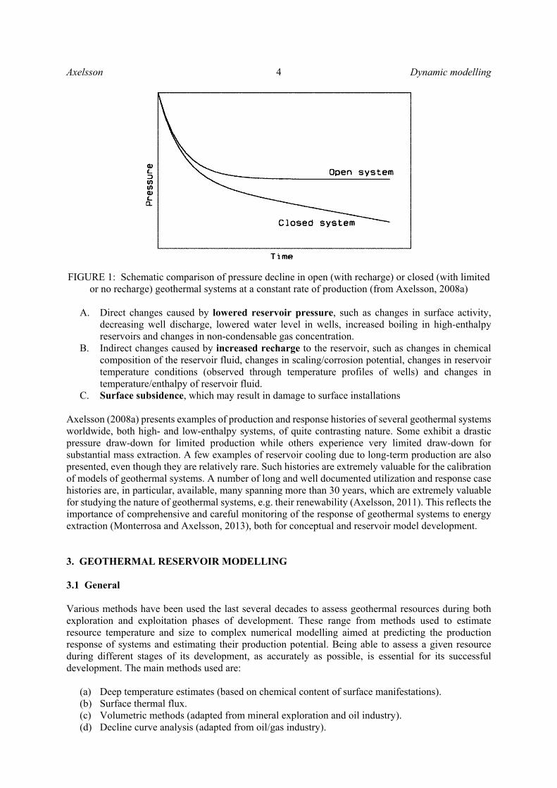
revision, of conceptual models geothermal systems, or lead to changes therein, e.g. if the modelling indicates discrepancies between what appears to be physically acceptable and the conceptual model. This paper starts out by discussing the factors which control the nature and energy production capacity of geothermal systems. The main emphasis is, however, on reviewing the different methods of dynamic modelling of geothermal systems, including their strengths and weaknesses along with data requirements. The paper is concluded by general conclusions and recommendations. 2. NATURE AND PRODUCTION CAPACITY OF GEOTHERMAL SYSTEMS The long-term response and hence production capacity of geothermal systems is mainly controlled by (1) their size and energy content, (2) permeability structure, (3) boundary conditions (i.e. significance of natural and production induced recharge) and (4) reinjection management. Their energy production potential, in particular in the case of hydrothermal systems, is predominantly determined by pressure decline due to production. This is because there are technical limits to how great a pressure decline in a well is allowable; because of pump depth or spontaneous discharge through boiling, for example. The production potential is also determined by the available energy content of the system, i.e. by its size and the temperature or enthalpy of the extracted mass. The pressure decline is determined by the rate of production, on one hand, and the nature and characteristics of the geothermal system, on the other hand. Natural geothermal reservoirs can often be classified as either open or closed, with drastically different long-term behaviour, depending on their boundary conditions (see also Figure1):

(A) Pressure declines continuously with time, at constant production, in systems that are closed or with small recharge (relative to the production). In such systems the production potential is limited by lack of water rather than lack of thermal energy. Such systems are ideal for reinjection, which provides man-made recharge. Examples are many sedimentary geothermal systems, systems in areas with limited tectonic activity or systems sealed off from surrounding hydrological systems by chemical precipitation.

(B) Pressure stabilizes in open systems because recharge eventually equilibrates with the mass extraction. The recharge may be both hot deep recharge and colder shallow recharge. The latter will eventually cause reservoir temperature to decline and production wells to cool down. In such systems the production potential is limited by the reservoir energy content (temperature and size) as the energy stored in the reservoir rocks will heat up the colder recharge as long as it is available/accessible.

The situation is somewhat different for EGS-systems and sedimentary systems utilized through production-reinjection doublets (well-pairs) and heat-exchangers with 100% reinjection. Then the production potential is predominantly controlled by the energy content of the systems involved. But permeability, and therefore pressure variations, is also of controlling significance in such situations. This is because it controls the pressure response of the wells and how much flow can be achieved and maintained, for example through the doublets involved (it’s customary to talk about intra-well impedance for EGS-systems, based on the electrical analogy). In sedimentary systems the permeability is natural but in EGS-systems the permeability is to a large degree man-made, or at least enhanced. Water or steam extraction from a geothermal reservoir causes, in all cases, some decline in reservoir pressure, as already discussed. The only exception is when production from a reservoir is less than its natural recharge and discharge. Consequently, the pressure decline manifests itself in further changes, which for natural geothermal systems may be summarised in a somewhat simplified manner as follows:

Axelsson 4 Dynamic modelling

FIGURE 1: Schematic comparison of pressure decline in open (with recharge) or closed (with limited or no recharge) geothermal systems at a constant rate of production (from Axelsson, 2008a)

A. Direct changes caused by lowered reservoir pressure, such as changes in surface activity,

decreasing well discharge, lowered water level in wells, increased boiling in high-enthalpy reservoirs and changes in non-condensable gas concentration.

B. Indirect changes caused by increased recharge to the reservoir, such as changes in chemical composition of the reservoir fluid, changes in scaling/corrosion potential, changes in reservoir temperature conditions (observed through temperature profiles of wells) and changes in temperature/enthalpy of reservoir fluid.

C. Surface subsidence, which may result in damage to surface installations Axelsson (2008a) presents examples of production and response histories of several geothermal systems worldwide, both high- and low-enthalpy systems, of quite contrasting nature. Some exhibit a drastic pressure draw-down for limited production while others experience very limited draw-down for substantial mass extraction. A few examples of reservoir cooling due to long-term production are also presented, even though they are relatively rare. Such histories are extremely valuable for the calibration of models of geothermal systems. A number of long and well documented utilization and response case histories are, in particular, available, many spanning more than 30 years, which are extremely valuable for studying the nature of geothermal systems, e.g. their renewability (Axelsson, 2011). This reflects the importance of comprehensive and careful monitoring of the response of geothermal systems to energy extraction (Monterrosa and Axelsson, 2013), both for conceptual and reservoir model development. 3. GEOTHERMAL RESERVOIR MODELLING 3.1 General Various methods have been used the last several decades to assess geothermal resources during both exploration and exploitation phases of development. These range from methods used to estimate resource temperature and size to complex numerical modelling aimed at predicting the production response of systems and estimating their production potential. Being able to assess a given resource during different stages of its development, as accurately as possible, is essential for its successful development. The main methods used are:

(a) Deep temperature estimates (based on chemical content of surface manifestations). (b) Surface thermal flux. (c) Volumetric methods (adapted from mineral exploration and oil industry). (d) Decline curve analysis (adapted from oil/gas industry).

Dynamic modelling 5 Axelsson

(e) Simple mathematical modelling (often analytical). (f) Lumped parameter modelling. (g) Detailed numerical modelling of natural state and/or exploitation state (often called distributed

parameter models). The first two methods are not modelling methods per se, but are the methods that can be used for resource assessment prior to extensive geophysical surveying and drilling. The remaining methods in the list can all be considered modelling methods, which play an essential role in geothermal resource development and management. These range from basic volumetric resource assessment (c) and simple analytical modelling (e) of the results of a short well test to detailed numerical modelling (g) of a complex geothermal system, simulating an intricate pattern of changes resulting from long-term production. In the early days of geothermal reservoir studies decline curve analysis (d) proved to be an efficient method to predict the future output of individual high-temperature wells (Bödvarsson and Witherspoon, 1989), but today other modelling methods are usually applied. Decline curve analysis is particularly applicable to wells in dry-steam reservoirs. The purpose of geothermal modelling is firstly to obtain information on the conditions in a geothermal system as well as on the nature and properties of the system. This leads to proper understanding of its nature and successful development of the resource. Secondly, the purpose of modelling is to predict the response of the reservoir to future production and estimate the production potential of the system as well as to estimate the outcome of different management actions. The diverse information, which is the foundation for all reservoir-modelling, needs to be continuously gathered throughout the exploration and exploitation history of a geothermal reservoir. Information on reservoir properties is obtained by disturbing the state of the reservoir (fluid-flow, pressure) and by observing the resulting response, and is done through well and reservoir testing and data collection (Axelsson, 2013). Different methods of testing geothermal reservoirs are available (Axelsson and Steingrímsson, 2012), but it should be emphasised that the data collected does not give the reservoir properties directly. Instead, the data are interpreted, or analysed, on the basis of appropriate models yielding estimates of reservoir properties. It is important to keep in mind that the resulting values are model-dependent, i.e. different models give different estimates. It is also very important to keep in mind that the longer, and more extensive the tests are, the more information is obtained on the system in question. Therefore, the most important data on a geothermal reservoir is obtained through careful monitoring during long-term exploitation (Monterrosa and Axelsson, 2013), which can be looked upon as prolonged and extensive reservoir testing. The modelling methods may be classified as either static modelling methods or dynamic modelling methods, with the volumetric method (c) being the main static method. Both involve development of some kind of a mathematical model that simulates some, or most, of the data available on the system involved. The volumetric method is based on estimating the total heat stored in a volume of rock and how much of that can be efficiently recovered (Sarmiento et al., 2013). The dynamic modelling methods ((d) – (g) in the list above) are based on modelling the dynamic conditions and behaviour (production response) of geothermal systems. These are the main subject of the present paper. The volumetric method, which is discussed in a separate presentation at the present short course (Sarmiento et al., 2013) is the main static modelling method, as already stated. It is often used for first stage assessment, when data are limited, and was more commonly used in the past (Muffler and Cataldi, 1978; Rybach and Muffler, 1981), but is still the main assessment method in some countries. It is increasingly being used, however, through application of the Monte Carlo method (Sarmiento et al., 2013; see also Sarmiento and Björnsson, 2007). This method enables the incorporation of overall uncertainty in the results. The main drawback of the volumetric method is the fact that the dynamic response of a reservoir to production is not considered, such as the pressure response and the effect of fluid recharge. Reservoirs with the same heat content may have different permeabilities and recharge and, hence, very different production potentials.

Axelsson 6 Dynamic modelling

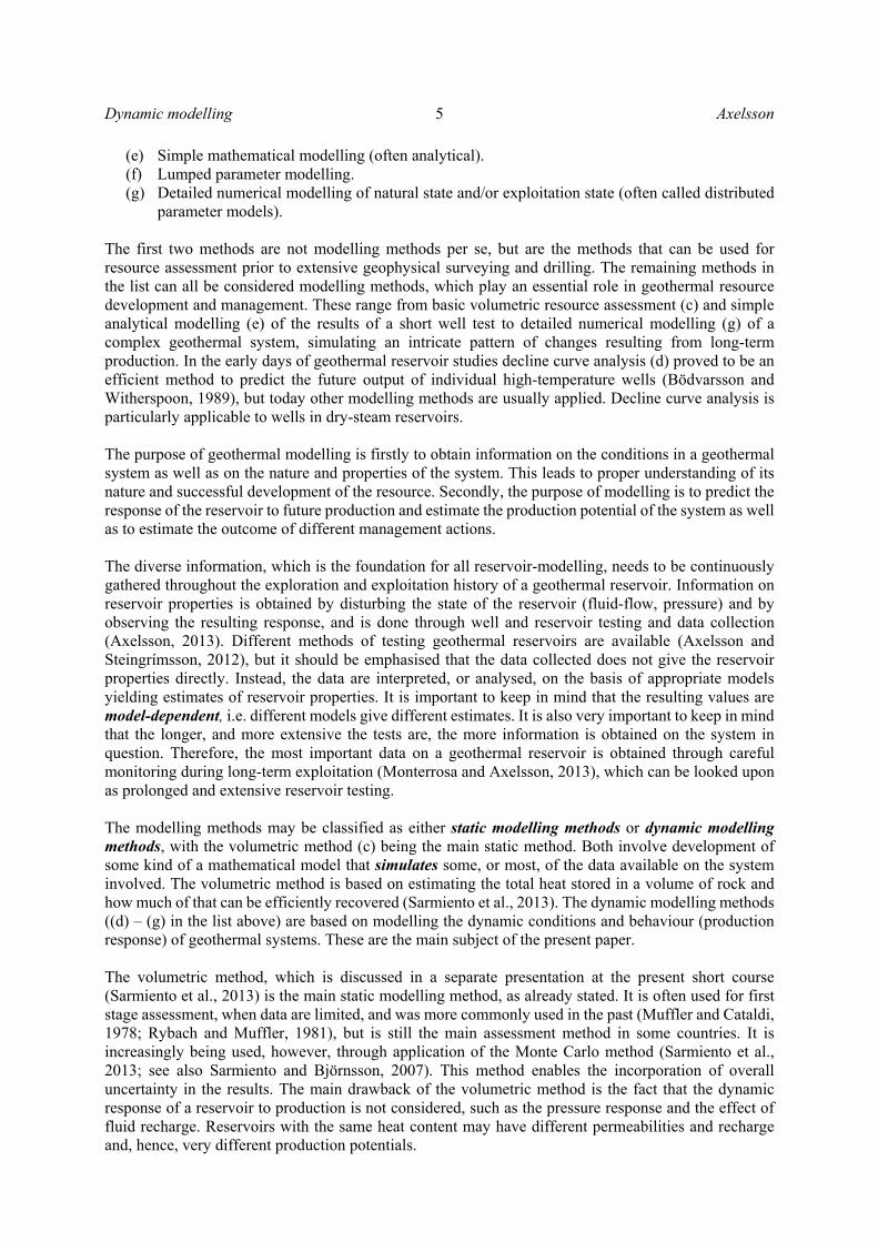
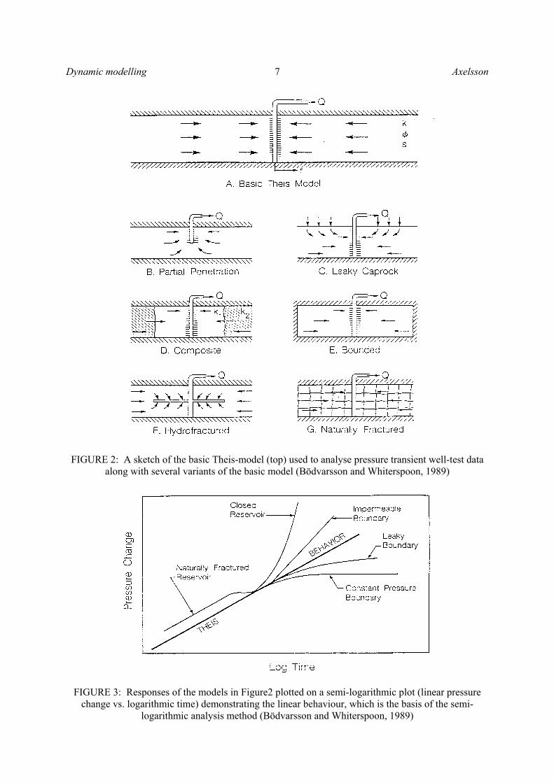
The main dynamic modelling methods applied to geothermal systems are simple mathematical (analytical) modelling methods (e), lumped parameter methods (f) and detailed numerical modelling (g), as listed above. The initial phase of such model development should be based on a good conceptual model of the geothermal system in question (Bödvarsson et al., 1986; Pruess, 2002), which is a qualitative or descriptive model incorporating all the essential features of a geothermal system revealed by analysis of all available data, as described in detail at the present short course. The next step is the development of a quantitative natural state model, which should simulate the physical state of a geothermal system prior to production. Finally, an exploitation model is developed to simulate changes in the physical state of a system during long-term production, and to calculate predictions as well as for other management purposes. Numerous examples are available on the successful role of modelling in geothermal resource management (Axelsson and Gunnlaugsson, 2000; O’Sullivan et al., 2001). In simple models, such as simple analytical models and lumped parameter models, the real structure and spatially variable properties of a geothermal system are greatly simplified so that analytical mathematical equations, describing the response of the model to energy production may be derived. These models, in fact, often only simulate one aspect of a geothermal system’s response. In such models the natural state is, furthermore, simply given by the initial conditions assumed. Detailed and complex numerical models, on the other hand, can accurately simulate most aspects of a geothermal system’s structure, conditions and response to production. Simple modelling takes relatively little time and only requires limited data on a geothermal system and its response, whereas numerical modelling takes a long time and requires powerful computers as well as comprehensive and detailed data on the system in question. The complexity of a model should be determined by the purpose of a study, the data available and its relative cost. In fact, simple modelling, such as lumped parameter modelling, is often a cost-effective and timesaving alternative. It may be applied in situations when available data are limited, when funds are restricted, or as parts of more comprehensive studies, such as to validate results of numerical modelling studies. 3.2 Simple modelling Simple mathematical models wherein the real structure and spatially variable properties of geothermal systems are greatly simplified, so that analytical mathematical equations describing their response may be derived, have been used extensively in geothermal reservoir engineering. Many examples are e.g. given by Grant and Bixeley (2011). Many of these simple models have been inherited from ground-water science or even adopted from theoretical heat conduction treatises (because the pressure diffusion and heat conduction equations have exactly the same mathematical form). A good example of the former is the well-known Theis model, a sketch of which is presented in Figure 4, along with sketches of a few variants of the basic model. The Theis model comprises a model of a very extensive horizontal, permeable layer of constant thickness, confined at the top and bottom, with two-dimensional, horizontal flow towards a producing well extending through the layer. Geothermal well-test data are often analysed on basis of the Theis model, and its variants, by fitting the pressure response of the model(s) to observed pressure response data. Consequently the parameters of the model provide an estimate of the parameters of the reservoir being tested. Figure 5 shows the calculated responses of the Theis model and its variants (Figure 2), on a semi-logarithmic plot. Simple modelling has been used extensively to study and manage the low-temperature geothermal systems utilised in Iceland, in particular to model their long-term response to production (Axelsson and Gunnlaugsson, 2000). Lumped parameter modelling of water level and pressure change data, has been the principal tool for this purpose (Axelsson et al., 2005). Lumped models can simulate such data very accurately, even very long data sets (several decades). Lumped parameter modelling will be discussed in more detail below. It plainly illustrates the general methodology of geothermal modelling.

Dynamic modelling 7 Axelsson

FIGURE 2: A sketch of the basic Theis-model (top) used to analyse pressure transient well-test data along with several variants of the basic model (Bödvarsson and Whiterspoon, 1989)

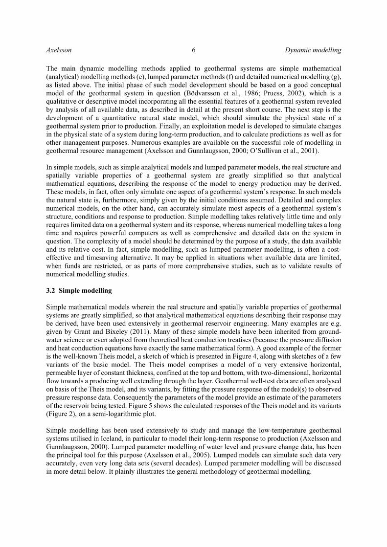
FIGURE 3: Responses of the models in Figure2 plotted on a semi-logarithmic plot (linear pressure change vs. logarithmic time) demonstrating the linear behaviour, which is the basis of the semi-

logarithmic analysis method (Bödvarsson and Whiterspoon, 1989)

Axelsson 8 Dynamic modelling

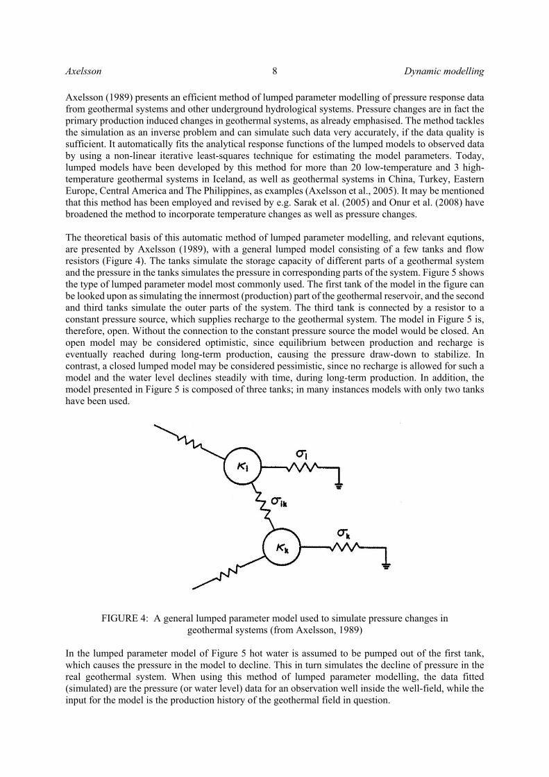
Axelsson (1989) presents an efficient method of lumped parameter modelling of pressure response data from geothermal systems and other underground hydrological systems. Pressure changes are in fact the primary production induced changes in geothermal systems, as already emphasised. The method tackles the simulation as an inverse problem and can simulate such data very accurately, if the data quality is sufficient. It automatically fits the analytical response functions of the lumped models to observed data by using a non-linear iterative least-squares technique for estimating the model parameters. Today, lumped models have been developed by this method for more than 20 low-temperature and 3 high-temperature geothermal systems in Iceland, as well as geothermal systems in China, Turkey, Eastern Europe, Central America and The Philippines, as examples (Axelsson et al., 2005). It may be mentioned that this method has been employed and revised by e.g. Sarak et al. (2005) and Onur et al. (2008) have broadened the method to incorporate temperature changes as well as pressure changes. The theoretical basis of this automatic method of lumped parameter modelling, and relevant equtions, are presented by Axelsson (1989), with a general lumped model consisting of a few tanks and flow resistors (Figure 4). The tanks simulate the storage capacity of different parts of a geothermal system and the pressure in the tanks simulates the pressure in corresponding parts of the system. Figure 5 shows the type of lumped parameter model most commonly used. The first tank of the model in the figure can be looked upon as simulating the innermost (production) part of the geothermal reservoir, and the second and third tanks simulate the outer parts of the system. The third tank is connected by a resistor to a constant pressure source, which supplies recharge to the geothermal system. The model in Figure 5 is, therefore, open. Without the connection to the constant pressure source the model would be closed. An open model may be considered optimistic, since equilibrium between production and recharge is eventually reached during long-term production, causing the pressure draw-down to stabilize. In contrast, a closed lumped model may be considered pessimistic, since no recharge is allowed for such a model and the water level declines steadily with time, during long-term production. In addition, the model presented in Figure 5 is composed of three tanks; in many instances models with only two tanks have been used.

FIGURE 4: A general lumped parameter model used to simulate pressure changes in geothermal systems (from Axelsson, 1989)

In the lumped parameter model of Figure 5 hot water is assumed to be pumped out of the first tank, which causes the pressure in the model to decline. This in turn simulates the decline of pressure in the real geothermal system. When using this method of lumped parameter modelling, the data fitted (simulated) are the pressure (or water level) data for an observation well inside the well-field, while the input for the model is the production history of the geothermal field in question.

Dynamic modelling 9 Axelsson

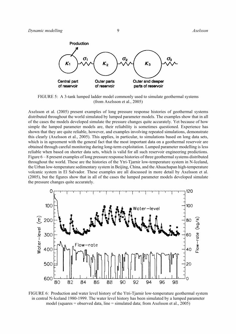
FIGURE 5: A 3-tank lumped ladder model commonly used to simulate geothermal systems (from Axelsson et al., 2005)

Axelsson et al. (2005) present examples of long pressure response histories of geothermal systems distributed throughout the world simulated by lumped parameter models. The examples show that in all of the cases the models developed simulate the pressure changes quite accurately. Yet because of how simple the lumped parameter models are, their reliability is sometimes questioned. Experience has shown that they are quite reliable, however, and examples involving repeated simulations, demonstrate this clearly (Axelsson et al., 2005). This applies, in particular, to simulations based on long data sets, which is in agreement with the general fact that the most important data on a geothermal reservoir are obtained through careful monitoring during long-term exploitation. Lumped parameter modelling is less reliable when based on shorter data sets, which is valid for all such reservoir engineering predictions. Figure 6 – 8 present examples of long pressure response histories of three geothermal systems distributed throughout the world. These are the histories of the Ytri-Tjarnir low-temperature system in N-Iceland, the Urban low-temperature sedimentary system in Beijing, China, and the Ahuachapan high-temperature volcanic system in El Salvador. These examples are all discussed in more detail by Axelsson et al. (2005), but the figures show that in all of the cases the lumped parameter models developed simulate the pressure changes quite accurately.

FIGURE 6: Production and water level history of the Ytri-Tjarnir low-temperature geothermal system in central N-Iceland 1980-1999. The water level history has been simulated by a lumped parameter

model (squares = observed data, line = simulated data; from Axelsson et al., 2005)

Axelsson 10 Dynamic modelling

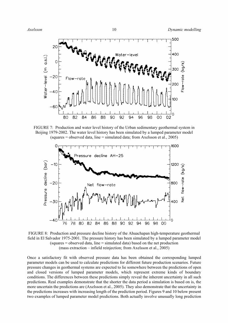
FIGURE 7: Production and water level history of the Urban sedimentary geothermal system in Beijing 1979-2002. The water level history has been simulated by a lumped parameter model

(squares = observed data, line = simulated data; from Axelsson et al., 2005)

FIGURE 8: Production and pressure decline history of the Ahuachapan high-temperature geothermal field in El Salvador 1975-2001. The pressure history has been simulated by a lumped parameter model

(squares = observed data, line = simulated data) based on the net production (mass extraction – infield reinjection; from Axelsson et al., 2005)

Once a satisfactory fit with observed pressure data has been obtained the corresponding lumped parameter models can be used to calculate predictions for different future production scenarios. Future pressure changes in geothermal systems are expected to lie somewhere between the predictions of open and closed versions of lumped parameter models, which represent extreme kinds of boundary conditions. The differences between these predictions simply reveal the inherent uncertainty in all such predictions. Real examples demonstrate that the shorter the data period a simulation is based on is, the more uncertain the predictions are (Axelsson et al., 2005). They also demonstrate that the uncertainty in the predictions increases with increasing length of the prediction period. Figures 9 and 10 below present two examples of lumped parameter model predictions. Both actually involve unusually long prediction

Dynamic modelling 11 Axelsson

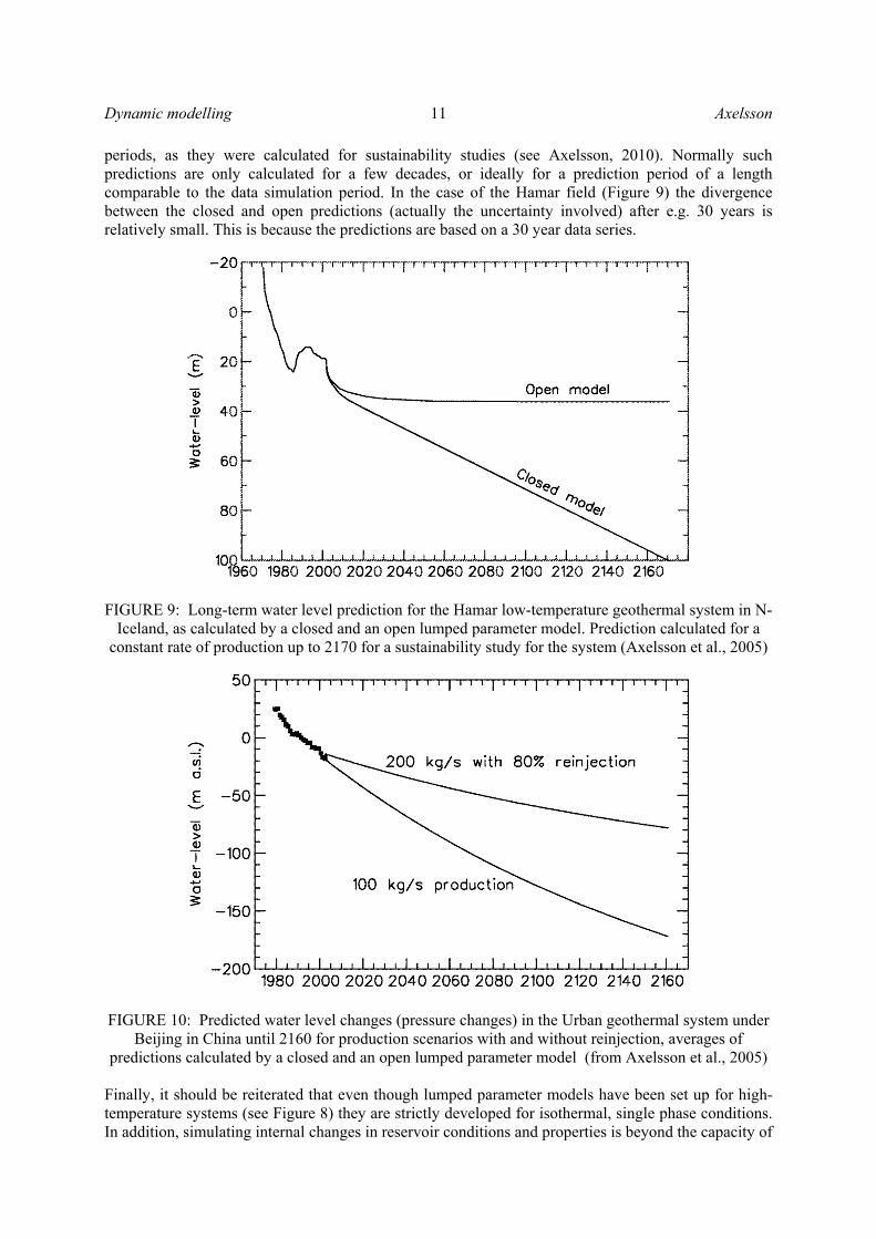
periods, as they were calculated for sustainability studies (see Axelsson, 2010). Normally such predictions are only calculated for a few decades, or ideally for a prediction period of a length comparable to the data simulation period. In the case of the Hamar field (Figure 9) the divergence between the closed and open predictions (actually the uncertainty involved) after e.g. 30 years is relatively small. This is because the predictions are based on a 30 year data series.

FIGURE 9: Long-term water level prediction for the Hamar low-temperature geothermal system in N-Iceland, as calculated by a closed and an open lumped parameter model. Prediction calculated for a

constant rate of production up to 2170 for a sustainability study for the system (Axelsson et al., 2005)

FIGURE 10: Predicted water level changes (pressure changes) in the Urban geothermal system under Beijing in China until 2160 for production scenarios with and without reinjection, averages of

predictions calculated by a closed and an open lumped parameter model (from Axelsson et al., 2005) Finally, it should be reiterated that even though lumped parameter models have been set up for high-temperature systems (see Figure 8) they are strictly developed for isothermal, single phase conditions. In addition, simulating internal changes in reservoir conditions and properties is beyond the capacity of

Axelsson 12 Dynamic modelling

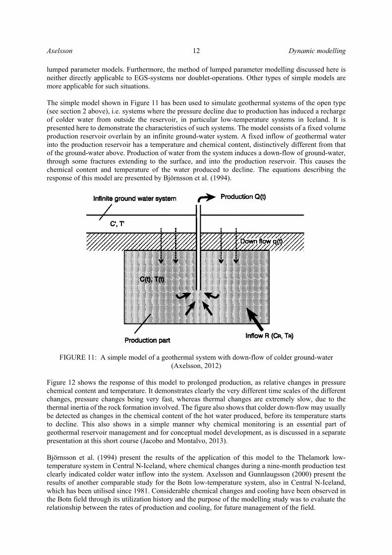
lumped parameter models. Furthermore, the method of lumped parameter modelling discussed here is neither directly applicable to EGS-systems nor doublet-operations. Other types of simple models are more applicable for such situations. The simple model shown in Figure 11 has been used to simulate geothermal systems of the open type (see section 2 above), i.e. systems where the pressure decline due to production has induced a recharge of colder water from outside the reservoir, in particular low-temperature systems in Iceland. It is presented here to demonstrate the characteristics of such systems. The model consists of a fixed volume production reservoir overlain by an infinite ground-water system. A fixed inflow of geothermal water into the production reservoir has a temperature and chemical content, distinctively different from that of the ground-water above. Production of water from the system induces a down-flow of ground-water, through some fractures extending to the surface, and into the production reservoir. This causes the chemical content and temperature of the water produced to decline. The equations describing the response of this model are presented by Björnsson et al. (1994).

FIGURE 11: A simple model of a geothermal system with down-flow of colder ground-water (Axelsson, 2012)

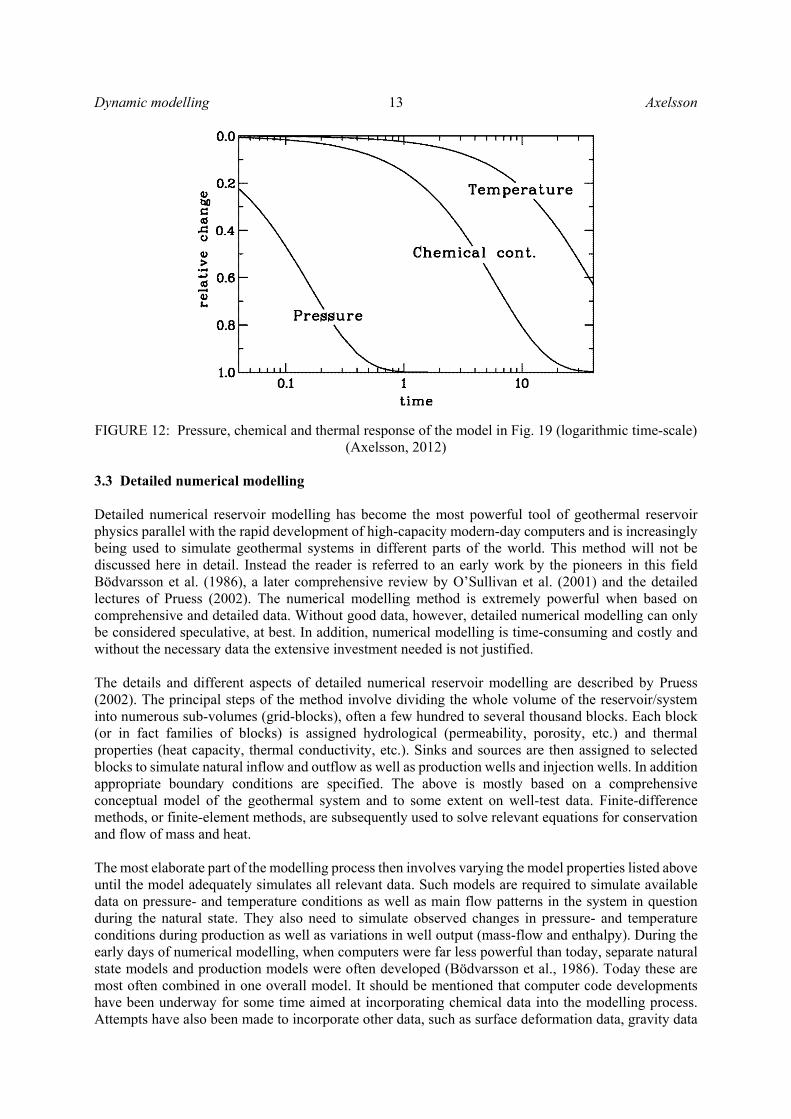
Figure 12 shows the response of this model to prolonged production, as relative changes in pressure chemical content and temperature. It demonstrates clearly the very different time scales of the different changes, pressure changes being very fast, whereas thermal changes are extremely slow, due to the thermal inertia of the rock formation involved. The figure also shows that colder down-flow may usually be detected as changes in the chemical content of the hot water produced, before its temperature starts to decline. This also shows in a simple manner why chemical monitoring is an essential part of geothermal reservoir management and for conceptual model development, as is discussed in a separate presentation at this short course (Jacobo and Montalvo, 2013). Björnsson et al. (1994) present the results of the application of this model to the Thelamork low-temperature system in Central N-Iceland, where chemical changes during a nine-month production test clearly indicated colder water inflow into the system. Axelsson and Gunnlaugsson (2000) present the results of another comparable study for the Botn low-temperature system, also in Central N-Iceland, which has been utilised since 1981. Considerable chemical changes and cooling have been observed in the Botn field through its utilization history and the purpose of the modelling study was to evaluate the relationship between the rates of production and cooling, for future management of the field.

Dynamic modelling 13 Axelsson

FIGURE 12: Pressure, chemical and thermal response of the model in Fig. 19 (logarithmic time-scale) (Axelsson, 2012)

3.3 Detailed numerical modelling Detailed numerical reservoir modelling has become the most powerful tool of geothermal reservoir physics parallel with the rapid development of high-capacity modern-day computers and is increasingly being used to simulate geothermal systems in different parts of the world. This method will not be discussed here in detail. Instead the reader is referred to an early work by the pioneers in this field Bödvarsson et al. (1986), a later comprehensive review by O’Sullivan et al. (2001) and the detailed lectures of Pruess (2002). The numerical modelling method is extremely powerful when based on comprehensive and detailed data. Without good data, however, detailed numerical modelling can only be considered speculative, at best. In addition, numerical modelling is time-consuming and costly and without the necessary data the extensive investment needed is not justified. The details and different aspects of detailed numerical reservoir modelling are described by Pruess (2002). The principal steps of the method involve dividing the whole volume of the reservoir/system into numerous sub-volumes (grid-blocks), often a few hundred to several thousand blocks. Each block (or in fact families of blocks) is assigned hydrological (permeability, porosity, etc.) and thermal properties (heat capacity, thermal conductivity, etc.). Sinks and sources are then assigned to selected blocks to simulate natural inflow and outflow as well as production wells and injection wells. In addition appropriate boundary conditions are specified. The above is mostly based on a comprehensive conceptual model of the geothermal system and to some extent on well-test data. Finite-difference methods, or finite-element methods, are subsequently used to solve relevant equations for conservation and flow of mass and heat. The most elaborate part of the modelling process then involves varying the model properties listed above until the model adequately simulates all relevant data. Such models are required to simulate available data on pressure- and temperature conditions as well as main flow patterns in the system in question during the natural state. They also need to simulate observed changes in pressure- and temperature conditions during production as well as variations in well output (mass-flow and enthalpy). During the early days of numerical modelling, when computers were far less powerful than today, separate natural state models and production models were often developed (Bödvarsson et al., 1986). Today these are most often combined in one overall model. It should be mentioned that computer code developments have been underway for some time aimed at incorporating chemical data into the modelling process. Attempts have also been made to incorporate other data, such as surface deformation data, gravity data

Axelsson 14 Dynamic modelling

and resistivity data, into the modelling process. In principle all such additional data should aid in the modelling process, help constrain the models and make them more reliable. Computer codes, like the well-known TOUGH2-code, are used for the calculations (Pruess, 2002). The items below are varied throughout the modelling process until a satisfactory data-fit is obtained: Permeability distribution, porosity distribution, boundary conditions (nature/permeability of outer regions of model), productivity indices for wells (the relation between flow and pressure drop from reservoir into

a well), mass recharge to the system and energy recharge to the system.

Recently the iTOUGH2 addition to TOUGH2 has enabled the use of an iterative inversion process, akin to the method used in the lumped parameter modelling method presented above, to estimate model properties. Various examples of small-scale and large-scale numerical modelling studies are available in the geothermal literature. Some of the smaller scale studies actually involve kinds of theoretical exercises while others involve modelling of small geothermal systems, or systems in the early phases of development. The large-scale studies mostly involve the modelling of large high-enthalpy geothermal systems where considerable drilling has been performed and some production experience has been gathered. Björnsson et al. (2003), O‘Sullivan et al. (2009) and Romagnoli et al. (2010) provide information on three large-scale reservoir modelling projects, to name examples. These are the Hengill geothermal region in SW-Iceland, the Wairakei geothermal system on the North Island of New Zealand and the Larderello-Travale geothermal system in Italy. In addition Axelsson and Björnsson (1993), Hjartarson et al. (2005), Lopez et al. (2010) and Rybach and Eugster (2010) provide examples of numerical modelling of a fracture controlled low-temperature geothermal system in Iceland, of two sedimentary geothermal systems (in China and France) and of a small-scale ground-source heat-pump system, respectively. Figures 13 – 19 provide glimpses into some of these models; the computational grids, data simulations and predictions. The reader is referred to the relevant references for further information on each of the models. 4. CONCLUSIONS AND RECOMMENDATIONS Modelling plays a key role in understanding the nature and estimating the properties of geothermal systems. It is also the most powerful tool for predicting their response to future production and consequently to estimate their production capacity as well as being an indispensable part of successful geothermal resource management during utilization. The principal dynamic modelling methods have been reviewed in this paper whereas the volumetric assessment method, which is the main static modelling method, is reviewed in another presentation at this short course. The dynamic modelling methods apply simple analytical models (analytical mathematical response equations can be derived), lumped parameter models (geometry ignored) or detailed numerical models to simulate the nature and production response of geothermal systems as well as to calculate future predictions, all of which have their advantages and shortcomings. All reliable models of geothermal systems, whether static or dynamic, should be based on an accurate conceptual model of the corresponding system, the subject of this short course. The process of developing and calibrating a model of a geothermal system may, moreover, lead to changes in their respective conceptual models, e.g. if the modelling indicates discrepancies between what is physically acceptable and the conceptual model.

Dynamic modelling 15 Axelsson

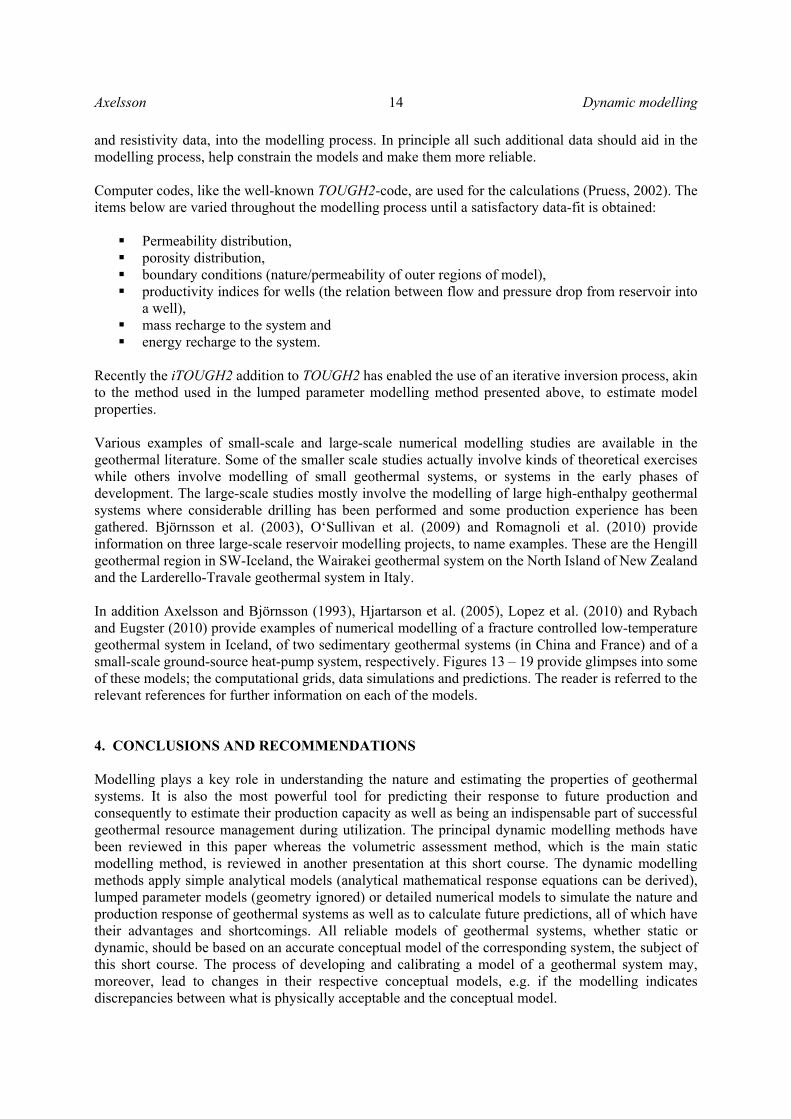
FIGURE 13: A sketch of the computational grid of the most recent numerical reservoir model for the Wairakei geothermal system in New Zealand (O’Sullivan et al., 2009)

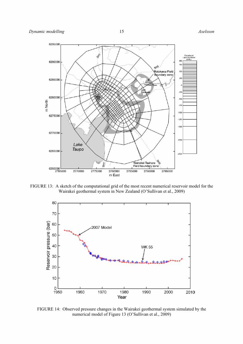
FIGURE 14: Observed pressure changes in the Wairakei geothermal system simulated by the numerical model of Figure 13 (O’Sullivan et al., 2009)

Axelsson 16 Dynamic modelling

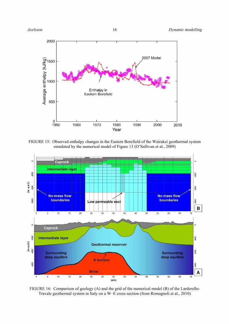
FIGURE 15: Observed enthalpy changes in the Eastern Borefield of the Wairakei geothermal system simulated by the numerical model of Figure 13 (O’Sullivan et al., 2009)

FIGURE 16: Comparison of geology (A) and the grid of the numerical model (B) of the Larderello-Travale geothermal system in Italy on a W–E cross-section (from Romagnoli et al., 2010)

Dynamic modelling 17 Axelsson

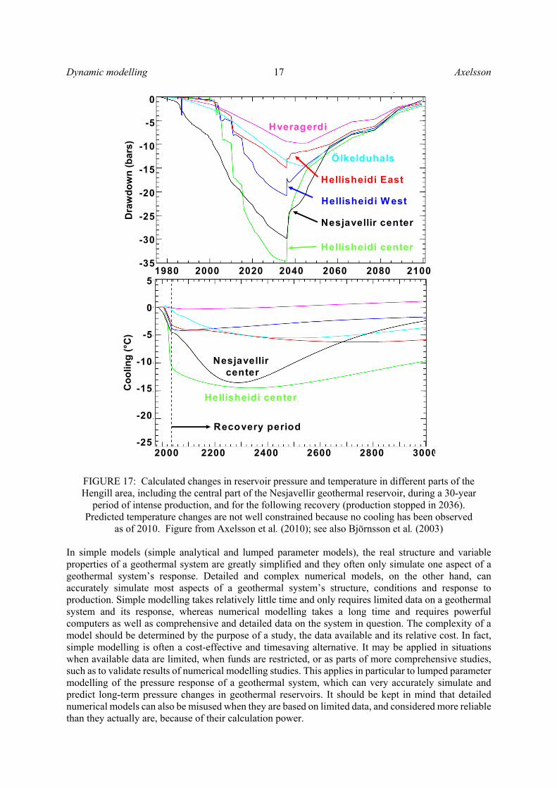
FIGURE 17: Calculated changes in reservoir pressure and temperature in different parts of the Hengill area, including the central part of the Nesjavellir geothermal reservoir, during a 30-year

period of intense production, and for the following recovery (production stopped in 2036). Predicted temperature changes are not well constrained because no cooling has been observed

as of 2010. Figure from Axelsson et al. (2010); see also Björnsson et al. (2003)

In simple models (simple analytical and lumped parameter models), the real structure and variable properties of a geothermal system are greatly simplified and they often only simulate one aspect of a geothermal system’s response. Detailed and complex numerical models, on the other hand, can accurately simulate most aspects of a geothermal system’s structure, conditions and response to production. Simple modelling takes relatively little time and only requires limited data on a geothermal system and its response, whereas numerical modelling takes a long time and requires powerful computers as well as comprehensive and detailed data on the system in question. The complexity of a model should be determined by the purpose of a study, the data available and its relative cost. In fact, simple modelling is often a cost-effective and timesaving alternative. It may be applied in situations when available data are limited, when funds are restricted, or as parts of more comprehensive studies, such as to validate results of numerical modelling studies. This applies in particular to lumped parameter modelling of the pressure response of a geothermal system, which can very accurately simulate and predict long-term pressure changes in geothermal reservoirs. It should be kept in mind that detailed numerical models can also be misused when they are based on limited data, and considered more reliable than they actually are, because of their calculation power.

Hellisheidi center

Nesjavellir center

Hellisheidi W est

Hellisheidi East

Ölkelduhals

Hveragerdi

Hellisheidi center

Nesjavellir center

2000 2200 2400 2600 2800 3000

1980 2000 2020 2040 2060 2080 2100

Co

olin

g(°

C)

Dra

wd

ow

n(b

ars)

5

0

-5

-10

-15

-20

-25

0

-5

-10

-15

-20

-25

-30

-35

Recovery period

Axelsson 18 Dynamic modelling

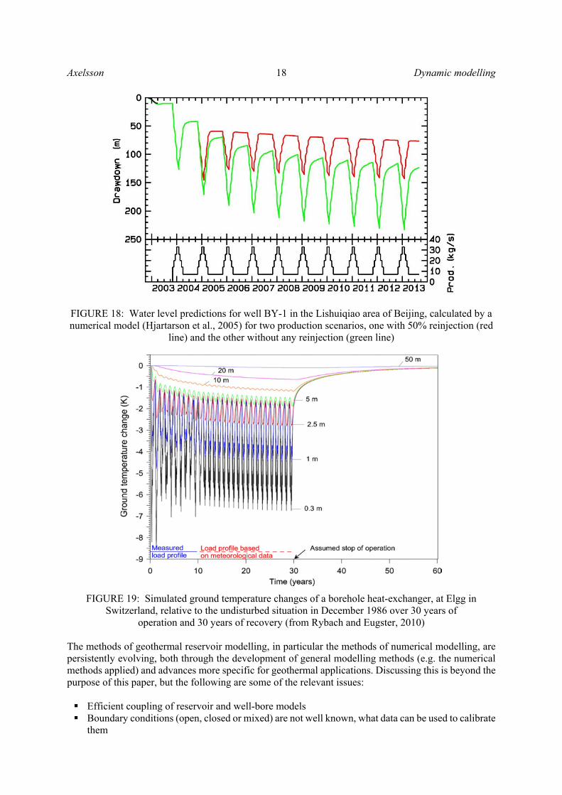
FIGURE 18: Water level predictions for well BY-1 in the Lishuiqiao area of Beijing, calculated by a numerical model (Hjartarson et al., 2005) for two production scenarios, one with 50% reinjection (red

line) and the other without any reinjection (green line)

FIGURE 19: Simulated ground temperature changes of a borehole heat-exchanger, at Elgg in Switzerland, relative to the undisturbed situation in December 1986 over 30 years of

operation and 30 years of recovery (from Rybach and Eugster, 2010) The methods of geothermal reservoir modelling, in particular the methods of numerical modelling, are persistently evolving, both through the development of general modelling methods (e.g. the numerical methods applied) and advances more specific for geothermal applications. Discussing this is beyond the purpose of this paper, but the following are some of the relevant issues: Efficient coupling of reservoir and well-bore models Boundary conditions (open, closed or mixed) are not well known, what data can be used to calibrate

them

Dynamic modelling 19 Axelsson

Nature of bottom boundary, does hot natural recharge e.g. increase during production How to model fractured media accurately and efficiently How to model effect of reinjection, e.g. reservoir and well cooling; difficult to model in detail with

full-scale models How to model production induced cold recharge How to model long-term (~100 yrs) utilization, both production and reinjection effects Modelling of chemical processes such as mineral dissolution and precipitation, which affect

reservoir properties Modelling of high temperature and pressure conditions, even supercritical conditions How should geophysical data (resistivity, seismicity, gravity changes, etc.) be used, in addition to

reservoir data, to calibrate geothermal models Estimating uncertainty in predictions Modelling the deep roots of volcanic systems, i.e. small and large magmatic intrusions.

ACKNOWLEDGEMENTS The author would like to acknowledge numerous colleagues for fruitful discussions and cooperation during the last two – three decades or so, on different aspects of geothermal system modelling, in particular the late Gudmundur Bödvarsson, who was a genuine pioneer in numerical reservoir model-ling. The late Gunnar Bödvarsson, a true grandfather of geothermal reservoir science, proposed the method of lumped parameter modelling discussed above. The relevant geothermal utilities and power companies are also acknowledged for allowing publication of the case-history data presented.

REFERENCES Arnaldsson, A., Gylfadóttir, S. S., Halldórsdóttir, S., Axelsson, G., Mwarania, F., Koech, V., Mbithi, U., and Ouma, P. (2013), “Detailed Numerical Model of the Greater Olkaria Geothermal Area, Kenya”, Proceedings of the 38th Workshop on Geothermal Reservoir Engineering, Stanford University, California, USA. Axelsson, G., 2013: Geothermal well testing. Proceedings of the “Short Course on Conceptual Modelling of Geothermal Systems”, organized by UNU-GTP and LaGeo, Santa Tecla, El Salvador. Axelsson, G., 2012: The Physics of Geothermal Energy. In: Sayigh A, (ed.) Comprehensive Renewable Energy, 7, Elsevier, Oxford, 3–50. Axelsson, G., 2011: Using long case histories to study hydrothermal renewability and sustainable utilization. Geothermal Resources Council Transactions, 35, 1393–1400. Axelsson, G., 2010: Sustainable geothermal utilization – Case histories, definitions, research issues and modelling. Geothermics, 39, 283–291. Axelsson, G., 2008a: Production capacity of geothermal systems. Proceedings of the Workshop for Decision Makers on the Direct Heating Use of Geothermal Resources in Asia, organized by UNU-GTP, TBLRREM and TBGMED, Tianjin, China, 14 pp. Axelsson, G., 2008b: Management of geothermal resources. Proceedings of the Workshop for Decision Makers on the Direct Heating Use of Geothermal Resources in Asia, organized by UNU-GTP, TBLRREM and TBGMED, Tianjin, China, 15 pp.

Axelsson 20 Dynamic modelling

Axelsson, G., and Steingrímsson, B., 2012: Logging, testing and monitoring geothermal wells. Proceedings of the “Short Course on Geothermal Development and Geothermal Wells”, UNU-GTP and LaGeo, Santa Tecla, El Salvador, 20 pp. Axelsson, G., and Gunnlaugsson, E. (convenors), 2000: Long-term monitoring of high- and low-enthalpy fields under exploitation. International Geothermal Association, World Geothermal Congress 2000 Short Course, Kokonoe, Kyushu District, Japan, 226 pp. Axelsson, G., and Björnsson, G., 1993: Detailed Three-Dimensional Modeling of the Botn Hydrothermal System in N-Iceland. Proceedings of the 18th Workshop on Geothermal Reservoir Engineering, Stanford University, California, USA, 159–166. Axelsson, G., Bromley, C., Mongillo, M., and Rybach, L., 2010: The sustainability task of the International Energy Agency’s Geothermal Implementing Agreement. Proceedings World Geothermal Congress 2010, Bali, Indonesia, 8 pp. Axelsson G., Björnsson, G., and Quijano, J., 2005: Reliability of lumped parameter modelling of pressure changes in geothermal reservoirs. Proceedings World Geothermal Congress 2005, Antalya, Turkey, 8 pp. Bertani, R., 2010: Geothermal power generation in the world – 2005–2010 update report. Proceedings World Geothermal Congress 2010, Bali, Indonesia, 41 pp. Bödvarsson, G. S. and Witherspoon, P., 1989: Geothermal reservoir engineering. Part I. Geothermal Science and Technology, 2, 1-68. Bödvarsson G. S., Pruess, K., and Lippmann, M. J., 1986: Modeling of geothermal systems. J. Pet. Tech., 38, 1007–1021. Björnsson, G., Hjartarson, A., Bödvarsson, G. S., and Steingrímsson, B., 2003: Development of a 3-D geothermal reservoir model for the greater Hengill volcano in SW-Iceland. Proceedings of the TOUGH Symposium 2003, Berkeley, CA, USA, 12 pp. Björnsson, G., Axelsson, G. and Flóvenz, Ó. G., 1994: Feasibility study for the Thelamork low-temperature system in N-Iceland. Proceedings 19th Workshop on Geothermal Reservoir Engineering, Stanford University, California, USA, 5-13. Carslaw, H.W. and J.C. Jaeger, 1959: Conduction of Heat in Solids. Second Edition, Claredon Press, Oxford, 403 pp Grant, M.A., and Bixley, P.F., 2011: Geothermal reservoir engineering – Second edition. Academic Press, Burlington, USA, 359 pp. Hjartarson, A., Axelsson, G. and Xu, Y., 2005: Production potential assessment of the low-temperature sedimentary geothermal reservoir in Lishuiqiao, Beijing, P.R. of China, based on a 3-D numerical simulation study. Proceedings World Geothermal Congress 2005, Antalya, Turkey, April, 12 pp. Jacobo, P., and Montalvo, F., 2013: Chemical response monitoring during production. Proceedings of the “Short Course on Conceptual Modelling of Geothermal Systems”, organized by UNU-GTP and LaGeo, Santa Tecla, El Salvador. Lopez, S., Hamm, V., Le Brun, M., Schaper, L., Boissier, F., Cotiche, C., and Giuglaris, E., 2010: 40 years of Dogger aquifer management in Ile-de-France, Paris Basin, France. Geothermics, 39, 339–356.

Dynamic modelling 21 Axelsson

Lund, J. W., Freeston, D. H., and Boyd, T. L., 2010: Direct utilization of geothermal energy – 2010 worldwide review. Proceedings World Geothermal Congress 2010, Bali, Indonesia, 23 pp. Monterrosa, M. E., and Axelsson, G., 2013: Reservoir response monitoring during production. Proceedings of the “Short Course on Conceptual Modelling of Geothermal Systems”, organized by UNU-GTP and LaGeo, Santa Tecla, El Salvador, 12pp. Muffler, L. P. J. and Cataldi, R., 1978: Methods for regional assessment of geothermal resources. Geothermics, 7, 53-89. Onur, M., Sarak, H., Tureyen, O. I., Cinar, M., and Satman, A., 2008: A new non-isothermal lumped-parameter model for low temperature, liquid dominated geothermal reservoirs and its applications. Proceedings of the 33rd Workshop on Geothermal Reservoir Engineering, Stanford University, California, USA, 10 pp. O’Sullivan, M.J., Yeh, A. and Mannington, W. I., 2009: A history of numerical modelling of the Wairakei geothermal field. Geothermics, 38, 155–168. O’Sullivan M. J., Pruess, K., and Lippmann, M. J., 2001: State of the art of geothermal reservoir simulation. Geothermics, 30, 395–429. Pruess K., 2002: Mathematical modelling of fluid flow and heat transfer in geothermal systems. An introduction in five lectures. United Nations University Geothermal Training Programme, Report 3, Reykjavík, 84 pp. Romagnoli, P., Arias, A., Barelli, A., Cei, M., and Casini, M., 2010: An updated numerical model of the Larderello–Travale geothermal system, Italy. Geothermics, 39, 292–313. Rybach, L., and Eugster, W., 2010: Sustainability aspects of geothermal heat pump operation, with experience from Switzerland. Geothermics, 39, 365–369. Rybach, L. and Muffler, L. P. J., 1981: Geothermal systems: Principles and case histories. John Wiley, Chichester, 359 pp. Saemundsson, K., Axelsson, G., and Steingrímsson, B., 2009: Geothermal systems in global perspective. Proceedings of a Short Course on Surface Exploration for Geothermal Resources, organized by UNU-GTP and LaGeo, San Salvador, El Salvador, 16 pp. Sarak, H., Korkmaz, E. D., Onur, M., and Satman, A., 2005: Problems in the use of lumped parameter reservoir models for low-temperature geothermal fields. Proceedings of the World Geothermal Con-gress 2005, Antalya, Turkey, 9 pp. Sarmiento, Z.F., and Björnsson, G., 2007: Reliability of early modelling studies for high-temperature reservoirs in Iceland and the Philippines. Proceedings of the 32nd Workshop on Geothermal Reservoir Engineering, Stanford University, California, USA, 12 pp. Sarmiento, Z. F., Steingrímsson, B., and Axelsson, G., 2013: Volumetric assessment of geothermal resources. Proceedings of the “Short Course on Conceptual Modelling of Geothermal Systems”, organized by UNU-GTP and LaGeo, Santa Tecla, El Salvador, 15 pp. Stefánsson, V., 2005: World geothermal assessment. Proceedings World Geothermal Congress 2005, Antalya, Turkey, 5 pp.