340 VOLUME 20 | NUMBER 3 | MARCH 2017 nature neuroscience

r e v i e w f o c u s o n H u M A n B R A I n M A P P I n G

The origin of spikes in single neurons was essentially solved by the Nobel-prize winning Hodgkin–Huxley model developed in the 1950s. Drawing directly from detailed neurophysiological recordings of the squid giant axon, this model ascribes the origin of spikes to the interaction of fast depolarizing and slow hyperpolarizing currents, expressed in precise mathematical form1. While research into the computational properties of spikes has flourished, movement and per-ception do not typically arise from the spikes of single neurons but by the collective behavior of many cortical, thalamic and spinal neurons in large-scale systems of the brain2,3. Moreover, macroscopic func-tional imaging data such as functional magnetic resonance imaging (fMRI) and electroencephalography (EEG) reflect the collective activ-ity of thousands of neurons4. As yet, there no broadly accepted math-ematical theory for the collective activity of neuronal populations. Traditionally, the analysis of cognitive and functional neuroimaging data has thus largely proceeded without formal biophysical models of the underlying large-scale neuronal activity.

Is such a macroscopic model conceivable in neuroscience, and if so, where are the guideposts? There are many branches of science—magnetism, fluid dynamics, ecology—where observed phenomena reflect collective behavior and not that of individual units. Research in these fields is grounded in precise mathematical laws that govern macroscopic variables such as magnetic fields, fluid flow and popu-lation dynamics5. These laws provide a framework for integrating, explaining and predicting empirical data. Are the collective dynamics of neurons amenable to the ‘mean field’ approaches that underpin these fields?

There do, in fact, exist mean field neural models6–8. Their origin also dates back half a century, to the same type of detailed empiri-cal and theoretical work that characterized the development of the

Hodgkin–Huxley model9. Such models do not describe the behav-ior of individual spiking neurons, but rather the collective action of populations of neurons10. These models have found broad success in modeling seizures11, encephalopathies12,13, sleep14, anesthesia15, rest-ing-state brain networks16,17 and the human alpha rhythm18,19, and as a tool for multimodal data fusion20. Technical advances in model inversion (estimating the likelihood and parameters of a model from empirical data) place mean field models within reach of widespread application to cognitive neuroscience21.

Yet the penetration of dynamic models of large-scale brain activ-ity into mainstream neuroscience has been slow, and they may be unknown to many neuroscientists. Some of the reasons are technical: testing the predictions of these models is challenging. Other reasons may be historical and cultural: neuroscience research has historically prided itself on a very detailed description of individual neurons, their biological components and the computational properties of their spikes. Several large international projects aim to capture these very details through brute-force modeling of large numbers of neurons. To many neuroscientists, a mean field approach discards all of the cell- and circuit-specific information that has been carefully curated.

Models of collective neuronal activity can be crucial to an under-standing of perception and behavior, as well as the determinants of large-scale neuroimaging data. Such models also have their caveats, both technically (limiting their immediate utility) and conceptually (placing bounds on their ultimate utility). This review provides a didactic introduction to dynamic models of large-scale brain activity, from the tenets of the underlying theory to challenges, controversies and recent breakthroughs.

Dynamic models of brain activity: core conceptsDynamical systems theory. Dynamical systems theory originated in the 1600s with Newton and Leibniz, who developed calculus to study celestial mechanics—the motion of the stars and planets. At the heart of this theory are differential equations that express the temporal dynamics of a system’s state variables according to the physi-cal laws governing the system (see Box 1). For planetary motion, the state variables correspond to the position and velocity of the planets.

1QIMR Berghofer Medical Research Institute, Herston, Queensland, Australia. 2Metro North Mental Health Service, Herston, Queensland, Australia. Correspondence should be addressed to M.B. (michael.breakspear@qimrberghofer.edu.au).

Received 15 October 2016; accepted 6 January 2017; published online 23 February 2017; doi:10.1038/nn.4497

Dynamic models of large-scale brain activityMichael Breakspear1,2

Movement, cognition and perception arise from the collective activity of neurons within cortical circuits and across large-scale systems of the brain. While the causes of single neuron spikes have been understood for decades, the processes that support collective neural behavior in large-scale cortical systems are less clear and have been at times the subject of contention. Modeling large-scale brain activity with nonlinear dynamical systems theory allows the integration of experimental data from multiple modalities into a common framework that facilitates prediction, testing and possible refutation. This work reviews the core assumptions that underlie this computational approach, the methodological framework that fosters the translation of theory into the laboratory, and the emerging body of supporting evidence. While substantial challenges remain, evidence supports the view that collective, nonlinear dynamics are central to adaptive cortical activity. Likewise, aberrant dynamic processes appear to underlie a number of brain disorders.

© 2

017

Nat

ure

Am

eric

a, In

c., p

art

of

Sp

rin

ger

Nat

ure

. All

rig

hts

res

erve

d.

nature neuroscience VOLUME 20 | NUMBER 3 | MARCH 2017 341

The differential equations in classical mechanics arise from Newton’s second law. For neural dynamics, such as the Hodgkin–Huxley model, the state variables consist of the membrane potential and ion channel conductances. The differential equations are derived from the bio-physics of ion flow through voltage-gated channels, the conversion of the membrane potential into a firing rate and other biophysical properties of neurons1 and neural populations10,22.

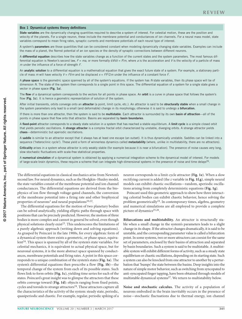
The differential equations for the motion of two planetary bodies can be solved analytically, yielding elliptic paths through space with positions that can be precisely predicted. However, the motion of three bodies is more complex and cannot in general be solved, even though physical solutions clearly exist23. This underscores the limitations of a purely algebraic approach (writing down and solving equations). As grasped by Poincaré in the late 1900s, for every algebraic form of a dynamical system there exists a geometric, or phase space, equiva-lent24. This space is spanned by all of the system’s state variables. For celestial mechanics, it is equivalent to actual physical space, but for neuronal systems, it is the more abstract space spanned by conduct-ances, membrane potentials and firing rates. A point in this space cor-responds to a unique combination of the system’s states (Fig. 1a). The system’s differential equations then prescribe a flow (Fig. 1b)—the temporal change of the system from each of its possible states. Such flows link to form orbits (Fig. 1c), yielding time series for each of the states. Poincaré’s great insight was to glimpse the attractors that these orbits converge toward (Fig. 1d): objects ranging from fixed points, cycles and toroids to strange attractors24. These attractors capture all the characteristics of the activity of the system: steady state, periodic, quasiperiodic and chaotic. For example, regular, periodic spiking of a

neuron corresponds to a limit cycle attractor (Fig. 1e). When a slow rectifying current is added (the z variable in Fig. 1f,g), simple neural models can exhibit chaotic oscillations—random, aperiodic oscilla-tions arising from completely deterministic equations (Fig. 1g).

Poincaré used this geometric approach to show how three interact-ing celestial bodies can exhibit chaotic behavior, hence solving the problem geometrically24. In contemporary times, algebra, geometry and numerical simulations are all employed to provide a complete picture of dynamics25,26.

Bifurcations and multistability. An attractor is structurally sta-ble when a small change in the system’s parameters leads to a slight change in its shape. If the attractor changes dramatically, it is said to be unstable, and the corresponding parameter value is called a bifurcation point. In some systems, two or more attractors can coexist for the same set of parameters, enclosed by their basins of attraction and separated by basin boundaries. Such a system is said to be multistable. A multist-able system will exhibit different forms of activity, such as a steady state equilibrium or chaotic oscillations, depending on its starting state. Such a system can also be knocked from one attractor to another by a pertur-bation that ‘bumps’ the state between the basins. Deep insights into the nature of simple motor behavior, such as switching from syncopated to anti-syncopated finger tapping, have been obtained through models of multistable dynamical systems27. We return to multistability below.

Noise and stochastic calculus. The activity of a population of neurons embodied in the brain inevitably occurs in the presence of noise—stochastic fluctuations due to thermal energy, ion channel

Box 1 Dynamical systems theory definitions State variables are the dynamically changing quantities required to describe a system of interest. For celestial motion, these are the position and velocity of the planets. For a single neuron, these include the membrane potential and conductances of ion channels. For a neural mass model, state variables correspond to mean firing rates, synaptic currents and membrane potentials of each neural type of interest.

A system’s parameters are those quantities that can be considered constant when modeling dynamically changing state variables. Examples can include the mass of a planet, the Nernst potential of an ion species or the density of synaptic connections between different neurons.

A differential equation describes how the state variables change as a function of the current states and the system parameters. The most famous dif-ferential equation is Newton’s second law, F = ma, or more formally dV/dt = F/m, where a is the acceleration and V is the velocity of a particle of mass m under the influence of a force of strength F.

An analytic solution to a differential equation is a mathematical equation that gives the exact future state of a system. For example, a stationary parti-cle of mass m will have velocity V = Ft/m and be displaced x = Ft2/2m under the influence of a constant force F.

A phase space is the geometric space spanned by all of the system’s equations. If the system has N state variables, then its phase space will be of dimension N. The state of the system then corresponds to a single point in this space. The differential equation of a system for a single state gives a vector in phase space (Fig. 1a).

The flow of a dynamical system corresponds to the vectors for all points in phase space. An orbit is a curve in phase space that follows the system’s flow (Fig. 1c). It is hence a geometric representation of solution of the system.

After initial transients, orbits converge onto an attractor (a point, limit cycle, etc.). An attractor is said to be structurally stable when a small change in the system parameters only lead to a small (and deformable) change in its morphology; otherwise it is said to undergo a bifurcation.

If there is more than one attractor, then the system is said to be multistable. Each attractor is surrounded by its own basin of attraction—all of the points in phase space that flow onto that attractor. Basins are separated by basin boundaries.

A fixed-point attractor corresponds to a steady state solution in a system that has reached a stable equilibrium. A limit cycle is a simple closed orbit that yields periodic oscillations. A strange attractor is a complex fractal orbit characterized by unstable, diverging orbits. A strange attractor yields chaos—deterministic but aperiodic oscillations.

A saddle is similar to an attractor except that it always has at least one escape (an outset). It is thus dynamically unstable. Saddles can be linked into a sequence (‘heteroclinic cycle’). These yield a form of winnerless dynamics called metastability (where, unlike in multistability, there are no attractors).

Criticality arises in a system whose attractor is only weakly stable (for example because it is near a bifurcation). The presence of noise causes very long, slow stochastic fluctuations with scale-free statistical properties.

A numerical simulation of a dynamical system is obtained by applying a numerical integration scheme to the dynamical model of interest. For models of large-scale brain dynamics, these require a scheme that can integrate high-dimensional systems in the presence of noise and time delays26.

r e v i e w

© 2

017

Nat

ure

Am

eric

a, In

c., p

art

of

Sp

rin

ger

Nat

ure

. All

rig

hts

res

erve

d.

342 VOLUME 20 | NUMBER 3 | MARCH 2017 nature neuroscience

r e v i e w

chattering and irregular synaptic inputs from other neurons28,29. Such fluctuations arise from both internal and external sources. Adding noise to a dynamical system corresponds to adding small perturba-tions to the orbits at each time step. While the mathematics of sto-chastic differential equations is not trivial, the landscape of orbits, attractors and bifurcations still provides guidance30. For example, a stable limit cycle will still yield oscillatory activity, although with fluctuating amplitude and frequency. Noise added to a multistable system can cause erratic switching among the attractors31. While most of the basic theorems of classic calculus were established centuries ago, stochastic calculus emerged with the study of diffusion in the last century (one of Einstein’s contributions) and remains a very active field, thanks in part to efforts to predict financial markets.

Models of large-scale brain dynamics are thus rooted in stochas-tic calculus. Although they may differ in their implementation, they derive from differential equations for pools of spiking neurons with

two key ingredients: a coupling term that represents synaptic interac-tions between neurons and tends to promote synchronization within the ensemble and a stochastic term that tends to disrupt this effect. The resulting ensemble dynamics reflect this mix of nonlinear neural dynam-ics, interneural coupling and noise16,17. We now address the framework that underpins the study of these noisy ensemble dynamics.

Principles of collective neural behaviorSingle-cell spikes are highly nonlinear, but do such nonlinearities appear in macroscopic neuronal activity, and, if so, what processes ‘transport’ nonlinear dynamics across scales32? What is the suitable form for the equation that best describes such collective dynamics? There are a number of ways to address these questions.

The neural ensemble approach. Arguably the simplest approach to this problem is to assume that at large spatial scales, the exact states

Time series

Attractors

Phase space

a b c d

e f g

y

x x x x

yx x x

y y

z z z

f(x,y)

y y y

z z z

x x x

Time (ms) Time (ms) Time (ms)

Figure 1 A dynamical system is defined by a differential equation dX/dt = f(X). Here X is composed of the two state variables x (the cell membrane potential) and y (the conductance of a fast-depolarizing ion channel). (a) The phase space is the geometric space spanned by the state variables: in this case, simply the Cartesian plane composed of axes for x and y. The dynamical system then defines a vector of length and direction given by f(x,y) at each point—that is, for each combination of membrane potential and ion channel conductance. (b) The flow (also called a vector field) is the set of all such vectors and shows how the dynamical system will flow through phase space: here, a distinctive clockwise flow is evident. (c) An orbit is a solution to the flow—a smooth line that is tangent to the flow. (d) Orbits converge onto the attractors, the long-term solutions of the system. Here there is just a single limit cycle attractor (red) reached from many different starting points (other colors). (e–g) By adding a slow recovery variable z (middle), the system can show a simple limit cycle (e, top), corresponding to regular spiking (e, bottom); or a more complex limit cycle (f, top), yielding regular bursting (f, bottom); or a chaotic (strange) attractor (g, top) with irregular spiking (g, bottom) when the time scales of the spiking and recovery variable mix.

© 2

017

Nat

ure

Am

eric

a, In

c., p

art

of

Sp

rin

ger

Nat

ure

. All

rig

hts

res

erve

d.

nature neuroscience VOLUME 20 | NUMBER 3 | MARCH 2017 343

r e v i e w

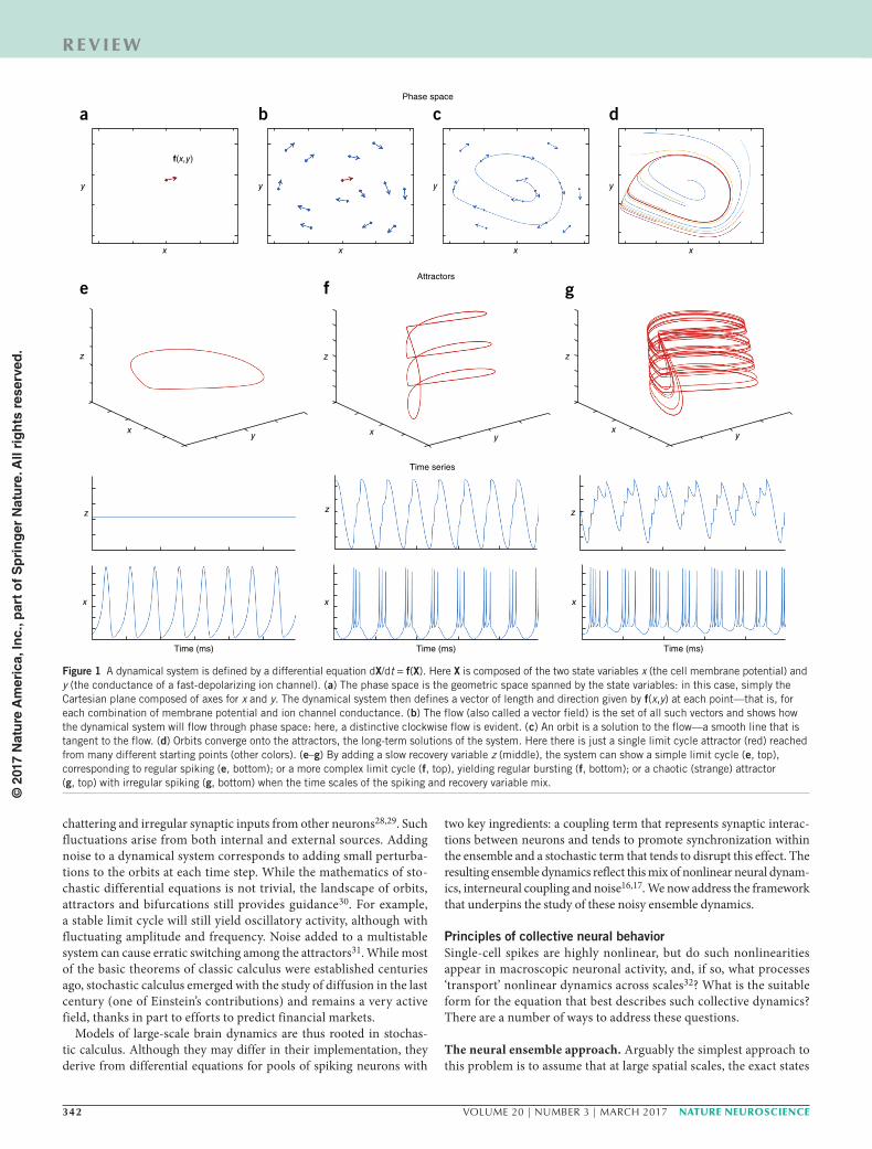
of individual neurons are irrelevant and, moreover, the states of neu-rons across the ensemble are not correlated (Fig. 2a). The central limit theorem states the sum of uncorrelated random processes con-verges to a Gaussian probability distribution, even if the individual processes are highly non-Gaussian (Fig. 2b). According to this ‘dif-fusion approximation’, the entire neural ensemble activity, consisting of highly nonlinear but largely uncorrelated spikes, can be reduced to a standard normal probability distribution possessing simple linear statistics. The activity of such an ensemble of neurons—a patch of cortex—can hence be described by the mean and variance of the fir-ing rate. The mean firing rate reflects the response of the population to its total synaptic inputs and hence drifts up and down in response to increasing or decreasing afferent input33. The variance reflects the dispersion (roughness) of all stochastic effects and will change as the variance of the noise changes.

The equation that describes the dynamics of such a linear, normally distributed ensemble is called the Fokker–Planck equation (FPE). An FPE for a neural ensemble can be analytically derived from simple (integrate and fire) single-neuron models under the assumption that the diffusion approximation holds true34–38. The FPE captures the collective response of a neuronal population to its inputs. Each neuron responds to its own inputs and effectively submits an independent vote to the ‘democratic’ collective. The mean firing rate is essentially

a passive summation of all these responses and encodes the average (the most likely) population-based representation of its inputs. The FPE also describes the dynamics of the population variance, corre-sponding to the precision with which the ensemble response is rep-resented39,40. As the inputs to the ensemble change, the FPE captures the drift (of the mean) and diffusion (change in the variance) of the ensemble activity (Fig. 2c).

The FPE is an analytically achievable representation of how local populations represent their inputs. Individual nonlinearities, local correlations between neurons, and subtle differences within families of neurons are all accommodated by the diffusion approximation. An FPE reduces the thousands of degrees of freedom of a brute-force model of spiking neurons to two variables capturing the mean activ-ity and the dispersion around that mean. Such dimension reduction is at the heart of efforts to move beyond brute-force accounts of the brain41. The Gaussian distribution maximizes the ratio of the entropy to the variance of any distribution; the potential information content of an ensemble of neurons is thus at its upper limit when it obeys a FPE. The linear FPE may therefore be seen as the starting point for large-scale models of neuronal systems.

When the statistics of a local ensemble are Gaussian, the stand-ard FPE represents a powerful and parsimonious way of balancing complexity with tractability. However, converging evidence from a variety of neuronal recordings suggests that although the spatial42 and temporal12,43,44 statistics of neural population activity do con-form to simple probability distributions, these are often heavy-tailed and not Gaussian. Such heavy tails correspond to the occurrence of synchronized bursts of activity that violate the diffusion assumption (Fig. 2d). In brief, erratic bursts of synchronization transport cor-related states from the micro-scale to the macroscopic scale, causing non-Gaussian fluctuations (Fig. 2e and Box 2). What are the options for modeling heavy-tailed neural ensembles? Reassuringly, when the statistics obey other simple probability distributions (such as a power law), there do exist well defined and tractable (nonlinear or fractional) FPEs. The theoretical armory of random field theory can be adapted to these well-behaved non-Gaussian scenarios. These more general FPEs are hence potentially very useful for modeling neural ensembles with strong correlations and heavy-tailed statistics. However, while this is an active area in theoretical physics, it is a relatively unexplored avenue in neuroscience. We thus consider other possibilities below.

Neural mass models. In the presence of strong coherence, it may be reasonable to assume that the ensemble activity is sufficiently close to the mean that the variance can be discarded. This reduces the number of dimensions to one and allows multiple interacting local popula-tions, such as excitatory and inhibitory neurons in different layers of cortex, to be modeled by a small number of equations, each describ-ing the mean activity of a neural population45,46. This mass-action approach is at the heart of neural mass models (NMMs)10.

NMMs come in several flavors. One class is derived by assuming that coherence between neurons is so strong that the dynamics of the entire ensemble of neurons resembles that of each single neuron. Accordingly, the mean ensemble activity is modeled with the same conductance-based model as used in single-neuron models. This assumption is relaxed somewhat by replacing the all-or-nothing fir-ing of individual neurons with a sigmoid-shaped activation function that maps the average membrane potential to the mean firing rate (Fig. 3a). The breadth of this sigmoid function implicitly incorporates the variance of individual neural thresholds, as well as the dispersion of their states47. The central difference between such NMMs and the FPE is that the variance is constant in NMMs whereas it is free to vary

a

b

Cor

rela

tion

Subsystem separation

Pro

ba

bili

ty

Pro

ba

bili

ty

Mean firing rate

ec

Pro

ba

bili

ty

d

Cor

rela

tion

Subsystem separation

Mean firing rate

Mean firing rate

Figure 2 Principles of the neuronal ensemble reduction. (a) Complex spatial systems composed of interacting components, such as human cortical columns, are characterized by interactions that weaken with distance. (b) If the resulting correlations decay quickly compared to the size of the system, the statistics of the system converge toward a Gaussian distribution (inset), even if the statistics within the individual components are highly non-Gaussian. (c) The Fokker–Planck equation describes how the statistics passively change when the inputs and strength of stochastic fluctuations change. Here the inputs increase and the noise becomes less influential. The mean rate drifts up and the ensemble distribution becomes more precise as we move in the direction of the arrow. (d) If correlations within the system become stronger—for example, owing to synchrony—the correlation length diverges toward the size of the system in the direction of the arrow toward the blue curve. The assumptions underlying the diffusion approximation may not be met. (e) If strong ensemble correlations exist, the statistics may converge toward a non-Gaussian distribution (blue curve). Typical fluctuations shrink toward the mean (and hence the distribution becomes more tent-like), but the left and right tails (extremes) become fatter, corresponding to infrequent but high-amplitude, synchronous fluctuations.

© 2

017

Nat

ure

Am

eric

a, In

c., p

art

of

Sp

rin

ger

Nat

ure

. All

rig

hts

res

erve

d.

344 VOLUME 20 | NUMBER 3 | MARCH 2017 nature neuroscience

r e v i e w

in the FPE. NMMs of this kind often consist of a conductance-based spiking excitatory neuron pool coupled to a passive local inhibitory pool and can exhibit steady state, periodic or chaotic oscillations48,49. This last case arises through the mixing of fast and slow time scales.

A second way to construct NMMs adopts the approach of Hodgkin and Huxley—namely, using careful empirical observations to under-stand and model the response of the system to its inputs. Hodgkin and Huxley carefully observed the conductance of a single axon in response to changes in the membrane potential. Similarly, early neural mass models were derived from careful observation of the collective response of a neural population (the rabbit olfactory bulb) to changes in driving inputs9. This approach respects the notion that complex systems can exhibit specific rules at different levels of organization and that large-scale activity may hence be more than the sum of its parts. Empirically informed NMMs include the Wilson–Cowan22 and Jansen–Rit45 models. There also exist hybrid methods that combine theoretical treatments of population dynamics with empirical synap-tic and input-response functions50–52.

Large-scale brain dynamicsNetworks of neural masses. A NMM describes a local population of interacting neurons, such as pyramidal and inhibitory cells. Despite the dimension reduction achieved, there still exist several orders of magnitude between a small patch of cortex and the large-scale systems that support brain function. Bridging these scales can be achieved by coupling an ensemble of NMMs into mesoscopic circuits10,53 and macroscopic systems54. Dynamics within each neuronal population node (that is, each NMM) consequently reflects the local population activity plus influences from distal regions (other nodes) and sto-chastic fluctuations (Fig. 3b). Such large-scale brain network models (BNMs) are a multiscale ‘ensemble of ensembles’, with distinct prin-ciples of organization operating at different scales55.

The coupling of NMMs into a larger system should be informed by anatomical connectivity; that is, the connectome. Suitable connec-tomic data can be obtained from collations of invasive tracing studies, such as the primate CoCoMac56 or recent detailed rodent connec-tomes57. For human brain models, large-scale connectivity data can be inferred from diffusion MRI-based tractography. The modeling

community has employed both of these options. The resulting whole-brain dynamic models differ in the choice of the local NMM, the treatment of conduction delays between nodes and the role of chaotic versus stochastic dynamics16,17,58. This is a powerful approach that integrates decades of work on NMMs with the study of complex brain networks26,59. The application of BNMs to resting-state fMRI data is a very active area that we review below.

Neural field models. BNMs treat the cortex as a discrete network of dynamic nodes coupled through the connectome. But at macroscopic scales, the cortex may also be treated as a continuous sheet composed of dense short-range connections that quickly (exponentially) dimin-ish in number with inter-areal distance57. Large-scale neural mod-els that treat the cortex as a continuous sheet—neural field models (NFMs)—draw on well-established field models in other complex sys-tems and have a rich history in computational neuroscience60,61. The most general formulations use a combination of differential equations (for the treatment of time) and integrals (for the treatment of spatial coupling and time delays)22,62. For biologically realistic assumptions regarding the synaptic kernel (the local connectivity footprint), it is possible to write this as a wave equation—a partial differential equation with temporal and spatial derivatives6–8,63. Additional ana-tomical features, such as corticothalamic loops18 and patchy connec-tivity64,65, can also be incorporated (Fig. 3c). NFMs have provided insights into the contribution of large-scale cortical systems to cortical rhythms18, transitions to and from sleep14, epileptic seizures11,18 and evoked potentials66. The excited modes of a whole brain neural field model—the small number of spatiotemporal patterns that capture most of the system’s energy—show a striking match to the canonical resting-state networks67. NFMs are, at their heart, nonlinear wave models60. They thus promise to account for the broad spectrum of wave-like empirical data, such as the propagating fronts of oscillatory activity observed in sensory and motor cortices68–70.

While detailed node-to-node network connections pervade accounts of the human connectome, it is also true that coupling between adjacent patches of cortex is stronger than the long-range connections that integrate cortical circuits into large-scale systems71. Recent highly resolved tracer- and tractography-based connectomes

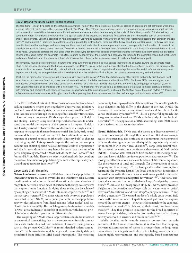
Box 2 Beyond the linear Fokker-Planck equation The traditional (linear) FPE rests on the diffusion assumption, namely that the activities of neurons or groups of neurons are not correlated when mea-sured at different points across the system of interest (Fig. 2a–c). The FPE can accommodate spike correlations among neurons within small circuits, but requires that correlations between more distant neurons are weak and disappear entirely at the scale of the entire system36. Put alternatively, the correlation length is considerably shorter than the spatial scale of the system, and ensemble fluctuations are thus the passive sum of uncorrelated smaller scale events. Does this assumption hold empirically? Converging evidence from a variety of neuronal recordings suggests that although the spa-tial42,43 and temporal120 statistics do conform to simple probability distributions, these are often heavy-tailed and not Gaussian. The heavy tails arise from fluctuations that are larger and more frequent than permitted under the diffusion approximation and correspond to the formation of transient but nontrivial correlations among distant neurons. Correlations among neurons arise from synchronization either in their firing or in the modulations of their firing rates. Long-range correlations thus arise when the underlying tendency for coupled dynamical systems to synchronize overwhelms the disruptive effects of the noise within the ensemble (Fig. 2d). Neurons no longer filter their inputs and passively contribute to the ensemble mean, but synchronize to dynamic feedback from the mean, which acts to increase the coherence (as when voters react to real-time feedback of a poll).

The dynamic, multiscale recruitment of neurons into large synchronous ensembles thus causes their states to converge toward the ensemble mean (that is, the variance shrinks and the kurtosis increases; Fig. 2e)147. Owing to the resulting statistical redundancy between neurons, the entropy of the ensemble thus decreases. Paradoxically, this reduction in entropy may confer a computational advantage because the useful information in a system depends on not only the entropy (information diversity) but also the reliability148: that is, on the balance between entropy and redundancy.

What are the options for modeling neural ensembles with heavy-tailed activity? When the statistics obey other simple probability distributions (such as a bimodal or power-law function), there do exist well-defined and tractable nonlinear and fractional FPEs. Nonlinear FPEs contain higher order interactions between the mean and noise terms. A system (such as a financial market) that becomes more volatile during high throughput (such as high-volume trading) can be modeled with a nonlinear FPE. The fractional FPE arises from a generalization of calculus to model stochastic systems with memory and persistent long-range correlations—as observed widely in neuroscience, such as in the fluctuations of the alpha rhythm149. It rests on a deep reformulation of calculus. Although conceptually appealing, fractional calculus has thus far had few applications in neuroscience150.

© 2

017

Nat

ure

Am

eric

a, In

c., p

art

of

Sp

rin

ger

Nat

ure

. All

rig

hts

res

erve

d.

nature neuroscience VOLUME 20 | NUMBER 3 | MARCH 2017 345

r e v i e w

provide converging evidence for a synaptic footprint that is largely invariant (similar throughout the cortex), creating a smooth con-nectivity that is modulated by specific long-range network con-nections57,72. This highlights the geometric attributes of cortical

connectivity and supports the assumptions underlying NFMs. The integration of BNMs and NFMs into a single framework is an active area of research that aims to reconcile the apparently contradictory aspects of these large-scale brain models64,73.

Connectome

Mea

n fir

ing

rate

Mean membrane potential

Cell threshold

Pro

babi

lity

a

cb Brain network models

y

x

z

Neural mass models

Neural field models

Excitatory cell Excitatory axon

Inhibitory cellInhibitory axon

Non-specific connection

EEG data Neural field model

Wave of activity

Time (s)Time (s)Spatiotemporal brain dynamics

Sca

lp e

lect

rode

s

Vir

tual

ele

ctro

des

i

ii

iii

iv

v

vi

t = 2 ms t = 4 ms t = 6 ms

Pyramidal cell

Inhibitory cell

Excitatory (efferent)

Inhibitory connection

Excitatory (afferent)

Figure 3 Models of large-scale brain dynamics. (a) Neural mass models (NMMs) are obtained by taking the average states in all neurons of each class (pyramidal, inhibitory) in a local population, here a cortical column (left). Traditional spiking neural models treat each neuron as an idealized individual unit (center). NMMs go further, reducing the entire population dynamics to a low-dimensional differential equation representing the average states of local interacting neurons (right). The variability in the cell threshold (inset, top right) smooths the all-or-nothing action potential of each neuron into a smooth sigmoidal map between average membrane potential and average firing rate. Integrating this equation yields an attractor for the local dynamics (bottom right). (b) Brain network models (BNMs) are composed by coupling an ensemble of NMMs into a large-scale system (top), with connections informed by the connectome (adapted from G. Roberts, A. Perry, A. Lord, A. Frankland, V. Leung et al., Mol. Psychiatry, in the press). Due to strong short-range connections, BNMs can yield wave patterns (bottom). This example shows a wave traveling diagonally to the right. (c) In a neural field model (NFM), the cortex is treated as a smooth sheet (top) that supports waves of propagating activity (top inset). Neural field models that include a neural mass in the thalamus (bottom inset) yield alpha oscillations with the same spectral properties as those observed in empirical data (bottom; adapted from ref. 11, Oxford University Press).

© 2

017

Nat

ure

Am

eric

a, In

c., p

art

of

Sp

rin

ger

Nat

ure

. All

rig

hts

res

erve

d.

346 VOLUME 20 | NUMBER 3 | MARCH 2017 nature neuroscience

r e v i e w

Large-scale neural activity: empirical findingsModels of large-scale brain dynamics thus derive from detailed, theoretical treatments of neural population dynamics. However, the validity of a dynamic model of the brain is ultimately an empirical question: what is the evidence that such models can explain, pre-dict and unify neurophysiological data? What tools are required to appraise this question?

The rise and fall of chaos theory. For parameter values correspond-ing to high gain and strong synaptic input, neural mass and neural field models yield highly nonlinear dynamics. Limit cycle attractors have been proposed to underlie the brain’s large-scale oscillations, including the alpha22 and beta74 rhythms. Chaotic attractors also arise in NMMs, yielding complex, aperiodic nonlinear oscillations48. The presence of such nonlinear waveforms in macroscopic signals such as EEG would provide compelling support for these models and, more deeply, for the implicit assumption on which they rest: namely, that through synchrony, collective neuronal dynamics retain the nonlin-earities present at the microscopic scale.

Chaotic dynamics arise from unstable nonlinear processes, yielding complex attractors with fractal geometry. In the 1980s, new com-putational algorithms allowed the quantification of these properties in empirical data75,76. The broad appeal of chaos—the emergence of complex dynamics from simple rules—fueled the application of these algorithms to data from diverse systems. As in many fields, large-scale neurophysiological data, acquired during rest77,78, sleep79, cognition80 and seizures81, were subsequently observed to possess the classic hallmarks of chaotic dynamics.

The algorithms for detecting chaos certainly yielded valid results for the theoretical dynamical systems in which they were devel-oped—lengthy time series data obtained by integrating nonlinear systems. Unfortunately, substantial limitations were soon identified in the application of these algorithms to noisy, nonstationary and often relatively brief empirical data. In particular, it was shown that filtered (linear) noise could also yield the numeric values that had been previously associated with chaos82–84. Recognition of these limi-tations led to a reappraisal of prior findings and to more circumspect conclusions regarding the role of simple chaotic dynamics in large-scale neural systems85,86.

In retrospect, the initial application of measures of chaotic dynam-ics to time series data may have reflected a confirmation bias—an implicit objective to show that empirical data are consistent with an appealing theoretical framework. Alternative hypotheses—that the measures of chaos might be generated by filtered linear noise with no further temporal structure, for example—were not systematically tested. The ability to represent the null hypothesis for the values of these measures (representing trivial, nonchaotic fluctuations) was facilitated by the development of resampling algorithms in the early 1990s87,88. These resampling algorithms yield surrogate data of the same length and possessing the same linear properties as the original data but with any putative nonlinear structure destroyed. By deriv-ing the nonlinear metrics from these surrogate data, it is possible to construct the null hypothesis—the expected distribution of values due to trivial linear correlations and finite sample length. Only those empirical data whose measures fall outside this null distribution can be said to possess nonlinear properties such as chaos.

Bifurcations and multistability in human cortex. The reappraisal of nonlinear structure in large-scale neurophysiological data using null hypothesis testing led to a consensus that is more qualified than the early reports of simple chaos. Robust89 and replicated90 analyses

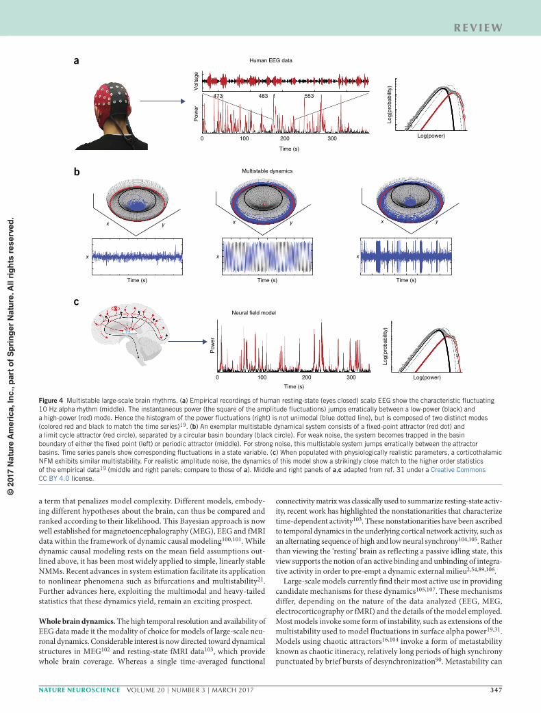
of resting-state EEG data using surrogate data suggest that healthy cortical activity is not chaotic, but rather jumps erratically between a high-amplitude, nonlinear 10 Hz oscillation and low-amplitude fil-tered noise (Fig. 4a)—that is, the resting cortex operates in a regime of multistability consisting of a limit cycle and a fixed point attractor (Fig. 4b)31,91,92. It was later shown that a corticothalamic NFM could yield a multistable attractor landscape in the presence of biophysically plausible corticothalamic feedback. When driven by noise, this model erratically switches between the fixed point and limit cycle, yielding time series data whose spectra and higher statistical properties show close agreement with experimental data (Fig. 4c)19.

The application of null hypothesis testing using surrogate data thus substantially changed our understanding of nonlinear dynamics in healthy cortex. However, the initial reports of sustained nonlinear dynamics during seizures did survive surrogate data testing. That is, the onset of a seizure is thought to correspond to the appearance of sustained high-amplitude nonlinear oscillations, suggesting a bifurca-tion from resting state to a limit cycle or chaotic attractor11,93. Again, this observation is supported by NMMs94,95 and NFMs18, which pre-dict that a bifurcation in the underlying large-scale cortical96 and corticothalamic11 dynamics yields primary generalized seizures. While further challenges remain, observations of multistability in health and of bifurcations in seizures confirm the core assumptions underlying large-scale models: namely, that dynamical processes may occur at the largest scale of the brain and are not passively washed away in the noise.

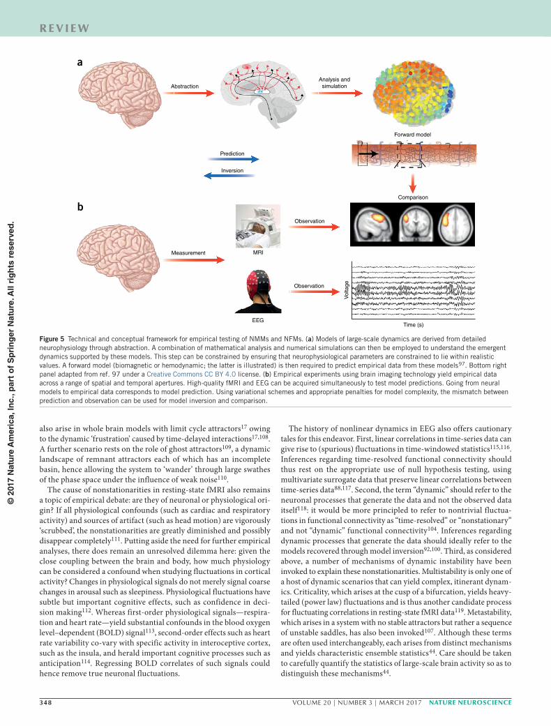
Emerging topics in large-scale neuronal modelsTesting, comparing and refuting models. Surrogate testing of empir-ical data provides an opportunity to confirm or refute the implicit assumptions underlying large-scale neural models. However, fur-ther steps are required to establish the validity of any specific model. Neural models predict the underlying neural states (firing rates, membrane potentials, etc.). While the mass action of these models yields aggregate dynamics that match the spatial apertures of imaging data, the neural states are hidden (not directly observable). Scalp EEG arises from macroscopic ion currents, yielding voltage changes refer-enced to a distal electrode. Biophysically informed forward models are required to understand the mapping from currents in the folded cortex to fluctuating extradural electrocorticographic and scalp EEG potentials. Likewise, spatiotemporal hemodynamic response func-tions are required to map large-scale neural activity to fMRI data97. When combined with measurement noise, these biomagnetic and hemodynamic forward models provide a principled way of testing the predictions of large-scale models of the brain against empirical data. Just as the classic accounts of planetary motion rested on the theory of optics, inference regarding models of large-scale neural activity depend on valid observation models. By allowing prediction of multiple streams of data, each through its own forward model, this approach also permits fusion of multimodal data such as simultane-ously acquired EEG and fMRI20,98,99 (Fig. 5).

The specific predictions of a model also depend on the choice of its parameters: the gain, inputs, strengths of coupling and noise, etc. Fine-tuning by hand is often impractical and lends itself to overfitting; that is, using a complex combination of parameters that are unique to a specific data set and generalize poorly. More technically, model pre-dictions are conditioned on the choice of parameters. Integrating out this dependency can be achieved within a Bayesian framework, which allows estimation of the probability of a model prediction given the likely (prior) distribution of its parameter values. The likelihood of a specific model can then be estimated though inversion by introducing

© 2

017

Nat

ure

Am

eric

a, In

c., p

art

of

Sp

rin

ger

Nat

ure

. All

rig

hts

res

erve

d.

nature neuroscience VOLUME 20 | NUMBER 3 | MARCH 2017 347

r e v i e w

a term that penalizes model complexity. Different models, embody-ing different hypotheses about the brain, can thus be compared and ranked according to their likelihood. This Bayesian approach is now well established for magnetoencephalography (MEG), EEG and fMRI data within the framework of dynamic causal modeling100,101. While dynamic causal modeling rests on the mean field assumptions out-lined above, it has been most widely applied to simple, linearly stable NMMs. Recent advances in system estimation facilitate its application to nonlinear phenomena such as bifurcations and multistability21. Further advances here, exploiting the multimodal and heavy-tailed statistics that these dynamics yield, remain an exciting prospect.

Whole brain dynamics. The high temporal resolution and availability of EEG data made it the modality of choice for models of large-scale neu-ronal dynamics. Considerable interest is now directed toward dynamical structures in MEG102 and resting-state fMRI data103, which provide whole brain coverage. Whereas a single time-averaged functional

connectivity matrix was classically used to summarize resting-state activ-ity, recent work has highlighted the nonstationarities that characterize time-dependent activity103. These nonstationarities have been ascribed to temporal dynamics in the underlying cortical network activity, such as an alternating sequence of high and low neural synchrony104,105. Rather than viewing the ‘resting’ brain as reflecting a passive idling state, this view supports the notion of an active binding and unbinding of integra-tive activity in order to pre-empt a dynamic external milieu2,54,89,106.

Large-scale models currently find their most active use in providing candidate mechanisms for these dynamics105,107. These mechanisms differ, depending on the nature of the data analyzed (EEG, MEG, electrocorticography or fMRI) and the details of the model employed. Most models invoke some form of instability, such as extensions of the multistability used to model fluctuations in surface alpha power19,31. Models using chaotic attractors16,104 invoke a form of metastability known as chaotic itineracy, relatively long periods of high synchrony punctuated by brief bursts of desynchronization90. Metastability can

Time (s)

Pow

erV

olta

ge

0 100 200 300

473 483 ! 553

Log(power)

Log(

prob

abili

ty)

Time (s) Time (s) Time (s)

Time (s)

Pow

er

0 100 200 300 Log(power)Lo

g(pr

obab

ility

)

a

c

Human EEG data

Neural field model

b Multistable dynamics

yx yx yx

xx x

Figure 4 Multistable large-scale brain rhythms. (a) Empirical recordings of human resting-state (eyes closed) scalp EEG show the characteristic fluctuating 10 Hz alpha rhythm (middle). The instantaneous power (the square of the amplitude fluctuations) jumps erratically between a low-power (black) and a high-power (red) mode. Hence the histogram of the power fluctuations (right) is not unimodal (blue dotted line), but is composed of two distinct modes (colored red and black to match the time series)19. (b) An exemplar multistable dynamical system consists of a fixed-point attractor (red dot) and a limit cycle attractor (red circle), separated by a circular basin boundary (black circle). For weak noise, the system becomes trapped in the basin boundary of either the fixed point (left) or periodic attractor (middle). For strong noise, this multistable system jumps erratically between the attractor basins. Time series panels show corresponding fluctuations in a state variable. (c) When populated with physiologically realistic parameters, a corticothalamic NFM exhibits similar multistability. For realistic amplitude noise, the dynamics of this model show a strikingly close match to the higher order statistics of the empirical data19 (middle and right panels; compare to those of a). Middle and right panels of a,c adapted from ref. 31 under a Creative Commons CC BY 4.0 license.

© 2

017

Nat

ure

Am

eric

a, In

c., p

art

of

Sp

rin

ger

Nat

ure

. All

rig

hts

res

erve

d.

348 VOLUME 20 | NUMBER 3 | MARCH 2017 nature neuroscience

r e v i e w

also arise in whole brain models with limit cycle attractors17 owing to the dynamic ‘frustration’ caused by time-delayed interactions17,108. A further scenario rests on the role of ghost attractors109, a dynamic landscape of remnant attractors each of which has an incomplete basin, hence allowing the system to ‘wander’ through large swathes of the phase space under the influence of weak noise110.

The cause of nonstationarities in resting-state fMRI also remains a topic of empirical debate: are they of neuronal or physiological ori-gin? If all physiological confounds (such as cardiac and respiratory activity) and sources of artifact (such as head motion) are vigorously ‘scrubbed’, the nonstationarities are greatly diminished and possibly disappear completely111. Putting aside the need for further empirical analyses, there does remain an unresolved dilemma here: given the close coupling between the brain and body, how much physiology can be considered a confound when studying fluctuations in cortical activity? Changes in physiological signals do not merely signal coarse changes in arousal such as sleepiness. Physiological fluctuations have subtle but important cognitive effects, such as confidence in deci-sion making112. Whereas first-order physiological signals—respira-tion and heart rate—yield substantial confounds in the blood oxygen level–dependent (BOLD) signal113, second-order effects such as heart rate variability co-vary with specific activity in interoceptive cortex, such as the insula, and herald important cognitive processes such as anticipation114. Regressing BOLD correlates of such signals could hence remove true neuronal fluctuations.

The history of nonlinear dynamics in EEG also offers cautionary tales for this endeavor. First, linear correlations in time-series data can give rise to (spurious) fluctuations in time-windowed statistics115,116. Inferences regarding time-resolved functional connectivity should thus rest on the appropriate use of null hypothesis testing, using multivariate surrogate data that preserve linear correlations between time-series data88,117. Second, the term “dynamic” should refer to the neuronal processes that generate the data and not the observed data itself118: it would be more principled to refer to nontrivial fluctua-tions in functional connectivity as “time-resolved” or “nonstationary” and not “dynamic” functional connectivity104. Inferences regarding dynamic processes that generate the data should ideally refer to the models recovered through model inversion92,100. Third, as considered above, a number of mechanisms of dynamic instability have been invoked to explain these nonstationarities. Multistability is only one of a host of dynamic scenarios that can yield complex, itinerant dynam-ics. Criticality, which arises at the cusp of a bifurcation, yields heavy-tailed (power law) fluctuations and is thus another candidate process for fluctuating correlations in resting-state fMRI data119. Metastability, which arises in a system with no stable attractors but rather a sequence of unstable saddles, has also been invoked107. Although these terms are often used interchangeably, each arises from distinct mechanisms and yields characteristic ensemble statistics44. Care should be taken to carefully quantify the statistics of large-scale brain activity so as to distinguish these mechanisms44.

a

b

Forward model

Comparison

Observation

Observation

Prediction

Inversion

EEG

MRI

Analysis andsimulation

Vol

tage

Time (s)

Abstraction

Measurement

Figure 5 Technical and conceptual framework for empirical testing of NMMs and NFMs. (a) Models of large-scale dynamics are derived from detailed neurophysiology through abstraction. A combination of mathematical analysis and numerical simulations can then be employed to understand the emergent dynamics supported by these models. This step can be constrained by ensuring that neurophysiological parameters are constrained to lie within realistic values. A forward model (biomagnetic or hemodynamic; the latter is illustrated) is then required to predict empirical data from these models97. Bottom right panel adapted from ref. 97 under a Creative Commons CC BY 4.0 license. (b) Empirical experiments using brain imaging technology yield empirical data across a range of spatial and temporal apertures. High-quality fMRI and EEG can be acquired simultaneously to test model predictions. Going from neural models to empirical data corresponds to model prediction. Using variational schemes and appropriate penalties for model complexity, the mismatch between prediction and observation can be used for model inversion and comparison.

© 2

017

Nat

ure

Am

eric

a, In

c., p

art

of

Sp

rin

ger

Nat

ure

. All

rig

hts

res

erve

d.

nature neuroscience VOLUME 20 | NUMBER 3 | MARCH 2017 349

r e v i e w

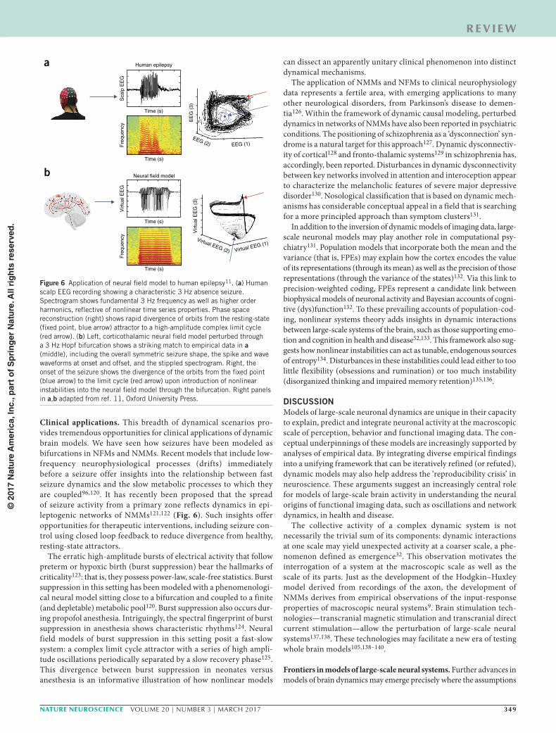
Clinical applications. This breadth of dynamical scenarios pro-vides tremendous opportunities for clinical applications of dynamic brain models. We have seen how seizures have been modeled as bifurcations in NFMs and NMMs. Recent models that include low- frequency neurophysiological processes (drifts) immediately before a seizure offer insights into the relationship between fast seizure dynamics and the slow metabolic processes to which they are coupled96,120. It has recently been proposed that the spread of seizure activity from a primary zone reflects dynamics in epi-leptogenic networks of NMMs121,122 (Fig. 6). Such insights offer opportunities for therapeutic interventions, including seizure con-trol using closed loop feedback to reduce divergence from healthy, resting-state attractors.

The erratic high-amplitude bursts of electrical activity that follow preterm or hypoxic birth (burst suppression) bear the hallmarks of criticality123: that is, they possess power-law, scale-free statistics. Burst suppression in this setting has been modeled with a phenomenologi-cal neural model sitting close to a bifurcation and coupled to a finite (and depletable) metabolic pool120. Burst suppression also occurs dur-ing propofol anesthesia. Intriguingly, the spectral fingerprint of burst suppression in anesthesia shows characteristic rhythms124. Neural field models of burst suppression in this setting posit a fast-slow system: a complex limit cycle attractor with a series of high ampli-tude oscillations periodically separated by a slow recovery phase125. This divergence between burst suppression in neonates versus anesthesia is an informative illustration of how nonlinear models

can dissect an apparently unitary clinical phenomenon into distinct dynamical mechanisms.

The application of NMMs and NFMs to clinical neurophysiology data represents a fertile area, with emerging applications to many other neurological disorders, from Parkinson’s disease to demen-tia126. Within the framework of dynamic causal modeling, perturbed dynamics in networks of NMMs have also been reported in psychiatric conditions. The positioning of schizophrenia as a ‘dysconnection’ syn-drome is a natural target for this approach127. Dynamic dysconnectiv-ity of cortical128 and fronto-thalamic systems129 in schizophrenia has, accordingly, been reported. Disturbances in dynamic dysconnectivity between key networks involved in attention and interoception appear to characterize the melancholic features of severe major depressive disorder130. Nosological classification that is based on dynamic mech-anisms has considerable conceptual appeal in a field that is searching for a more principled approach than symptom clusters131.

In addition to the inversion of dynamic models of imaging data, large-scale neuronal models may play another role in computational psy-chiatry131. Population models that incorporate both the mean and the variance (that is, FPEs) may explain how the cortex encodes the value of its representations (through its mean) as well as the precision of those representations (through the variance of the states)132. Via this link to precision-weighted coding, FPEs represent a candidate link between biophysical models of neuronal activity and Bayesian accounts of cogni-tive (dys)function132. To these prevailing accounts of population-cod-ing, nonlinear systems theory adds insights in dynamic interactions between large-scale systems of the brain, such as those supporting emo-tion and cognition in health and disease52,133. This framework also sug-gests how nonlinear instabilities can act as tunable, endogenous sources of entropy134. Disturbances in these instabilities could lead either to too little flexibility (obsessions and rumination) or too much instability (disorganized thinking and impaired memory retention)135,136.

DiSCuSSionModels of large-scale neuronal dynamics are unique in their capacity to explain, predict and integrate neuronal activity at the macroscopic scale of perception, behavior and functional imaging data. The con-ceptual underpinnings of these models are increasingly supported by analyses of empirical data. By integrating diverse empirical findings into a unifying framework that can be iteratively refined (or refuted), dynamic models may also help address the ‘reproducibility crisis’ in neuroscience. These arguments suggest an increasingly central role for models of large-scale brain activity in understanding the neural origins of functional imaging data, such as oscillations and network dynamics, in health and disease.

The collective activity of a complex dynamic system is not necessarily the trivial sum of its components: dynamic interactions at one scale may yield unexpected activity at a coarser scale, a phe-nomenon defined as emergence32. This observation motivates the interrogation of a system at the macroscopic scale as well as the scale of its parts. Just as the development of the Hodgkin–Huxley model derived from recordings of the axon, the development of NMMs derives from empirical observations of the input-response properties of macroscopic neural systems9. Brain stimulation tech-nologies—transcranial magnetic stimulation and transcranial direct current stimulation—allow the perturbation of large-scale neural systems137,138. These technologies may facilitate a new era of testing whole brain models105,138–140.

Frontiers in models of large-scale neural systems. Further advances in models of brain dynamics may emerge precisely where the assumptions

Time (s)

Sca

lp E

EG

Fre

quen

cy

EE

G (

3)

EEG (1)EEG (2)

Virt

ual E

EG

(3)

Virtual EEG (1)Virtual EEG (2)

Virt

ual E

EG

Fre

quen

cy

Human epilepsya

b Neural field model

Time (s)

Time (s)

Time (s)

Figure 6 Application of neural field model to human epilepsy11. (a) Human scalp EEG recording showing a characteristic 3 Hz absence seizure. Spectrogram shows fundamental 3 Hz frequency as well as higher order harmonics, reflective of nonlinear time series properties. Phase space reconstruction (right) shows rapid divergence of orbits from the resting-state (fixed point, blue arrow) attractor to a high-amplitude complex limit cycle (red arrow). (b) Left, corticothalamic neural field model perturbed through a 3 Hz Hopf bifurcation shows a striking match to empirical data in a (middle), including the overall symmetric seizure shape, the spike and wave waveforms at onset and offset, and the stippled spectrogram. Right, the onset of the seizure shows the divergence of the orbits from the fixed point (blue arrow) to the limit cycle (red arrow) upon introduction of nonlinear instabilities into the neural field model through the bifurcation. Right panels in a,b adapted from ref. 11, Oxford University Press.

© 2

017

Nat

ure

Am

eric

a, In

c., p

art

of

Sp

rin

ger

Nat

ure

. All

rig

hts

res

erve

d.

350 VOLUME 20 | NUMBER 3 | MARCH 2017 nature neuroscience

r e v i e w

on which they currently rest break down. We sketched two oppos-ing scenarios that permit a mean field approximation to neuronal dynamics: when correlations at the scale of the system are sufficiently weak that individual spikes can be ignored (leading to the FPE) and, conversely, when the coherence is sufficiently strong that the variance can be considered small and constant (leading to conductance-based NMMs). Converging evidence from a variety of neuronal record-ings suggests that the spatial42,119,141,142 and temporal12,43 statistics of many neuronal ensembles may be scale-free. Such systems resist mean field reductions (because the variance is not bounded) and may require alternative ensemble models143–145. Future models of large-scale brain activity may require the flexibility to accommodate all three scenarios: weak coherence, strong coherence and the scale-free fluctuations that sit between these extremes.

Large-scale models posit that perception and cognition require coordinated, ensemble neuronal activity. There do, however, exist important processes that rely on precise spike timing. Spike-time-dependent plasticity (STDP) is a canonical example. While NMMs are able to assimilate probabilistic forms of neuronal plasticity such as frequency adaptation74 and voltage-dependent synaptic gat-ing101, STDP relies on precise timing of spike sequences and is not easily accommodated. STDP has been shown to have a substantial impact on spiking models of ensemble behavior143. Further work is thus required. Similarly, while NMMs and NFMs incorporate basic details of synaptic interactions and their biochemical bases (prin-cipally AMPA, NMDA and GABA receptors)53, there is a practical bound on how much detail can be incorporated while keeping the models tractable and amenable to validation. Notwithstanding this caveat, pharmacological challenges remain a key means of testing model predictions146.

A bold prediction is that neuroscience will eventually be anchored by a comprehensive nonlinear model that accommodates cognition and imaging data in a single framework40. Research would accord-ingly proceed in multidisciplinary teams that include scientists with the requisite training in mathematics and physics. There is a long path to this end, including a deeper understanding of the ebbs and flows of collective behavior in complex systems. It also remains to be seen whether the dimension reduction at the heart of dynamic models is a convenient but phenomenological tool or rather a core process exploited by the brain to facilitate its adaptation to a dynamic milieu. More proximal predictions for the field include validation of a family of related models that target the ‘low-hanging fruit’: prediction and control of seizures, design and analysis of decision making experi-ments53, and contributions to a nosological system for psychiatry. Achieving these proximal goals will require the increased use of com-putational models in the design of experiments and in the analysis of the ensuing data.

ACkNoWleDgmeNTsThe author would like to thank J. Roberts, L. Gollo and L. Cocchi for detailed comments on the manuscript and C. Schneider, V. Nguyen, A. Perry, S. Sonkusare and M. Flynn for assistance with the figures. This manuscript was supported by the National Health and Medical Research Council (118153, 10371296, 1095227) and the Australian Research Council (CE140100007).

ComPeTINg FINANCIAl INTeResTsThe author declares no competing financial interests.

Reprints and permissions information is available online at http://www.nature.com/reprints/index.html.

1. Hodgkin, A.L. & Huxley, A.F. Propagation of electrical signals along giant nerve fibres. Philos. Trans. R. Soc. Lond. B Biol. Sci. 140, 177–183 (1952).

2. Kelso, J.S. Dynamic Patterns: The Self-Organization of Brain and Behavior (MIT Press, 1997).

3. Hoel, E.P., Albantakis, L. & Tononi, G. Quantifying causal emergence shows that macro can beat micro. Proc. Natl. Acad. Sci. USA 110, 19790–19795 (2013).

4. Nunez, P.L. & Srinivasan, R. Electric Fields of the Brain: The Neurophysics of EEG (Oxford Univ. Press, 2006).

5. Haken, H. Synergetik: Eine Einführung (Springer, 1982).6. Jirsa, V.K. & Haken, H. Field theory of electromagnetic brain activity. Phys. Rev.

Lett. 77, 960–963 (1996).7. Robinson, P.A., Rennie, C.J. & Wright, J.J. Propagation and stability of waves of

electrical activity in the cerebral cortex. Phys. Rev. E Stat. Phys. Plasmas Fluids Relat. Interdiscip. Topics 56, 826 (1997).

8. Coombes, S. et al. Modeling electrocortical activity through improved local approximations of integral neural field equations. Phys. Rev. E 76, 051901 (2007).

9. Freeman, W.J. Nonlinear gain mediating cortical stimulus-response relations. Biol. Cybern. 33, 237–247 (1979).

10. Freeman, W.J. Mass Action in the Nervous System: Examination of the Neurophysiological Basis of Adaptive Behavior through the EEG (Academic Press, London, 1975).

11. Breakspear, M. et al. A unifying explanation of primary generalized seizures through nonlinear brain modeling and bifurcation analysis. Cereb. Cortex 16, 1296–1313 (2006).

12. Roberts, J.A., Iyer, K.K., Finnigan, S., Vanhatalo, S. & Breakspear, M. Scale-free bursting in human cortex following hypoxia at birth. J. Neurosci. 34, 6557–6572 (2014).

13. Bojak, I., Stoyanov, Z.V. & Liley, D.T. Emergence of spatially heterogeneous burst suppression in a neural field model of electrocortical activity. Front. Syst. Neurosci. 9, 18 (2015).

14. Phillips, A.J. & Robinson, P.A. A quantitative model of sleep-wake dynamics based on the physiology of the brainstem ascending arousal system. J. Biol. Rhythms 22, 167–179 (2007).

15. Bojak, I. & Liley, D.T. Modeling the effects of anesthesia on the electroencephalogram. Phys. Rev. E 71, 041902 (2005).

16. Honey, C.J., Kötter, R., Breakspear, M. & Sporns, O. Network structure of cerebral cortex shapes functional connectivity on multiple time scales. Proc. Natl. Acad. Sci. USA 104, 10240–10245 (2007).

17. Deco, G., Jirsa, V., McIntosh, A.R., Sporns, O. & Kötter, R. Key role of coupling, delay, and noise in resting brain fluctuations. Proc. Natl. Acad. Sci. USA 106, 10302–10307 (2009).

18. Robinson, P.A., Rennie, C.J. & Rowe, D.L. Dynamics of large-scale brain activity in normal arousal states and epileptic seizures. Phys. Rev. E 65, 041924 (2002).

19. Freyer, F. et al. Biophysical mechanisms of multistability in resting-state cortical rhythms. J. Neurosci. 31, 6353–6361 (2011).

20. Valdes-Sosa, P.A. et al. Model driven EEG/fMRI fusion of brain oscillations. Hum. Brain Mapp. 30, 2701–2721 (2009).

21. Daunizeau, J., Stephan, K.E. & Friston, K.J. Stochastic dynamic causal modelling of fMRI data: should we care about neural noise? Neuroimage 62, 464–481 (2012).

22. Wilson, H.R. & Cowan, J.D. Excitatory and inhibitory interactions in localized populations of model neurons. Biophys. J. 12, 1–24 (1972).

23. Bruns, H. Über die Integrale des Vielkörper-problems. Acta Math. 11, 25–96 (1887).

24. Poincaré, H. & Magini, R. Les méthodes nouvelles de la mécanique céleste. Nuovo Cimento 10, 128–130 (1899).

25. Abraham, R.H. & Shaw, C.D. Dynamics: The Geometry of Behavior (Aerial Press, 1983).

26. Jirsa, V.K., Sporns, O., Breakspear, M., Deco, G. & McIntosh, A.R. Towards the virtual brain: network modeling of the intact and the damaged brain. Arch. Ital. Biol. 148, 189–205 (2010).

27. Haken, H., Kelso, J.A. & Bunz, H. A theoretical model of phase transitions in human hand movements. Biol. Cybern. 51, 347–356 (1985).

28. Faisal, A.A., Selen, L.P. & Wolpert, D.M. Noise in the nervous system. Nat. Rev. Neurosci. 9, 292–303 (2008).

29. Misic, B., Mills, T., Taylor, M.J. & McIntosh, A.R. Brain noise is task dependent and region specific. J. Neurophysiol. 104, 2667–2676 (2010).

30. Laing, C. & Lord, G.J. Stochastic Methods in Neuroscience (Oxford Univ. Press, 2010).

31. Freyer, F., Roberts, J.A., Ritter, P. & Breakspear, M. A canonical model of multistability and scale-invariance in biological systems. PLoS Comput. Biol. 8, e1002634 (2012).

32. Anderson, P.W. More is different. Science 177, 393–396 (1972).33. Lopes da Silva, F. Neural mechanisms underlying brain waves: from neural membranes

to networks. Electroencephalogr. Clin. Neurophysiol. 79, 81–93 (1991).34. Omurtag, A., Knight, B.W. & Sirovich, L. On the simulation of large populations

of neurons. J. Comput. Neurosci. 8, 51–63 (2000).35. Fourcaud, N. & Brunel, N. Dynamics of the firing probability of noisy integrate-

and-fire neurons. Neural Comput. 14, 2057–2110 (2002).36. El Boustani, S. & Destexhe, A. A master equation formalism for macroscopic

modeling of asynchronous irregular activity states. Neural Comput. 21, 46–100 (2009).

37. Deco, G., Jirsa, V.K., Robinson, P.A., Breakspear, M. & Friston, K. The dynamic brain: from spiking neurons to neural masses and cortical fields. PLoS Comput. Biol. 4, e1000092 (2008).

© 2

017

Nat

ure

Am

eric

a, In

c., p

art

of

Sp

rin

ger

Nat

ure

. All

rig

hts

res

erve

d.

nature neuroscience VOLUME 20 | NUMBER 3 | MARCH 2017 351

r e v i e w

38. Harrison, L.M., David, O. & Friston, K.J. Stochastic models of neuronal dynamics. Phil. Trans. R. Soc. Lond. B 360, 1075–1091 (2005).

39. Ma, W.J., Beck, J.M., Latham, P.E. & Pouget, A. Bayesian inference with probabilistic population codes. Nat. Neurosci. 9, 1432–1438 (2006).

40. Friston, K. The free-energy principle: a unified brain theory? Nat. Rev. Neurosci. 11, 127–138 (2010).

41. Huys, Q.J., Maia, T.V. & Frank, M.J. Computational psychiatry as a bridge from neuroscience to clinical applications. Nat. Neurosci. 19, 404–413 (2016).

42. Beggs, J.M. & Plenz, D. Neuronal avalanches in neocortical circuits. J. Neurosci. 23, 11167–11177 (2003).

43. Friedman, N. et al. Universal critical dynamics in high resolution neuronal avalanche data. Phys. Rev. Lett. 108, 208102 (2012).

44. Roberts, J.A., Boonstra, T.W. & Breakspear, M. The heavy tail of the human brain. Curr. Opin. Neurobiol. 31, 164–172 (2015).

45. Jansen, B.H. & Rit, V.G. Electroencephalogram and visual evoked potential generation in a mathematical model of coupled cortical columns. Biol. Cybern. 73, 357–366 (1995).

46. Lopes da Silva, F.H., Hoeks, A., Smits, H. & Zetterberg, L.H. Model of brain rhythmic activity. The alpha-rhythm of the thalamus. Kybernetik 15, 27–37 (1974).

47. Marreiros, A.C., Daunizeau, J., Kiebel, S.J. & Friston, K.J. Population dynamics: variance and the sigmoid activation function. Neuroimage 42, 147–157 (2008).

48. Larter, R., Speelman, B. & Worth, R.M. A coupled ordinary differential equation lattice model for the simulation of epileptic seizures. Chaos 9, 795–804 (1999).

49. Breakspear, M., Terry, J.R. & Friston, K.J. Modulation of excitatory synaptic coupling facilitates synchronization and complex dynamics in a nonlinear model of neuronal dynamics. Network 14, 703–732 (2003).

50. Stefanescu, R.A. & Jirsa, V.K. Reduced representations of heterogeneous mixed neural networks with synaptic coupling. Phys. Rev. E 83, 026204 (2011).

51. Jirsa, V.K. & Stefanescu, R.A. Neural population modes capture biologically realistic large scale network dynamics. Bull. Math. Biol. 73, 325–343 (2011).

52. Miller, P., Brody, C.D., Romo, R. & Wang, X.J. A recurrent network model of somatosensory parametric working memory in the prefrontal cortex. Cereb. Cortex 13, 1208–1218 (2003).

53. Wong, K.-F. & Wang, X.-J. A recurrent network mechanism of time integration in perceptual decisions. J. Neurosci. 26, 1314–1328 (2006).

54. Breakspear, M., Williams, L.M. & Stam, C.J. A novel method for the topographic analysis of neural activity reveals formation and dissolution of ‘dynamic cell assemblies’. J. Comput. Neurosci. 16, 49–68 (2004).

55. Breakspear, M. & Stam, C.J. Dynamics of a neural system with a multiscale architecture. Phil. Trans. R. Soc. Lond. B 360, 1051–1074 (2005).

56. Stephan, K.E. et al. Advanced database methodology for the Collation of Connectivity data on the Macaque brain (CoCoMac). Phil. Trans. R. Soc. Lond. B 356, 1159–1186 (2001).

57. Horvát, S. et al. Spatial embedding and wiring cost constrain the functional layout of the cortical network of rodents and primates. PLoS Biol. 14, e1002512 (2016).

58. Woolrich, M.W. & Stephan, K.E. Biophysical network models and the human connectome. Neuroimage 80, 330–338 (2013).

59. Mejias, J.F., Murray, J.D., Kennedy, H. & Wang, X.-J. Feedforward and feedback frequency-dependent interactions in a large-scale laminar network of the primate cortex. Sci. Adv. 2, e1601335 (2016).

60. Beurle, R.L. Properties of a mass of cells capable of regenerating pulses. Phil. Trans. R. Soc. Lond. B 240, 55–94 (1956).

61. Amari, S. Dynamics of pattern formation in lateral-inhibition type neural fields. Biol. Cybern. 27, 77–87 (1977).

62. Nunez, P.L. The brain wave equation: a model for the EEG. Math. Biosci. 21, 279–297 (1974).

63. Jirsa, V.K. & Haken, H. A derivation of a macroscopic field theory of the brain from the quasi-microscopic neural dynamics. Physica D 99, 503–526 (1997).

64. Robinson, P.A. Patchy propagators, brain dynamics, and the generation of spatially structured gamma oscillations. Phys. Rev. E 73, 041904 (2006).

65. Laing, C.R. Waves in spatially-disordered neural fields: a case study in uncertainty quantification. in Uncertainty in Biology 367–391 (Springer International, 2016).

66. Rennie, C.J., Robinson, P.A. & Wright, J.J. Unified neurophysical model of EEG spectra and evoked potentials. Biol. Cybern. 86, 457–471 (2002).

67. Robinson, P.A. et al. Eigenmodes of brain activity: neural field theory predictions and comparison with experiment. Neuroimage 142, 79–98 (2016).

68. Muller, L., Reynaud, A., Chavane, F. & Destexhe, A. The stimulus-evoked population response in visual cortex of awake monkey is a propagating wave. Nat. Commun. 5, 3675 (2014).

69. Rubino, D., Robbins, K.A. & Hatsopoulos, N.G. Propagating waves mediate information transfer in the motor cortex. Nat. Neurosci. 9, 1549–1557 (2006).

70. Heitmann, S., Boonstra, T. & Breakspear, M. A dendritic mechanism for decoding traveling waves: principles and applications to motor cortex. PLoS Comput. Biol. 9, e1003260 (2013).

71. Henderson, J.A. & Robinson, P.A. Geometric effects on complex network structure in the cortex. Phys. Rev. Lett. 107, 018102 (2011).

72. Roberts, J.A. et al. The contribution of geometry to the human connectome. Neuroimage 124, 379–393 (2016).

73. Coombes, S. & Byrne, Á. Next generation neural mass models. Preprint at https://arxiv.org/abs/1607.06251 (2016).

74. Moran, R.J. et al. A neural mass model of spectral responses in electrophysiology. Neuroimage 37, 706–720 (2007).

75. Wolf, A., Swift, J.B., Swinney, H.L. & Vastano, J.A. Determining Lyapunov exponents from a time series. Physica D 16, 285–317 (1985).

76. Grassberger, P. & Procaccia, I. Characterization of strange attractors. Phys. Rev. Lett. 50, 346 (1983).

77. Soong, A.C. & Stuart, C.I. Evidence of chaotic dynamics underlying the human alpha-rhythm electroencephalogram. Biol. Cybern. 62, 55–62 (1989).

78. Pritchard, W.S. & Duke, D.W. Dimensional analysis of no-task human EEG using the Grassberger-Procaccia method. Psychophysiology 29, 182–192 (1992).

79. Babloyantz, A., Salazar, J. & Nicolis, C. Evidence of chaotic dynamics of brain activity during the sleep cycle. Phys. Lett. A 111, 152–156 (1985).

80. Gregson, R.A., Britton, L.A., Campbell, E.A. & Gates, G.R. Comparisons of the nonlinear dynamics of electroencephalograms under various task loading conditions: a preliminary report. Biol. Psychol. 31, 173–191 (1990).

81. Babloyantz, A. & Destexhe, A. Low-dimensional chaos in an instance of epilepsy. Proc. Natl. Acad. Sci. USA 83, 3513–3517 (1986).

82. Theiler, J. Spurious dimension from correlation algorithms applied to limited time-series data. Phys. Rev. A Gen. Phys. 34, 2427–2432 (1986).

83. Osborne, A.R. & Provenzale, A. Finite correlation dimension for stochastic systems with power-law spectra. Physica D 35, 357–381 (1989).

84. Rapp, P.E., Albano, A.M., Schmah, T.I. & Farwell, L.A. Filtered noise can mimic low-dimensional chaotic attractors. Phys. Rev. E Stat. Phys. Plasmas Fluids Relat. Interdiscip. Topics 47, 2289–2297 (1993).

85. Pritchard, W.S., Duke, D.W. & Krieble, K.K. Dimensional analysis of resting human EEG. II: Surrogate-data testing indicates nonlinearity but not low-dimensional chaos. Psychophysiology 32, 486–491 (1995).

86. Paluš, M. Nonlinearity in normal human EEG: cycles, temporal asymmetry, nonstationarity and randomness, not chaos. Biol. Cybern. 75, 389–396 (1996).

87. Theiler, J., Eubank, S., Longtin, A., Galdrikian, B. & Doyne Farmer, J. Testing for nonlinearity in time series: the method of surrogate data. Physica D 58, 77–94 (1992).

88. Prichard, D. & Theiler, J. Generating surrogate data for time series with several simultaneously measured variables. Phys. Rev. Lett. 73, 951–954 (1994).

89. Stam, C.J., Pijn, J.P., Suffczynski, P. & Lopes da Silva, F.H. Dynamics of the human alpha rhythm: evidence for non-linearity? Clin. Neurophysiol. 110, 1801–1813 (1999).

90. Breakspear, M. Nonlinear phase desynchronization in human electroencephalographic data. Hum. Brain Mapp. 15, 175–198 (2002).

91. Freyer, F., Aquino, K., Robinson, P.A., Ritter, P. & Breakspear, M. Bistability and non-Gaussian fluctuations in spontaneous cortical activity. J. Neurosci. 29, 8512–8524 (2009).

92. Valdes, P.A., Jiménez, J.C., Riera, J., Biscay, R. & Ozaki, T. Nonlinear EEG analysis based on a neural mass model. Biol. Cybern. 81, 415–424 (1999).

93. Altenburg, J., Vermeulen, R.J., Strijers, R.L., Fetter, W.P. & Stam, C.J. Seizure detection in the neonatal EEG with synchronization likelihood. Clin. Neurophysiol. 114, 50–55 (2003).

94. Lopes da Silva, F. et al. Epilepsies as dynamical diseases of brain systems: basic models of the transition between normal and epileptic activity. Epilepsia 44 (Suppl. 12): 72–83 (2003).

95. Suffczynski, P., Kalitzin, S. & Lopes Da Silva, F.H. Dynamics of non-convulsive epileptic phenomena modeled by a bistable neuronal network. Neuroscience 126, 467–484 (2004).

96. Jirsa, V.K., Stacey, W.C., Quilichini, P.P., Ivanov, A.I. & Bernard, C. On the nature of seizure dynamics. Brain 137, 2210–2230 (2014).

97. Aquino, K.M., Schira, M.M., Robinson, P.A., Drysdale, P.M. & Breakspear, M. Hemodynamic traveling waves in human visual cortex. PLoS Comput. Biol. 8, e1002435 (2012).

98. Nguyen, V.T., Breakspear, M. & Cunnington, R. Reciprocal interactions of the SMA and cingulate cortex sustain premovement activity for voluntary actions. J. Neurosci. 34, 16397–16407 (2014).

99. Bojak, I. & Breakspear, M. Encyclopedia of Computational Neuroscience 1919–1944 (Springer, 2015).

100. Friston, K.J., Harrison, L. & Penny, W. Dynamic causal modelling. Neuroimage 19, 1273–1302 (2003).

101. Stephan, K.E. et al. Nonlinear dynamic causal models for fMRI. Neuroimage 42, 649–662 (2008).

102. Baker, A.P. et al. Fast transient networks in spontaneous human brain activity. Elife 3, e01867 (2014).

103. Chang, C. & Glover, G.H. Time-frequency dynamics of resting-state brain connectivity measured with fMRI. Neuroimage 50, 81–98 (2010).

104. Zalesky, A., Fornito, A., Cocchi, L., Gollo, L.L. & Breakspear, M. Time-resolved resting-state brain networks. Proc. Natl. Acad. Sci. USA 111, 10341–10346 (2014).

105. Hansen, E.C., Battaglia, D., Spiegler, A., Deco, G. & Jirsa, V.K. Functional connectivity dynamics: modeling the switching behavior of the resting state. Neuroimage 105, 525–535 (2015).

106. Friston, K., Breakspear, M. & Deco, G. Perception and self-organized instability. Front. Comput. Neurosci. 6, 44 (2012).

© 2

017

Nat

ure

Am

eric

a, In

c., p

art

of

Sp

rin

ger

Nat

ure

. All

rig

hts

res

erve

d.

352 VOLUME 20 | NUMBER 3 | MARCH 2017 nature neuroscience

r e v i e w

107. Cabral, J., Kringelbach, M.L. & Deco, G. Exploring the network dynamics underlying brain activity during rest. Prog. Neurobiol. 114, 102–131 (2014).

108. Gollo, L.L. & Breakspear, M. The frustrated brain: from dynamics on motifs to communities and networks. Philos. Trans. R. Soc. Lond. B. Biol. Sci. 369, 20130532 (2014).

109. Deco, G. & Jirsa, V.K. Ongoing cortical activity at rest: criticality, multistability, and ghost attractors. J. Neurosci. 32, 3366–3375 (2012).

110. Tsuda, I. Toward an interpretation of dynamic neural activity in terms of chaotic dynamical systems. Behav. Brain Sci. 24, 793–810 discussion 810–848 (2001).

111. Laumann, T.O. et al. On the stability of BOLD fMRI correlations. Cereb. Cortex http://dx.doi.org/10.1093/cercor/bhw265 (2016).

112. Allen, M. et al. Unexpected arousal modulates the influence of sensory noise on confidence. Elife 5, e18103 (2016).

113. Chang, C. & Glover, G.H. Relationship between respiration, end-tidal CO2, and BOLD signals in resting-state fMRI. Neuroimage 47, 1381–1393 (2009).

114. Nguyen, V.T., Breakspear, M., Hu, X. & Guo, C.C. The integration of the internal and external milieu in the insula during dynamic emotional experiences. Neuroimage 124, 455–463 (2016).

115. Zalesky, A. & Breakspear, M. Towards a statistical test for functional connectivity dynamics. Neuroimage 114, 466–470 (2015).

116. Leonardi, N. & Van De Ville, D. On spurious and real fluctuations of dynamic functional connectivity during rest. Neuroimage 104, 430–436 (2015).

117. Rombouts, S., Keunen, R. & Stam, C. Investigation of nonlinear structure in multichannel EEG. Phys. Lett. A 202, 352–358 (1995).

118. Breakspear, M. “Dynamic” connectivity in neural systems: theoretical and empirical considerations. Neuroinformatics 2, 205–226 (2004).

119. Haimovici, A., Tagliazucchi, E., Balenzuela, P. & Chialvo, D.R. Brain organization into resting state networks emerges at criticality on a model of the human connectome. Phys. Rev. Lett. 110, 178101 (2013).

120. Roberts, J.A., Iyer, K.K., Vanhatalo, S. & Breakspear, M. Critical role for resource constraints in neural models. Front. Syst. Neurosci. 8, 154–159 (2014).

121. Petkov, G., Goodfellow, M., Richardson, M.P. & Terry, J.R. A critical role for network structure in seizure onset: a computational modeling approach. Front. Neurol. 5, 261 (2014).

122. Jirsa, V. et al. The virtual epileptic patient: individualized whole-brain models of epilepsy spread. Neuroimage 145, 377–388 (2017).

123. Iyer, K.K. et al. Cortical burst dynamics predict clinical outcome early in extremely preterm infants. Brain 138, 2206–2218 (2015).

124. Ching, S., Purdon, P.L., Vijayan, S., Kopell, N.J. & Brown, E.N. A neurophysiological-metabolic model for burst suppression. Proc. Natl. Acad. Sci. USA 109, 3095–3100 (2012).

125. Liley, D.T. & Walsh, M. The mesoscopic modeling of burst suppression during anesthesia. Front. Comput. Neurosci. 7, 46 (2013).

126. Stam, C.J. Nonlinear dynamical analysis of EEG and MEG: review of an emerging field. Clin. Neurophysiol. 116, 2266–2301 (2005).

127. Stephan, K.E., Friston, K.J. & Frith, C.D. Dysconnection in schizophrenia: from abnormal synaptic plasticity to failures of self-monitoring. Schizophr. Bull. 35, 509–527 (2009).

128. Breakspear, M. et al. A disturbance of nonlinear interdependence in scalp EEG of subjects with first episode schizophrenia. Neuroimage 20, 466–478 (2003).

129. Wagner, G. et al. Structural and functional dysconnectivity of the fronto-thalamic system in schizophrenia: a DCM-DTI study. Cortex 66, 35–45 (2015).

130. Hyett, M.P., Breakspear, M.J., Friston, K.J., Guo, C.C. & Parker, G.B. Disrupted effective connectivity of cortical systems supporting attention and interoception in melancholia. JAMA Psychiatry 72, 350–358 (2015).

131. Stephan, K.E., Iglesias, S., Heinzle, J. & Diaconescu, A.O. Translational perspectives for computational neuroimaging. Neuron 87, 716–732 (2015).

132. Stephan, K.E. et al. Charting the landscape of priority problems in psychiatry, part 2: pathogenesis and aetiology. Lancet Psychiatry 3, 84–90 (2016).

133. Breakspear, M. et al. Network dysfunction of emotional and cognitive processes in those at genetic risk of bipolar disorder. Brain 138, 3427–3439 (2015).

134. Friston, K., Breakspear, M. & Deco, G. Critical slowing and perception. Criticality in Neural Systems (eds. Plenz, D. & Niebur, E.) 191–226 (Wiley, 2014).

135. Loh, M., Rolls, E.T. & Deco, G. A dynamical systems hypothesis of schizophrenia. PLoS Comput. Biol. 3, e228 (2007).

136. Murray, J.D. et al. Linking microcircuit dysfunction to cognitive impairment: effects of disinhibition associated with schizophrenia in a cortical working memory model. Cereb. Cortex 24, 859–872 (2014).

137. Ruff, C.C. et al. Concurrent TMS-fMRI and psychophysics reveal frontal influences on human retinotopic visual cortex. Curr. Biol. 16, 1479–1488 (2006).

138. Cocchi, L. et al. A hierarchy of timescales explains distinct effects of local inhibition of primary visual cortex and frontal eye fields. Elife 5, e15252 (2016).

139. Kunze, T., Hunold, A., Haueisen, J., Jirsa, V. & Spiegler, A. Transcranial direct current stimulation changes resting state functional connectivity: A large-scale brain network modeling study. Neuroimage 140, 174–187 (2016).

140. Gollo, L.L., Roberts, J.A. & Cocchi, L. Mapping how local perturbations influence systems-level brain dynamics. Neuroimage http://dx.doi.org/ 10.1016/j.neuroimage. 2017.01.057 (2016).

141. Petermann, T. et al. Spontaneous cortical activity in awake monkeys composed of neuronal avalanches. Proc. Natl. Acad. Sci. USA 106, 15921–15926 (2009).

142. Eguíluz, V.M., Chialvo, D.R., Cecchi, G.A., Baliki, M. & Apkarian, A.V. Scale-free brain functional networks. Phys. Rev. Lett. 94, 018102 (2005).

143. Rubinov, M., Sporns, O., Thivierge, J.P. & Breakspear, M. Neurobiologically realistic determinants of self-organized criticality in networks of spiking neurons. PLoS Comput. Biol. 7, e1002038 (2011).

144. Levina, A., Herrmann, J.M. & Geisel, T. Dynamical synapses causing self-organized criticality in neural networks. Nat. Phys. 3, 857–860 (2007).

145. Millman, D., Mihalas, S., Kirkwood, A. & Niebur, E. Self-organized criticality occurs in non-conservative neuronal networks during Up states. Nat. Phys. 6, 801–805 (2010).

146. Moran, R.J. et al. Losing control under ketamine: suppressed cortico-hippocampal drive following acute ketamine in rats. Neuropsychopharmacology 40, 268–277 (2015).

147. Breakspear, M. & Knock, S. Kinetic models of brain activity. Brain Imaging Behav. 2, 270–288 (2008).

148. Gatlin, L.L. Information Theory and the Living System (Columbia Univ. Press, 1972).

149. Linkenkaer-Hansen, K., Nikouline, V.V., Palva, J.M. & Ilmoniemi, R.J. Long-range temporal correlations and scaling behavior in human brain oscillations. J. Neurosci. 21, 1370–1377 (2001).

150. Lundstrom, B.N., Higgs, M.H., Spain, W.J. & Fairhall, A.L. Fractional differentiation by neocortical pyramidal neurons. Nat. Neurosci. 11, 1335–1342 (2008).

© 2

017

Nat

ure

Am

eric

a, In

c., p

art

of

Sp

rin

ger

Nat

ure

. All

rig

hts

res

erve

d.